Velocity-dependent interacting dark energy and dark matter
with a Lagrangian description of perfect fluids

Abstract

We consider a cosmological scenario where the dark sector is described by two perfect fluids that interact through a velocity-dependent coupling. This coupling gives rise to an interaction in the dark sector driven by the relative velocity of the components, thus making the background evolution oblivious to the interaction and only the perturbed Euler equations are affected at first order. We obtain the equations governing this system with the Schutz-Sorkin Lagrangian formulation for perfect fluids and derive the corresponding stability conditions to avoid ghosts and Laplacian instabilities. As a particular example, we study a model where dark energy behaves as a radiation fluid at high redshift while it effectively becomes a cosmological constant in the late Universe. Within this scenario, we show that the interaction of both dark components leads to a suppression of the dark matter clustering at late times. We also argue the possibility that this suppression of clustering together with the additional dark radiation at early times can simultaneously alleviate the $\sigma_{8}$ and $H_{0}$ tensions.

I Introduction

In the last decades, Cosmology has turned from being mostly speculative, where precise data was barely available to test the different cosmological models, to a data-driven science. This is attributed to the great efforts made to gather high-precision data from the Cosmic Microwave Background (CMB) Spergel et al. (2003); Ade et al. (2014), type Ia supernovae Riess et al. (1998); Perlmutter et al. (1999), galaxy surveys Eisenstein et al. (2005); Tegmark et al. (2006); Blake et al. (2011), weak lensing Hildebrandt et al. (2017); Abbott et al. (2018), etc. All these data have allowed to establish a standard model for cosmology, dubbed the $\Lambda$CDM Peebles (1984, 1982), where the present-day Universe is mostly dominated by Cold Dark Matter (CDM) and Dark Energy (DE) in the form of a cosmological constant $\Lambda$. Despite some theoretical challenges posed by this model Weinberg (1989); Martin (2012), at a phenomenological level it has shown a fairly good agreement with most of data and hence the $\Lambda$CDM has been regarded as the standard cosmological paradigm.

However, as the amount of cosmological information as well as its precision increases, some discrepancies among different observations start to arise between high- and low-redshifts such as the tensions of today’s Hubble constant $H_{0}=100h$ km s^-1 Mpc^-1 Riess et al. (2016); Aghanim et al. (2020); Verde et al. (2019); Riess et al. (2019); Wong et al. (2020); Reid et al. (2019) and the amplitude of matter perturbations $\sigma_{8}$ within the comoving $8h^{-1}$ Mpc scale Macaulay et al. (2013); Nesseris et al. (2017); Joudaki et al. (2018). Although such tensions may be due to unknown systematics, they could also be signalling the presence of new physics beyond the $\Lambda$CDM model. To address the problem of $H_{0}$ tension, there have been a number of theoretical attempts Karwal and Kamionkowski (2016); Poulin et al. (2019); Agrawal et al. (2019) to modify the early cosmological dynamics by taking into account a scalar field which initially behaves as a cosmological constant and subsequently decays faster than non-relativistic matter. The presence of early DE reduces the sound horizon around the CMB decoupling epoch, so the value of $H_{0}$ can be larger than that in the $\Lambda$CDM. However, it was recently shown that the early DE does not completely alleviate the $H_{0}$ tension by including the large-scale structure data besides the CMB data in the analysis Hill et al. (2020); Ivanov et al. (2020); D’Amico et al. (2020).

The other possible way to ease the $H_{0}$ tension is to consider the late-time DE with a phantom equation of state ($w_{d}<-1$) Di Valentino et al. (2016); Vagnozzi (2020). While the standard canonical scalar field like quintessence cannot realize $w_{d}<-1$ without the appearance of ghosts, the scalar or vector field with derivative interactions or non-minimal couplings to gravity Horndeski (1974); Deffayet et al. (2011); Kobayashi et al. (2011); Heisenberg (2014); Tasinato (2014); Beltran Jimenez and Heisenberg (2016) gives rise to a phantom equation of state without theoretical inconsistencies Tsujikawa (2010). Indeed, there are models of late-time cosmic acceleration in the framework of scalar-tensor or vector-tensor theories which can reduce the $H_{0}$ tension Peirone et al. (2019); De Felice et al. (2016, 2017, 2020a); Heisenberg and Villarrubia-Rojo (2020). On the other hand, the modified gravity models with the speed of gravity equivalent to that of light usually lead to the cosmic growth rate larger than that in the $\Lambda$CDM model De Felice et al. (2011); Tsujikawa (2015); Amendola et al. (2018); Kase and Tsujikawa (2019), so it is hard to address the problem of $\sigma_{8}$ tension without any direct interaction between DE and CDM.

If the DE field is coupled to CDM through an energy transfer, the CDM perturbation usually grows faster in comparison to the $\Lambda$CDM model Amendola (2004); Tsujikawa (2007); Ade et al. (2016). If there is a momentum exchange between DE and CDM, the growth of CDM perturbations can slow down due to the suppression of the CDM velocity potential. For a canonical scalar field $\phi$ (quintessence) coupled to the CDM four-velocity $u_{c}^{\mu}$ through the scalar product $Z=u_{c}^{\mu}\partial_{\mu}\phi$, the weak cosmic growth can be realized by the momentum transfer Pourtsidou et al. (2013); Boehmer et al. (2015); Skordis et al. (2015); Koivisto et al. (2015); Pourtsidou and Tram (2016); Dutta et al. (2017); Linton et al. (2018); Kase and Tsujikawa (2020a, b); Chamings et al. (2020). Indeed, the likelihood analysis of Ref. Pourtsidou and Tram (2016) for a concrete quintessence model with the interacting Lagrangian $f\propto Z^{2}$ alleviates the $\sigma_{8}$ tension. In Refs. Amendola and Tsujikawa (2020); Kase and Tsujikawa (2020c), it was shown that the suppression of the cosmic growth rate induced by the momentum transfer is generic even in more general scalar-tensor theories and in the presence of the energy transfer. This property also persists in vector-tensor theories with the vector field $A_{\mu}$ coupled to the CDM velocity in the form $u_{c}^{\mu}A_{\mu}$ De Felice et al. (2020b).

There are also interacting models where both DE and CDM are dealt as perfect fluids. The difference from quintessence is that the DE fluid can cluster, depending on its sound speed $c_{d}$ Erickson et al. (2002); Bean and Dore (2004). Moreover, unlike the cosmological constant, the energy density of the DE fluid can give rise to an additional contribution to the Hubble expansion rate at early times. Provided that the DE density is transiently important around radiation-matter equality, there is a possibility that the $H_{0}$ tension can be eased by the early DE fluid Lin et al. (2019, 2020). We note that this DE fluid is also different from the scalar-field early DE followed by the oscillation around its potential minimum Karwal and Kamionkowski (2016); Poulin et al. (2019); Agrawal et al. (2019), in that the latter has the time-averaged values of $w_{d}$ and $c_{d}$ over oscillations.

In Refs. Asghari et al. (2019); Jiménez et al. (2020) the authors studied fluid DE models coupled to the CDM or baryon fluid, with the momentum exchange weighed by the difference between four velocities. In these works the starting point is not the covariant action of interacting fluids, but a covariant modification of the continuity equations of DE and CDM (or baryon) in terms of the relative 4-velocities of DE and the matter components. Since the new term depends on the relative velocities, only the momentum conservation is modified so the background cosmological dynamics is not affected, but it leads to the suppression for the growth of matter perturbations at late times due to the dragging produced by the DE pressure on the matter components. These dark fluid models significantly improve the $\sigma_{8}$ tension in comparison to the $\Lambda$CDM.

In this paper, we provide a Lagrangian formulation of the dark fluids interacting through the momentum transfer. We employ the Schutz-Sorkin action Schutz and Sorkin (1977); Brown (1993); De Felice et al. (2010) to describe both DE and CDM perfect fluids and consider the interacting Lagrangian of the form $f(Z)$, where $f$ is a function of the product $Z=u_{c}^{\mu}u_{d\mu}$ between CDM and DE four velocities. Unlike the phenomenological approaches taken in Refs. Dalal et al. (2001); Chimento et al. (2003); Wang et al. (2005); Wei and Zhang (2007); Amendola et al. (2007); Guo et al. (2007); Valiviita et al. (2008); Salvatelli et al. (2014); Kumar and Nunes (2016); Di Valentino et al. (2017); Yang et al. (2018); Pan et al. (2019); Di Valentino et al. (2020), the background and perturbation equations of motion unambiguously follow from the fully covariant action. The perturbation equations are found to be different from those in Refs. Asghari et al. (2019); Jiménez et al. (2020), but they share the common property that the momentum exchange is determined by the relative velocities. A difference however arises since the scenario considered here also features a dependence on the relative acceleration that is absent in Refs. Asghari et al. (2019); Jiménez et al. (2020). This represents a distinctive property of this model. We particularise the general developed framework to a model where DE behaves as a dark radiation at early times and approaches a cosmological constant at late times. In this model, we show that the growth rate of matter perturbations is suppressed by the momentum transfer, thus alleviating the $\sigma_{8}$ tension. Moreover, this model can potentially reduce the $H_{0}$ tension thanks to the early-time modification, but we leave the detailed likelihood analysis with recent observational data for a future work.

II Lagrangian description of coupled DE and DM

In this section, we introduce interacting theories of DE and CDM with a momentum exchange through their four velocities. We consider a scenario where both DE and CDM are described by perfect fluids. This means that there exists a comoving frame in which they appear as isotropic and they are fully described by their densities and pressures. In principle, the comoving frames of both perfect fluids do not need to coincide with each other and the mixture can indeed behave as an effective non-perfect fluid where the momentum density and anisotropic stresses arise from the non-comoving state of both fluids. However, we will consider that the comoving frames coincide on sufficiently large scales as to comply with the cosmological principle dictating that our Universe is isotropic on such scales.

In the following, we will study an interaction between the fluids that is governed by their velocities. If $u^{\mu}_{c}$ and $u^{\mu}_{d}$ are the 4-velocities of the comoving frames of CDM and DE, respectively, the interaction must be a function of the only scalar that we can construct, which is given by

$$Z\equiv g_{\mu\nu}u_{c}^{\mu}u_{d}^{\nu}\,,$$ (1)

where $g_{\mu\nu}$ is the metric tensor. Notice that this is the leading interaction at lowest order in derivatives. Couplings involving the four-accelerations of the fluids will be suppressed by some scale that also determines the scale at which additional (unstable) modes come in. Of course, the perfect fluid (or even the fluid) approximation might breakdown at a much lower scale where viscosity and anisotropic stresses become relevant. We will neglect all such deviations from perfection as well as the higher-derivatives operators.

The system of the two dark fluids interacting via the coupling in Eq. (1), including the gravitational sector, can then be described by the following action

$${\cal S}=\frac{M_{\rm pl}^{2}}{2}\int{\rm d}^{4}x\sqrt{-g}\,R-\sum_{I=c,d,b,r}\int{\rm d}^{4}x\Big{[}\sqrt{-g}\,\rho_{I}(n_{I})+J_{I}^{\mu}\partial_{\mu}\ell_{I}\Big{]}+\int{\rm d}^{4}x\sqrt{-g}\,f(Z)\,.$$ (2)

The first term is the usual Einstein-Hilbert action of General Relativity where $g$ is the determinant of $g_{\mu\nu}$, $M_{\rm pl}$ is the reduced Planck mass, and $R$ is the Ricci scalar. The second integral in Eq. (2), which is known as a Schutz-Sorkin action Schutz and Sorkin (1977); Brown (1993); De Felice et al. (2010), describes the perfect fluids of CDM, DE, baryons, and radiation, labeled by $c,d,b,r$, respectively. The energy density $\rho_{I}$ depends on each fluid number density $n_{I}$, where $n_{I}$ is related to the current vector field $J_{I}^{\mu}$ in the action (2) as

$$n_{I}=\sqrt{\frac{g_{\mu\nu}J_{I}^{\mu}J_{I}^{\nu}}{g}}\,.$$ (3)

The relation between $J_{I}^{\mu}$ and the four velocity $u_{I}^{\mu}$ is given by

$$J_{I}^{\mu}=n_{I}\sqrt{-g}\,u_{I}^{\mu}\,,$$ (4)

which guarantees $g_{\mu\nu}u_{I}^{\mu}u_{I}^{\nu}=-1$ from Eq. (3). The scalar quantity $\ell_{I}$ in the Schutz-Sorkin action is a Lagrange multiplier, with the notation of the partial derivative $\partial_{\mu}\ell_{I}\equiv\partial\ell_{I}/\partial x^{\mu}$ with respect to a coordinate $x^{\mu}$. Finally, the last term in the action (2), which depends on the arbitrary function $f(Z)$, represents the velocity-dependent coupling mediating a momentum exchange between CDM and DE. The quantity $Z$, defined in Eq. (1), is expressed as

$$Z=-\frac{g_{\mu\nu}J_{c}^{\mu}J_{d}^{\nu}}{g\,n_{c}n_{d}}\,.$$ (5)

We assume that baryons and radiation are coupled to neither CDM nor DE.

II.1 Covariant equations of motion

Having the full action for the system, we can proceed to obtain the corresponding covariant equations of motion. Varying the action (2) with respect to $\ell_{I}$, it follows that

$$\partial_{\mu}J_{I}^{\mu}=0\qquad({\rm for}~{}I=c,d,b,r)\,,$$ (6)

which shows that the current $J_{I}^{\mu}$ is conserved. Since $\partial_{\mu}(\sqrt{-g}\,u_{I}^{\mu})=\sqrt{-g}\,\nabla_{\mu}u_{I}^{\mu}$, where $\nabla_{\mu}$ is the covariant derivative operator, Eq. (6) translates to $u_{I}^{\mu}\partial_{\mu}n_{I}+n_{I}\nabla_{\mu}u_{I}^{\mu}=0$. The energy density $\rho_{I}$ depends on $n_{I}$ alone, so there is the relation $\rho_{I,n_{I}}u_{I}^{\mu}\partial_{\mu}n_{I}=u_{I}^{\mu}\partial_{\mu}\rho_{I}$, where $\rho_{I,n_{I}}\equiv\partial\rho_{I}/\partial n_{I}$. Introducing the pressure of each fluid,

$$P_{I}=n_{I}\rho_{I,n_{I}}-\rho_{I}\,,$$ (7)

Eq. (6) can be expressed in the form,

$$u_{I}^{\mu}\partial_{\mu}\rho_{I}+(\rho_{I}+P_{I})\nabla_{\mu}u_{I}^{\mu}=0\,.$$ (8)

This is the continuity equation for the energy-momentum tensor of each fluid.

To vary the action (2) with respect to $J_{I}^{\mu}$, we exploit the following properties,

$$\frac{\partial n_{I}}{\partial J_{I}^{\mu}}=\frac{J_{I\mu}}{n_{I}g}\,,\qquad\frac{\partial Z}{\partial J_{c}^{\mu}}=-\frac{1}{n_{c}g}\left(\frac{J_{d\mu}}{n_{d}}+\frac{ZJ_{c\mu}}{n_{c}}\right)\,,\qquad\frac{\partial Z}{\partial J_{d}^{\mu}}=-\frac{1}{n_{d}g}\left(\frac{J_{c\mu}}{n_{c}}+\frac{ZJ_{d\mu}}{n_{d}}\right)\,.$$ (9)

Then, we find the following relations

$$\partial_{\mu}\ell_{c} = \rho_{c,n_{c}}u_{c{\mu}}+\frac{f_{,Z}}{n_{c}}\left(u_{d\mu}+Zu_{c\mu}\right)\,,$$ (10)

$$\partial_{\mu}\ell_{d} = \rho_{d,n_{d}}u_{d{\mu}}+\frac{f_{,Z}}{n_{d}}\left(u_{c\mu}+Zu_{d\mu}\right)\,,$$ (11)

$$\partial_{\mu}\ell_{I} = \rho_{I,n_{I}}u_{I{\mu}}\qquad({\rm for}~{}I=b,r)\,,$$ (12)

which are used to eliminate the Lagrange multipliers $\ell_{I}$ from the covariant equations of motion derived below.

We express the action (2) in the form ${\cal S}=\int{\rm d}^{4}x\,(L_{g}+L_{m})$, where

$$L_{g}=\sqrt{-g}\frac{M_{\rm pl}^{2}}{2}R\,,\qquad L_{m}=-\sum_{I=c,d,b,r}\left[\sqrt{-g}\,\rho_{I}(n_{I})+J_{I}^{\mu}\partial_{\mu}\ell_{I}\right]+\sqrt{-g}\,f(Z)\,.$$ (13)

Varying the Einstein-Hilbert Lagrangian $L_{g}$ with respect to $g^{\mu\nu}$, we have

$$\frac{2}{\sqrt{-g}}\frac{\delta L_{g}}{\delta g^{\mu\nu}}=M_{\rm pl}^{2}G_{\mu\nu}\,,$$ (14)

where $G_{\mu\nu}$ is the Einstein tensor. For the variation of $L_{m}$ with respect to $g^{\mu\nu}$, we exploit the following relations

$$\frac{\delta\sqrt{-g}}{\delta g^{\mu\nu}}=-\frac{1}{2}\sqrt{-g}\,g_{\mu\nu}\,,\qquad\frac{\delta n_{I}}{\delta g^{\mu\nu}}=\frac{n_{I}}{2}\left(g_{\mu\nu}-u_{I\mu}u_{I\nu}\right)\,,\qquad\frac{\delta Z}{\delta g^{\mu\nu}}=\frac{Z}{2}\left(u_{c\mu}u_{c\nu}+u_{d\mu}u_{d\nu}\right)+u_{c\mu}u_{d\nu}\,.$$ (15)

Then, it follows that

$$-\frac{2}{\sqrt{-g}}\frac{\delta L_{m}}{\delta g^{\mu\nu}}=\sum_{I=c,d,b,r}T^{(I)}_{\mu\nu}+T^{({\rm int})}_{\mu\nu}\,,$$ (16)

where

$$T^{(I)}_{\mu\nu} = (\rho_{I}+P_{I})u_{I{\mu}}u_{I{\nu}}+P_{I}g_{\mu\nu}\,,$$ (17)

$$T^{({\rm int})}_{\mu\nu} = fg_{\mu\nu}+f_{,Z}\left(Zu_{c\mu}u_{c\nu}+Zu_{d\mu}u_{d\nu}+2u_{d\mu}u_{c\nu}\right)\,.$$ (18)

Then, the gravitational equations of motion are given by

$$M_{\rm pl}^{2}G_{\mu\nu}=\sum_{I=c,d,b,r}T^{(I)}_{\mu\nu}+T^{({\rm int})}_{\mu\nu}\,.$$ (19)

Taking the covariant derivative of Eq. (19), we obtain

$$\sum_{I=c,d,b,r}\nabla^{\mu}T^{(I)}_{\mu\nu}+\nabla^{\mu}T^{({\rm int})}_{\mu\nu}=0\,.$$ (20)

On using Eq. (8), the perfect-fluid energy-momentum tensor $T^{(I)}_{\mu\nu}$ obeys

$$u_{I}^{\nu}\nabla^{\mu}T^{(I)}_{\mu\nu}=-\left[u_{I}^{\mu}\partial_{\mu}\rho_{I}+(\rho_{I}+P_{I})\nabla_{\mu}u_{I}^{\mu}\right]=0\,,$$ (21)

which is equivalent to the continuity Eq. (6). If the four-velocities of CDM, DE, baryons, and radiation are identical to each other (which is the case for the isotropic and homogeneous cosmological background), then the continuity equation $u^{\nu}\nabla^{\mu}T^{(I)}_{\mu\nu}=0$ holds for each fluid or a single fluid with the four-velocity $u^{\nu}$. In this case, Eq. (20) gives $u^{\nu}\nabla^{\mu}T^{({\rm int})}_{\mu\nu}=0$. This property does not hold for the four-velocity of each fluid different from each other (as in the case of a perturbed spacetime).

II.2 Background equations of motion

As explained above, the velocity-dependent coupling that we consider is chosen so that the background evolution is not modified. This property follows from the fact that all the cosmological fluids are assumed to share a common rest frame on sufficiently large scales that we can associate to the CMB rest frame where the metric is given by the spatially flat Friedmann-Lemaître-Robertson-Walker (FLRW) line element

$${\rm d}s^{2}=-{\rm d}t^{2}+a^{2}(t)\delta_{ij}{\rm d}x^{i}{\rm d}x^{j}\,,$$ (22)

with $a(t)$ the scale factor. Each perfect fluid in this rest frame has the four-velocity $u_{I}^{\mu}=(1,0,0,0)$, with $I=c,d,b,r$. Since $J_{I}^{0}=n_{I}a^{3}$ from Eq. (4), the constraint Eq. (6) gives

$$J_{I}^{0}\equiv{\cal N}_{I}=n_{I}a^{3}={\rm constant}\,.$$ (23)

This means that the particle number ${\cal N}_{I}$ of each fluid is conserved. From Eq. (8) it follows that

$$\dot{\rho}_{I}+3H\left(\rho_{I}+P_{I}\right)=0\,,\qquad{\rm for}\quad I=c,d,b,r,$$ (24)

where a dot represents the derivative with respect to $t$, and $H=\dot{a}/a$ is the Hubble-Lemaître expansion rate. The continuity Eq. (24) is equivalent to the particle number conservation Eq. (23).

The (00) and $(ii)$ components of the gravitational Eq. (19) lead to the following background equations

$$3M_{\rm pl}^{2}H^{2} = \sum_{I=c,d,b,r}\rho_{I}-f\,,$$ (25)

$$M_{\rm pl}^{2}\left(2\dot{H}+3H^{2}\right) = -\sum_{I=c,d,b,r}P_{I}-f\,.$$ (26)

Since $Z=-1$ on the background (22), the $f_{,Z}$-dependent terms in Eq. (18) do not contribute to the background Eqs. (25) and (26). However, the coupling $f$ itself, which is constant for the background configuration, affects the background dynamics. One can absorb this cosmological constant term into the definitions of $\rho_{d}$ and $P_{d}$, such that

$$\hat{\rho}_{d}=\rho_{d}-f\,,\qquad\hat{P}_{d}=P_{d}+f\,.$$ (27)

These effective dark energy density and pressure obey

$$\dot{\hat{\rho}}_{d}+3H\left(\hat{\rho}_{d}+\hat{P}_{d}\right)=0\,.$$ (28)

Then, the right hand-sides of Eqs. (25) and (26) are expressed as $\hat{\rho}_{d}+\rho_{c}+\rho_{b}+\rho_{r}$ and $-\hat{P}_{d}-P_{c}-P_{b}-P_{r}$, respectively.

III Cosmological perturbations

In this section, we derive all the linear perturbation equations of motion on the flat FLRW background without choosing a particular gauge. The line element containing four scalar perturbations $\alpha,\chi,\zeta$ and $E$ is given by

$${\rm d}s^{2}=-(1+2\alpha){\rm d}t^{2}+2\partial_{i}\chi{\rm d}t{\rm d}x^{i}+a^{2}(t)\left[(1+2\zeta)\delta_{ij}+2\partial_{i}\partial_{j}E\right]{\rm d}x^{i}{\rm d}x^{j}\,,$$ (29)

where the perturbations depend on both cosmic time $t$ and spatial coordinates $x^{i}$. The temporal and spatial components of $J_{I}^{\mu}$ are decomposed as

$$J_{I}^{0}={\cal N}_{I}+\delta J_{I}\,,\qquad J_{I}^{i}=\frac{1}{a^{2}(t)}\delta^{ik}\partial_{k}\delta j_{I}\,,$$ (30)

where ${\cal N}_{I}$ is the background conserved number of each particle, and $\delta J_{I}$ and $\delta j_{I}$ correspond to scalar perturbations. Substituting Eq. (30) into Eq. (3), the perturbation of particle number density $n_{I}$, which is expanded up to second order, yields

$$\delta n_{I}=\frac{{\cal N}_{I}}{a^{3}}\left[\frac{\delta\rho_{I}}{\rho_{I}+P_{I}}-\frac{\delta\rho_{I}}{\rho_{I}+P_{I}}\left(3\zeta+\partial^{2}E\right)-\frac{(\partial\delta j_{I}+{\cal N}_{I}\partial\chi)^{2}}{2{\cal N}_{I}^{2}a^{2}}-\frac{1}{2}(\zeta+\partial^{2}E)(3\zeta-\partial^{2}E)\right]\,,$$ (31)

where $\delta\rho_{I}$ is the density perturbation defined by

$$\delta\rho_{I}=\frac{\rho_{I}+P_{I}}{{\cal N}_{I}}\left[\delta J_{I}-{\cal N}_{I}\left(3\zeta+\partial^{2}E\right)\right]\,.$$ (32)

At linear order, $\delta\rho_{I}$ is related to $\delta n_{I}$ according to $\delta\rho_{I}=\rho_{I,n_{I}}\delta n_{I}$. The four velocity $u_{I\mu}=J_{I\mu}/(n_{I}\sqrt{-g})$, which is expanded up to linear order, is given by

$$u_{I0}=-1-\alpha\,,\qquad u_{Ii}=-\partial_{i}v_{I}\,,$$ (33)

where $v_{I}$ corresponds to the velocity potential related to $\delta j_{I}$ and $\chi$, as

$$v_{I}=-\frac{\delta j_{I}}{{\cal N}_{I}}-\chi\,.$$ (34)

From Eqs. (32) and (34), one can express $\delta J_{I}$ and $\delta j_{I}$ in terms of $\delta\rho_{I}$, $v_{I}$, and metric perturbations.

The energy density $\rho_{I}$, which depends on $n_{I}$ alone, is expanded as

$$\rho_{I}(n_{I})=\rho_{I}+\left(\rho_{I}+P_{I}\right)\frac{\delta n_{I}}{n_{I}}+\frac{1}{2}\left(\rho_{I}+P_{I}\right)c_{I}^{2}\left(\frac{\delta n_{I}}{n_{I}}\right)^{2}+{\cal O}(\varepsilon^{3})\,,$$ (35)

where $c_{I}^{2}$ is the adiabatic sound speed squared defined by

$$c_{I}^{2}=\frac{n_{I}\rho_{I,n_{I}n_{I}}}{\rho_{I,n_{I}}}=\frac{\dot{P}_{I}}{\dot{\rho}_{I}}\,.$$ (36)

We also introduce the fluid equation of state parameter

$$w_{I}=\frac{P_{I}}{\rho_{I}}\,,$$ (37)

whose time derivative is related to the adiabatic sound speed by

$$\dot{w}_{I}=3H(1+w_{I})\left(w_{I}-c_{I}^{2}\right).$$ (38)

This relation recovers the well-known fact that a perfect fluid with constant equation of state has $w_{I}=c_{I}^{2}$.

By using Eq. (33) with the background value $Z=-1$, the spatial component of Eq. (10), up to linear order in perturbations, reads

$$\partial_{i}\ell_{c}=-\rho_{c,n_{c}}\partial_{i}v_{c}-\frac{f_{,Z}}{n_{c}}(\partial_{i}v_{d}-\partial_{i}v_{c})\,,$$ (39)

where $\rho_{c,n_{c}}$, $n_{c}$, and $f_{,Z}$ need to be evaluated on the background. The integration of Eq. (39) with respect to $x^{i}$ gives rise to a time-dependent term ${\cal A}(t)$ as a global-in-space mode. Since $\dot{\ell}_{c}=-\rho_{c,n_{c}}$ on the background, we have ${\cal A}(t)=-\int^{t}\rho_{c,n_{c}}(\tilde{t}){\rm d}\tilde{t}$ and hence

$$\ell_{c}=-\int^{t}\rho_{c,n_{c}}(\tilde{t}){\rm d}\tilde{t}-\rho_{c,n_{c}}v_{c}-\frac{f_{,Z}}{n_{c}}(v_{d}-v_{c})\,.$$ (40)

This relation will be used to eliminate the Lagrange multiplier $\ell_{c}$ from the action (2). Similarly from Eqs. (11) and (12), we obtain

$$\ell_{d} = -\int^{t}\rho_{d,n_{d}}(\tilde{t}){\rm d}\tilde{t}-\rho_{d,n_{d}}v_{d}-\frac{f_{,Z}}{n_{d}}(v_{c}-v_{d})\,,$$ (41)

$$\ell_{I} = -\int^{t}\rho_{I,n_{I}}(\tilde{t}){\rm d}\tilde{t}-\rho_{I,n_{I}}v_{I}\qquad({\rm for}~{}I=b,r)\,.$$ (42)

The coupling $f(Z)$ is expanded as

$$f(Z)=f+f_{,Z}\delta Z\,,$$ (43)

where

$$\delta Z=-\frac{1}{2a^{2}}\left(\partial_{i}v_{d}-\partial_{i}v_{c}\right)^{2}\,.$$ (44)

Since $\delta Z$ is of second order in perturbations, we do not need to expand $f(Z)$ up to the order of $f_{,ZZ}\delta Z^{2}/2$.

III.1 Perturbation equations

Now we are ready for expanding the action (2) up to quadratic order in scalar perturbations. After the necessary integrations by parts, the second-order action is expressed in the form

$${\cal S}^{(2)}=\int{\rm d}t\,{\rm d}^{3}x\left(L_{g}+L_{m}+L_{\rm int}\right)\,,$$ (45)

where

$$L_{g} = \frac{aM_{\rm pl}^{2}}{2}\left[2\{3a^{2}H(2\dot{\zeta}+3H\zeta)-2H\partial^{2}\chi-2\partial^{2}\zeta\}\alpha-3a^{2}(2\dot{\zeta}^{2}+3H^{2}\alpha^{2})+2(\partial_{i}\zeta)^{2}+3H^{2}(\partial_{i}\chi)^{2}+4\dot{\zeta}\partial^{2}\chi\right]$$ (46)

$$+a^{3}M_{\rm pl}^{2}\left[2\ddot{\zeta}+2H(3\dot{\zeta}-\dot{\alpha})\right]\partial^{2}E+\frac{a^{3}M_{\rm pl}^{2}}{2}\left(2\dot{H}+3H^{2}\right)\left[3\zeta^{2}+\partial^{2}E(2\zeta-2\alpha-\partial^{2}E)\right]\,,$$

$$L_{m} = \sum_{I=c,d,b,r}a^{3}\biggl{[}(\dot{v}_{I}-3Hc_{I}^{2}v_{I}-\alpha)\delta\rho_{I}-\frac{c_{I}^{2}}{2(\rho_{I}+P_{I})}\delta\rho_{I}^{2}-\frac{\rho_{I}+P_{I}}{2a^{2}}\partial_{i}v_{I}\left(\partial_{i}v_{I}+2\partial_{i}\chi\right)-\frac{\rho_{I}}{2a^{2}}(\partial_{i}\chi)^{2}+\frac{\rho_{I}}{2}\alpha^{2}$$ (47)

$$\qquad\quad~{}+\frac{P_{I}}{2}\left(\zeta+\partial^{2}E\right)\left(3\zeta-\partial^{2}E\right)+\left\{(\rho_{I}+P_{I})\left(\dot{v}_{I}-3Hc_{I}^{2}v_{I}\right)-\rho_{I}\alpha\right\}\left(3\zeta+\partial^{2}E\right)\biggr{]}\,,$$

$$L_{\rm int} = \frac{f}{2}a\left[(\partial_{i}\chi)^{2}+a^{2}\left\{2(3\zeta+\partial^{2}E)\alpha-\alpha^{2}+(\zeta+\partial^{2}E)(3\zeta-\partial^{2}E)\right\}\right]+\frac{f_{,Z}}{2}a\left(\partial_{i}v_{d}-\partial_{i}v_{c}\right)^{2}$$ (48)

$$-a^{3}f_{,Z}\left[\dot{v}_{d}-\dot{v}_{c}+3H(v_{d}-v_{c})\right]\left(\frac{\delta\rho_{d}}{\rho_{d}+P_{d}}-\frac{\delta\rho_{c}}{\rho_{c}+P_{c}}\right)\,.$$

Varying the action (45) with respect to the non-dynamical perturbations $\alpha$, $\chi$, $v_{I}$, and $E$ and using the background Eqs. (25)-(26), we obtain

$$6HM_{\rm pl}^{2}\left(H\alpha-\dot{\zeta}\right)+\frac{2M_{\rm pl}^{2}}{a^{2}}\left(\partial^{2}\zeta+H\partial^{2}\chi-a^{2}H\partial^{2}\dot{E}\right)+\sum_{I=c,d,b,r}\delta\rho_{I}=0\,,$$ (49)

$$2M_{\rm pl}^{2}\left(H\alpha-\dot{\zeta}\right)-\sum_{I=c,d,b,r}\left(\rho_{I}+P_{I}\right)v_{I}=0\,,$$ (50)

$$\dot{\delta\rho}_{I}+3H\left(1+c_{I}^{2}\right)\delta\rho_{I}+3\left(\rho_{I}+P_{I}\right)\dot{\zeta}-\frac{1}{a^{2}}\left(\rho_{I}+P_{I}\right)\left(\partial^{2}v_{I}+\partial^{2}\chi-a^{2}\partial^{2}\dot{E}\right)=0\,,\quad{\rm for}\quad I=c,d,b,r,$$ (51)

$$\ddot{\zeta}+3H\dot{\zeta}-H\dot{\alpha}-\left(3H^{2}+\dot{H}\right)\alpha-\frac{1}{2M_{\rm pl}^{2}}\sum_{I=c,d,b,r}\left(\rho_{I}+P_{I}\right)\left(3Hc_{I}^{2}v_{I}-\dot{v}_{I}\right)=0\,.$$ (52)

Variations of the quadratic action . (45) with respect to $v_{c}$ and $v_{d}$ actually lead to the coupled differential equations of $\delta\rho_{c}$ and $\delta\rho_{d}$ containing a dependence on $f_{,Z}$, but solving them for $\dot{\delta\rho_{c}}$ and $\dot{\delta\rho_{d}}$ gives rise to Eqs. (51) with $I=c,d$. Note that these differential equations for $\delta\rho_{c}$ and $\delta\rho_{d}$ also follow from perturbing the continuity Eq. (8).

Variations of the action (45) with respect to the dynamical perturbations $\delta\rho_{I}$ give

$$\dot{v}_{c}-3Hc_{c}^{2}v_{c}-\alpha-c_{c}^{2}\frac{\delta\rho_{c}}{\rho_{c}+P_{c}}+\frac{f_{,Z}}{\rho_{c}+P_{c}}\left[\dot{v}_{d}-\dot{v}_{c}+3H\left(v_{d}-v_{c}\right)\right]=0\,,$$ (53)

$$\dot{v}_{d}-3Hc_{d}^{2}v_{d}-\alpha-c_{d}^{2}\frac{\delta\rho_{d}}{\rho_{d}+P_{d}}-\frac{f_{,Z}}{\rho_{d}+P_{d}}\left[\dot{v}_{d}-\dot{v}_{c}+3H\left(v_{d}-v_{c}\right)\right]=0\,,$$ (54)

$$\dot{v}_{I}-3Hc_{I}^{2}v_{I}-\alpha-c_{I}^{2}\frac{\delta\rho_{I}}{\rho_{I}+P_{I}}=0\qquad({\rm for}~{}I=b,r)\,.$$ (55)

The effect of momentum exchange between CDM and DE appears as the $f_{,Z}$-dependent terms in Eqs. (53) and (54). We need to combine Eqs. (53) and (54) to solve the differential equations for $v_{c}$ and $v_{b}$. Varying Eq. (45) with respect to $\zeta$ and combining it with Eq. (52), it follows that

$$\alpha+\zeta+\dot{\chi}+H\chi-a^{2}\left(\ddot{E}+3H\dot{E}\right)=0\,.$$ (56)

As advertised above, the interaction between CDM and DE only affects the Euler equations describing the momentum conservation of the system. This type of coupling was dubbed pure momentum exchange in Ref. Pourtsidou et al. (2013). It also presents some resemblance with the scenario discussed in Ref. Simpson (2010), where a possible elastic scattering of DE is analysed, and in Ref. Asghari et al. (2019), where an interaction between CDM and DE proportional to their relative velocities is explored. In these two scenarios, the effect is governed by the relative velocities of the fluids, similar to what happens with a Thomson-like scattering. In our scenario, it seems the specific interaction driven by the relative velocity is not realizable (at least in its simplest formulation), but a term proportional to the relative acceleration ($\dot{v}_{d}-\dot{v}_{c}$) also arises.

III.2 Gauge-invariant perturbation equations

The perturbation Eqs. (49)-(56) can be expressed in terms of variables invariant under the infinitesimal coodinate transformation $t\to t+\xi^{0}$ and $x^{i}\to x^{i}+\delta^{ij}\partial_{j}\xi$. We introduce the following gauge-invariant combinations Bardeen (1980)

$$\Psi=\alpha+\frac{{\rm d}}{{\rm d}t}\left(\chi-a^{2}\dot{E}\right)\,,\qquad\Phi=-\zeta-H\left(\chi-a^{2}\dot{E}\right)\,,$$

$$\delta\rho_{I\rm N}=\delta\rho_{I}+\dot{\rho}_{I}\left(\chi-a^{2}\dot{E}\right)\,,\qquad v_{I{\rm N}}=v_{I}+\chi-a^{2}\dot{E}\,,$$ (57)

and rewrite the perturbation equations by using these variables. In the following, we will switch to the Fourier space with a comoving wavenumber $k$. Then, all the gauge-dependent quantities like $\chi$ and $E$ disappear from Eqs. (49)-(56) and we end up with the following equations

$$6HM_{\rm pl}^{2}\left(\dot{\Phi}+H\Psi\right)+\frac{2k^{2}}{a^{2}}M_{\rm pl}^{2}\Phi+\sum_{I=c,d,b,r}\delta\rho_{I{\rm N}}=0\,,$$ (58)

$$2M_{\rm pl}^{2}\left(\dot{\Phi}+H\Psi\right)-\sum_{I=c,d,b,r}\left(\rho_{I}+P_{I}\right)v_{I{\rm N}}=0\,,$$ (59)

$$\dot{\delta\rho}_{I{\rm N}}+3H\left(1+c_{I}^{2}\right)\delta\rho_{I{\rm N}}-3(\rho_{I}+P_{I})\dot{\Phi}+\frac{k^{2}}{a^{2}}\left(\rho_{I}+P_{I}\right)v_{I{\rm N}}=0\,,\quad{\rm for}\quad I=c,d,b,r,$$ (60)

$$\ddot{\Phi}+3H\dot{\Phi}+H\dot{\Psi}+\left(3H^{2}+\dot{H}\right)\Psi+\frac{1}{2M_{\rm pl}^{2}}\sum_{I=c,d,b,r}\left(\rho_{I}+P_{I}\right)\left(3Hc_{I}^{2}v_{I{\rm N}}-\dot{v}_{I{\rm N}}\right)=0\,,$$ (61)

$$\dot{v}_{c{\rm N}}-3Hc_{c}^{2}v_{c{\rm N}}-\Psi-\frac{(\rho_{d}+P_{d})[c_{c}^{2}\delta\rho_{c{\rm N}}+3Hf_{,Z}\{(1+c_{c}^{2})v_{c{\rm N}}-(1+c_{d}^{2})v_{d{\rm N}}\}]-f_{,Z}(c_{c}^{2}\delta\rho_{c{\rm N}}+c_{d}^{2}\delta\rho_{d{\rm N}})}{(\rho_{c}+P_{c})(\rho_{d}+P_{d})-f_{,Z}(\rho_{c}+P_{c}+\rho_{d}+P_{d})}=0\,,$$ (62)

$$\dot{v}_{d{\rm N}}-3Hc_{d}^{2}v_{d{\rm N}}-\Psi-\frac{(\rho_{c}+P_{c})[c_{d}^{2}\delta\rho_{d{\rm N}}+3Hf_{,Z}\{(1+c_{d}^{2})v_{d{\rm N}}-(1+c_{c}^{2})v_{c{\rm N}}\}]-f_{,Z}(c_{c}^{2}\delta\rho_{c{\rm N}}+c_{d}^{2}\delta\rho_{d{\rm N}})}{(\rho_{c}+P_{c})(\rho_{d}+P_{d})-f_{,Z}(\rho_{c}+P_{c}+\rho_{d}+P_{d})}=0\,,$$ (63)

$$\dot{v}_{I{\rm N}}-3Hc_{I}^{2}v_{I{\rm N}}-\Psi-\frac{c_{I}^{2}}{\rho_{I}+P_{I}}\delta\rho_{I{\rm N}}=0\,,\quad{\rm for}\quad I=b,r,$$ (64)

$$\Psi=\Phi\,.$$ (65)

For the derivation of Eqs. (62) and (63), we explicitly solved Eqs. (53) and (54) for $\dot{v}_{c{\rm N}}$ and $\dot{v}_{d{\rm N}}$, respectively.

III.3 Stability conditions

Let us derive conditions for the absence of ghost and Laplacian instabilities in the small-scale limit (which is still in the regime where the linear perturbation theory is valid). Since these conditions are independent of the gauge choices, we choose the flat gauge characterized by

$$\zeta=0\,,\qquad E=0\,.$$ (66)

Then, the gauge-invariant density perturbation $\delta\rho_{I{\rm f}}=\delta\rho_{I}-\dot{\rho}_{I}\zeta/H$ and velocity potential $v_{I{\rm f}}=v_{I}-\zeta/H$ are equivalent to $\delta\rho_{I}$ and $v_{I}$, respectively. We solve Eqs. (49)-(51) for $\alpha$, $\chi$, and $v_{I}$ ($I=c,d,b,r$) and eliminate these non-dynamical perturbations from the second-order action (45). In Fourier space, the second-order action reduces to

$${\cal S}^{(2)}=\int{\rm d}t\,{\rm d}^{3}k\,a^{3}\left(\dot{\vec{\mathcal{X}}}^{t}{\bm{K}}\dot{\vec{\mathcal{X}}}-\frac{k^{2}}{a^{2}}\vec{\mathcal{X}}^{t}{\bm{G}}\vec{\mathcal{X}}-\vec{\mathcal{X}}^{t}{\bm{M}}\vec{\mathcal{X}}-\frac{k}{a}\vec{\mathcal{X}}^{t}{\bm{B}}\dot{\vec{\mathcal{X}}}\right)\,,$$ (67)

where ${\bm{K}}$, ${\bm{G}}$, ${\bm{M}}$, ${\bm{B}}$ are $4\times 4$ matrices, and

$$\vec{\mathcal{X}}^{t}=\left(\delta\rho_{c{\rm u}}/k,\delta\rho_{d{\rm u}}/k,\delta\rho_{b{\rm u}}/k,\delta\rho_{r{\rm u}}/k\right)\,.$$ (68)

In the limit that $k\to\infty$, the dominant contributions to ${\bm{K}}$ and ${\bm{G}}$ are given, respectively, by

$$K_{11}=\frac{a^{2}(\rho_{c}+P_{c}-f_{,Z})}{2(\rho_{c}+P_{c})^{2}}\,,\qquad K_{22}=\frac{a^{2}(\rho_{d}+P_{d}-f_{,Z})}{2(\rho_{d}+P_{d})^{2}}\,,\qquad K_{12}=K_{21}=\frac{a^{2}f_{,Z}}{2(\rho_{c}+P_{c})(\rho_{d}+P_{d})}\,,$$

$$K_{33}=\frac{a^{2}}{2(\rho_{b}+P_{b})}\,,\qquad K_{44}=\frac{a^{2}}{2(\rho_{r}+P_{r})}\,,$$ (69)

$$G_{11}=\frac{a^{2}c_{c}^{2}}{2(\rho_{c}+P_{c})}\,,\qquad G_{22}=\frac{a^{2}c_{d}^{2}}{2(\rho_{d}+P_{d})}\,,\qquad G_{33}=\frac{a^{2}c_{b}^{2}}{2(\rho_{b}+P_{b})}\,,\qquad G_{44}=\frac{a^{2}c_{r}^{2}}{2(\rho_{r}+P_{r})}\,.$$ (70)

The leading-order contributions to the matrix components of ${\bm{M}}$ and ${\bm{B}}$ are of the orders of $k^{0}$ and $1/k$, respectively, so they do not affect the dispersion relation in the small-scale limit.

By virtue of the Sylvester criterion, we deduce that ghosts are absent under the four conditions $K_{11}>0$, $K_{11}K_{22}-K_{12}^{2}>0$, $K_{33}>0$, and $K_{44}>0$, which translate to

$$\rho_{c}+P_{c}-f_{,Z}>0\,,\qquad\left(\rho_{c}+P_{c}\right)\left(\rho_{d}+P_{d}\right)-f_{,Z}\left(\rho_{c}+P_{c}+\rho_{d}+P_{d}\right)>0\,,$$

$$\rho_{b}+P_{b}>0\,,\qquad\rho_{r}+P_{r}>0\,.$$ (71)

The latter two are simply the standard weak energy conditions of baryons and radiation, but the presence of momentum transfer affects the no-ghost conditions of CDM and DE. As long as $f_{,Z}<0$ with $\rho_{c}+P_{c}>0$ and $\rho_{d}+P_{d}>0$, there are no ghosts in CDM and DE sectors.

The propagation speed squared $c_{s}^{2}$ for the high-frequency modes is obtained by solving

$${\rm det}\left|c_{s}^{2}{\bm{K}}-{\bm{G}}\right|=0\,.$$ (72)

Since the baryons and radiation components are decoupled, the matrices are block-diagonal and we have the two following obvious solutions for the above dispersion equation $c_{b}^{2}=G_{33}/K_{33}$ and $c_{r}^{2}=G_{44}/K_{44}$, that coincide with the baryons and radiation propagation speeds. The other two solutions corresponding to the coupled $2\times 2$ dark sector are given by

$$c_{s}^{2}=\frac{K_{11}G_{22}+K_{22}G_{11}\pm\sqrt{(K_{11}G_{22}+K_{22}G_{11})^{2}-4(K_{11}K_{22}-K_{12}^{2})G_{11}G_{22}}}{2(K_{11}K_{22}-K_{12}^{2})}\,.$$ (73)

For CDM we have that $c_{c}^{2}$ is strongly suppressed, so we can consider

$$c_{c}^{2}=0\,.$$ (74)

Since $G_{11}=0$ in this case, the two solutions of Eq. (73) reduce to

$$c_{s1}^{2}=0\,,$$ (75)

$$c_{s2}^{2}=c_{d}^{2}\frac{(\rho_{c}+P_{c}-f_{,Z})(\rho_{d}+P_{d})}{\left(\rho_{c}+P_{c}\right)\left(\rho_{d}+P_{d}\right)-f_{,Z}\left(\rho_{c}+P_{c}+\rho_{d}+P_{d}\right)}\,.$$ (76)

We then obtain the sound speed squared $c_{s1}^{2}$ that vanishes, describing the pure CDM modes and the modes with the sound speed squared $c_{s2}^{2}$ that originate from the pressure of the DE component and incorporate the extra load sourced by the CDM dragging. The absence of Laplacian instabilities for the coupled system requires that

$$c_{s2}^{2}\geq 0\,.$$ (77)

Incorporating the no-ghost conditions (71), we find the stability condition $c_{d}^{2}(\rho_{d}+P_{d})\geq 0$, which holds for $c_{d}^{2}\geq 0$ and $\rho_{d}+P_{d}>0$. They follow naturally from imposing the null energy condition on the DE sector together with the absence of Laplacian instabilities in the uncoupled regime.

In summary, under the conditions $\rho_{I}+P_{I}>0$ and $c_{I}^{2}\geq 0$ for each fluid, there are neither ghost nor Laplacian instabilities for $f_{,Z}<0$. In this case, we also have the inequality $0\leq c_{s2}^{2}<c_{d}^{2}$.

IV Particular example: Early dark radiation

In this section, we will apply the developed general formalism to a particular model for the DE sector. Before doing so, it is worth noticing that we can actually be very general concerning the interaction $f(Z)$. As a matter of fact, if we impose that the interaction does not affect the background, we can fix it to be any function such that

$$f\left(Z=-1\right)=0\,.$$ (78)

Furthermore, since the perturbations depend on $f_{,Z}$ alone evaluated on the background, the interaction only introduces an additional constant parameter that we denote

$$b\equiv\big{(}f_{,Z}\big{)}_{|_{Z=-1}}\,.$$ (79)

Let us notice that the stability conditions are guaranteed to be satisfy if $b<0$. We will encounter this condition again below to be sufficient to avoid Laplacian instabilities. The CDM is assumed to have an energy density of the form,

$$\rho_{c}(n_{c})=m_{c}n_{c}\,,$$ (80)

where $m_{c}$ is a constant. From Eqs. (7) and (36), we have

$$w_{c}=0\,,\qquad c_{c}^{2}=0\,.$$ (81)

For the DE fluid, we will consider the following form:

$$\rho_{d}(n_{d})=\rho_{\Lambda}\left(1+r_{0}n_{d}^{1+c_{\rm s}^{2}}\right)\,,$$ (82)

where $\rho_{\Lambda}$, $r_{0}$ and $c_{\rm s}^{2}$ are positive constants whose physical significance will become clear soon. In this case, we have that the equation of state and sound speed squared are given, respectively, by

$$w_{d}=-\frac{1-c_{\rm s}^{2}r_{0}n_{d}^{1+c_{\rm s}^{2}}}{1+r_{0}n_{d}^{1+c_{\rm s}^{2}}}\,,\qquad c_{d}^{2}=c_{\rm s}^{2}\,,$$ (83)

together with the pressure

$$P_{d}=\rho_{d,n_{d}}n_{d}-\rho_{d}=-\rho_{\Lambda}\left(1-c_{\rm s}^{2}r_{0}n_{d}^{1+c_{\rm s}^{2}}\right).$$ (84)

It is now apparent that the DE can be interpreted as a combination of the cosmological constant given by $\rho_{\Lambda}$ and the energy density of a perfect fluid proportional to $n_{d}^{1+c_{\rm s}^{2}}$. The positive constant $c_{\rm s}^{2}$ corresponds to the propagation speed squared of the whole DE sector at all times (as expected since the cosmological constant contribution does not exhibit perturbations). From Eq. (23) the number density decreases as $n_{d}\propto a^{-3}$, so the past asymptotic value of $w_{d}$ is equivalent to $c_{\rm s}^{2}$. After $r_{0}n_{d}^{1+c_{\rm s}^{2}}$ drops below $2/(1+3c_{\rm s}^{2})$, $w_{d}$ gets smaller than $-1/3$ and finally approaches $-1$. Hence the Universe enters the stage of cosmic acceleration at late times. This means that DE is composed of a perfect fluid with equation of state $w_{d}=c_{\rm s}^{2}$ at early times and a cosmological constant with energy density $\rho_{\Lambda}$. The parameter $r_{0}$ then measures the relative fraction of the two components making up the dark sector or, in other words, it fixes the time at which the cosmological constant takes over the dominance in the DE component.

We will further specify the model under consideration by fixing the parameter $c_{\rm s}^{2}$. In principle, to avoid conflicts with Early universe constraints such as big bang nucleosynthesis, imposing any $\frac{1}{3}\geq c_{\rm s}^{2}\geq 0$ would do the job. However, we would like to impose a scaling behaviour in the early Universe so that we will fix

$$c_{d}^{2}=c_{\rm s}^{2}=\frac{1}{3}\,.$$ (85)

The reason for this choice is to avoid additional fine-tunings related to the initial conditions. Under these assumptions, the model is completely specified by just two constant parameters, i.e., the coupling $b$ and the fraction of dark radiation in the early Universe that is related to $r_{0}$. We can then write the energy density, pressure, and equation of state of the DE fluid, respectively, as

$$\rho_{d}=\rho_{\Lambda}\left(1+ra^{-4}\right)\,,\qquad P_{d}=-\rho_{\Lambda}\left(1-\frac{r}{3}a^{-4}\right)\,,\qquad w_{d}=-\frac{1-ra^{-4}/3}{1+ra^{-4}}\,,$$ (86)

where we defined $r\equiv r_{0}n_{d0}^{4/3}$ with $n_{d0}$ today’s DE number density. We introduce today’s density parameter of each matter species as $\Omega_{I}=\rho_{I}/(3M_{\rm pl}^{2}H_{0}^{2})$. The density parameters of dark radiation and cosmological constant have the relation $\Omega_{dr}=r\Omega_{\Lambda}$. The initial fraction of dark radiation as compared to the standard radiation is given by $\Omega_{dr}/\Omega_{r}=(\Omega_{\Lambda}/\Omega_{r})r$. Since $\Omega_{\Lambda}/\Omega_{r}\simeq 10^{4}$, in order to avoid having a dominant dark radiation component in the early Universe, we need to require that $r\lesssim 10^{-4}$. Furthermore, BBN constraints only allow for a variation of $\sim 10\,\%$ in the Hubble expansion rate which translates into $(\Delta H/H)_{\rm BBN}\simeq(\Delta\rho/\rho)_{\rm BBN}/2\lesssim 10^{-1}$. This imposes an upper bound in the fraction of dark radiation that gives the limit $r\lesssim 10^{-5}$. This is a rough estimate since the abundances of primordial elements exhibit an exponential dependence on $H$ through the Boltzmann factor, so a more conservative limit that safely evades the BBN constraints can be taken as $r\lesssim 10^{-6}$.

Although the dark radiation component is completely negligible at late times and the cosmological constant gives the dominant contribution to $\rho_{d}$, the small fraction of dark radiation in the pre-recombination era goes in the correct direction to ease the $H_{0}$ tension since it reduces the sound horizon at recombination and, therefore, we need to increase $H_{0}$ to keep the position of CMB acoustic peaks. Usually, this effect introduces further conflict with the $\sigma_{8}$ tension because a higher value of $H_{0}$ gives rise to a larger value of $\sigma_{8}$ Hill et al. (2020). In the present scenario, however, we will see that the interaction of CDM with the DE sector prevents the growth of structures so the additional radiation does not worsen the $\sigma_{8}$ tension, but it can actually resolve it. This is in line with the results obtained from models incorporating a dark radiation component with a non-negligible cross section with CDM particles (see e.g. Buen-Abad et al. (2015); Lesgourgues et al. (2016); Buen-Abad et al. (2018); Raveri et al. (2017); Blinov and Marques-Tavares (2020)).

To study the evolution of perturbations, we will introduce the following gauge-invariant quantities describing the density contrasts and velocity potentials of the corresponding components:

$$\delta_{I{\rm N}}\equiv\frac{\delta\rho_{I{\rm N}}}{\rho_{I}}\,,\qquad\theta_{I{\rm N}}\equiv\frac{k^{2}}{a}v_{I{\rm N}}\,.$$ (87)

From Eqs. (60), (62), and (63), the perturbations $\delta_{c{\rm N}}$, $\delta_{d{\rm N}}$, $\theta_{c{\rm N}}$, and $\theta_{d{\rm N}}$ obey the following differential equations

$$\delta_{c{\rm N}}^{\prime}=3\Phi^{\prime}-\theta_{c{\rm N}}\,,$$ (88)

$$\delta_{d{\rm N}}^{\prime}=-3{\cal H}\left(c_{d}^{2}-w_{d}\right)\delta_{d{\rm N}}+3(1+w_{d})\Phi^{\prime}-(1+w_{d})\theta_{d{\rm N}}\,,$$ (89)

$$\theta_{c{\rm N}}^{\prime}=-{\cal H}\theta_{c{\rm N}}+k^{2}\Phi+b\frac{3{\cal H}(1+w_{d})\rho_{d}[\theta_{c{\rm N}}-(1+c_{d}^{2})\theta_{d{\rm N}}]-k^{2}c_{d}^{2}\rho_{d}\delta_{d{\rm N}}}{(1+w_{d})\rho_{d}(\rho_{c}-b)-b\rho_{c}}\,,$$ (90)

$$\theta_{d{\rm N}}^{\prime}={\cal H}(3c_{d}^{2}-1)\theta_{d{\rm N}}+k^{2}\Phi+\frac{\rho_{c}[k^{2}c_{d}^{2}\rho_{d}\delta_{d{\rm N}}+3{\cal H}b\{(1+c_{d}^{2})\theta_{d{\rm N}}-\theta_{c{\rm N}}\}]-k^{2}bc_{d}^{2}\rho_{d}\delta_{d{\rm N}}}{(1+w_{d})\rho_{d}(\rho_{c}-b)-b\rho_{c}}\,,$$ (91)

where a prime represents the derivative with respect to the conformal time $\tau=\int a^{-1}{\rm d}t$, and ${\cal H}=aH$.

Before moving on to analysing the evolution of the system governed by these equations, let us notice that we could have been more general and allowed for a dependence on the number densities in the couplings. If we consider a more general coupling function of the form $\tilde{f}(n_{c},n_{d},Z)={\cal F}(n_{c},n_{d})f(Z)$, then the perturbation equations would read exactly the same but now with a time-dependent coupling obtained via the replacement $b\rightarrow{\cal F}(n_{c},n_{d})b$ in the above equations. However, if we assume an analytical function ${\cal F}$ so that ${\cal F}=\sum_{i,j\geq 0}{\cal F}_{ij}n_{c}^{i}n_{d}^{j}$, at late times only the component ${\cal F}_{00}={\cal F}(0,0)$ is relevant. By absorbing its value into the value of $b$ we would be back to our equations. In this work we are interested in having effects at late times where DE is relevant, so we will stick to our simple scenario with constant $b$, but extensions to other models with effect at earlier times can be straightforwardly studied within our framework.

V Linear growth of structures

Equipped with the perturbation equations of motion, we can proceed to study how the CDM clustering occurs in the presence of momentum exchange with the DE fluid. As it should be obvious, since the new terms in the equations are determined by the relative velocities of CDM and DE (or its derivatives), there are no effects whenever the perturbations evolve in an adiabatic regime. This occurs for the super-Hubble modes and for the adiabatic initial conditions generated during inflation, so all the differences are expected to take place in the sub-Hubble regime. In this respect, this evolution is guaranteed to occur by the existence of the conserved Weinberg adiabatic mode as the dominant solution. It should be checked that the interaction terms do not introduce additional modes that grow with respect to the conserved one, but this is trivial since, as commented above, adiabatic modes do not contribute to the interaction. Thus, any deviation from the standard super-Hubble evolution driven by the interaction terms must be caused by non-adiabatic modes.

V.1 Velocity potentials

Let us first look at the evolution of velocity potentials in the regime where $|b|\gg\rho_{c}$ to study the effect of the interaction. In this case, there are two possibilities, either $\rho_{d}\gg\rho_{c}$ or $\rho_{d}\ll\rho_{c}$. The former only happens marginally at very late times when DE dominates, while at early times it could happen if the condition $|b|\gg\rho_{c}$ is satisfied before radiation-matter equality. The latter corresponds to the core of matter domination, so let us look at this case first. Under the conditions $|b|\gg\rho_{c}$ and $\rho_{d}\ll\rho_{c}$, the coupled Euler Eqs. (90) and (91) can be written as

$$\frac{{\rm d}}{{\rm d}N}\begin{bmatrix}\theta_{c}\\ \theta_{d}\end{bmatrix}\simeq\begin{bmatrix}-1&3(1+w_{d})(1+c_{d}^{2})R_{d}\\ 3&-4\end{bmatrix}\begin{bmatrix}\theta_{c}\\ \theta_{d}\end{bmatrix}+\frac{1}{\mathcal{H}}\begin{bmatrix}1\\ 1\end{bmatrix}S_{k}\,,$$ (92)

where $N=\int H{\rm d}t$ is the e-folding number, and we have introduced the quantities

$$R_{d}=\frac{\rho_{d}}{\rho_{c}}\,,\qquad S_{k}=R_{d}c_{d}^{2}k^{2}\delta_{d}+k^{2}\Phi\,.$$ (93)

These equations are also valid in the synchronous gauge by simply setting $\Phi=0$ in the source $S_{k}$, so we have dropped the subscript “N” referring to the Newtonian gauge. A remarkable property of the regime where the above equations are valid is the explicit disappearance of the coupling parameter $b$. Of course, this does not mean that the interaction does not play any role. Firstly, the evolution of the perturbations is modified by the interaction, although in a manner that is insensitive to the value of $b$. Secondly, the time at which we enter the regime with $|b|\gg\rho_{c}$ does depend on the explicit value of $b$, so the amount of time during which the perturbations are subject to the modified evolution is sensitive to $b$ and this can impact the matter power spectrum in a $b$-dependent manner as we will show below.

From Eq. (92), we can obtain a universal and remarkably simple relation between the two velocities. Let us first notice that the eigenvalues of the homogeneous system (with $S_{k}=0$) are $\lambda_{1}=-1$ and $\lambda_{2}=-4$ up to corrections of order $(1+w_{d})R_{d}$, while the eigenvectors are $\vec{v}_{1}=(1,1)$ and $\vec{v}_{2}=(0,1)$, again up to corrections of order $(1+w_{d})R_{d}$. Since the source term is proportional to the second eigenvector, the solution, in the limit $R_{d}\ll 1$, is given by

$$\vec{\theta}\simeq\left(C_{1k}+\int^{\tau}aS_{k}{\rm d}\tilde{\tau}\right)\vec{v}_{1}a^{-1}+C_{2k}\vec{v}_{2}a^{-4}\,,$$ (94)

with $\vec{\theta}=(\theta_{c},\theta_{d})$ and $C_{1k}$, $C_{2k}$ the integration constants. So far we have not taken any sub-Hubble limit, so imposing adiabatic initial conditions for the modes that enter the considered regime being super-Hubble will have $C_{2k}=0$. Notice that the whole $k$-dependence in the solution (94) comes from the source term $S_{k}$. In any case, since the mode $C_{2k}a^{-4}$ decreases faster than the mode $C_{1k}a^{-1}$, the former will be negligible at late times. Then, the solution (94) shows that the peculiar velocities are actually equal to each other (up to corrections of order $R_{d}$ that we have neglected), i.e.,

$$\theta_{c}\simeq\theta_{d}\,,$$ (95)

in this regime. Furthermore, this property does not depend on the specific evolution of the perturbations and it holds in any gauge. This should not come as a surprise, since in the strongly interacting regime with $|b|\gg\rho_{c}$ the two fluids are expected to move together. This is analogous to the CMB photons tightly coupled to baryons due to Thomson scattering before recombination.

V.2 Density contrasts

Let us now turn our attention to the process of (linear) structure formation and how the interaction affects the evolution of CDM and DE density contrasts. Since this process mostly takes place during matter domination, we again assume that the Universe is in the matter-dominated regime. As for the interaction, we make an assumption that $|b|\gg(1+w_{d})\rho_{d}$ but not necessarily $|b|\gg\rho_{c}$. Under this assumption we can approximate the denominators in the interaction term of the perturbation Eqs. (90) and (91), by $(1+w_{d})\rho_{d}(\rho_{c}-b)-b\rho_{c}\simeq-b\rho_{c}$ regardless the hierarchy between $\rho_{c}$ and $b$.

By using Eqs. (58) and (59), the gravitational potential $\Phi$ during the matter dominance can be expressed as

$$k^{2}\Phi=-\frac{3}{2}{\mathcal{H}}^{2}\left[\delta_{c{\rm N}}+3{\mathcal{H}}\frac{\theta_{c{\rm N}}}{k^{2}}+\left(\delta_{d{\rm N}}+3(1+w_{d}){\mathcal{H}}\frac{\theta_{d{\rm N}}}{k^{2}}\right)R_{d}\right]\,,$$ (96)

where we ignored the contribution of baryon perturbations. Since we are interested in sub-Hubble modes, we can neglect the effects of the peculiar velocities on $\Phi$. On the other hand, at early times when the interaction is negligible, the small pressure of CDM favours its clustering as opposed to the DE sector, where the pressure prevents its clustering and keeps it more homogeneous. In the regime $R_{d}\ll 1$, we can neglect the DE contribution to $\Phi$, so we have the standard relation

$$k^{2}\Phi\simeq-\frac{3}{2}{\mathcal{H}}^{2}\delta_{c{\rm N}}\,.$$ (97)

As we showed in Eq. (95), the CDM and DE velocities are equal in the strong coupling regime. Prior to this regime, the pressure of the DE component prevents the appearance of large peculiar velocities, whereas the CDM component tends to fall into the gravitational wells in the sub-Hubble regime. Thus, we will also assume that the DE peculiar velocity does not exceed the CDM one.

Under the discussed conditions, i.e., $|b|\gg(1+w_{d})\rho_{d}$, $k^{2}\gg{\mathcal{H}}^{2}$, $\theta_{d{\rm N}}\lesssim\theta_{c{\rm N}}$, and $R_{d}\ll 1$, the perturbation Eqs. (88)-(91) in the Newtonian gauge can be written as

$$\delta_{c{\rm N}}^{\prime}\simeq-\theta_{c{\rm N}}\,,$$ (98)

$$\delta_{d{\rm N}}^{\prime}\simeq-3{\cal H}\left(c_{d}^{2}-w_{d}\right)\delta_{d{\rm N}}+\frac{9}{2}(1+w_{d})\frac{{\mathcal{H}}^{3}}{k^{2}}\delta_{c{\rm N}}-(1+w_{d})\left(\theta_{d{\rm N}}-\frac{9{\mathcal{H}}^{2}}{2k^{2}}\theta_{c{\rm N}}\right)\,,$$ (99)

$$\theta_{c{\rm N}}^{\prime}\simeq-{\mathcal{H}}\theta_{c{\rm N}}-\frac{3}{2}{\mathcal{H}}^{2}\delta_{c{\rm N}}+R_{d}c_{d}^{2}k^{2}\delta_{d{\rm N}}\,,$$ (100)

$$\theta_{d{\rm N}}^{\prime}\simeq-4{\cal H}\theta_{d{\rm N}}+3{\cal H}\theta_{c{\rm N}}-\frac{3}{2}{\mathcal{H}}^{2}\delta_{c{\rm N}}+\left(1-\frac{\rho_{c}}{b}\right)R_{d}c_{d}^{2}k^{2}\delta_{d{\rm N}}\,,$$ (101)

where we have used that ${\mathcal{H}}^{\prime}=-{\mathcal{H}}^{2}/2$ as it corresponds to matter domination. These equations can be combined to obtain a system of two coupled oscillators describing the evolution of the density contrasts. We follow the usual procedure of taking derivatives of the continuity equations and removing the peculiar velocities by using the Euler and continuity equations. By doing so, we obtain

$$\delta_{c{\rm N}}^{\prime\prime}+{\mathcal{H}}\delta_{c{\rm N}}^{\prime}-\frac{3}{2}{\mathcal{H}}^{2}\delta_{c{\rm N}}\simeq-R_{d}c_{d}^{2}k^{2}\delta_{d{\rm N}}\,,$$ (102)

$$\delta_{d{\rm N}}^{\prime\prime}+\Big{[}4+6(c_{d}^{2}-w_{d})\Big{]}{\mathcal{H}}\delta_{d{\rm N}}^{\prime}+\left[(1+w_{d})\left(1-\frac{\rho_{c}}{b}\right)R_{d}c_{d}^{2}k^{2}+\frac{3}{2}(13+6c_{d}^{2})(c_{d}^{2}-w_{d}){\mathcal{H}}^{2}\right]\delta_{d{\rm N}}$$

$$\simeq\frac{3}{2}(1+w_{d}){\mathcal{H}}\Big{(}2\delta_{c{\rm N}}^{\prime}+{\mathcal{H}}\delta_{c{\rm N}}\Big{)}\,.$$ (103)

The equation for $\delta_{c{\rm N}}$ decouples if $|R_{d}c_{d}^{2}k^{2}\delta_{d{\rm N}}|\ll|{\mathcal{H}}^{2}\delta_{c{\rm N}}|$. In this regime, the CDM density contrast grows as usual $\delta_{c{\rm N}}\propto a$ (with a subdominant decaying mode). The DE density contrast then evolves with an effective propagation speed squared given by

$$c_{\rm eff}^{2}=(1+w_{d})\left(1-\frac{\rho_{c}}{b}\right)R_{d}c_{d}^{2}\,,$$ (104)

which coincides with Eq. (76) in the corresponding regime with $|b|\gg(1+w_{d})\rho_{d}$. This determines the critical wavenumber corresponding to the effective DE sound horizon as

$$k_{s}=\frac{{\cal H}}{c_{\rm eff}}\,.$$ (105)

We again obtain the condition $b<0$ to guarantee the absence of Laplacian instabilities. Let us estimate the evolution of $c_{\rm eff}$ and $k_{s}$ during the matter dominance (${\cal H}\propto a^{-1/2}$ with $a\propto\tau^{2}$). Since $(1+w_{d})R_{d}=(\rho_{d}+P_{d})/\rho_{c}\propto a^{-1}$, we find

$$c_{\rm eff}\propto a^{-2}\,,\qquad~{}~{}k_{s}\propto a^{3/2}\propto\tau^{3}\,,\qquad{\rm for}~{}~{}\rho_{c}/|b|\gg 1\,,$$ (106)

$$c_{\rm eff}\propto a^{-1/2}\,,\qquad k_{s}={\rm constant}\,,\qquad~{}{\rm for}~{}~{}\rho_{c}/|b|\ll 1\,.$$ (107)

On the de Sitter solution (${\cal H}=aH\propto a$), we have the dependence $k_{s}\propto a^{3/2}$ in the regime $\rho_{c}/|b|\ll 1$.

For scales outside the effective DE sound horizon, i.e.,

$$k\ll k_{s}\,,$$ (108)

it is easy to check that the adiabatic mode

$$\delta_{d{\rm N}}^{\rm ad}=(1+w_{d})\delta_{c{\rm N}}$$ (109)

is a solution. Since the effective mass and friction matrices in Eq. (103) have non-negative real eigenvalues, the solutions of the homogeneous equation ($\delta_{d{\rm N}}^{\rm H}{}^{\prime\prime}+4{\mathcal{H}}\delta_{d{\rm N}}^{\rm H}{}^{\prime}\simeq 0$) do not grow and the above adiabatic mode gives the dominant contribution to $\delta_{d{\rm N}}$. Furthermore, for this adiabatic solution, we can write the aforementioned condition for the decoupling of $\delta_{c{\rm N}}$ as

$$\xi\equiv\frac{R_{d}c_{d}^{2}k^{2}\delta_{d{\rm N}}^{\rm ad}}{{\mathcal{H}}^{2}\delta_{c{\rm N}}}=\frac{(1+w_{d})R_{d}c_{d}^{2}k^{2}}{{{\mathcal{H}}^{2}}}=\left(\frac{k}{k_{s}}\right)^{2}\frac{1}{1-\rho_{c}/b}\ll 1\,.$$ (110)

As we showed in Eqs. (106) and (107), the ratio $\xi$ is constant during the matter dominance irrespective of the values of $\rho_{c}/b$. Even after the onset of cosmic acceleration, $\xi$ decreases due to the increase of ${\cal H}$. Thus, for $k\ll k_{s}$, the adiabatic mode (109) is the solution throughout the cosmological evolution from the matter dominance to today, provided that $\xi\ll 1$ at early times.

For modes inside the effective DE sound horizon, i.e.,

$$k\gg k_{s}\,,$$ (111)

the adiabatic evolution for the DE density contrast ceases. In that regime, there is a rapidly oscillating mode of $\delta_{d{\rm N}}$ induced by the large DE pressure associated with the effective DE sound speed squared (104). This corresponds to the homogeneous solution $\delta_{d{\rm N}}^{\rm H}$ to Eq. (103). Since the CDM does not have pressure or, equivalently, its sound speed vanishes, the presence of $\delta_{c{\rm N}}$-dependent terms on the right hand-side of Eq. (103) gives rise to slow modes $\delta_{d{\rm N}}^{\rm slow}$ which do not exhibit fast oscillations. For these slow modes, we can neglect the derivatives of $\delta_{d{\rm N}}$ in Eq. (103) relative to the Laplacian term, such that

$$\left(1-\frac{\rho_{c}}{b}\right)R_{d}c_{d}^{2}k^{2}\delta_{d{\rm N}}^{\rm slow}\simeq\frac{3}{2}{\mathcal{H}}\Big{(}2\delta_{c{\rm N}}^{\prime}+{\mathcal{H}}\delta_{c{\rm N}}\Big{)}\,.$$ (112)

Thus, the general solution to Eq. (103) can be expressed as

$$\delta_{d{\rm N}}=\delta_{d{\rm N}}^{\rm H}+\delta_{d{\rm N}}^{\rm slow}\,.$$ (113)

In the regime where the condition

$$|\delta_{d{\rm N}}^{\rm slow}|\gg|\delta_{d{\rm N}}^{\rm H}|$$ (114)

is satisfied, we can replace $\delta_{d{\rm N}}$ in Eq. (102) with $\delta_{d{\rm N}}^{\rm slow}$ and exploit the relation (112). Then, the CDM density contrast obeys the following decoupled equation

$$\delta_{c{\rm N}}^{\prime\prime}+{\mathcal{H}}\left(1+\frac{3}{1-\rho_{c}/b}\right)\delta_{c{\rm N}}^{\prime}-\frac{3}{2}\left(1-\frac{1}{1-\rho_{c}/b}\right){\mathcal{H}}^{2}\delta_{c{\rm N}}=0\,.$$ (115)

This equation shows that, for $\rho_{c}\gg|b|$, the CDM density contrast deviates from the standard growing-mode solution ($\delta_{c{\rm N}}\propto a$) only by a small correction of order $b/\rho_{c}$.

In the regime where the interaction between CDM and DE is sufficiently strong ($|b|\gg\rho_{c}$), Eq. (115) is approximately given by

$$\delta_{c{\rm N}}^{\prime\prime}+4{\mathcal{H}}\delta_{c{\rm N}}^{\prime}\simeq 0\,,$$ (116)

During the matter dominance ($a\propto\tau^{2}$), the solution to this equation is the sum of a constant mode $c_{1}$ plus a decaying mode $c_{2}a^{-7/2}$, i.e.,

$$\delta_{c{\rm N}}\simeq c_{1}+c_{2}a^{-7/2}\,.$$ (117)

This result shows how the CDM density contrast freezes and it maintains the amplitude with which it entered this regime. Thus, the interaction leads to a late-time suppression for the structure formation. For this constant mode, we can resort to Eq. (112) to obtain the DE density contrast

$$\frac{\delta_{d{\rm N}}}{1+w_{d}}\simeq\frac{3{\mathcal{H}}^{2}}{2(1+w_{d})R_{d}c_{d}^{2}k^{2}}\delta_{c{\rm N}}=\frac{3}{2}\left(\frac{k_{s}}{k}\right)^{2}\delta_{c{\rm N}}\,.$$ (118)

Since $k_{s}$ does not vary in time in the strong coupling regime of matter era, $\delta_{d{\rm N}}/(1+w_{d})$ is constant, with the suppression of order $(k_{s}/k)^{2}$ in comparison to $\delta_{c{\rm N}}$.

It is interesting to notice that the condition for the modes being outside or inside the sound horizon does not depend on $b$. This in turn implies that the suppression of the CDM density contrast does not directly depend on the precise value of $b$. It does however depend on $b$ because the strong coupling regime starts at the time $\tau_{\star}$ determined by the condition $|b|=\rho_{c}(\tau_{\star})$. This gives

$$a_{\star}=\left(\frac{|b|}{\rho_{c,{\rm end}}}\right)^{-1/3}a_{\rm end}\,,$$ (119)

where $a_{\rm end}$ and $\rho_{c,{\rm end}}$ are the scale factor and the CDM density at some final time. Technically, this would only give the suppression up to the end of matter domination. However, it gives a very good approximation to the suppression today by extrapolating to the DE domination. Thus, we can straightforwardly compute the suppression of the CDM contrast due to the interaction with respect to the non-interacting case by simply scaling the suppression from $\tau_{\star}$ until $\tau_{\rm end}$ as follows:

$$\frac{\delta_{c}}{\delta_{c}^{b=0}}=\frac{a_{\star}}{a_{\rm end}}=\left(\frac{|b|}{\rho_{c,{\rm end}}}\right)^{-1/3}\,.$$ (120)

This shows that the suppression has a mild dependence on the interaction parameter $b$. Furthermore, we verify that the ratio (120) does not depend on $r$, i.e., on the initial fraction of dark radiation, but it only fixes the sound horizon scale that determines which scales undergo a suppressed clustering. By using Eq. (86), we can easily obtain that the wavenumber (105) associated with the effective DE sound horizon has the dependence

$$k_{s}\propto\frac{1}{\sqrt{r}}\,.$$ (121)

Thus, the CDM density contrast $\delta_{c}$ on scales below this DE sound horizon would exhibit a clustering suppression $\propto|b|^{-1/3}$, while the modes with $k<k_{s}$ should evolve as in the non-interacting case. For the matter power spectrum, we will then have a suppression $\propto|b|^{-2/3}$ for $k>k_{s}$ and no effects for $k<k_{s}$. Let us notice that this suppression only affects the CDM component, but not the baryons so in the total matter spectrum the suppression will be slightly milder.

VI Numerical solutions

After having obtained analytical solutions for the evolution of perturbations in the relevant regimes, we will corroborate our findings by numerically solving the full system of equations. Since we are mainly interested in the evolution of perturbations during the matter era to show the suppression of CDM clustering induced by the momentum transfer, we will focus on the post-recombination era well-inside matter domination and will follow the evolution of the perturbations until today where DE dominates. The background Friedmann equation can then be well approximated by

$${\mathcal{H}}^{2}\simeq\frac{8\pi G}{3}a^{2}\left(\rho_{c}+\rho_{b}+\rho_{\Lambda}\right)\,,$$ (122)

where we have neglected the contribution of dark radiation to $\rho_{d}$. For the background, we will fix the value of the DE density parameter to be $\Omega_{\Lambda}=8\pi G\rho_{\Lambda}/(3H_{0}^{2})=0.7$. Then, the parameter $r$ in $\rho_{d}$ fixes the initial fraction of dark radiation to that of standard radiation and to have $\rho_{d}\lesssim 10^{-2}\rho_{r}$ in the early Universe we need to require that $r\lesssim 10^{-6}$.

To solve the perturbation equations of motion, we choose the Newtonian gauge and omit the subscript “N” in the following discussion. We take the initial conditions of density contrasts and velocity potentials as $\delta_{c,{\rm ini}}=1$, $\delta_{d,{\rm ini}}=0$, and $\theta_{c,{\rm ini}}=0$, $\theta_{d,{\rm ini}}=0$. The reason for this choice is that we would like to obtain the transfer function for $\delta_{c}$. Since the perturbations before entering the regime when the interaction becomes effective evolve in the standard manner, the transfer function will directly give the effect on the matter power spectrum due to the interaction. In general, the transfer matrix has off-diagonal components that might contribute to the modification in the matter power spectrum. However, these extra contributions are expected to be small, so today’s CDM contrast $\delta_{c,0}$ will give the dominant contribution to the total CDM power spectrum. We will come back to this point later and confirm it numerically. For the moment, it is sufficient to notice that this choice of initial conditions will not affect the subsequent perturbation dynamics since the system rapidly evolves towards the attractor solution driven by the growing mode of $\delta_{c}$.

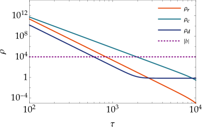
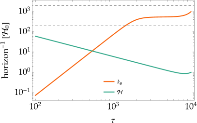
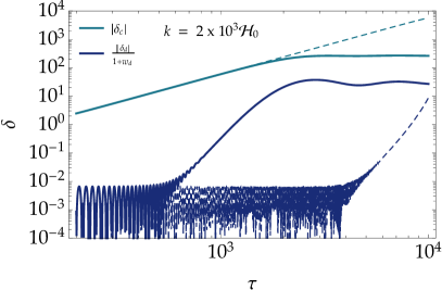
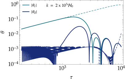
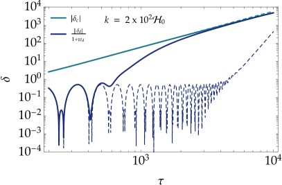
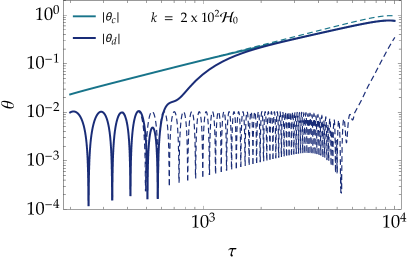
Figure 1: In the upper left panel, we show the evolution of the energy densities $\rho_{r}$, $\rho_{c}$, and $\rho_{d}$ as well as the interaction constant $b=-10^{4}\rho_{0}$ for $r=10^{-6}$. The upper right panel corresponds to the evolution of $k_{s}$ and ${\mathcal{H}}$ normalised by today’s Hubble constant ${\mathcal{H}}_{0}$. We also show two $k$-modes (horizontal dashed-lines) as representatives of a mode that never crossed the DE sound horizon ($k=2\times 10^{3}{\mathcal{H}}_{0}$) and one that was outside the DE sound horizon ($k=2\times 10^{2}{\mathcal{H}}_{0}$) in the strong coupling regime $|b|\gg\rho_{c}$. Since $k_{s}$ is constant in the regime $|b|\gg\rho_{c}$ during the matter era, there is no horizon crossing of the different Fourier modes. In the middle and lower panels, we plot the evolution of the density contrasts and velocity potentials for the modes $k=2\times 10^{3}{\mathcal{H}}_{0}$ and $k=2\times 10^{2}{\mathcal{H}}_{0}$, respectively, with the initial conditions $\delta_{c,{\rm ini}}=1$ and $\delta_{d,{\rm ini}}=\theta_{c,{\rm ini}}=\theta_{d,{\rm ini}}=0$. The evolution for the non-interacting case ($b=0$) is also plotted as dashed lines. The dynamics of perturbations does not depend on the choice of initial conditions because the system is rapidly driven to the attractor solution corresponding to the growing mode of $\delta_{c}$. The different regimes explained in the analytical results of Sec. V can be easily recognized. In particular, we observe the suppressed growth of $\delta_{c}$ for modes inside the effective DE sound horizon ($k>k_{s}$) with respect to the non-interacting case and that the two fluids comove ($\theta_{c}\simeq\theta_{d}$) in the strong coupling regime.

In Fig. 1 the evolution of background and perturbed quantities is plotted for $b=-10^{4}\rho_{0}$ for $r=10^{-6}$, where $\rho_{0}=3H_{0}^{2}/(8\pi G)$ is today’s critical density. In the upper panels, we show the relevant background quantities where we can see how the dark radiation energy density $\rho_{dr}=\rho_{\Lambda}ra^{-4}$ is negligible relative to $\rho_{c}$ and $\rho_{\Lambda}$. We also observe the time at which the strong coupling regime ($|b|>\rho_{c}$) sets in. As we estimated in Eqs. (106) and (107), the inverse of the effective DE horizon scale evolves as $k_{s}\propto\tau^{3}$ in the regime $\rho_{c}/|b|\gg 1$. After entering the strong coupling regime, $k_{s}$ approaches a constant during matter dominance and it starts to increase after the onset of cosmic acceleration. The scale dependence of perturbations arises by the fact that the epoch at which the DE sound horizon crossing occurs (or does not occur) depends on the wavenumber $k$.

In the middle and lower panels of Fig. 1, we show the evolution of the density contrasts and velocity potentials for the modes $k=2\times 10^{3}{\mathcal{H}}_{0}$ and $k=2\times 10^{2}{\mathcal{H}}_{0}$, respectively, where ${\cal H}_{0}$ is today’s Hubble parameter. Although these modes may correspond to the non-linear scales of structure formation, we have chosen for illustrative purposes to understand the behavior of CDM and DE perturbations in the presence of couplings.

For the model parameters under consideration, the mode $k=2\times 10^{3}{\mathcal{H}}_{0}$ has been always inside the DE sound horizon ($k>k_{s}$) by today. As we showed in Eq. (115), the CDM density contrast grows as $\delta_{c}\propto a$ in the weak coupling regime ($\rho_{c}\gg|b|$) of matter era. The DE density contrast first exhibits a rapid oscillation due to the dominance of the homogeneous mode $\delta_{d}^{\rm H}$ over the special solution $\delta_{d}^{\rm slow}$ in Eq. (113). This fast oscillation ceases after $\delta_{d}^{\rm slow}$ dominates over $\delta_{d}^{\rm H}$, whose property can be seen in the middle left panel of Fig. 1. After the perturbations enter the strong coupling regime ($\rho_{c}\ll|b|$), $\delta_{c}$ is nearly frozen as estimated by Eq. (117). This leads to the suppression for the growth of $\delta_{c}$ with respect to the non-interacting case (which is shown as dashed lines). In this regime, we can also confirm the relation (118), i.e., $\delta_{d}/(1+w_{d})\simeq{\rm constant}$ with a suppressed amplitude relative to $\delta_{c}$.

In the middle right panel of Fig. 1, we observe how the two fluids tend to move together, i.e., $\theta_{c}\simeq\theta_{d}$ in the strong coupling regime, which is again in accordance with our analytical estimation given in Eq. (95). This behaviour further illustrates the fact that the suppressed CDM clustering is related to the suppression of peculiar velocities induced by the DE dragging, whose pressure prevents the appearance of large peculiar motions. For the DE sector, it is apparent how the evolution of its perturbations, both the velocity and density, starts differing from the non-interacting evolution when the condition $|b|\simeq(1+w_{d})\rho_{d}$ is met, while the CDM sector is not affected until the onset of the full strong coupling regime characterized by $|b|=\rho_{c}$.

For the mode $k=2\times 10^{2}{\mathcal{H}}_{0}$ plotted in the bottom panels of Fig. 1, the perturbations crossed outside the effective DE sound horizon ($k<k_{s}$) around the same epoch when they entered the strong coupling regime. In the left panel, we can confirm that the DE and CDM density contrasts obey the adiabatic relation (109) for $k<k_{s}$. In this case the interacting term on the right hand-side of Eq. (102) is negligible, so the evolution of $\delta_{c}$ is similar to that in the uncoupled case. Since the asymptotic value of $w_{d}$ is $-1$, $\delta_{d}$ tends to be smaller than $\delta_{c}$ at late times due to the adiabatic relation $\delta_{d}=(1+w_{d})\delta_{c}$. We note that, even though the growth of $\delta_{c}$ is not suppressed for $k<k_{s}$, the CDM and DE velocities approach a same value in the strong-coupling regime (see the right panel). This fact is in agreement with the analytic estimation given in Sec. V.1.

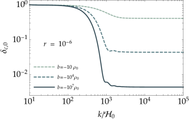
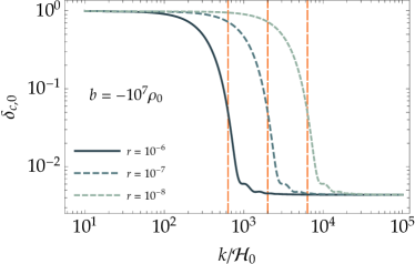
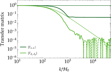
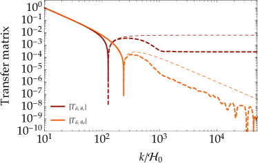
Figure 2: In the upper panels, we plot today’s value of CDM density contrast $\delta_{c,0}$ versus $k/{\mathcal{H}}_{0}$. As explained in the main text, this gives a good approximation to the transfer function for $\delta_{c}$. The left panel shows the dependence with respect to $b$ for $r=10^{-6}$, while the right panel shows how it varies with $r$ for $b=-10^{7}\rho_{0}$. We can see how the parameter $r$ mainly determines the values of $k_{s}$ (shown by the vertical lines in the right panel) around which there is a suppression of $\delta_{c}$ and the parameter $b$ fixes the suppression. In these figures, we notice some small oscillations that are reminiscent of acoustic oscillations produced by dark radiation in the DE component as the modes cross the effective DE sound horizon. In the lower panels, we present all the relevant elements of the transfer matrix for $\delta_{c}$ with $b=-10^{4}\rho_{0}$ and $r=10^{-6}$ involving density contrasts (lower left) and velocity potentials (lower right). We show in solid (dashed) lines the positive (negative) values of each matrix element. For comparison, we plot the non-interacting case in thinner lines to illustrate how the suppression affects all the transfer matrix components. These figures show how the diagonal term clearly dominates over the off-diagonal components, as claimed in the main text, which justifies neglecting them in the computation of the effect for the CDM density contrast.

In the upper left panel of Fig. 2, we plot the CDM density contrast evaluated today (denoted as $\delta_{c,0}$) as a function of $k/{\mathcal{H}}_{0}$ for $r=10^{-6}$ with three different values of $b$. Again, we present the results comprising the non-linear clustering regimes ($k\gtrsim 500{\mathcal{H}}_{0}$) for illustrative purposes. As we discussed in Sec. V.2, the growth of $\delta_{c}$ is suppressed in the strong coupling regime for small-scale modes inside the effective DE sound horizon. For increasing $|b|$, the perturbations enter the strong coupling regime earlier, so the modes with suppressed growth of $\delta_{c}$ span in the region with smaller values of $k$. From Eq. (120), the amplitude of CDM density contrast has the dependence $\delta_{c}/\delta_{c}^{b=0}\propto|b|^{-1/3}$, whose property can be confirmed in Fig. 2.

In the upper right panel of Fig. 2, we show $\delta_{c,0}$ versus $k/{\mathcal{H}}_{0}$ for $b=-10^{7}\rho_{0}$ with three different values of $r$. Since $k_{s}$ has the dependence (121), the smaller $r$ leads to a shift of the region with suppressed values of $\delta_{c}$ toward larger $k$. This means that we need to go to large values of $r$ to include larger scales in the suppression band. Since this parameter has an upper bound imposed by the maximum fraction of dark radiation in the early Universe, there should be an upper limit for the largest scale that can undergo a clustering suppression. As already mentioned, we need $r\lesssim 10^{-6}$ for the initial fraction of dark radiation to be smaller than 1 % in comparison to standard radiation. In the strong coupling regime of matter dominance, we showed that $k_{s}$ is constant, see Eq. (107). On using the approximations $ra^{-4}\ll 1$ and $\rho_{d}\simeq\rho_{\Lambda}$ in this period, the effective DE sound speed is given by $c_{\rm eff}\simeq(2/3)\sqrt{\Omega_{\Lambda}/\Omega_{c}}\sqrt{r}\,a^{-1/2}$. Since ${\cal H}\simeq H_{0}\sqrt{\Omega_{c}}\,a^{-1/2}$ during the matter domination, it follows that

$$k_{s}\simeq\frac{3}{2}\frac{{\mathcal{H}}_{0}}{\sqrt{r}}\frac{\Omega_{c}}{\sqrt{\Omega_{\Lambda}}}\,.$$ (123)

For $\Omega_{c}\simeq 0.3$ and $\Omega_{\Lambda}\simeq 0.7$, the upper bound $r\lesssim 10^{-6}$ translates to the lower bound on $k_{s}$ with the minimum value $k_{s,{\rm min}}\sim 500{\mathcal{H}}_{0}$. As we observe in the upper right panel of Fig. 2, the transition of $\delta_{c,0}$ with respect to $k$ is not very sharp, so there are scales larger than this bound (say, $100{\mathcal{H}}_{0}\lesssim k\lesssim 500{\mathcal{H}}_{0}$) where the CDM density contrast is subject to suppression.

Let us also discuss the off-diagonal terms for the transfer matrix of perturbations expressed as a vector form $\vec{X}=(\delta_{c},\delta_{d},\theta_{c},\theta_{d})$. Denoting $\vec{X}_{\rm ini}$ and $\vec{X}_{0}$ as the initial and present values of $\vec{X}$, respectively, the transfer matrix $\hat{T}$ relates them according to $\vec{X}_{0}=\hat{T}\vec{X}_{\rm ini}$. In particular, for the CDM density contrast, we have

$$\delta_{c,0}=T_{\delta_{c}\delta_{c}}\delta_{c,\rm ini}+T_{\delta_{c}\delta_{d}}\delta_{d,\rm ini}+T_{\delta_{c}\theta_{c}}\theta_{c,\rm ini}+T_{\delta_{c}\theta_{d}}\theta_{d,\rm ini}\,.$$ (124)

Numerically, the components of the transfer matrix relevant to $\delta_{c}$ can be computed by evaluating $\delta_{c}$ at the final time with initial conditions given by the vectors of the canonical basis, i.e., with $\vec{X}_{\rm ini}=(1,0,0,0)$, $\vec{X}_{\rm ini}=(0,1,0,0)$, $\vec{X}_{\rm ini}=(0,0,1,0)$, $\vec{X}_{\rm ini}=(0,0,0,1)$, respectively. We have computed all the relevant components of the transfer matrix in Fig. 2, where we observe that the diagonal component $T_{\delta_{c}\delta_{c}}$ is clearly the dominant one over the others. This together with the fact that the CDM perturbations have a larger amplitude at the onset of the interacting regime, justifies the initial conditions we have chosen to study the suppressed clustering.

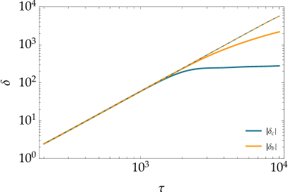
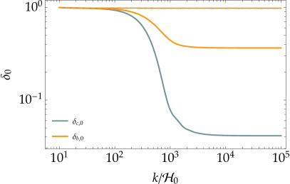
Figure 3: In this figure, we illustrate the effect of CDM and DE momentum exchange on the baryon density contrast $\delta_{b}$ for $b=-10^{4}\rho_{0}$ and $r=10^{-6}$. The left panel shows the evolution of $\delta_{c}$ and $\delta_{b}$ for a Fourier mode $k=2\times 10^{3}{\mathcal{H}}_{0}$ (which is inside the effective DE sound horizon). Unlike $\delta_{c}$, we see how $\delta_{b}$ is subject to a much milder suppression as compared to the non-interacting case (thinner lines). This property is also confirmed in the right panel, where today’s values of $\delta_{b}$ and $\delta_{c}$ versus $k/{\mathcal{H}}_{0}$ are shown. This milder suppression arises because the effect on the baryon perturbation is only indirect due to the less clustering of CDM that induces a smaller gravitational potential so baryons fall into shallower wells and, therefore, they cluster less. On the other hand, the CDM is affected by the pressure of the DE component that prevents the clustering in a more direct and efficient manner.

Finally, we also solved the perturbation equations of baryons and found that, unlike $\delta_{c}$, the growth of $\delta_{b}$ is more mildly suppressed in the regime $\rho_{c}\ll|b|$ (see Fig. 3). The underlying reason is that, while CDM is directly affected by the interaction so that the DE pressure prevents the clustering, the baryons only feel the effect of the reduced clustering of CDM through the smaller gravitational potential that gives rise to a weaker clustering as compared to the non-interacting case.

VII Conclusions

In this work, we have explored a scenario where the dark sector of the Universe contains CDM and DE described by perfect fluids with the Schutz-Sorkin action that interact via a velocity-dependent coupling. The interaction is characterized by the function $f(Z)$, where $Z=g_{\mu\nu}u_{c}^{\mu}u_{c}^{\nu}$ is the scalar product of four velocities.

In many phenomenological approaches taken in the literature, the interactions in the dark sector are added by hand at the background level. A drawback of introducing the interactions at the background level is that the study of the perturbations (which is of paramount importance for testing the theoretical and phenomenological viability of the models) requires a covariantization of the interaction and this process inevitably comes in with ambiguities. Our scenario naturally avoids this problem because the background and perturbation equations of motion unambiguously follow from an explicit action of perfect fluids with a momentum exchange. We also note that the interacting theory of Ref. Asghari et al. (2019), that also avoids ambiguities by starting with a covariant formulation, is different from ours in that the former introduced a velocity-dependent coupling at the level of the continuity equations.

Due to the nature of the interaction, the only modification to the background equations appears as a constant term $f(Z)$ with $Z=-1$. Since this term can be absorbed into a cosmological constant, the momentum exchange does not modify the dynamical evolution of the background cosmology. However, the interaction affects the perturbation equations of the CDM and DE velocity potentials through the momentum exchange. We have derived the linear perturbation equations of motion without fixing gauges and obtained the conditions for the absence of ghosts and Laplacian instabilities. These stability conditions can be easily guaranteed by imposing the usual weak/null energy conditions and a negative coupling constant $b$ in the dark sector. The fact that the interaction only affects the Euler equations has important implications from phenomenological and observational viewpoints. Firstly, the background is oblivious to the interaction and, consequently, the homogeneous evolution cannot constrain the corresponding coupling parameter. Secondly, the perturbed continuity equation remains the same as in $\Lambda$CDM so the relation between the density field and the divergence of the velocity field still holds even though the evolution of both is modified.

After developing the general formalism of dealing with cosmological perturbations in our interacting theory, we proposed a concrete model in which the DE sector contains a cosmological constant and dark radiation. In this model the DE fluid behaves as dark radiation with the equation of state $w_{d}\simeq 1/3$ at early times, so this allows a possibility for alleviating the $H_{0}$ tension present in the $\Lambda$CDM model. After the perturbations enter the strong coupling regime characterized by $|b|>\rho_{c}$, the peculiar velocity of CDM approaches that of DE, i.e., $\theta_{c}\simeq\theta_{d}$. For the wavenumber $k$ in the range $k>k_{s}$, where $k_{s}={\cal H}/c_{\rm eff}$ is the inverse of an effective DE sound horizon associated with the propagation speed squared (104), we have analytically shown that the CDM density contrast $\delta_{c}$ approaches a constant in the strong coupling regime of matter dominance. This results in the suppression for the growth of $\delta_{c}$ in comparison to the uncoupled case ($b=0$). For the modes $k<k_{s}$, the density contrasts in the region $|b|>\rho_{c}$ evolve adiabatically ($\delta_{d}\simeq(1+w_{d})\delta_{c}$), without the suppressed growth of $\delta_{c}$. We have corroborated our analytical findings by numerically solving the perturbation equations and found perfect agreement.

The suppression of the CDM density contrast found in this work is in line with previous findings in the literature supporting the idea that the momentum exchange in the dark sector can alleviate the $\sigma_{8}$ tension. Moreover, in our concrete interacting model, there exists dark radiation in the early Universe that may ease the $H_{0}$ tension. These properties encourage further investigations on their cosmological viability. For the scenario considered in this work, it would be desirable to perform a detailed fit to cosmological data to confirm its ability to resolve said tensions. Work is in progress in this direction.

Appendix A Equations in synchronous gauge

In this Appendix, we give the perturbation equations in the synchronous gauge defined by the perturbed line element

$${\rm d}s^{2}=a^{2}(\tau)\left[-{\rm d}\tau^{2}+(\delta_{ij}+h_{ij}){\rm d}x^{i}{\rm d}x^{j}\right]\,,$$ (125)

where the perturbed spatial metric components are written in terms of the scalar perturbations $h$ and $\eta$ as $h_{ij}={\rm diag}(-2\eta,-2\eta,h+\eta)$. In this gauge, the continuity and Euler equations for CDM and DE perturbations are given by

$$\left(\delta_{c}^{\rm sync}\right)^{\prime} = -\left(\theta_{c}^{\rm sync}+\frac{1}{2}h^{\prime}\right)\,,$$ (126)

$$\left(\theta_{c}^{\rm sync}\right)^{\prime} = -\mathcal{H}\theta_{c}^{\rm sync}+b\frac{3{\cal H}(1+w_{d})\rho_{d}[\theta_{c}^{\rm sync}-(1+c_{d}^{2})\theta_{d}^{\rm sync}]-k^{2}c_{d}^{2}\rho_{d}\delta_{d}^{\rm sync}}{(1+w_{d})\rho_{d}(\rho_{c}-b)-b\rho_{c}}\,,$$ (127)

$$\left(\delta_{d}^{\rm sync}\right)^{\prime} = -3\mathcal{H}(c_{d}^{2}-w_{d})\delta_{d}^{\rm sync}-(1+w_{d})\left(\theta_{d}^{\rm sync}+\frac{1}{2}h^{\prime}\right)\,,$$ (128)

$$\left(\theta_{d}^{\rm sync}\right)^{\prime} = (-1+3c_{d}^{2})\mathcal{H}\theta_{d}^{\rm sync}+\frac{\rho_{c}[k^{2}c_{d}^{2}\rho_{d}\delta_{d}^{\rm sync}+3{\cal H}b\{(1+c_{d}^{2})\theta_{d}^{\rm sync}-\theta_{c}^{\rm sync}\}]-k^{2}bc_{d}^{2}\rho_{d}\delta_{d}^{\rm sync}}{(1+w_{d})\rho_{d}(\rho_{c}-b)-b\rho_{c}}\,.$$ (129)

The suppression of the CDM density contrast explained in detail in the Newtonian gauge also occurs in the same manner as in the synchronous gauge, since the density contrast for modes deep inside the horizon is gauge-invariant to a good approximation.

References

- Spergel et al. (2003) D. Spergel et al. (WMAP), Astrophys. J. Suppl. 148, 175 (2003), arXiv:astro-ph/0302209 .
- Ade et al. (2014) P. Ade et al. (Planck), Astron. Astrophys. 571, A16 (2014), arXiv:1303.5076 [astro-ph.CO] .
- Riess et al. (1998) A. G. Riess et al. (Supernova Search Team), Astron. J. 116, 1009 (1998), arXiv:astro-ph/9805201 .
- Perlmutter et al. (1999) S. Perlmutter et al. (Supernova Cosmology Project), Astrophys. J. 517, 565 (1999), arXiv:astro-ph/9812133 .
- Eisenstein et al. (2005) D. J. Eisenstein et al. (SDSS), Astrophys. J. 633, 560 (2005), arXiv:astro-ph/0501171 .
- Tegmark et al. (2006) M. Tegmark et al. (SDSS), Phys. Rev. D 74, 123507 (2006), arXiv:astro-ph/0608632 .
- Blake et al. (2011) C. Blake et al., Mon. Not. Roy. Astron. Soc. 415, 2876 (2011), arXiv:1104.2948 [astro-ph.CO] .
- Hildebrandt et al. (2017) H. Hildebrandt et al., Mon. Not. Roy. Astron. Soc. 465, 1454 (2017), arXiv:1606.05338 [astro-ph.CO] .
- Abbott et al. (2018) T. Abbott et al. (DES), Phys. Rev. D 98, 043526 (2018), arXiv:1708.01530 [astro-ph.CO] .
- Peebles (1984) P. Peebles, Astrophys. J. 284, 439 (1984).
- Peebles (1982) P. Peebles, Astrophys. J. Lett. 263, L1 (1982).
- Weinberg (1989) S. Weinberg, Rev. Mod. Phys. 61, 1 (1989).
- Martin (2012) J. Martin, Comptes Rendus Physique 13, 566 (2012), arXiv:1205.3365 [astro-ph.CO] .
- Riess et al. (2016) A. G. Riess et al., Astrophys. J. 826, 56 (2016), arXiv:1604.01424 [astro-ph.CO] .
- Aghanim et al. (2020) N. Aghanim et al. (Planck), Astron. Astrophys. 641, A6 (2020), arXiv:1807.06209 [astro-ph.CO] .
- Verde et al. (2019) L. Verde, T. Treu, and A. Riess, Nature Astron. 3, 891 (2019), arXiv:1907.10625 [astro-ph.CO] .
- Riess et al. (2019) A. G. Riess, S. Casertano, W. Yuan, L. M. Macri, and D. Scolnic, Astrophys. J. 876, 85 (2019), arXiv:1903.07603 [astro-ph.CO] .
- Wong et al. (2020) K. C. Wong et al., Mon. Not. Roy. Astron. Soc. 498, 1420 (2020), arXiv:1907.04869 [astro-ph.CO] .
- Reid et al. (2019) M. Reid, D. Pesce, and A. Riess, Astrophys. J. Lett. 886, L27 (2019), arXiv:1908.05625 [astro-ph.GA] .
- Macaulay et al. (2013) E. Macaulay, I. K. Wehus, and H. K. Eriksen, Phys. Rev. Lett. 111, 161301 (2013), arXiv:1303.6583 [astro-ph.CO] .
- Nesseris et al. (2017) S. Nesseris, G. Pantazis, and L. Perivolaropoulos, Phys. Rev. D 96, 023542 (2017), arXiv:1703.10538 [astro-ph.CO] .
- Joudaki et al. (2018) S. Joudaki et al., Mon. Not. Roy. Astron. Soc. 474, 4894 (2018), arXiv:1707.06627 [astro-ph.CO] .
- Karwal and Kamionkowski (2016) T. Karwal and M. Kamionkowski, Phys. Rev. D 94, 103523 (2016), arXiv:1608.01309 [astro-ph.CO] .
- Poulin et al. (2019) V. Poulin, T. L. Smith, T. Karwal, and M. Kamionkowski, Phys. Rev. Lett. 122, 221301 (2019), arXiv:1811.04083 [astro-ph.CO] .
- Agrawal et al. (2019) P. Agrawal, F.-Y. Cyr-Racine, D. Pinner, and L. Randall, (2019), arXiv:1904.01016 [astro-ph.CO] .
- Hill et al. (2020) J. C. Hill, E. McDonough, M. W. Toomey, and S. Alexander, Phys. Rev. D 102, 043507 (2020), arXiv:2003.07355 [astro-ph.CO] .
- Ivanov et al. (2020) M. M. Ivanov, E. McDonough, J. C. Hill, M. Simonović, M. W. Toomey, S. Alexander, and M. Zaldarriaga, Phys. Rev. D 102, 103502 (2020), arXiv:2006.11235 [astro-ph.CO] .
- D’Amico et al. (2020) G. D’Amico, L. Senatore, P. Zhang, and H. Zheng, (2020), arXiv:2006.12420 [astro-ph.CO] .
- Di Valentino et al. (2016) E. Di Valentino, A. Melchiorri, and J. Silk, Phys. Lett. B 761, 242 (2016), arXiv:1606.00634 [astro-ph.CO] .
- Vagnozzi (2020) S. Vagnozzi, Phys. Rev. D 102, 023518 (2020), arXiv:1907.07569 [astro-ph.CO] .
- Horndeski (1974) G. W. Horndeski, Int. J. Theor. Phys. 10, 363 (1974).
- Deffayet et al. (2011) C. Deffayet, X. Gao, D. Steer, and G. Zahariade, Phys. Rev. D 84, 064039 (2011), arXiv:1103.3260 [hep-th] .
- Kobayashi et al. (2011) T. Kobayashi, M. Yamaguchi, and J. Yokoyama, Prog. Theor. Phys. 126, 511 (2011), arXiv:1105.5723 [hep-th] .
- Heisenberg (2014) L. Heisenberg, JCAP 05, 015 (2014), arXiv:1402.7026 [hep-th] .
- Tasinato (2014) G. Tasinato, JHEP 04, 067 (2014), arXiv:1402.6450 [hep-th] .
- Beltran Jimenez and Heisenberg (2016) J. Beltran Jimenez and L. Heisenberg, Phys. Lett. B 757, 405 (2016), arXiv:1602.03410 [hep-th] .
- Tsujikawa (2010) S. Tsujikawa, Lect. Notes Phys. 800, 99 (2010), arXiv:1101.0191 [gr-qc] .
- Peirone et al. (2019) S. Peirone, G. Benevento, N. Frusciante, and S. Tsujikawa, Phys. Rev. D 100, 063540 (2019), arXiv:1905.05166 [astro-ph.CO] .
- De Felice et al. (2016) A. De Felice, L. Heisenberg, R. Kase, S. Mukohyama, S. Tsujikawa, and Y.-l. Zhang, JCAP 06, 048 (2016), arXiv:1603.05806 [gr-qc] .
- De Felice et al. (2017) A. De Felice, L. Heisenberg, and S. Tsujikawa, Phys. Rev. D 95, 123540 (2017), arXiv:1703.09573 [astro-ph.CO] .
- De Felice et al. (2020a) A. De Felice, C.-Q. Geng, M. C. Pookkillath, and L. Yin, JCAP 08, 038 (2020a), arXiv:2002.06782 [astro-ph.CO] .
- Heisenberg and Villarrubia-Rojo (2020) L. Heisenberg and H. Villarrubia-Rojo, (2020), arXiv:2010.00513 [astro-ph.CO] .
- De Felice et al. (2011) A. De Felice, T. Kobayashi, and S. Tsujikawa, Phys. Lett. B 706, 123 (2011), arXiv:1108.4242 [gr-qc] .
- Tsujikawa (2015) S. Tsujikawa, Phys. Rev. D 92, 044029 (2015), arXiv:1505.02459 [astro-ph.CO] .
- Amendola et al. (2018) L. Amendola, M. Kunz, I. D. Saltas, and I. Sawicki, Phys. Rev. Lett. 120, 131101 (2018), arXiv:1711.04825 [astro-ph.CO] .
- Kase and Tsujikawa (2019) R. Kase and S. Tsujikawa, Int. J. Mod. Phys. D 28, 1942005 (2019), arXiv:1809.08735 [gr-qc] .
- Amendola (2004) L. Amendola, Phys. Rev. D 69, 103524 (2004), arXiv:astro-ph/0311175 .
- Tsujikawa (2007) S. Tsujikawa, Phys. Rev. D 76, 023514 (2007), arXiv:0705.1032 [astro-ph] .
- Ade et al. (2016) P. Ade et al. (Planck), Astron. Astrophys. 594, A14 (2016), arXiv:1502.01590 [astro-ph.CO] .
- Pourtsidou et al. (2013) A. Pourtsidou, C. Skordis, and E. Copeland, Phys. Rev. D 88, 083505 (2013), arXiv:1307.0458 [astro-ph.CO] .
- Boehmer et al. (2015) C. G. Boehmer, N. Tamanini, and M. Wright, Phys. Rev. D 91, 123003 (2015), arXiv:1502.04030 [gr-qc] .
- Skordis et al. (2015) C. Skordis, A. Pourtsidou, and E. Copeland, Phys. Rev. D 91, 083537 (2015), arXiv:1502.07297 [astro-ph.CO] .
- Koivisto et al. (2015) T. S. Koivisto, E. N. Saridakis, and N. Tamanini, JCAP 09, 047 (2015), arXiv:1505.07556 [astro-ph.CO] .
- Pourtsidou and Tram (2016) A. Pourtsidou and T. Tram, Phys. Rev. D 94, 043518 (2016), arXiv:1604.04222 [astro-ph.CO] .
- Dutta et al. (2017) J. Dutta, W. Khyllep, and N. Tamanini, Phys. Rev. D 95, 023515 (2017), arXiv:1701.00744 [gr-qc] .
- Linton et al. (2018) M. S. Linton, A. Pourtsidou, R. Crittenden, and R. Maartens, JCAP 04, 043 (2018), arXiv:1711.05196 [astro-ph.CO] .
- Kase and Tsujikawa (2020a) R. Kase and S. Tsujikawa, Phys. Rev. D 101, 063511 (2020a), arXiv:1910.02699 [gr-qc] .
- Kase and Tsujikawa (2020b) R. Kase and S. Tsujikawa, Phys. Lett. B 804, 135400 (2020b), arXiv:1911.02179 [gr-qc] .
- Chamings et al. (2020) F. N. Chamings, A. Avgoustidis, E. J. Copeland, A. M. Green, and A. Pourtsidou, Phys. Rev. D 101, 043531 (2020), arXiv:1912.09858 [astro-ph.CO] .
- Amendola and Tsujikawa (2020) L. Amendola and S. Tsujikawa, JCAP 06, 020 (2020), arXiv:2003.02686 [gr-qc] .
- Kase and Tsujikawa (2020c) R. Kase and S. Tsujikawa, JCAP 11, 032 (2020c), arXiv:2005.13809 [gr-qc] .
- De Felice et al. (2020b) A. De Felice, S. Nakamura, and S. Tsujikawa, Phys. Rev. D 102, 063531 (2020b), arXiv:2004.09384 [gr-qc] .
- Erickson et al. (2002) J. K. Erickson, R. Caldwell, P. J. Steinhardt, C. Armendariz-Picon, and V. F. Mukhanov, Phys. Rev. Lett. 88, 121301 (2002), arXiv:astro-ph/0112438 .
- Bean and Dore (2004) R. Bean and O. Dore, Phys. Rev. D 69, 083503 (2004), arXiv:astro-ph/0307100 .
- Lin et al. (2019) M.-X. Lin, G. Benevento, W. Hu, and M. Raveri, Phys. Rev. D 100, 063542 (2019), arXiv:1905.12618 [astro-ph.CO] .
- Lin et al. (2020) M.-X. Lin, W. Hu, and M. Raveri, Phys. Rev. D 102, 123523 (2020), arXiv:2009.08974 [astro-ph.CO] .
- Asghari et al. (2019) M. Asghari, J. Beltrán Jiménez, S. Khosravi, and D. F. Mota, JCAP 04, 042 (2019), arXiv:1902.05532 [astro-ph.CO] .
- Jiménez et al. (2020) J. B. Jiménez, D. Bettoni, D. Figueruelo, and F. A. Teppa Pannia, JCAP 08, 020 (2020), arXiv:2004.14661 [astro-ph.CO] .
- Schutz and Sorkin (1977) B. F. Schutz and R. Sorkin, Annals Phys. 107, 1 (1977).
- Brown (1993) J. Brown, Class. Quant. Grav. 10, 1579 (1993), arXiv:gr-qc/9304026 .
- De Felice et al. (2010) A. De Felice, J.-M. Gerard, and T. Suyama, Phys. Rev. D 81, 063527 (2010), arXiv:0908.3439 [gr-qc] .
- Dalal et al. (2001) N. Dalal, K. Abazajian, E. E. Jenkins, and A. V. Manohar, Phys. Rev. Lett. 87, 141302 (2001), arXiv:astro-ph/0105317 .
- Chimento et al. (2003) L. P. Chimento, A. S. Jakubi, D. Pavon, and W. Zimdahl, Phys. Rev. D 67, 083513 (2003), arXiv:astro-ph/0303145 .
- Wang et al. (2005) B. Wang, Y.-g. Gong, and E. Abdalla, Phys. Lett. B 624, 141 (2005), arXiv:hep-th/0506069 .
- Wei and Zhang (2007) H. Wei and S. N. Zhang, Phys. Lett. B 644, 7 (2007), arXiv:astro-ph/0609597 .
- Amendola et al. (2007) L. Amendola, G. Camargo Campos, and R. Rosenfeld, Phys. Rev. D 75, 083506 (2007), arXiv:astro-ph/0610806 .
- Guo et al. (2007) Z.-K. Guo, N. Ohta, and S. Tsujikawa, Phys. Rev. D 76, 023508 (2007), arXiv:astro-ph/0702015 .
- Valiviita et al. (2008) J. Valiviita, E. Majerotto, and R. Maartens, JCAP 07, 020 (2008), arXiv:0804.0232 [astro-ph] .
- Salvatelli et al. (2014) V. Salvatelli, N. Said, M. Bruni, A. Melchiorri, and D. Wands, Phys. Rev. Lett. 113, 181301 (2014), arXiv:1406.7297 [astro-ph.CO] .
- Kumar and Nunes (2016) S. Kumar and R. C. Nunes, Phys. Rev. D 94, 123511 (2016), arXiv:1608.02454 [astro-ph.CO] .
- Di Valentino et al. (2017) E. Di Valentino, A. Melchiorri, and O. Mena, Phys. Rev. D 96, 043503 (2017), arXiv:1704.08342 [astro-ph.CO] .
- Yang et al. (2018) W. Yang, S. Pan, E. Di Valentino, R. C. Nunes, S. Vagnozzi, and D. F. Mota, JCAP 09, 019 (2018), arXiv:1805.08252 [astro-ph.CO] .
- Pan et al. (2019) S. Pan, W. Yang, E. Di Valentino, E. N. Saridakis, and S. Chakraborty, Phys. Rev. D 100, 103520 (2019), arXiv:1907.07540 [astro-ph.CO] .
- Di Valentino et al. (2020) E. Di Valentino, A. Melchiorri, O. Mena, and S. Vagnozzi, Phys. Rev. D 101, 063502 (2020), arXiv:1910.09853 [astro-ph.CO] .
- Maroto (2006) A. L. Maroto, JCAP 0605, 015 (2006), arXiv:astro-ph/0512464 [astro-ph] .
- Beltran Jimenez and Maroto (2007) J. Beltran Jimenez and A. L. Maroto, Phys. Rev. D76, 023003 (2007), arXiv:astro-ph/0703483 [astro-ph] .
- Beltran Jimenez and Maroto (2009) J. Beltran Jimenez and A. L. Maroto, JCAP 0903, 015 (2009), arXiv:0811.3606 [astro-ph] .
- Harko and Lobo (2013) T. Harko and F. S. N. Lobo, JCAP 1307, 036 (2013), arXiv:1304.0757 [gr-qc] .
- Cembranos et al. (2019) J. Cembranos, A. Maroto, and H. Villarrubia-Rojo, JCAP 06, 041 (2019), arXiv:1903.11009 [astro-ph.CO] .
- García-García et al. (2016) C. García-García, A. L. Maroto, and P. Martín-Moruno, JCAP 12, 022 (2016), arXiv:1608.06493 [gr-qc] .
- Ballesteros et al. (2014) G. Ballesteros, B. Bellazzini, and L. Mercolli, JCAP 05, 007 (2014), arXiv:1312.2957 [hep-th] .
- Simpson (2010) F. Simpson, Phys. Rev. D 82, 083505 (2010), arXiv:1007.1034 [astro-ph.CO] .
- Bardeen (1980) J. M. Bardeen, Phys. Rev. D 22, 1882 (1980).
- Buen-Abad et al. (2015) M. A. Buen-Abad, G. Marques-Tavares, and M. Schmaltz, Phys. Rev. D 92, 023531 (2015), arXiv:1505.03542 [hep-ph] .
- Lesgourgues et al. (2016) J. Lesgourgues, G. Marques-Tavares, and M. Schmaltz, JCAP 02, 037 (2016), arXiv:1507.04351 [astro-ph.CO] .
- Buen-Abad et al. (2018) M. A. Buen-Abad, M. Schmaltz, J. Lesgourgues, and T. Brinckmann, JCAP 01, 008 (2018), arXiv:1708.09406 [astro-ph.CO] .
- Raveri et al. (2017) M. Raveri, W. Hu, T. Hoffman, and L.-T. Wang, Phys. Rev. D 96, 103501 (2017), arXiv:1709.04877 [astro-ph.CO] .
- Blinov and Marques-Tavares (2020) N. Blinov and G. Marques-Tavares, JCAP 09, 029 (2020), arXiv:2003.08387 [astro-ph.CO] .