Tropical compactification via Ganter’s algorithm

Abstract.

We describe a canonical compactification of a polyhedral complex in Euclidean space. When the recession cones of the polyhedral complex form a fan, the compactified polyhedral complex is a subspace of a tropical toric variety. In this case, the procedure is analogous to the tropical compactifications of subvarieties of tori.

We give an analysis of the combinatorial structure of the compactification and show that its Hasse diagram can be computed via Ganter’s algorithm. Our algorithm is implemented in and shipped with polymake.

1. Introduction

Most of the first steps in tropical geometry considered the tropicalisation of subvarieties of tori [RST05]. Yet early on Mikhalkin considered the compactification of tropical curves and amoebas in toric surfaces [Mik04], and then of hypersurfaces in toric varieties [Mik04a]. Later Payne described “extended tropicalisations” for subvarieties of toric varieties [Pay09]. These extended tropicalisations apply the tropicalisation of subvarieties of tori in an orbit by orbit fashion. Previous to this, Tevelev used tropicalisations to define well-behaved compactifications of classical algebraic subvarieties in the torus [Tev07]. In this setup, the tropicalisation of a subvariety of the torus determines a toric variety suitable for the compactification of the original variety.

Our main goal here is to analyse combinatorially and computationally the structure of canonical compactifications of tropical varieties. More concretely, given a tropical variety in Euclidean space, we describe a canonical compactification of the underlying polyhedral complex which is compatible with the compactifications of single polyhedra described in [Rab12]. To define the canonical compactification of a tropical variety, all geometric data needed is encoded in a choice of polyhedral structure on the original tropical variety.

Throughout we let $N$ be a lattice and $N_{{\mathbb{R}}}=N\otimes_{\mathbb{Z}}{\mathbb{R}}$. Given a polyhedron ${P}=\{x\in N_{{\mathbb{R}}}|Ax\geq b\}$, its recession cone is $\operatorname{{rec}}({P})=\{x\in N_{{\mathbb{R}}}|\ Ax\geq 0\}$.

Definition .

Let ${\mathcal{P}\mathcal{C}}$ be a polyhedral complex in $N_{{\mathbb{R}}}$. We say that ${\mathcal{P}\mathcal{C}}$ has a recession fan if for any ${P},Q\in{\mathcal{P}\mathcal{C}}$ the intersection $\operatorname{{rec}}({P})\cap\operatorname{{rec}}(Q)$ is a face of both $\operatorname{{rec}}({P})$ and $\operatorname{{rec}}(Q)$. In that case the recession cones of the polyhedra in ${\mathcal{P}\mathcal{C}}$ form a fan, and we call this fan the recession fan of ${\mathcal{P}\mathcal{C}}$, denoted by $\operatorname{{rec}}({\mathcal{P}\mathcal{C}})$.

A polyhedral complex may or may not have a recession fan [BS11]. In the case when it does, we prove the following theorem.

Theorem (subsection 3.2).

If a polyhedral complex ${\mathcal{P}\mathcal{C}}$ has a recession fan, then its canonical compactification ${\overline{{\mathcal{P}\mathcal{C}}}}$ is a polyhedral complex in the tropical toric variety of the fan $\operatorname{{rec}}({\mathcal{P}\mathcal{C}})$.

By [OR13, Remark 3.13] any polyhedral complex ${\mathcal{P}\mathcal{C}}$ has a compactifying fan which can be obtained by choosing a fan that is a refinement of the set of cones $\cup_{{P}\in{\mathcal{P}\mathcal{C}}}\operatorname{{rec}}({P})$. In fact, if we consider a polyhedral complex ${\mathcal{P}\mathcal{C}}$ and an arbitrary fan $\Delta$, many of our algorithmic results are still applicable if $\Delta$ refines all the cones $\operatorname{{rec}}({P})$ for ${P}\in{\mathcal{P}\mathcal{C}}$, see Definition 2.1. However, even if $\operatorname{{rec}}({\mathcal{P}\mathcal{C}})$ is not a fan we can nonetheless define a canonical compactification of ${\mathcal{P}\mathcal{C}}$ without taking any refinements, as long as the recession cone of each face is pointed. However, the resulting compactification is not a polyhedral complex in a tropical toric variety. It is a more general abstract polyhedral space in the sense of [JRS18, Definition 2.1] or subsection 2.1.

Theorem (subsection 3.2).

The canonical compactification ${\overline{{\mathcal{P}\mathcal{C}}}}$ is an abstract polyhedral space.

Here we will describe the compactification ${\overline{{\mathcal{P}\mathcal{C}}}}$ via the Hasse diagram of its face lattice. A Hasse diagram is a graphical representation of a partially ordered set. The vertices, also known as nodes, of the Hasse diagram correspond to elements of the set and the edges correspond to covering relations, with edges being directed upwards, towards the larger sets. One very efficient algorithm for computing Hasse diagrams or general closure systems is Ganter’s algorithm [Gan10]. To use Ganter’s algorithm we have to construct a closure operator for our setting. This closure operator takes any subset of vertices to the smallest face containing it. Therefore, applying Ganter’s algorithm first necessitates the expression of the vertices and faces of the compactification in the data encoding the original polyhedral complex.

Our algorithmic results give rise to a closure operator in section 4. For the concrete problem of determining ${\overline{{\mathcal{P}\mathcal{C}}}}$ it turns out that no new geometric information is needed, hence we can state the following theorem.

Theorem .

The Hasse diagram of the compactification ${\overline{{\mathcal{P}\mathcal{C}}}}$ can be computed via Ganter’s algorithm in a purely combinatorial way.

Our implementation is shipped with the combinatorial software framework polymake [GJ00] since release 3.6, and hence it is available via many package managers on Linux and in the MacOS polymake bundle. It can even be used on Windows via the Windows Subsystem for Linux (WSL). Furthermore, polymake is interfaced in Julia [Bez+17] via Polymake.jl [KLT20]. Hence our algorithm is accessible to a large community of mathematicians, namely the users of polymake and Julia, and it is embedded in frameworks that provide a wide variety of tools for analysing and using the tropical compactification. By using polymake we took advantage of its existing templated version of Ganter’s algorithm by Simon Hampe and Ewgenij Gawrilow. The necessary data types, like Hasse diagrams, polyhedral complexes, tropical varieties, and chain complexes are already implemented in polymake, making our codebase slim and easy to maintain. For using the compactification in subsequent research, polymake already has cellular sheaves [KSW17] and patchworkings [JV20], as well as many other tools from tropical geometry. Last, but not least, polymake comes with a built in serialization framework, such that the compactification can easily be stored in a file, and testing framework, ensuring robustness of our implementation.

In fact, our main motivation to study canonical compactifications is to extend the use of the polymake extension cellularSheaves for tropical homology and patchwork to compact tropical varieties. In the case of tropicalisations of projective complex varieties satisfying additional assumptions, the dimensions of the tropical homology groups are equal to the corresponding Hodge numbers. The assumption that the variety is projective implicitly assumes that the tropicalisation under consideration is an extended tropicalisation in the sense of Payne or Mikhalkin, and is hence compact. Therefore, the Hasse diagram of the compactification is necessary for such computations, together with a signed incidence relation that we describe in section 5.

In section 2 we will give the necessary definitions from tropical and algorithmic geometry for our setup. Afterwards in section 3 we describe the Hasse diagram of the compactification for both a single polyhedron and a polyhedral complex. The data structure of the compactification is described in section 4. In section 5, we give a simple algorithm for computing a signed incidence relation necessary for computing cohomology of cellular sheaves. Lastly, section 6 contains examples with code computed in polymake. Throughout the text we emphasis many examples which exhibit the pathologies of the canonical compactification, as well as its many applications to tropical geometry and beyond.

1.1. Acknowledgements

We are very grateful to Michael Joswig for advice throughout the implementation and for suggesting the connection to Ganter’s algorithm. We are very grateful to Benjamin Lorenz for advice on designing our codebase and for helping to solve many complex implementation specific issues.

We also thank Joswig, Marta Panizzut, and Paul Vater for their comments which helped us improve a preliminary draft of this paper.

2. Preliminaries

2.1. Tropical toric varieties and polyhedral complexes

In this section we will describe the basic setup, following the definitions and notation of [OR13], [Pay09], [MR]. Throughout we let $N\cong\mathbb{Z}^{n}$ denote a lattice and $N_{{\mathbb{R}}}=N\otimes_{\mathbb{Z}}{\mathbb{R}}$.

Definition .

[OR13, 2.4] For a rational polyhedral fan $\Delta\subseteq N_{{\mathbb{R}}}$ the tropical toric variety ${N_{{\mathbb{R}}}}(\Delta)$ of $N_{{\mathbb{R}}}$ with respect to $\Delta$ is

$${N_{{\mathbb{R}}}}(\Delta)\ :=\ \mathop{{\coprod}}_{\sigma\in\Delta}N_{{\mathbb{R}}}/\operatorname{{span}}(\sigma).$$

The tropical toric variety ${N_{{\mathbb{R}}}}(\Delta)$ is equipped with the unique topology such that

• The inclusions $N_{{\mathbb{R}}}/\operatorname{{span}}(\sigma)\hookrightarrow{N_{{\mathbb{R}}}}(\Delta)$ are continuous for any cone $\sigma\in\Delta$.

• For any $x\in N_{{\mathbb{R}}}$ and any $v\in N_{{\mathbb{R}}}$, the sequence $\left(x+nv\right)_{n\in\mathbb{N}}\in N_{{\mathbb{R}}}$ converges in ${N_{{\mathbb{R}}}}(\Delta)$ if and only if $v$ is contained in the support of the fan $\Delta$.

The reader is directed to [Pay09, Section 3] for more details. The tropical toric variety ${N_{{\mathbb{R}}}}(\Delta)$ is compact if and only if the polyhedral fan $\Delta$ is complete. We denote the single stratum $N_{{\mathbb{R}}}/\operatorname{{span}}(\sigma)$ by ${N_{{\mathbb{R}}}}(\sigma)$. If $\Delta$ is a pointed fan, then $N_{{\mathbb{R}}}$ can be canonically identified with the open subset ${N_{{\mathbb{R}}}}({0})\subset{N_{{\mathbb{R}}}}(\Delta)$.

Definition .

A polyhedral complex ${\mathcal{P}\mathcal{C}}$ in a tropical toric variety ${N_{{\mathbb{R}}}}(\Delta)$ is a finite collection of polyhedra in ${N_{{\mathbb{R}}}}(\Delta)$ such that ${\mathcal{P}\mathcal{C}}\cap{N_{{\mathbb{R}}}}(\rho)$ is a polyhedral complex in ${N_{{\mathbb{R}}}}(\rho)\cong\mathbb{R}^{\text{codim}\rho}$ for every cone $\rho$ of $\Delta$, and which satisfies:

1. for a polyhedron ${P}\in{\mathcal{P}\mathcal{C}}$, if $Q$ is a face of ${P}$, which is denoted $Q\leq{P}$, we have $Q\in{\mathcal{P}\mathcal{C}}$;

2. for ${P},{P}^{\prime}\in{\mathcal{P}\mathcal{C}}$, if $Q={P}\cap{P}^{\prime}$ is non-empty then $Q$ is a face of both ${P}$ and ${P}^{\prime}$.

Definition .

[OR13, Definition 3.1] Let $\mathcal{{P}}$ be a finite collection of polyhedra in $N_{{\mathbb{R}}}$, and $\Delta$ a pointed fan. The fan $\Delta$ is said to be compatible with $\mathcal{{P}}$ if for all ${P}\in\mathcal{{P}}$ and all cones $\sigma\in\Delta$, either $\sigma\subset\operatorname{{rec}}({P})$ or $\operatorname{{relint}}(\sigma)\cap\operatorname{{rec}}({P})=\emptyset$.

The fan $\Delta$ is said to be a compactifying fan for $\mathcal{{P}}$ if for all ${P}\in\mathcal{{P}}$, the recession cone is the union of cones in $\Delta$.

Example .

For an example of $\Delta$ being incompatible with ${P}$ consider the following polyhedra:

$$\begin{array}[]{ccc}{P}=\leavevmode\hbox to74.78pt{\vbox to46.12pt{\text{[drawing]}}}&\mbox{ and }&\Delta=\leavevmode\hbox to46.12pt{\vbox to46.12pt{\text{[drawing]}}}\end{array}.$$

In this case, ${P}=\operatorname{{rec}}({P})$. The fan $\Delta$ has only one maximal cone which intersects $\operatorname{{rec}}({P})$ improperly. This example serves for us to show what goes wrong when ${P}$ and $\Delta$ are incompatible.

Given a polyhedron ${P}\subset N_{{\mathbb{R}}}$ we can take its closure ${\overline{{P}}}$ in ${N_{{\mathbb{R}}}}(\Delta)$. Following [OR13], whether or not ${\overline{{P}}}$ intersects a stratum of ${N_{{\mathbb{R}}}}(\Delta)$ corresponding to a cone $\sigma$ of $\Delta$ depends on the recession cone of ${P}$.

To explicitly describe the intersection of ${\overline{{P}}}$ with each stratum of ${N_{{\mathbb{R}}}}(\Delta)$ we must consider the projections $\pi_{\sigma}:N_{{\mathbb{R}}}{\twoheadrightarrow}{N_{{\mathbb{R}}}}(\sigma)$ for every $\sigma\in\Delta$. Then when the intersection ${\overline{{P}}}\cap{N_{{\mathbb{R}}}}(\sigma)$ is non-empty, it is equal to $\pi_{\sigma}({P})$. These statements are summarised in the following lemma from [OR13].

Lemma ([OR13, Lemma 3.9]).

Let $\Delta$ be a compactifying fan of ${P}$. The compactification ${\overline{{P}}}$ of a polyhedron ${P}$ in ${N_{{\mathbb{R}}}}(\Delta)$ is

$${\overline{{P}}}\ :=\ \mathop{{\coprod}}_{\sigma\in\Delta,\ \operatorname{{relint}}(\sigma)\cap\operatorname{{rec}}({P})\not=\emptyset}\pi_{\sigma}({P}).$$

The main condition to ensure that ${\overline{{P}}}$ is indeed compact is that $\Delta$ is a compactifying fan for ${P}$, meaning that it refines the recession cone of ${P}$. In other words, we have

(1) $$\operatorname{{rec}}({P})\ =\ \bigcup_{\sigma\in\Delta,\ \operatorname{{relint}}(\sigma)\cap\operatorname{{rec}}({P})\not=\emptyset}\sigma.$$

Then ${\overline{{P}}}\cap{N_{{\mathbb{R}}}}(\sigma)\neq\emptyset$ if and only if $\operatorname{{rec}}({P})\cap\operatorname{{relint}}(\sigma)\neq\emptyset$.

Remark .

[OR13, Corollary 3.7] The intersection of the compactification with a stratum ${\overline{{P}}}\cap{N_{{\mathbb{R}}}}(\sigma)$ is the polyhedron $\pi_{\sigma}({P})$ whenever the intersection is non-empty. Notice that the intersection of ${\overline{{P}}}$ with a stratum ${N_{{\mathbb{R}}}}(\sigma)$ is not necessarily compact. That is no surprise, since the intersection with the stratum ${N_{{\mathbb{R}}}}(0)$ is the (non-compact) polyhedron ${P}$ that we started with.

Example ([Rab12, Example 3.20]).

Consider the following ${P}$ having the positive orthant as recession cone:

The compactification has five vertices indicated by dots. For the compactification we chose $\Delta=\operatorname{{rec}}({P})$, the fan having the recession cone of ${P}$ as single maximal cone.

From now on we assume that $\Delta$ has no lineality to avoid effects like in the following example.

Example .

Let ${P}={\mathbb{R}}$, then $\Delta=\operatorname{{rec}}({P})={\mathbb{R}}$, and it is not a pointed fan. Then ${N_{{\mathbb{R}}}}(\Delta)={\overline{{P}}}=\pi_{{\mathbb{R}}}({\mathbb{R}})$ which is just a point. Since $0$ is not a cone of $\Delta$ the set $N_{{\mathbb{R}}}$ cannot even be seen as an open subset of ${N_{{\mathbb{R}}}}(\Delta)$.

Lastly, we give the definition of abstract polyhedral space from [JSS19] and [JRS18]. This describes the structure of the compactification when the recession cones of a polyhedral complex do not form a fan. Here $\mathbb{T}:=[-\infty,\infty)$ and is equipped with the topology of the half open interval. Notice that $\mathbb{T}^{r}=N_{{\mathbb{R}}}(\Delta)$, where $\Delta$ is the cone in ${\mathbb{R}}^{r}$ generated by the $r$ standard basis vectors. Hence it is a tropical toric variety.

Definition .

A polyhedral space $X$ is a paracompact, second countable Hausdorff topological space with an atlas of charts $(\varphi_{\alpha}\colon U_{\alpha}\rightarrow\Omega_{\alpha}\subset X_{\alpha})_{{\alpha}\in A}$ such that:

1. The $U_{\alpha}$ are open subsets of $X$, the $\Omega_{\alpha}$ are open subsets of polyhedral subspaces $X_{\alpha}\subset\mathbb{T}^{r_{\alpha}}$, and the maps $\varphi_{\alpha}\colon U_{\alpha}\rightarrow\Omega_{\alpha}$ are homeomorphisms for all $\alpha$;

2. for all $\alpha,\beta\in A$ the transition maps

   $$\varphi_{\alpha}\circ\varphi^{-1}_{\beta}\colon\varphi_{\beta}(U_{\alpha}\cap U_{\beta})\rightarrow{\varphi_{\alpha}(U_{\alpha}\cap U_{\beta})}$$

   are extended affine linear maps, see [JSS19, Definition 2.18].

2.2. Ganter’s algorithm

We want to use Ganter’s algorithm for computing closure systems in order to compute the Hasse diagram $\operatorname{{HD}}({\overline{{\mathcal{P}\mathcal{C}}}})$ of the compactification ${\overline{{\mathcal{P}\mathcal{C}}}}$. We will follow the notation of [HJS19], the original work by Ganter can be found in [Gan10], which is an English reprint of a German preprint from 1984. The input for Ganter’s algorithm is a closure system.

Definition ([HJS19, Def. 2.1]).

A closure operator on a set $S$ is a function $\operatorname{\mathop{{cl}}}:\mathcal{{\mathcal{P}\mathcal{S}}}(S)\to\mathcal{{\mathcal{P}\mathcal{S}}}(S)$ on the power set of $S$, which fulfills the following axioms for all subsets $A,B\subseteq S$:

1. $A\subseteq\operatorname{\mathop{{cl}}}(A)$ (Extensiveness).

2. If $A\subseteq B$ then $\operatorname{\mathop{{cl}}}(A)\subseteq\operatorname{\mathop{{cl}}}(B)$ (Monotonicity).

3. $\operatorname{\mathop{{cl}}}(\operatorname{\mathop{{cl}}}(A))=\operatorname{\mathop{{cl}}}(A)$ (Idempotency).

A subset $A$ of $S$ is called closed, if $\operatorname{\mathop{{cl}}}(A)=A$. The set of all closed sets of $S$ with respect to some closure operator is called a closure system.

Example .

For a polytope ${P}$, the set $S$ would be the vertices $\operatorname{{vert}}({P})$ and the closure operator $\operatorname{\mathop{{cl}}}(A)$ for $A\subseteq S$ would list the vertices of the smallest face containing $A$. This is also the approach we want to use in our setting.

This use of the closure operator also works for other combinatorial objects, like cones, fans, polyhedral complexes, and flats of matroids, see subsection 3.2.

The idea of Ganter’s algorithm is to start out with the empty set and then successively add vertices until the full closure system is computed. The algorithm is designed in a way that it is output sensitive, i.e. its running time is linear in the number of edges of the Hasse diagram $\operatorname{{HD}}({\overline{{\mathcal{P}\mathcal{C}}}})$.

We will first solve the below steps for the case of our polyhedral complex consisting of a single polyhedron. Afterwards we argue why this extends seamlessly to polyhedral complexes whose recession cones form a fan.

1. Determine what the vertices $\operatorname{{vert}}({\overline{{\mathcal{P}\mathcal{C}}}})$ should be.

2. State an algorithm determining whether a subset of $\operatorname{{vert}}({\overline{{\mathcal{P}\mathcal{C}}}})$ forms a face.

3. Describe the closure operator on $\operatorname{{vert}}({\overline{{\mathcal{P}\mathcal{C}}}})$ algorithmically.

The first two tasks are mainly about rephrasing existing mathematical concepts on ${\overline{{\mathcal{P}\mathcal{C}}}}$ in combinatorial, and later in algorithmic terms. The third task could also be solved in a brute force manner as soon as the second task is done. In particular, for any subset of $\operatorname{{vert}}({\overline{{\mathcal{P}\mathcal{C}}}})$ it must be checked whether or not the subset forms a face. However, we would like to find a solution avoiding the brute force approach, as many of our examples are large and computationally expensive.

3. Hasse diagram of the compactification

3.1. Faces of the compactification of a single polyhedron

In this section we will describe the faces of the compactification ${\overline{{P}}}$ of a polyhedron ${P}$ with respect to its recession cone $\operatorname{{rec}}({P})$. A node in $\operatorname{{HD}}({\overline{{P}}})$ corresponds to a face of ${\overline{{P}}}$, so we have to explain what these faces are. Looking at subsection 2.1, we see that ${\overline{{P}}}$ is made of polyhedra $\pi_{\sigma}({P})$ in the strata $N_{{\mathbb{R}}}(\sigma)$. Notice that the set $\pi_{\sigma}({P})$ is closed in the stratum $N_{{\mathbb{R}}}(\sigma)$, yet it is not closed in ${N_{{\mathbb{R}}}}(\Delta)$.

For two cones $\tau\leq\sigma\in\Delta=\operatorname{{rec}}({P})$ we get a map

$$\pi_{\sigma,\tau}:\ {N_{{\mathbb{R}}}}(\tau){\twoheadrightarrow}{N_{{\mathbb{R}}}}(\sigma),$$

such that $\pi_{\sigma}=\pi_{\sigma,\tau}\circ\pi_{\tau}$. Using this definition, we can describe the compactification ${\overline{F}}$ in ${N_{{\mathbb{R}}}}(\Delta)$ of a face $F\leq\pi_{\tau}({P})$ to be

$${\overline{F}}\ :=\ \mathop{{\coprod}}_{\sigma\in\Delta,\ \tau\leq\sigma,\ \operatorname{{relint}}(\pi_{\tau}(\sigma))\cap\operatorname{{rec}}(F)\not=\emptyset}\pi_{\sigma,\tau}(F).$$

In particular, if $F$ is a compact face of $\pi_{\tau}({P})$, then ${\overline{F}}=F$.

Definition (Face of ${\overline{{P}}}$).

The faces of ${\overline{{P}}}$ are the compactifications ${\overline{F}}$ of any face $F\leq\pi_{\tau}({P})$ of any $\pi_{\tau}({P})$. For a face ${\overline{F}}$ of ${\overline{{P}}}$ that is the compactification of $F\leq\pi_{\tau}({P})$ we call the cone $\operatorname{{trunk}}({\overline{F}}):=\tau$ the trunk of ${\overline{F}}$. The set

$$\operatorname{{support}}({\overline{F}})\ :=\ \{\sigma\in\Delta\ |\ \tau\leq\sigma,\operatorname{{relint}}(\pi_{\tau}(\sigma))\cap\operatorname{{rec}}(F)\not=\emptyset\}$$

are the supporting cones of ${\overline{F}}$.

Note that the trunk is the unique minimal element of $\operatorname{{support}}({\overline{F}})$ and for $F$ being compact, it is the only element of $\operatorname{{support}}({\overline{F}})$.

Example .

In subsection 2.1, note that the face

$$F\ =\ (1,0)+{\mathbb{R}}_{\geq 0}\cdot(1,0)\ =\ \leavevmode\hbox to28.97pt{\vbox to29.73pt{\text{[drawing]}}}$$

of ${P}=\pi_{0}({P})$ is not a face of ${\overline{{P}}}$. However, its compactification, consisting of $F$ and the vertex $\pi_{{\mathbb{R}}_{\geq 0}\times\{0\}}(F)$, is a face of ${\overline{{P}}}$.

Thus we can abbreviate the above formula for ${\overline{F}}$ as

$${\overline{F}}\ :=\ \mathop{{\coprod}}_{\sigma\in\operatorname{{support}}({\overline{F}})}\pi_{\sigma,\tau}(F),$$

where $\tau=\operatorname{{trunk}}({\overline{F}})$. In the following we will abbreviate this even further by denoting the components $\pi_{\sigma,\tau}(F)$ as $F_{\sigma}$.

Remark .

Since we are working in the case $\Delta=\operatorname{{rec}}({P})$, we can reformulate the support condition. From $F\leq\pi_{\tau}({P})$, it follows that $\operatorname{{rec}}(F)\leq\operatorname{{rec}}(\pi_{\tau}({P}))$ and by $\tau\leq\operatorname{{rec}}({P})$, we deduce $\operatorname{{rec}}(\pi_{\tau}({P}))=\pi_{\tau}(\operatorname{{rec}}({P}))$. Clearly, for $\tau\leq\sigma\leq\operatorname{{rec}}({P})$ also $\pi_{\tau}(\sigma)\leq\pi_{\tau}(\operatorname{{rec}}({P}))$. Thence we have two faces of $\pi_{\tau}(\operatorname{{rec}}({P}))$ where the relative interior of the first one intersects the second non-trivially. This means that the first forms a face of the second. So

$$\operatorname{{support}}({\overline{F}})\ =\{\sigma\leq\operatorname{{rec}}({P})\ |\ \tau\leq\sigma,\pi_{\tau}(\sigma)\leq\operatorname{{rec}}(F)\}.$$

Example .

If ${P}$ and $\Delta$ are incompatible, subsection 3.1 becomes invalid.

Consider subsection 2.1, and pick the face $F:=(0,0)$ of ${P}$. Since $F$ is compact itself, we have ${\overline{F}}=F$. But if we project along $\sigma:=\{0\}\times{\mathbb{R}}_{\geq 0}\leq\Delta$, the projection of ${P}$ is the whole ${\mathbb{R}}$ and the projection of $(0,0)$ cannot be a face, since ${\mathbb{R}}$ has no zero-dimensional faces.

Example .

Let us compute the $\operatorname{{support}}$ and $\operatorname{{trunk}}$ for some faces of the compactified polyhedron in subsection 2.1. Note that we will always write the trunk as the first element in the support.

The face ${\overline{F}}$ from subsection 2.1 has $\operatorname{{trunk}}({\overline{F}})=0$ and

$$\operatorname{{support}}({\overline{F}})\ =\ \operatorname{{support}}\left(\leavevmode\hbox to30.17pt{\vbox to28.97pt{\text{[drawing]}}}\right)\ =\ \{0,\ {\mathbb{R}}_{\geq 0}\times\{0\}\}\ =\ \left\{\leavevmode\hbox to23.16pt{\vbox to23.16pt{\text{[drawing]}}},\leavevmode\hbox to23.96pt{\vbox to23.16pt{\text{[drawing]}}}\right\}.$$

Take ${\overline{F^{\prime}}}=F^{\prime}=\pi_{{\mathbb{R}}_{\geq 0}^{2}}({P})$ in the previous example, then

$$\operatorname{{support}}({\overline{F^{\prime}}})\ =\ \operatorname{{support}}\left(\leavevmode\hbox to30.17pt{\vbox to30.17pt{\text{[drawing]}}}\right)\ =\ \{{\mathbb{R}}_{\geq 0}^{2}\}\ =\ \left\{\leavevmode\hbox to23.96pt{\vbox to23.96pt{\text{[drawing]}}}\right\}.$$

And for ${\overline{F^{\prime\prime}}}$ with $F^{\prime\prime}=\pi_{{\mathbb{R}}_{\geq 0}\times\{0\}}({P})$, we get

$$\operatorname{{support}}({\overline{F^{\prime\prime}}})\ =\ \operatorname{{support}}\left(\leavevmode\hbox to30.17pt{\vbox to30.17pt{\text{[drawing]}}}\right)\ =\ \{{\mathbb{R}}_{\geq 0}\times\{0\},\ {\mathbb{R}}_{\geq 0}^{2}\}\ =\ \left\{\leavevmode\hbox to23.96pt{\vbox to23.16pt{\text{[drawing]}}},\leavevmode\hbox to23.96pt{\vbox to23.96pt{\text{[drawing]}}}\right\}.$$

The following lemma will be crucial to show that faces in the sense of subsection 3.1 behave as we expect from faces. In particular, we will need it to guarantee that the faces of ${\overline{{P}}}$ form a polyhedral complex in the sense of subsection 2.1.

Lemma .

Let $F\leq\pi_{\tau}({P})$ be a face and let $\sigma\in\operatorname{{support}}({\overline{F}})$. Then $\pi_{\sigma,\tau}(F)$ is a face of $\pi_{\sigma}({P})$.

Proof.

Since $\pi_{\sigma}=\pi_{\sigma,\tau}\circ\pi_{\tau}$, we may assume that $\tau=0$ without loss of generality. Hence $\pi_{\tau}({P})={P}$.

Let $F\leq{P}$ be a face and let $\sigma\in\operatorname{{support}}({\overline{F}})$. Thus, by subsection 3.1 the cone $\sigma\leq\operatorname{{rec}}(F)$. Since $F\leq{P}$ there is a hyperplane $h\in\operatorname{{Hom}}(N_{{\mathbb{R}}},{\mathbb{R}})$ such that

$$F\ =\ \{p\in{P}\ |\ h(p)\mbox{ is minimal}\}.$$

The hyperplane $h$ evaluates to a constant on $F$, hence the observation $\sigma\leq\operatorname{{rec}}(F)$ implies $h(s)=0$ for all $s\in\sigma$. Thus, the hyperplane $h$ is well-defined on ${N_{{\mathbb{R}}}}(\sigma)$. This means that the set

$$F^{\prime}\ :=\ \{p\in\pi_{\sigma}({P})\ |\ h(p)\mbox{ is minimal}\}$$

is a face of $\pi_{\sigma}({P})$. The observation $F^{\prime}=\pi_{\sigma}(F)$ finishes the proof. ∎

Example .

In subsection 2.1, the projection $\pi_{{\mathbb{R}}_{\geq 0}\times\{0\}}(F)$ is a vertex of $\pi_{{\mathbb{R}}_{\geq 0}\times\{0\}}({P})$. On the other hand, the projection $\pi_{\{0\}\times{\mathbb{R}}_{\geq 0}}(F)$ is not a face of $\pi_{\{0\}\times{\mathbb{R}}_{\geq 0}}({P})$. In this case the support condition of the lemma is violated, and $\{0\}\times{\mathbb{R}}_{\geq 0}$ is not in the support of ${\overline{F}}$.

We will now use subsection 3.1 to show that faces in the sense of subsection 3.1 form a polyhedral complex. We will start by showing that it is compatible with taking faces.

Lemma .

The face relation is transitive, i.e. if ${\overline{F^{\prime}}}\leq{\overline{F}}\leq{\overline{{P}}}$, then ${\overline{F^{\prime}}}\leq{\overline{{P}}}$.

Proof.

By definition ${\overline{F}}\leq{\overline{{P}}}$ means that there exist $\tau\leq\operatorname{{rec}}({P})$ and $F\leq\pi_{\tau}({P})\subset{N_{{\mathbb{R}}}}(\tau)\cong{\mathbb{R}}^{\text{codim}(\tau)}$. When now considering ${\overline{F^{\prime}}}\leq{\overline{F}}$ we want to see $F$ as a polyhedron in $N^{\prime}_{{\mathbb{R}}}:={N_{{\mathbb{R}}}}(\tau)\cong{\mathbb{R}}^{\text{codim}(\tau)}$ and compactify with respect to the recession cone $\operatorname{{rec}}(F)$.

Remember that

$$\operatorname{{support}}({\overline{F}})=\{\sigma\leq\operatorname{{rec}}({P})\ |\ \tau\leq\sigma,\ \pi_{\tau}(\sigma)\leq\operatorname{{rec}}(F)\}.$$

The set $\{\pi_{\tau}(\sigma)\ |\ \sigma\in\operatorname{{support}}({\overline{F}})\}$ forms a fan, it is the fan given by $\operatorname{{rec}}(F)$ and all its faces, hence the fan with respect to which we compactify $F$.

We have the face ${\overline{F^{\prime}}}\leq{\overline{F}}$, thus by definition $F^{\prime}\leq\pi^{\prime}_{\tau^{\prime}}(F)$, where $\pi^{\prime}_{\tau^{\prime}}:N^{\prime}_{{\mathbb{R}}}\to{N_{{\mathbb{R}}}}^{\prime}(\tau^{\prime})$. With the previous considerations $\tau^{\prime}=\pi_{\tau}(\sigma^{\prime})$ for some $\sigma^{\prime}\in\operatorname{{support}}({\overline{F}})$, and then $\pi^{\prime}_{\tau^{\prime}}=\pi_{\sigma^{\prime},\tau}$. So $F^{\prime}\leq\pi_{\sigma^{\prime},\tau}(F)$ and by subsection 3.1 $\pi_{\sigma^{\prime},\tau}(F)\leq\pi_{\sigma^{\prime}}({P})$. Thus $F^{\prime}$ also gives a face ${\overline{F^{\prime}}}$ of ${\overline{{P}}}$. We can see that the support of ${\overline{F^{\prime}}}$ in ${\overline{F}}$ is the support of ${\overline{F^{\prime}}}$ in ${\overline{{P}}}$ mapped with $\pi_{\tau}$, also the components of the compactification agree. Thence, the compactification of $F^{\prime}$ is the same when compactifying it as a face of $\pi^{\prime}_{\tau^{\prime}}(F)$ or as face of $\pi_{\sigma^{\prime}}({P})$. This yields the desired face relation ${\overline{F^{\prime}}}\leq{\overline{{P}}}$. ∎

The following lemma shows that the intersection of two compact faces is again a face in the sense of subsection 3.1.

Lemma .

Let ${\overline{F}},{\overline{F^{\prime}}}\leq{\overline{{P}}}$ be two faces of ${\overline{{P}}}$, then the intersection ${\overline{F}}\cap{\overline{F^{\prime}}}\leq{\overline{{P}}}$ is also a face.

Proof.

We have $F\leq\pi_{\tau}({P})$ and $F^{\prime}\leq\pi_{\tau^{\prime}}({P})$. Let us look at the intersection in a stratum ${N_{{\mathbb{R}}}}(\sigma)$:

$$\begin{array}[]{rl}{\overline{F}}\cap{\overline{F^{\prime}}}\cap{N_{{\mathbb{R}}}}(\sigma)&=({\overline{F}}\cap{N_{{\mathbb{R}}}}(\sigma))\cap({\overline{F^{\prime}}}\cap{N_{{\mathbb{R}}}}(\sigma))\\ &=\begin{cases}\pi_{\sigma,\tau}(F)\cap\pi_{\sigma,\tau^{\prime}}(F^{\prime})&\sigma\in\operatorname{{support}}({\overline{F}})\cap\operatorname{{support}}({\overline{F^{\prime}}})\\ \emptyset&\mbox{ else.}\\ \end{cases}\end{array}$$

By subsection 3.1 we have the face relations $\pi_{\sigma,\tau}(F)\leq\pi_{\sigma}({P})$ and $\pi_{\sigma,\tau^{\prime}}(F^{\prime})\leq\pi_{\sigma}({P})$ and thus the intersection

$$G_{\sigma}:=\pi_{\sigma,\tau}(F)\cap\pi_{\sigma,\tau^{\prime}}(F^{\prime})\leq\pi_{\sigma}({P})$$

is a face of the polyhedron $\pi_{\sigma}({P})$.

Our approach is to show that these $G_{\sigma}$ form the components of a face of ${\overline{{P}}}$. First we construct a candidate for the support, in order to find the $\operatorname{{trunk}}:={{t}}$, from this we show that the $G_{\sigma}$ form the compactification of $G_{{t}}\leq\pi_{{t}}({P})$.

If ${\overline{F}}\cap{\overline{F^{\prime}}}$ is a face, its support should be

$$\begin{array}[]{rl}\operatorname{{support}}({\overline{F}}\cap{\overline{F^{\prime}}})&=\operatorname{{support}}({\overline{F}})\cap\operatorname{{support}}({\overline{F^{\prime}}})\\ &=\left\{\sigma\in\Delta\ \mid\begin{array}[]{l}\tau\leq\sigma,\ \pi_{\tau}(\sigma)\leq\operatorname{{rec}}(F),\\ \tau^{\prime}\leq\sigma,\ \pi_{\tau^{\prime}}(\sigma)\leq\operatorname{{rec}}(F^{\prime})\end{array}\right\}\\ \end{array}$$

If this set is non-empty, it contains a unique minimal element ${{t}}$. Otherwise suppose that $\sigma_{1}\not=\sigma_{2}$ are both minimal elements of the set. Then both contain $\tau$ as a face, thus their intersection $\sigma_{1}\cap\sigma_{2}$ does so, too. Now for the other condition, it holds for $i=1,2$ that $\pi_{\tau}(\sigma_{i})\leq\operatorname{{rec}}(F)$. Hence, the intersection $\pi_{\tau}(\sigma_{1})\cap\pi_{\tau}(\sigma_{2})=\pi_{\tau}(\sigma_{1}\cap\sigma_{2})$ must be a face of $\operatorname{{rec}}(F)$ as well. The same applies to $\tau^{\prime}$. Thus $\sigma_{1}\cap\sigma_{2}$ is an element of the set and strictly included in $\sigma_{i}$, contradicting our assumption.

Now set $G:=G_{{{t}}}\leq\pi_{{{t}}}({P})$. Then by definition ${\overline{G}}\leq{\overline{{P}}}$. It remains to show that ${\overline{G}}={\overline{F}}\cap{\overline{F^{\prime}}}$. The concatenation law $\pi_{\sigma}=\pi_{\sigma,\tau}\circ\pi_{\tau}$ extends to $\pi_{\sigma,{{t}}}\circ\pi_{{{t}},\tau}=\pi_{\sigma,\tau}$ if $\tau$ is a face of ${{t}}$. One uses this to verify the equality ${\overline{G}}={\overline{F}}\cap{\overline{F^{\prime}}}$ on the non-trivial strata, i.e. those of $\operatorname{{support}}({\overline{F}})\cap\operatorname{{support}}({\overline{F^{\prime}}})$. ∎

Remark .

In the proof of subsection 3.1 we use $\Delta=\operatorname{{rec}}({P})$. Otherwise the intersection $\pi_{\tau}(\sigma_{1}\cap\sigma_{2})$ might not be a face of $\operatorname{{rec}}(F)$.

These lemmata ensure that by compactifying with respect to the recession cone, we obtain a polyhedral complex in the sense of subsection 2.1.

Proposition .

The compactification ${\overline{{P}}}$ of a polyhedron ${P}$ inside the tropical toric variety of its recession cone ${N_{{\mathbb{R}}}}(\operatorname{{rec}}({P}))$ is a polyhedral complex in the sense of subsection 2.1.

Proof.

The first point is elaborated in subsection 2.1, the second point is subsection 3.1 and the third subsection 3.1. ∎

Faces ${\overline{F}}$ of the compactification ${\overline{{P}}}$ are closely related to faces of ${P}$, in the following sense:

Lemma .

Let $F\leq\pi_{\sigma}({P})$ be a face. Then the preimage $\pi^{-1}_{\sigma}(F)\cap{P}$ is a face of ${P}$.

Proof.

The face $F\leq\pi_{\sigma}({P})$ is cut out by a hyperplane $h\in\operatorname{{Hom}}({N_{{\mathbb{R}}}}(\sigma),{\mathbb{R}})$, i.e.

$$F\ =\ \{p\in\pi_{\sigma}({P})\ |\ h(p)\mbox{ is minimal}\}.$$

The preimage $\pi^{-1}_{\sigma}(F)\cap{P}$ is cut out by the composition $h\circ\pi_{\sigma}$. ∎

In the following lemma we will show that each face ${\overline{F}}$ of the compactification ${\overline{{P}}}$ is associated to a unique face of ${P}$. A key ingredient is subsection 3.1 which ensures that the stratification is compatible with the face structure.

Lemma .

Let ${\overline{F}}$ be a face of ${\overline{{P}}}$. Let $\tau:=\operatorname{{trunk}}({\overline{F}})$. Then for any $\sigma\in\operatorname{{support}}({\overline{F}})$ we have

$$\pi_{\sigma}^{-1}(F_{\sigma})\cap{P}\ =\ \pi_{\tau}^{-1}(F_{\tau})\cap{P}.$$

We call the face $\pi_{\tau}^{-1}(F_{\tau})\cap{P}$ the parent face of ${\overline{F}}$, and denote this as $\operatorname{{parent}}({\overline{F}})$.

Proof.

Assume for now that $\tau=0$. Then $\pi_{\tau}$ is just the identity and we have to show that

$$F\ =\ (\pi_{\sigma}^{-1}\circ\pi_{\sigma}(F))\cap{P}$$

for any cone $\sigma\in\operatorname{{support}}({\overline{F}})$. Just as in the proof of subsection 3.1, the face $F$ is cut out from ${P}$ by a hyperplane $h\in\operatorname{{Hom}}(N_{{\mathbb{R}}},{\mathbb{R}})$ and because of $\sigma\leq\operatorname{{rec}}(F)$ this hyperplane is well-defined on ${N_{{\mathbb{R}}}}(\sigma)$. Thus, the hyperplane $h$ cuts out $\pi_{\sigma}(F)\leq\pi_{\sigma}({P})$. Both $\pi_{\sigma}$ and $\pi_{\sigma}^{-1}$ preserve the value of $h$, meaning that for any point $p\in{N_{{\mathbb{R}}}}(\sigma)$ we have $h(p)=h(q)$ for all points $q\in\pi_{\sigma}^{-1}(p)$ in the preimage. Denote by $h(F)$ the value of $h$ on $F$. Then

$$(\pi_{\sigma}^{-1}\circ\pi_{\sigma}(F))\cap{P}\ =\ \{p\in{P}\ |\ h(p)=h(F)\}.$$

The above argument also shows that $\pi_{\sigma,\tau}^{-1}(F_{\sigma})\cap\pi_{\tau}({P})=F_{\tau}$. Together with the identity $\pi_{\sigma}=\pi_{\sigma,\tau}\circ\pi_{\tau}$ this finishes the proof. ∎

Remark .

Let ${\overline{F}}\leq{\overline{{P}}}$ with $\operatorname{{trunk}}({\overline{F}})=\tau$. Then the following equality holds

$$F=\pi_{\tau}(\operatorname{{parent}}({\overline{F}})).$$

Example .

In subsection 2.1 the parent face of the vertex $\pi_{{\mathbb{R}}_{\geq 0}\times\{0\}}((1,0)+{\mathbb{R}}_{\geq 0}\cdot(1,0))$ is $(1,0)+{\mathbb{R}}_{\geq 0}\cdot(1,0)$ itself.

Remark .

With the notation of parent face, we can simplify the support condition for ${\overline{F}}$, even further. From the statement in subsection 3.1 to

$$\operatorname{{support}}({\overline{F}})\ =\ \{\sigma\in\operatorname{{rec}}({P})\ |\ \operatorname{{trunk}}({\overline{F}})\leq\sigma\leq\operatorname{{rec}}(\operatorname{{parent}}({\overline{F}}))\}.$$

Face relations between compact faces lift to a face relation of the parent faces.

Lemma .

Let ${\overline{F^{\prime}}}\leq{\overline{F}}$ be two faces of ${\overline{{P}}}$. Then the same face relation holds for the parents, namely

$$\operatorname{{parent}}({\overline{F^{\prime}}})\ \leq\ \operatorname{{parent}}({\overline{F}}).$$

Proof.

As in the proof of subsection 3.1 we have $F\leq\pi_{\tau}({P})$ and $F^{\prime}\leq\pi_{\sigma,\tau}(F)\leq\pi_{\sigma}({P})$ for some $\sigma\in\operatorname{{support}}({\overline{F}})$. Now

$$\operatorname{{parent}}({\overline{F^{\prime}}})=\pi_{\sigma}^{-1}(F^{\prime})\cap{P}\leq{P}$$

and

$$\operatorname{{parent}}({\overline{F}})=\pi_{\tau}^{-1}(F)\cap{P}=\pi_{\sigma}^{-1}(F_{\sigma})\cap{P}\leq{P}.$$

Since $F^{\prime}\subset F_{\sigma}$, also $\operatorname{{parent}}({\overline{F^{\prime}}})\subset\operatorname{{parent}}({\overline{F}})$ and because both are faces of ${P}$, we get the required face relation of the parent faces. ∎

Definition .

Every face of ${\overline{{P}}}$ with trunk $\sigma$ canonically inherits the dimension of the underlying face of the $\pi_{\sigma}({P})$, i.e. for $F\leq\pi_{\sigma}({P})$ we set

$$\dim({\overline{F}})\ =\ \dim(F).$$

Topologically subsection 3.1 makes sense. The dimension of ${\overline{F}}$ should be the maximal length of a chain of faces of ${\overline{F}}$.

Let ${\overline{F^{0}}}<{\overline{F^{1}}}<\dots<{\overline{F^{d}}}={\overline{F}}$ be a chain of faces of maximal length. Then we can consider the parent faces of the ${\overline{F^{i}}}$. By subsection 3.1 this gives a chain of faces of $\operatorname{{parent}}({\overline{F}})$. This also works when only taking the “partial parent” $\pi^{-1}_{\sigma,\tau}(F^{i}_{\sigma})\cap F$, and gives a chain of faces of $F$. On the other hand, the compactifications of a chain of faces of $F$ gives a chain of faces of ${\overline{F}}$.

After equipping faces of ${\overline{{P}}}$ with a dimension, it makes sense to talk about vertices, i.e. faces of dimension zero.

Proposition .

The vertices of ${\overline{{P}}}$ are the union of all the vertices of the $\pi_{\sigma}({P})$.

Proof.

The main point is that all the vertices of the $\pi_{\sigma}({P})$ are already compact. Since compactification preserves dimension, there cannot be more vertices. ∎

Proposition .

The vertices of ${\overline{{P}}}$ are in one-to-one correspondence with faces $F$ of ${P}$ such that $\dim{F}=\dim{\operatorname{{rec}}(F})$.

Proof.

First assume we have $F\leq{P}$ with $\dim{F}=\dim{\operatorname{{rec}}(F)}$. Now we choose $\sigma=\operatorname{{rec}}(F)$. Then the projection $\pi_{\sigma}(F)$ is just a point. By subsection 3.1 it is a face of $\pi_{\sigma}({P})$.

Conversely, assume we are given a vertex $v$ of ${\overline{{P}}}$. By subsection 3.1 we know it is the vertex of some $\pi_{\sigma}({P})$. subsection 3.1 gives that $F:=\operatorname{{parent}}(v)$ is a face of ${P}$. From subsection 3.1 we obtain $\pi_{\sigma}(F)=v$. Since $\dim(v)=0$, it has to hold that $\dim(F)=\dim(\operatorname{{rec}}(F))$. ∎

Remark .

As in the previous proof and using subsection 3.1 and subsection 3.1, we can rewrite subsection 3.1 to

$$\dim({\overline{F}})=\dim(F)=\dim(\operatorname{{parent}}({\overline{F}}))-\dim(\operatorname{{trunk}}({\overline{F}})).$$

Example .

In subsection 3.1 consider the face ${\mathbb{R}}_{\geq 0}\cdot(-1,1)$ of ${P}$. This does not give rise to a vertex.

If $\operatorname{{rec}}({P})$ is only refined by $\Delta$ as in Equation 1 of subsection 2.1, one face with $\dim{F}=\dim{\operatorname{{rec}}(F)}$ can give rise to multiple vertices of ${\overline{{P}}}$ depending on how many $\sigma\in\Delta$ there are with $\dim(\sigma)=\dim(\operatorname{{rec}}(F))$ and $\sigma\subseteq\operatorname{{rec}}(F)$.

Take for example the following $\Delta$ in subsection 2.1:

$$\begin{array}[]{cc}\Delta&{P}\mbox{ and }{\overline{{P}}}\\[8.5359pt] \leavevmode\hbox to72.3pt{\vbox to72.3pt{\text{[drawing]}}}&\leavevmode\hbox to87.24pt{\vbox to87.24pt{\text{[drawing]}}}\end{array}$$

In this case the compactification has four new vertices instead of three.

One could refine the polyhedral complex, i.e. replace the polyhedron by a polyhedral complex ${\mathcal{P}\mathcal{C}}$ such that $\Delta=\operatorname{{rec}}({\mathcal{P}\mathcal{C}})$ and $\operatorname{{support}}({\mathcal{P}\mathcal{C}})={P}$. But in this case the compactification would end up having five vertices. Hence, refinement does not serve as a trick to apply our implementation for $\Delta\not=\operatorname{{rec}}({\mathcal{P}\mathcal{C}})$.

3.2. Compatibility of the single compactifications for polyhedral complexes

In this section we prove that the compactification ${\overline{{\mathcal{P}\mathcal{C}}}}$ is an abstract polyhedral space. In the particular case when the polyhedral complex ${\mathcal{P}\mathcal{C}}$ has a recession fan, we show that ${\overline{{\mathcal{P}\mathcal{C}}}}$ forms a polyhedral complex in the tropical toric variety ${N_{{\mathbb{R}}}}(\operatorname{{rec}}({\mathcal{P}\mathcal{C}}))$.

For the applications we have in mind, it suffices to consider polyhedral complexes whose recession cones form a fan $\Delta=\operatorname{{rec}}({\mathcal{P}\mathcal{C}})$. In the sense of subsection 2.1, $\Delta$ will automatically be compatible and compactifying for ${\mathcal{P}\mathcal{C}}$. Nevertheless, we give an example for a polyhedral complex ${\mathcal{P}\mathcal{C}}$ that has no recession fan.

Example .

Take the following polyhedral complex in ${\mathbb{R}}^{3}$:

$$\begin{array}[]{ccc}P_{0}&:=&(0,0,1)+{\mathbb{R}}_{\geq 0}\cdot(1,1,0)\\ P_{1}&:=&\operatorname{{conv}}\{(0,0,0),(0,0,1)\}\\ P_{2}&:=&(0,0,0)+{\mathbb{R}}_{\geq 0}\cdot(1,0,0)+{\mathbb{R}}_{\geq 0}\cdot(0,1,0)\end{array}.$$

Here $\operatorname{{rec}}(P_{0})\cap\operatorname{{rec}}(P_{2})=\operatorname{{rec}}(P_{0})$, but $\operatorname{{rec}}(P_{0})$ is not a face of $\operatorname{{rec}}(P_{2})$, hence this polyhedral complex does not have a recession fan.

By [OR13, Remark 3.13] any polyhedral complex ${\mathcal{P}\mathcal{C}}$ has a compactifying fan which can be obtained by choosing a fan that is a refinement of the set of cones $\cup_{{P}\in{\mathcal{P}\mathcal{C}}}\operatorname{{rec}}({P})$.

Example .

Any bounded polyhedral complex has a recession fan, consisting just of the origin. Nevertheless, since these are already compact, they are not interesting for our procedures. Another trivial example for polyhedral complexes that always have a recession fan, are those that consist of one polyhedron and all its faces.

First we inspect the first condition for the compactification to form a polyhedral complex. The following lemma extends [OR13, Corollary 3.7] for a polyhedron to polyhedral complexes.

Lemma .

If ${\mathcal{P}\mathcal{C}}$ has a recession fan $\Delta$, then the intersection of the compactification of ${\mathcal{P}\mathcal{C}}$ with respect to $\Delta$ with a stratum ${\overline{{\mathcal{P}\mathcal{C}}}}\cap{N_{{\mathbb{R}}}}(\rho)$ forms a polyhedral complex in ${\mathbb{R}}^{\text{codim}{\rho}}$.

Proof.

The intersection with the stratum ${N_{{\mathbb{R}}}}(\rho)$ consists of the following polyhedra

$$\begin{array}[]{rl}{\overline{{\mathcal{P}\mathcal{C}}}}\cap{N_{{\mathbb{R}}}}(\rho)&=\{{\overline{{P}}}\cap{N_{{\mathbb{R}}}}(\rho)\ |\ {P}\in{\mathcal{P}\mathcal{C}}\}\\ &=\{\pi_{\rho}({P})\ |\ {P}\in{\mathcal{P}\mathcal{C}},\rho\in\operatorname{{support}}({\overline{{P}}})\}\end{array}.$$

A cone $\rho$ is contained in $\operatorname{{support}}({\overline{{P}}})$ if and only if $\operatorname{{relint}}(\rho)\cap\operatorname{{rec}}({P})\not=\emptyset$. Since $\Delta=\operatorname{{rec}}({\mathcal{P}\mathcal{C}})$ is the recession fan and $\rho,\operatorname{{rec}}({P})\in\Delta$ this condition is equivalent to $\rho\leq\operatorname{{rec}}({P})$, thus

$$\begin{array}[]{rl}{\overline{{\mathcal{P}\mathcal{C}}}}\cap{N_{{\mathbb{R}}}}(\rho)&=\{\pi_{\rho}({P})\ |\ {P}\in{\mathcal{P}\mathcal{C}},\rho\leq\operatorname{{rec}}({P})\}.\\ \end{array}$$

First we show that the first axiom for being a polyhedral complex holds for this collection of polyhedra, namely that if $F\leq\pi_{\rho}({P})$, then $F$ comes from an element of ${\mathcal{P}\mathcal{C}}$. This element is $\operatorname{{parent}}({\overline{F}})$, which is a member of ${\mathcal{P}\mathcal{C}}$ by subsection 3.1, and with subsection 3.1 $F=\pi_{\rho}(\operatorname{{parent}}({\overline{F}}))$.

For the second axiom of a polyhedral complex, let $\pi_{\rho}({P}),\pi_{\rho}({P}^{\prime})\in{\overline{{\mathcal{P}\mathcal{C}}}}\cap{N_{{\mathbb{R}}}}(\rho)$. We want to show that the intersection $\pi_{\rho}({P})\cap\pi_{\rho}({P}^{\prime})\in{\overline{{\mathcal{P}\mathcal{C}}}}\cap{N_{{\mathbb{R}}}}(\rho)$. But $\pi_{\rho}({P})\cap\pi_{\rho}({P}^{\prime})=\pi_{\rho}({P}\cap{P}^{\prime})$. Since ${\mathcal{P}\mathcal{C}}$ is a polyhedral complex ${P}\cap{P}^{\prime}\in{\mathcal{P}\mathcal{C}}$ and by $\rho\leq\operatorname{{rec}}({P}),\operatorname{{rec}}({P}^{\prime})$, also $\rho\leq\operatorname{{rec}}({P}\cap{P}^{\prime})$. Thence, the intersection $\pi_{\rho}({P})\cap\pi_{\rho}({P}^{\prime})\in{\overline{{\mathcal{P}\mathcal{C}}}}\cap{N_{{\mathbb{R}}}}(\rho)$. ∎

In contrast to [OR13, Lemma 3.10/Proposition 3.12], which analyses the support of ${\overline{{\mathcal{P}\mathcal{C}}}}$ in ${N_{{\mathbb{R}}}}(\Delta)$, the following theorem captures the combinatorial structure of a polyhedral complex on ${\overline{{\mathcal{P}\mathcal{C}}}}$.

Theorem .

If ${\mathcal{P}\mathcal{C}}$ has a recession fan $\Delta$, then the compactification ${\overline{{\mathcal{P}\mathcal{C}}}}$ in ${N_{{\mathbb{R}}}}(\Delta)$ forms a polyhedral complex.

Proof.

For ${\overline{{\mathcal{P}\mathcal{C}}}}$ to form a polyhedral complex, we have to check the three points from subsection 2.1.

1. This is subsection 3.2.

2. The proof of subsection 3.1 can be used here. The fact that we glue does not affect this condition.

3. Let $Q={\overline{F}}\leq{\overline{{P}}}$ and $Q^{\prime}={\overline{F^{\prime}}}\leq{\overline{{P}^{\prime}}}$. If ${P}={P}^{\prime}$, then $Q\cap Q^{\prime}\in{\overline{{P}}}\subset{\overline{{\mathcal{P}\mathcal{C}}}}$ by subsection 3.1. Let us investigate the case ${P}\neq{P}^{\prime}$. Without loss of generality $F=\pi_{\tau}({P})$ and $F^{\prime}=\pi_{\tau^{\prime}}({P}^{\prime})$. (Just choose ${P}=\operatorname{{parent}}({\overline{F}})$.) And

   $$\operatorname{{support}}({\overline{F}})=\operatorname{{support}}({\overline{\pi_{\tau}({P})}})=\{\sigma\in\operatorname{{rec}}({\mathcal{P}\mathcal{C}})\ |\ \tau\leq\sigma\leq\operatorname{{rec}}({P})\}.$$

   Thence,

   $$\begin{array}[]{rl}\operatorname{{support}}({\overline{F}})\cap\operatorname{{support}}({\overline{F^{\prime}}})&=\left\{\sigma\in\operatorname{{rec}}({\mathcal{P}\mathcal{C}})\ |\ \begin{array}[]{l}\tau\leq\sigma\leq\operatorname{{rec}}({P})\\ \tau^{\prime}\leq\sigma\leq\operatorname{{rec}}({P}^{\prime})\\ \end{array}\right\}\\ &=\left\{\sigma\in\operatorname{{rec}}({\mathcal{P}\mathcal{C}})\ |\ \langle\tau+\tau^{\prime}\rangle\leq\sigma\leq\operatorname{{rec}}({P}\cap{P}^{\prime})\right\}\end{array}$$

   As already elaborated in the proof of subsection 3.1 this set has a minimal element $t$.

   The intersection of ${\overline{F}}\cap{\overline{F^{\prime}}}$ with a stratum ${N_{{\mathbb{R}}}}(\sigma)$ for $\sigma\in\operatorname{{support}}({\overline{F}})\cap\operatorname{{support}}({\overline{F^{\prime}}})$ is

   $$\begin{array}[]{rl}{\overline{F}}\cap{\overline{F^{\prime}}}\cap{N_{{\mathbb{R}}}}(\sigma)&=\pi_{\sigma,\tau}(F)\cap\pi_{\sigma,\tau^{\prime}}(F)\\ &=\pi_{\sigma}({P})\cap\pi_{\sigma}({P}^{\prime})\\ &=\pi_{\sigma}({P}\cap{P}^{\prime})\end{array},$$

   otherwise it is empty. Then ${\overline{F}}\cap{\overline{F^{\prime}}}={\overline{\pi_{t}({P}\cap{P}^{\prime})}}$. This is a face of ${\overline{{P}\cap{P}^{\prime}}}\leq{\overline{{P}}}$ and by the previous point in ${\overline{{\mathcal{P}\mathcal{C}}}}$. It is also a face of ${\overline{{P}^{\prime}}}$. Since we glue along faces, we have exactly one element in ${\overline{{\mathcal{P}\mathcal{C}}}}$.

∎

Example .

A tropical hypersurface $X_{f}$ in $\mathbb{R}^{n}$ is defined by a tropical polynomial $f$ which is a convex piecewise integral affine function. The Newton polytope $NP_{f}$ is the support of the hypersurface $X_{f}$. The hypersurface is also equipped with weights on its top dimensional faces [MS15]. The collection of recession cones of the faces of $X_{f}$ is a fan $\Delta_{f}$. In fact, it is the codimension one skeleton of the dual fan of the Newton polytope of $f$.

The compactification of $X_{f}$ in $N_{\mathbb{R}}(\Delta_{f})$ is a stratified space. The strata are in correspondence with the faces $\{F\}$ of $NP(f)$ and each stratum is a tropical hypersurface coming from the restriction $f|_{F}$ of the tropical polynomial to the monomials corresponding to lattice points contained in $F$.

Example .

If $M$ is a matroid on the ground set $\{0,\dots,n\}$ of rank $d+1$, the matroidal fan $\Sigma(M)$ of $M$ is a simplicial fan in $\mathbb{R}^{n+1}/\langle(1,\dots,1)\rangle$ which is isomorphic to the cone over the order complex of the lattice of flats of $M$ [AK06]. The fan $\Sigma(M)$ also defines a tropical toric variety $TV_{\mathbb{T}}({\Sigma(M)}).$ Compactifying the fan face by face or taking its closure in $TV_{\mathbb{T}}({\Sigma(M)})$ yield the same complex $\overline{\Sigma(M)}$. Since the fan is simplicial, the faces of the compactification are all cubes. In general, if the fan is simplicial, one obtains the so called canonical compactification of [AP20, 1.4]. The tropical homology [Ite+16] of the fan $\overline{\Sigma(M)}$ is isomorphic to the Chow ring of a matroid of [FS05] by [AP20].

There are other simplicial fan structures on the set $\text{Supp}(\Sigma(M))$ coming from building sets [FS05]. Distinct fan structures give distinct compactifications and the tropical homology of these compactifications are also distinct. However for a fan structure coming from a building set $\mathcal{G}$ we have $H^{q}(\Sigma(M,\mathcal{G});\mathcal{F}^{p})=0$ if $p\neq q$ and $A^{2k}(M,\mathcal{G})\cong H^{k}(\Sigma(M,\mathcal{G});\mathcal{F}^{k})$ otherwise.

Tropical linear spaces are polyhedral complexes in Euclidean space coming from valuated matroids [Spe04]. The recession fan of a tropical linear space is supported on the fan of the underlying matroid of the valuated matroid. Therefore, for a suitable fan structure $\Sigma(M)$, the compactification of a tropical linear space is a polyhedral complex in $TV_{\mathbb{T}}({\Sigma(M)})$.

If ${\mathcal{P}\mathcal{C}}$ does not have a recession fan, we can describe a compactification ${\overline{{\mathcal{P}\mathcal{C}}}}$ by compactifying every polyhedron in its recession cone. The resulting object does not live in a tropical toric variety, nevertheless it is a polyhedral space.

Example .

Let ${\mathcal{P}\mathcal{C}}$ be the polyhedral complex from subsection 3.2. It does not have a recession fan, but the following $\Delta$ is a compactifying fan for ${\mathcal{P}\mathcal{C}}$. The fan is given by $\Delta=\{0,\ \rho_{0},\ \rho_{1},\ \rho_{2},\sigma_{1},\ \sigma_{2}\}$ where $\rho_{0}={\mathbb{R}}_{\geq 0}(1,\ 0,\ 0)$, $\rho_{1}={\mathbb{R}}_{\geq 0}(1,\ 1,\ 0)$, $\rho_{2}={\mathbb{R}}_{\geq 0}(0,\ 1,\ 0)$, $\sigma_{1}={\mathbb{R}}_{\geq 0}\rho_{0}+{\mathbb{R}}_{\geq 0}\rho_{1}$ and $\sigma_{2}={\mathbb{R}}_{\geq 0}\rho_{1}+{\mathbb{R}}_{\geq 0}\rho_{2}$.

Then $\operatorname{{support}}({P}_{0})=\{0,\rho_{1}\}$, $\operatorname{{support}}({P}_{1})=\{0\}$ and $\operatorname{{support}}({P}_{2})=\Delta$. For the lower-dimensional faces of ${P}_{i}$ there are only two interesting ones: $\rho_{0}\leq{P}_{2}$ with support $\{0,\rho_{2}\}$ and $\rho_{2}\leq{P}_{2}$ with support $\{0,\rho_{2}\}$.

Consider the intersection with the stratum ${N_{{\mathbb{R}}}}(\rho_{1})$:

$${\overline{{\mathcal{P}\mathcal{C}}}}\cap{N_{{\mathbb{R}}}}(\rho_{1})=\{\pi_{\rho_{1}}({P}_{0}),\pi_{\rho_{1}}({P}_{2})\}$$

The projection $\pi_{\rho_{1}}({P}_{0})=(0,\ 1)$ is just a point, the projection $\pi_{\rho_{1}}({P}_{2})={\mathbb{R}}(1,0)$ is a line. These two polyhedra form a non-connected polyhedral complex.

If we subdivided ${\mathcal{P}\mathcal{C}}$ into ${\mathcal{P}\mathcal{C}}^{\prime}$ by subdividing ${P}_{2}$ such that $\operatorname{{rec}}({\mathcal{P}\mathcal{C}}^{\prime})=\Delta$, we also obtain a non-connected polyhedral complex in this stratum, but the line will be subdivided into two cones with common vertex.

Example .

Instead of refining the fan, we could also apply our algorithm directly to the individual polyhedra of subsection 3.2. We visualise this with the following two pictures, where the right hand picture contains the new faces of the compactification. Coordinates at arrow tips indicate their direction.

   

Note that two polyhedra $P$ and $Q$ whose recession cones intersect improperly must have $P\cap Q=\emptyset$. Thus checking the face relation on this intersection is trivial. However, the compactification ${\overline{{\mathcal{P}\mathcal{C}}}}$ lacks a canonical embedding into a tropical toric variety.

Theorem .

The compactification ${\overline{{\mathcal{P}\mathcal{C}}}}$ is a compact polyhedral space.

Proof.

The closure of each face ${\overline{P}}$ is a topological space, as it can be equipped with the subspace topology from its inclusion in $N_{{\mathbb{R}}}(\operatorname{{rec}}(P))$. Moreover, it is clearly second countable. We can specify a topology on ${\overline{{\mathcal{P}\mathcal{C}}}}$ by insisting that the pullbacks of all inclusions ${\overline{P}}\hookrightarrow{\overline{{\mathcal{P}\mathcal{C}}}}$ be continuous. This topology on ${\overline{{\mathcal{P}\mathcal{C}}}}$ is then also second countable since ${\mathcal{P}\mathcal{C}}$ is has a finite number of faces. The space ${\overline{{\mathcal{P}\mathcal{C}}}}$ is compact. Moreover, distinct points can be separated by open neighborhoods, so it is Hausdorff.

Equipping ${\overline{{\mathcal{P}\mathcal{C}}}}$ with the collection of charts $\{\phi_{\tau}:U_{\tau}\to\mathbb{T}^{r_{\tau}}\times{\mathbb{R}}^{n_{\tau}}\}$, where $\tau$ is a face of ${\mathcal{P}\mathcal{C}}$ and $U_{\tau}$ is the open star of $\tau$ in ${\overline{{\mathcal{P}\mathcal{C}}}}$, makes ${\overline{{\mathcal{P}\mathcal{C}}}}$ an abstract polyhedral space. ∎

4. Data structure for the compactification

In this section we will move to the more algorithmic part, and describe how one can encode the face structure of the compactification algorithmically.

Given a polyhedron ${P}$, we use the following conventions:

• $V=\{v^{0},\ldots,v^{m}\}$ denotes the set of vertices of the polyhedron ${P}$,

• $R=\{\rho^{0},\ldots,\rho^{n}\}$ denotes the set of rays of ${P}$.

Definition .

Denote by ${\mathcal{A}}=\operatorname{{vert}}({\overline{{P}}})$ the vertices of the compactification of ${P}$. Then every vertex $a\in{\mathcal{A}}$ comes with a face $F_{a}:=\operatorname{{parent}}(a)$ of ${P}$ such that $\dim(F_{a})=\dim(\operatorname{{rec}}(F_{a}))$. So $F_{a}$ can be uniquely represented via the elements of $V{\sqcup}R$ and we call this representation the realisation $\operatorname{{rls}}(a)$ of $a$.

Furthermore we define two maps $\operatorname{{sed}}$ and $\nu$:

$$\operatorname{{sed}}(a)\ :=\ R\cap\operatorname{{rls}}(a)\ \mbox{ and }\ \nu(a)\ :=\ V\cap\operatorname{{rls}}(a).$$

Definition .

For a subset $S\subseteq{\mathcal{A}}$ we define

• $\operatorname{{rls}}(S):=\cup_{a\in S}\operatorname{{rls}}(a)$ the original realisation of $S$,

• $\operatorname{{minface}}{S}$ the smallest face of ${P}$ containing $\operatorname{{rls}}(S)$.

• $\operatorname{{minfacevert}}{S}:=\operatorname{{vert}}(\operatorname{{minface}}{S})\subseteq V{\sqcup}R$ the vertices and rays of $\operatorname{{minface}}{S}$.

• $\operatorname{{sed}}(S):=\cap_{a\in S}\operatorname{{sed}}(a)$ the sedentarity of $S$,

Every face of the polyhedron ${P}$ has a unique description in terms of elements of $V{\sqcup}R$. The compactified polyhedron ${\overline{{P}}}$ has no rays, since it is compact. We already know the vertices of ${\overline{{P}}}$ by subsection 3.1, hence analogously every face of ${\overline{{P}}}$ has a unique description as a subset of ${\mathcal{A}}$.

The following lemma connects the maps $\pi_{\sigma}$ with the realisation map $\operatorname{{rls}}$.

Lemma .

For a face ${\overline{F}}$ of ${\overline{{P}}}$, we have

$$\operatorname{{minface}}(\operatorname{{vert}}({\overline{F}}))\ =\ \operatorname{{parent}}({\overline{F}}).$$

Proof.

For the inclusion $\operatorname{{minface}}(\operatorname{{vert}}({\overline{F}}))\subseteq\operatorname{{parent}}({\overline{F}})$, pick any vertex $a\in\operatorname{{vert}}({\overline{F}})$. By subsection 3.1 we have $\operatorname{{parent}}(a)\leq\operatorname{{parent}}({\overline{F}})$. So $\operatorname{{parent}}(a)$ is a face of $\operatorname{{parent}}({\overline{F}})$ for all vertices $a\in\operatorname{{vert}}({\overline{F}})$. Then $\operatorname{{parent}}({\overline{F}})$ must contain the minimal face of ${P}$ containing all the $\operatorname{{parent}}(a)$.

For other inclusion $\operatorname{{minface}}(\operatorname{{vert}}({\overline{F}}))\supseteq\operatorname{{parent}}({\overline{F}})$, assume that

$$F^{\prime}:=\operatorname{{minface}}(\operatorname{{vert}}({\overline{F}}))\subsetneq\operatorname{{parent}}({\overline{F}}).$$

Then $F^{\prime}<\operatorname{{parent}}({\overline{F}})$ is a face of $\operatorname{{parent}}({\overline{F}})$. Our goal is to arrive at a contradiction. Let $\tau=\operatorname{{trunk}}({\overline{F}})$, then $\tau\leq\operatorname{{rec}}(F^{\prime})$, and we can consider the face ${\overline{\pi_{\tau}(F^{\prime})}}$ of ${\overline{{P}}}$. We will show that $\operatorname{{vert}}({\overline{F}})\subseteq\operatorname{{vert}}({\overline{\pi_{\tau}(F^{\prime})}})$. This implies that ${\overline{F}}$ is a face of ${\overline{\pi_{\tau}(F^{\prime})}}$, and hence again by subsection 3.1

$$\operatorname{{parent}}({\overline{F}})\leq\operatorname{{parent}}({\overline{\pi_{\tau}(F^{\prime})}}).$$

But as we have seen in the proof of subsection 3.1 for $\tau\in\operatorname{{support}}({\overline{F^{\prime}}})$ it holds that $\operatorname{{parent}}({\overline{\pi_{\tau}(F^{\prime})}})=F^{\prime}$ which contradicts our initial assumption.

Now take any vertex $a\in\operatorname{{vert}}({\overline{F}})$. Since

$$\operatorname{{rls}}(a)\subseteq\operatorname{{rls}}(\operatorname{{vert}}({\overline{F}}))\subseteq\operatorname{{vert}}(F^{\prime}),$$

we know that $\operatorname{{parent}}(a)$ is a face of $F^{\prime}$, and hence $\tau\leq\operatorname{{rec}}(\operatorname{{parent}}(a))\leq\operatorname{{rec}}(F^{\prime})$. Thus $\operatorname{{rec}}(\operatorname{{parent}}(a))\in\operatorname{{support}}({\overline{\pi_{\tau}(F^{\prime})}})$, implying $a\in\operatorname{{vert}}({\overline{\pi_{\tau}(F^{\prime})}})$. ∎

Remark .

Taking $\operatorname{{minface}}$ on the left hand side in section 4 is necessary, i.e. in general we only have

$$\operatorname{{rls}}(\operatorname{{vert}}({\overline{F}}))\ \subsetneq\ \operatorname{{vert}}(\operatorname{{parent}}({\overline{F}})).$$

Consider the face ${\overline{F}}$ of ${\overline{{P}}}$ as in the figure below in $\mathbb{R}^{2}$ with recession cone generated by the direction $(1,0)$.

The compactification has a face ${\overline{F}}$ at infinity that is a line segment. Its preimage is the whole polyhedron ${P}$, but the realisations of the vertices do not contain the middle vertex that is adjacent to two bounded edges. Since $\operatorname{{rls}}(\operatorname{{vert}}({\overline{F}}))=\operatorname{{rls}}(a_{0})\cup\operatorname{{rls}}(a_{1})=\{v_{0},v_{1},\rho_{0},\rho_{1}\},$ but $\operatorname{{vert}}(\operatorname{{parent}}({\overline{F}}))=\{v_{0},v_{1},v_{2},\rho_{0},\rho_{1}\}.$

Note that for a vertex $a$ it holds that $\operatorname{{minfacevert}}(a)=\operatorname{{rls}}(a)$, this is due to subsection 3.1.

Remark .

The image in section 4 also highlights an important difference of the tropical compactification versus the compactification in tropical projective space as described in [JL16, Fig. 16]. Here parallel lines get different end points, while in [JL16] they would get the same.

Lemma .

For a face ${\overline{F}}$ of ${\overline{{P}}}$, we have

$$\operatorname{{cone}}(\operatorname{{sed}}(\operatorname{{vert}}({\overline{F}})))\ =\ \operatorname{{trunk}}({\overline{F}}).$$

Proof.

Pick a vertex $a\in\operatorname{{vert}}({\overline{F}})$. Then this is a vertex of some $F_{\sigma}$. Now observe that all vertices $a\in\operatorname{{vert}}(F_{\sigma})$ have $\operatorname{{rec}}(\operatorname{{parent}}(a))=\sigma$. Since $\tau=\operatorname{{trunk}}({\overline{F}})$ is the unique minimal element of $\operatorname{{support}}({\overline{F}})$, we only need to make sure that $F_{\tau}$ has a vertex. This is true, since we compactify with respect to the recession cone $\operatorname{{rec}}({P})$. ∎

Given a subset $S\subseteq{\mathcal{A}}$ we want to determine whether it is the set of vertices of a face of the compactification of ${P}$. This can be done using the closure operator.

Theorem .

Define the set ${\overline{S}}\ :=\ \{a\in{\mathcal{A}}\ |\ \operatorname{{sed}}(S)\subseteq\operatorname{{rls}}(a)\subseteq\operatorname{{minfacevert}}(S)\}$. The set $S$ is the vertex set of a face of the compactification of ${P}$ if and only if $S={\overline{S}}$. The set ${\overline{S}}$ is the smallest face of the compactification ${\overline{{P}}}$ containing $S$, and hence, the operator $S\mapsto{\overline{S}}$ is a closure operator as in subsection 2.2.

Proof.

First we will prove the implication “$\Rightarrow$”. Let ${\overline{F}}$ be a face of ${\overline{{P}}}$. Define $S:=\operatorname{{vert}}{{\overline{F}}}$. We want to show that $S={\overline{S}}$. The inclusion $S\subseteq{\overline{S}}$ is trivial. Let $a\in{\overline{S}}$. Then $\operatorname{{rls}}(a)\subseteq\operatorname{{minfacevert}}(S)$ implies that $\operatorname{{parent}}(a)$ is contained in $\operatorname{{parent}}({\overline{F}})$, in particular it is a face. Thus, the recession cone $\operatorname{{rec}}(\operatorname{{parent}}(a))$ is a face of $\operatorname{{rec}}(\operatorname{{parent}}({\overline{F}}))$. The condition $\operatorname{{sed}}(S)\subseteq\operatorname{{rls}}(a)$ together with section 4 implies that $\operatorname{{trunk}}({\overline{F}})$ is contained in $\operatorname{{rec}}(\operatorname{{parent}}(a))$. Thus $\operatorname{{rec}}(\operatorname{{parent}}(a))\in\operatorname{{support}}({\overline{F}})$ and $a$ is a vertex of $F_{\operatorname{{rec}}(\operatorname{{parent}}(a))}$.

For the other direction we have $S={\overline{S}}$ and want to show that $S$ is the vertex set of a face ${\overline{F}}$. Thus we pick $\tau=\operatorname{{cone}}(\operatorname{{sed}}(S))$. Furthermore pick $\mathcal{F}=\operatorname{{minface}}(S)$. Then we claim that $S$ is the vertex set of ${\overline{F}}:={\overline{\pi_{\tau}(\mathcal{F})}}$. Denote by $S^{\prime}:=\operatorname{{vert}}({\overline{F}})$. Then by section 4

$$\operatorname{{cone}}(\operatorname{{sed}}(S^{\prime}))\ =\ \operatorname{{trunk}}({\overline{F}})\ =\ \tau\ =\ \operatorname{{cone}}(\operatorname{{sed}}(S)).$$

Furthermore we have

$$\operatorname{{minfacevert}}(S^{\prime})\ =\ \operatorname{{vert}}(\operatorname{{parent}}({\overline{F}}))\ =\ \operatorname{{vert}}(\mathcal{F})\ =\ \operatorname{{minfacevert}}(S)$$

due to section 4 and subsection 3.1. Since ${\overline{{\overline{S}}}}={\overline{S}}$ and faces of ${P}$ are closed as well, we get $S=S^{\prime}$. ∎

Theorem .

Let ${\mathcal{P}\mathcal{C}}$ be a polyhedral complex in $N_{\mathbb{R}}$ that has recession fan $\Delta=\operatorname{{rec}}({\mathcal{P}\mathcal{C}})$. Then the Hasse diagram of the closure ${\overline{{\mathcal{P}\mathcal{C}}}}$ in $N_{\mathbb{R}}(\Delta)$ is computed via Ganter’s algorithm using the closure operator defined in section 4. Improperly intersecting recession cones live in different charts of the polyhedral space.

5. Signed incidence relations on compactifications

With other computational goals in mind, it is useful to equip the Hasse diagram of the compactification with a signed incidence relation, also known as an orientation map. Such a map is required to compute (co)-homology of the compactification and of cellular (co)-sheaves on it. Details on cellular (co-)sheaves can be found in [Cur13] and [KSW17].

Definition ([Cur13, Definition 6.1.9]).

Given a polyhedral complex ${\mathcal{P}\mathcal{C}}$, a signed incidence relation is a map

$$\begin{array}[]{ccc}{\mathcal{P}\mathcal{C}}\times{\mathcal{P}\mathcal{C}}&\to&\{0,\pm 1\}\\ (\sigma,\tau)&\mapsto&[\sigma,\tau],\end{array}$$

such that

• If $[\sigma,\tau]\not=0$ then $\sigma\leq\tau$; and

• For any pair $\sigma,\tau\in{\mathcal{P}\mathcal{C}}$ we have $\sum_{\gamma}[\sigma,\gamma][\gamma,\tau]=0$.

The original definition is for general cell complexes. We will rephrase this definition for our concrete setting.

Definition .

A signed incidence relation on a polyhedral complex ${\mathcal{P}\mathcal{C}}$ is a map

$$\operatorname{{\mathcal{OR}}}:\ \operatorname{{edges}}(\operatorname{{HD}}({\mathcal{P}\mathcal{C}}))\quad\to\quad\{\pm 1\}$$

such that for any two nodes $u,w\in\operatorname{{nodes}}(\operatorname{{HD}}({\mathcal{P}\mathcal{C}}))$ we have

$$\sum_{v}\operatorname{{\mathcal{OR}}}(u,v)\operatorname{{\mathcal{OR}}}(v,w)=0.$$

Lemma ([Cur13, Lemma 6.1.8]).

For a polyhedral complex ${\mathcal{P}\mathcal{C}}$ any non-trivial equation of section 5 looks like

$$\operatorname{{\mathcal{OR}}}(u,v)\operatorname{{\mathcal{OR}}}(v,w)+\operatorname{{\mathcal{OR}}}(u,v^{\prime})\operatorname{{\mathcal{OR}}}(v^{\prime},w)\ =\ 0.$$

This lemma means that we just have to solve equations for squares in the Hasse diagram to arrive at a valid signed incidence relation.

1:procedure sir($\operatorname{{HD}}({\mathcal{P}\mathcal{C}})$)

2:     Initialize $\operatorname{{\mathcal{OR}}}$ to be zero everywhere.

3:     for All edges $\emptyset\to u$ in $\operatorname{{edges}}(\operatorname{{HD}}({\mathcal{P}\mathcal{C}}))$ do

4:         $\operatorname{{\mathcal{OR}}}(\emptyset,u)\leftarrow 1$

5:     end for

6:     for $i=2,\ldots,\dim({\mathcal{P}\mathcal{C}})$ do

7:         for $u\in\operatorname{{nodes}}_{i}(\operatorname{{HD}}({\mathcal{P}\mathcal{C}}))$ do

8:              $squares\leftarrow\{[v,v^{\prime},w]\in\operatorname{{nodes}}(\operatorname{{HD}}({\mathcal{P}\mathcal{C}}))^{3}\ |\ \dim(v)=\dim(v^{\prime})=i-1,\ \dim(w)=i-2,\ (w,v),(w,v^{\prime}),(v,u),(v^{\prime},u)\in\operatorname{{edges}}(\operatorname{{HD}}({\mathcal{P}\mathcal{C}}))\}$

9:              $[v_{0},v_{0}^{\prime},w_{0}]\leftarrow squares[0]$

10:              $\operatorname{{\mathcal{OR}}}(v_{0},u)\leftarrow 1$

11:              Solve all squares of $squares$

12:         end for

13:     end for

14:     return $\operatorname{{\mathcal{OR}}}$

15:end procedure

Algorithm 1 Signed incidence relation

Proposition .

Algorithm 1 produces a signed incidence relation on the Hasse diagram $\operatorname{{HD}}({\mathcal{P}\mathcal{C}})$ of a polyhedral complex, as well as on the Hasse diagram $\operatorname{{HD}}({\overline{{\mathcal{P}\mathcal{C}}}})$ of its compactification.

Proof.

From [Cur13] we know that we can get a signed incidence relation on $P$ by choosing a basis for the affine hull of every face. For an edge $(u,v)$ in the Hasse diagram we assign $1$ if the orientations of the respective bases agree, and $-1$ otherwise. Algorithm 1 omits the step of choosing a basis. Instead it chooses a random edge $(v_{0},u)$ in Step 10, and assigns $1$ as its signed incidence relation. Assuming the signed incidence relation is known for all edges whose endpoint has dimension $<\dim{u}$, the signed incidence relation is now uniquely determined for any edge ending in $u$. We apply this procedure for any node of dimension $\dim{u}$ and then proceed inductively over the dimension. ∎

6. Implementation in polymake

The closure operator of section 4 can now be plugged into Ganter’s algorithm of subsection 2.2. In polymake the datatype of the Hasse diagram is a directed graph, with a decoration giving auxiliary information for every node. This auxiliary information contains the indices of the vertices forming the associated face and the dimension of the face. The only missing information to determine the vertices of ${\overline{{\mathcal{P}\mathcal{C}}}}$ as described in subsection 3.1 is the dimension of the recession cone for every face.

There are several Hasse diagrams in polymake associated to a polyhedral complex:

1. The BOUNDED_COMPLEX.HASSE_DIAGRAM collects only the bounded faces.

2. The HASSE_DIAGRAM is the full Hasse diagram, including far faces.

3. The COMPACTIFICATION is the Hasse diagram of the tropical compactification as described in this paper.

On each of these Hasse diagrams one can consider cellular (co-)sheaves

Example .

We consider the polyhedral complex consisting of the positive $x$-axis. Its compactification will have one additional vertex at infinity.

⬇

polytope > application "fan";

fan > $pc = new PolyhedralComplex(POINTS=>[[1,0],[0,1]], INPUT_POLYTOPES=>[[0,1]]);

fan > print $pc->COMPACTIFICATION->ADJACENCY;

{1 2}

{3}

{3}

{4}

{}

fan > print $pc->COMPACTIFICATION->DECORATION;

({} 0 {} {})

({0} 1 {0 1} {1})

({1} 1 {0} {})

({0 1} 2 {0 1} {})

({-1} 3 {-1} {})

In the ADJACENCY, the $i$-th row contains a list of the neighbors of the $i$-th node. The DECORATION has four entries:

1. A set of integers $S$, the indices of the vertices forming the associated face of ${\overline{{\mathcal{P}\mathcal{C}}}}$.

2. The rank of the face (to get the dimension subtract one).

3. The realisation $\operatorname{{rls}}(S)$ as indices of vertices of ${\mathcal{P}\mathcal{C}}$.

4. The sedentarity $\operatorname{{sed}}(S)$ as indices of the rays of ${\mathcal{P}\mathcal{C}}$.

We see that node with decoration ({0} 1 {0 1} {1}) is our new vertex at infinity.

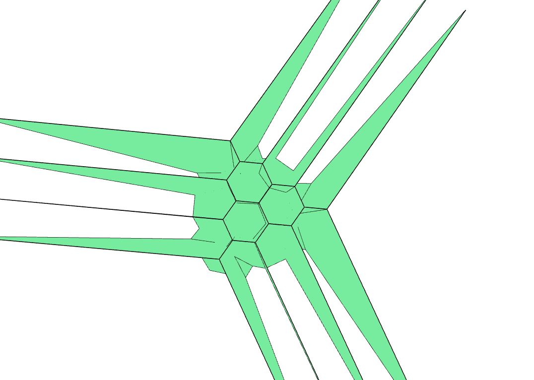
Figure 6.1. Compactified tropical $K3$-surface

Cellular (co-)sheaves in polymake are realised as EdgeMaps on the Hasse diagram. An EdgeMap is a map from the edges of a graph to some category. In our case, edges are mapped to maps of vector spaces, represented by matrices. Our extension for cellular sheaves can be found on github at https://github.com/lkastner/cellularSheaves. In its demo folder there are several Jupyter notebooks with commented examples on how to compute cohomology of cellular sheaves. Since the code is too long to display here, we will just briefly outline some examples.

Example .

The compactification of matroid fans explained in subsection 3.2 can be computed in polymake.

We revisit Example 5 of [KSW17] of the matroid of the so-called braid arrangement of lines in $\operatorname{\mathbb{C}P}^{2}$ , whose complement is the moduli space of 5-marked genus 0 curves $\mathcal{M}_{0,5}$, see [AK06]. This matroid is also the graphical matroid of the complete graph $K_{4}$. Below is the polymake code which produces the matroid fan and its compactification.

⬇

application "fan";

$g = graph::complete(4);

$m = matroid::matroid_from_graph($g);

$t = tropical::matroid_fan<Max>($m);

$t->VERTICES;

$matFan = new PolyhedralComplex($t);

$matFanComp = $matFan->COMPACTIFICATION;

print $matFanComp->nodes_of_rank(1)->size;

> 26

One can see that the compactification has $26=1+15+10$ vertices. The fan structure computed by polymake in this case is the coarsest structure of this fan, which corresponds to the minimal nested set compactification in the sense of [FS05]. Note that vertices correspond to nodes of rank $1$ by polymake’s projective viewpoint, i.e. the vertices of a polyhedral complex are the rays of the fan one gets by embedding said complex at height one. The following code gives a full comparison of the number of faces of fixed dimension, in other words the F-vectors, of the compactification and the original polyhedral complex:

⬇

for(my $i=1; $i<$matFanComp->rank; $i++){

print $matFanComp->nodes_of_rank($i)->size,"␣";

}

print "\n";

$matFanHasse = $matFan->HASSE_DIAGRAM;

$far = $matFan->FAR_VERTICES;

for(my $i=1; $i<$matFanHasse->rank; $i++){

my @faces = @{$matFanHasse->nodes_of_rank($i)};

@faces = map($matFanHasse->FACES->[$_], @faces);

@faces = grep(($_*$far)->size < $_->size, @faces);

print scalar @faces,"␣";

}

> 26 40 15

> 1 10 15

Note that due to polymake considering a polyhedral complex as a fan, one gets faces consisting only of far vertices. To get to the actual F-vector, these have to be removed.

We can then use a loop to assemble the cosheaves for the tropical homology on the compactification, build their associated chain complexes and finally to compute their dimensions.

⬇

@rows = ();

for(my $i=0; $i<=$matFan->DIM; $i++){

my $f = $matFan->compact_fcosheaf($i);

my $d = build_full_chain($matFanComp, $matFanComp->ORIENTATIONS, $f->BLOCKS, false);

push @rows, new Vector<Int>(topaz::betti_numbers($d));

}

print new Matrix(\@rows);

> 1 0 0

> 0 5 0

> 0 0 1

We see from the calculation that the tropical homology groups of the compactified matroid fan have the same Betti numbers as $\overline{\mathcal{M}_{0,5}}$, which is the blow up of $\operatorname{\mathbb{C}P}^{2}$ in four points. Therefore, the compactification we have computed is the minimal nested set compactification in the sense of [FS05]. The Chow group a of matroid with respect to a chosen nested set compactification is defined in [FY04]. Moreover, this can be generalised to any simplicial fan whose support is a matroid fan and the resulting Chow ring will satisfy Poincaré duality, Hard Lefschetz, and the Hodge Riemann bilinear relations [AP20].

The tropical homology of the fan prior to compactifying was computed in Example 5 of [KSW17]. This computation provides the duals of the graded pieces of the Orlik-Solomon algebra of this matroid.

Example (Hodge numbers of a K3).

Figure 6.1 shows a compactified K3 surface $\overline{X}$ in the tropical toric variety $\mathbb{T}P^{3}$. The boundary of $\overline{X}$ consists of $4$ quartic tropical curves, one corresponding to each face of the size $3$ standard simplex. The dimensions of the tropical homology groups correspond to the Hodge numbers of a complex K3 surface. Computing the dimensions of the tropical homology groups on the non-compact polyhedral complex one arrives at

⬇

0 0 34

0 31 3

1 0 1

or its transpose. On the compactification, we arrive at the proper Hodge diamond:

⬇

> print hodge_numbers($k3);

1 0 1

0 20 0

1 0 1

Of course this Hodge diamond has been known for some time, this example just serves to give a glimpse at possible future computations.

Remark .

In section 6 the computation of a signed incidence relation was already done in the background. In polymake this is realised as an EdgeMap on the Hasse diagram, labeling every edge with $\pm 1$. One can access this property as ORIENTATIONS on both the HASSE_DIAGRAM and the COMPACTIFICATION. Due to the encoding it is not trivial to make sense of the output. The nodes of the different Hasse diagrams are numbered, the same is true for the edges, so to go backwards one first needs to translate the index of an edge into its endpoints, and then these endpoints back into faces.

Example .

In [RS18] the $\mathbb{Z}_{2}$-Betti numbers of the real part of a hypersurface in a non-singular toric variety obtained by a primitive patchworking are equal to the Betti numbers of the sign cosheaf on the associated tropical variety equipped with a real phase structure. The main result of [RS18] is to bound the Betti numbers of the real part of the hypersurface by sums of dimensions of the tropical homology groups.

These arguments apply to hypersurfaces in the torus and partially compactified (or compact) toric varieties. In the partially compactified (or compactified) case one must work with the homology of the sign cosheaf on the closure of the tropical variety. The extension of the sign cosheaf to the compactification of tropical hypersurfaces in toric varieties has also been implemented in our extension. The following is an example of a degree three curve in two-dimensional tropical projective space, also using polymake’s patchworking framework [JV20].

⬇

$g = toTropicalPolynomial("min(3*x_0,2*x_0+x_1,2*x_0+x_2,927+x_0+2*x_1,351+x_0+x_1+x_2,30+x_0+2*x_2,2856+3*x_1,1884+2*x_1+x_2,942+x_1+2*x_2,411+3*x_2)");

$trop = new Hypersurface<Min>(POLYNOMIAL=>$g);

# Print the monomials, as they might get reordered inside the hypersurface.

print $trop->COMPACTIFICATION->DECORATION;

> ({} 0 {} {})

> ({0} 1 {0 11} {0})

> ({1} 1 {0 8} {0})

> ({2} 1 {2 10} {2})

> ({3} 1 {0 9} {0})

> ({4} 1 {1 9} {1})

> ({5} 1 {2 4} {2})

> ({6} 1 {1 6} {1})

> ({7} 1 {2 3} {2})

> ({8} 1 {1 3} {1})

> ({9} 1 {11} {})

> ({10} 1 {8} {})

> ({11} 1 {10} {})

> ({12} 1 {9} {})

> ({13} 1 {7} {})

> ({14} 1 {5} {})

> ({15} 1 {6} {})

> ({16} 1 {4} {})

> ({17} 1 {3} {})

> ({0 9} 2 {0 11} {})

> ({1 10} 2 {0 8} {})

> ({2 11} 2 {2 10} {})

> ({3 12} 2 {0 9} {})

> ({4 12} 2 {1 9} {})

> ({5 16} 2 {2 4} {})

> ({6 15} 2 {1 6} {})

> ({7 17} 2 {2 3} {})

> ({8 17} 2 {1 3} {})

> ({9 11} 2 {10 11} {})

> ({9 13} 2 {7 11} {})

> ({10 12} 2 {8 9} {})

> ({10 13} 2 {7 8} {})

> ({11 14} 2 {5 10} {})

> ({13 15} 2 {6 7} {})

> ({14 15} 2 {5 6} {})

> ({14 16} 2 {4 5} {})

> ({16 17} 2 {3 4} {})

> ({-1} 3 {-1} {})

$pw = $trop->PATCHWORK(SIGNS=>[1,0,1,1,1,1,1,1,1,1]);

$cosheaf = $pw->sign_cosheaf();

$comp = $trop->COMPACTIFICATION;

$chain = fan::build_full_chain($comp, $comp->ORIENTATIONS, $cosheaf, true);

print topaz::betti_numbers<GF2>($chain);

> 2 2

Example (Smooth tropical cubic).

A smooth tropical cubic corresponds to a regular unimodular triangulation of the dilated simplex $3\cdot\Delta_{3}$. Just as in section 6 one can compute the Betti numbers of the real cubic via patchworkings and cellular sheaves:

⬇

> print topaz::betti_numbers<GF2>($chain);

1 7 1

References

- [AP20] Omid Amini and Matthieu Piquerez “Hodge theory for tropical varieties”, 2020 arXiv:2007.07826 [math.AG]
- [AK06] Federico Ardila and Caroline J. Klivans “The Bergman complex of a matroid and phylogenetic trees” In J. Combin. Theory Ser. B 96.1, 2006, pp. 38–49 DOI: 10.1016/j.jctb.2005.06.004
- [Bez+17] Jeff Bezanson, Alan Edelman, Stefan Karpinski and Viral B Shah “Julia: A fresh approach to numerical computing” In SIAM review 59.1 SIAM, 2017, pp. 65–98 URL: https://doi.org/10.1137/141000671
- [BS11] José Ignacio Burgos Gil and Martín Sombra “When do the recession cones of a polyhedral complex form a fan?” In Discrete Comput. Geom. 46.4 Springer US, New York, NY, 2011, pp. 789–798
- [Cur13] Justin Curry “Sheaves, Cosheaves and Applications”, 2013 arXiv:1303.3255 [math.AT]
- [FS05] Eva Maria Feichtner and Bernd Sturmfels “Matroid polytopes, nested sets and Bergman fans” In Port. Math. (N.S.) 62.4, 2005, pp. 437–468
- [FY04] Eva Maria Feichtner and Sergey Yuzvinsky “Chow rings of toric varieties defined by atomic lattices” In Invent. Math. 155.3 Springer, Berlin/Heidelberg, 2004, pp. 515–536
- [Gan10] Bernhard Ganter “Two basic algorithms in concept analysis.” In Formal concept analysis. 8th international conference, ICFCA 2010, Agadir, Morocco, March 15–18, 2010. Proceedings Berlin: Springer, 2010, pp. 312–340
- [GJ00] Ewgenij Gawrilow and Michael Joswig “polymake: a framework for analyzing convex polytopes” In Polytopes—combinatorics and computation (Oberwolfach, 1997) 29, DMV Sem. Basel: Birkhäuser, 2000, pp. 43–73
- [HJS19] Simon Hampe, Michael Joswig and Benjamin Schröter “Algorithms for tight spans and tropical linear spaces.” In J. Symb. Comput. 91 Elsevier (Academic Press), London, 2019, pp. 116–128
- [Ite+16] Ilia Itenberg, Ludmil Katzarkov, Grigory Mikhalkin and Ilia Zharkov “Tropical Homology”, 2016 arXiv:1604.01838
- [JRS18] Philipp Jell, Johannes Rau and Kristin Shaw “Théorème de Lefschetz en géométrie tropicale” Id/No 11 In Épijournal de Géom. Algébr., EPIGA 2 Association de l’Épijournal de Géométrie Algébrique c/o Université de Lorraine, Institut Élie Cartan de Lorraine, Vandœuvre-lés-Nancy, 2018, pp. 27
- [JSS19] Philipp Jell, Kristin Shaw and Jascha Smacka “Superforms, tropical cohomology, and Poincaré duality” In Adv. Geom. 19.1 De Gruyter, Berlin, 2019, pp. 101–130
- [JL16] Michael Joswig and Georg Loho “Weighted digraphs and tropical cones.” In Linear Algebra Appl. 501 Elsevier (North-Holland), New York, NY, 2016, pp. 304–343
- [JV20] Michael Joswig and Paul Vater “Real tropical hyperfaces by patchworking in polymake”, 2020 arXiv:2003.06326 [math.CO]
- [KLT20] Marek Kaluba, Benjamin Lorenz and Sascha Timme “Polymake.jl: A New Interface to polymake” In Mathematical Software – ICMS 2020 Cham: Springer International Publishing, 2020, pp. 377–385
- [KSW17] Lars Kastner, Kristin Shaw and Anna-Lena Winz “Cellular sheaf cohomology in polymake.” In Combinatorial algebraic geometry. Selected papers from the 2016 apprenticeship program, Ottawa, Canada, July–December 2016 Toronto: The Fields Institute for Research in the Mathematical Sciences; New York, NY: Springer, 2017, pp. 369–385
- [MS15] Diane Maclagan and Bernd Sturmfels “Introduction to tropical geometry.” In Grad. Stud. Math. 161 Providence, RI: American Mathematical Society (AMS), 2015, pp. xii + 363
- [Mik04] Grigory Mikhalkin “Amoebas of algebraic varieties and tropical geometry.” In Different faces of geometry New York, NY: Kluwer Academic/Plenum Publishers, 2004, pp. 257–300
- [Mik04a] Grigory Mikhalkin “Decomposition into pairs-of-pants for complex algebraic hypersurfaces.” In Topology 43.5 Elsevier Science Ltd (Pergamon), Oxford, 2004, pp. 1035–1065
- [MR] Grigory Mikhalkin and Johannes Rau “Tropical Geometry” Book, draft available at https://math.uniandes.edu.co/~j.rau/downloads/main.pdf
- [OR13] Brian Osserman and Joseph Rabinoff “Lifting nonproper tropical intersections.” In Tropical and non-Archimedean geometry. Bellairs workshop in number theory, tropical and non-Archimedean geometry, Bellairs Research Institute, Holetown, Barbados, USA, May 6–13, 2011 Providence, RI: American Mathematical Society (AMS); Montreal: Centre de Recherches Mathématiques, 2013, pp. 15–44
- [Pay09] Sam Payne “Analytification is the limit of all tropicalizations” In Math. Res. Lett. 16.3, 2009, pp. 543–556 DOI: 10.4310/MRL.2009.v16.n3.a13
- [Rab12] Joseph Rabinoff “Tropical analytic geometry, Newton polygons, and tropical intersections.” In Adv. Math. 229.6 Elsevier (Academic Press), San Diego, CA, 2012, pp. 3192–3255
- [RS18] Arthur Renaudineau and Kristin Shaw “Bounding the Betti numbers of real hypersurfaces near the tropical limit”, 2018 arXiv:1805.02030 [math.AG]
- [RST05] Jürgen Richter-Gebert, Bernd Sturmfels and Thorsten Theobald “First steps in tropical geometry” In Idempotent mathematics and mathematical physics 377, Contemp. Math. Amer. Math. Soc., Providence, RI, 2005, pp. 289–317 DOI: 10.1090/conm/377/06998
- [Spe04] David Speyer “Tropical Linear Spaces” In SIAM Journal on Discrete Mathematics 22, 2004, pp. 1527–1558 DOI: 10.1137/080716219
- [Tev07] Jenia Tevelev “Compactifications of subvarieties of tori” In Am. J. Math. 129.4 Johns Hopkins University Press, Baltimore, MD, 2007, pp. 1087–1104