Numerical approximation of singular-degenerate parabolic stochastic PDEs
Abstract.
We study a general class of singular degenerate parabolic stochastic partial differential equations (SPDEs) which include, in particular, the stochastic porous medium equations and the stochastic fast diffusion equation. We propose a fully discrete numerical approximation of the considered SPDEs based on the very weak formulation. By exploiting the monotonicity properties of the proposed formulation we prove the convergence of the numerical approximation towards the unique solution. Furthermore, we construct an implementable finite element scheme for the spatial discretization of the very weak formulation and provide numerical simulations to demonstrate the practicability of the proposed discretization.
1. Introduction
In this paper we study the numerical approximation of a class of singular-degenerate parabolic stochastic partial differential equations
| (1) |
where , is a bounded, open domain and is a multiplicative noise term which will be specified below.
The above equation for is the stochastic porous medium equation and for the equation corresponds to the stochastic fast diffusion equation; the case yields the stochastic heat equation.
Stochastic quasilinear diffusion equations of the type (1) appear in several contexts, including, interacting branching diffusion processes [10], self-organized criticality [2, 33], and non-equilibrium fluctuations in non-equilibrium statistical mechanics [27, 20]. We next present three of such instances in more detail.
As a first example, consider the gradient flow structure of the porous medium equation
with Onsager operator and energy . The corresponding fluctuating system, in accordance with the GENERIC framework of non-equilibrium thermodynamics (see [51]), then reads
| (2) | ||||
| (3) |
with , the Boltzmann constant and a vector-valued space-time white noise. Notably, the stochastic PDE (3) is super-critical and, thus, lacks a well-posedness theory. The results of the present paper are applicable to approximate versions of (3), that is, to
| (4) |
where is a trace-class Wiener process in ; in this case, in one spatial dimension, the stochastic perturbation still is less-regular than space-time white noise.
The second class of examples arises from fluctuations in non-equilibrium statistical mechanics. This leads to stochastic PDE of the general type
| (5) |
where denotes space-time white noise, with the Dean-Kawasaki stochastic PDE
as a model example, see for example [15, 45, 21]. Stochastic PDE of this type serve as continuum models for interacting particle systems, including stochastic corrections reproducing the correct fluctuation behavior on the central limit and large deviations scale, see [19]. Since for large particle number the fluctuations decay, we see the small factor in front of the noise. For example, a concrete example of an interacting particle process is given by the zero range process, see [27, 28], leading to nonlinear, non-degenerate diffusion in (5) and noise coefficients corresponding to . We note that with this choice (5) is in line with the GENERIC framework (2) when considering
| (6) |
as a gradient flow on the space of measures with energy given by the Boltzmann entropy. The corresponding stochastic PDE (5) is super-critical and, therefore, lacks a well-posedness theory. Instead, one considers joint scaling limits of
| (7) |
where is a regularized noise, see [28, 27]. In the case and Lipschitz continuous, this class of stochastic PDE is included in the results of the present work.
The third class of equations covered by the present work arises in the continuum scaling limit of the empirical mass of interacting branching diffusions with localized interaction, which, informally, converges to the solution of a stochastic PDE
| (8) |
where denotes space-time white noise, see [9, 49]. The results of the present work apply to the particular case of and being a trace class Wiener process in .
It is common to these stochastic PDE that, due to the irregularity of the random perturbation, solutions are expected to be of low regularity. In fact, in many cases solution take values in spaces of distributions only, causing severe difficulties in even giving meaning to the nonlinear terms appearing in the stochastic PDE.
The lack of regularity of solutions is one of the decisive differences distinguishing the numerical analysis of stochastic PDE from deterministic PDE. While, if the noise and thus the solutions are regular enough, the numerical analysis can proceed similarly to the deterministic case, this ceases to be true in more rough situations. Indeed, if one considers (1) with regular enough noise, the solutions will take values in spaces of functions ( spaces), and, therefore, standard finite element basis can be used, such as piecewise constant or piecewise linear functions. The proof of their convergence still requires adaptation from the deterministic arguments, e.g. replacing compactness arguments by a combination of tightness arguments and Skorohod’s representation theorem (cf. e.g. [38]), but the numerical method is close to the deterministic case. In contrast, when the noise is not as regular, one cannot expect to close -based estimates, but one has to work in spaces of distributions. Concretely, this means to move from -based estimates for (1) to -based estimates.
While the modification of finite element methods from -based to -based thus is necessary and natural in the context of stochastic PDE, this causes obstacles in their numerical realization: Precisely, while in an -based approach, the choice of piecewise constant (or piecewise linear) finite elements leads to a sparse mass matrix
this is not true in the -based approach which leads to a mass matrix
| (9) |
Note that (9) is not a sparse matrix, since has global support. Consequently, the resulting numerical scheme is inefficient.
Interestingly, in one spatial dimension this difficulty was addressed in the contribution [24], where an -based finite element scheme was suggested in the context of a deterministic porous medium equation, motivated by the aim to treat irregular initial data and forcing. In [24] it was noticed, that in one spatial dimension a modified finite element basis can be constructed, leading to a sparse mass-matrix (9). In view of (9) this requires to choose a basis so that has small support. While, in one spatial dimension, this can relatively easily be enforced by choosing of the form
for this construction becomes less obvious. In addition, in higher dimension, the proof of the -density of the resulting finite element spaces proves much more challenging.
In the light of this exposition, the contribution of the present work is two-fold: Firstly, motivated by the intrinsic irregularity of stochastic PDE, we provide an based analysis of a fully discrete finite element scheme for (1) and prove its convergence. Secondly, we construct a finite element basis in dimension , which allows for an efficient implementation of the proposed numerical approximation in the -setting, and analyze its approximation properties in . More precisely, motivated by the deterministic numerical approximation [24] we propose a fully discrete finite element based numerical approximation of (1) based on its very weak formulation. We show that the proposed numerical approximation converges for . Furthermore, we generalize the finite element spatial discretization of the very weak formulation, which was restricted to in [24], to higher dimensions. Moreover, we present numerical simulations to demonstrate the efficiency and convergence behavior of the proposed numerical scheme.
The paper is organized as follows. In Section 2 we state the notation and assumptions along with the definition and basic properties of very weak solutions of (1). We introduce the fully discrete numerical approximation of (1) in Section 3 and show well-posedness of the proposed discrete approximation along with a priori estimates for the numerical solution. The convergence of the numerical approximation towards the very weak solution of (1) is shown in Section 4. In Section 5 we propose and analyze a non-standard finite element scheme for the spatial discretization of the very weak solution which enables an efficient implementation of the resulting fully discrete numerical approximation. Numerical simulations which demonstrate the practicability of the proposed numerical scheme are presented in Section 6.
Comments on the literature
There exists a rich literature on the numerical approximation of deterministic degenerate parabolic equations, i.e. (1) with , where the earlier results include [48], [42]. For more recent results we refer to [23], [24], [18], [22] and the references therein. As far as we are aware, the only result on the numerical approximation of (1) so far is [38], where the convergence of the proposed numerical approximation towards a martingale solution has been shown in dimension for regular noise and a limited range of the exponent , not including the case of the stochastic fast diffusion equation.
In the deterministic setting, the analysis of the equation (1) is well understood, see, e.g. [57]. In the stochastic setting, the well-posedness of (1) in the variational framework goes back to [44, 52] with many details given in [47]; for a generalization of the variational approach to the case of the stochastic fast diffusion equation we refer to [53]. Generalizations to maximal monotone nonlinearities and Cauchy problems can be found in [3], based on monotonicity techniques. Martingale solutions for diffusion coefficients given as Nemytskii operators have been constructed in [37]. In [43] the well-posedness for (1) with additive noise was shown based on a weak convergence approach. An -based alternative approach to well-posedness has been developed based on entropy solutions in [6, 9, 13] and based on kinetic solutions in [35, 17, 34, 26, 28]. Solutions to (1) with space time white multiplicative noise have been constructed in [11].
Besides well-posedness, also the long-time behavior of solutions has been analyzed, see, for example, [26] for the existence of random dynamical systems, [7, 32] for the existence of random attractors, and [3, 14, 58] for ergodicity. For regularity of solutions we refer to [30, 16, 12, 4] and the references therein. Results on finite speed of propagation and waiting times were derived in [31, 3, 29]. Extensions to parabolic-hyperbolic SPDE may be found in [5, 6], and to doubly nonlinear SPDE in [54] and the references therein.
2. Notation and preliminaries
Let be a bounded open domain with -smooth boundary or a rectangular domain. For , we denote the conjugate exponent as . We use the notation for the standard Lebesgue spaces of -th order integrable functions on and for the standard Sobolev spaces on , where stands for the space with zero trace on ; for we denote the corresponding Sobolev spaces as and . We note that the dual space of , denoted by , is a Hilbert space with the scalar product where is the inverse Dirichlet Laplace operator .
Throughout the paper we denote , and and note that constitutes a Gelfand triple for the considered range of the exponent in (for one may take ), cf., [46].
For we define the inverse Laplace operator as the unique weak solution of the problem
| (10) | ||||
We note that the above assumption on guarantees that for and that depends continuously on .
We consider to be a cylindrical Wiener process on a real separable Hilbert space , that is, for an orthonormal basis of , we (formally) have with independent Brownian motions on a filtered probability space . Let denote the space of real Hilbert-Schmidt linear operators from to . We note that (, , ) is a real separable Hilbert space with inner product
and the corresponding norm .
We consider a slight generalization of the equation (1):
| (11a) | |||||
| (11b) | |||||
| (11c) | |||||
where , and ; the initial condition is assumed to be -measurable.
To simplify the presentation we consider (progressively measurable) and , a generalization to less regular data is straightforward, cf. [24]. Furthermore, we assume that the function is continuous, monotonically increasing, and satisfies a coercivity and growth condition, i.e.,
| (12) |
for some and , , , respectively.
Clearly, yields the stochastic porous medium/fast diffusion equation (1) and satisfies the above assumptions for .
We note that for by standard elliptic regularity theory, cf. [36, Ch. 9], [39, Ch. 4]. Furthermore, for the normal trace of satisfies for domains with -smooth boundary or rectangular domains, cf. [50, Thm. 5.4-5.5 p. 97-99]. Hence, it follows that . In the particular case the following also generalizes to convex domains with piecewise smooth boundary.
Throughout the paper we assume that the following conditions are satisfied.
Assumption 1.
-
i)
Hemi-continuity of : the function
is continuous for all .
-
ii)
Monotonicity of : there exists , such that for all
(13) -
iii)
Coercivity of : for and it holds
(14) -
iv)
Boundedness of : there exists a such that
We next generalize the concept of very weak solutions for the deterministic version of (11) with from [24] to the stochastic problem. We consider the integral form of (11) as
We multiply the above equation by , integrate over , and integrate twice by parts in the second order term to obtain, using the boundary condition,
The above formal construction motivates the following definition of very weak solutions of the stochastic problem (11).
Definition 2.1.
Let . Then a -adapted process is a very weak solution of (11) if it satisfies -a.s. for all and all :
| (15) |
with
| (16) |
Remark 2.2.
Owing to the Assumption 1 we may interpret the very weak formulation of (11) from Definition 2.1 as a monotone stochastic evolution equation posed on the Gelfand triple , cf. [46, Théorème 3.1], [24]. Hence, the existence and uniqueness of the very weak solution in Definition 2.1 follows by the standard theory of monotone stochastic evolution equations [44], [53].
Below we state examples of SPDE problems covered by the framework of Assumption 1; these include all of the problems mentioned in the introduction, in particular. We let be an orthonormal basis of consisting of eigenvectors of the Laplacian with Dirichlet boundary conditions and corresponding eigenvalues . We note that
| (17) |
Example 2.1 (GENERIC framework for the -gradient flow).
Example 2.2 (Fluctuations in non-equilibrium systems).
We consider (7) so that satisfies for some , is Lipschitz continuous and is a -valued Brownian motion, that is,
for , where . We choose , , , extended to , and
We then have
The remaining assumptions can be verified similarly. We note that the scaling relation implicitly depends on the dimension , since the number of frequency modes depends on the dimension, cf. [19].
Example 2.3 (Branching interacting particle systems).
We consider (8) with and is a trace-class Wiener process in , that is,
| (18) |
with and non-negative initial condition . In order to fit this example in the abstract setup of Assumption 1 we choose , , . Let be a cylindrical Wiener process on , extended to , and
where , satisfy . Note that then defines a trace class Wiener process in . We then have, by (17),
The remaining assumptions can be verified similarly.
3. Fully discrete Numerical Approximation
We introduce a uniform partition of the time interval with a constant time-step size , where , as with . For a mesh size we consider a family of finite dimensional subspaces with the approximation property
| (19) |
and let for any . We define a family of mappings via the best approximation property, i.e., for . Furthermore, we denote by the family of projection operators which satisfy
An explicit construction of the discrete finite element spaces and the operators and will be provided in Section 5 below (see Lemma 5.3, Corollary 5.4 and Remark 5.5).
We define the discrete Brownian increments for as
| (20) |
and for we define the truncated Hilbert-Schmidt operator as
where is the orthonormal basis of and .
The time-discrete approximation of the right-hand side (given in Definition 2.1) is obtained as
Given , , and , the fully discrete approximation of (11) is obtained as follows: set , and for determine as the solution of the problem
| (21) |
for all . We note that the above scheme can be equivalently rewritten as
| (22) | ||||
Remark 3.1.
We note that the choice , in (20) is not strictly required but is convenient since it slightly simplifies the notation and convergence analysis in Section 4 for . In particular, this choice enables to restate the numerical scheme (22) in the form (26) with the ”shifted” interpolant defined in (25) which satisfies the estimate in Corollary 4.1.
The measurability of the fully discrete solution is a consequence of the following lemma, c.f. [24, Lemma 3.2], [41, Lemma 3.8].
Lemma 3.2.
Let be a measure space. Let be a function that is continuous in its first argument for every (fixed) and is -measurable in its second argument for every (fixed) . If for every the equation has a unique solution then is -measurable.
The next lemma guarantees the existence, uniqueness and measurability of the fully discrete numerical approximation (21).
Lemma 3.3.
For any , , and there exists a unique solution of the numerical scheme (21). Furthermore, the -valued random variables are -measurable, .
Proof.
We assume that for there exist -valued random variables that satisfy (21) and that are -measurable for . We show the existence of -valued , that satisfies (21) and is -measurable.
For each the scheme (21) defines a canonical mapping for which it holds . Consequently for we write
We note that
Hence, using the coercivity Assumption 1 iii) along with the embedding we obtain
We choose such that
Since , we get for that
Consequently, for each the existence of that satisfies (21) follows by the Brouwer’s fixed point theorem [55, Ch. II, Lemma 1.4].
To show uniqueness we consider , , such that and obtain by the monotonicity Assumption 1 ii) that
which yields the uniqueness of the discrete solution for .
Finally, the -measurability of the follows by Lemma 3.2
∎
Under a slightly stronger assumption on we obtain the following stability Lemma.
Lemma 3.4.
For there exist constants , such that for it holds
and
Proof.
i) We set in (21) with , use the identity and by summing up the resulting equations for we get, that
| (23) |
Using the Cauchy-Schwarz and Young’s inequalities we estimate the stochastic term as
On noting the independence of and we estimate
Next, on recalling (2.1), using the boundedness of , we deduce by the Hölder and Young inequalities that
Hence, on recalling the coercivity Assumption 1 and using the above inequalities we obtain after taking the expectation in (3) that
The first statement of the Lemma then follows after an application of the discrete Gronwall lemma for .
ii) For the second estimate we use the boundedness Assumption 1 , and obtain that
Hence the second estimate follows by part of the proof. ∎
Remark 3.5.
The assumption on the step-size in the above Lemma (which is required for the application of the discrete Gronwall lemma) is not too restrictive. For instance, for the stochastic porous media equation (1) with one may deduce for the constants in Assumption 1, (13) that , , . Consequently, we only require a mild condition .
4. Convergence of the numerical approximation
Given the temporal partition with associated discrete random variables we define the piecewise constant time-interpolants for as follows:
| (24) |
and
| (25) | ||||
We note that the interpolant is adapted by Lemma 3.3.
On recalling (22) we note that the numerical scheme can be restated in terms of the above interpolants, i.e., it holds -a.s. that
| (26) |
where
| (27) |
As a consequence of Lemma 3.4 and Assumption 1 the time interpolants from (24) and (25) satisfy the following a priori estimates.
Corollary 4.1.
For any and (sufficiently small) it holds that
and
where is a constant that only depends on the data of the problem.
From the a priori bounds in Corollary 4.1 we can directly deduce the following sub-convergence result.
Lemma 4.2.
Let the Assumptions 1 hold and let . Then there exists a subsequence (not relabeled) such that for , the following holds:
-
i)
there is a progressively measurable such that
There is a such that
-
ii)
There exists a progressively measurable such that in . There is a progressively measurable such that , and weakly converge to in .
-
iii)
for -almost all the following equation holds in
(28) -
iv)
there is an -valued continuous version of (sill denoted by ) which satisfies (28) and
(29) -
v)
, i.e. in .
Proof.
i) We deduce from Corollary 4.1 iii), iv) that and in . The limit are the same according to [25, Lemma 4.2] see also [40, proof of Prop. 3.3].
Item of the Lemma follows from Corollary 4.1 and , the limits again coincide in by the arguments from .
To show part we consider for , . We set with in (26), integrate w.r.t. over and take the expectation to get
| (30) | ||||
where
By the boundedness of and in and in and an application of Itô’s isometry we get , , for .
Further, the boundedness of in and in yields for that
On recalling and , we deduce by (19) that
Hence, on noting Corollary 4.1 we conclude that , for .
Next, the weak convergence , implies for ,
From the weak convergence of in and the strong convergence of in we deduce that
| and | |||
Finally, since in it follows that
From the above convergence results we conclude, by taking , in (30) that
for all , , which implies (28).
By the standard theory of monotone SPDEs, cf. [44] (or [53]), part follows from by the Itô formula for the square of the -norm, which also implies that has an -valued continuous modification (which we again denote by ) that satisfies (28).
Finally, to show we note that by part which together with implies
Since the continuous -valued modification of (cf. ) satisfies (28) we may conclude that . ∎
The following variant of the Gronwall lemma, cf. [25, Lemma 5.1], will be useful for the proof of the subsequent theorem.
Lemma 4.3.
In the next theorem we conclude that the weak limit of the numerical approximation from Lemma 4.2 is the very weak solution of the equation (11).
Theorem 4.4 (Convergence of the numerical approximation).
Proof.
We have shown in Lemma 4.2 that every weak limit of the numerical approximation satisfies for
Hence, it remains to show that , .
Throughout the proof we use the shorthand notation and stands for , . We define
Analogously to the proof of Lemma 3.4 we deduce from (3) on noting the definition of the time interpolants (26) that for any it holds
with .
We use Lemma 4.3 and obtain from the above inequality that
| (33) | |||
Note that by the monotonicity property (13) it holds for arbitrary that
We substitute the above inequality into (33) and obtain
| (34) | |||
Next, we observe that, by Corollary 4.1,
Hence, using the weak convergence of Lemma 4.2 i), ii) we deduce from (34) by the lower-semicontinuity of norms that
| (35) | |||
After a standard stopping argument and taking the expectation in (29) we get for all
Using Lemma 4.3 we obtain from the above equality that
| (36) |
Next, we subtract (36) from (35) and get
Consequently, it holds that
| (37) |
On taking in (37) we get
which implies in .
Next we choose (37) with ,
and obtainusing Assumption 1 i) by the Lebesgue dominated convergence for that
This implies that , since is arbitrary.
Finally, we conclude by the uniqueness of the very weak solution, that the whole sequence converges to the same limit .
∎
5. Practical finite element approximation in
A natural approach is to construct the numerical solution , using a finite element space consisting of piecewise constant functions on a given partition of the domain with a given mesh size . However, the piecewise constant finite element approximation of the very weak formulation is impractical since the resulting finite element matrix associated with the -scalar product in the discrete very weak formulation (21) will be dense. Furthermore, the evaluation of the -inner product requires the evaluation of the inverse Laplace operator , which does not have an explicit formula in general. This is a consequence of the fact that the inverse Laplacian of the characteristic function for some subset does not have compact support in , i.e., in general . A further complication lies in the fact that there is no explicit formula available for , in general.
Below, we discuss the construction of a finite element basis of for on rectangular domains with the property that can be computed explicitly and has local support in for .
5.1. Finite-element basis in
We summarize the finite element method proposed in [24] for . For the domain , where we introduce a partition into disjoint open intervals , , such that and denote to be the characteristic function of the interval . We then set where are defined as
| (38) | ||||
| (39) | ||||
| (40) |
for any .
Note that the proposed approximation is equivalent to a piecewise constant approximation, i.e., . The proposed basis has the useful property that (with defined on ) admits an explicit representation for all which has a small support in . It can be verified by direct calculation that
| (41) |
further
| (42) |
for , and
| (43) |
We note that both basis have a small support in , i.e., , with
Consequently, the ”mass” matrix
which corresponds to the -inner product in the numerical scheme (21) will be sparse.
5.2. Spatial discretization in higher dimensions
We consider for some , , and denote . Given we set and consider a uniform partition of with mesh size into rectangular subdomains for a multiindex , where , for , and . We denote the above partition of the domain as .
We consider , , to be the one dimensional basis functions defined in the previous section and construct the basis functions , of in as follows: for we set
| (44) | ||||
On noting it can be deduced from (44) by a direct calculation that can be expressed explicitly as
| (45) | ||||
Equivalently the basis functions , are the solutions of the Poisson problem
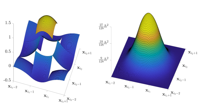
An example of a basis function for for is given in Figure 1.
Clearly since for all . In addition, since , have a small local support in , also and remain ”small”. Consequently, the "mass" matrix for
is sparse; more precisely, there are only non-zero elements in each row of .
By construction, the finite element space consists of (discontinuous) piecewise polynomial functions on the rectangular partition of the domain . In order to analyze the approximation properties of in it is convenient to consider the space of piecewise constant functions on which is denoted as where .
We define the restriction operator as
| (46) |
where .
Next we analyze the properties of the operator .
Lemma 5.1.
For any the operator is -stable, i.e., for all , and for all it holds that
Proof.
The -stability follows from the definition of by the Hölder inequality as
Next, we assume that is smooth, the result for follows by density. By the fundamental theorem of calculus and the Hölder inequality we get that
∎
Lemma 5.2.
is a Galerkin scheme for , . I.e., for every it holds that
Proof.
For the (piecewise polynomial) basis functions defined in (44) we denote and observe that .
In order to show the approximation property of the finite element space we define the restriction operator as
| (48) |
where .
For simplicity we restrict the proof of the convergence of the above restriction operator to and assume that is a rectangle; we expect an analogous proof to hold for and more general domains as well. For we denote by the finite-dimensional space spanned by the the first eigenfunctions of the homogeneous Dirichlet Laplace operator on the rectangular domain
| (49) |
By the density of in it suffices to show the convergence of the restriction operator (48) for .
Lemma 5.3.
Let be fixed. For any and it holds that
Proof.
It is enough to show that the statement holds for , .
For we consider the following discrete Laplace operator
| (50) | ||||
The discrete Laplace operator corresponds to the 9-point finite difference approximation of the Laplace operator, cf. [8, p. 190, Example 4]; see also Figure 2.

We note that for the discrete Laplace operator (50) satisfies the consistency property
| (51) |
With each element we associate the corresponding basis functions , . To deal with the complication that the basis functions associated with the elements of the partition along the boundary of the domain have a different shape (c.f., (44) for and (38), (40)), we introduce a layer of ”ghost” cells , , , , (the dimensions of the cells will be specified below) along the outer side of the boundary of . We then denote the resulting extended partition with cells as , i.e., includes the elements of and the ”ghost” cells.
Recall the following trivial symmetry properties of the eigenfunctions from (49) (as well as for , since ) which hold along the boundary of : , , and , . We note that (for ghost cells with dimensions given implicitly via the definition (53)) the symmetry also transfers to the piecewise constant approximation of over , i.e., for naturally extended on . We will use this fact to construct an "extension" of from (48) on (see (55) below).
We consider a (modified) finite element basis associated with the elements of the extended partition with basis functions which are defined as (44) with the exception that we only use the (suitably shifted) "interior" basis functions (39), (42). Namely, we use (44) where for , we set for
| (52) |
where we define , (i.e., we replace the basis functions (38), (40) and (41), (43) by their "interior" counterparts); we proceed analogously for the basis functions , , i.e., replace (41), (43) by a suitably shifted analogues , of (42).
We note that the ”boundary” basis functions satisfy , (and similarly for , ). We deduce from (44) that analogous relations also hold for and (as well as for and ) for instance it holds at the bottom boundary (analogically for the top, left and right boundaries)
| (53) |
and similarly for , . Slightly modified relations hold for the basis functions associated with the corner elements , , , of ; for instance for we deduce
| (54) | ||||
and similarly for basis functions at , , .
On noting the aforementioned symmetry properties of eigenfunctions and the relations (53), (54) (along with their counterparts covering the remaining situations) we observe that (48) for is equivalent to
| (55) |
where is the previously constructed extended basis of "interior" basis functions associated with elements of .
The equivalent representation (55) of the restriction operator (48) simplifies the subsequent considerations, since it only involves one type of (interior) basis functions. For the rest of the proof we will work with the basis functions but drop the superscript ”∗” to simplify the notation (also note for , i.e., the modification is only required at the boundary).
We consider an element . By a direct calculation of the elementwise mean of the basis functions (44) for (i.e., evaluating ), we note that for , fixed it holds that and for , , cf. Figure 2; below we denote the local index of with respect to and write . Consequently, we observe that the coefficients in the definition of the discrete Laplace operator (50) for correspond to the values , , scaled by the factor .
Hence, from the above observation, noting the definitions (48), (46) and recalling (50) we deduce for that
| (56) | ||||
where we employed the integral transformation for (i.e., ) along with the fact that .
By the consistency property (51) we get from (56) for that
Consequently, on recalling Lemma 5.1 we conclude for that
| (57) |
Next, we estimate the difference . Due to the local support of the basis functions for we may express
| (58) |
As in (56) we employ the transformation for and rewrite the above expression as
Hence, after expressing the basis functions (44) explicitly (recall , ), for each we restate
| (59) | ||||
where we employ a shorthand notation and for we denote (cf. (44))
The following property, which follows from (42) by direct calculation, will be essential in the sequel
| (60) |
for , and .
The above lemma allows us to deduce the density of in .
Corollary 5.4 (Approximation property of ).
For every , it holds that
Proof.
Consider and note that by Lemma 5.3. Since we get
The statement then follows by the density of in . ∎
The restriction operator (48) is not implementable since it requires the evaluation of the function , which is not available in general. For practical purposes (e.g., to compute the discrete approximation of the initial condition) it is convenient to consider the discrete -projection which is defined for as follows
| (64) |
Remark 5.5.
The -stability of the orthogonal projection, i.e., follows on taking in (64) and using the Cauchy-Schwarz and Young’s inequalities. Furthermore, we note that (64) is equivalent to which in particular implies that for .
Consequently, the -stability of and the continuous embedding , for yield for all ,
Hence, by Lemma 5.3, the density of , in and the density of in we conclude the approximation property of the -orthogonal projection:
6. Numerical Experiments
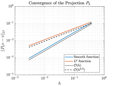
6.1. Convergence of the projection in
We study the experimental -convergence of the -projection operator (64) as well as of an implementable counterpart of the restriction operator (48) defined as
where . I.e., the coefficients are the solutions of finite difference scheme
for ; we note that it holds by construction that and .
In Figure 3 we display the convergence plot of the -projection of the Barenblatt solution at (see (65) below) along with the convergence plot of of the (non-smooth) indicator function of the -square; in both cases . The convergence plot implies convergence of the projection in of order for the smooth Barenblatt function and of order of in the non-smooth case.
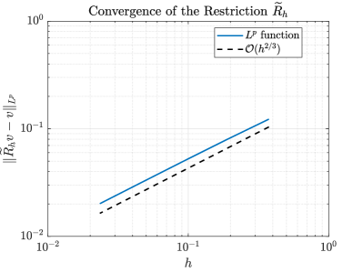
In addition we display in Figure 3 the convergence plot of the restriction operator for the indicator function which is also of order .
6.2. Barenblatt solution for the deterministic PME
We consider the equation (1) with , , , which corresponds to the deterministic porous medium equation
The exact solution of the porous media equation with initial condition (i.e., the -distribution centered at ) the so-called Barenblatt solution
| (65) |
where are suitable constants that depend on , , c.f. [57, Ch. 17.5].
In the experiments below we choose , and , . We consider a regularized initial condition with
and set .
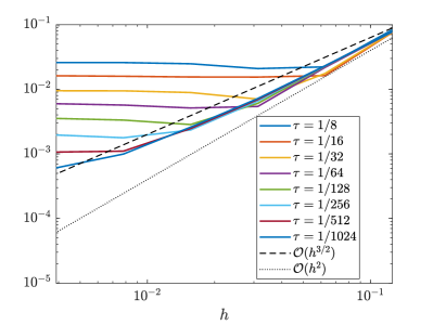
We examine the convergence of the numerical approximation with respect to , in the -norm, i.e., we compute the error with time-interval where we choose to reduce the effect of the approximation of the initial condition.
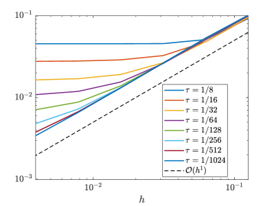
In Table 1 we display the -error for , in . The corresponding convergence plots in Figure 4 indicate that the convergence order of the numerical approximation with respect to is slightly less than one and around with respect to .
| 0.083032 | 0.02221 | 0.020881 | 0.024805 | 0.025878 | 0.025931 | |
| 0.07524 | 0.016254 | 0.015419 | 0.015481 | 0.015893 | 0.016162 | |
| 0.075711 | 0.017544 | 0.0070398 | 0.0088919 | 0.0094508 | 0.0094772 | |
| 0.077172 | 0.021771 | 0.0054151 | 0.0051293 | 0.0056912 | 0.0059705 | |
| 0.077702 | 0.022649 | 0.0060452 | 0.0028429 | 0.0033319 | 0.0035322 | |
| 0.077591 | 0.022801 | 0.006569 | 0.002342 | 0.0017761 | 0.0019579 | |
| 0.077532 | 0.022934 | 0.0069462 | 0.002467 | 0.0011016 | 0.0010656 | |
| 0.077593 | 0.023061 | 0.007187 | 0.0025917 | 0.00099377 | 0.00060724 |
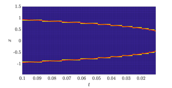
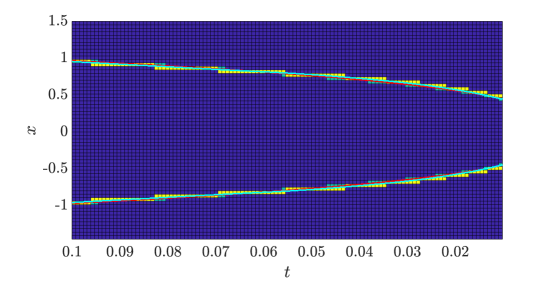
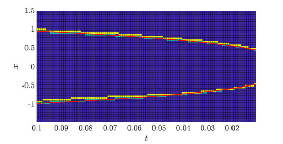
To highlight the finite speed of propagation property on the discrete level we display the evolution of the support of the numerical approximation in Figure 5.

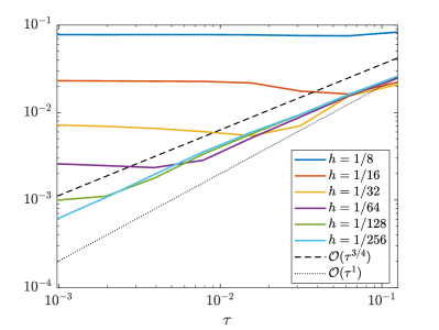
Next we examine the convergence behaviour in , we note that in this case . In Table 2 we display the -error computed for , .
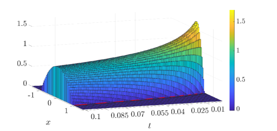
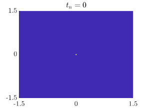
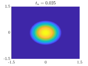
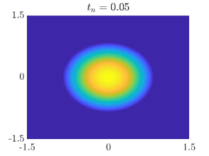
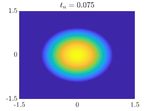
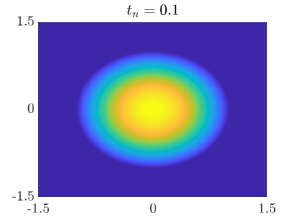
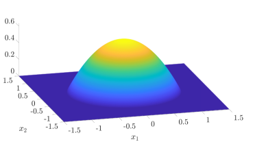
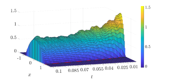
The corresponding convergence plots in Figure 6 indicate that the convergence order of the numerical approximation with respect to and are both close to one. As expected, (due to the lower regularity of the initial condition in ) the observed convergence order of the spatial discretization is slightly worse than the corresponding convergence order for . We display the time evolution of the numerical solution in Figure 7 and a detail of the numerical solution at , is displayed in Figure 8.
| 0.092154 | 0.050998 | 0.045512 | 0.04534 | 0.04531 | 0.045288 | |
| 0.094038 | 0.047956 | 0.032504 | 0.028832 | 0.027894 | 0.027644 | |
| 0.095218 | 0.048104 | 0.026604 | 0.019108 | 0.016976 | 0.016402 | |
| 0.098787 | 0.050731 | 0.026017 | 0.015466 | 0.011883 | 0.010852 | |
| 0.10062 | 0.052414 | 0.026237 | 0.013883 | 0.0087862 | 0.0070965 | |
| 0.10077 | 0.052773 | 0.026229 | 0.013247 | 0.0072316 | 0.0048007 | |
| 0.10086 | 0.052981 | 0.026295 | 0.013092 | 0.0067107 | 0.0037732 | |
| 0.10109 | 0.05325 | 0.026433 | 0.013108 | 0.0065808 | 0.0034176 |
6.3. Barenblatt solution for the stochastic PME
Now we consider the stochastic equation with , set again . Then from [56, p. 87,88] and the references cited therein, we get, that for , and the solution at time is given by
where is the Barenblatt solution defined above. The support at time are all , such that
| (66) |
with as above. Hence we can cut-off the domain at such that contains the support of the solution in for each considered path of - this is verified for each path during the simulation. For our simulations we take .
6.4. Numerical Results in for the stochastic equation
The norm of the error is computed as before, where in addition a Monte-Carlo approximation for the expected value is used.
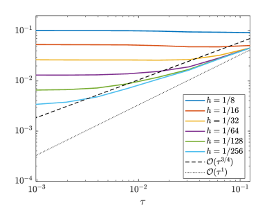
In Table 3 and Figure 9 we see, that convergence with respect to also for the approximation stochastic Barenblatt solution holds.
| 0.045434 | 0.022878 | 0.036722 | 0.040406 | 0.041319 | 0.041538 | |
| 0.06444 | 0.01176 | 0.021544 | 0.025007 | 0.025851 | 0.026057 | |
| 0.069643 | 0.012408 | 0.011412 | 0.014496 | 0.015296 | 0.01549 | |
| 0.074465 | 0.016884 | 0.0065525 | 0.0087332 | 0.0095565 | 0.0097648 | |
| 0.076666 | 0.020286 | 0.0057942 | 0.00491 | 0.0056214 | 0.0058322 | |
| 0.077362 | 0.02164 | 0.0063097 | 0.0029489 | 0.0031048 | 0.0032878 | |
| 0.077722 | 0.022367 | 0.0067772 | 0.0025539 | 0.0017667 | 0.0018573 | |
| 0.077983 | 0.022812 | 0.0070991 | 0.002603 | 0.0012162 | 0.0010803 |
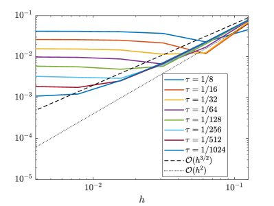
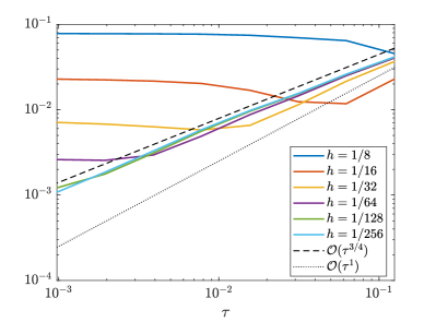
Figure 10 shows one sample path, the analytical support (for this path) is plotted in red and the support of the approximation in yellow. Finite speed of propagation hold a.s.
6.5. Numerical results for space-time noise
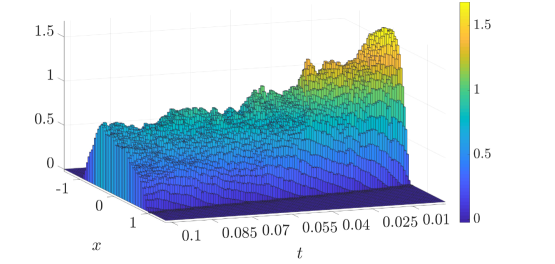
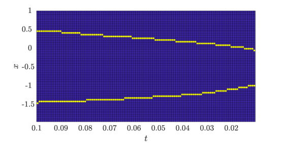
Next, we perform simulation of the stochastic porous media equation with space-time white noise on , , where no analytical solution is available. Given the the mesh size we take where where are the indicator functions of . We note that the -valued noise in an approximation of the multiplicative noise where is the space-time white noise, cf. [1].
In Figure 11 we display the numerical solution for one realization of the discrete space-time white noise with along with the corresponding support. We observe that the evolution of the support for the space-time white noise does not deviate significantly from the deterministic case. In particular the numerical approximation preserves the finite speed of propagation of the support, see Figure 12.
Acknowledgement
This work was supported by the Deutsche Forschungsgemeinschaft through SFB 1283 ”Taming uncertainty and profiting from randomness and low regularity in analysis, stochastics and their applications”.
References
- [1] E. J. Allen, S. J. Novosel, and Z. Zhang. Finite element and difference approximation of some linear stochastic partial differential equations. Stochastics Stochastics Rep., 64(1-2):117–142, 1998.
- [2] Viorel Barbu, Philippe Blanchard, Giuseppe Da Prato, and Michael Röckner. Self-organized criticality via stochastic partial differential equations. In Potential theory and stochastics in Albac, volume 11 of Theta Ser. Adv. Math., pages 11–19. Theta, Bucharest, 2009.
- [3] Viorel Barbu, Giuseppe da Prato, and Michael Röckner. Stochastic Porous Media Equations. Springer International Publishing, 2016.
- [4] Viorel Barbu and Michael Röckner. An operatorial approach to stochastic partial differential equations driven by linear multiplicative noise. J. Eur. Math. Soc. (JEMS), 17(7):1789–1815, 2015.
- [5] Viorel Barbu and Michael Röckner. Nonlinear Fokker–Planck equations driven by Gaussian linear multiplicative noise. Journal of Differential Equations, 265(10):4993–5030, November 2018.
- [6] Caroline Bauzet, Guy Vallet, and Petra Wittbold. A degenerate parabolic-hyperbolic Cauchy problem with a stochastic force. J. Hyperbolic Differ. Equ., 12(3):501–533, 2015.
- [7] Wolf-Jürgen Beyn, Benjamin Gess, Paul Lescot, and Michael Röckner. The Global Random Attractor for a Class of Stochastic Porous Media Equations. Comm. Partial Differential Equations, 36(3):446–469, 2011.
- [8] Garrett Birkhoff and Robert E. Lynch. Numerical solution of elliptic problems, volume 6 of SIAM Studies in Applied Mathematics. Society for Industrial and Applied Mathematics (SIAM), Philadelphia, PA, 1984.
- [9] K. Dareiotis, M. Gerencsér, and B. Gess. Entropy solutions for stochastic porous media equations. Journal of Differential Equations, 266(6):3732 – 3763, 2019.
- [10] Konstantinos Dareiotis, Máté Gerencsér, and Benjamin Gess. Porous media equations with multiplicative space-time white noise. arXiv preprint arXiv:2002.12924, 2020.
- [11] Konstantinos Dareiotis, Máté Gerencsér, and Benjamin Gess. Porous media equations with multiplicative space-time white noise. arXiv:2002.12924 [math], February 2020.
- [12] Konstantinos Dareiotis and Benjamin Gess. Supremum estimates for degenerate, quasilinear stochastic partial differential equations. arXiv:1712.06655, 2017.
- [13] Konstantinos Dareiotis and Benjamin Gess. Nonlinear diffusion equations with nonlinear gradient noise. Electron. J. Probab., 25:Paper No. 35, 43, 2020.
- [14] Konstantinos Dareiotis, Benjamin Gess, and Pavlos Tsatsoulis. Ergodicity of stochastic porous media equations. arXiv:1907.04605, 2019.
- [15] D. Dean. Langevin equation for the density of a system of interacting Langevin processes. Journal of Physics A: Mathematical and General, 29(24):L613, 1996.
- [16] Arnaud Debussche, Sylvain de Moor, and Martina Hofmanová. A Regularity Result for Quasilinear Stochastic Partial Differential Equations of Parabolic Type. SIAM J. Math. Anal., 47(2):1590–1614, 2015.
- [17] Arnaud Debussche, Martina Hofmanová, and Julien Vovelle. Degenerate parabolic stochastic partial differential equations: Quasilinear case. The Annals of Probability, 44(3):1916–1955, May 2016.
- [18] Felix Del Teso, Jørgen Endal, and Espen R Jakobsen. Robust numerical methods for nonlocal (and local) equations of porous medium type. part i: Theory. SIAM Journal on Numerical Analysis, 57(5):2266–2299, 2019.
- [19] Nicolas Dirr, Benjamin Fehrman, and Benjamin Gess. Conservative stochastic pde and fluctuations of the symmetric simple exclusion process. preprint, 2020.
- [20] Nicolas Dirr, Marios Stamatakis, and Johannes Zimmer. Entropic and gradient flow formulations for nonlinear diffusion. J. Math. Phys., 57(8):081505, 13, 2016.
- [21] A. Donev, T. G. Fai, and E. Vanden-Eijnden. A reversible mesoscopic model of diffusion in liquids: From giant fluctuations to Fick’s law. Journal of Statistical Mechanics: Theory and Experiment, 2014(4):P04004, April 2014.
- [22] Jérôme Droniou and Kim-Ngan Le. The gradient discretization method for slow and fast diffusion porous media equations. SIAM Journal on Numerical Analysis, 58(3):1965–1992, 2020.
- [23] Carsten Ebmeyer and WB Liu. Finite element approximation of the fast diffusion and the porous medium equations. SIAM journal on numerical analysis, 46(5):2393–2410, 2008.
- [24] Etienne Emmrich and David Šiška. Full discretization of the porous medium/fast diffusion equation based on its very weak formulation. Commun. Math. Sci., 10(4):1055–1080, 2012.
- [25] Etienne Emmrich and David Šiška. Nonlinear stochastic evolution equations of second order with damping. Stoch. Partial Differ. Equ. Anal. Comput., 5(1):81–112, 2017.
- [26] Benjamin Fehrman and Benjamin Gess. Path-by-path well-posedness of nonlinear diffusion equations with multiplicative noise. arXiv preprint arXiv:1807.04230, 2018.
- [27] Benjamin Fehrman and Benjamin Gess. Large deviations for conservative stochastic pde and non-equilibrium fluctuations. arXiv preprint arXiv:1910.11860, 2019.
- [28] Benjamin Fehrman and Benjamin Gess. Well-posedness of nonlinear diffusion equations with nonlinear, conservative noise. Archive for Rational Mechanics and Analysis, 233(1):249–322, 2019.
- [29] Julian Fischer and Günther Grün. Finite speed of propagation and waiting times for the stochastic porous medium equation: A unifying approach. SIAM Journal on Mathematical Analysis, 47(1):825–854, 2015.
- [30] Benjamin Gess. Strong solutions for stochastic partial differential equations of gradient type. J. Funct. Anal., 263(8):2355–2383, 2012.
- [31] Benjamin Gess. Finite speed of propagation for stochastic porous media equations. arXiv:1210.2415, pages 1–26, 2013.
- [32] Benjamin Gess. Random attractors for stochastic porous media equations perturbed by space-time linear multiplicative noise. Ann. Probab., 42(2):818–864, 2014.
- [33] Benjamin Gess. Finite time extinction for stochastic sign fast diffusion and self-organized criticality. Comm. Math. Phys., 335(1):309–344, 2015.
- [34] Benjamin Gess and Martina Hofmanová. Well-posedness and regularity for quasilinear degenerate parabolic-hyperbolic SPDE. The Annals of Probability, 46(5):2495–2544, 2018.
- [35] Benjamin Gess and Panagiotis E. Souganidis. Stochastic non-isotropic degenerate parabolic–hyperbolic equations. Stochastic Process. Appl., 127(9):2961–3004, 2017.
- [36] D. Gilbarg and N.S. Trudinger. Elliptic partial differential equations of second order. Classics in Mathematics. Springer-Verlag, Berlin, 2001. Reprint of the 1998 edition.
- [37] Benjamin Goldys, Michael Röckner, and Xicheng Zhang. Martingale solutions and Markov selections for stochastic partial differential equations. Stochastic Processes and their Applications, 119(5):1725–1764, May 2009.
- [38] H. Grillmeier and G. Grün. Nonnegativity preserving convergent schemes for stochastic porous-medium equations. Math. Comp., 88(317):1021–1059, 2019.
- [39] P. Grisvard. Elliptic problems in nonsmooth domains, volume 24 of Monographs and Studies in Mathematics. Pitman (Advanced Publishing Program), Boston, MA, 1985.
- [40] István Gyöngy. On stochastic squations with respect to semimartingales iii. Stochastics, 7(4):231–254, 1982.
- [41] I. n. Gyöngy and A. Millet. On discretization schemes for stochastic evolution equations. POTENTIAL ANALYSIS, 2005, 23, 2, 99, 2005.
- [42] Willi Jäger and Jozef Kačur. Solution of porous medium type systems by linear approximation schemes. Numerische Mathematik, 60(1):407–427, 1991.
- [43] Jong U. Kim. On the stochastic porous medium equation. J. Differential Equations, 220(1):163–194, 2006.
- [44] N. V. Krylov and B. L. Rozovskii. Stochastic evolution equations. Journal of Soviet Mathematics, 16(4):1233–1277, Jul 1981.
- [45] T. Lehmann, V. Konarovskyi, and M. von Renesse. Dean-Kawasaki Dynamics: Ill-posedness vs. Triviality. arXiv:1806.05018, June 2018.
- [46] J.-L. Lions. Quelques méthodes de résolution des problèmes aux limites non linéaires. Dunod; Gauthier-Villars, Paris, 1969.
- [47] Wei Liu and Michael Röckner. Stochastic Partial Differential Equations: An Introduction. Universitext. Springer, Cham, 2015.
- [48] E Magenes, RH Nochetto, and C Verdi. Energy error estimates for a linear scheme to approximate nonlinear parabolic problems. ESAIM: Mathematical Modelling and Numerical Analysis-Modélisation Mathématique et Analyse Numérique, 21(4):655–678, 1987.
- [49] S. Méléard and S. Roelly. Interacting measure branching processes. Some bounds for the support. Stochastics Stochastics Rep., 44(1-2):103–121, 1993.
- [50] J. Nečas. Les méthodes directes en théorie des équations elliptiques. Masson, 1967.
- [51] Hans Christian Öttinger. Beyond equilibrium thermodynamics. John Wiley & Sons, 2005.
- [52] Étienne Pardoux. Equations aux dérivées partielles stochastiques non linéaires monotones. PhD thesis, 1975.
- [53] Jiagang Ren, Michael Röckner, and Feng-Yu Wang. Stochastic generalized porous media and fast diffusion equations. Journal of Differential Equations, 238(1):118–152, 2007.
- [54] Luca Scarpa and Ulisse Stefanelli. Doubly nonlinear stochastic evolution equations. arXiv:1905.11294 [math], July 2019.
- [55] Roger Temam. Navier-Stokes equations, volume 2 of Studies in mathematics and its applications. North-Holland Publ., Amsterdam [u.a.], rev. ed. edition, 1979.
- [56] Michael Röckner (auth.) Viorel Barbu, Giuseppe Da Prato. Stochastic Porous Media Equations. Lecture Notes in Mathematics 2163. Springer International Publishing, 1 edition, 2016.
- [57] Juan Luis Vázquez. The porous medium equation. Oxford mathematical monographs. Clarendon Press, Oxford [u.a.], 2007.
- [58] Feng-Yu Wang. Exponential convergence of non-linear monotone SPDEs. Discrete and Continuous Dynamical Systems. Series A, 35(11):5239–5253, 2015.