Spatial interference between infectious hotspots: epidemic condensation and optimal windspeed

Spatial interference between infectious hotspots: epidemic condensation and optimal windspeed

Abstract

We discuss the effects of spatial interference between two infectious hotspots as a function of the mobility of individuals (wind speed) between the two and their relative degree of infectivity. As long as the upstream hotspot is less contagious than the downstream one, increasing the wind speed leads to a monotonic decrease of the infection peak in the downstream hotspot. Once the upstream hotspot becomes about between twice and five times more infectious than the downstream one, an optimal wind speed emerges, whereby a local minimum peak intensity is attained in the downstream hotspot, along with a local maximum beyond which the beneficial effect of the wind is restored. Since this non-monotonic trend is reminiscent of the equation of state of non-ideal fluids, we dub the above phenomena ”epidemic condensation”. When the relative infectivity of the upstream hotspot exceeds about a factor five, the beneficial effect of the wind above the optimal speed is completely lost: any wind speed above the optimal one leads to a higher infection peak. It is also found that spatial correlation between the two hotspots decay much more slowly than their inverse distance. It is hoped that the above findings may offer a qualitative clue for optimal confinement policies between different cities and urban agglomerates.

PACS Nos.: 87.23.Cc, 01.75.+m, 02.70.Bf

1 Introduction

In early 2020 the world has been taken by a very aggressive global pandemic, the covid-19, which spread around the entire planet at unprecedented speed in mankind history. As we speak, the pandemic, originated in Wuhan, China, allegedly in January 2020 has spread out over 100 countries, with over ten million contagion cases and over 500,000 casualties worldwide, as of end June 2020 [1], giving rise to the trade-off between strong confinement measures to stave off devastating effects on health systems [2, 3] and economic, social and psychological terms [4, 5, 6, 7].

A distinctive feature of the covid-19 pandemia is the heterogeneity of the viral infection in space; in many countries a large fraction of the overall infection counts originated from very specific hotspots, such as Lombardy in Italy and NYC in the USA. This strong inhomogeneity calls, among others, for a proper modelling of the mechanism by which the infection propagates in space and time [8].

In this paper we address this issue by isolating a toy-problem, namely the interaction between two infectious hotspots sitting at two separate locations in space. Special attention is paid to the spatial interference [9] between the two hotspots, in particular the way that the presence of the first affects the viral evolution in the second, depending on the mobility and infection rates in the two hotspots.

To this purpose, spatial mobility is described by a simple advection-diffusion SIR (ADSIR) model, in which diffusion encodes small-distance mobility (say walking), while advection stands for mid-range mobility (say train or car driving). Rather than being an exact model of these real-world mobility schemes – for which network models would certainly be a more accurate choice – diffusion and advection have the general purpose to realize two different mobility mechanisms with a different scaling in time and space. Even though human mobility proceeds by more complex mechanisms than AD, typically encoded by mobility networks [10, 11, 12, 13], the present ADSIR model exposes nonetheless a number of interesting qualitative features related the spatio-temporal coupling between the two infectious hotspots.

2 Mathematical formulation

We describe the covid-19 pandemic by means of a standard SIR model [14] – which is the starting point for numerous interesting models in epidemiology [15, 16, 17, 18, 11, 19, 7, 20] – coupled in space via an advection-diffusion mechanism:

$$\partial_{t}s=\nabla(-Us+D\nabla s)-\beta si$$ (1)

$$\partial_{t}i=\nabla(-Ui+D\nabla i)+\beta si-\gamma i$$ (2)

$$\partial_{t}r=\nabla(-Ur+D\nabla r)+\gamma i\$$ (3)

where $sir(x,y,t)$ is the population of Susceptible, Infected and Recovered individuals at position $x,y$ and time $t$, respectively. The coefficients $\beta,\gamma$ correspond to infection and recovery rate, respectively. In the above equations $U$ is the wind speed, which we take aligned with the x-axis without loss of generality and $D$ is the diffusivity. The total number of individuals of species $k=s,i,r$ at a given time $t$ is thus given by integral over the entire domain of the corresponding densities: $N_{k,h}(t)=\int_{H_{i}}n_{k}(x,y,t)dxdy,\;k=s,i,r,\;i=1,2$ where the integral runs over the hotspot regions HS1 and HS2.

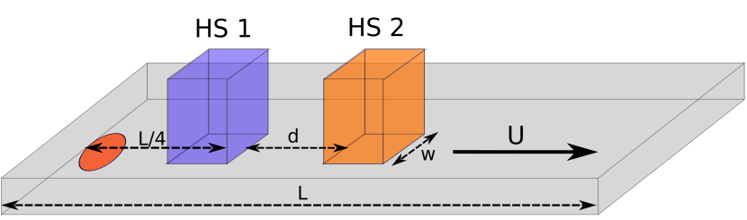
Figure 1: The simulation domain. Schematically shown is the simulation domain of length $L$. The boxes indicate the hotspots HS1 and HS2 with different contagion rate $\beta_{i}=f_{i}\times\beta_{0}$, where $\beta_{0}$ is the basic contagion rate in the normal domain. The hotspots at distance $d$ have width $w$ in both directions. The homogeneous wind $U$ is indicated by the black solid arrow and the red area indicates the small outbreak.

The speed $U$ will be compared to an important intrinsic reference velocity:

The infected population $i(t)$ grows in HS1 as $i(t)\approx A\cdot e^{(s(t)/N\cdot f_{1}\cdot\beta_{0}-\gamma)t}$. Whenever the wind exceeds a critical speed $U_{c}=w\cdot(s(t)/N\cdot f_{1}\cdot\beta-\gamma)$ mitigation of epidemics is expected, due to the removal of infected individuals from the hotspot.

For $U/U_{c}>1$, we expect the first hot-spot to become transparent and have little influence on the second one. This of course largely depends on the a priori unknown parameters $s(t)/N$ and the variable parameter $f_{1}$. For a reference, we take $f_{1}=f_{2}=50$ and $s(t)/N\approx 0.5$.

Hence, we define the reference speed $U_{r}=w\cdot(\frac{f_{2}\beta}{2}-\gamma)$.

The main independent (dimensionless) parameters are then defined as follows: The contagion rate is $\beta_{0}=0.2$ in the normal domain and $\beta_{i}=f_{i}\cdot\beta_{0}$ in the hotspots $i=1,2$. The recovery rate is homogeneous $\gamma=0.15$, such that the reproduction factor is $R_{i}=f_{i}\cdot\frac{\beta_{0}}{\gamma}>1$. We fix $f_{2}=50$ while $f_{1}$ ranges from $1$ to $500$, so that the relative infectivity ratio $f=f_{1}/f_{2}\in\left(0.02,10\right)$. The diffusion coefficient is $D=5$. The width of the hotspots is $w=10$ and their distance is $d=50$. The wind speed is measured in units of the reference speed, i.e. $u=U/U_{r}$. The grid spacing is $1\ \text{km}$ and time is measured in days, corresponding to a reference speed $U_{r}=50\ \text{km}/\text{day}$ and a diffusivity $D=5\ \text{km}^{2}/\text{day}$. These are plausible scales for human mobility.

We then study the solution of the ADSIR problem above as a function of the parameters $u$ and $f$.

In particular, we wish to assess under what conditions the presence of HS1 causes an increase of infections in HS2 in terms of both peak intensity and duration.

3 Simulation setup and results

We set up two hotspots HS1 and HS2 of width $w$ at position $x_{1}=L/4$ and $x_{2}=x_{1}+d+w$ respectively. The domain is a grid of size $64\times 1024$. We place a small Gaussian outbreak at $x=0$ and $y=W/2$ with a cutoff at $x=10$ in order to ensure that there are no initial infections in the hot-spots. The boundary conditions are chosen to be fully periodic. Fig. 1 shows the geometric set-up of the hot-spots in the domain.

In Fig. 2 we show the typical evolution of the infected species in a single hotspot. The starting time of the hot-spot is defined as the time $t_{s}$ at which the infected population reaches $i(t_{s})=0.002\cdot N$ and the end time $t_{e}$ at which the infected population has dropped to $i(t_{e})=0.05\cdot i_{max}$. The time difference $\Delta t=t_{e}-t_{s}$ can be defined as the duration of the epidemic in this region.

Figure 2: Time evolution of the SIR populations in a single hotspot. The baseline parameters are: $f_{1}=f_{2}=5$, $\beta=0.5$, $U=0$, $D=0.05$. The position of the hot-spot is at $x=L/4$. The red curve shows the infected population in the hotspot, the black x’s mark the start-up time, peak time and the decay time of the local epidemic, respectively.

In Figure 3, we report a typical spatial interference pattern between HS1 on HS2. The figure clearly shows that the infected population generated in HS1 reaches up to HS2 and increases the local infection rate, thereby increasing the peak and possibly the duration as well.

This is the typical scenario that HS2 policy makers endeavour to combat via lock-down measures.

Figure 3: Spatial distribution of the infected population. The y-integrated population with respect to the $x$-position. The hotspots are marked with vertical lines. The parameters are $f_{1}=f_{2}=50$, $\beta=0.2$, $\gamma=0.15$, and $u=0.28$, $d=50$, $w=10$, $D=0.05$. The snapshots are taken at the start-up time of both hotspots and the peak time of the second one. The development of a spatial interference between the two hotspots is clearly visible. The HS2 peak for the homogeneous case is $0.99\times 10=9.9$, against an observed one of about 12, showing a 20 percent increase due to spatial interference from HS2.

Peak and duration of the epidemics.–In Fig. 4, we summarize the effect of the wind and HS1 infectivity on the peak intensity of HS2.

Figure 4: Peak intensity in HS1 as a function of the wind speed at varying the infection rate in HS2 The simulation parameters are the same as in figure 3. We clearly observe the emergence of a non-monotonic wind speed regime in the range $1<f<5$, followed by a loss of any beneficial wind effect above $f\sim 5$.

We measure the dimensionless peak value $i_{max}/N$ in the second (downstream) hotspot as a function of $u$ and $f$, where $N$ is the total number of individuals in the hotspot and $i_{max}$ is the peak value of the infected population.

A few comments are in order.

First, we see that the peak intensity is a fast decreasing function of the wind speed for all HS1 infection ratios well below the HS2 values. This is expected, since the infected in HS2 get replaced by less infected from HS1.

However, upon increasing $f_{1}$ in the vicinity and then above $f_{2}$, a shoulder appears at intermediate wind speeds, indicating that a highly contagious mobile population from HS1 is capable of spoiling the beneficial effect of the wind. This is also a plausible result, since the infected removed by the wind in HS2 are quickly replaced by even more infected transmitted by HS1. This is the typical scenario dreaded by southern Italy towards the ”stampede” from northern regions in the early stage of the Italian epidemics.

Our simple model shows that such fears were indeed justified, an infectivity ratio $f=2$ is already capable of producing a secondary peak in the curve and raising $f$ only makes the situation worst, with the emergence of a whole range of wind speeds in which the peak intensity grows instead of decaying, almost reaching up to the value of the windless case.

Since this strongly reminds of the unstable region of a non-ideal equation of state, in which pressure goes down upon increasing density (condensation), we dub this effect ”epidemic condensation”.

This is the main result of this paper, as it highlights the existence of an optimal wind speed $u_{min}\sim 0.5$ which minimises the HS2 peak, and a second, higher, characteristic speed $u_{max}$, beyond which the beneficial effects of the wind are restored. By further increasing the relative infectivity of HS1, between five and ten, no decay of the peak intensity at increasing wind speed above $u_{min}$ is observed anymore in the simulated window of the wind speed $u$, indicating that the presence of HS1 completely cancels any benefit of the wind speed above the optimal value $u_{min}$. However, for a very large wind speed $u\to\infty$ we expect again a decrease of the infected ratio, since for infinite wind speed the hot-spots become transparent again, and infectivity will have no impact.

In Fig. 5 we report the duration of the epidemics as a function of $u$ and $f$. A major peak is observed at low-wind, corresponding to the fact that the infected are convected away at very low rates. As expected, high infectivity goes with high peaks and short durations, the dreaded scenario for intensive care departments.

As the wind speed increases, the local infected are efficiently removed and the epidemic duration shortens. However, starting from comparatively low infectivity ratios, $f=0.2$, further satellite peaks appear, indicating the existence of a sequence of wind speeds such that the duration grows back, if only mildly. This is again interpreted as a spatial interference effect, although we must caution that such measurement is very sensitive to small changes of the duration threshold, hence should be taken with great caution.

Figure 5: Duration of the epidemic in HS2. The curve shows a peak at very low wind speeds $u\sim 0.01$, followed by a sequence of secondary peaks at higher speeds, all well below $u_{min}$. By and large, wind speeds above $u=0.1$ are consistently beneficial in shortening the epidemic duration.

4 Qualitative scenario and discussion

The ADSIR model presented in this paper focusses on the effects of spatial coupling, advection and diffusion, on epidemic growth as dictated by local infection rates. It is well known that in the presence of random heterogeneities, such coupling can lead to highly nontrivial behaviour, such as the formation of striated infection highways [21].

Here we take a simpler model problem, namely the effect of a primary hotspot (HS1) on the epidemic growth on a secondary hotspot (HS2) downstream HS1. In particular, we focus on the effect of a uniform ”wind” at speed $u$, mimicking a uniform human mobility across the two hotspots.

In the absence of any wind, $u=0$, and discounting diffusion, the two hotspots evolve independently based on their corresponding infection rates.

As soon as the wind is switched on, a beneficial effect is expected for both HSs because the wind sweeps infected individuals away into the ”country side”, where the chance to infect is much lower and healing can proceed nearly undisturbed. This is certainly true as soon as the wind speed exceeds the infection speed, namely the size of the hotspot divided by the typical infection timescale (reference speed), because, under such conditions, the wind blows susceptible individuals away before they have time to get significantly infected.

So, the baseline expectation is that ”wind is good”, as it gives no time for infection to develop substantially. This is true for HS1, but not necessarily for HS2, which is exposed to the incoming flux of infected individuals from HS1.

The quantitative question is whether, from the HS2 perspective, there exists an optimal wind speed which corresponds to a local minimum of the infection peak .

In the following, we shall present evidence that the answer is in the affirmative. In particular, it is shown that as soon as HS1 is more infectious than HS2, the peak intensity in HS2 develops a much slower decay with the wind speed, and when HS1 is significantly more infectious than HS2, the HS2 peak increases at increasing wind speed, before it starts to decay again in the strong wind regime. In other words, the HS2 peak develops a non-monotonic dependence on the wind speed, with a local minimum, $u_{min}$ at about half the reference speed and a local maximum $u_{max}$ about twice as large.

Such non-monotonic dependence bears an intriguing resemblance to a non-ideal equation of state, with the unstable branch in the wind speed region $u_{min}\leq u\leq u_{max}$. Because of this close resemblance to equation of state of non-ideal gas, and most notably to the unstable region where a density increase leads to a pressure decrease (condensation), we dub this effect epidemic condensation.

We also monitor the duration of the epidemics as a function of the wind speed and infection rates. Note that while the peak intensity is the prime concern for health capacity issues, the duration bears directly on the mid-long term policies towards social and economic impact (many countries insisted on ”curve flattening” policies).

Again, we find that wind increase above a very low threshold is generally beneficial, although at increasing HS2 infectivity, the duration increases and shows repeated small-amplitude ”sawtooth” oscillations. Such oscillations are yet another signature of spatial coupling, although their specific nature remains to be fully ascertained.

5 Effect of the hotspot distance and the diffusivity

We also inspected the effect of the hotspot distance on epidemic condensation. To this purpose, we ran a series of simulations at different wind speeds and distances in the range $50\leq d\leq 200$, keeping a fixed value $f=4$.

As expected, the local maximum observed in the condensation decreases with the distance and, less expectedly, so does the local minimum.

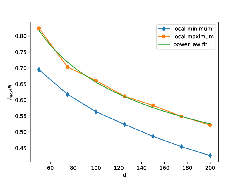
Figure 6: The local minimum and maximum of the condensation curve. The infectivity ratio is set to be $f=4$, all other parameters are chosen as in Fig. 4. Shown are the local minimum and maximum of the curve of the infected ratio in HS 2. The power-law fit is performed with a small exponent, $d^{-0.32}$, hence the correlation effects decay slower than the distance.

Fig. 6 shows that both quantities decay according to an inverse power law $d^{-\alpha}$, with $\alpha\sim 1/3$, indicating that the correlation between the two hotspots decays much more slowly than their inverse distance. To assess the effect of the diffusivity, we computed the condensation curve – similar to Fig. 4 with fixed $f=4$, for different values of the diffusion constants $D$.

Figure 7: Effect of diffusion. We change the diffusivity and inspect its effect on the condensation curve for an intermediate high infectivity ratio $f=4$. For small $D$, we observe no qualitative change of the curve. $D=5\,km^{2}/day$ is the value we used throughout the rest of this paper. When the Fischer speed $U_{f}=\sqrt{Df_{1}\beta_{0}}$ approaches the reference wind speed $U_{r}$, we expect additional interference effects which may lead a revival of infectivity in HS2. A detailed study of these phenomena is left to a future study.

In Fig. 7 we observe a quantitative effect of the diffusion parameter on the condensation curve, due to the fact that diffusion smears out sharp spatial changes in population number, such as those observed at the hot-spot boundaries.

Hence, the effect of increasing the diffusivity $D$ is similar to lowering the infectivity ratio $f$, as long as the diffusivity remains sufficiently small enough, meaning by this that the Fisher speed $U_{f}=\sqrt{Df_{1}\beta_{0}}$ remains well below the reference wind speed. In the simulations carried out here, $U_{f}$ is always significantly smaller than $U_{r}$, hence these effects do not play any role. Whenever the condition $U_{f}\ll U_{r}$ is violated, non trivial interference effects are expected, which may eventually lead to a revival of infectivity in the second hotspot. A detailed analysis of these effects warrants a separate study on its own, hence it is deferred to future investigations.

6 Conclusions

Summarizing, we have evidenced a non-monotonic relation between the wind speed and the peak intensity on the downstream hotspot as a function of the infectivity ratio with respect to the upstream one. Despite its drastic simplification of the mechanism of human mobility, it is hoped that the non-monotonic ”constitutive relation” revealed by the present ADSIR model, as shown in Figures 4 and 5, may offer useful qualitative clues on the effects of spatial interference between infected hotspots.

References

- [1] J. H. University, Covid-19 dashboard worldwide 2020.
- [2] B. Armocida, B. Formenti, S. Ussai, F. Palestra and E. Missoni, The Lancet Public Health 5, p. e253 (2020).
- [3] H. Legido-Quigley, J. T. Mateos-García, V. R. Campos, M. Gea-Sánchez, C. Muntaner and M. McKee, The Lancet Public Health 5, e251 (2020).
- [4] Q. Chen, M. Liang, Y. Li, J. Guo et al., The Lancet Psychiatry 7, e15 (2020).
- [5] L. Duan and G. Zhu, The Lancet Psychiatry 7, 300 (2020).
- [6] M. Nicola, Z. Alsafi, C. Sohrabi, A. Kerwan et al., International Journal of Surgery 78, 185 (2020).
- [7] A. A. Toda, (2020) arXiv:2003.11221.
- [8] A. L. Lloyd and R. M. May, Journal of Theoretical Biology 179, 1 (1996).
- [9] K. Dietz, Journal of Mathematical Biology 8, 291 (1979).
- [10] F. Ball, D. Sirl and P. Trapman, Mathematical Biosciences 224, 53 (2010).
- [11] J. C. Lang, H. De Sterck, J. L. Kaiser and J. C. Miller, Journal of Complex Networks 6, 948 (2018).
- [12] M. U. Kraemer, C. H. Yang, B. Gutierrez, C. H. Wu et al., Science 368, 493 (2020).
- [13] M. Chinazzi, J. T. Davis, M. Ajelli, C. Gioannini et al., Science 368, 395 (2020).
- [14] W. O. Kermack and A. G. McKendrick, Proceedings of the Royal Society A: Mathematical, Physical and Engineering Sciences 115, 700 (1927).
- [15] S. Kaushal, A. S. Rajput, S. Bhattacharya, M. Vidyasagar et al., (2020) arXiv:2006.00045 .
- [16] E. Kaxiras, G. Neofotistos and E. Angelaki, Chaos, Solitons and Fractals 138, 1 (2020).
- [17] S. Pathak, A. Maiti and G. P. Samanta, Nonlinear Analysis: Modelling and Control 15, 71 (2010).
- [18] C. Ji, D. Jiang and N. Shi, Physica A: Statistical Mechanics and its Applications 390, 1747 (2011).
- [19] W. C. Roda, M. B. Varughese, D. Han and M. Y. Li, Infectious Disease Modelling 5, 271 (2020).
- [20] G. C. Calafiore, C. Novara and C. Possieri, (2020) arxiv:2003.14391.
- [21] T. Chotibut, D. R. Nelson and S. Succi, Physica A: Statistical Mechanics and its Applications 465, 500 (2017).