Converting Lattices into Networks: The Heisenberg Model and Its Generalizations with Long-Range Interactions

Abstract

In this paper, we convert the lattice configurations into networks with different modes of links and consider models on networks with arbitrary numbers of interacting particle-pairs. We solve the Heisenberg model by revealing the relation between the Casimir operator of the unitary group and the conjugacy-class operator of the permutation group. We generalize the Heisenberg model by this relation and give a series of exactly solvable models. Moreover, by numerically calculating the eigenvalue of Heisenberg models and random walks on network with different numbers of links, we show that a system on lattice configurations with interactions between more particle-pairs have higher degeneracy of eigenstates. The highest degeneracy of eigenstates of a lattice model is discussed.

1 Introduction

Lattice models are important because they can be not only treated theoretically, for example the Heisenberg models can be solved exactly at lower dimensions [1, 2, 3], but also implemented experimentally, such as constraining ultracold atoms in optical lattices [4, 5]. Among many lattice models, the Heisenberg model which describes the magnetism of a system [1, 2, 3] is of significance. To solve the Heisenberg model, methods such as the Bethe Ansatz and the Jordan Wigner transformations are proposed [1, 6]. The solution of the Heisenberg model at different dimensions [7, 8, 9] or under certain boundary conditions [10, 11, 12] is discussed.

In this paper, we solve the Heisenberg model by using a group theory method. In the group theory method suggested in the present paper, we reveal the relation between the Casimir operator of the unitary group and the conjugacy-class operator of the permutation group. We propose a generalization of the Heisenberg model which can be solved exactly.

(1) Converting lattice configurations into networks. We consider a model on lattice configurations with arbitrary numbers of interacting particle-pairs by converting the lattice configuration into networks. Usually, lattice models with certain number of neighbours or interacting particle-pairs are taken into account. For example, $3$, $4$, $6$, etc. It is because only countable lattice configurations exist under the constraint of symmetries [13, 14]. For example, there are $17$ kinds of two-dimensional lattice models and there are $230$ kinds of three-dimensional lattice models. In this paper, we map the lattice configuration to networks with different modes of links, as shown in Fig. (1). We show that the number of nearest particles is characterized by the number of links in the network. The advantage of doing this is that we are free to consider a systems with arbitrary number of interacting particle-pairs which in lattice configurations is restricted by symmetries. By studying the relation between degeneracy of eigenstates and the number of the interacting particle-pairs, we show that models on lattice configuration with more interacting particle-pairs have higher degeneracy of eigenstates. Thus, lattice models with interactions between all particle-pairs should have a highest degeneracy of eigenstates.

(2) The Long-Range Interactions. The lattice model with long-range interaction between inter-particles is considered. Usually, short-range interactions are considered in lattice models, as a result, only the interaction between nearest, second nearest, third nearest, etc, particle-pairs need to be considered. However, if long-range interactions, such as the inverse square potential and the harmonic oscillator potential, exist, interactions between more particle-pairs need to be considered. For example, one-dimensional models with long-range interactions is considered in [15]. Ising models on the hypercube lattices with long-range interaction is considered in [16]. In this paper, the model on lattice configuration with interaction between all particle-pairs is with long-range interactions.

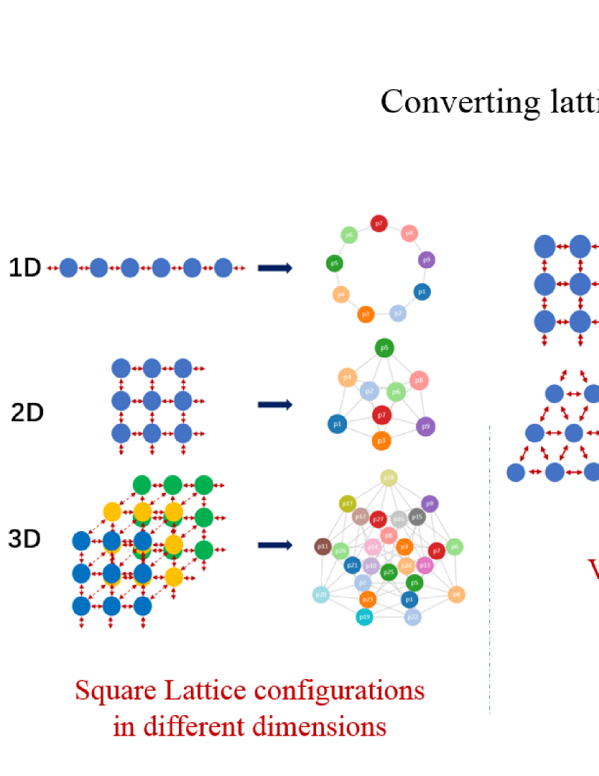
Figure 1: Converting lattice configurations into networks. By holes or impurities, we mean that they can not interact with other particles. The periodic boundary condition is applied.

This paper is organized as follows: In Sec. 2, we solve the Heisenberg model on lattice configurations with interactions between all particle-pairs by revealing the relation between the Casimir operator of the unitary group and the conjugate class operator of the permutation group. In Sec. 3, we give a series of exactly solvable models by generalizing the Heisenberg model from this relation. In Sec. 4, we investigate the relation between degeneracy of eigenstates and the number of links in a network by numerically calculating the eigenvalues of Heisenberg models and random walks on a network. We discuss the highest degeneracy of eigenstates for a interacting many-body system. Conclusions and discussions are given in Sec. 5.

2 The Heisenberg model on lattice configurations with interactions between all particle-pairs

In this section, we consider the Heisenberg model on lattice configurations with interactions between all particle-pairs.

A special lattice configuration: lattice configurations with interactions between all particle-pairs. As shown in Fig. (1), for various kinds of lattice configurations the difference varies in the mode of links between particles other than the position of particles. The network with links between all particle-pairs considers the largest number of particle-pairs interactions, as shown in Fig. (2). In the following, we will make no distinguish between lattice configurations and networks.

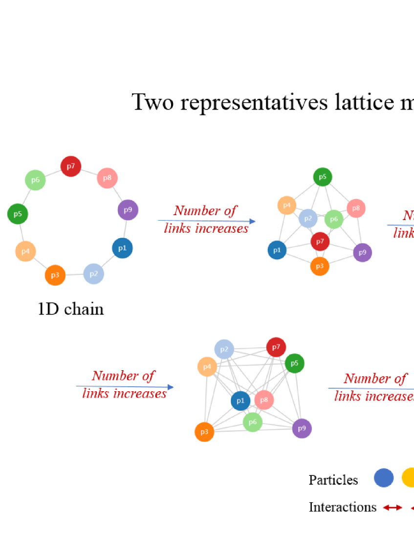
Figure 2: The lattice configuration with interactions between all particle-pairs and the one-dimensional lattice configuration are two special lattice configurations: one considers the largest number of links and the other considers the smallest number of links.

The Hamiltionian of the Heisenberg model with interactions between all particle-pairs. Here, we show that the Hamiltonian of the Heisenberg model on the lattice configuration with interactions between all particle-pairs can be expressed in terms of the Casimir operators of $U\left(2\right)$ group. We give the eigenvalue spectrum of the system. For the sake of clarity, in this section, we directly give the result. The detail of calculations will be given in Sec. 3. For the Heisenberg model on lattice configurations with interactions between all particle-pairs, the Hamiltonian reads

$$H=\sum_{\left(i,j\right)}\frac{1}{2}\mathbf{S}_{i}\cdot\mathbf{S}_{j},$$ (2.1)

where $\mathbf{S}_{i}$ is the spin of $ith$ particle and $\sum_{\left(i,j\right)}$ runs all pairs of particles. With simple transformations, the Hamiltonian, Eq. (2.1), can be written as

$$H=\sum_{\left(i,j\right)}\tau_{ij}-\sum_{\left(i,j\right)}\mathbf{e}\cdot\mathbf{e},$$ (2.2)

where $\tau_{ij}$ if the action of permutation of particles with index $i$ and $j$. and $\mathbf{e}$ is the identity matrix. By using the relation between the Casimir operator of unitary group and the conjugacy-class operator of permutation group, which, for the sake of clarity, will be provided in Sec. 3.1, one can rewrite Eq. (2.2) in the form

$$H\mathbf{=}P_{\left(1^{N-2},2\right)}=\frac{1}{2}C_{2}-C_{1},$$ (2.3)

where $C_{2}$ and $C_{1}$ are the Casimir operator of the unitary group $U\left(2\right)$ with order $2$ and $1$, respectively. $P_{\left(1^{N-2},2\right)}$ is the conjugacy-class operator of the symmetrical group.

The eigenvalue spectrum. The Hamiltionain, Eq. (2.3), shows that the eigenvalue of the Hamiltionain can be obtained once the eigenvalues of the Casimir operator of the unitary group $U\left(2\right)$ are given. For a system consisting of $N$ particles, the irreducible representation of $U\left(2\right)$ is indexed by a single parameter $s$, an integer ranges from $0$ to the largest integer smaller than $N/2$ [17]. By using the eigenvalue of the Casimir operator of $U\left(2\right)$ in a given representation [17], we give the eigenvalue of the Hamiltionain, Eq. (2.3):

$$E_{s}=2s^{2}-2Ns-2s+\frac{1}{2}N^{2}-\frac{1}{2}N.$$ (2.4)

The degeneracy of energy $E_{s}$ is $\omega_{s}$

$$\omega_{s}=\frac{\left(1+N-2s\right)^{2}N!}{\left(1+N-s\right)!s!}.$$ (2.5)

3 A generalization of the Heisenberg model

In this section, we construct a series of exactly solvable models. These models are the generalization of the Heisenberg model using the relation between the Casimir operator of the unitary group and the conjugacy-class operator of permutation group. This method provides us an easier way to give the spectrum of the many-body spin system. As shown in Sec. 2, setting $m=2$ recovers the Heisenberg model. For the generalized model, bosonic and fermionic realizations are discussed below.

3.1 The Casimir operator of the unitary group and the conjugacy-class operator of the permutation group: a brief review

The Casimir operator of the unitary group $U\left(m\right)$. The unitary group $U\left(m\right)$ has $m$ linear-independent Casimir operators. The Casimir operator of order $l$, denoted by $C_{l}$, is [17]

$$C_{l}=\sum_{k_{1},k_{2},...,k_{l-1}}E_{k_{1}k_{2}}E_{k_{2}k_{3}}...E_{k_{l-2}k_{l-1}}E_{k_{l-1}k1}$$ (3.1)

where $E_{kl}$ is the generator of $U\left(m\right)$ .

The irreducible representation of $U\left(m\right)$ is indexed by $m$ nonnegative integers denoted by $\left(a\right)=\left(a_{1},a_{2},\ldots,a_{m}\right)$ with $a_{1}\geqslant a_{2}\geqslant...\geqslant a_{m}\geqslant 0$ [17]. The eigenvalue of the Casimir operator $C_{l}$, denoted by $\left\langle C_{1}\right\rangle$, under the representation indexed by $\left(a\right)$ is [17]

$$\left\langle C_{1}\right\rangle =S_{1}$$ (3.2)

$$\left\langle C_{2}\right\rangle =S_{2}-\left(m-1\right)S_{1}$$ (3.3)

$$\left\langle C_{3}\right\rangle =S_{3}-\left(m-\frac{3}{2}\right)S_{2}-\frac{1}{2}S_{1}^{2}-\left(m-1\right)S_{1}$$ (3.4)

$$\ldots,$$ (3.5)

where

$$S_{k}=\sum_{i=1}^{m}\left[\left(a_{i}+m-i\right)^{k}-\left(m-i\right)^{k}\right].$$ (3.6)

The conjugacy-class operator of the permutation group $S_{N}$. The sum of all the group elements which belong to the same conjugacy class gives a conjugacy-class operator [18]. The conjugacy-class operator commutes with all the group elements [18]. For the permutation group of order $N$, each integer partition of $N$ (a representation of $N$ in terms of the sum of other integers) gives a corresponding conjugacy-class operator [18]. In this paper, we focus on the conjugacy-class operator corresponding to the integer partition $\left(\lambda\right)=\left(1^{N-2},2\right)$ with superscript $N-2$ standing for $1$ appearing $N-2$ times. By definition, the conjugacy-class operator reads

$$P_{\left(1^{N-2},2\right)}=\sum_{1=i<j}^{N}\tau_{ij},$$ (3.7)

where $\tau_{ij}$ is the exchange of the $ith$ and the $jth$ particle.

3.2 A relation between the Casimir operator of the unitary group and the conjugate class operator of the permutation group

In this section, we introduce a relation between the Casimir operator of the unitary group and the conjugacy-class operator of the permutation group. This relation makes it easier to calculate the eigenvalue spectrum of the Heisenberg model .

The relation between $C_{l}$ and $P_{\left(1^{N-2},2\right)}$. The conjugacy-class operator $P_{\left(1^{N-2},2\right)}$ of the permutation group satisfies

$$P_{\left(1^{N-1},2\right)}=\frac{1}{2}C_{2}-\frac{m}{2}C_{1},$$ (3.8)

where $C_{1}$ and $C_{2}$ are the Casimir operators of order $1$ and $2$ of the unitary group.

Proof. Let $a_{k}^{\dagger i}$ with superscript ranging from $1$ to $N$ and subscript ranging from $1$ to $m$ represents creating the $ith$ particle in the state $k$. $a_{k}^{i}$ is the annihilation operator, which represents the conjugate of $a_{l}^{\dagger j}$. The commutation relation between $a_{k}^{\dagger i}$ and $a_{l}^{j}$ is

$$\left[a_{k}^{i},a_{l}^{\dagger j}\right] =\delta_{ij}\delta_{kl},$$ (3.9)

$$\left[a_{k}^{i},a_{l}^{j}\right] =\left[a_{k}^{\dagger i},a_{l}^{\dagger j}\right]=0.$$ (3.10)

The generator $\tau_{ij}$ of $S_{N}$ can be expressed in terms of $a_{l}^{j}$ and $a_{l}^{\dagger j}$ [18]:

$$\tau_{ij}=\sum_{k,l=1}^{m}a_{k}^{\dagger i}a_{l}^{\dagger j}a_{l}^{i}a_{k}^{j}.$$ (3.11)

The generator of $U\left(m\right)$ can also be expressed as:

$$E_{kl}=\sum_{i=1}^{N}a_{k}^{\dagger i}a_{l}^{i}.$$ (3.12)

Substituting Eq. (3.11) with $\tau_{ij}$ into Eq. (3.7) gives the conjugacy-class operator:

$$P_{\left(1^{N-2},2\right)}=\sum_{1=i<j}^{N}\sum_{k,l=1}^{m}a_{k}^{\dagger i}a_{l}^{\dagger j}a_{l}^{i}a_{k}^{j}.$$ (3.13)

Substituting Eq. (3.12) with $E_{kl}$ into Eq. (3.1) gives the Casimir operator:

$$C_{2} =\sum_{i,j}^{N}\sum_{k,l=1}^{m}a_{k}^{\dagger i}a_{l}^{\dagger j}a_{l}^{i}a_{k}^{j}C,$$ (3.14)

$$C_{1} =\sum_{i=1}^{N}\sum_{l=1}^{m}a_{l}^{\dagger i}a_{l}^{i}.$$ (3.15)

So the operator relation between $P_{\left(1^{N-2},2\right)}$ and $C_{l}$ becomes

$$\frac{1}{2}C_{2}-\frac{m}{2}C_{1}=P_{\left(1^{N-1},2\right)}+\frac{1}{2}\sum_{k,l=1}^{m}\sum_{i=1}^{N}a_{k}^{\dagger i}a_{l}^{\dagger i}a_{l}^{i}a_{k}^{i},$$ (3.16)

where Eq. (3.13) is used. The last term of Eq. (3.16) can be written as

$$\sum_{k,l=1}^{m}\sum_{i=1}^{N}a_{k}^{\dagger i}a_{l}^{\dagger i}a_{l}^{i}a_{k}^{i}=\sum_{i=1}^{N}\left[\sum_{l=1}^{m}n_{l}^{i}-\left(\sum_{l=1}^{m}n_{l}^{i}\right)\left(\sum_{l=1}^{m}n_{l}^{i}\right)\right],$$ (3.17)

by introducing $N_{i}\equiv\sum_{l=1}^{m}n_{l}^{i}$ with $n_{l}^{i}$ equaling to $a_{l}^{\dagger i}a_{l}^{i}$. $N_{i}$ represents the number of $ith$ particle, that is $1$. Therefore, the equation

$$\sum_{k,l=1}^{m}\sum_{i=1}^{N}a_{k}^{\dagger i}a_{l}^{\dagger i}a_{l}^{i}a_{k}^{i}=0$$ (3.18)

holds. Eq. (3.8) is proved.   

3.3 The generalization

In this section, by using the relation between the Casimir operator of the unitary group and the conjugacy-class operator of the permutation group, Eq. (3.8), we construct a series of exactly solvable models which are generalizations of the Heisenberg model. They are models on lattice configurations with interactions between all particle-pairs.

The Hamiltionian. The Hamiltonian of the model is

$$H=\frac{1}{2}C_{2}-\frac{m}{2}C_{1}$$ (3.19)

with $C_{1}$ and $C_{2}$ the Casimir operators of $U\left(m\right)$. Such systems consist of $N$ $m$-states particles. The Hamiltonian $H$ in Eq. (3.19) exchanges all particle-pairs in the system, that is

$$H\left(v_{1}\otimes v_{2}\otimes v_{3}\otimes...\otimes v_{N}\right)=v_{2}\otimes v_{1}\otimes v_{3}\otimes...\otimes v_{N}+v_{1}\otimes v_{3}\otimes v_{2}\otimes...\otimes v_{N}+\ldots.$$ (3.20)

Therefore, the generalized models are on lattice configurations with interactions between all particle-pairs.

The eigenvalue spectrum. Eq. (3.19) shows that, the eigenvalue of the Hamiltionain can be obtained provided the eigenvalues of the Casimir operator of the unitary group $U\left(m\right)$ are given. The eigenvalues of the Casimir operator of the unitary group $U\left(m\right)$ are indexed by $m$ nonnegative integers denoted by $\left(a\right)=\left(a_{1},a_{2},...,a_{m}\right)$ with $a_{1}\geqslant a_{2}\geqslant...\geqslant a_{m}\geqslant 0$ [17]. The summation of $\left(a\right)$ is $N$, i.e., $\sum_{i=1}^{m}a_{i}=N$. By using the eigenvalue of the Casimir operator given in Eqs. (3.2)-(3.3), we give the eigenvalue of the Hamiltionain, Eq. (3.19),

$$E_{\left(a\right)}=\frac{1}{2}\sum_{i=1}^{m}a_{i}^{2}-\sum_{i=1}^{m}a_{i}i+\frac{1}{2}N.$$ (3.21)

The degeneracy of $E_{\left(a\right)}$ is

$$\omega_{\left(a\right)}=N!{\displaystyle\prod\limits_{i<j}^{m}}\frac{\left(a_{i}-a_{j}-i+j\right)}{\left(j-i\right)}\frac{{\displaystyle\prod\limits_{i^{\prime}<j^{\prime}}^{l}}\left(a_{i^{\prime}}-a_{j^{\prime}}-i^{\prime}+j^{\prime}\right)}{{\displaystyle\prod\limits_{i^{\prime\prime}=1}^{l}}\left(l+a_{i^{\prime\prime}}-i^{\prime\prime}\right)!},$$ (3.22)

where $l$ is the number of positive integers in $\left(a\right)$.

A bosonic realization: an example. By expressing the generators of $U\left(m\right)$ in terms of the Boson operators $a_{i}^{\dagger}$ and $a_{j}$ with commutation relation

$$\left[a_{i},a_{j}^{\dagger}\right] =\delta_{ij},$$ (3.23)

$$\left[a_{k},a_{j}\right] =\left[a_{k}^{\dagger},a_{l}^{\dagger}\right]=0,$$ (3.24)

the Hamiltonian of the system, Eq. (3.19), can be written as

$$H=\frac{1}{2}\sum_{i,j=1}^{m}a_{i}^{\dagger}a_{j}a_{j}^{\dagger}a_{i}-\frac{m}{2}\sum_{i=1}^{m}a_{i}^{\dagger}a_{I}.$$ (3.25)

By using Eqs. (3.21) and (3.22) with $a_{1}=N$ and $a_{i}=0$ for $i>1$, we can obtain the eigenvalue and degeneracy of the system:

$$E_{n}=\frac{1}{2}n^{2}-\frac{1}{2}n,$$ (3.26)

$$\omega_{n}=\frac{n!{\displaystyle\prod\limits_{l=1}^{m-1}}\left(l+n\right)^{2}}{\left(m-1\right)!\left(n+m-1\right)!}.$$ (3.27)

A fermionic realization: an example. By expressing the generators of $U\left(m\right)$ in terms of the Fermi operators $b_{i}^{\dagger}$ and $b_{j}$ with commutation relation

$$\left\{b_{i},b_{j}^{\dagger}\right\} =\delta_{ij},$$ (3.28)

$$\left\{b_{i}^{\dagger},b_{j}^{\dagger}\right\} =\left\{b_{i},b_{j}\right\}=0,$$ (3.29)

the Hamiltonian of the system, Eq. (3.19), can be written as

$$H=\frac{1}{2}\sum_{i,j=1}^{m}b_{i}^{\dagger}b_{j}b_{j}^{\dagger}b_{i}-\frac{m}{2}\sum_{i=1}^{m}b_{i}^{\dagger}b_{i}$$ (3.30)

The eigenvalue and degeneracy, by using Eqs. (3.21) and (3.22) with $a_{i}=a_{j}=1$, are expressed as

$$E_{n}=-\frac{n^{2}}{2}+\frac{1}{2}n,$$ (3.31)

$$\omega_{n}=\frac{m!}{\left(m-n\right)!n!}.$$ (3.32)

Notice that, in Bose and Fermi cases, such system have no-fixed particle numbers.

4 The degeneracy of eigenstates of a lattice model

In a lattice model, usually the nearest number of particle is a finite numbers, such as 3, 4, 6, and so on, due to the constraint of symmetries. Therefore, one only considers interactions between nearest particle-pairs, second nearest particle-pairs, and so on. In this paper, by converting the lattice configurations into networks, we can consider models with arbitrary number of interacting particle-pairs. That is, we can consider models on networks with different modes of links. In this section, we investigate the relationship between degeneracy of eigenstates and the number of links in networks, by numerically calculating the Heisenberg models and random walks on network with different number of links. It shows that models on networks with more links tend to have higher degeneracy of eigenstates.

4.1 Heisenberg models and random walks on networks with different numbers of links

Various models can be considered on a network or lattice configurations. In this section, we consider Heisenberg models and random walks on networks with different modes of links.

Heisenberg models. In this section, we study the isotropic Heisenberg models with Hamiltionain $H$ reads

$$H=\sum\frac{1}{2}\mathbf{S}_{i}\cdot\mathbf{S}_{j},$$ (4.1)

where $\mathbf{S}_{i}$ is the spin of $ith$ particle and $\sum$ represents summation over particle-pairs with links. The eigenvalue spectrum of Heisenberg models, Eq. (4.1), in different dimensions and on networks with random links are given in Figs (3) and (4).

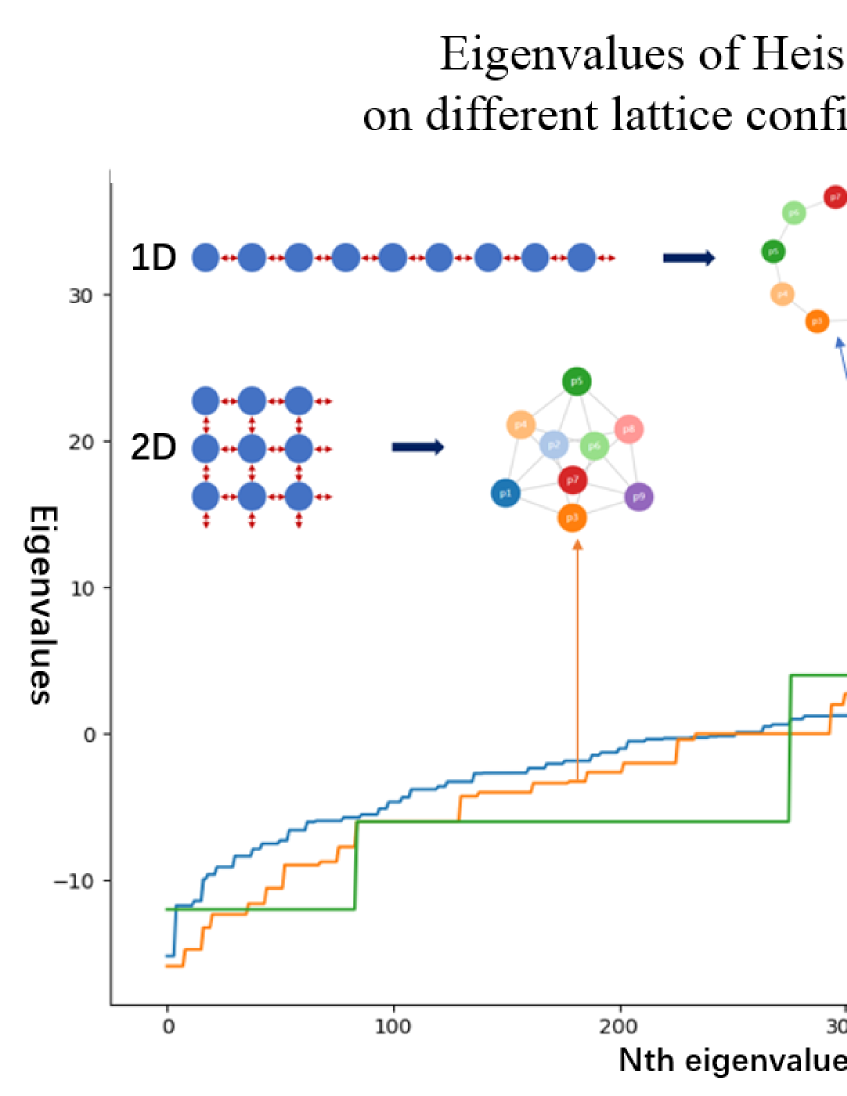
Figure 3: The eigenvalue of Heisenberg model consisting of $9$ particles in different dimensions. as shown, $1$D represents a line configuration, $2$D represents a plain configuration.

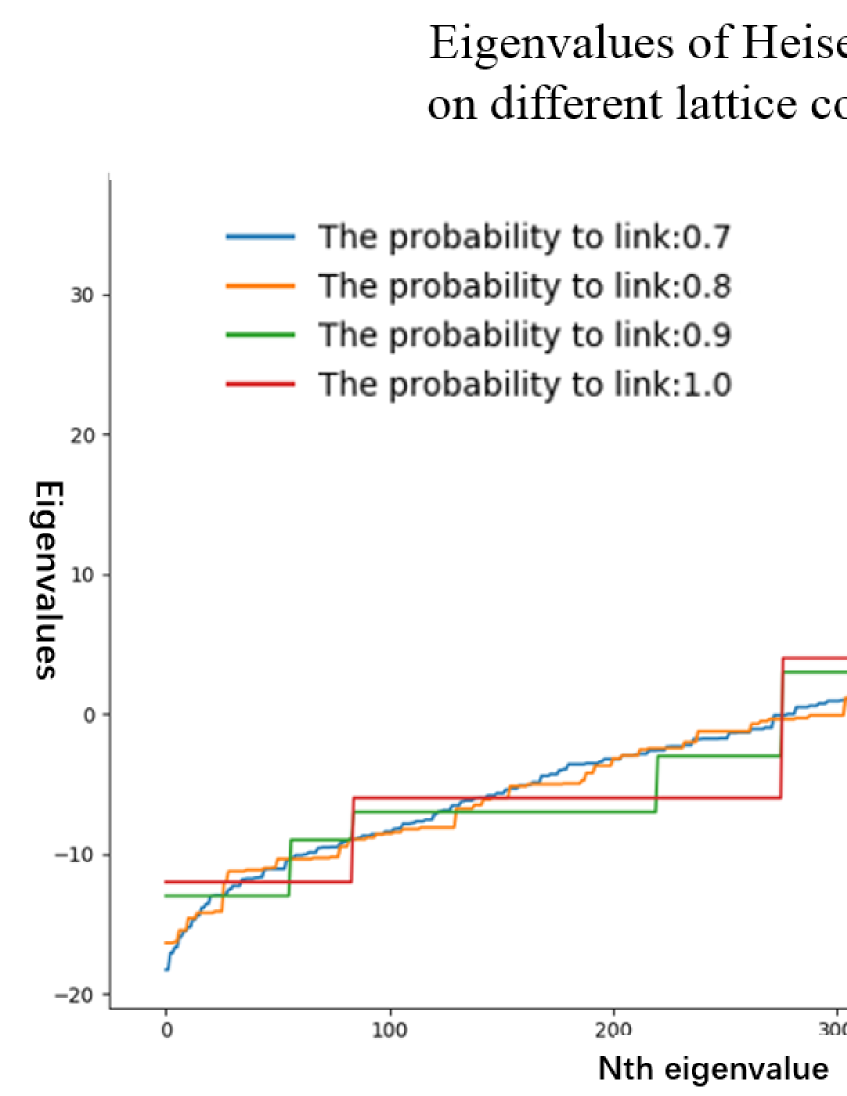
Figure 4: The eigenvalue of Heisenberg model consisting of $9$ particles on networks with random links. In a network, for any two particles, there is a probability to form a link between them.

Fig. (5) shows the number of distinct eigenvalues of Heisenberg models consisting of $N$ particles on networks with different number of links. It shows the tendency that degeneracy of eigenstates increases with the increase of the number of links when the number of links is relatively large.

To be notice that the number of distinct eigenvalues is not strictly monotonic decreasing as the number of links in the networks, see Fig. (5), because the number of links and how the links are formed decide the eigenvalues simultaneously. Here, we only consider the number of links in the networks.

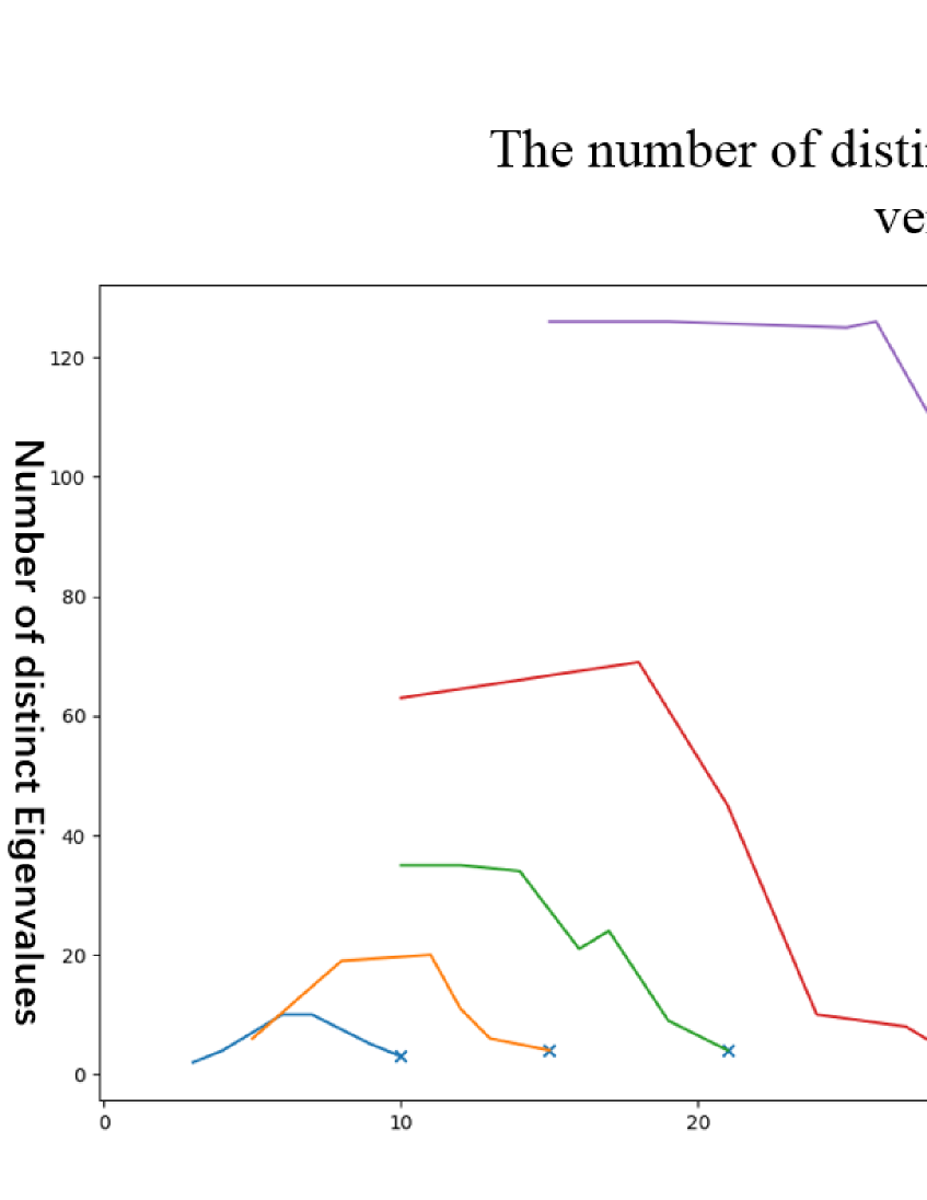
Figure 5: degeneracy of eigenstates of Heisenberg models consisting of different numbers of particles on lattice with different numbers of links. degeneracy here is revealed on the number of distinct eigenvalues.

The random walk. Here, we construct random walks on networks with different modes of links. For example, the matrix of a random walk on a one-dimensional lattice configuration consists of $5$ positions reads

$$\left(\begin{array}[c]{ccccc}0&\frac{1}{2}&0&0&\frac{1}{2}\\ \frac{1}{2}&0&\frac{1}{2}&0&0\\ 0&\frac{1}{2}&0&\frac{1}{2}&0\\ 0&0&\frac{1}{2}&0&\frac{1}{2}\\ \frac{1}{2}&0&0&\frac{1}{2}&0\end{array}\right),$$ (4.2)

where periodic boundary conditions are applied. On a one-dimensional lattice configuration, one can only go left or right with equal probability $1/2$. The random walk on a one-dimensional lattice configuration with a hole at position $1$ reads

$$\left(\begin{array}[c]{ccccc}0&0&0&0&0\\ 0&0&1&0&0\\ 0&\frac{1}{2}&0&\frac{1}{2}&0\\ 0&0&\frac{1}{2}&0&\frac{1}{2}\\ 0&0&0&1&0\end{array}\right),$$ (4.3)

where a hole means that any links to the hole is forbidden. Under such assumptions, one can not reach a hole. Thus, the probability to reach a hole is $0$. as shown in Table. (1) and Fig. (6), especially in three-dimension spaces, degeneracy of eigenstates increases with the number of links in the networks. The number of links is adjusted by changing the number of holes in the network.

Table 1: The number of distinct eigenvalues of random walks on different lattice configurations.

Shape	Position of holes	Number of links	Number of distinct eigenvalues
$1\times 25$	$-$	$25$	$13$
$1\times 25$	$4$	$23$	$25$
$1\times 25$	$2$ and $9$	$21$	$21$
$1\times 25$	$3$, $8$, and $13$	$19$	$17$
$5\times 5$	$-$	$50$	$6$
$5\times 5$	$(1,4)$	$46$	$17$
$5\times 5$	$(1,2)$ and $(2,4)$	$42$	$23$
$5\times 5$	$(1,3)$, $(2,3)$, and $(3,3)$	$40$	$21$
$3\times 3\times 3$	$-$	$81$	$4$
$3\times 3\times 3$	$(2,1,1)$	$75$	$8$
$3\times 3\times 3$	$(1,2,1)$ and $(3,3,1)$	$69$	$15$
$3\times 3\times 3$	$(2,2,1)$, $(3,3,1)$, $(3,3,2)$, and $(2,3,3)$	$59$	$16$

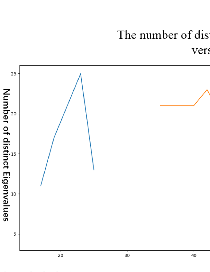
Figure 6: degeneracy of eigenstates of random walks on lattice configurations with different numbers of links. degeneracy here is revealed on the number of distinct eigenvalues.

4.2 The highest degeneracy of eigenstates of a lattice model

In Sec. 4.1, it shows that degeneracy of eigenvalues increases with the number of links in a network. That is, models on configurations with larger number of interacting particle-pairs have higher degeneracy of eigenstates. In this section, we propose the assumption that the lattice model with interactions between all particle-pairs, such as the generalized model proposed in Sec. 3.2, should have the highest degeneracy of eigenstates.

The highest degeneracy of eigenstates of the generalized Heisenberg model. For the generalized Heisenberg model consisting of $N$ particles with the dimension of single-particle-Hilbert space $m$, by using Eq. (3.21), the number of distinct eigenvalues is $P(N,m)$, where $P(N,m)$ is the restrict integer partition number [19] that is the number of ways to express $N$ as sum of other integers with the number of summands no larger than $m$. It is because one irreducible representation gives a distinct eigenvalue of Casimir operator and thus gives a distinct eigenvalue of the system. The irreducible representation is labeled by a set of number $\left(a\right)=\left(a_{1},a_{2},...,a_{m}\right)$ with $a_{1}\geqslant a_{2}\geqslant...\geqslant a_{m}\geqslant 0$ [17]. The summation of $\left(a\right)$ is $N$, thus, the number of $\left(a\right)$ equals the number of ways to represent $N$ in terms of other integers the number of summands smaller than $m$, that is $P(N,m)$. as shown in Fig. (7).

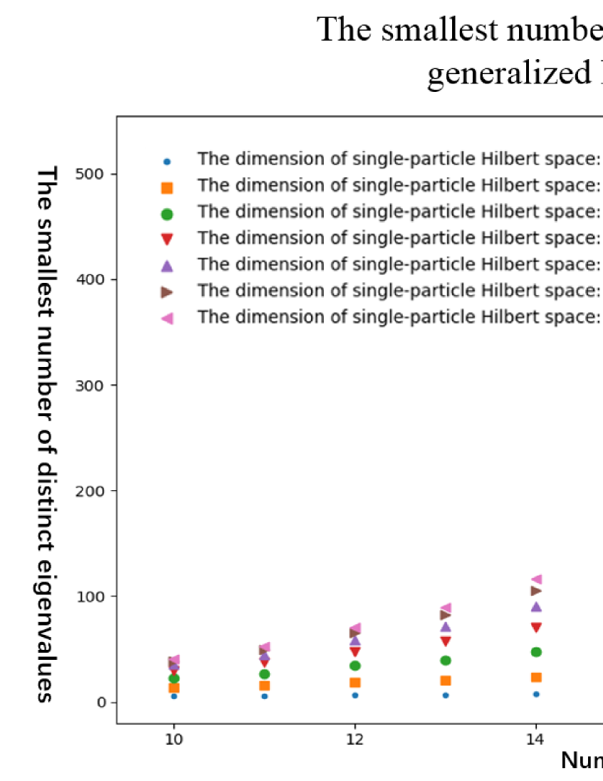
Figure 7: The smallest number of distinct eigenvalues of the generalized Heisenberg model.

For these cases, the average degeneracy of an energy level reads $m^{N}/P(N,m)$. For example, setting $m=3$ and $N=6$, the smallest number of distinct eigenvalues is $P(N,m)=7$, the average degeneracy is $104.14$. as shown in Table. (2), the average degeneracy of an energy level in creases fast with the number of particles or the dimension of single-particle Hilbert space.

Table 2: The average degeneracy of an energy level at the upper limit of energy level degeneracy.

The dimension of single-particle Hilbert space	Number of particles	The average degeneracy
$2$	$5$	$10.7$
$2$	$6$	$16.0$
$2$	$7$	$32.0$
$2$	$8$	$51.2$
$2$	$9$	$102.4$
$2$	$10$	$170.7$
$3$	$5$	$48.6$
$3$	$6$	$104.1$
$3$	$7$	$273.4$
$3$	$8$	$656.1$
$3$	$9$	$1640.3$
$3$	$10$	$4217.8$

5 Conclusions and discussions

The difficulty of solving the interacting quantum many-body system is due to the properties of the space configuration [20, 21, 22] and the interaction mode between inter-particles including the classical interaction and the quantum exchange interaction [23, 24, 25, 26]. Few models of quantum interacting many-body systems could be solved exactly in reality. Common practices are simplifying the models or using approximation methods instead of solving the system directly, we conclude that to investigate the system from the perspective of properties of the space and symmetries of the system is useful and effective.

In this paper, we consider models on lattice configurations with arbitrary numbers of interacting particle-pairs by converting the lattice configurations into networks with different modes of links. There are three main purposes of our work: (1) we introduce a group theory method to solve the Heisenberg model on lattice configurations with interactions between all particle-pairs by revealing the relation between the Casimir operator of the unitary group and the conjugacy-class operator of the permutation group. (2) We generalize the Heisenberg model by this proposed relation and thus give a series of exactly solvable models. (3) We show that degeneracy of the eigenvalue increases with the number of interacting particle-pairs. Thus, there is a highest degeneracy of eigenstates of a lattice model. The generalized Heisenberg model is a model on lattice configurations with interactions between all particle-pairs, and thus have the highest degeneracy of the eigenvalue among lattice models. The smallest number of distinct eigenvalues for the generalized Heisenberg model is a restrict integer partition function.

6 Acknowledgments

We are very indebted to Dr Yong Xie and Dr Guanwen Fang for their encouragements. This work is supported by the Fundamental Research Funds For the Central Universities No.2020JKF306.

References

- [1] R. J. Baxter, Exactly solved models in statistical mechanics. Elsevier, 2016.
- [2] L. Reichl, A Modern Course in Statistical Physics. Physics textbook. Wiley, 2009.
- [3] R. Pathria, Statistical Mechanics. Elsevier Science, 2011.
- [4] V. Galitski and I. B. Spielman, Spin–orbit coupling in quantum gases, Nature 494 (2013), no. 7435 49–54.
- [5] N. Goldman, G. Juzeliūnas, P. Öhberg, and I. B. Spielman, Light-induced gauge fields for ultracold atoms, Reports on Progress in Physics 77 (2014), no. 12 126401.
- [6] N. Crampé, E. Ragoucy, L. Alonzi, et al., Coordinate bethe ansatz for spin s xxx model, SIGMA. Symmetry, Integrability and Geometry: Methods and Applications 7 (2011) 006.
- [7] M. Arnesen, S. Bose, and V. Vedral, Natural thermal and magnetic entanglement in the 1d heisenberg model, Physical Review Letters 87 (2001), no. 1 017901.
- [8] A. W. Sandvik, Finite-size scaling of the ground-state parameters of the two-dimensional heisenberg model, Physical Review B 56 (1997), no. 18 11678.
- [9] A. Bougourzi, M. Couture, and M. Kacir, Exact two-spinon dynamical correlation function of the one-dimensional heisenberg model, Physical Review B 54 (1996), no. 18 R12669.
- [10] S. Belliard and N. Crampé, Heisenberg xxx model with general boundaries: eigenvectors from algebraic bethe ansatz, arXiv preprint arXiv:1309.6165 (2013).
- [11] A. Läuchli, F. Mila, and K. Penc, Quadrupolar phases of the s= 1 bilinear-biquadratic heisenberg model on the triangular lattice, Physical review letters 97 (2006), no. 8 087205.
- [12] P. Sindzingre, N. Shannon, and T. Momoi, Phase diagram of the spin-1/2 j1-j2-j3 heisenberg model on the square lattice, in Journal of Physics: Conference Series, vol. 200, p. 022058, IOP Publishing, 2010.
- [13] D. Braess, Finite elements: Theory, fast solvers, and applications in solid mechanics. Cambridge University Press, 2007.
- [14] O. C. Zienkiewicz, R. L. Taylor, R. L. Taylor, and R. L. Taylor, The finite element method: solid mechanics, vol. 2. Butterworth-heinemann, 2000.
- [15] R. Feynman, Statistical mechanics: a set of lectures (advanced book classics), .
- [16] L. Litinskii and B. Kryzhanovsky, Eigenvalues of ising connection matrix with long-range interaction, Physica A: Statistical Mechanics and its Applications 558 (2020) 124929.
- [17] F. Iachello, Lie algebras and applications, vol. 12. Springer, 2006.
- [18] J.-Q. Chen, J. Ping, and F. Wang, Group representation theory for physicists. World Scientific Publishing Company, 2002.
- [19] C.-C. Zhou and W.-S. Dai, A statistical mechanical approach to restricted integer partition functions, Journal of Statistical Mechanics: Theory and Experiment 2018 (2018), no. 5 053111.
- [20] X.-G. Wen, Quantum field theory of many-body systems: from the origin of sound to an origin of light and electrons. Oxford University Press on Demand, 2004.
- [21] N. Fläschner, D. Vogel, M. Tarnowski, B. Rem, D.-S. Lühmann, M. Heyl, J. Budich, L. Mathey, K. Sengstock, and C. Weitenberg, Observation of dynamical vortices after quenches in a system with topology, Nature Physics 14 (2018), no. 3 265–268.
- [22] L. Stenzel, A. L. Hayward, C. Hubig, U. Schollwöck, and F. Heidrich-Meisner, Quantum phases and topological properties of interacting fermions in one-dimensional superlattices, Physical Review A 99 (2019), no. 5 053614.
- [23] W.-S. Dai and M. Xie, Interacting quantum gases in confined space: Two-and three-dimensional equations of state, Journal of Mathematical Physics 48 (2007), no. 12 123302.
- [24] W. Dai and M. Xie, Hard-sphere gases as ideal gases with multi-core boundaries: An approach to two-and three-dimensional interacting gases, EPL (Europhysics Letters) 72 (2005), no. 6 887.
- [25] C.-C. Zhou and W.-S. Dai, Canonical partition functions: ideal quantum gases, interacting classical gases, and interacting quantum gases, Journal of Statistical Mechanics: Theory and Experiment 2018 (2018), no. 2 023105.
- [26] C.-C. Zhou and W.-S. Dai, Calculating eigenvalues of many-body systems from partition functions, Journal of Statistical Mechanics: Theory and Experiment 2018 (2018), no. 8 083103.