Dirac magnons pairing via pumping
Vladimir A. Zyuzin
Nordita, KTH Royal Institute of Technology and Stockholm University, Roslagstullsbacken 23, SE-106 91 Stockholm, Sweden
Abstract
We study pumping of magnons to the Dirac points of magnon’s Brillouin zone of a ferromagnet on a honeycomb lattice.
In particular, we consider second-order Suhl process, when due to interaction between magnons, a pair of magnons is created due to absorption of two electromagnetic wave quanta.
We introduce a bosonic analog of the Cooper ladder for the magnon pair, which is shown to enhance the pairing of magnons at the Dirac points.
As a result of pairing of the Dirac magnons, the system becomes unstable towards formation of a magnetic state with zero or reduced magnetization - the Dirac magnon paired state.
In this case the resonant frequency of the pump equals to that of energy of the Dirac points.
Our estimates suggest that the Dirac magnon paired state can be found in the CrBr3 3
Magnons are fluctuations about the spontaneous magnetic order.
Typically two types of magnons are distinguished based on the magnetic structure, ferromagnetic or antiferromagnetic. The two have different low-energy, low-momentum dispersion, regardless of the lattice structure of the magnetic structure. Ferromagnetic magnons are quadratic in momentum, while antiferromagnetic are linear (for example, see ABP1967 ; Auerbach ; Rezende Onose2010 ; ZhangPRB2013 ZhangPRB2013 ; Katsura2010 ; MookHenkMertig ; HirschbergerPRL2015 ; KovalevZyuzin MaksimovChernyshev ; Fransson ; Owerre2016a ; Owerre2016b ; Kim2016 ; KovalevZyuzinLi ; Pershoguba ; YelonSilberglitt ; HoneycombPRX2018 ; HoneycombPRX2020 Fransson Onose2010 ; Katsura2010 ; Owerre2016b KovalevZyuzin KovalevZyuzinLi
In this Letter we find another unique Dirac magnons property revealed under the second-order Suhl magnon pumping process Suhl1957 ; ZakharovLvovStarobinets ; Rezende ; ABP1967 1 2 1 Onose2010 HirschbergerPRL2015 YelonSilberglitt ; HoneycombPRX2018 ; HoneycombPRX2020 3 YelonSilberglitt
To demonstrate the effect, let us study a model of insulating ferromagnet in which spins of length S 𝑆 S 1 z 𝑧 z z − limit-from 𝑧 z- Ω Ω \Omega
H = − J ∑ ⟨ i j ⟩ 𝐒 i 𝐒 j + Γ ∑ i [ S i x cos ( Ω t ) + S i y sin ( Ω t ) ] , 𝐻 𝐽 subscript delimited-⟨⟩ 𝑖 𝑗 subscript 𝐒 𝑖 subscript 𝐒 𝑗 Γ subscript 𝑖 delimited-[] subscript superscript 𝑆 𝑥 𝑖 Ω 𝑡 subscript superscript 𝑆 𝑦 𝑖 Ω 𝑡 \displaystyle H=-J\sum_{\langle ij\rangle}{\bf S}_{i}{\bf S}_{j}+\Gamma\sum_{i}\left[S^{x}_{i}\cos(\Omega t)+S^{y}_{i}\sin(\Omega t)\right], (1)
where J > 0 𝐽 0 J>0 Γ Γ \Gamma S i ± = S i x ± i S i y superscript subscript 𝑆 𝑖 plus-or-minus plus-or-minus superscript subscript 𝑆 𝑖 𝑥 𝑖 superscript subscript 𝑆 𝑖 𝑦 S_{i}^{\pm}=S_{i}^{x}\pm iS_{i}^{y} S i z superscript subscript 𝑆 𝑖 𝑧 S_{i}^{z} S i + = 2 S − a i † a i a i superscript subscript 𝑆 𝑖 2 𝑆 superscript subscript 𝑎 𝑖 † subscript 𝑎 𝑖 subscript 𝑎 𝑖 S_{i}^{+}=\sqrt{2S-a_{i}^{{\dagger}}a_{i}}a_{i} S i − = a i † 2 S − a i † a i superscript subscript 𝑆 𝑖 superscript subscript 𝑎 𝑖 † 2 𝑆 superscript subscript 𝑎 𝑖 † subscript 𝑎 𝑖 S_{i}^{-}=a_{i}^{{\dagger}}\sqrt{2S-a_{i}^{{\dagger}}a_{i}} S i z = S − a i † a i superscript subscript 𝑆 𝑖 𝑧 𝑆 superscript subscript 𝑎 𝑖 † subscript 𝑎 𝑖 S_{i}^{z}=S-a_{i}^{{\dagger}}a_{i} [ a i , a j † ] = δ i , j subscript 𝑎 𝑖 superscript subscript 𝑎 𝑗 † subscript 𝛿 𝑖 𝑗
[a_{i},a_{j}^{{\dagger}}]=\delta_{i,j} b i subscript 𝑏 𝑖 b_{i} b i † superscript subscript 𝑏 𝑖 † b_{i}^{{\dagger}}
In the space of elements of the honeycomb’s unit cell, in which case the boson operators are defined by Ψ 𝐤 † = ( a 𝐤 † , b 𝐤 † ) superscript subscript Ψ 𝐤 † superscript subscript 𝑎 𝐤 † superscript subscript 𝑏 𝐤 † \Psi_{\bf k}^{\dagger}=(a_{\bf k}^{{\dagger}},~{}b_{\bf k}^{{\dagger}})
H 0 = S J ∫ 𝐤 Ψ 𝐤 † [ 3 − γ 𝐤 − γ 𝐤 ∗ 3 ] Ψ 𝐤 ≡ ∫ 𝐤 Ψ 𝐤 † [ H ^ 0 ] 𝐤 Ψ 𝐤 , subscript 𝐻 0 𝑆 𝐽 subscript 𝐤 superscript subscript Ψ 𝐤 † delimited-[] 3 subscript 𝛾 𝐤 superscript subscript 𝛾 𝐤 3 subscript Ψ 𝐤 subscript 𝐤 superscript subscript Ψ 𝐤 † subscript delimited-[] subscript ^ 𝐻 0 𝐤 subscript Ψ 𝐤 \displaystyle H_{0}=SJ\int_{\bf k}\Psi_{\bf k}^{\dagger}\left[\begin{array}[]{cc}3&-\gamma_{\bf k}\\
-\gamma_{\bf k}^{*}&3\end{array}\right]\Psi_{\bf k}\equiv\int_{\bf k}\Psi_{\bf k}^{\dagger}[\hat{H}_{0}]_{\bf k}\Psi_{\bf k}, (4)
where γ 𝐤 = ∑ i = 1 , 2 , 3 e i 𝐤 𝝉 i = 2 e i k x 2 3 cos ( k y 2 ) + e − i k x 3 subscript 𝛾 𝐤 subscript 𝑖 1 2 3
superscript 𝑒 𝑖 𝐤 subscript 𝝉 𝑖 2 superscript 𝑒 𝑖 subscript 𝑘 𝑥 2 3 subscript 𝑘 𝑦 2 superscript 𝑒 𝑖 subscript 𝑘 𝑥 3 \gamma_{\bf k}=\sum_{i=1,2,3}e^{i{\bf k}{\bm{\tau}}_{i}}=2e^{i\frac{k_{x}}{2\sqrt{3}}}\cos\left(\frac{k_{y}}{2}\right)+e^{-i\frac{k_{x}}{\sqrt{3}}} 1 ∫ 𝐤 ≡ ∫ d 𝐤 ( 2 π ) 2 subscript 𝐤 𝑑 𝐤 superscript 2 𝜋 2 \int_{\bf k}\equiv\int\frac{d{\bf k}}{(2\pi)^{2}} ε ± ; 𝐤 = S J ( 3 ± | γ 𝐤 | ) subscript 𝜀 plus-or-minus 𝐤
𝑆 𝐽 plus-or-minus 3 subscript 𝛾 𝐤 \varepsilon_{\pm;{\bf k}}=SJ\left(3\pm|\gamma_{\bf k}|\right) φ ± = 1 2 [ ∓ γ 𝐤 | γ 𝐤 | , 1 ] T subscript 𝜑 plus-or-minus 1 2 superscript minus-or-plus subscript 𝛾 𝐤 subscript 𝛾 𝐤 1 T \varphi_{\pm}=\frac{1}{\sqrt{2}}[\mp\frac{\gamma_{\bf k}}{|\gamma_{\bf k}|},~{}1]^{\mathrm{T}} 𝐊 = ( 0 , − 4 π 3 ) 𝐊 0 4 𝜋 3 {\bf K}=(0,-\frac{4\pi}{3}) 𝐊 ′ = ( 0 , 4 π 3 ) superscript 𝐊 ′ 0 4 𝜋 3 {\bf K}^{\prime}=(0,\frac{4\pi}{3}) ε ± ; 𝐤 = 3 S J subscript 𝜀 plus-or-minus 𝐤
3 𝑆 𝐽 \varepsilon_{\pm;{\bf k}}=3SJ
H int = − J ∫ { 𝐤 } δ { 𝐤 } γ 𝐤 4 − 𝐤 3 a 𝐤 1 † b 𝐤 3 † a 𝐤 2 b 𝐤 4 subscript 𝐻 int 𝐽 subscript 𝐤 subscript 𝛿 𝐤 subscript 𝛾 subscript 𝐤 4 subscript 𝐤 3 superscript subscript 𝑎 subscript 𝐤 1 † superscript subscript 𝑏 subscript 𝐤 3 † subscript 𝑎 subscript 𝐤 2 subscript 𝑏 subscript 𝐤 4 \displaystyle H_{\mathrm{int}}=-J\int_{\{{\bf k}\}}\delta_{\{{\bf k}\}}\gamma_{{\bf k}_{4}-{\bf k}_{3}}a_{{\bf k}_{1}}^{{\dagger}}b_{{\bf k}_{3}}^{{\dagger}}a_{{\bf k}_{2}}b_{{\bf k}_{4}} (5)
+ J 4 ∫ { 𝐤 } δ { 𝐤 } [ γ 𝐤 3 ∗ a 𝐤 1 † b 𝐤 3 † a 𝐤 2 a 𝐤 4 + γ 𝐤 3 a 𝐤 2 † a 𝐤 4 † a 𝐤 1 b 𝐤 3 ] 𝐽 4 subscript 𝐤 subscript 𝛿 𝐤 delimited-[] superscript subscript 𝛾 subscript 𝐤 3 superscript subscript 𝑎 subscript 𝐤 1 † superscript subscript 𝑏 subscript 𝐤 3 † subscript 𝑎 subscript 𝐤 2 subscript 𝑎 subscript 𝐤 4 subscript 𝛾 subscript 𝐤 3 superscript subscript 𝑎 subscript 𝐤 2 † superscript subscript 𝑎 subscript 𝐤 4 † subscript 𝑎 subscript 𝐤 1 subscript 𝑏 subscript 𝐤 3 \displaystyle+\frac{J}{4}\int_{\{{\bf k}\}}\delta_{\{{\bf k}\}}\left[\gamma_{{\bf k}_{3}}^{*}a_{{\bf k}_{1}}^{{\dagger}}b_{{\bf k}_{3}}^{{\dagger}}a_{{\bf k}_{2}}a_{{\bf k}_{4}}+\gamma_{{\bf k}_{3}}a_{{\bf k}_{2}}^{{\dagger}}a_{{\bf k}_{4}}^{{\dagger}}a_{{\bf k}_{1}}b_{{\bf k}_{3}}\right]
+ J 4 ∫ { 𝐤 } δ { 𝐤 } [ γ 𝐤 1 a 𝐤 1 † b 𝐤 3 † b 𝐤 2 b 𝐤 4 + γ 𝐤 1 ∗ b 𝐤 2 † b 𝐤 4 † a 𝐤 1 b 𝐤 3 ] , 𝐽 4 subscript 𝐤 subscript 𝛿 𝐤 delimited-[] subscript 𝛾 subscript 𝐤 1 superscript subscript 𝑎 subscript 𝐤 1 † superscript subscript 𝑏 subscript 𝐤 3 † subscript 𝑏 subscript 𝐤 2 subscript 𝑏 subscript 𝐤 4 superscript subscript 𝛾 subscript 𝐤 1 superscript subscript 𝑏 subscript 𝐤 2 † superscript subscript 𝑏 subscript 𝐤 4 † subscript 𝑎 subscript 𝐤 1 subscript 𝑏 subscript 𝐤 3 \displaystyle+\frac{J}{4}\int_{\{{\bf k}\}}\delta_{\{{\bf k}\}}\left[\gamma_{{\bf k}_{1}}a_{{\bf k}_{1}}^{{\dagger}}b_{{\bf k}_{3}}^{{\dagger}}b_{{\bf k}_{2}}b_{{\bf k}_{4}}+\gamma_{{\bf k}_{1}}^{*}b_{{\bf k}_{2}}^{{\dagger}}b_{{\bf k}_{4}}^{{\dagger}}a_{{\bf k}_{1}}b_{{\bf k}_{3}}\right],
where δ { 𝐤 } ≡ δ 𝐤 1 − 𝐤 2 , 𝐤 4 − 𝐤 3 subscript 𝛿 𝐤 subscript 𝛿 subscript 𝐤 1 subscript 𝐤 2 subscript 𝐤 4 subscript 𝐤 3
\delta_{\{{\bf k}\}}\equiv\delta_{{\bf k}_{1}-{\bf k}_{2},{\bf k}_{4}-{\bf k}_{3}} ∫ { 𝐤 } subscript 𝐤 \int_{\{{\bf k}\}} Ω Ω \Omega
H pump = Γ S 2 [ ( a 0 + b 0 ) e − i Ω t + ( a 0 † + b 0 † ) e i Ω t ] , subscript 𝐻 pump Γ 𝑆 2 delimited-[] subscript 𝑎 0 subscript 𝑏 0 superscript 𝑒 𝑖 Ω 𝑡 subscript superscript 𝑎 † 0 subscript superscript 𝑏 † 0 superscript 𝑒 𝑖 Ω 𝑡 \displaystyle H_{\mathrm{pump}}=\frac{\Gamma\sqrt{S}}{\sqrt{2}}\left[(a_{0}+b_{0})e^{-i\Omega t}+(a^{{\dagger}}_{0}+b^{{\dagger}}_{0})e^{i\Omega t}\right], (6)
where a 0 ≡ a 𝐤 = 0 subscript 𝑎 0 subscript 𝑎 𝐤 0 a_{0}\equiv a_{{\bf k}=0} b 0 subscript 𝑏 0 b_{0} 6 4 5 a 𝐤 , b 𝐤 subscript 𝑎 𝐤 subscript 𝑏 𝐤
a_{\bf k},b_{\bf k} Ψ α ; 𝐤 ; ϵ , Ψ β ; 𝐤 ; ϵ subscript Ψ 𝛼 𝐤 italic-ϵ
subscript Ψ 𝛽 𝐤 italic-ϵ
\Psi_{\alpha;{\bf k};\epsilon},\Psi_{\beta;{\bf k};\epsilon} ϵ italic-ϵ \epsilon a 𝐤 † , b 𝐤 † subscript superscript 𝑎 † 𝐤 subscript superscript 𝑏 † 𝐤
a^{{\dagger}}_{\bf k},b^{{\dagger}}_{\bf k} Ψ ¯ α ; 𝐤 ; ϵ , Ψ ¯ β ; 𝐤 ; ϵ subscript ¯ Ψ 𝛼 𝐤 italic-ϵ
subscript ¯ Ψ 𝛽 𝐤 italic-ϵ
\bar{\Psi}_{\alpha;{\bf k};\epsilon},\bar{\Psi}_{\beta;{\bf k};\epsilon} cl cl \mathrm{cl} q q \mathrm{q} SM Kamenev 6
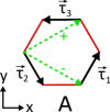
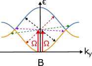
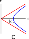
Figure 1: A. Schematics of the honeycomb lattice. Vectors connecting the nearest neighbor cites are 𝝉 1 = 1 2 ( 1 3 , 1 ) subscript 𝝉 1 1 2 1 3 1 {\bm{\tau}}_{1}=\frac{1}{2}\left(\frac{1}{\sqrt{3}},1\right) 𝝉 2 = 1 2 ( 1 3 , − 1 ) subscript 𝝉 2 1 2 1 3 1 {\bm{\tau}}_{2}=\frac{1}{2}\left(\frac{1}{\sqrt{3}},-1\right) 𝝉 3 = 1 3 ( − 1 , 0 ) subscript 𝝉 3 1 3 1 0 {\bm{\tau}}_{3}=\frac{1}{\sqrt{3}}(-1,0) k x = 0 subscript 𝑘 𝑥 0 k_{x}=0 𝐤 𝐤 {\bf k} Ω + ϵ Ω italic-ϵ \Omega+\epsilon − 𝐤 𝐤 -{\bf k} Ω − ϵ Ω italic-ϵ \Omega-\epsilon Ω = 3 S J Ω 3 𝑆 𝐽 \Omega=3SJ k th subscript 𝑘 th k_{\mathrm{th}} 16
We write the advanced part of the Lagrangian describing non-interacting magnons defined by Eq. (4 ϵ = Ω italic-ϵ Ω \epsilon=\Omega 𝐤 = 0 𝐤 0 {\bf k}=0
ℒ 0 , Ω A = ∑ m , n Ψ ¯ m , 0 , Ω cl ℒ ^ m n , 0 , Ω A Ψ n , 0 , Ω q − Γ S ∑ n Ψ n , 0 , Ω q , subscript superscript ℒ A 0 Ω
subscript 𝑚 𝑛
subscript superscript ¯ Ψ cl 𝑚 0 Ω
subscript superscript ^ ℒ A 𝑚 𝑛 0 Ω
subscript superscript Ψ q 𝑛 0 Ω
Γ 𝑆 subscript 𝑛 subscript superscript Ψ q 𝑛 0 Ω
\displaystyle{\cal L}^{\mathrm{A}}_{0,\Omega}=\sum_{m,n}\bar{\Psi}^{\mathrm{cl}}_{m,0,\Omega}\hat{{\cal L}}^{\mathrm{A}}_{mn,0,\Omega}\Psi^{\mathrm{q}}_{n,0,\Omega}-\Gamma\sqrt{S}\sum_{n}\Psi^{\mathrm{q}}_{n,0,\Omega}, (7)
where ℒ ^ m n , 𝐤 , Ω A = ( Ω − i 0 ) δ m n − [ H ^ 0 ] m n , 𝐤 subscript superscript ^ ℒ A 𝑚 𝑛 𝐤 Ω
Ω 𝑖 0 subscript 𝛿 𝑚 𝑛 subscript delimited-[] subscript ^ 𝐻 0 𝑚 𝑛 𝐤
\hat{{\cal L}}^{\mathrm{A}}_{mn,{\bf k},\Omega}=(\Omega-i0)\delta_{mn}-[\hat{H}_{0}]_{mn,{\bf k}} m , n = { α , β } 𝑚 𝑛
𝛼 𝛽 m,n=\{\alpha,\beta\} Ψ n , 0 , Ω q subscript superscript Ψ q 𝑛 0 Ω
\Psi^{\mathrm{q}}_{n,0,\Omega}
Ψ ¯ α , 0 , Ω cl → Ψ ¯ α , 0 , Ω cl + x A , Ψ ¯ β , 0 , Ω cl → Ψ ¯ β , 0 , Ω cl + y A , formulae-sequence → subscript superscript ¯ Ψ cl 𝛼 0 Ω
subscript superscript ¯ Ψ cl 𝛼 0 Ω
subscript 𝑥 A → subscript superscript ¯ Ψ cl 𝛽 0 Ω
subscript superscript ¯ Ψ cl 𝛽 0 Ω
subscript 𝑦 A \displaystyle\bar{\Psi}^{\mathrm{cl}}_{\alpha,0,\Omega}\rightarrow\bar{\Psi}^{\mathrm{cl}}_{\alpha,0,\Omega}+x_{\mathrm{A}},~{}~{}~{}~{}\bar{\Psi}^{\mathrm{cl}}_{\beta,0,\Omega}\rightarrow\bar{\Psi}^{\mathrm{cl}}_{\beta,0,\Omega}+y_{\mathrm{A}}, (8)
where x A subscript 𝑥 A x_{\mathrm{A}} y A subscript 𝑦 A y_{\mathrm{A}}
x A = ℒ β α , 0 , Ω A − ℒ β β , 0 , Ω A ℒ α β , 0 , Ω A ℒ β α , 0 , Ω A − ℒ β β , 0 , Ω A ℒ α α , 0 , Ω A Γ S , subscript 𝑥 A subscript superscript ℒ A 𝛽 𝛼 0 Ω
subscript superscript ℒ A 𝛽 𝛽 0 Ω
subscript superscript ℒ A 𝛼 𝛽 0 Ω
subscript superscript ℒ A 𝛽 𝛼 0 Ω
subscript superscript ℒ A 𝛽 𝛽 0 Ω
subscript superscript ℒ A 𝛼 𝛼 0 Ω
Γ 𝑆 \displaystyle x_{\mathrm{A}}=\frac{{\cal L}^{\mathrm{A}}_{\beta\alpha,0,\Omega}-{\cal L}^{\mathrm{A}}_{\beta\beta,0,\Omega}}{{\cal L}^{\mathrm{A}}_{\alpha\beta,0,\Omega}{\cal L}^{\mathrm{A}}_{\beta\alpha,0,\Omega}-{\cal L}^{\mathrm{A}}_{\beta\beta,0,\Omega}{\cal L}^{\mathrm{A}}_{\alpha\alpha,0,\Omega}}\Gamma\sqrt{S}, (9)
y A = ℒ α β , 0 , Ω A − ℒ α α , 0 , Ω A ℒ α β , 0 , Ω A ℒ β α , 0 , Ω A − ℒ β β , 0 , Ω A ℒ α α , 0 , Ω A Γ S . subscript 𝑦 A subscript superscript ℒ A 𝛼 𝛽 0 Ω
subscript superscript ℒ A 𝛼 𝛼 0 Ω
subscript superscript ℒ A 𝛼 𝛽 0 Ω
subscript superscript ℒ A 𝛽 𝛼 0 Ω
subscript superscript ℒ A 𝛽 𝛽 0 Ω
subscript superscript ℒ A 𝛼 𝛼 0 Ω
Γ 𝑆 \displaystyle y_{\mathrm{A}}=\frac{{\cal L}^{\mathrm{A}}_{\alpha\beta,0,\Omega}-{\cal L}^{\mathrm{A}}_{\alpha\alpha,0,\Omega}}{{\cal L}^{\mathrm{A}}_{\alpha\beta,0,\Omega}{\cal L}^{\mathrm{A}}_{\beta\alpha,0,\Omega}-{\cal L}^{\mathrm{A}}_{\beta\beta,0,\Omega}{\cal L}^{\mathrm{A}}_{\alpha\alpha,0,\Omega}}\Gamma\sqrt{S}. (10)
The same procedure is performed for the retarded part of the action to take care of the − Γ S ∑ n Ψ ¯ n , 0 , Ω q Γ 𝑆 subscript 𝑛 subscript superscript ¯ Ψ q 𝑛 0 Ω
-\Gamma\sqrt{S}\sum_{n}\bar{\Psi}^{\mathrm{q}}_{n,0,\Omega} SM 5 Ω Ω \Omega 𝐤 = 0 𝐤 0 {\bf k}=0 SM ∝ Ψ ¯ n , 𝐤 , ϵ cl / q Ψ m , 𝐤 , ϵ q / cl proportional-to absent subscript superscript ¯ Ψ cl q 𝑛 𝐤 italic-ϵ
subscript superscript Ψ q cl 𝑚 𝐤 italic-ϵ
\propto\bar{\Psi}^{\mathrm{cl}/\mathrm{q}}_{n,{\bf k},\epsilon}\Psi^{\mathrm{q}/\mathrm{cl}}_{m,{\bf k},\epsilon} Suhl1957 ∝ Ψ ¯ n , 𝐤 , Ω + ϵ cl / q Ψ ¯ m , − 𝐤 , Ω − ϵ q / cl proportional-to absent subscript superscript ¯ Ψ cl q 𝑛 𝐤 Ω italic-ϵ
subscript superscript ¯ Ψ q cl 𝑚 𝐤 Ω italic-ϵ
\propto\bar{\Psi}^{\mathrm{cl}/\mathrm{q}}_{n,{\bf k},\Omega+\epsilon}\bar{\Psi}^{\mathrm{q}/\mathrm{cl}}_{m,-{\bf k},\Omega-\epsilon} 𝐤 , Ω + ϵ 𝐤 Ω italic-ϵ
{\bf k},\Omega+\epsilon − 𝐤 , Ω − ϵ 𝐤 Ω italic-ϵ
-{\bf k},\Omega-\epsilon 1
Let us now understand what will the creation of a magnon pair do to the system. Our calculations show that in the extended space of magnons, Φ ¯ 𝐤 , ϵ cl / q = 1 2 ( Ψ ¯ α , 𝐤 , Ω + ϵ cl / q , Ψ ¯ β , 𝐤 , Ω + ϵ cl / q , Ψ α , − 𝐤 , Ω − ϵ cl / q , Ψ β , − 𝐤 , Ω − ϵ cl / q ) subscript superscript ¯ Φ cl q 𝐤 italic-ϵ
1 2 subscript superscript ¯ Ψ cl q 𝛼 𝐤 Ω italic-ϵ
subscript superscript ¯ Ψ cl q 𝛽 𝐤 Ω italic-ϵ
subscript superscript Ψ cl q 𝛼 𝐤 Ω italic-ϵ
subscript superscript Ψ cl q 𝛽 𝐤 Ω italic-ϵ
\bar{\Phi}^{\mathrm{cl}/\mathrm{q}}_{{\bf k},\epsilon}=\frac{1}{\sqrt{2}}(\bar{\Psi}^{\mathrm{cl}/\mathrm{q}}_{\alpha,{\bf k},\Omega+\epsilon},\bar{\Psi}^{\mathrm{cl}/\mathrm{q}}_{\beta,{\bf k},\Omega+\epsilon},\Psi^{\mathrm{cl}/\mathrm{q}}_{\alpha,-{\bf k},\Omega-\epsilon},\Psi^{\mathrm{cl}/\mathrm{q}}_{\beta,-{\bf k},\Omega-\epsilon})
det det \displaystyle\mathrm{det} [ ζ + ϵ S J γ 𝐤 − Δ 2 γ 0 Δ 2 γ 𝐤 S J γ 𝐤 ∗ ζ + ϵ Δ 2 γ 𝐤 ∗ − Δ 2 γ 0 − Δ 2 γ 0 Δ 2 γ 𝐤 ζ − ϵ S J γ 𝐤 Δ 2 γ 𝐤 ∗ − Δ 2 γ 0 S J γ 𝐤 ∗ ζ − ϵ ] = 0 , delimited-[] 𝜁 italic-ϵ 𝑆 𝐽 subscript 𝛾 𝐤 superscript Δ 2 subscript 𝛾 0 superscript Δ 2 subscript 𝛾 𝐤 𝑆 𝐽 superscript subscript 𝛾 𝐤 𝜁 italic-ϵ superscript Δ 2 subscript superscript 𝛾 𝐤 superscript Δ 2 subscript 𝛾 0 superscript Δ 2 subscript 𝛾 0 superscript Δ 2 subscript 𝛾 𝐤 𝜁 italic-ϵ 𝑆 𝐽 subscript 𝛾 𝐤 superscript Δ 2 superscript subscript 𝛾 𝐤 superscript Δ 2 subscript 𝛾 0 𝑆 𝐽 superscript subscript 𝛾 𝐤 𝜁 italic-ϵ 0 \displaystyle\left[\begin{array}[]{cccc}\zeta+\epsilon&SJ\gamma_{\bf k}&-\Delta^{2}\gamma_{0}&\Delta^{2}\gamma_{{\bf k}}\\
SJ\gamma_{\bf k}^{*}&\zeta+\epsilon&\Delta^{2}\gamma^{*}_{{\bf k}}&-\Delta^{2}\gamma_{0}\\
-\Delta^{2}\gamma_{0}&\Delta^{2}\gamma_{{\bf k}}&\zeta-\epsilon&SJ\gamma_{\bf k}\\
\Delta^{2}\gamma_{{\bf k}}^{*}&-\Delta^{2}\gamma_{0}&SJ\gamma_{\bf k}^{*}&\zeta-\epsilon\end{array}\right]=0, (15)
where ζ = Ω − 3 S J 𝜁 Ω 3 𝑆 𝐽 \zeta=\Omega-3SJ γ 0 = 3 subscript 𝛾 0 3 \gamma_{0}=3 Δ 2 = J 4 ( Γ S 3 S J ) 2 superscript Δ 2 𝐽 4 superscript Γ 𝑆 3 𝑆 𝐽 2 \Delta^{2}=\frac{J}{4}\left(\frac{\Gamma\sqrt{S}}{3SJ}\right)^{2} ζ = 0 𝜁 0 \zeta=0 Δ 2 = J 4 ( Γ S 6 S J ) 2 superscript Δ 2 𝐽 4 superscript Γ 𝑆 6 𝑆 𝐽 2 \Delta^{2}=\frac{J}{4}\left(\frac{\Gamma\sqrt{S}}{6SJ}\right)^{2} ζ = ± 3 S J 𝜁 plus-or-minus 3 𝑆 𝐽 \zeta=\pm 3SJ 8 ϵ italic-ϵ \epsilon 15
ϵ ± ; 𝐤 2 = ( ζ ± S J | γ 𝐤 | ) 2 − Δ 4 ( γ 0 ∓ | γ 𝐤 | ) 2 . superscript subscript italic-ϵ plus-or-minus 𝐤
2 superscript plus-or-minus 𝜁 𝑆 𝐽 subscript 𝛾 𝐤 2 superscript Δ 4 superscript minus-or-plus subscript 𝛾 0 subscript 𝛾 𝐤 2 \displaystyle\epsilon_{\pm;{\bf k}}^{2}=(\zeta\pm SJ|\gamma_{\bf k}|)^{2}-\Delta^{4}(\gamma_{0}\mp|\gamma_{\bf k}|)^{2}. (16)
Therefore, the system of pumped interacting magnons will become unstable when ϵ ± ; 𝐤 2 < 0 superscript subscript italic-ϵ plus-or-minus 𝐤
2 0 \epsilon_{\pm;{\bf k}}^{2}<0
Let us first study a special case when pump’s frequency is Ω = 3 S J Ω 3 𝑆 𝐽 \Omega=3SJ ζ = 0 𝜁 0 \zeta=0 𝚪 = ( 0 , 0 ) 𝚪 0 0 {\bm{\Gamma}}=(0,0) | γ 𝐤 | ≈ 3 − k 2 4 subscript 𝛾 𝐤 3 superscript 𝑘 2 4 |\gamma_{\bf k}|\approx 3-\frac{k^{2}}{4} ϵ + ; 𝐤 2 = ( S J ) 2 ( 3 − k 2 4 ) 2 − 36 Δ 4 superscript subscript italic-ϵ 𝐤
2 superscript 𝑆 𝐽 2 superscript 3 superscript 𝑘 2 4 2 36 superscript Δ 4 \epsilon_{+;{\bf k}}^{2}=(SJ)^{2}\left(3-\frac{k^{2}}{4}\right)^{2}-36\Delta^{4} 𝚪 𝚪 {\bm{\Gamma}} S J > Δ 2 𝑆 𝐽 superscript Δ 2 SJ>\Delta^{2} 𝚪 𝚪 {\bm{\Gamma}} 𝐊 𝐊 {\bf K} 𝐊 ′ superscript 𝐊 ′ {\bf K}^{\prime} | γ 𝐤 | ≈ 3 2 k subscript 𝛾 𝐤 3 2 𝑘 |\gamma_{\bf k}|\approx\frac{\sqrt{3}}{2}k ϵ ± ; 𝐤 2 ≈ ( S J ) 2 3 4 k 2 − 9 Δ 4 superscript subscript italic-ϵ plus-or-minus 𝐤
2 superscript 𝑆 𝐽 2 3 4 superscript 𝑘 2 9 superscript Δ 4 \epsilon_{\pm;{\bf k}}^{2}\approx(SJ)^{2}\frac{3}{4}k^{2}-9\Delta^{4} k th = 2 3 Δ 2 S J subscript 𝑘 th 2 3 superscript Δ 2 𝑆 𝐽 k_{\mathrm{th}}=\frac{2\sqrt{3}\Delta^{2}}{SJ} k < k th 𝑘 subscript 𝑘 th k<k_{\mathrm{th}} 1
Having pumped the magnons to the Dirac points, let us now study their rescattering processes.
In the first order in interaction Eq. (5 2 BlochPRL1962 5 Pershoguba Δ 2 superscript Δ 2 \Delta^{2} 2 SM Δ 2 superscript Δ 2 \Delta^{2} 15 Δ 2 superscript Δ 2 \Delta^{2} ζ = 0 𝜁 0 \zeta=0
Δ 2 → Δ 2 1 − J J ~ [ 1 4 S + π 8 S ( T 3 S J ~ ) 2 ] , → superscript Δ 2 superscript Δ 2 1 𝐽 ~ 𝐽 delimited-[] 1 4 𝑆 𝜋 8 𝑆 superscript 𝑇 3 𝑆 ~ 𝐽 2 \displaystyle\Delta^{2}\rightarrow\frac{\Delta^{2}}{1-\frac{J}{\tilde{J}}\left[\frac{1}{4S}+\frac{\pi}{8S}\left(\frac{T}{3S\tilde{J}}\right)^{2}\right]}, (17)
where J ~ = J [ 1 − π 4 S ( T 3 S J ) 2 ] ~ 𝐽 𝐽 delimited-[] 1 𝜋 4 𝑆 superscript 𝑇 3 𝑆 𝐽 2 \tilde{J}=J\left[1-\frac{\pi}{4S}\left(\frac{T}{3SJ}\right)^{2}\right] 17 5 3 3 S = 3 2 𝑆 3 2 S=\frac{3}{2} YelonSilberglitt T ≃ T c ∼ 3 S J similar-to-or-equals 𝑇 subscript 𝑇 𝑐 similar-to 3 𝑆 𝐽 T\simeq T_{c}\sim 3SJ 17 Pershoguba ; BlochPRL1962 ; YelonSilberglitt S 𝑆 S 17
Figure 2: A. Hartree-Fock corrections to the dispersion of magnons. Wavy lines stand for the interaction defined in Eq. (5 Δ i j 2 subscript superscript Δ 2 𝑖 𝑗 \Delta^{2}_{ij} 15 Δ aa 2 = Δ bb 2 = − Δ 2 γ 0 subscript superscript Δ 2 aa subscript superscript Δ 2 bb superscript Δ 2 subscript 𝛾 0 \Delta^{2}_{\mathrm{aa}}=\Delta^{2}_{\mathrm{bb}}=-\Delta^{2}\gamma_{0} Δ ab 2 = ( Δ ba 2 ) ∗ = Δ 2 γ 𝐤 subscript superscript Δ 2 ab superscript subscript superscript Δ 2 ba superscript Δ 2 subscript 𝛾 𝐤 \Delta^{2}_{\mathrm{ab}}=(\Delta^{2}_{\mathrm{ba}})^{*}=\Delta^{2}\gamma_{\bf k}
Let us study the effect of Dzyaloshinskii-Moriya interaction of the H DMI = D ∑ ⟨ ⟨ i j ⟩ ⟩ ν i j [ 𝐒 i × 𝐒 j ] z subscript 𝐻 DMI 𝐷 subscript delimited-⟨⟩ delimited-⟨⟩ 𝑖 𝑗 subscript 𝜈 𝑖 𝑗 subscript delimited-[] subscript 𝐒 𝑖 subscript 𝐒 𝑗 𝑧 H_{\mathrm{DMI}}=D\sum_{\langle\langle ij\rangle\rangle}\nu_{ij}[{\bf S}_{i}\times{\bf S}_{j}]_{z} D 𝐷 D ⟨ ⟨ i j ⟩ ⟩ delimited-⟨⟩ delimited-⟨⟩ 𝑖 𝑗 \langle\langle ij\rangle\rangle ν i j = ± 1 subscript 𝜈 𝑖 𝑗 plus-or-minus 1 \nu_{ij}=\pm 1 1 ζ = 0 𝜁 0 \zeta=0
ϵ ± 2 = ( S J ) 2 3 4 k 2 + χ 2 − 9 Δ 4 , subscript superscript italic-ϵ 2 plus-or-minus superscript 𝑆 𝐽 2 3 4 superscript 𝑘 2 superscript 𝜒 2 9 superscript Δ 4 \displaystyle\epsilon^{2}_{\pm}=(SJ)^{2}\frac{3}{4}k^{2}+\chi^{2}-9\Delta^{4}, (18)
where χ = 3 3 S D 𝜒 3 3 𝑆 𝐷 \chi=3\sqrt{3}SD | χ | ≥ 3 Δ 2 𝜒 3 superscript Δ 2 |\chi|\geq 3\Delta^{2}
When ζ < 0 𝜁 0 \zeta<0 ϵ + ; 𝐤 2 superscript subscript italic-ϵ 𝐤
2 \epsilon_{+;{\bf k}}^{2} 𝚪 𝚪 {\bm{\Gamma}} | γ 𝐤 | ≈ 3 − k 2 4 subscript 𝛾 𝐤 3 superscript 𝑘 2 4 |\gamma_{\bf k}|\approx 3-\frac{k^{2}}{4} k th = Ω S J Δ 2 S J subscript 𝑘 th Ω 𝑆 𝐽 superscript Δ 2 𝑆 𝐽 k_{\mathrm{th}}=\sqrt{\frac{\Omega}{SJ}}\frac{\Delta^{2}}{SJ} 3 S J > ζ > 0 3 𝑆 𝐽 𝜁 0 3SJ>\zeta>0 ϵ − ; 𝐤 2 superscript subscript italic-ϵ 𝐤
2 \epsilon_{-;{\bf k}}^{2} ζ < 0 𝜁 0 \zeta<0 k th = 6 Δ 2 S J ( 3 S J − ζ ) subscript 𝑘 th 6 superscript Δ 2 𝑆 𝐽 3 𝑆 𝐽 𝜁 k_{\mathrm{th}}=\frac{6\Delta^{2}}{\sqrt{SJ(3SJ-\zeta)}} 3 S J − ζ > 3 2 Δ 2 3 𝑆 𝐽 𝜁 3 2 superscript Δ 2 3SJ-\zeta>\frac{3}{2}\Delta^{2} 𝚪 𝚪 {\bm{\Gamma}} k th = 2 6 Δ S J subscript 𝑘 th 2 6 Δ 𝑆 𝐽 k_{\mathrm{th}}=\frac{2\sqrt{6}\Delta}{\sqrt{SJ}} 3 S J − ζ < 3 2 Δ 2 3 𝑆 𝐽 𝜁 3 2 superscript Δ 2 3SJ-\zeta<\frac{3}{2}\Delta^{2} 𝚪 𝚪 {\bf\Gamma} 2 3 S J > ζ > 0 3 𝑆 𝐽 𝜁 0 3SJ>\zeta>0
Δ 2 → Δ 2 1 + 3 16 π S ln ( S J Λ 2 4 ( 3 S J − ζ ) ) + i 3 16 S , → superscript Δ 2 superscript Δ 2 1 3 16 𝜋 𝑆 𝑆 𝐽 superscript Λ 2 4 3 𝑆 𝐽 𝜁 𝑖 3 16 𝑆 \displaystyle\Delta^{2}\rightarrow\frac{\Delta^{2}}{1+\frac{3}{16\pi S}\ln\left(\frac{SJ\Lambda^{2}}{4(3SJ-\zeta)}\right)+i\frac{3}{16S}}, (19)
where Λ Λ \Lambda Ω → 6 S J → Ω 6 𝑆 𝐽 \Omega\rightarrow 6SJ Ω = 6 S J Ω 6 𝑆 𝐽 \Omega=6SJ
In addition to studied rescattering processes, one needs to include magnon decay rate, which originates due to interactions in second-order perturbation theory, to the main diagonal in the secular equation Eq. (15 Pershoguba 1 τ ∝ T 2 proportional-to 1 𝜏 superscript 𝑇 2 \frac{1}{\tau}\propto T^{2} ε + ; 𝐤 subscript 𝜀 𝐤
\varepsilon_{+;{\bf k}} 𝚪 𝚪 {\bm{\Gamma}} 17
There are two corollaries which can be made on the nature of the Dirac magnon paired state.
First of all, when the conditions for the instability are met (divergence of Eq. (17 Ω = 3 S J Ω 3 𝑆 𝐽 \Omega=3SJ 6 S 2 J 6 superscript 𝑆 2 𝐽 6S^{2}J 6 S J 6 𝑆 𝐽 6SJ S = 1 𝑆 1 S=1 S = 2 𝑆 2 S=2 Demokritov
In passing, let us discuss another possiblity of pumping the magnons. First note that in the honeycomb lattice there are two energy branches at the 𝚪 𝚪 {\bm{\Gamma}} ϵ + ; 0 = 6 S J subscript italic-ϵ 0
6 𝑆 𝐽 \epsilon_{+;0}=6SJ ϵ − ; 0 = 0 subscript italic-ϵ 0
0 \epsilon_{-;0}=0 Ω = 6 S J Ω 6 𝑆 𝐽 \Omega=6SJ 6 ϵ − ; 0 + Ω → ϵ + ; 0 → subscript italic-ϵ 0
Ω subscript italic-ϵ 0
\epsilon_{-;0}+\Omega\rightarrow\epsilon_{+;0} 15 16 ϵ + ; 0 subscript italic-ϵ 0
\epsilon_{+;0} ϵ + ; 0 + ϵ − ; 0 → ϵ + ; 𝐊 + ϵ − ; 𝐊 ′ → subscript italic-ϵ 0
subscript italic-ϵ 0
subscript italic-ϵ 𝐊
subscript italic-ϵ superscript 𝐊 ′
\epsilon_{+;0}+\epsilon_{-;0}\rightarrow\epsilon_{+;{\bf K}}+\epsilon_{-;{\bf K}^{\prime}} Demokritov ε + ; 𝐤 = 6 S J subscript 𝜀 𝐤
6 𝑆 𝐽 \varepsilon_{+;{\bf k}}=6SJ ε − ; 𝐤 = 0 subscript 𝜀 𝐤
0 \varepsilon_{-;{\bf k}}=0
To conclude, we studied second-order Suhl processes in a honeycomb ferromagnet and showed that under certain conditions the resonant pump’s frequency corresponds to the energy of the Dirac points, causing an instability of the ferromagnet. This is because, as is schematically shown in Fig. 1 2 17 3 3
Acknowledgements.
The author thanks A.M. Finkel’stein and A.Yu. Zyuzin for helpful discussions, and to Pirinem School of Theoretical Physics for hospitality.
This work was started by the author in a research group of A.V. Balatsky in Nordita, whom the author thanks for discussions.
This work is supported by the VILLUM FONDEN via the Centre of Excellence for Dirac Materials (Grant No. 11744), the European Research Council under the European Unions Seventh Framework Program Synergy HERO, and the Knut and Alice Wallenberg Foundation KAW.
References
(1)
A.I. Akhiezer, V.G. Bar’yakhtar, and S.V. Peletminskii, Spin Waves (Nauka, Moscow, in Russian, 1967).
(2)
A. Auerbach, Interacting Electrons and Quantum Magnetism (Springer, New York, 1994).
(3)
S.M. Rezende, Fundamentals of magnonics (Springer, 2020).
(4)
Y. Onose, T. Ideue, H. Katsura, Y. Shiomi, N. Nagaosa, and Y. Tokura, Science 329 , 297 (2010).
(5)
L. Zhang, J. Ren, J.S. Wang, and B. Li, Phys. Rev. B 87 , 14401 (2013).
(6)
H. Katsura, N. Nagaosa, and P.A. Lee, Phys. Rev. Lett. 104 , 066403 (2010).
(7)
A. Mook, J. Henk, and I. Mertig, Phys. Rev. B 89 , 134409 (2014).
(8)
M. Hirschberger, R. Chisnell, Y. S. Lee, and N. P. Ong, Phys.
Rev. Lett. 115, 106603 (2015).
(9)
A.A. Kovalev and V.A. Zyuzin, Phys. Rev. B 93, 161106(R) (2016).
(10)
P. A. Maksimov and A. L. Chernyshev, Phys. Rev. B 93 , 014418 (2016).
(11)
J. Fransson, A.M. Black-Schaffer, and A.V. Balatsky, Phys. Rev. B 94 , 075401 (2016).
(12)
S.A. Owerre, J. Phys.: Condens. Matter 28 , 386001 (2016).
(13)
S.A. Owerre, J. Appl. Phys. 120 , 043903 (2016).
(14)
S. K. Kim, H. Ochoa, R. Zarzuela, and Y. Tserkovnyak, Phys.
Rev. Lett. 117, 227201 (2016).
(15)
A.A. Kovalev, V.A. Zyuzin, and B. Li, Phys. Rev. B 95 , 165106 (2017).
(16)
S.S. Pershoguba, S. Banerjee, C. Lashley, J. Park, H. Ågren,
G. Aeppli, and A.V. Balatsky, Phys. Rev. X 8 , 011010 (2018).
(17)
W.B. Yelon and R. Silberglitt, Phys. Rev. B 4 , 2280 (1971).
(18)
L. Chen, J.-H. Chung, B. Gao, T. Chen, M.B. Stone, A.I. Kolesnikov,
Q. Huang, and P. Dai, Phys. Rev. X 8 , 041028 (2018).
(19)
B. Yuan, I. Khait, G.-J. Shu, F.C. Chou, M.B. Stone, J.P. Clancy, A. Paramekanti, and Y.-J. Kim,
Phys. Rev. X 10 , 011062 (2020).
(20)
H. Suhl, J. Phys. Chem. Solids, 1 , 209 (1957).
(21)
V.E. Zakharov, V.S. L’vov, and S.S. Starobinets, Sov. Phys. JETP 32 , 656 (1971).
(22)
URL to Supplemental Material
(23)
A. Kamenev, Field theory of non-equilibrium systems (Cambridge, University Press, 2012).
(24)
M. Bloch, Phys. Rev. Lett. 9 , 286 (1962)
(25)
S.O. Demokritov, V.E. Demidov, O. Dzyapko, G.A. Melkov, A.A. Serga, B. Hillebrands, and A.N. Slavin, Nature, 443 , 430 (2006).
I Supplemental Material for ”Dirac magnons pairing via pumping”
II Ferromagnet on a honeycomb lattice
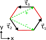
Figure 1: Schematics of the honeycomb lattice. Ferromagnetic order is assumed to be in the z − limit-from 𝑧 z- 𝝉 1 = 1 2 ( 1 3 , 1 ) subscript 𝝉 1 1 2 1 3 1 {\bm{\tau}}_{1}=\frac{1}{2}\left(\frac{1}{\sqrt{3}},1\right) 𝝉 2 = 1 2 ( 1 3 , − 1 ) subscript 𝝉 2 1 2 1 3 1 {\bm{\tau}}_{2}=\frac{1}{2}\left(\frac{1}{\sqrt{3}},-1\right) 𝝉 3 = 1 3 ( − 1 , 0 ) subscript 𝝉 3 1 3 1 0 {\bm{\tau}}_{3}=\frac{1}{\sqrt{3}}(-1,0) ν i j = ± 1 subscript 𝜈 𝑖 𝑗 plus-or-minus 1 \nu_{ij}=\pm 1
We study spins of the length S 𝑆 S z 𝑧 z ABP1967 ; Auerbach ; Rezende S ± = S x ± i S y superscript 𝑆 plus-or-minus plus-or-minus superscript 𝑆 𝑥 𝑖 superscript 𝑆 𝑦 S^{\pm}=S^{x}\pm iS^{y} S z superscript 𝑆 𝑧 S^{z}
S + = 2 S − a † a a , S − = a † 2 S − a † a , S z = S − a † a . formulae-sequence superscript 𝑆 2 𝑆 superscript 𝑎 † 𝑎 𝑎 formulae-sequence superscript 𝑆 superscript 𝑎 † 2 𝑆 superscript 𝑎 † 𝑎 superscript 𝑆 𝑧 𝑆 superscript 𝑎 † 𝑎 \displaystyle S^{+}=\sqrt{2S-a^{{\dagger}}a}a,~{}~{}~{}S^{-}=a^{{\dagger}}\sqrt{2S-a^{{\dagger}}a},~{}~{}~{}S^{z}=S-a^{{\dagger}}a. (1)
Exchange interaction is
H ex = − J ∑ ⟨ i j ⟩ ( S i x S j x + S i y S j y + S i z S j z ) = − J ∑ ⟨ i j ⟩ ( 1 2 S i + S j − + 1 2 S i − S j + + S i z S j z ) , subscript 𝐻 ex 𝐽 subscript delimited-⟨⟩ 𝑖 𝑗 subscript superscript 𝑆 𝑥 𝑖 subscript superscript 𝑆 𝑥 𝑗 subscript superscript 𝑆 𝑦 𝑖 subscript superscript 𝑆 𝑦 𝑗 subscript superscript 𝑆 𝑧 𝑖 subscript superscript 𝑆 𝑧 𝑗 𝐽 subscript delimited-⟨⟩ 𝑖 𝑗 1 2 subscript superscript 𝑆 𝑖 subscript superscript 𝑆 𝑗 1 2 subscript superscript 𝑆 𝑖 subscript superscript 𝑆 𝑗 subscript superscript 𝑆 𝑧 𝑖 subscript superscript 𝑆 𝑧 𝑗 \displaystyle H_{\mathrm{ex}}=-J\sum_{\langle ij\rangle}\left(S^{x}_{i}S^{x}_{j}+S^{y}_{i}S^{y}_{j}+S^{z}_{i}S^{z}_{j}\right)=-J\sum_{\langle ij\rangle}\left(\frac{1}{2}S^{+}_{i}S^{-}_{j}+\frac{1}{2}S^{-}_{i}S^{+}_{j}+S^{z}_{i}S^{z}_{j}\right), (2)
where ⟨ . . ⟩ \langle..\rangle S > 1 𝑆 1 S>1 1 S 1 𝑆 \frac{1}{S}
H sw = subscript 𝐻 sw absent \displaystyle H_{\mathrm{sw}}= − J S ∑ ⟨ i j ⟩ ( a i † b j + b j † a i ) + 3 J S ∑ ⟨ i j ⟩ ( a i † a i + b j † b j ) 𝐽 𝑆 subscript delimited-⟨⟩ 𝑖 𝑗 superscript subscript 𝑎 𝑖 † subscript 𝑏 𝑗 superscript subscript 𝑏 𝑗 † subscript 𝑎 𝑖 3 𝐽 𝑆 subscript delimited-⟨⟩ 𝑖 𝑗 superscript subscript 𝑎 𝑖 † subscript 𝑎 𝑖 superscript subscript 𝑏 𝑗 † subscript 𝑏 𝑗 \displaystyle-JS\sum_{\langle ij\rangle}\left(a_{i}^{{\dagger}}b_{j}+b_{j}^{{\dagger}}a_{i}\right)+3JS\sum_{\langle ij\rangle}\left(a_{i}^{{\dagger}}a_{i}+b_{j}^{{\dagger}}b_{j}\right) (3)
+ J 4 ∑ ⟨ i j ⟩ a i † a i a i b j † + J 4 ∑ ⟨ i j ⟩ a i b j † b j † b j + J 4 ∑ ⟨ i j ⟩ a i † a i † a i b j + J 4 ∑ ⟨ i j ⟩ a i † b j † b j b j − J ∑ ⟨ i j ⟩ a i † a i b j † b j . 𝐽 4 subscript delimited-⟨⟩ 𝑖 𝑗 superscript subscript 𝑎 𝑖 † subscript 𝑎 𝑖 subscript 𝑎 𝑖 superscript subscript 𝑏 𝑗 † 𝐽 4 subscript delimited-⟨⟩ 𝑖 𝑗 subscript 𝑎 𝑖 superscript subscript 𝑏 𝑗 † superscript subscript 𝑏 𝑗 † subscript 𝑏 𝑗 𝐽 4 subscript delimited-⟨⟩ 𝑖 𝑗 superscript subscript 𝑎 𝑖 † superscript subscript 𝑎 𝑖 † subscript 𝑎 𝑖 subscript 𝑏 𝑗 𝐽 4 subscript delimited-⟨⟩ 𝑖 𝑗 superscript subscript 𝑎 𝑖 † superscript subscript 𝑏 𝑗 † subscript 𝑏 𝑗 subscript 𝑏 𝑗 𝐽 subscript delimited-⟨⟩ 𝑖 𝑗 superscript subscript 𝑎 𝑖 † subscript 𝑎 𝑖 superscript subscript 𝑏 𝑗 † subscript 𝑏 𝑗 \displaystyle+\frac{J}{4}\sum_{\langle ij\rangle}a_{i}^{{\dagger}}a_{i}a_{i}b_{j}^{{\dagger}}+\frac{J}{4}\sum_{\langle ij\rangle}a_{i}b_{j}^{{\dagger}}b_{j}^{{\dagger}}b_{j}+\frac{J}{4}\sum_{\langle ij\rangle}a_{i}^{{\dagger}}a_{i}^{{\dagger}}a_{i}b_{j}+\frac{J}{4}\sum_{\langle ij\rangle}a_{i}^{{\dagger}}b_{j}^{{\dagger}}b_{j}b_{j}-J\sum_{\langle ij\rangle}a_{i}^{{\dagger}}a_{i}b_{j}^{{\dagger}}b_{j}. (4)
Fourier transform of the Hamiltonian reads as
H sw ≈ − J S ∫ 𝐤 ( γ 𝐤 a 𝐤 † b 𝐤 + γ 𝐤 ∗ b 𝐤 † a 𝐤 ) + 3 J S ∫ 𝐤 ( a 𝐤 † a 𝐤 + b 𝐤 † b 𝐤 ) − J ∫ { 𝐤 } δ 𝐤 1 − 𝐤 2 , 𝐤 4 − 𝐤 3 γ 𝐤 4 − 𝐤 3 a 𝐤 1 † b 𝐤 3 † a 𝐤 2 b 𝐤 4 subscript 𝐻 sw 𝐽 𝑆 subscript 𝐤 subscript 𝛾 𝐤 superscript subscript 𝑎 𝐤 † subscript 𝑏 𝐤 superscript subscript 𝛾 𝐤 superscript subscript 𝑏 𝐤 † subscript 𝑎 𝐤 3 𝐽 𝑆 subscript 𝐤 superscript subscript 𝑎 𝐤 † subscript 𝑎 𝐤 superscript subscript 𝑏 𝐤 † subscript 𝑏 𝐤 𝐽 subscript 𝐤 subscript 𝛿 subscript 𝐤 1 subscript 𝐤 2 subscript 𝐤 4 subscript 𝐤 3
subscript 𝛾 subscript 𝐤 4 subscript 𝐤 3 superscript subscript 𝑎 subscript 𝐤 1 † superscript subscript 𝑏 subscript 𝐤 3 † subscript 𝑎 subscript 𝐤 2 subscript 𝑏 subscript 𝐤 4 \displaystyle H_{\mathrm{sw}}\approx-JS\int_{\bf k}\left(\gamma_{{\bf k}}a_{{\bf k}}^{{\dagger}}b_{{\bf k}}+\gamma_{{\bf k}}^{*}b_{{\bf k}}^{{\dagger}}a_{{\bf k}}\right)+3JS\int_{\bf k}\left(a_{{\bf k}}^{{\dagger}}a_{{\bf k}}+b_{{\bf k}}^{{\dagger}}b_{{\bf k}}\right)-J\int_{\{{\bf k}\}}\delta_{{\bf k}_{1}-{\bf k}_{2},{\bf k}_{4}-{\bf k}_{3}}\gamma_{{\bf k}_{4}-{\bf k}_{3}}a_{{\bf k}_{1}}^{{\dagger}}b_{{\bf k}_{3}}^{{\dagger}}a_{{\bf k}_{2}}b_{{\bf k}_{4}} (5)
+ J 4 ∫ { 𝐤 } δ 𝐤 1 − 𝐤 2 , 𝐤 4 − 𝐤 3 [ γ 𝐤 3 ∗ a 𝐤 1 † b 𝐤 3 † a 𝐤 2 a 𝐤 4 + γ 𝐤 3 a 𝐤 2 † a 𝐤 4 † a 𝐤 1 b 𝐤 3 ] + J 4 ∫ { 𝐤 } δ 𝐤 1 − 𝐤 2 , 𝐤 4 − 𝐤 3 [ γ 𝐤 1 a 𝐤 1 † b 𝐤 3 † b 𝐤 2 b 𝐤 4 + γ 𝐤 1 ∗ b 𝐤 2 † b 𝐤 4 † a 𝐤 1 b 𝐤 3 ] , 𝐽 4 subscript 𝐤 subscript 𝛿 subscript 𝐤 1 subscript 𝐤 2 subscript 𝐤 4 subscript 𝐤 3
delimited-[] superscript subscript 𝛾 subscript 𝐤 3 superscript subscript 𝑎 subscript 𝐤 1 † superscript subscript 𝑏 subscript 𝐤 3 † subscript 𝑎 subscript 𝐤 2 subscript 𝑎 subscript 𝐤 4 subscript 𝛾 subscript 𝐤 3 superscript subscript 𝑎 subscript 𝐤 2 † superscript subscript 𝑎 subscript 𝐤 4 † subscript 𝑎 subscript 𝐤 1 subscript 𝑏 subscript 𝐤 3 𝐽 4 subscript 𝐤 subscript 𝛿 subscript 𝐤 1 subscript 𝐤 2 subscript 𝐤 4 subscript 𝐤 3
delimited-[] subscript 𝛾 subscript 𝐤 1 superscript subscript 𝑎 subscript 𝐤 1 † superscript subscript 𝑏 subscript 𝐤 3 † subscript 𝑏 subscript 𝐤 2 subscript 𝑏 subscript 𝐤 4 superscript subscript 𝛾 subscript 𝐤 1 superscript subscript 𝑏 subscript 𝐤 2 † superscript subscript 𝑏 subscript 𝐤 4 † subscript 𝑎 subscript 𝐤 1 subscript 𝑏 subscript 𝐤 3 \displaystyle+\frac{J}{4}\int_{\{{\bf k}\}}\delta_{{\bf k}_{1}-{\bf k}_{2},{\bf k}_{4}-{\bf k}_{3}}\left[\gamma_{{\bf k}_{3}}^{*}a_{{\bf k}_{1}}^{{\dagger}}b_{{\bf k}_{3}}^{{\dagger}}a_{{\bf k}_{2}}a_{{\bf k}_{4}}+\gamma_{{\bf k}_{3}}a_{{\bf k}_{2}}^{{\dagger}}a_{{\bf k}_{4}}^{{\dagger}}a_{{\bf k}_{1}}b_{{\bf k}_{3}}\right]+\frac{J}{4}\int_{\{{\bf k}\}}\delta_{{\bf k}_{1}-{\bf k}_{2},{\bf k}_{4}-{\bf k}_{3}}\left[\gamma_{{\bf k}_{1}}a_{{\bf k}_{1}}^{{\dagger}}b_{{\bf k}_{3}}^{{\dagger}}b_{{\bf k}_{2}}b_{{\bf k}_{4}}+\gamma_{{\bf k}_{1}}^{*}b_{{\bf k}_{2}}^{{\dagger}}b_{{\bf k}_{4}}^{{\dagger}}a_{{\bf k}_{1}}b_{{\bf k}_{3}}\right],
where γ 𝐤 = ∑ i = 1 , 2 , 3 e i 𝐤 𝝉 i = 2 e i k x 2 3 cos ( k y 2 ) + e − i k x 3 subscript 𝛾 𝐤 subscript 𝑖 1 2 3
superscript 𝑒 𝑖 𝐤 subscript 𝝉 𝑖 2 superscript 𝑒 𝑖 subscript 𝑘 𝑥 2 3 subscript 𝑘 𝑦 2 superscript 𝑒 𝑖 subscript 𝑘 𝑥 3 \gamma_{\bf k}=\sum_{i=1,2,3}e^{i{\bf k}{\bm{\tau}}_{i}}=2e^{i\frac{k_{x}}{2\sqrt{3}}}\cos\left(\frac{k_{y}}{2}\right)+e^{-i\frac{k_{x}}{\sqrt{3}}} 1 𝝉 i subscript 𝝉 𝑖 {\bm{\tau}}_{i} { 𝐤 } ≡ 𝐤 1 , 𝐤 2 , 𝐤 3 , 𝐤 4 𝐤 subscript 𝐤 1 subscript 𝐤 2 subscript 𝐤 3 subscript 𝐤 4
\{{\bf k}\}\equiv{\bf k}_{1},{\bf k}_{2},{\bf k}_{3},{\bf k}_{4} δ 𝐤 1 , 𝐤 2 ≡ 2 π δ ( 𝐤 1 − 𝐤 2 ) subscript 𝛿 subscript 𝐤 1 subscript 𝐤 2
2 𝜋 𝛿 subscript 𝐤 1 subscript 𝐤 2 \delta_{{\bf k}_{1},{\bf k}_{2}}\equiv 2\pi\delta({\bf k}_{1}-{\bf k}_{2})
− J ∫ { 𝐤 } δ 𝐤 1 − 𝐤 2 , 𝐤 4 − 𝐤 3 ∫ ϵ 1 , ϵ 2 , ϵ 3 , ϵ 4 a ϵ 1 ; 𝐤 1 † b ϵ 3 ; 𝐤 3 † a ϵ 2 ; 𝐤 2 b ϵ 4 ; 𝐤 4 δ ϵ 1 − ϵ 2 , ϵ 4 − ϵ 3 𝐽 subscript 𝐤 subscript 𝛿 subscript 𝐤 1 subscript 𝐤 2 subscript 𝐤 4 subscript 𝐤 3
subscript subscript italic-ϵ 1 subscript italic-ϵ 2 subscript italic-ϵ 3 subscript italic-ϵ 4
superscript subscript 𝑎 subscript italic-ϵ 1 subscript 𝐤 1
† superscript subscript 𝑏 subscript italic-ϵ 3 subscript 𝐤 3
† subscript 𝑎 subscript italic-ϵ 2 subscript 𝐤 2
subscript 𝑏 subscript italic-ϵ 4 subscript 𝐤 4
subscript 𝛿 subscript italic-ϵ 1 subscript italic-ϵ 2 subscript italic-ϵ 4 subscript italic-ϵ 3
\displaystyle-J\int_{\{{\bf k}\}}\delta_{{\bf k}_{1}-{\bf k}_{2},{\bf k}_{4}-{\bf k}_{3}}\int_{\epsilon_{1},\epsilon_{2},\epsilon_{3},\epsilon_{4}}a_{\epsilon_{1};{\bf k}_{1}}^{{\dagger}}b_{\epsilon_{3};{\bf k}_{3}}^{{\dagger}}a_{\epsilon_{2};{\bf k}_{2}}b_{\epsilon_{4};{\bf k}_{4}}\delta_{\epsilon_{1}-\epsilon_{2},\epsilon_{4}-\epsilon_{3}} (6)
= \displaystyle= − J ∫ { 𝐤 } δ 𝐤 1 − 𝐤 2 , 𝐤 4 − 𝐤 3 ∫ ϵ 1 , ϵ 3 , ω a ϵ 1 ; 𝐤 1 † b ϵ 3 ; 𝐤 3 † a ϵ 1 − ω ; 𝐤 2 b ϵ 3 + ω ; 𝐤 4 . 𝐽 subscript 𝐤 subscript 𝛿 subscript 𝐤 1 subscript 𝐤 2 subscript 𝐤 4 subscript 𝐤 3
subscript subscript italic-ϵ 1 subscript italic-ϵ 3 𝜔
superscript subscript 𝑎 subscript italic-ϵ 1 subscript 𝐤 1
† superscript subscript 𝑏 subscript italic-ϵ 3 subscript 𝐤 3
† subscript 𝑎 subscript italic-ϵ 1 𝜔 subscript 𝐤 2
subscript 𝑏 subscript italic-ϵ 3 𝜔 subscript 𝐤 4
\displaystyle-J\int_{\{{\bf k}\}}\delta_{{\bf k}_{1}-{\bf k}_{2},{\bf k}_{4}-{\bf k}_{3}}\int_{\epsilon_{1},\epsilon_{3},\omega}a_{\epsilon_{1};{\bf k}_{1}}^{{\dagger}}b_{\epsilon_{3};{\bf k}_{3}}^{{\dagger}}a_{\epsilon_{1}-\omega;{\bf k}_{2}}b_{\epsilon_{3}+\omega;{\bf k}_{4}}. (7)
In the space of unitary cell, in which case the boson operators are defined by Ψ 𝐤 † = ( a 𝐤 † , b 𝐤 † ) superscript subscript Ψ 𝐤 † superscript subscript 𝑎 𝐤 † superscript subscript 𝑏 𝐤 † \Psi_{\bf k}^{\dagger}=(a_{\bf k}^{{\dagger}},~{}b_{\bf k}^{{\dagger}})
H ^ = J S [ 3 − γ 𝐤 − γ 𝐤 ∗ 3 ] , ^ 𝐻 𝐽 𝑆 delimited-[] 3 subscript 𝛾 𝐤 superscript subscript 𝛾 𝐤 3 \displaystyle\hat{H}=JS\left[\begin{array}[]{cc}3&-\gamma_{\bf k}\\
-\gamma_{\bf k}^{*}&3\end{array}\right], (10)
diagonalization immediatly gives energy spectrum,
ϵ ± 𝐤 = J S ( 3 ± | γ 𝐤 | ) subscript italic-ϵ plus-or-minus 𝐤 𝐽 𝑆 plus-or-minus 3 subscript 𝛾 𝐤 \displaystyle\epsilon_{\pm{\bf k}}=JS\left(3\pm|\gamma_{\bf k}|\right) (11)
with corresponding wave functions
φ + = 1 2 [ − γ 𝐤 | γ 𝐤 | 1 ] , φ − = 1 2 [ γ 𝐤 | γ 𝐤 | 1 ] , formulae-sequence subscript 𝜑 1 2 delimited-[] subscript 𝛾 𝐤 subscript 𝛾 𝐤 1 subscript 𝜑 1 2 delimited-[] subscript 𝛾 𝐤 subscript 𝛾 𝐤 1 \displaystyle\varphi_{+}=\frac{1}{\sqrt{2}}\left[\begin{array}[]{c}-\frac{\gamma_{\bf k}}{|\gamma_{\bf k}|}\\
1\end{array}\right],~{}~{}~{}\varphi_{-}=\frac{1}{\sqrt{2}}\left[\begin{array}[]{c}\frac{\gamma_{\bf k}}{|\gamma_{\bf k}|}\\
1\end{array}\right], (16)
Green function is
G α β R / A ( ϵ , 𝐤 ) = φ + , 𝐤 φ + , 𝐤 † ϵ − ϵ + , 𝐤 ± i 0 + φ − , 𝐤 φ − , 𝐤 † ϵ − ϵ − , 𝐤 ± i 0 , superscript subscript 𝐺 𝛼 𝛽 R A italic-ϵ 𝐤 subscript 𝜑 𝐤
subscript superscript 𝜑 † 𝐤
plus-or-minus italic-ϵ subscript italic-ϵ 𝐤
𝑖 0 subscript 𝜑 𝐤
subscript superscript 𝜑 † 𝐤
plus-or-minus italic-ϵ subscript italic-ϵ 𝐤
𝑖 0 \displaystyle G_{\alpha\beta}^{\mathrm{R}/\mathrm{A}}(\epsilon,{\bf k})=\frac{\varphi_{+,{\bf k}}\varphi^{{\dagger}}_{+,{\bf k}}}{\epsilon-\epsilon_{+,{\bf k}}\pm i0}+\frac{\varphi_{-,{\bf k}}\varphi^{{\dagger}}_{-,{\bf k}}}{\epsilon-\epsilon_{-,{\bf k}}\pm i0}, (17)
where α 𝛼 \alpha β 𝛽 \beta
G α β R / A ( ϵ , 𝐤 ) = superscript subscript 𝐺 𝛼 𝛽 R A italic-ϵ 𝐤 absent \displaystyle G_{\alpha\beta}^{\mathrm{R}/\mathrm{A}}(\epsilon,{\bf k})= 1 2 ( 1 ϵ − ϵ + , 𝐤 ± i 0 + 1 ϵ − ϵ − , 𝐤 ± i 0 ) − 1 2 ( 1 ϵ − ϵ + , 𝐤 ± i 0 − 1 ϵ − ϵ − , 𝐤 ± i 0 ) [ 0 γ 𝐤 | γ 𝐤 | γ 𝐤 ∗ | γ 𝐤 | 0 ] . 1 2 1 plus-or-minus italic-ϵ subscript italic-ϵ 𝐤
𝑖 0 1 plus-or-minus italic-ϵ subscript italic-ϵ 𝐤
𝑖 0 1 2 1 plus-or-minus italic-ϵ subscript italic-ϵ 𝐤
𝑖 0 1 plus-or-minus italic-ϵ subscript italic-ϵ 𝐤
𝑖 0 delimited-[] 0 subscript 𝛾 𝐤 subscript 𝛾 𝐤 superscript subscript 𝛾 𝐤 subscript 𝛾 𝐤 0 \displaystyle\frac{1}{2}\left(\frac{1}{\epsilon-\epsilon_{+,{\bf k}}\pm i0}+\frac{1}{\epsilon-\epsilon_{-,{\bf k}}\pm i0}\right)-\frac{1}{2}\left(\frac{1}{\epsilon-\epsilon_{+,{\bf k}}\pm i0}-\frac{1}{\epsilon-\epsilon_{-,{\bf k}}\pm i0}\right)\left[\begin{array}[]{cc}0&\frac{\gamma_{\bf k}}{|\gamma_{\bf k}|}\\
\frac{\gamma_{\bf k}^{*}}{|\gamma_{\bf k}|}&0\end{array}\right]. (20)
The pumping is
H pump subscript 𝐻 pump \displaystyle H_{\mathrm{pump}} = Γ ∑ i [ S i x cos ( Ω t ) + S i y sin ( Ω t ) ] = Γ 2 ∑ i [ S i + e − i Ω t + S i − e i Ω t ] absent Γ subscript 𝑖 delimited-[] subscript superscript 𝑆 𝑥 𝑖 Ω 𝑡 subscript superscript 𝑆 𝑦 𝑖 Ω 𝑡 Γ 2 subscript 𝑖 delimited-[] subscript superscript 𝑆 𝑖 superscript 𝑒 𝑖 Ω 𝑡 subscript superscript 𝑆 𝑖 superscript 𝑒 𝑖 Ω 𝑡 \displaystyle=\Gamma\sum_{i}\left[S^{x}_{i}\cos(\Omega t)+S^{y}_{i}\sin(\Omega t)\right]=\frac{\Gamma}{2}\sum_{i}\left[S^{+}_{i}e^{-i\Omega t}+S^{-}_{i}e^{i\Omega t}\right] (21)
≈ 2 S Γ 2 ∑ i [ a i e − i Ω t + a i † e i Ω t ] + 2 S Γ 2 ∑ i [ b i e − i Ω t + b i † e i Ω t ] . absent 2 𝑆 Γ 2 subscript 𝑖 delimited-[] subscript 𝑎 𝑖 superscript 𝑒 𝑖 Ω 𝑡 subscript superscript 𝑎 † 𝑖 superscript 𝑒 𝑖 Ω 𝑡 2 𝑆 Γ 2 subscript 𝑖 delimited-[] subscript 𝑏 𝑖 superscript 𝑒 𝑖 Ω 𝑡 subscript superscript 𝑏 † 𝑖 superscript 𝑒 𝑖 Ω 𝑡 \displaystyle\approx\sqrt{2S}\frac{\Gamma}{2}\sum_{i}\left[a_{i}e^{-i\Omega t}+a^{{\dagger}}_{i}e^{i\Omega t}\right]+\sqrt{2S}\frac{\Gamma}{2}\sum_{i}\left[b_{i}e^{-i\Omega t}+b^{{\dagger}}_{i}e^{i\Omega t}\right]. (22)
For the sake of discussion, we also consider Dzyaloshinskii-Moriya interaction
H DMI = D ∑ ⟨ ⟨ i j ⟩ ⟩ ν i j [ 𝐒 i × 𝐒 j ] z , subscript 𝐻 DMI 𝐷 subscript delimited-⟨⟩ delimited-⟨⟩ 𝑖 𝑗 subscript 𝜈 𝑖 𝑗 subscript delimited-[] subscript 𝐒 𝑖 subscript 𝐒 𝑗 𝑧 \displaystyle H_{\mathrm{DMI}}=D\sum_{\langle\langle ij\rangle\rangle}\nu_{ij}[{\bf S}_{i}\times{\bf S}_{j}]_{z}, (23)
where ⟨ ⟨ i j ⟩ ⟩ delimited-⟨⟩ delimited-⟨⟩ 𝑖 𝑗 \langle\langle ij\rangle\rangle ν i j = ± 1 subscript 𝜈 𝑖 𝑗 plus-or-minus 1 \nu_{ij}=\pm 1 1
H DMI = S D ∫ 𝐤 ξ 𝐤 ( a 𝐤 † a 𝐤 − b 𝐤 † b 𝐤 ) , subscript 𝐻 DMI 𝑆 𝐷 subscript 𝐤 subscript 𝜉 𝐤 subscript superscript 𝑎 † 𝐤 subscript 𝑎 𝐤 subscript superscript 𝑏 † 𝐤 subscript 𝑏 𝐤 \displaystyle H_{\mathrm{DMI}}=SD\int_{\bf k}\xi_{\bf k}\left(a^{{\dagger}}_{\bf k}a_{\bf k}-b^{{\dagger}}_{\bf k}b_{\bf k}\right), (24)
where ξ 𝐤 = 2 [ sin ( k y ) − 2 sin ( k y 2 ) cos ( 3 k x 2 ) ] subscript 𝜉 𝐤 2 delimited-[] subscript 𝑘 𝑦 2 subscript 𝑘 𝑦 2 3 subscript 𝑘 𝑥 2 \xi_{\bf k}=2\left[\sin(k_{y})-2\sin\left(\frac{k_{y}}{2}\right)\cos\left(\frac{\sqrt{3}k_{x}}{2}\right)\right]
III Keldysh formalism
We stress that in the hindsight, the Keldysh technique is certainly not the only choice for the problem at hand. It seems that Matsubara frequency space should work equally well. However, as the system under study is pumped and formally out-of-equilibrium, we decided to be on a safe side and follow non-equilibrium field theory technique - the Keldysh technique.
Here we briefly outline steps of the Keldysh technique, which we utilized in analysis of the system.
For a detailed review of the Keldysh formalism see book Kamenev Ψ ¯ + , Ψ + superscript ¯ Ψ superscript Ψ
\bar{\Psi}^{+},\Psi^{+} Ψ ¯ − , Ψ − superscript ¯ Ψ superscript Ψ
\bar{\Psi}^{-},\Psi^{-}
∫ 𝒞 𝑑 t Ψ ¯ ( t ) H ^ Ψ ( t ) = ∫ − ∞ + ∞ 𝑑 t Ψ ¯ + ( t ) H ^ Ψ + ( t ) − ∫ − ∞ + ∞ 𝑑 t Ψ ¯ − ( t ) H ^ Ψ − ( t ) = ∫ − ∞ + ∞ 𝑑 t [ Ψ ¯ cl ( t ) H ^ Ψ q ( t ) + Ψ ¯ q ( t ) H ^ Ψ cl ( t ) ] , subscript 𝒞 differential-d 𝑡 ¯ Ψ 𝑡 ^ 𝐻 Ψ 𝑡 superscript subscript differential-d 𝑡 superscript ¯ Ψ 𝑡 ^ 𝐻 superscript Ψ 𝑡 superscript subscript differential-d 𝑡 superscript ¯ Ψ 𝑡 ^ 𝐻 superscript Ψ 𝑡 superscript subscript differential-d 𝑡 delimited-[] superscript ¯ Ψ cl 𝑡 ^ 𝐻 superscript Ψ q 𝑡 superscript ¯ Ψ q 𝑡 ^ 𝐻 superscript Ψ cl 𝑡 \displaystyle\int_{{\cal C}}dt\bar{\Psi}(t)\hat{H}\Psi(t)=\int_{-\infty}^{+\infty}dt\bar{\Psi}^{+}(t)\hat{H}\Psi^{+}(t)-\int_{-\infty}^{+\infty}dt\bar{\Psi}^{-}(t)\hat{H}\Psi^{-}(t)=\int_{-\infty}^{+\infty}dt\left[\bar{\Psi}^{\mathrm{cl}}(t)\hat{H}\Psi^{\mathrm{q}}(t)+\bar{\Psi}^{\mathrm{q}}(t)\hat{H}\Psi^{\mathrm{cl}}(t)\right], (25)
where
Ψ cl / q = 1 2 ( Ψ + ± Ψ − ) , superscript Ψ cl q 1 2 plus-or-minus superscript Ψ superscript Ψ \displaystyle\Psi^{\mathrm{cl}/\mathrm{q}}=\frac{1}{\sqrt{2}}\left(\Psi^{+}\pm\Psi^{-}\right), (26)
and the same for Ψ ¯ ¯ Ψ \bar{\Psi}
i S = i ∫ − ∞ + ∞ 𝑑 t Ψ ¯ ( t ) [ 0 [ G − 1 ] A [ G − 1 ] R [ G − 1 ] K ] Ψ ( t ) 𝑖 𝑆 𝑖 superscript subscript differential-d 𝑡 ¯ Ψ 𝑡 delimited-[] 0 superscript delimited-[] superscript 𝐺 1 A superscript delimited-[] superscript 𝐺 1 R superscript delimited-[] superscript 𝐺 1 K Ψ 𝑡 \displaystyle iS=i\int_{-\infty}^{+\infty}dt\bar{\Psi}(t)\left[\begin{array}[]{cc}0&\left[G^{-1}\right]^{\mathrm{A}}\\
\left[G^{-1}\right]^{\mathrm{R}}&\left[G^{-1}\right]^{\mathrm{K}}\end{array}\right]\Psi(t) (29)
where
Ψ = [ Ψ cl Ψ q ] , Ψ ¯ = [ Ψ ¯ cl Ψ ¯ q ] , formulae-sequence Ψ delimited-[] superscript Ψ cl superscript Ψ q ¯ Ψ delimited-[] superscript ¯ Ψ cl superscript ¯ Ψ q \displaystyle\Psi=\left[\begin{array}[]{c}\Psi^{\mathrm{cl}}\\
\Psi^{\mathrm{q}}\end{array}\right],~{}~{}~{}~{}\bar{\Psi}=\left[\begin{array}[]{cc}\bar{\Psi}^{\mathrm{cl}}&\bar{\Psi}^{\mathrm{q}}\end{array}\right], (33)
and [ G − 1 ( ϵ ) ] R / A = ϵ ± i 0 − H ^ superscript delimited-[] superscript 𝐺 1 italic-ϵ R A plus-or-minus italic-ϵ 𝑖 0 ^ 𝐻 \left[G^{-1}(\epsilon)\right]^{\mathrm{R}/\mathrm{A}}=\epsilon\pm i0-\hat{H} [ G − 1 ] K superscript delimited-[] superscript 𝐺 1 K [G^{-1}]^{\mathrm{K}}
⟨ Ψ ( t ) Ψ ¯ ( t ′ ) ⟩ S = i [ G K ( t − t ′ ) G R ( t − t ′ ) G A ( t − t ′ ) 0 ] , subscript delimited-⟨⟩ Ψ 𝑡 ¯ Ψ superscript 𝑡 ′ 𝑆 𝑖 delimited-[] superscript 𝐺 K 𝑡 superscript 𝑡 ′ superscript 𝐺 R 𝑡 superscript 𝑡 ′ superscript 𝐺 A 𝑡 superscript 𝑡 ′ 0 \displaystyle\langle\Psi(t)\bar{\Psi}(t^{\prime})\rangle_{S}=i\left[\begin{array}[]{cc}G^{\mathrm{K}}(t-t^{\prime})&G^{\mathrm{R}}(t-t^{\prime})\\
G^{\mathrm{A}}(t-t^{\prime})&0\end{array}\right], (36)
where in particular
⟨ Ψ cl ( t ) Ψ ¯ cl ( t ′ ) ⟩ S = ∑ ϵ i G K ( ϵ ) e − i ϵ ( t − t ′ ) , subscript delimited-⟨⟩ superscript Ψ cl 𝑡 superscript ¯ Ψ cl superscript 𝑡 ′ 𝑆 subscript italic-ϵ 𝑖 superscript 𝐺 K italic-ϵ superscript 𝑒 𝑖 italic-ϵ 𝑡 superscript 𝑡 ′ \displaystyle\langle\Psi^{\mathrm{cl}}(t)\bar{\Psi}^{\mathrm{cl}}(t^{\prime})\rangle_{S}=\sum_{\epsilon}iG^{\mathrm{K}}(\epsilon)e^{-i\epsilon(t-t^{\prime})}, (37)
⟨ Ψ cl ( t ) Ψ ¯ q ( t ′ ) ⟩ S = ∑ ϵ i G R ( ϵ ) e − i ϵ ( t − t ′ ) , subscript delimited-⟨⟩ superscript Ψ cl 𝑡 superscript ¯ Ψ q superscript 𝑡 ′ 𝑆 subscript italic-ϵ 𝑖 superscript 𝐺 R italic-ϵ superscript 𝑒 𝑖 italic-ϵ 𝑡 superscript 𝑡 ′ \displaystyle\langle\Psi^{\mathrm{cl}}(t)\bar{\Psi}^{\mathrm{q}}(t^{\prime})\rangle_{S}=\sum_{\epsilon}iG^{\mathrm{R}}(\epsilon)e^{-i\epsilon(t-t^{\prime})}, (38)
⟨ Ψ q ( t ) Ψ ¯ cl ( t ′ ) ⟩ S = ∑ ϵ i G A ( ϵ ) e − i ϵ ( t − t ′ ) . subscript delimited-⟨⟩ superscript Ψ q 𝑡 superscript ¯ Ψ cl superscript 𝑡 ′ 𝑆 subscript italic-ϵ 𝑖 superscript 𝐺 A italic-ϵ superscript 𝑒 𝑖 italic-ϵ 𝑡 superscript 𝑡 ′ \displaystyle\langle\Psi^{\mathrm{q}}(t)\bar{\Psi}^{\mathrm{cl}}(t^{\prime})\rangle_{S}=\sum_{\epsilon}iG^{\mathrm{A}}(\epsilon)e^{-i\epsilon(t-t^{\prime})}. (39)
In frequency space
⟨ Ψ cl ( ϵ 1 ) Ψ ¯ cl ( ϵ 2 ) ⟩ S = i G K ( ϵ 1 ) δ ϵ 1 , ϵ 2 , subscript delimited-⟨⟩ superscript Ψ cl subscript italic-ϵ 1 superscript ¯ Ψ cl subscript italic-ϵ 2 𝑆 𝑖 superscript 𝐺 K subscript italic-ϵ 1 subscript 𝛿 subscript italic-ϵ 1 subscript italic-ϵ 2
\displaystyle\langle\Psi^{\mathrm{cl}}(\epsilon_{1})\bar{\Psi}^{\mathrm{cl}}(\epsilon_{2})\rangle_{S}=iG^{\mathrm{K}}(\epsilon_{1})\delta_{\epsilon_{1},\epsilon_{2}}, (40)
⟨ Ψ cl ( ϵ 1 ) Ψ ¯ q ( ϵ 2 ) ⟩ S = i G R ( ϵ 1 ) δ ϵ 1 , ϵ 2 , subscript delimited-⟨⟩ superscript Ψ cl subscript italic-ϵ 1 superscript ¯ Ψ q subscript italic-ϵ 2 𝑆 𝑖 superscript 𝐺 R subscript italic-ϵ 1 subscript 𝛿 subscript italic-ϵ 1 subscript italic-ϵ 2
\displaystyle\langle\Psi^{\mathrm{cl}}(\epsilon_{1})\bar{\Psi}^{\mathrm{q}}(\epsilon_{2})\rangle_{S}=iG^{\mathrm{R}}(\epsilon_{1})\delta_{\epsilon_{1},\epsilon_{2}}, (41)
⟨ Ψ q ( ϵ 1 ) Ψ ¯ cl ( ϵ 2 ) ⟩ S = i G A ( ϵ 1 ) δ ϵ 1 , ϵ 2 , subscript delimited-⟨⟩ superscript Ψ q subscript italic-ϵ 1 superscript ¯ Ψ cl subscript italic-ϵ 2 𝑆 𝑖 superscript 𝐺 A subscript italic-ϵ 1 subscript 𝛿 subscript italic-ϵ 1 subscript italic-ϵ 2
\displaystyle\langle\Psi^{\mathrm{q}}(\epsilon_{1})\bar{\Psi}^{\mathrm{cl}}(\epsilon_{2})\rangle_{S}=iG^{\mathrm{A}}(\epsilon_{1})\delta_{\epsilon_{1},\epsilon_{2}}, (42)
where δ ϵ 1 , ϵ 2 = 2 π δ ( ϵ 1 − ϵ 2 ) subscript 𝛿 subscript italic-ϵ 1 subscript italic-ϵ 2
2 𝜋 𝛿 subscript italic-ϵ 1 subscript italic-ϵ 2 \delta_{\epsilon_{1},\epsilon_{2}}=2\pi\delta(\epsilon_{1}-\epsilon_{2})
[ 0 [ G − 1 ] A [ G − 1 ] R [ G − 1 ] K ] [ G K G R G A 0 ] = 1 , delimited-[] 0 superscript delimited-[] superscript 𝐺 1 A superscript delimited-[] superscript 𝐺 1 R superscript delimited-[] superscript 𝐺 1 K delimited-[] superscript 𝐺 K superscript 𝐺 R superscript 𝐺 A 0 1 \displaystyle\left[\begin{array}[]{cc}0&\left[G^{-1}\right]^{\mathrm{A}}\\
\left[G^{-1}\right]^{\mathrm{R}}&\left[G^{-1}\right]^{\mathrm{K}}\end{array}\right]\left[\begin{array}[]{cc}G^{\mathrm{K}}&G^{\mathrm{R}}\\
G^{\mathrm{A}}&0\end{array}\right]=1, (47)
which gives us a condition on G K superscript 𝐺 K G^{\mathrm{K}}
[ G − 1 ] R G K + [ G − 1 ] K G A = 0 , superscript delimited-[] superscript 𝐺 1 R superscript 𝐺 K superscript delimited-[] superscript 𝐺 1 K superscript 𝐺 A 0 \displaystyle\left[G^{-1}\right]^{\mathrm{R}}G^{\mathrm{K}}+\left[G^{-1}\right]^{\mathrm{K}}G^{\mathrm{A}}=0, (48)
which means
[ G − 1 ] K = − [ G − 1 ] R G K [ G − 1 ] A . superscript delimited-[] superscript 𝐺 1 K superscript delimited-[] superscript 𝐺 1 R superscript 𝐺 K superscript delimited-[] superscript 𝐺 1 A \displaystyle\left[G^{-1}\right]^{\mathrm{K}}=-\left[G^{-1}\right]^{\mathrm{R}}G^{\mathrm{K}}\left[G^{-1}\right]^{\mathrm{A}}. (49)
With the parametrization
G K = G R ℱ − ℱ G A , superscript 𝐺 K superscript 𝐺 R ℱ ℱ superscript 𝐺 A \displaystyle G^{\mathrm{K}}=G^{\mathrm{R}}{\cal F}-{\cal F}G^{\mathrm{A}}, (50)
where ℱ ℱ {\cal F}
[ G − 1 ] K = [ G − 1 ] R ℱ − ℱ [ G − 1 ] A . superscript delimited-[] superscript 𝐺 1 K superscript delimited-[] superscript 𝐺 1 R ℱ ℱ superscript delimited-[] superscript 𝐺 1 A \displaystyle\left[G^{-1}\right]^{\mathrm{K}}=\left[G^{-1}\right]^{\mathrm{R}}{\cal F}-{\cal F}\left[G^{-1}\right]^{\mathrm{A}}. (51)
This is the kinetic equation determining distribution function.
The pumping field is described by
2 S Γ 2 ∫ 𝒞 𝑑 t ( Ψ e − i Ω t + Ψ ¯ e i Ω t ) = Γ S ∫ − ∞ + ∞ 𝑑 t ( Ψ q e − i Ω t + Ψ ¯ q e i Ω t ) . 2 𝑆 Γ 2 subscript 𝒞 differential-d 𝑡 Ψ superscript 𝑒 𝑖 Ω 𝑡 ¯ Ψ superscript 𝑒 𝑖 Ω 𝑡 Γ 𝑆 superscript subscript differential-d 𝑡 superscript Ψ q superscript 𝑒 𝑖 Ω 𝑡 superscript ¯ Ψ q superscript 𝑒 𝑖 Ω 𝑡 \displaystyle\frac{\sqrt{2S}\Gamma}{2}\int_{\cal C}dt\left(\Psi e^{-i\Omega t}+\bar{\Psi}e^{i\Omega t}\right)=\Gamma\sqrt{S}\int_{-\infty}^{+\infty}dt\left(\Psi^{\mathrm{q}}e^{-i\Omega t}+\bar{\Psi}^{\mathrm{q}}e^{i\Omega t}\right). (52)
This might update the Hamiltonian and the Green functions.
To check this, we can use the following identity,
∫ d [ Ψ ¯ , Ψ ] e − ∑ i j Ψ ¯ i A ^ i j Ψ j + ∑ i ( Ψ ¯ i J i + J ¯ i Ψ i ) = 1 det A ^ e ∑ i j J ¯ i ( A ^ − 1 ) i j J j 𝑑 ¯ Ψ Ψ superscript 𝑒 subscript 𝑖 𝑗 subscript ¯ Ψ 𝑖 subscript ^ 𝐴 𝑖 𝑗 subscript Ψ 𝑗 subscript 𝑖 subscript ¯ Ψ 𝑖 subscript 𝐽 𝑖 subscript ¯ 𝐽 𝑖 subscript Ψ 𝑖 1 det ^ 𝐴 superscript 𝑒 subscript 𝑖 𝑗 subscript ¯ 𝐽 𝑖 subscript superscript ^ 𝐴 1 𝑖 𝑗 subscript 𝐽 𝑗 \displaystyle\int d[\bar{\Psi},\Psi]e^{-\sum_{ij}\bar{\Psi}_{i}\hat{A}_{ij}\Psi_{j}+\sum_{i}\left(\bar{\Psi}_{i}J_{i}+\bar{J}_{i}\Psi_{i}\right)}=\frac{1}{\mathrm{det}\hat{A}}e^{\sum_{ij}\bar{J}_{i}(\hat{A}^{-1})_{ij}J_{j}} (53)
and since there is no q q \mathrm{q} q q \mathrm{q} A ^ − 1 superscript ^ 𝐴 1 \hat{A}^{-1}
Now let us include interactions between magnons.
Schematically, general four-boson interaction rewritten in terms of Keldysh fields is
∫ 𝒞 𝑑 t Ψ ¯ 1 Ψ 2 Ψ ¯ 3 Ψ 4 subscript 𝒞 differential-d 𝑡 subscript ¯ Ψ 1 subscript Ψ 2 subscript ¯ Ψ 3 subscript Ψ 4 \displaystyle\int_{{\cal C}}dt\bar{\Psi}_{1}\Psi_{2}\bar{\Psi}_{3}\Psi_{4} = ∫ − ∞ + ∞ 𝑑 t Ψ ¯ 1 + Ψ 2 + Ψ ¯ 3 + Ψ 4 + − ∫ − ∞ + ∞ 𝑑 t Ψ ¯ 1 − Ψ 2 − Ψ ¯ 3 − Ψ 4 − absent superscript subscript differential-d 𝑡 superscript subscript ¯ Ψ 1 superscript subscript Ψ 2 superscript subscript ¯ Ψ 3 superscript subscript Ψ 4 superscript subscript differential-d 𝑡 superscript subscript ¯ Ψ 1 superscript subscript Ψ 2 superscript subscript ¯ Ψ 3 superscript subscript Ψ 4 \displaystyle=\int_{-\infty}^{+\infty}dt\bar{\Psi}_{1}^{+}\Psi_{2}^{+}\bar{\Psi}_{3}^{+}\Psi_{4}^{+}-\int_{-\infty}^{+\infty}dt\bar{\Psi}_{1}^{-}\Psi_{2}^{-}\bar{\Psi}_{3}^{-}\Psi_{4}^{-} (54)
= 1 2 ∫ − ∞ + ∞ 𝑑 t ( Ψ ¯ 1 cl Ψ 2 cl + Ψ ¯ 1 q Ψ 2 q ) ( Ψ ¯ 3 cl Ψ 4 q + Ψ ¯ 3 q Ψ 4 cl ) absent 1 2 superscript subscript differential-d 𝑡 superscript subscript ¯ Ψ 1 cl superscript subscript Ψ 2 cl superscript subscript ¯ Ψ 1 q superscript subscript Ψ 2 q superscript subscript ¯ Ψ 3 cl superscript subscript Ψ 4 q superscript subscript ¯ Ψ 3 q superscript subscript Ψ 4 cl \displaystyle=\frac{1}{2}\int_{-\infty}^{+\infty}dt\left(\bar{\Psi}_{1}^{\mathrm{cl}}\Psi_{2}^{\mathrm{cl}}+\bar{\Psi}_{1}^{\mathrm{q}}\Psi_{2}^{\mathrm{q}}\right)\left(\bar{\Psi}_{3}^{\mathrm{cl}}\Psi_{4}^{\mathrm{q}}+\bar{\Psi}_{3}^{\mathrm{q}}\Psi_{4}^{\mathrm{cl}}\right) (55)
+ 1 2 ∫ − ∞ + ∞ 𝑑 t ( Ψ ¯ 1 cl Ψ 2 q + Ψ ¯ 1 q Ψ 2 cl ) ( Ψ ¯ 3 cl Ψ 4 cl + Ψ ¯ 3 q Ψ 4 q ) 1 2 superscript subscript differential-d 𝑡 superscript subscript ¯ Ψ 1 cl superscript subscript Ψ 2 q superscript subscript ¯ Ψ 1 q superscript subscript Ψ 2 cl superscript subscript ¯ Ψ 3 cl superscript subscript Ψ 4 cl superscript subscript ¯ Ψ 3 q superscript subscript Ψ 4 q \displaystyle+\frac{1}{2}\int_{-\infty}^{+\infty}dt\left(\bar{\Psi}_{1}^{\mathrm{cl}}\Psi_{2}^{\mathrm{q}}+\bar{\Psi}_{1}^{\mathrm{q}}\Psi_{2}^{\mathrm{cl}}\right)\left(\bar{\Psi}_{3}^{\mathrm{cl}}\Psi_{4}^{\mathrm{cl}}+\bar{\Psi}_{3}^{\mathrm{q}}\Psi_{4}^{\mathrm{q}}\right) (56)
where 1 , 2 , 3 , 4 1 2 3 4
1,2,3,4
III.1 Shifting the pump field away
Lagrangian describing non-interacting magnons with the pump’s frequency Ω Ω \Omega 𝐤 = 0 𝐤 0 {\bf k}=0
ℒ 0 , Ω subscript ℒ 0 Ω
\displaystyle{\cal L}_{0,\Omega} = ∑ m , n Ψ ¯ m , 0 , Ω q ℒ ^ m n , 0 , Ω K Ψ n , 0 , Ω q + ∑ m , n Ψ ¯ m , 0 , Ω cl ℒ ^ m n , 0 , Ω A Ψ n , 0 , Ω q + ∑ m , n Ψ ¯ m , 0 , Ω q ℒ ^ m n , 0 , Ω R Ψ n , 0 , Ω cl absent subscript 𝑚 𝑛
subscript superscript ¯ Ψ q 𝑚 0 Ω
subscript superscript ^ ℒ K 𝑚 𝑛 0 Ω
subscript superscript Ψ q 𝑛 0 Ω
subscript 𝑚 𝑛
subscript superscript ¯ Ψ cl 𝑚 0 Ω
subscript superscript ^ ℒ A 𝑚 𝑛 0 Ω
subscript superscript Ψ q 𝑛 0 Ω
subscript 𝑚 𝑛
subscript superscript ¯ Ψ q 𝑚 0 Ω
subscript superscript ^ ℒ R 𝑚 𝑛 0 Ω
subscript superscript Ψ cl 𝑛 0 Ω
\displaystyle=\sum_{m,n}\bar{\Psi}^{\mathrm{q}}_{m,0,\Omega}\hat{{\cal L}}^{\mathrm{K}}_{mn,0,\Omega}\Psi^{\mathrm{q}}_{n,0,\Omega}+\sum_{m,n}\bar{\Psi}^{\mathrm{cl}}_{m,0,\Omega}\hat{{\cal L}}^{\mathrm{A}}_{mn,0,\Omega}\Psi^{\mathrm{q}}_{n,0,\Omega}+\sum_{m,n}\bar{\Psi}^{\mathrm{q}}_{m,0,\Omega}\hat{{\cal L}}^{\mathrm{R}}_{mn,0,\Omega}\Psi^{\mathrm{cl}}_{n,0,\Omega} (57)
− Γ S ∑ n Ψ n , 0 , Ω q − Γ S ∑ n Ψ ¯ n , 0 , Ω q , Γ 𝑆 subscript 𝑛 subscript superscript Ψ q 𝑛 0 Ω
Γ 𝑆 subscript 𝑛 subscript superscript ¯ Ψ q 𝑛 0 Ω
\displaystyle-\Gamma\sqrt{S}\sum_{n}\Psi^{\mathrm{q}}_{n,0,\Omega}-\Gamma\sqrt{S}\sum_{n}\bar{\Psi}^{\mathrm{q}}_{n,0,\Omega}, (58)
where ℒ ^ m n , 0 , Ω K / R / A subscript superscript ^ ℒ K R A 𝑚 𝑛 0 Ω
\hat{{\cal L}}^{\mathrm{K}/\mathrm{R}/\mathrm{A}}_{mn,0,\Omega} ℒ ^ m n , 𝐤 , Ω R / A = ( Ω ± i 0 ) δ m n − [ H ^ 0 ] m n , 𝐤 subscript superscript ^ ℒ R A 𝑚 𝑛 𝐤 Ω
plus-or-minus Ω 𝑖 0 subscript 𝛿 𝑚 𝑛 subscript delimited-[] subscript ^ 𝐻 0 𝑚 𝑛 𝐤
\hat{{\cal L}}^{\mathrm{R}/\mathrm{A}}_{mn,{\bf k},\Omega}=(\Omega\pm i0)\delta_{mn}-[\hat{H}_{0}]_{mn,{\bf k}}
ℒ 0 , Ω A = ∑ m , n Ψ ¯ m , 0 , Ω cl ℒ ^ m n , 0 , Ω A Ψ n , 0 , Ω q − Γ S ∑ n Ψ n , 0 , Ω q , superscript subscript ℒ 0 Ω
A subscript 𝑚 𝑛
subscript superscript ¯ Ψ cl 𝑚 0 Ω
subscript superscript ^ ℒ A 𝑚 𝑛 0 Ω
subscript superscript Ψ q 𝑛 0 Ω
Γ 𝑆 subscript 𝑛 subscript superscript Ψ q 𝑛 0 Ω
\displaystyle{\cal L}_{0,\Omega}^{\mathrm{A}}=\sum_{m,n}\bar{\Psi}^{\mathrm{cl}}_{m,0,\Omega}\hat{{\cal L}}^{\mathrm{A}}_{mn,0,\Omega}\Psi^{\mathrm{q}}_{n,0,\Omega}-\Gamma\sqrt{S}\sum_{n}\Psi^{\mathrm{q}}_{n,0,\Omega}, (59)
in which we would like to shift away terms linear in Ψ n , 0 , Ω q subscript superscript Ψ q 𝑛 0 Ω
\Psi^{\mathrm{q}}_{n,0,\Omega}
Ψ ¯ α , 0 , Ω cl → Ψ ¯ α , 0 , Ω cl + x A , → subscript superscript ¯ Ψ cl 𝛼 0 Ω
subscript superscript ¯ Ψ cl 𝛼 0 Ω
subscript 𝑥 A \displaystyle\bar{\Psi}^{\mathrm{cl}}_{\alpha,0,\Omega}\rightarrow\bar{\Psi}^{\mathrm{cl}}_{\alpha,0,\Omega}+x_{\mathrm{A}}, (60)
Ψ ¯ β , 0 , Ω cl → Ψ ¯ β , 0 , Ω cl + y A , → subscript superscript ¯ Ψ cl 𝛽 0 Ω
subscript superscript ¯ Ψ cl 𝛽 0 Ω
subscript 𝑦 A \displaystyle\bar{\Psi}^{\mathrm{cl}}_{\beta,0,\Omega}\rightarrow\bar{\Psi}^{\mathrm{cl}}_{\beta,0,\Omega}+y_{\mathrm{A}}, (61)
with
x A = ℒ β α , 0 , Ω A − ℒ β β , 0 , Ω A ℒ α β , 0 , Ω A ℒ β α , 0 , Ω A − ℒ β β , 0 , Ω A ℒ α α , 0 , Ω A Γ S , subscript 𝑥 A subscript superscript ℒ A 𝛽 𝛼 0 Ω
subscript superscript ℒ A 𝛽 𝛽 0 Ω
subscript superscript ℒ A 𝛼 𝛽 0 Ω
subscript superscript ℒ A 𝛽 𝛼 0 Ω
subscript superscript ℒ A 𝛽 𝛽 0 Ω
subscript superscript ℒ A 𝛼 𝛼 0 Ω
Γ 𝑆 \displaystyle x_{\mathrm{A}}=\frac{{\cal L}^{\mathrm{A}}_{\beta\alpha,0,\Omega}-{\cal L}^{\mathrm{A}}_{\beta\beta,0,\Omega}}{{\cal L}^{\mathrm{A}}_{\alpha\beta,0,\Omega}{\cal L}^{\mathrm{A}}_{\beta\alpha,0,\Omega}-{\cal L}^{\mathrm{A}}_{\beta\beta,0,\Omega}{\cal L}^{\mathrm{A}}_{\alpha\alpha,0,\Omega}}\Gamma\sqrt{S}, (62)
y A = ℒ α β , 0 , Ω A − ℒ α α , 0 , Ω A ℒ α β , 0 , Ω A ℒ β α , 0 , Ω A − ℒ β β , 0 , Ω A ℒ α α , 0 , Ω A Γ S . subscript 𝑦 A subscript superscript ℒ A 𝛼 𝛽 0 Ω
subscript superscript ℒ A 𝛼 𝛼 0 Ω
subscript superscript ℒ A 𝛼 𝛽 0 Ω
subscript superscript ℒ A 𝛽 𝛼 0 Ω
subscript superscript ℒ A 𝛽 𝛽 0 Ω
subscript superscript ℒ A 𝛼 𝛼 0 Ω
Γ 𝑆 \displaystyle y_{\mathrm{A}}=\frac{{\cal L}^{\mathrm{A}}_{\alpha\beta,0,\Omega}-{\cal L}^{\mathrm{A}}_{\alpha\alpha,0,\Omega}}{{\cal L}^{\mathrm{A}}_{\alpha\beta,0,\Omega}{\cal L}^{\mathrm{A}}_{\beta\alpha,0,\Omega}-{\cal L}^{\mathrm{A}}_{\beta\beta,0,\Omega}{\cal L}^{\mathrm{A}}_{\alpha\alpha,0,\Omega}}\Gamma\sqrt{S}. (63)
For the retarded analog of the Lagrangian,
ℒ 0 , Ω R = ∑ m , n Ψ ¯ m , 0 , Ω q ℒ m n , 0 , Ω R Ψ n , 0 , Ω cl − Γ S ∑ n Ψ ¯ n , 0 , Ω q , superscript subscript ℒ 0 Ω
R subscript 𝑚 𝑛
subscript superscript ¯ Ψ q 𝑚 0 Ω
subscript superscript ℒ R 𝑚 𝑛 0 Ω
subscript superscript Ψ cl 𝑛 0 Ω
Γ 𝑆 subscript 𝑛 subscript superscript ¯ Ψ q 𝑛 0 Ω
\displaystyle{\cal L}_{0,\Omega}^{\mathrm{R}}=\sum_{m,n}\bar{\Psi}^{\mathrm{q}}_{m,0,\Omega}{\cal L}^{\mathrm{R}}_{mn,0,\Omega}\Psi^{\mathrm{cl}}_{n,0,\Omega}-\Gamma\sqrt{S}\sum_{n}\bar{\Psi}^{\mathrm{q}}_{n,0,\Omega}, (64)
in which we would like to shift away terms linear in Ψ ¯ n , 0 , Ω q subscript superscript ¯ Ψ q 𝑛 0 Ω
\bar{\Psi}^{\mathrm{q}}_{n,0,\Omega}
Ψ α , 0 , Ω cl → Ψ α , 0 , Ω cl + x R , → subscript superscript Ψ cl 𝛼 0 Ω
subscript superscript Ψ cl 𝛼 0 Ω
subscript 𝑥 R \displaystyle\Psi^{\mathrm{cl}}_{\alpha,0,\Omega}\rightarrow\Psi^{\mathrm{cl}}_{\alpha,0,\Omega}+x_{\mathrm{R}}, (65)
Ψ β , 0 , Ω cl → Ψ β , 0 , Ω cl + y R , → subscript superscript Ψ cl 𝛽 0 Ω
subscript superscript Ψ cl 𝛽 0 Ω
subscript 𝑦 R \displaystyle\Psi^{\mathrm{cl}}_{\beta,0,\Omega}\rightarrow\Psi^{\mathrm{cl}}_{\beta,0,\Omega}+y_{\mathrm{R}}, (66)
with
x R = ℒ β α , 0 , Ω R − ℒ β β , 0 , Ω R ℒ α β , 0 , Ω R ℒ β α , 0 , Ω R − ℒ β β , 0 , Ω R ℒ α α , 0 , Ω R Γ S , subscript 𝑥 R subscript superscript ℒ R 𝛽 𝛼 0 Ω
subscript superscript ℒ R 𝛽 𝛽 0 Ω
subscript superscript ℒ R 𝛼 𝛽 0 Ω
subscript superscript ℒ R 𝛽 𝛼 0 Ω
subscript superscript ℒ R 𝛽 𝛽 0 Ω
subscript superscript ℒ R 𝛼 𝛼 0 Ω
Γ 𝑆 \displaystyle x_{\mathrm{R}}=\frac{{\cal L}^{\mathrm{R}}_{\beta\alpha,0,\Omega}-{\cal L}^{\mathrm{R}}_{\beta\beta,0,\Omega}}{{\cal L}^{\mathrm{R}}_{\alpha\beta,0,\Omega}{\cal L}^{\mathrm{R}}_{\beta\alpha,0,\Omega}-{\cal L}^{\mathrm{R}}_{\beta\beta,0,\Omega}{\cal L}^{\mathrm{R}}_{\alpha\alpha,0,\Omega}}\Gamma\sqrt{S}, (67)
y R = ℒ α β , 0 , Ω R − ℒ α α , 0 , Ω R ℒ α β , 0 , Ω R ℒ β α , 0 , Ω R − ℒ β β , 0 , Ω R ℒ α α , 0 , Ω R Γ S . subscript 𝑦 R subscript superscript ℒ R 𝛼 𝛽 0 Ω
subscript superscript ℒ R 𝛼 𝛼 0 Ω
subscript superscript ℒ R 𝛼 𝛽 0 Ω
subscript superscript ℒ R 𝛽 𝛼 0 Ω
subscript superscript ℒ R 𝛽 𝛽 0 Ω
subscript superscript ℒ R 𝛼 𝛼 0 Ω
Γ 𝑆 \displaystyle y_{\mathrm{R}}=\frac{{\cal L}^{\mathrm{R}}_{\alpha\beta,0,\Omega}-{\cal L}^{\mathrm{R}}_{\alpha\alpha,0,\Omega}}{{\cal L}^{\mathrm{R}}_{\alpha\beta,0,\Omega}{\cal L}^{\mathrm{R}}_{\beta\alpha,0,\Omega}-{\cal L}^{\mathrm{R}}_{\beta\beta,0,\Omega}{\cal L}^{\mathrm{R}}_{\alpha\alpha,0,\Omega}}\Gamma\sqrt{S}. (68)
IV Pumping to the Dirac points with a Ω = 3 S J Ω 3 𝑆 𝐽 \Omega=3SJ
IV.1 Two quanta pumping to Dirac points
Here we discuss off-resonance pumping, when the frequency of the pump is half the band-width, namely Ω = 3 S J Ω 3 𝑆 𝐽 \Omega=3SJ 𝐤 = 0 𝐤 0 {\bf k}=0 2 Suhl1957 ; Rezende
Ψ ¯ α , 0 , Ω cl → Ψ ¯ α , 0 , Ω cl − Γ S 3 S J , → subscript superscript ¯ Ψ cl 𝛼 0 Ω
subscript superscript ¯ Ψ cl 𝛼 0 Ω
Γ 𝑆 3 𝑆 𝐽 \displaystyle\bar{\Psi}^{\mathrm{cl}}_{\alpha,0,\Omega}\rightarrow\bar{\Psi}^{\mathrm{cl}}_{\alpha,0,\Omega}-\frac{\Gamma\sqrt{S}}{3SJ}, (69)
Ψ α , 0 , Ω cl → Ψ α , 0 , Ω cl − Γ S 3 S J . → subscript superscript Ψ cl 𝛼 0 Ω
subscript superscript Ψ cl 𝛼 0 Ω
Γ 𝑆 3 𝑆 𝐽 \displaystyle\Psi^{\mathrm{cl}}_{\alpha,0,\Omega}\rightarrow\Psi^{\mathrm{cl}}_{\alpha,0,\Omega}-\frac{\Gamma\sqrt{S}}{3SJ}. (70)
The shift means that a physical state with corresponding quantum numbers acquires a classical value.
For example, if it was a Bose-Einstein condensate we were talking about, it would mean that the magnon accumulate in the state.
However, since the shifted state is off-shell, one would not expect any magnon accumulation in it.
Instead, the magnons can rescatter from this virtual state to the on-shell states according to the frequency and momentum conservation.
To describe these effects, we notice that the interaction part of the action will be affected by the shift.
i S interaction ; 1 = − i J 4 ∫ { ω } ∫ { 𝐤 } γ 𝐤 4 a 𝐤 1 † a 𝐤 2 a 𝐤 3 † b 𝐤 4 δ 𝐤 1 − 𝐤 2 , 𝐤 4 − 𝐤 3 δ ω 1 − ω 2 , ω 4 − ω 3 𝑖 subscript 𝑆 interaction 1
𝑖 𝐽 4 subscript 𝜔 subscript 𝐤 subscript 𝛾 subscript 𝐤 4 superscript subscript 𝑎 subscript 𝐤 1 † subscript 𝑎 subscript 𝐤 2 superscript subscript 𝑎 subscript 𝐤 3 † subscript 𝑏 subscript 𝐤 4 subscript 𝛿 subscript 𝐤 1 subscript 𝐤 2 subscript 𝐤 4 subscript 𝐤 3
subscript 𝛿 subscript 𝜔 1 subscript 𝜔 2 subscript 𝜔 4 subscript 𝜔 3
\displaystyle iS_{\mathrm{interaction};1}=-i\frac{J}{4}\int_{\{\omega\}}\int_{\{{\bf k}\}}\gamma_{{\bf k}_{4}}a_{{\bf k}_{1}}^{{\dagger}}a_{{\bf k}_{2}}a_{{\bf k}_{3}}^{{\dagger}}b_{{\bf k}_{4}}\delta_{{\bf k}_{1}-{\bf k}_{2},{\bf k}_{4}-{\bf k}_{3}}\delta_{\omega_{1}-\omega_{2},\omega_{4}-\omega_{3}} (71)
→ − i J 8 ∫ { ω } ∫ { 𝐤 } γ 𝐤 4 ( Ψ ¯ α ; 𝐤 1 ; ω 1 cl Ψ ¯ α ; 𝐤 3 ; ω 3 cl Ψ α ; 𝐤 2 ; ω 2 cl Ψ β ; 𝐤 4 ; ω 4 q + Ψ ¯ α ; 𝐤 1 ; ω 1 cl Ψ ¯ α ; 𝐤 3 ; ω 3 q Ψ α ; 𝐤 2 ; ω 2 cl Ψ β ; 𝐤 4 ; ω 4 cl \displaystyle\rightarrow-i\frac{J}{8}\int_{\{\omega\}}\int_{\{{\bf k}\}}\gamma_{{\bf k}_{4}}\bigg{(}\bar{\Psi}^{\mathrm{cl}}_{\alpha;{\bf k}_{1};\omega_{1}}\bar{\Psi}^{\mathrm{cl}}_{\alpha;{\bf k}_{3};\omega_{3}}\Psi^{\mathrm{cl}}_{\alpha;{\bf k}_{2};\omega_{2}}\Psi^{\mathrm{q}}_{\beta;{\bf k}_{4};\omega_{4}}+\bar{\Psi}^{\mathrm{cl}}_{\alpha;{\bf k}_{1};\omega_{1}}\bar{\Psi}^{\mathrm{q}}_{\alpha;{\bf k}_{3};\omega_{3}}\Psi^{\mathrm{cl}}_{\alpha;{\bf k}_{2};\omega_{2}}\Psi^{\mathrm{cl}}_{\beta;{\bf k}_{4};\omega_{4}}
+ Ψ ¯ α ; 𝐤 1 ; ω 1 cl Ψ ¯ α ; 𝐤 3 ; ω 3 cl Ψ α ; 𝐤 2 ; ω 2 q Ψ β ; 𝐤 4 ; ω 4 cl + Ψ ¯ α ; 𝐤 1 ; ω 1 q Ψ ¯ α ; 𝐤 3 ; ω 3 cl Ψ α ; 𝐤 2 ; ω 2 cl Ψ β ; 𝐤 4 ; ω 4 cl ) δ 𝐤 1 − 𝐤 2 , 𝐤 4 − 𝐤 3 δ ω 1 − ω 2 , ω 4 − ω 3 \displaystyle+\bar{\Psi}^{\mathrm{cl}}_{\alpha;{\bf k}_{1};\omega_{1}}\bar{\Psi}^{\mathrm{cl}}_{\alpha;{\bf k}_{3};\omega_{3}}\Psi^{\mathrm{q}}_{\alpha;{\bf k}_{2};\omega_{2}}\Psi^{\mathrm{cl}}_{\beta;{\bf k}_{4};\omega_{4}}+\bar{\Psi}^{\mathrm{q}}_{\alpha;{\bf k}_{1};\omega_{1}}\bar{\Psi}^{\mathrm{cl}}_{\alpha;{\bf k}_{3};\omega_{3}}\Psi^{\mathrm{cl}}_{\alpha;{\bf k}_{2};\omega_{2}}\Psi^{\mathrm{cl}}_{\beta;{\bf k}_{4};\omega_{4}}\bigg{)}\delta_{{\bf k}_{1}-{\bf k}_{2},{\bf k}_{4}-{\bf k}_{3}}\delta_{\omega_{1}-\omega_{2},\omega_{4}-\omega_{3}}
− i J 8 ∫ { ω } ∫ { 𝐤 } γ 𝐤 4 ( Γ S 3 S J ) 2 Ψ α ; 𝐤 2 ; ω 2 cl Ψ β ; 𝐤 4 ; ω 4 q δ − 𝐤 2 , 𝐤 4 δ Ω − ω 2 , ω 4 − Ω 𝑖 𝐽 8 subscript 𝜔 subscript 𝐤 subscript 𝛾 subscript 𝐤 4 superscript Γ 𝑆 3 𝑆 𝐽 2 subscript superscript Ψ cl 𝛼 subscript 𝐤 2 subscript 𝜔 2
subscript superscript Ψ q 𝛽 subscript 𝐤 4 subscript 𝜔 4
subscript 𝛿 subscript 𝐤 2 subscript 𝐤 4
subscript 𝛿 Ω subscript 𝜔 2 subscript 𝜔 4 Ω
\displaystyle-i\frac{J}{8}\int_{\{\omega\}}\int_{\{{\bf k}\}}\gamma_{{\bf k}_{4}}\left(\frac{\Gamma\sqrt{S}}{3SJ}\right)^{2}\Psi^{\mathrm{cl}}_{\alpha;{\bf k}_{2};\omega_{2}}\Psi^{\mathrm{q}}_{\beta;{\bf k}_{4};\omega_{4}}\delta_{-{\bf k}_{2},{\bf k}_{4}}\delta_{\Omega-\omega_{2},\omega_{4}-\Omega} (72)
− i J 8 ∫ { ω } ∫ { 𝐤 } γ 0 ( Γ S 3 S J ) 2 Ψ ¯ α ; 𝐤 1 ; ω 1 cl Ψ ¯ α ; 𝐤 3 ; ω 3 q δ 𝐤 1 , − 𝐤 3 δ ω 1 − Ω , Ω − ω 3 𝑖 𝐽 8 subscript 𝜔 subscript 𝐤 subscript 𝛾 0 superscript Γ 𝑆 3 𝑆 𝐽 2 subscript superscript ¯ Ψ cl 𝛼 subscript 𝐤 1 subscript 𝜔 1
subscript superscript ¯ Ψ q 𝛼 subscript 𝐤 3 subscript 𝜔 3
subscript 𝛿 subscript 𝐤 1 subscript 𝐤 3
subscript 𝛿 subscript 𝜔 1 Ω Ω subscript 𝜔 3
\displaystyle-i\frac{J}{8}\int_{\{\omega\}}\int_{\{{\bf k}\}}\gamma_{0}\left(\frac{\Gamma\sqrt{S}}{3SJ}\right)^{2}\bar{\Psi}^{\mathrm{cl}}_{\alpha;{\bf k}_{1};\omega_{1}}\bar{\Psi}^{\mathrm{q}}_{\alpha;{\bf k}_{3};\omega_{3}}\delta_{{\bf k}_{1},-{\bf k}_{3}}\delta_{\omega_{1}-\Omega,\Omega-\omega_{3}}
− i J 8 ∫ { ω } ∫ { 𝐤 } γ 𝐤 4 ( Γ S 3 S J ) 2 Ψ α ; 𝐤 2 ; ω 2 q Ψ β ; 𝐤 4 ; ω 4 cl δ − 𝐤 2 , 𝐤 4 δ Ω − ω 2 , ω 4 − Ω 𝑖 𝐽 8 subscript 𝜔 subscript 𝐤 subscript 𝛾 subscript 𝐤 4 superscript Γ 𝑆 3 𝑆 𝐽 2 subscript superscript Ψ q 𝛼 subscript 𝐤 2 subscript 𝜔 2
subscript superscript Ψ cl 𝛽 subscript 𝐤 4 subscript 𝜔 4
subscript 𝛿 subscript 𝐤 2 subscript 𝐤 4
subscript 𝛿 Ω subscript 𝜔 2 subscript 𝜔 4 Ω
\displaystyle-i\frac{J}{8}\int_{\{\omega\}}\int_{\{{\bf k}\}}\gamma_{{\bf k}_{4}}\left(\frac{\Gamma\sqrt{S}}{3SJ}\right)^{2}\Psi^{\mathrm{q}}_{\alpha;{\bf k}_{2};\omega_{2}}\Psi^{\mathrm{cl}}_{\beta;{\bf k}_{4};\omega_{4}}\delta_{-{\bf k}_{2},{\bf k}_{4}}\delta_{\Omega-\omega_{2},\omega_{4}-\Omega} (73)
− i J 8 ∫ { ω } ∫ { 𝐤 } γ 0 ( Γ S 3 S J ) 2 Ψ ¯ α ; 𝐤 1 ; ω 1 q Ψ ¯ α ; 𝐤 3 ; ω 3 cl δ 𝐤 1 , − 𝐤 3 δ ω 1 − Ω , Ω − ω 3 . 𝑖 𝐽 8 subscript 𝜔 subscript 𝐤 subscript 𝛾 0 superscript Γ 𝑆 3 𝑆 𝐽 2 subscript superscript ¯ Ψ q 𝛼 subscript 𝐤 1 subscript 𝜔 1
subscript superscript ¯ Ψ cl 𝛼 subscript 𝐤 3 subscript 𝜔 3
subscript 𝛿 subscript 𝐤 1 subscript 𝐤 3
subscript 𝛿 subscript 𝜔 1 Ω Ω subscript 𝜔 3
\displaystyle-i\frac{J}{8}\int_{\{\omega\}}\int_{\{{\bf k}\}}\gamma_{0}\left(\frac{\Gamma\sqrt{S}}{3SJ}\right)^{2}\bar{\Psi}^{\mathrm{q}}_{\alpha;{\bf k}_{1};\omega_{1}}\bar{\Psi}^{\mathrm{cl}}_{\alpha;{\bf k}_{3};\omega_{3}}\delta_{{\bf k}_{1},-{\bf k}_{3}}\delta_{\omega_{1}-\Omega,\Omega-\omega_{3}}.
Regarding cubic terms, in experimentally relevant limit of ( Γ S 3 S J ) 2 < 1 superscript Γ 𝑆 3 𝑆 𝐽 2 1 \left(\frac{\Gamma\sqrt{S}}{3SJ}\right)^{2}<1 ( Γ S 3 S J ) 2 < 1 superscript Γ 𝑆 3 𝑆 𝐽 2 1 \left(\frac{\Gamma\sqrt{S}}{3SJ}\right)^{2}<1 ∝ Ψ ¯ α ; 𝐤 1 ; ω 1 q Ψ α ; 𝐤 2 ; ω 2 cl proportional-to absent subscript superscript ¯ Ψ q 𝛼 subscript 𝐤 1 subscript 𝜔 1
subscript superscript Ψ cl 𝛼 subscript 𝐤 2 subscript 𝜔 2
\propto\bar{\Psi}^{\mathrm{q}}_{\alpha;{\bf k}_{1};\omega_{1}}\Psi^{\mathrm{cl}}_{\alpha;{\bf k}_{2};\omega_{2}} ∝ Ψ ¯ α ; 𝐤 1 ; ω 1 q Ψ β ; 𝐤 2 ; ω 2 cl proportional-to absent subscript superscript ¯ Ψ q 𝛼 subscript 𝐤 1 subscript 𝜔 1
subscript superscript Ψ cl 𝛽 subscript 𝐤 2 subscript 𝜔 2
\propto\bar{\Psi}^{\mathrm{q}}_{\alpha;{\bf k}_{1};\omega_{1}}\Psi^{\mathrm{cl}}_{\beta;{\bf k}_{2};\omega_{2}} ∝ − J proportional-to absent 𝐽 \propto-J ∝ J 4 proportional-to absent 𝐽 4 \propto\frac{J}{4}
Figure 2: Schematics of two pump quanta absoroption. Here the dashed lines correspond to the pump field, while the wavy line to interaction between the magnons.
Below we list four remaining terms in the interaction.
i S interaction ; 2 = − i J 4 ∫ { ω } ∫ { 𝐤 } γ 𝐤 3 ∗ a 𝐤 1 † a 𝐤 2 b 𝐤 3 † a 𝐤 4 δ 𝐤 1 − 𝐤 2 , 𝐤 4 − 𝐤 3 δ ω 1 − ω 2 , ω 4 − ω 3 𝑖 subscript 𝑆 interaction 2
𝑖 𝐽 4 subscript 𝜔 subscript 𝐤 superscript subscript 𝛾 subscript 𝐤 3 superscript subscript 𝑎 subscript 𝐤 1 † subscript 𝑎 subscript 𝐤 2 superscript subscript 𝑏 subscript 𝐤 3 † subscript 𝑎 subscript 𝐤 4 subscript 𝛿 subscript 𝐤 1 subscript 𝐤 2 subscript 𝐤 4 subscript 𝐤 3
subscript 𝛿 subscript 𝜔 1 subscript 𝜔 2 subscript 𝜔 4 subscript 𝜔 3
\displaystyle iS_{\mathrm{interaction};2}=-i\frac{J}{4}\int_{\{\omega\}}\int_{\{{\bf k}\}}\gamma_{{\bf k}_{3}}^{*}a_{{\bf k}_{1}}^{{\dagger}}a_{{\bf k}_{2}}b_{{\bf k}_{3}}^{{\dagger}}a_{{\bf k}_{4}}\delta_{{\bf k}_{1}-{\bf k}_{2},{\bf k}_{4}-{\bf k}_{3}}\delta_{\omega_{1}-\omega_{2},\omega_{4}-\omega_{3}} (74)
→ − i J 8 ∫ { ω } ∫ { 𝐤 } γ 𝐤 3 ∗ ( Ψ ¯ α ; 𝐤 1 ; ω 1 cl Ψ ¯ β ; 𝐤 3 ; ω 3 cl Ψ α ; 𝐤 2 ; ω 2 cl Ψ α ; 𝐤 4 ; ω 4 q + Ψ ¯ α ; 𝐤 1 ; ω 1 cl Ψ ¯ β ; 𝐤 3 ; ω 3 q Ψ α ; 𝐤 2 ; ω 2 cl Ψ α ; 𝐤 4 ; ω 4 cl \displaystyle\rightarrow-i\frac{J}{8}\int_{\{\omega\}}\int_{\{{\bf k}\}}\gamma_{{\bf k}_{3}}^{*}\bigg{(}\bar{\Psi}^{\mathrm{cl}}_{\alpha;{\bf k}_{1};\omega_{1}}\bar{\Psi}^{\mathrm{cl}}_{\beta;{\bf k}_{3};\omega_{3}}\Psi^{\mathrm{cl}}_{\alpha;{\bf k}_{2};\omega_{2}}\Psi^{\mathrm{q}}_{\alpha;{\bf k}_{4};\omega_{4}}+\bar{\Psi}^{\mathrm{cl}}_{\alpha;{\bf k}_{1};\omega_{1}}\bar{\Psi}^{\mathrm{q}}_{\beta;{\bf k}_{3};\omega_{3}}\Psi^{\mathrm{cl}}_{\alpha;{\bf k}_{2};\omega_{2}}\Psi^{\mathrm{cl}}_{\alpha;{\bf k}_{4};\omega_{4}}
+ Ψ ¯ α ; 𝐤 1 ; ω 1 cl Ψ ¯ β ; 𝐤 3 ; ω 3 cl Ψ α ; 𝐤 2 ; ω 2 q Ψ α ; 𝐤 4 ; ω 4 cl + Ψ ¯ α ; 𝐤 1 ; ω 1 q Ψ ¯ β ; 𝐤 3 ; ω 3 cl Ψ α ; 𝐤 2 ; ω 2 cl Ψ α ; 𝐤 4 ; ω 4 cl ) δ 𝐤 1 − 𝐤 2 , 𝐤 4 − 𝐤 3 δ ω 1 − ω 2 , ω 4 − ω 3 \displaystyle+\bar{\Psi}^{\mathrm{cl}}_{\alpha;{\bf k}_{1};\omega_{1}}\bar{\Psi}^{\mathrm{cl}}_{\beta;{\bf k}_{3};\omega_{3}}\Psi^{\mathrm{q}}_{\alpha;{\bf k}_{2};\omega_{2}}\Psi^{\mathrm{cl}}_{\alpha;{\bf k}_{4};\omega_{4}}+\bar{\Psi}^{\mathrm{q}}_{\alpha;{\bf k}_{1};\omega_{1}}\bar{\Psi}^{\mathrm{cl}}_{\beta;{\bf k}_{3};\omega_{3}}\Psi^{\mathrm{cl}}_{\alpha;{\bf k}_{2};\omega_{2}}\Psi^{\mathrm{cl}}_{\alpha;{\bf k}_{4};\omega_{4}}\bigg{)}\delta_{{\bf k}_{1}-{\bf k}_{2},{\bf k}_{4}-{\bf k}_{3}}\delta_{\omega_{1}-\omega_{2},\omega_{4}-\omega_{3}}
− i J 8 ∫ { ω } ∫ { 𝐤 } γ 0 ( Γ S 3 S J ) 2 Ψ α ; 𝐤 2 ; ω 2 cl Ψ α ; 𝐤 4 ; ω 4 q δ − 𝐤 2 , 𝐤 4 δ Ω − ω 2 , ω 4 − Ω 𝑖 𝐽 8 subscript 𝜔 subscript 𝐤 subscript 𝛾 0 superscript Γ 𝑆 3 𝑆 𝐽 2 subscript superscript Ψ cl 𝛼 subscript 𝐤 2 subscript 𝜔 2
subscript superscript Ψ q 𝛼 subscript 𝐤 4 subscript 𝜔 4
subscript 𝛿 subscript 𝐤 2 subscript 𝐤 4
subscript 𝛿 Ω subscript 𝜔 2 subscript 𝜔 4 Ω
\displaystyle-i\frac{J}{8}\int_{\{\omega\}}\int_{\{{\bf k}\}}\gamma_{0}\left(\frac{\Gamma\sqrt{S}}{3SJ}\right)^{2}\Psi^{\mathrm{cl}}_{\alpha;{\bf k}_{2};\omega_{2}}\Psi^{\mathrm{q}}_{\alpha;{\bf k}_{4};\omega_{4}}\delta_{-{\bf k}_{2},{\bf k}_{4}}\delta_{\Omega-\omega_{2},\omega_{4}-\Omega} (75)
− i J 8 ∫ { ω } ∫ { 𝐤 } γ 𝐤 3 ∗ ( Γ S 3 S J ) 2 Ψ ¯ α ; 𝐤 1 ; ω 1 cl Ψ ¯ β ; 𝐤 3 ; ω 3 q δ 𝐤 1 , − 𝐤 3 δ ω 1 − Ω , Ω − ω 3 𝑖 𝐽 8 subscript 𝜔 subscript 𝐤 superscript subscript 𝛾 subscript 𝐤 3 superscript Γ 𝑆 3 𝑆 𝐽 2 subscript superscript ¯ Ψ cl 𝛼 subscript 𝐤 1 subscript 𝜔 1
subscript superscript ¯ Ψ q 𝛽 subscript 𝐤 3 subscript 𝜔 3
subscript 𝛿 subscript 𝐤 1 subscript 𝐤 3
subscript 𝛿 subscript 𝜔 1 Ω Ω subscript 𝜔 3
\displaystyle-i\frac{J}{8}\int_{\{\omega\}}\int_{\{{\bf k}\}}\gamma_{{\bf k}_{3}}^{*}\left(\frac{\Gamma\sqrt{S}}{3SJ}\right)^{2}\bar{\Psi}^{\mathrm{cl}}_{\alpha;{\bf k}_{1};\omega_{1}}\bar{\Psi}^{\mathrm{q}}_{\beta;{\bf k}_{3};\omega_{3}}\delta_{{\bf k}_{1},-{\bf k}_{3}}\delta_{\omega_{1}-\Omega,\Omega-\omega_{3}}
− i J 8 ∫ { ω } ∫ { 𝐤 } γ 0 ( Γ S 3 S J ) 2 Ψ α ; 𝐤 2 ; ω 2 q Ψ α ; 𝐤 4 ; ω 4 cl δ − 𝐤 2 , 𝐤 4 δ Ω − ω 2 , ω 4 − Ω 𝑖 𝐽 8 subscript 𝜔 subscript 𝐤 subscript 𝛾 0 superscript Γ 𝑆 3 𝑆 𝐽 2 subscript superscript Ψ q 𝛼 subscript 𝐤 2 subscript 𝜔 2
subscript superscript Ψ cl 𝛼 subscript 𝐤 4 subscript 𝜔 4
subscript 𝛿 subscript 𝐤 2 subscript 𝐤 4
subscript 𝛿 Ω subscript 𝜔 2 subscript 𝜔 4 Ω
\displaystyle-i\frac{J}{8}\int_{\{\omega\}}\int_{\{{\bf k}\}}\gamma_{0}\left(\frac{\Gamma\sqrt{S}}{3SJ}\right)^{2}\Psi^{\mathrm{q}}_{\alpha;{\bf k}_{2};\omega_{2}}\Psi^{\mathrm{cl}}_{\alpha;{\bf k}_{4};\omega_{4}}\delta_{-{\bf k}_{2},{\bf k}_{4}}\delta_{\Omega-\omega_{2},\omega_{4}-\Omega} (76)
− i J 8 ∫ { ω } ∫ { 𝐤 } γ 𝐤 3 ∗ ( Γ S 3 S J ) 2 Ψ ¯ α ; 𝐤 1 ; ω 1 q Ψ ¯ β ; 𝐤 3 ; ω 3 cl δ 𝐤 1 , − 𝐤 3 δ ω 1 − Ω , Ω − ω 3 , 𝑖 𝐽 8 subscript 𝜔 subscript 𝐤 superscript subscript 𝛾 subscript 𝐤 3 superscript Γ 𝑆 3 𝑆 𝐽 2 subscript superscript ¯ Ψ q 𝛼 subscript 𝐤 1 subscript 𝜔 1
subscript superscript ¯ Ψ cl 𝛽 subscript 𝐤 3 subscript 𝜔 3
subscript 𝛿 subscript 𝐤 1 subscript 𝐤 3
subscript 𝛿 subscript 𝜔 1 Ω Ω subscript 𝜔 3
\displaystyle-i\frac{J}{8}\int_{\{\omega\}}\int_{\{{\bf k}\}}\gamma_{{\bf k}_{3}}^{*}\left(\frac{\Gamma\sqrt{S}}{3SJ}\right)^{2}\bar{\Psi}^{\mathrm{q}}_{\alpha;{\bf k}_{1};\omega_{1}}\bar{\Psi}^{\mathrm{cl}}_{\beta;{\bf k}_{3};\omega_{3}}\delta_{{\bf k}_{1},-{\bf k}_{3}}\delta_{\omega_{1}-\Omega,\Omega-\omega_{3}},
and
i S interaction ; 3 = − i J 4 ∫ { ω } ∫ { 𝐤 } γ 𝐤 1 a 𝐤 1 † b 𝐤 2 b 𝐤 3 † b 𝐤 4 δ 𝐤 1 − 𝐤 2 , 𝐤 4 − 𝐤 3 δ ω 1 − ω 2 , ω 4 − ω 3 𝑖 subscript 𝑆 interaction 3
𝑖 𝐽 4 subscript 𝜔 subscript 𝐤 subscript 𝛾 subscript 𝐤 1 superscript subscript 𝑎 subscript 𝐤 1 † subscript 𝑏 subscript 𝐤 2 superscript subscript 𝑏 subscript 𝐤 3 † subscript 𝑏 subscript 𝐤 4 subscript 𝛿 subscript 𝐤 1 subscript 𝐤 2 subscript 𝐤 4 subscript 𝐤 3
subscript 𝛿 subscript 𝜔 1 subscript 𝜔 2 subscript 𝜔 4 subscript 𝜔 3
\displaystyle iS_{\mathrm{interaction};3}=-i\frac{J}{4}\int_{\{\omega\}}\int_{\{{\bf k}\}}\gamma_{{\bf k}_{1}}a_{{\bf k}_{1}}^{{\dagger}}b_{{\bf k}_{2}}b_{{\bf k}_{3}}^{{\dagger}}b_{{\bf k}_{4}}\delta_{{\bf k}_{1}-{\bf k}_{2},{\bf k}_{4}-{\bf k}_{3}}\delta_{\omega_{1}-\omega_{2},\omega_{4}-\omega_{3}} (77)
→ − i J 8 ∫ { ω } ∫ { 𝐤 } γ 𝐤 1 ( Ψ ¯ α ; 𝐤 1 ; ω 1 cl Ψ ¯ β ; 𝐤 3 ; ω 3 cl Ψ β ; 𝐤 2 ; ω 2 cl Ψ β ; 𝐤 4 ; ω 4 q + Ψ ¯ α ; 𝐤 1 ; ω 1 cl Ψ ¯ β ; 𝐤 3 ; ω 3 q Ψ β ; 𝐤 2 ; ω 2 cl Ψ β ; 𝐤 4 ; ω 4 cl \displaystyle\rightarrow-i\frac{J}{8}\int_{\{\omega\}}\int_{\{{\bf k}\}}\gamma_{{\bf k}_{1}}\bigg{(}\bar{\Psi}^{\mathrm{cl}}_{\alpha;{\bf k}_{1};\omega_{1}}\bar{\Psi}^{\mathrm{cl}}_{\beta;{\bf k}_{3};\omega_{3}}\Psi^{\mathrm{cl}}_{\beta;{\bf k}_{2};\omega_{2}}\Psi^{\mathrm{q}}_{\beta;{\bf k}_{4};\omega_{4}}+\bar{\Psi}^{\mathrm{cl}}_{\alpha;{\bf k}_{1};\omega_{1}}\bar{\Psi}^{\mathrm{q}}_{\beta;{\bf k}_{3};\omega_{3}}\Psi^{\mathrm{cl}}_{\beta;{\bf k}_{2};\omega_{2}}\Psi^{\mathrm{cl}}_{\beta;{\bf k}_{4};\omega_{4}}
+ Ψ ¯ α ; 𝐤 1 ; ω 1 cl Ψ ¯ β ; 𝐤 3 ; ω 3 cl Ψ β ; 𝐤 2 ; ω 2 q Ψ β ; 𝐤 4 ; ω 4 cl + Ψ ¯ α ; 𝐤 1 ; ω 1 q Ψ ¯ β ; 𝐤 3 ; ω 3 cl Ψ β ; 𝐤 2 ; ω 2 cl Ψ β ; 𝐤 4 ; ω 4 cl ) δ 𝐤 1 − 𝐤 2 , 𝐤 4 − 𝐤 3 δ ω 1 − ω 2 , ω 4 − ω 3 \displaystyle+\bar{\Psi}^{\mathrm{cl}}_{\alpha;{\bf k}_{1};\omega_{1}}\bar{\Psi}^{\mathrm{cl}}_{\beta;{\bf k}_{3};\omega_{3}}\Psi^{\mathrm{q}}_{\beta;{\bf k}_{2};\omega_{2}}\Psi^{\mathrm{cl}}_{\beta;{\bf k}_{4};\omega_{4}}+\bar{\Psi}^{\mathrm{q}}_{\alpha;{\bf k}_{1};\omega_{1}}\bar{\Psi}^{\mathrm{cl}}_{\beta;{\bf k}_{3};\omega_{3}}\Psi^{\mathrm{cl}}_{\beta;{\bf k}_{2};\omega_{2}}\Psi^{\mathrm{cl}}_{\beta;{\bf k}_{4};\omega_{4}}\bigg{)}\delta_{{\bf k}_{1}-{\bf k}_{2},{\bf k}_{4}-{\bf k}_{3}}\delta_{\omega_{1}-\omega_{2},\omega_{4}-\omega_{3}}
− i J 8 ∫ { ω } ∫ { 𝐤 } γ 0 ( Γ S 3 S J ) 2 Ψ β ; 𝐤 2 ; ω 2 cl Ψ β ; 𝐤 4 ; ω 4 q δ − 𝐤 2 , 𝐤 4 δ Ω − ω 2 , ω 4 − Ω 𝑖 𝐽 8 subscript 𝜔 subscript 𝐤 subscript 𝛾 0 superscript Γ 𝑆 3 𝑆 𝐽 2 subscript superscript Ψ cl 𝛽 subscript 𝐤 2 subscript 𝜔 2
subscript superscript Ψ q 𝛽 subscript 𝐤 4 subscript 𝜔 4
subscript 𝛿 subscript 𝐤 2 subscript 𝐤 4
subscript 𝛿 Ω subscript 𝜔 2 subscript 𝜔 4 Ω
\displaystyle-i\frac{J}{8}\int_{\{\omega\}}\int_{\{{\bf k}\}}\gamma_{0}\left(\frac{\Gamma\sqrt{S}}{3SJ}\right)^{2}\Psi^{\mathrm{cl}}_{\beta;{\bf k}_{2};\omega_{2}}\Psi^{\mathrm{q}}_{\beta;{\bf k}_{4};\omega_{4}}\delta_{-{\bf k}_{2},{\bf k}_{4}}\delta_{\Omega-\omega_{2},\omega_{4}-\Omega} (78)
− i J 8 ∫ { ω } ∫ { 𝐤 } γ 𝐤 1 ( Γ S 3 S J ) 2 Ψ ¯ α ; 𝐤 1 ; ω 1 cl Ψ ¯ β ; 𝐤 3 ; ω 3 q δ 𝐤 1 , − 𝐤 3 δ ω 1 − Ω , Ω − ω 3 𝑖 𝐽 8 subscript 𝜔 subscript 𝐤 subscript 𝛾 subscript 𝐤 1 superscript Γ 𝑆 3 𝑆 𝐽 2 subscript superscript ¯ Ψ cl 𝛼 subscript 𝐤 1 subscript 𝜔 1
subscript superscript ¯ Ψ q 𝛽 subscript 𝐤 3 subscript 𝜔 3
subscript 𝛿 subscript 𝐤 1 subscript 𝐤 3
subscript 𝛿 subscript 𝜔 1 Ω Ω subscript 𝜔 3
\displaystyle-i\frac{J}{8}\int_{\{\omega\}}\int_{\{{\bf k}\}}\gamma_{{\bf k}_{1}}\left(\frac{\Gamma\sqrt{S}}{3SJ}\right)^{2}\bar{\Psi}^{\mathrm{cl}}_{\alpha;{\bf k}_{1};\omega_{1}}\bar{\Psi}^{\mathrm{q}}_{\beta;{\bf k}_{3};\omega_{3}}\delta_{{\bf k}_{1},-{\bf k}_{3}}\delta_{\omega_{1}-\Omega,\Omega-\omega_{3}}
− i J 8 ∫ { ω } ∫ { 𝐤 } γ 0 ( Γ S 3 S J ) 2 Ψ β ; 𝐤 2 ; ω 2 q Ψ β ; 𝐤 4 ; ω 4 cl δ − 𝐤 2 , 𝐤 4 δ Ω − ω 2 , ω 4 − Ω 𝑖 𝐽 8 subscript 𝜔 subscript 𝐤 subscript 𝛾 0 superscript Γ 𝑆 3 𝑆 𝐽 2 subscript superscript Ψ q 𝛽 subscript 𝐤 2 subscript 𝜔 2
subscript superscript Ψ cl 𝛽 subscript 𝐤 4 subscript 𝜔 4
subscript 𝛿 subscript 𝐤 2 subscript 𝐤 4
subscript 𝛿 Ω subscript 𝜔 2 subscript 𝜔 4 Ω
\displaystyle-i\frac{J}{8}\int_{\{\omega\}}\int_{\{{\bf k}\}}\gamma_{0}\left(\frac{\Gamma\sqrt{S}}{3SJ}\right)^{2}\Psi^{\mathrm{q}}_{\beta;{\bf k}_{2};\omega_{2}}\Psi^{\mathrm{cl}}_{\beta;{\bf k}_{4};\omega_{4}}\delta_{-{\bf k}_{2},{\bf k}_{4}}\delta_{\Omega-\omega_{2},\omega_{4}-\Omega} (79)
− i J 8 ∫ { ω } ∫ { 𝐤 } γ 𝐤 1 ( Γ S 3 S J ) 2 Ψ ¯ α ; 𝐤 1 ; ω 1 q Ψ ¯ β ; 𝐤 3 ; ω 3 cl δ 𝐤 1 , − 𝐤 3 δ ω 1 − Ω , Ω − ω 3 , 𝑖 𝐽 8 subscript 𝜔 subscript 𝐤 subscript 𝛾 subscript 𝐤 1 superscript Γ 𝑆 3 𝑆 𝐽 2 subscript superscript ¯ Ψ q 𝛼 subscript 𝐤 1 subscript 𝜔 1
subscript superscript ¯ Ψ cl 𝛽 subscript 𝐤 3 subscript 𝜔 3
subscript 𝛿 subscript 𝐤 1 subscript 𝐤 3
subscript 𝛿 subscript 𝜔 1 Ω Ω subscript 𝜔 3
\displaystyle-i\frac{J}{8}\int_{\{\omega\}}\int_{\{{\bf k}\}}\gamma_{{\bf k}_{1}}\left(\frac{\Gamma\sqrt{S}}{3SJ}\right)^{2}\bar{\Psi}^{\mathrm{q}}_{\alpha;{\bf k}_{1};\omega_{1}}\bar{\Psi}^{\mathrm{cl}}_{\beta;{\bf k}_{3};\omega_{3}}\delta_{{\bf k}_{1},-{\bf k}_{3}}\delta_{\omega_{1}-\Omega,\Omega-\omega_{3}},
and
i S interaction ; 4 = − i J 4 ∫ { ω } ∫ { 𝐤 } γ 𝐤 2 ∗ b 𝐤 1 † a 𝐤 2 b 𝐤 3 † b 𝐤 4 δ 𝐤 1 − 𝐤 2 , 𝐤 4 − 𝐤 3 δ ω 1 − ω 2 , ω 4 − ω 3 𝑖 subscript 𝑆 interaction 4
𝑖 𝐽 4 subscript 𝜔 subscript 𝐤 superscript subscript 𝛾 subscript 𝐤 2 superscript subscript 𝑏 subscript 𝐤 1 † subscript 𝑎 subscript 𝐤 2 superscript subscript 𝑏 subscript 𝐤 3 † subscript 𝑏 subscript 𝐤 4 subscript 𝛿 subscript 𝐤 1 subscript 𝐤 2 subscript 𝐤 4 subscript 𝐤 3
subscript 𝛿 subscript 𝜔 1 subscript 𝜔 2 subscript 𝜔 4 subscript 𝜔 3
\displaystyle iS_{\mathrm{interaction};4}=-i\frac{J}{4}\int_{\{\omega\}}\int_{\{{\bf k}\}}\gamma_{{\bf k}_{2}}^{*}b_{{\bf k}_{1}}^{{\dagger}}a_{{\bf k}_{2}}b_{{\bf k}_{3}}^{{\dagger}}b_{{\bf k}_{4}}\delta_{{\bf k}_{1}-{\bf k}_{2},{\bf k}_{4}-{\bf k}_{3}}\delta_{\omega_{1}-\omega_{2},\omega_{4}-\omega_{3}} (80)
→ − i J 8 ∫ { ω } ∫ { 𝐤 } γ 𝐤 2 ∗ ( Ψ ¯ β ; 𝐤 1 ; ω 1 cl Ψ ¯ β ; 𝐤 3 ; ω 3 cl Ψ α ; 𝐤 2 ; ω 2 cl Ψ β ; 𝐤 4 ; ω 4 q + Ψ ¯ β ; 𝐤 1 ; ω 1 cl Ψ ¯ β ; 𝐤 3 ; ω 3 q Ψ α ; 𝐤 2 ; ω 2 cl Ψ β ; 𝐤 4 ; ω 4 cl \displaystyle\rightarrow-i\frac{J}{8}\int_{\{\omega\}}\int_{\{{\bf k}\}}\gamma_{{\bf k}_{2}}^{*}\bigg{(}\bar{\Psi}^{\mathrm{cl}}_{\beta;{\bf k}_{1};\omega_{1}}\bar{\Psi}^{\mathrm{cl}}_{\beta;{\bf k}_{3};\omega_{3}}\Psi^{\mathrm{cl}}_{\alpha;{\bf k}_{2};\omega_{2}}\Psi^{\mathrm{q}}_{\beta;{\bf k}_{4};\omega_{4}}+\bar{\Psi}^{\mathrm{cl}}_{\beta;{\bf k}_{1};\omega_{1}}\bar{\Psi}^{\mathrm{q}}_{\beta;{\bf k}_{3};\omega_{3}}\Psi^{\mathrm{cl}}_{\alpha;{\bf k}_{2};\omega_{2}}\Psi^{\mathrm{cl}}_{\beta;{\bf k}_{4};\omega_{4}}
+ Ψ ¯ β ; 𝐤 1 ; ω 1 cl Ψ ¯ β ; 𝐤 3 ; ω 3 cl Ψ α ; 𝐤 2 ; ω 2 q Ψ β ; 𝐤 4 ; ω 4 cl + Ψ ¯ β ; 𝐤 1 ; ω 1 q Ψ ¯ β ; 𝐤 3 ; ω 3 cl Ψ α ; 𝐤 2 ; ω 2 cl Ψ β ; 𝐤 4 ; ω 4 cl ) δ 𝐤 1 − 𝐤 2 , 𝐤 4 − 𝐤 3 δ ω 1 − ω 2 , ω 4 − ω 3 \displaystyle+\bar{\Psi}^{\mathrm{cl}}_{\beta;{\bf k}_{1};\omega_{1}}\bar{\Psi}^{\mathrm{cl}}_{\beta;{\bf k}_{3};\omega_{3}}\Psi^{\mathrm{q}}_{\alpha;{\bf k}_{2};\omega_{2}}\Psi^{\mathrm{cl}}_{\beta;{\bf k}_{4};\omega_{4}}+\bar{\Psi}^{\mathrm{q}}_{\beta;{\bf k}_{1};\omega_{1}}\bar{\Psi}^{\mathrm{cl}}_{\beta;{\bf k}_{3};\omega_{3}}\Psi^{\mathrm{cl}}_{\alpha;{\bf k}_{2};\omega_{2}}\Psi^{\mathrm{cl}}_{\beta;{\bf k}_{4};\omega_{4}}\bigg{)}\delta_{{\bf k}_{1}-{\bf k}_{2},{\bf k}_{4}-{\bf k}_{3}}\delta_{\omega_{1}-\omega_{2},\omega_{4}-\omega_{3}}
− i J 8 ∫ { ω } ∫ { 𝐤 } γ 𝐤 2 ∗ ( Γ S 3 S J ) 2 Ψ α ; 𝐤 2 ; ω 2 cl Ψ β ; 𝐤 4 ; ω 4 q δ − 𝐤 2 , 𝐤 4 δ Ω − ω 2 , ω 4 − Ω 𝑖 𝐽 8 subscript 𝜔 subscript 𝐤 superscript subscript 𝛾 subscript 𝐤 2 superscript Γ 𝑆 3 𝑆 𝐽 2 subscript superscript Ψ cl 𝛼 subscript 𝐤 2 subscript 𝜔 2
subscript superscript Ψ q 𝛽 subscript 𝐤 4 subscript 𝜔 4
subscript 𝛿 subscript 𝐤 2 subscript 𝐤 4
subscript 𝛿 Ω subscript 𝜔 2 subscript 𝜔 4 Ω
\displaystyle-i\frac{J}{8}\int_{\{\omega\}}\int_{\{{\bf k}\}}\gamma_{{\bf k}_{2}}^{*}\left(\frac{\Gamma\sqrt{S}}{3SJ}\right)^{2}\Psi^{\mathrm{cl}}_{\alpha;{\bf k}_{2};\omega_{2}}\Psi^{\mathrm{q}}_{\beta;{\bf k}_{4};\omega_{4}}\delta_{-{\bf k}_{2},{\bf k}_{4}}\delta_{\Omega-\omega_{2},\omega_{4}-\Omega} (81)
− i J 8 ∫ { ω } ∫ { 𝐤 } γ 0 ( Γ S 3 S J ) 2 Ψ ¯ β ; 𝐤 1 ; ω 1 cl Ψ ¯ β ; 𝐤 3 ; ω 3 q δ 𝐤 1 , − 𝐤 3 δ ω 1 − Ω , Ω − ω 3 𝑖 𝐽 8 subscript 𝜔 subscript 𝐤 subscript 𝛾 0 superscript Γ 𝑆 3 𝑆 𝐽 2 subscript superscript ¯ Ψ cl 𝛽 subscript 𝐤 1 subscript 𝜔 1
subscript superscript ¯ Ψ q 𝛽 subscript 𝐤 3 subscript 𝜔 3
subscript 𝛿 subscript 𝐤 1 subscript 𝐤 3
subscript 𝛿 subscript 𝜔 1 Ω Ω subscript 𝜔 3
\displaystyle-i\frac{J}{8}\int_{\{\omega\}}\int_{\{{\bf k}\}}\gamma_{0}\left(\frac{\Gamma\sqrt{S}}{3SJ}\right)^{2}\bar{\Psi}^{\mathrm{cl}}_{\beta;{\bf k}_{1};\omega_{1}}\bar{\Psi}^{\mathrm{q}}_{\beta;{\bf k}_{3};\omega_{3}}\delta_{{\bf k}_{1},-{\bf k}_{3}}\delta_{\omega_{1}-\Omega,\Omega-\omega_{3}}
− i J 8 ∫ { ω } ∫ { 𝐤 } γ 𝐤 2 ∗ ( Γ S 3 S J ) 2 Ψ α ; 𝐤 2 ; ω 2 q Ψ β ; 𝐤 4 ; ω 4 cl δ − 𝐤 2 , 𝐤 4 δ Ω − ω 2 , ω 4 − Ω 𝑖 𝐽 8 subscript 𝜔 subscript 𝐤 superscript subscript 𝛾 subscript 𝐤 2 superscript Γ 𝑆 3 𝑆 𝐽 2 subscript superscript Ψ q 𝛼 subscript 𝐤 2 subscript 𝜔 2
subscript superscript Ψ cl 𝛽 subscript 𝐤 4 subscript 𝜔 4
subscript 𝛿 subscript 𝐤 2 subscript 𝐤 4
subscript 𝛿 Ω subscript 𝜔 2 subscript 𝜔 4 Ω
\displaystyle-i\frac{J}{8}\int_{\{\omega\}}\int_{\{{\bf k}\}}\gamma_{{\bf k}_{2}}^{*}\left(\frac{\Gamma\sqrt{S}}{3SJ}\right)^{2}\Psi^{\mathrm{q}}_{\alpha;{\bf k}_{2};\omega_{2}}\Psi^{\mathrm{cl}}_{\beta;{\bf k}_{4};\omega_{4}}\delta_{-{\bf k}_{2},{\bf k}_{4}}\delta_{\Omega-\omega_{2},\omega_{4}-\Omega} (82)
− i J 8 ∫ { ω } ∫ { 𝐤 } γ 0 ( Γ S 3 S J ) 2 Ψ ¯ β ; 𝐤 1 ; ω 1 q Ψ ¯ β ; 𝐤 3 ; ω 3 cl δ 𝐤 1 , − 𝐤 3 δ ω 1 − Ω , Ω − ω 3 . 𝑖 𝐽 8 subscript 𝜔 subscript 𝐤 subscript 𝛾 0 superscript Γ 𝑆 3 𝑆 𝐽 2 subscript superscript ¯ Ψ q 𝛽 subscript 𝐤 1 subscript 𝜔 1
subscript superscript ¯ Ψ cl 𝛽 subscript 𝐤 3 subscript 𝜔 3
subscript 𝛿 subscript 𝐤 1 subscript 𝐤 3
subscript 𝛿 subscript 𝜔 1 Ω Ω subscript 𝜔 3
\displaystyle-i\frac{J}{8}\int_{\{\omega\}}\int_{\{{\bf k}\}}\gamma_{0}\left(\frac{\Gamma\sqrt{S}}{3SJ}\right)^{2}\bar{\Psi}^{\mathrm{q}}_{\beta;{\bf k}_{1};\omega_{1}}\bar{\Psi}^{\mathrm{cl}}_{\beta;{\bf k}_{3};\omega_{3}}\delta_{{\bf k}_{1},-{\bf k}_{3}}\delta_{\omega_{1}-\Omega,\Omega-\omega_{3}}.
There is also ∝ − J proportional-to absent 𝐽 \propto-J
i S interaction ; 5 = i J ∫ { ω } ∫ { 𝐤 } γ 𝐤 4 − 𝐤 3 a 𝐤 1 † a 𝐤 2 b 𝐤 3 † b 𝐤 4 δ 𝐤 1 − 𝐤 2 , 𝐤 4 − 𝐤 3 δ ω 1 − ω 2 , ω 4 − ω 3 𝑖 subscript 𝑆 interaction 5
𝑖 𝐽 subscript 𝜔 subscript 𝐤 subscript 𝛾 subscript 𝐤 4 subscript 𝐤 3 superscript subscript 𝑎 subscript 𝐤 1 † subscript 𝑎 subscript 𝐤 2 superscript subscript 𝑏 subscript 𝐤 3 † subscript 𝑏 subscript 𝐤 4 subscript 𝛿 subscript 𝐤 1 subscript 𝐤 2 subscript 𝐤 4 subscript 𝐤 3
subscript 𝛿 subscript 𝜔 1 subscript 𝜔 2 subscript 𝜔 4 subscript 𝜔 3
\displaystyle iS_{\mathrm{interaction};5}=iJ\int_{\{\omega\}}\int_{\{{\bf k}\}}\gamma_{{\bf k}_{4}-{\bf k}_{3}}a_{{\bf k}_{1}}^{{\dagger}}a_{{\bf k}_{2}}b_{{\bf k}_{3}}^{{\dagger}}b_{{\bf k}_{4}}\delta_{{\bf k}_{1}-{\bf k}_{2},{\bf k}_{4}-{\bf k}_{3}}\delta_{\omega_{1}-\omega_{2},\omega_{4}-\omega_{3}} (83)
→ i J 1 2 ∫ { ω } ∫ { 𝐤 } γ 𝐤 4 − 𝐤 3 ( Ψ ¯ α ; 𝐤 1 ; ω 1 cl Ψ ¯ β ; 𝐤 3 ; ω 3 cl Ψ α ; 𝐤 2 ; ω 2 cl Ψ β ; 𝐤 4 ; ω 4 q + Ψ ¯ α ; 𝐤 1 ; ω 1 cl Ψ ¯ β ; 𝐤 3 ; ω 3 q Ψ α ; 𝐤 2 ; ω 2 cl Ψ β ; 𝐤 4 ; ω 4 cl \displaystyle\rightarrow iJ\frac{1}{2}\int_{\{\omega\}}\int_{\{{\bf k}\}}\gamma_{{\bf k}_{4}-{\bf k}_{3}}\bigg{(}\bar{\Psi}^{\mathrm{cl}}_{\alpha;{\bf k}_{1};\omega_{1}}\bar{\Psi}^{\mathrm{cl}}_{\beta;{\bf k}_{3};\omega_{3}}\Psi^{\mathrm{cl}}_{\alpha;{\bf k}_{2};\omega_{2}}\Psi^{\mathrm{q}}_{\beta;{\bf k}_{4};\omega_{4}}+\bar{\Psi}^{\mathrm{cl}}_{\alpha;{\bf k}_{1};\omega_{1}}\bar{\Psi}^{\mathrm{q}}_{\beta;{\bf k}_{3};\omega_{3}}\Psi^{\mathrm{cl}}_{\alpha;{\bf k}_{2};\omega_{2}}\Psi^{\mathrm{cl}}_{\beta;{\bf k}_{4};\omega_{4}}
+ Ψ ¯ α ; 𝐤 1 ; ω 1 cl Ψ ¯ β ; 𝐤 3 ; ω 3 cl Ψ α ; 𝐤 2 ; ω 2 q Ψ β ; 𝐤 4 ; ω 4 cl + Ψ ¯ α ; 𝐤 1 ; ω 1 q Ψ ¯ β ; 𝐤 3 ; ω 3 cl Ψ α ; 𝐤 2 ; ω 2 cl Ψ β ; 𝐤 4 ; ω 4 cl ) δ 𝐤 1 − 𝐤 2 , 𝐤 4 − 𝐤 3 δ ω 1 − ω 2 , ω 4 − ω 3 \displaystyle+\bar{\Psi}^{\mathrm{cl}}_{\alpha;{\bf k}_{1};\omega_{1}}\bar{\Psi}^{\mathrm{cl}}_{\beta;{\bf k}_{3};\omega_{3}}\Psi^{\mathrm{q}}_{\alpha;{\bf k}_{2};\omega_{2}}\Psi^{\mathrm{cl}}_{\beta;{\bf k}_{4};\omega_{4}}+\bar{\Psi}^{\mathrm{q}}_{\alpha;{\bf k}_{1};\omega_{1}}\bar{\Psi}^{\mathrm{cl}}_{\beta;{\bf k}_{3};\omega_{3}}\Psi^{\mathrm{cl}}_{\alpha;{\bf k}_{2};\omega_{2}}\Psi^{\mathrm{cl}}_{\beta;{\bf k}_{4};\omega_{4}}\bigg{)}\delta_{{\bf k}_{1}-{\bf k}_{2},{\bf k}_{4}-{\bf k}_{3}}\delta_{\omega_{1}-\omega_{2},\omega_{4}-\omega_{3}}
+ i J 1 2 ∫ { ω } ∫ { 𝐤 } γ 𝐤 4 ( Γ S 3 S J ) 2 Ψ α ; 𝐤 2 ; ω 2 cl Ψ β ; 𝐤 4 ; ω 4 q δ − 𝐤 2 , 𝐤 4 δ Ω − ω 2 , ω 4 − Ω 𝑖 𝐽 1 2 subscript 𝜔 subscript 𝐤 subscript 𝛾 subscript 𝐤 4 superscript Γ 𝑆 3 𝑆 𝐽 2 subscript superscript Ψ cl 𝛼 subscript 𝐤 2 subscript 𝜔 2
subscript superscript Ψ q 𝛽 subscript 𝐤 4 subscript 𝜔 4
subscript 𝛿 subscript 𝐤 2 subscript 𝐤 4
subscript 𝛿 Ω subscript 𝜔 2 subscript 𝜔 4 Ω
\displaystyle+iJ\frac{1}{2}\int_{\{\omega\}}\int_{\{{\bf k}\}}\gamma_{{\bf k}_{4}}\left(\frac{\Gamma\sqrt{S}}{3SJ}\right)^{2}\Psi^{\mathrm{cl}}_{\alpha;{\bf k}_{2};\omega_{2}}\Psi^{\mathrm{q}}_{\beta;{\bf k}_{4};\omega_{4}}\delta_{-{\bf k}_{2},{\bf k}_{4}}\delta_{\Omega-\omega_{2},\omega_{4}-\Omega} (84)
+ i J 1 2 ∫ { ω } ∫ { 𝐤 } γ − 𝐤 3 ( Γ S 3 S J ) 2 Ψ ¯ α ; 𝐤 1 ; ω 1 cl Ψ ¯ β ; 𝐤 3 ; ω 3 q δ 𝐤 1 , − 𝐤 3 δ ω 1 − Ω , Ω − ω 3 𝑖 𝐽 1 2 subscript 𝜔 subscript 𝐤 subscript 𝛾 subscript 𝐤 3 superscript Γ 𝑆 3 𝑆 𝐽 2 subscript superscript ¯ Ψ cl 𝛼 subscript 𝐤 1 subscript 𝜔 1
subscript superscript ¯ Ψ q 𝛽 subscript 𝐤 3 subscript 𝜔 3
subscript 𝛿 subscript 𝐤 1 subscript 𝐤 3
subscript 𝛿 subscript 𝜔 1 Ω Ω subscript 𝜔 3
\displaystyle+iJ\frac{1}{2}\int_{\{\omega\}}\int_{\{{\bf k}\}}\gamma_{-{\bf k}_{3}}\left(\frac{\Gamma\sqrt{S}}{3SJ}\right)^{2}\bar{\Psi}^{\mathrm{cl}}_{\alpha;{\bf k}_{1};\omega_{1}}\bar{\Psi}^{\mathrm{q}}_{\beta;{\bf k}_{3};\omega_{3}}\delta_{{\bf k}_{1},-{\bf k}_{3}}\delta_{\omega_{1}-\Omega,\Omega-\omega_{3}}
+ i J 1 2 ∫ { ω } ∫ { 𝐤 } γ 𝐤 4 ( Γ S 3 S J ) 2 Ψ α ; 𝐤 2 ; ω 2 q Ψ β ; 𝐤 4 ; ω 4 cl δ − 𝐤 2 , 𝐤 4 δ Ω − ω 2 , ω 4 − Ω 𝑖 𝐽 1 2 subscript 𝜔 subscript 𝐤 subscript 𝛾 subscript 𝐤 4 superscript Γ 𝑆 3 𝑆 𝐽 2 subscript superscript Ψ q 𝛼 subscript 𝐤 2 subscript 𝜔 2
subscript superscript Ψ cl 𝛽 subscript 𝐤 4 subscript 𝜔 4
subscript 𝛿 subscript 𝐤 2 subscript 𝐤 4
subscript 𝛿 Ω subscript 𝜔 2 subscript 𝜔 4 Ω
\displaystyle+iJ\frac{1}{2}\int_{\{\omega\}}\int_{\{{\bf k}\}}\gamma_{{\bf k}_{4}}\left(\frac{\Gamma\sqrt{S}}{3SJ}\right)^{2}\Psi^{\mathrm{q}}_{\alpha;{\bf k}_{2};\omega_{2}}\Psi^{\mathrm{cl}}_{\beta;{\bf k}_{4};\omega_{4}}\delta_{-{\bf k}_{2},{\bf k}_{4}}\delta_{\Omega-\omega_{2},\omega_{4}-\Omega} (85)
+ i J 1 2 ∫ { ω } ∫ { 𝐤 } γ − 𝐤 3 ( Γ S 3 S J ) 2 Ψ ¯ α ; 𝐤 1 ; ω 1 q Ψ ¯ β ; 𝐤 3 ; ω 3 cl δ 𝐤 1 , − 𝐤 3 δ ω 1 − Ω , Ω − ω 3 . 𝑖 𝐽 1 2 subscript 𝜔 subscript 𝐤 subscript 𝛾 subscript 𝐤 3 superscript Γ 𝑆 3 𝑆 𝐽 2 subscript superscript ¯ Ψ q 𝛼 subscript 𝐤 1 subscript 𝜔 1
subscript superscript ¯ Ψ cl 𝛽 subscript 𝐤 3 subscript 𝜔 3
subscript 𝛿 subscript 𝐤 1 subscript 𝐤 3
subscript 𝛿 subscript 𝜔 1 Ω Ω subscript 𝜔 3
\displaystyle+iJ\frac{1}{2}\int_{\{\omega\}}\int_{\{{\bf k}\}}\gamma_{-{\bf k}_{3}}\left(\frac{\Gamma\sqrt{S}}{3SJ}\right)^{2}\bar{\Psi}^{\mathrm{q}}_{\alpha;{\bf k}_{1};\omega_{1}}\bar{\Psi}^{\mathrm{cl}}_{\beta;{\bf k}_{3};\omega_{3}}\delta_{{\bf k}_{1},-{\bf k}_{3}}\delta_{\omega_{1}-\Omega,\Omega-\omega_{3}}. (86)
Collecting now terms quadratic in fields, we get for the pump
H pump subscript 𝐻 pump \displaystyle H_{\mathrm{pump}} (87)
= J 4 ( Γ S 3 S J ) 2 ∫ { 𝐤 } [ − γ 𝐤 4 Ψ α ; 𝐤 2 ; ω 2 cl Ψ β ; 𝐤 4 ; ω 4 q δ − 𝐤 2 , 𝐤 4 δ Ω − ω 2 , ω 4 − Ω − γ 𝐤 4 Ψ α ; 𝐤 2 ; ω 2 q Ψ β ; 𝐤 4 ; ω 4 cl δ − 𝐤 2 , 𝐤 4 δ Ω − ω 2 , ω 4 − Ω \displaystyle=\frac{J}{4}\left(\frac{\Gamma\sqrt{S}}{3SJ}\right)^{2}\int_{\{{\bf k}\}}\bigg{[}-\gamma_{{\bf k}_{4}}\Psi^{\mathrm{cl}}_{\alpha;{\bf k}_{2};\omega_{2}}\Psi^{\mathrm{q}}_{\beta;{\bf k}_{4};\omega_{4}}\delta_{-{\bf k}_{2},{\bf k}_{4}}\delta_{\Omega-\omega_{2},\omega_{4}-\Omega}-\gamma_{{\bf k}_{4}}\Psi^{\mathrm{q}}_{\alpha;{\bf k}_{2};\omega_{2}}\Psi^{\mathrm{cl}}_{\beta;{\bf k}_{4};\omega_{4}}\delta_{-{\bf k}_{2},{\bf k}_{4}}\delta_{\Omega-\omega_{2},\omega_{4}-\Omega}
− γ 𝐤 3 ∗ Ψ ¯ α ; 𝐤 1 ; ω 1 cl Ψ ¯ β ; 𝐤 3 ; ω 3 q δ 𝐤 1 , − 𝐤 3 δ ω 1 − Ω , Ω − ω 3 − γ 𝐤 3 ∗ Ψ ¯ α ; 𝐤 1 ; ω 1 q Ψ ¯ β ; 𝐤 3 ; ω 3 cl δ 𝐤 1 , − 𝐤 3 δ ω 1 − Ω , Ω − ω 3 superscript subscript 𝛾 subscript 𝐤 3 subscript superscript ¯ Ψ cl 𝛼 subscript 𝐤 1 subscript 𝜔 1
subscript superscript ¯ Ψ q 𝛽 subscript 𝐤 3 subscript 𝜔 3
subscript 𝛿 subscript 𝐤 1 subscript 𝐤 3
subscript 𝛿 subscript 𝜔 1 Ω Ω subscript 𝜔 3
superscript subscript 𝛾 subscript 𝐤 3 subscript superscript ¯ Ψ q 𝛼 subscript 𝐤 1 subscript 𝜔 1
subscript superscript ¯ Ψ cl 𝛽 subscript 𝐤 3 subscript 𝜔 3
subscript 𝛿 subscript 𝐤 1 subscript 𝐤 3
subscript 𝛿 subscript 𝜔 1 Ω Ω subscript 𝜔 3
\displaystyle-\gamma_{{\bf k}_{3}}^{*}\bar{\Psi}^{\mathrm{cl}}_{\alpha;{\bf k}_{1};\omega_{1}}\bar{\Psi}^{\mathrm{q}}_{\beta;{\bf k}_{3};\omega_{3}}\delta_{{\bf k}_{1},-{\bf k}_{3}}\delta_{\omega_{1}-\Omega,\Omega-\omega_{3}}-\gamma_{{\bf k}_{3}}^{*}\bar{\Psi}^{\mathrm{q}}_{\alpha;{\bf k}_{1};\omega_{1}}\bar{\Psi}^{\mathrm{cl}}_{\beta;{\bf k}_{3};\omega_{3}}\delta_{{\bf k}_{1},-{\bf k}_{3}}\delta_{\omega_{1}-\Omega,\Omega-\omega_{3}}
+ γ 0 Ψ α ; 𝐤 2 ; ω 2 cl Ψ α ; 𝐤 4 ; ω 4 q δ − 𝐤 2 , 𝐤 4 δ Ω − ω 2 , ω 4 − Ω + γ 0 Ψ ¯ α ; 𝐤 1 ; ω 1 cl Ψ ¯ α ; 𝐤 3 ; ω 3 q δ 𝐤 1 , − 𝐤 3 δ ω 1 − Ω , Ω − ω 3 subscript 𝛾 0 subscript superscript Ψ cl 𝛼 subscript 𝐤 2 subscript 𝜔 2
subscript superscript Ψ q 𝛼 subscript 𝐤 4 subscript 𝜔 4
subscript 𝛿 subscript 𝐤 2 subscript 𝐤 4
subscript 𝛿 Ω subscript 𝜔 2 subscript 𝜔 4 Ω
subscript 𝛾 0 subscript superscript ¯ Ψ cl 𝛼 subscript 𝐤 1 subscript 𝜔 1
subscript superscript ¯ Ψ q 𝛼 subscript 𝐤 3 subscript 𝜔 3
subscript 𝛿 subscript 𝐤 1 subscript 𝐤 3
subscript 𝛿 subscript 𝜔 1 Ω Ω subscript 𝜔 3
\displaystyle+\gamma_{0}\Psi^{\mathrm{cl}}_{\alpha;{\bf k}_{2};\omega_{2}}\Psi^{\mathrm{q}}_{\alpha;{\bf k}_{4};\omega_{4}}\delta_{-{\bf k}_{2},{\bf k}_{4}}\delta_{\Omega-\omega_{2},\omega_{4}-\Omega}+\gamma_{0}\bar{\Psi}^{\mathrm{cl}}_{\alpha;{\bf k}_{1};\omega_{1}}\bar{\Psi}^{\mathrm{q}}_{\alpha;{\bf k}_{3};\omega_{3}}\delta_{{\bf k}_{1},-{\bf k}_{3}}\delta_{\omega_{1}-\Omega,\Omega-\omega_{3}}
+ γ 0 Ψ β ; 𝐤 2 ; ω 2 cl Ψ β ; 𝐤 4 ; ω 4 q δ − 𝐤 2 , 𝐤 4 δ Ω − ω 2 , ω 4 − Ω + γ 0 Ψ ¯ β ; 𝐤 1 ; ω 1 cl Ψ ¯ β ; 𝐤 3 ; ω 3 q δ 𝐤 1 , − 𝐤 3 δ ω 1 − Ω , Ω − ω 3 ] . \displaystyle+\gamma_{0}\Psi^{\mathrm{cl}}_{\beta;{\bf k}_{2};\omega_{2}}\Psi^{\mathrm{q}}_{\beta;{\bf k}_{4};\omega_{4}}\delta_{-{\bf k}_{2},{\bf k}_{4}}\delta_{\Omega-\omega_{2},\omega_{4}-\Omega}+\gamma_{0}\bar{\Psi}^{\mathrm{cl}}_{\beta;{\bf k}_{1};\omega_{1}}\bar{\Psi}^{\mathrm{q}}_{\beta;{\bf k}_{3};\omega_{3}}\delta_{{\bf k}_{1},-{\bf k}_{3}}\delta_{\omega_{1}-\Omega,\Omega-\omega_{3}}\bigg{]}.
Let us now demonstrate that indeed terms of the ∝ Ψ ¯ α ; 𝐤 1 ; ω 1 q Ψ α ; 𝐤 2 ; ω 2 cl proportional-to absent subscript superscript ¯ Ψ q 𝛼 subscript 𝐤 1 subscript 𝜔 1
subscript superscript Ψ cl 𝛼 subscript 𝐤 2 subscript 𝜔 2
\propto\bar{\Psi}^{\mathrm{q}}_{\alpha;{\bf k}_{1};\omega_{1}}\Psi^{\mathrm{cl}}_{\alpha;{\bf k}_{2};\omega_{2}}
J 8 ∫ { ω } ∫ { 𝐤 } γ 𝐤 4 ( Ψ ¯ α ; 𝐤 1 ; ω 1 cl Ψ α ; 𝐤 2 ; ω 2 cl Ψ ¯ α ; 𝐤 3 ; ω 3 cl Ψ β ; 𝐤 4 ; ω 4 q + Ψ ¯ α ; 𝐤 1 ; ω 1 cl Ψ α ; 𝐤 2 ; ω 2 cl Ψ ¯ α ; 𝐤 3 ; ω 3 q Ψ β ; 𝐤 4 ; ω 4 cl \displaystyle\frac{J}{8}\int_{\{\omega\}}\int_{\{{\bf k}\}}\gamma_{{\bf k}_{4}}\bigg{(}\bar{\Psi}^{\mathrm{cl}}_{\alpha;{\bf k}_{1};\omega_{1}}\Psi^{\mathrm{cl}}_{\alpha;{\bf k}_{2};\omega_{2}}\bar{\Psi}^{\mathrm{cl}}_{\alpha;{\bf k}_{3};\omega_{3}}\Psi^{\mathrm{q}}_{\beta;{\bf k}_{4};\omega_{4}}+\bar{\Psi}^{\mathrm{cl}}_{\alpha;{\bf k}_{1};\omega_{1}}\Psi^{\mathrm{cl}}_{\alpha;{\bf k}_{2};\omega_{2}}\bar{\Psi}^{\mathrm{q}}_{\alpha;{\bf k}_{3};\omega_{3}}\Psi^{\mathrm{cl}}_{\beta;{\bf k}_{4};\omega_{4}}
+ Ψ ¯ α ; 𝐤 1 ; ω 1 cl Ψ α ; 𝐤 2 ; ω 2 q Ψ ¯ α ; 𝐤 3 ; ω 3 cl Ψ β ; 𝐤 4 ; ω 4 cl + Ψ ¯ α ; 𝐤 1 ; ω 1 q Ψ α ; 𝐤 2 ; ω 2 cl Ψ ¯ α ; 𝐤 3 ; ω 3 cl Ψ β ; 𝐤 4 ; ω 4 cl ) δ 𝐤 1 − 𝐤 2 , 𝐤 4 − 𝐤 3 δ ω 1 − ω 2 , ω 4 − ω 3 \displaystyle+\bar{\Psi}^{\mathrm{cl}}_{\alpha;{\bf k}_{1};\omega_{1}}\Psi^{\mathrm{q}}_{\alpha;{\bf k}_{2};\omega_{2}}\bar{\Psi}^{\mathrm{cl}}_{\alpha;{\bf k}_{3};\omega_{3}}\Psi^{\mathrm{cl}}_{\beta;{\bf k}_{4};\omega_{4}}+\bar{\Psi}^{\mathrm{q}}_{\alpha;{\bf k}_{1};\omega_{1}}\Psi^{\mathrm{cl}}_{\alpha;{\bf k}_{2};\omega_{2}}\bar{\Psi}^{\mathrm{cl}}_{\alpha;{\bf k}_{3};\omega_{3}}\Psi^{\mathrm{cl}}_{\beta;{\bf k}_{4};\omega_{4}}\bigg{)}\delta_{{\bf k}_{1}-{\bf k}_{2},{\bf k}_{4}-{\bf k}_{3}}\delta_{\omega_{1}-\omega_{2},\omega_{4}-\omega_{3}}
→ J 4 ∫ { ω } ∫ { 𝐤 } γ 0 Ψ ¯ α ; 𝐤 1 ; ω 1 q Ψ α ; 𝐤 2 ; ω 2 cl δ 𝐤 1 , 𝐤 2 δ ω 1 , ω 2 . → absent 𝐽 4 subscript 𝜔 subscript 𝐤 subscript 𝛾 0 subscript superscript ¯ Ψ q 𝛼 subscript 𝐤 1 subscript 𝜔 1
subscript superscript Ψ cl 𝛼 subscript 𝐤 2 subscript 𝜔 2
subscript 𝛿 subscript 𝐤 1 subscript 𝐤 2
subscript 𝛿 subscript 𝜔 1 subscript 𝜔 2
\displaystyle\rightarrow\frac{J}{4}\int_{\{\omega\}}\int_{\{{\bf k}\}}\gamma_{0}\bar{\Psi}^{\mathrm{q}}_{\alpha;{\bf k}_{1};\omega_{1}}\Psi^{\mathrm{cl}}_{\alpha;{\bf k}_{2};\omega_{2}}\delta_{{\bf k}_{1},{\bf k}_{2}}\delta_{\omega_{1},\omega_{2}}. (88)
From the second interaction term we have
J 8 ∫ { ω } ∫ { 𝐤 } γ 𝐤 3 ∗ ( Ψ ¯ α ; 𝐤 1 ; ω 1 cl Ψ α ; 𝐤 2 ; ω 2 cl Ψ ¯ β ; 𝐤 3 ; ω 3 cl Ψ α ; 𝐤 4 ; ω 4 q + Ψ ¯ α ; 𝐤 1 ; ω 1 cl Ψ α ; 𝐤 2 ; ω 2 cl Ψ ¯ β ; 𝐤 3 ; ω 3 q Ψ α ; 𝐤 4 ; ω 4 cl \displaystyle\frac{J}{8}\int_{\{\omega\}}\int_{\{{\bf k}\}}\gamma_{{\bf k}_{3}}^{*}\bigg{(}\bar{\Psi}^{\mathrm{cl}}_{\alpha;{\bf k}_{1};\omega_{1}}\Psi^{\mathrm{cl}}_{\alpha;{\bf k}_{2};\omega_{2}}\bar{\Psi}^{\mathrm{cl}}_{\beta;{\bf k}_{3};\omega_{3}}\Psi^{\mathrm{q}}_{\alpha;{\bf k}_{4};\omega_{4}}+\bar{\Psi}^{\mathrm{cl}}_{\alpha;{\bf k}_{1};\omega_{1}}\Psi^{\mathrm{cl}}_{\alpha;{\bf k}_{2};\omega_{2}}\bar{\Psi}^{\mathrm{q}}_{\beta;{\bf k}_{3};\omega_{3}}\Psi^{\mathrm{cl}}_{\alpha;{\bf k}_{4};\omega_{4}}
+ Ψ ¯ α ; 𝐤 1 ; ω 1 cl Ψ α ; 𝐤 2 ; ω 2 q Ψ ¯ β ; 𝐤 3 ; ω 3 cl Ψ α ; 𝐤 4 ; ω 4 cl + Ψ ¯ α ; 𝐤 1 ; ω 1 q Ψ α ; 𝐤 2 ; ω 2 cl Ψ ¯ β ; 𝐤 3 ; ω 3 cl Ψ α ; 𝐤 4 ; ω 4 cl ) δ 𝐤 1 − 𝐤 2 , 𝐤 4 − 𝐤 3 δ ω 1 − ω 2 , ω 4 − ω 3 \displaystyle+\bar{\Psi}^{\mathrm{cl}}_{\alpha;{\bf k}_{1};\omega_{1}}\Psi^{\mathrm{q}}_{\alpha;{\bf k}_{2};\omega_{2}}\bar{\Psi}^{\mathrm{cl}}_{\beta;{\bf k}_{3};\omega_{3}}\Psi^{\mathrm{cl}}_{\alpha;{\bf k}_{4};\omega_{4}}+\bar{\Psi}^{\mathrm{q}}_{\alpha;{\bf k}_{1};\omega_{1}}\Psi^{\mathrm{cl}}_{\alpha;{\bf k}_{2};\omega_{2}}\bar{\Psi}^{\mathrm{cl}}_{\beta;{\bf k}_{3};\omega_{3}}\Psi^{\mathrm{cl}}_{\alpha;{\bf k}_{4};\omega_{4}}\bigg{)}\delta_{{\bf k}_{1}-{\bf k}_{2},{\bf k}_{4}-{\bf k}_{3}}\delta_{\omega_{1}-\omega_{2},\omega_{4}-\omega_{3}}
→ J 4 ∫ { ω } ∫ { 𝐤 } γ 0 Ψ ¯ α ; 𝐤 1 ; ω 1 q Ψ α ; 𝐤 2 ; ω 2 cl δ 𝐤 1 , 𝐤 2 δ ω 1 , ω 2 . → absent 𝐽 4 subscript 𝜔 subscript 𝐤 subscript 𝛾 0 subscript superscript ¯ Ψ q 𝛼 subscript 𝐤 1 subscript 𝜔 1
subscript superscript Ψ cl 𝛼 subscript 𝐤 2 subscript 𝜔 2
subscript 𝛿 subscript 𝐤 1 subscript 𝐤 2
subscript 𝛿 subscript 𝜔 1 subscript 𝜔 2
\displaystyle\rightarrow\frac{J}{4}\int_{\{\omega\}}\int_{\{{\bf k}\}}\gamma_{0}\bar{\Psi}^{\mathrm{q}}_{\alpha;{\bf k}_{1};\omega_{1}}\Psi^{\mathrm{cl}}_{\alpha;{\bf k}_{2};\omega_{2}}\delta_{{\bf k}_{1},{\bf k}_{2}}\delta_{\omega_{1},\omega_{2}}. (89)
From the fifth interaction term we have
− J 1 2 ∫ { ω } ∫ { 𝐤 } γ 𝐤 4 − 𝐤 3 ( Ψ ¯ α ; 𝐤 1 ; ω 1 cl Ψ α ; 𝐤 2 ; ω 2 cl Ψ ¯ β ; 𝐤 3 ; ω 3 cl Ψ β ; 𝐤 4 ; ω 4 q + Ψ ¯ α ; 𝐤 1 ; ω 1 cl Ψ α ; 𝐤 2 ; ω 2 cl Ψ ¯ β ; 𝐤 3 ; ω 3 q Ψ β ; 𝐤 4 ; ω 4 cl \displaystyle-J\frac{1}{2}\int_{\{\omega\}}\int_{\{{\bf k}\}}\gamma_{{\bf k}_{4}-{\bf k}_{3}}\bigg{(}\bar{\Psi}^{\mathrm{cl}}_{\alpha;{\bf k}_{1};\omega_{1}}\Psi^{\mathrm{cl}}_{\alpha;{\bf k}_{2};\omega_{2}}\bar{\Psi}^{\mathrm{cl}}_{\beta;{\bf k}_{3};\omega_{3}}\Psi^{\mathrm{q}}_{\beta;{\bf k}_{4};\omega_{4}}+\bar{\Psi}^{\mathrm{cl}}_{\alpha;{\bf k}_{1};\omega_{1}}\Psi^{\mathrm{cl}}_{\alpha;{\bf k}_{2};\omega_{2}}\bar{\Psi}^{\mathrm{q}}_{\beta;{\bf k}_{3};\omega_{3}}\Psi^{\mathrm{cl}}_{\beta;{\bf k}_{4};\omega_{4}}
+ Ψ ¯ α ; 𝐤 1 ; ω 1 cl Ψ α ; 𝐤 2 ; ω 2 q Ψ ¯ β ; 𝐤 3 ; ω 3 cl Ψ β ; 𝐤 4 ; ω 4 cl + Ψ ¯ α ; 𝐤 1 ; ω 1 q Ψ α ; 𝐤 2 ; ω 2 cl Ψ ¯ β ; 𝐤 3 ; ω 3 cl Ψ β ; 𝐤 4 ; ω 4 cl ) δ 𝐤 1 − 𝐤 2 , 𝐤 4 − 𝐤 3 δ ω 1 − ω 2 , ω 4 − ω 3 \displaystyle+\bar{\Psi}^{\mathrm{cl}}_{\alpha;{\bf k}_{1};\omega_{1}}\Psi^{\mathrm{q}}_{\alpha;{\bf k}_{2};\omega_{2}}\bar{\Psi}^{\mathrm{cl}}_{\beta;{\bf k}_{3};\omega_{3}}\Psi^{\mathrm{cl}}_{\beta;{\bf k}_{4};\omega_{4}}+\bar{\Psi}^{\mathrm{q}}_{\alpha;{\bf k}_{1};\omega_{1}}\Psi^{\mathrm{cl}}_{\alpha;{\bf k}_{2};\omega_{2}}\bar{\Psi}^{\mathrm{cl}}_{\beta;{\bf k}_{3};\omega_{3}}\Psi^{\mathrm{cl}}_{\beta;{\bf k}_{4};\omega_{4}}\bigg{)}\delta_{{\bf k}_{1}-{\bf k}_{2},{\bf k}_{4}-{\bf k}_{3}}\delta_{\omega_{1}-\omega_{2},\omega_{4}-\omega_{3}}
→ − J 2 ∫ { ω } ∫ { 𝐤 } γ 0 Ψ ¯ α ; 𝐤 1 ; ω 1 q Ψ α ; 𝐤 2 ; ω 2 cl δ 𝐤 1 , 𝐤 2 δ ω 1 , ω 2 . → absent 𝐽 2 subscript 𝜔 subscript 𝐤 subscript 𝛾 0 subscript superscript ¯ Ψ q 𝛼 subscript 𝐤 1 subscript 𝜔 1
subscript superscript Ψ cl 𝛼 subscript 𝐤 2 subscript 𝜔 2
subscript 𝛿 subscript 𝐤 1 subscript 𝐤 2
subscript 𝛿 subscript 𝜔 1 subscript 𝜔 2
\displaystyle\rightarrow-\frac{J}{2}\int_{\{\omega\}}\int_{\{{\bf k}\}}\gamma_{0}\bar{\Psi}^{\mathrm{q}}_{\alpha;{\bf k}_{1};\omega_{1}}\Psi^{\mathrm{cl}}_{\alpha;{\bf k}_{2};\omega_{2}}\delta_{{\bf k}_{1},{\bf k}_{2}}\delta_{\omega_{1},\omega_{2}}. (90)
Three terms sum up to zero. The same can be proven for the other combinations of the same type.
IV.2 Hartree-Fock corrections
Figure 3: Hartree-Fock corrections to the magnon dispersion.
In order to understand possible instabilities in the system due to the magnon pair creation, we also need to take in to account Hartree-Fock corrections to the magnon dispersion BlochPRL1962 ; Pershoguba
⟨ i S interaction ; 1 ⟩ = delimited-⟨⟩ 𝑖 subscript 𝑆 interaction 1
absent \displaystyle\langle iS_{\mathrm{interaction};1}\rangle= − i J 8 ∫ { ω } ∫ { 𝐤 } γ 𝐤 4 ⟨ Ψ ¯ α ; 𝐤 1 ; ω 1 cl Ψ ¯ α ; 𝐤 3 ; ω 3 cl Ψ α ; 𝐤 2 ; ω 2 cl Ψ β ; 𝐤 4 ; ω 4 q + Ψ ¯ α ; 𝐤 1 ; ω 1 cl Ψ ¯ α ; 𝐤 3 ; ω 3 q Ψ α ; 𝐤 2 ; ω 2 cl Ψ β ; 𝐤 4 ; ω 4 cl \displaystyle-i\frac{J}{8}\int_{\{\omega\}}\int_{\{{\bf k}\}}\gamma_{{\bf k}_{4}}\langle\bar{\Psi}^{\mathrm{cl}}_{\alpha;{\bf k}_{1};\omega_{1}}\bar{\Psi}^{\mathrm{cl}}_{\alpha;{\bf k}_{3};\omega_{3}}\Psi^{\mathrm{cl}}_{\alpha;{\bf k}_{2};\omega_{2}}\Psi^{\mathrm{q}}_{\beta;{\bf k}_{4};\omega_{4}}+\bar{\Psi}^{\mathrm{cl}}_{\alpha;{\bf k}_{1};\omega_{1}}\bar{\Psi}^{\mathrm{q}}_{\alpha;{\bf k}_{3};\omega_{3}}\Psi^{\mathrm{cl}}_{\alpha;{\bf k}_{2};\omega_{2}}\Psi^{\mathrm{cl}}_{\beta;{\bf k}_{4};\omega_{4}}
+ Ψ ¯ α ; 𝐤 1 ; ω 1 cl Ψ ¯ α ; 𝐤 3 ; ω 3 cl Ψ α ; 𝐤 2 ; ω 2 q Ψ β ; 𝐤 4 ; ω 4 cl + Ψ ¯ α ; 𝐤 1 ; ω 1 q Ψ ¯ α ; 𝐤 3 ; ω 3 cl Ψ α ; 𝐤 2 ; ω 2 cl Ψ β ; 𝐤 4 ; ω 4 cl ⟩ δ 𝐤 1 − 𝐤 2 , 𝐤 4 − 𝐤 3 δ ω 1 − ω 2 , ω 4 − ω 3 . \displaystyle+\bar{\Psi}^{\mathrm{cl}}_{\alpha;{\bf k}_{1};\omega_{1}}\bar{\Psi}^{\mathrm{cl}}_{\alpha;{\bf k}_{3};\omega_{3}}\Psi^{\mathrm{q}}_{\alpha;{\bf k}_{2};\omega_{2}}\Psi^{\mathrm{cl}}_{\beta;{\bf k}_{4};\omega_{4}}+\bar{\Psi}^{\mathrm{q}}_{\alpha;{\bf k}_{1};\omega_{1}}\bar{\Psi}^{\mathrm{cl}}_{\alpha;{\bf k}_{3};\omega_{3}}\Psi^{\mathrm{cl}}_{\alpha;{\bf k}_{2};\omega_{2}}\Psi^{\mathrm{cl}}_{\beta;{\bf k}_{4};\omega_{4}}\rangle\delta_{{\bf k}_{1}-{\bf k}_{2},{\bf k}_{4}-{\bf k}_{3}}\delta_{\omega_{1}-\omega_{2},\omega_{4}-\omega_{3}}. (91)
We found that for the task at hand it is more convenient to come back to time domain rather to work in frequency domain.
In this way, equal-time commutation relations
[ Ψ n ; 𝐤 1 cl ( t ) , Ψ ¯ m ; 𝐤 2 cl ( t ) ] = δ n , m δ 𝐤 1 , 𝐤 2 subscript superscript Ψ cl 𝑛 subscript 𝐤 1
𝑡 subscript superscript ¯ Ψ cl 𝑚 subscript 𝐤 2
𝑡 subscript 𝛿 𝑛 𝑚
subscript 𝛿 subscript 𝐤 1 subscript 𝐤 2
\displaystyle[\Psi^{\mathrm{cl}}_{n;{\bf k}_{1}}(t),\bar{\Psi}^{\mathrm{cl}}_{m;{\bf k}_{2}}(t)]=\delta_{n,m}\delta_{{\bf k}_{1},{\bf k}_{2}} (92)
are written in the most transparent way.
For example, picking the first term in Eq. (IV.2
J 8 ∫ { ω } ∫ { 𝐤 } γ 𝐤 4 ⟨ Ψ ¯ α ; 𝐤 1 ; ω 1 cl Ψ ¯ α ; 𝐤 3 ; ω 3 cl Ψ α ; 𝐤 2 ; ω 2 cl Ψ β ; 𝐤 4 ; ω 4 q ⟩ δ 𝐤 1 − 𝐤 2 , 𝐤 4 − 𝐤 3 δ ω 1 − ω 2 , ω 4 − ω 3 𝐽 8 subscript 𝜔 subscript 𝐤 subscript 𝛾 subscript 𝐤 4 delimited-⟨⟩ subscript superscript ¯ Ψ cl 𝛼 subscript 𝐤 1 subscript 𝜔 1
subscript superscript ¯ Ψ cl 𝛼 subscript 𝐤 3 subscript 𝜔 3
subscript superscript Ψ cl 𝛼 subscript 𝐤 2 subscript 𝜔 2
subscript superscript Ψ q 𝛽 subscript 𝐤 4 subscript 𝜔 4
subscript 𝛿 subscript 𝐤 1 subscript 𝐤 2 subscript 𝐤 4 subscript 𝐤 3
subscript 𝛿 subscript 𝜔 1 subscript 𝜔 2 subscript 𝜔 4 subscript 𝜔 3
\displaystyle\frac{J}{8}\int_{\{\omega\}}\int_{\{{\bf k}\}}\gamma_{{\bf k}_{4}}\langle\bar{\Psi}^{\mathrm{cl}}_{\alpha;{\bf k}_{1};\omega_{1}}\bar{\Psi}^{\mathrm{cl}}_{\alpha;{\bf k}_{3};\omega_{3}}\Psi^{\mathrm{cl}}_{\alpha;{\bf k}_{2};\omega_{2}}\Psi^{\mathrm{q}}_{\beta;{\bf k}_{4};\omega_{4}}\rangle\delta_{{\bf k}_{1}-{\bf k}_{2},{\bf k}_{4}-{\bf k}_{3}}\delta_{\omega_{1}-\omega_{2},\omega_{4}-\omega_{3}} (93)
= \displaystyle= J 8 ∫ t ∫ { 𝐤 } γ 𝐤 4 Ψ ¯ α ; 𝐤 1 cl ( t ) Ψ β ; 𝐤 4 q ( t ) ⟨ Ψ ¯ α ; 𝐤 3 cl ( t ) Ψ α ; 𝐤 2 cl ( t ) ⟩ δ 𝐤 1 − 𝐤 2 , 𝐤 4 − 𝐤 3 𝐽 8 subscript 𝑡 subscript 𝐤 subscript 𝛾 subscript 𝐤 4 subscript superscript ¯ Ψ cl 𝛼 subscript 𝐤 1
𝑡 subscript superscript Ψ q 𝛽 subscript 𝐤 4
𝑡 delimited-⟨⟩ subscript superscript ¯ Ψ cl 𝛼 subscript 𝐤 3
𝑡 subscript superscript Ψ cl 𝛼 subscript 𝐤 2
𝑡 subscript 𝛿 subscript 𝐤 1 subscript 𝐤 2 subscript 𝐤 4 subscript 𝐤 3
\displaystyle\frac{J}{8}\int_{t}\int_{\{{\bf k}\}}\gamma_{{\bf k}_{4}}\bar{\Psi}^{\mathrm{cl}}_{\alpha;{\bf k}_{1}}(t)\Psi^{\mathrm{q}}_{\beta;{\bf k}_{4}}(t)\langle\bar{\Psi}^{\mathrm{cl}}_{\alpha;{\bf k}_{3}}(t)\Psi^{\mathrm{cl}}_{\alpha;{\bf k}_{2}}(t)\rangle\delta_{{\bf k}_{1}-{\bf k}_{2},{\bf k}_{4}-{\bf k}_{3}} (94)
+ \displaystyle+ ∫ t ∫ { 𝐤 } γ 𝐤 4 Ψ ¯ α ; 𝐤 3 cl ( t ) Ψ β ; 𝐤 4 q ( t ) ⟨ Ψ ¯ α ; 𝐤 1 cl ( t ) Ψ α ; 𝐤 2 cl ( t ) ⟩ δ 𝐤 1 − 𝐤 2 , 𝐤 4 − 𝐤 3 subscript 𝑡 subscript 𝐤 subscript 𝛾 subscript 𝐤 4 subscript superscript ¯ Ψ cl 𝛼 subscript 𝐤 3
𝑡 subscript superscript Ψ q 𝛽 subscript 𝐤 4
𝑡 delimited-⟨⟩ subscript superscript ¯ Ψ cl 𝛼 subscript 𝐤 1
𝑡 subscript superscript Ψ cl 𝛼 subscript 𝐤 2
𝑡 subscript 𝛿 subscript 𝐤 1 subscript 𝐤 2 subscript 𝐤 4 subscript 𝐤 3
\displaystyle\int_{t}\int_{\{{\bf k}\}}\gamma_{{\bf k}_{4}}\bar{\Psi}^{\mathrm{cl}}_{\alpha;{\bf k}_{3}}(t)\Psi^{\mathrm{q}}_{\beta;{\bf k}_{4}}(t)\langle\bar{\Psi}^{\mathrm{cl}}_{\alpha;{\bf k}_{1}}(t)\Psi^{\mathrm{cl}}_{\alpha;{\bf k}_{2}}(t)\rangle\delta_{{\bf k}_{1}-{\bf k}_{2},{\bf k}_{4}-{\bf k}_{3}} (95)
= \displaystyle= J 4 ∫ t ∫ 𝐤 γ 𝐤 Ψ ¯ α ; 𝐤 cl ( t ) Ψ β ; 𝐤 q ( t ) ∫ 𝐪 [ − 1 + i ∫ ϵ G α α K ( ϵ ; 𝐪 ) ] 𝐽 4 subscript 𝑡 subscript 𝐤 subscript 𝛾 𝐤 subscript superscript ¯ Ψ cl 𝛼 𝐤
𝑡 subscript superscript Ψ q 𝛽 𝐤
𝑡 subscript 𝐪 delimited-[] 1 𝑖 subscript italic-ϵ subscript superscript 𝐺 K 𝛼 𝛼 italic-ϵ 𝐪
\displaystyle\frac{J}{4}\int_{t}\int_{{\bf k}}\gamma_{{\bf k}}\bar{\Psi}^{\mathrm{cl}}_{\alpha;{\bf k}}(t)\Psi^{\mathrm{q}}_{\beta;{\bf k}}(t)\int_{\bf q}\left[-1+i\int_{\epsilon}G^{\mathrm{K}}_{\alpha\alpha}(\epsilon;{\bf q})\right] (96)
= \displaystyle= J 4 ∫ t ∫ 𝐤 γ 𝐤 Ψ ¯ α ; 𝐤 cl ( t ) Ψ β ; 𝐤 q ( t ) ∫ 𝐪 [ n B ( ϵ + ; 𝐪 ) + n B ( ϵ − ; 𝐪 ) ] , 𝐽 4 subscript 𝑡 subscript 𝐤 subscript 𝛾 𝐤 subscript superscript ¯ Ψ cl 𝛼 𝐤
𝑡 subscript superscript Ψ q 𝛽 𝐤
𝑡 subscript 𝐪 delimited-[] subscript 𝑛 B subscript italic-ϵ 𝐪
subscript 𝑛 B subscript italic-ϵ 𝐪
\displaystyle\frac{J}{4}\int_{t}\int_{{\bf k}}\gamma_{{\bf k}}\bar{\Psi}^{\mathrm{cl}}_{\alpha;{\bf k}}(t)\Psi^{\mathrm{q}}_{\beta;{\bf k}}(t)\int_{\bf q}\left[n_{\mathrm{B}}(\epsilon_{+;{\bf q}})+n_{\mathrm{B}}(\epsilon_{-;{\bf q}})\right], (97)
where we used ℱ ( ϵ ) = 1 + 2 e ϵ T − 1 ≡ 1 + 2 n B ( ϵ ) ℱ italic-ϵ 1 2 superscript 𝑒 italic-ϵ 𝑇 1 1 2 subscript 𝑛 B italic-ϵ {\cal F}(\epsilon)=1+\frac{2}{e^{\frac{\epsilon}{T}}-1}\equiv 1+2n_{\mathrm{B}}(\epsilon) − 1 1 -1 [ − 1 + i ∫ ϵ G α α K ( ϵ ; 𝐪 ) ] delimited-[] 1 𝑖 subscript italic-ϵ subscript superscript 𝐺 K 𝛼 𝛼 italic-ϵ 𝐪
\left[-1+i\int_{\epsilon}G^{\mathrm{K}}_{\alpha\alpha}(\epsilon;{\bf q})\right] IV.2
J 8 ∫ { ω } ∫ { 𝐤 } γ 𝐤 4 ⟨ Ψ ¯ α ; 𝐤 1 ; ω 1 cl Ψ ¯ α ; 𝐤 3 ; ω 3 q Ψ α ; 𝐤 2 ; ω 2 cl Ψ β ; 𝐤 4 ; ω 4 cl ⟩ δ 𝐤 1 − 𝐤 2 , 𝐤 4 − 𝐤 3 δ ω 1 − ω 2 , ω 4 − ω 3 𝐽 8 subscript 𝜔 subscript 𝐤 subscript 𝛾 subscript 𝐤 4 delimited-⟨⟩ subscript superscript ¯ Ψ cl 𝛼 subscript 𝐤 1 subscript 𝜔 1
subscript superscript ¯ Ψ q 𝛼 subscript 𝐤 3 subscript 𝜔 3
subscript superscript Ψ cl 𝛼 subscript 𝐤 2 subscript 𝜔 2
subscript superscript Ψ cl 𝛽 subscript 𝐤 4 subscript 𝜔 4
subscript 𝛿 subscript 𝐤 1 subscript 𝐤 2 subscript 𝐤 4 subscript 𝐤 3
subscript 𝛿 subscript 𝜔 1 subscript 𝜔 2 subscript 𝜔 4 subscript 𝜔 3
\displaystyle\frac{J}{8}\int_{\{\omega\}}\int_{\{{\bf k}\}}\gamma_{{\bf k}_{4}}\langle\bar{\Psi}^{\mathrm{cl}}_{\alpha;{\bf k}_{1};\omega_{1}}\bar{\Psi}^{\mathrm{q}}_{\alpha;{\bf k}_{3};\omega_{3}}\Psi^{\mathrm{cl}}_{\alpha;{\bf k}_{2};\omega_{2}}\Psi^{\mathrm{cl}}_{\beta;{\bf k}_{4};\omega_{4}}\rangle\delta_{{\bf k}_{1}-{\bf k}_{2},{\bf k}_{4}-{\bf k}_{3}}\delta_{\omega_{1}-\omega_{2},\omega_{4}-\omega_{3}} (98)
= \displaystyle= J 8 ∫ t ∫ 𝐤 Ψ ¯ α ; 𝐤 q ( t ) Ψ α ; 𝐤 cl ( t ) ∫ 𝐪 ∫ ϵ i G β α K ( ϵ ; 𝐪 ) γ 𝐪 + J 8 ∫ t ∫ 𝐤 γ 𝐤 Ψ ¯ α ; 𝐤 q ( t ) Ψ β ; 𝐤 cl ( t ) ∫ 𝐪 [ − 1 + i ∫ ϵ G α α K ( ϵ ; 𝐪 ) ] 𝐽 8 subscript 𝑡 subscript 𝐤 subscript superscript ¯ Ψ q 𝛼 𝐤
𝑡 subscript superscript Ψ cl 𝛼 𝐤
𝑡 subscript 𝐪 subscript italic-ϵ 𝑖 subscript superscript 𝐺 K 𝛽 𝛼 italic-ϵ 𝐪
subscript 𝛾 𝐪 𝐽 8 subscript 𝑡 subscript 𝐤 subscript 𝛾 𝐤 subscript superscript ¯ Ψ q 𝛼 𝐤
𝑡 subscript superscript Ψ cl 𝛽 𝐤
𝑡 subscript 𝐪 delimited-[] 1 𝑖 subscript italic-ϵ subscript superscript 𝐺 K 𝛼 𝛼 italic-ϵ 𝐪
\displaystyle\frac{J}{8}\int_{t}\int_{\bf k}\bar{\Psi}^{\mathrm{q}}_{\alpha;{\bf k}}(t)\Psi^{\mathrm{cl}}_{\alpha;{\bf k}}(t)\int_{\bf q}\int_{\epsilon}iG^{\mathrm{K}}_{\beta\alpha}(\epsilon;{\bf q})\gamma_{\bf q}+\frac{J}{8}\int_{t}\int_{{\bf k}}\gamma_{{\bf k}}\bar{\Psi}^{\mathrm{q}}_{\alpha;{\bf k}}(t)\Psi^{\mathrm{cl}}_{\beta;{\bf k}}(t)\int_{\bf q}\left[-1+i\int_{\epsilon}G^{\mathrm{K}}_{\alpha\alpha}(\epsilon;{\bf q})\right] (99)
= \displaystyle= − J 8 ∫ t ∫ 𝐤 Ψ ¯ α ; 𝐤 q ( t ) Ψ α ; 𝐤 cl ( t ) ∫ 𝐪 | γ 𝐪 | [ n B ( ϵ + ; 𝐪 ) − n B ( ϵ − ; 𝐪 ) ] + J 8 ∫ t ∫ 𝐤 γ 𝐤 Ψ ¯ α ; 𝐤 q ( t ) Ψ β ; 𝐤 cl ( t ) ∫ 𝐪 [ n B ( ϵ + ; 𝐪 ) + n B ( ϵ − ; 𝐪 ) ] . 𝐽 8 subscript 𝑡 subscript 𝐤 subscript superscript ¯ Ψ q 𝛼 𝐤
𝑡 subscript superscript Ψ cl 𝛼 𝐤
𝑡 subscript 𝐪 subscript 𝛾 𝐪 delimited-[] subscript 𝑛 B subscript italic-ϵ 𝐪
subscript 𝑛 B subscript italic-ϵ 𝐪
𝐽 8 subscript 𝑡 subscript 𝐤 subscript 𝛾 𝐤 subscript superscript ¯ Ψ q 𝛼 𝐤
𝑡 subscript superscript Ψ cl 𝛽 𝐤
𝑡 subscript 𝐪 delimited-[] subscript 𝑛 B subscript italic-ϵ 𝐪
subscript 𝑛 B subscript italic-ϵ 𝐪
\displaystyle-\frac{J}{8}\int_{t}\int_{\bf k}\bar{\Psi}^{\mathrm{q}}_{\alpha;{\bf k}}(t)\Psi^{\mathrm{cl}}_{\alpha;{\bf k}}(t)\int_{\bf q}|\gamma_{\bf q}|\left[n_{\mathrm{B}}(\epsilon_{+;{\bf q}})-n_{\mathrm{B}}(\epsilon_{-;{\bf q}})\right]+\frac{J}{8}\int_{t}\int_{{\bf k}}\gamma_{{\bf k}}\bar{\Psi}^{\mathrm{q}}_{\alpha;{\bf k}}(t)\Psi^{\mathrm{cl}}_{\beta;{\bf k}}(t)\int_{\bf q}\left[n_{\mathrm{B}}(\epsilon_{+;{\bf q}})+n_{\mathrm{B}}(\epsilon_{-;{\bf q}})\right]. (100)
Third term in Eq. (IV.2
J 8 ∫ { ω } ∫ { 𝐤 } γ 𝐤 4 ⟨ Ψ ¯ α ; 𝐤 1 ; ω 1 cl Ψ ¯ α ; 𝐤 3 ; ω 3 cl Ψ α ; 𝐤 2 ; ω 2 q Ψ β ; 𝐤 4 ; ω 4 cl ⟩ δ 𝐤 1 − 𝐤 2 , 𝐤 4 − 𝐤 3 δ ω 1 − ω 2 , ω 4 − ω 3 𝐽 8 subscript 𝜔 subscript 𝐤 subscript 𝛾 subscript 𝐤 4 delimited-⟨⟩ subscript superscript ¯ Ψ cl 𝛼 subscript 𝐤 1 subscript 𝜔 1
subscript superscript ¯ Ψ cl 𝛼 subscript 𝐤 3 subscript 𝜔 3
subscript superscript Ψ q 𝛼 subscript 𝐤 2 subscript 𝜔 2
subscript superscript Ψ cl 𝛽 subscript 𝐤 4 subscript 𝜔 4
subscript 𝛿 subscript 𝐤 1 subscript 𝐤 2 subscript 𝐤 4 subscript 𝐤 3
subscript 𝛿 subscript 𝜔 1 subscript 𝜔 2 subscript 𝜔 4 subscript 𝜔 3
\displaystyle\frac{J}{8}\int_{\{\omega\}}\int_{\{{\bf k}\}}\gamma_{{\bf k}_{4}}\langle\bar{\Psi}^{\mathrm{cl}}_{\alpha;{\bf k}_{1};\omega_{1}}\bar{\Psi}^{\mathrm{cl}}_{\alpha;{\bf k}_{3};\omega_{3}}\Psi^{\mathrm{q}}_{\alpha;{\bf k}_{2};\omega_{2}}\Psi^{\mathrm{cl}}_{\beta;{\bf k}_{4};\omega_{4}}\rangle\delta_{{\bf k}_{1}-{\bf k}_{2},{\bf k}_{4}-{\bf k}_{3}}\delta_{\omega_{1}-\omega_{2},\omega_{4}-\omega_{3}} (101)
= \displaystyle= J 4 ∫ t ∫ 𝐤 Ψ ¯ α ; 𝐤 cl ( t ) Ψ α ; 𝐤 q ( t ) ∫ 𝐪 ∫ ϵ i G β α K ( ϵ ; 𝐪 ) γ 𝐪 𝐽 4 subscript 𝑡 subscript 𝐤 subscript superscript ¯ Ψ cl 𝛼 𝐤
𝑡 subscript superscript Ψ q 𝛼 𝐤
𝑡 subscript 𝐪 subscript italic-ϵ 𝑖 subscript superscript 𝐺 K 𝛽 𝛼 italic-ϵ 𝐪
subscript 𝛾 𝐪 \displaystyle\frac{J}{4}\int_{t}\int_{\bf k}\bar{\Psi}^{\mathrm{cl}}_{\alpha;{\bf k}}(t)\Psi^{\mathrm{q}}_{\alpha;{\bf k}}(t)\int_{\bf q}\int_{\epsilon}iG^{\mathrm{K}}_{\beta\alpha}(\epsilon;{\bf q})\gamma_{\bf q} (102)
= \displaystyle= − J 4 ∫ t ∫ 𝐤 Ψ ¯ α ; 𝐤 cl ( t ) Ψ α ; 𝐤 q ( t ) ∫ 𝐪 | γ 𝐪 | [ n B ( ϵ + ; 𝐪 ) − n B ( ϵ − ; 𝐪 ) ] . 𝐽 4 subscript 𝑡 subscript 𝐤 subscript superscript ¯ Ψ cl 𝛼 𝐤
𝑡 subscript superscript Ψ q 𝛼 𝐤
𝑡 subscript 𝐪 subscript 𝛾 𝐪 delimited-[] subscript 𝑛 B subscript italic-ϵ 𝐪
subscript 𝑛 B subscript italic-ϵ 𝐪
\displaystyle-\frac{J}{4}\int_{t}\int_{\bf k}\bar{\Psi}^{\mathrm{cl}}_{\alpha;{\bf k}}(t)\Psi^{\mathrm{q}}_{\alpha;{\bf k}}(t)\int_{\bf q}|\gamma_{\bf q}|\left[n_{\mathrm{B}}(\epsilon_{+;{\bf q}})-n_{\mathrm{B}}(\epsilon_{-;{\bf q}})\right]. (103)
Finally, the last term in Eq. (IV.2
J 8 ∫ { ω } ∫ { 𝐤 } γ 𝐤 4 ⟨ Ψ ¯ α ; 𝐤 1 ; ω 1 q Ψ ¯ α ; 𝐤 3 ; ω 3 cl Ψ α ; 𝐤 2 ; ω 2 cl Ψ β ; 𝐤 4 ; ω 4 cl ⟩ δ 𝐤 1 − 𝐤 2 , 𝐤 4 − 𝐤 3 δ ω 1 − ω 2 , ω 4 − ω 3 𝐽 8 subscript 𝜔 subscript 𝐤 subscript 𝛾 subscript 𝐤 4 delimited-⟨⟩ subscript superscript ¯ Ψ q 𝛼 subscript 𝐤 1 subscript 𝜔 1
subscript superscript ¯ Ψ cl 𝛼 subscript 𝐤 3 subscript 𝜔 3
subscript superscript Ψ cl 𝛼 subscript 𝐤 2 subscript 𝜔 2
subscript superscript Ψ cl 𝛽 subscript 𝐤 4 subscript 𝜔 4
subscript 𝛿 subscript 𝐤 1 subscript 𝐤 2 subscript 𝐤 4 subscript 𝐤 3
subscript 𝛿 subscript 𝜔 1 subscript 𝜔 2 subscript 𝜔 4 subscript 𝜔 3
\displaystyle\frac{J}{8}\int_{\{\omega\}}\int_{\{{\bf k}\}}\gamma_{{\bf k}_{4}}\langle\bar{\Psi}^{\mathrm{q}}_{\alpha;{\bf k}_{1};\omega_{1}}\bar{\Psi}^{\mathrm{cl}}_{\alpha;{\bf k}_{3};\omega_{3}}\Psi^{\mathrm{cl}}_{\alpha;{\bf k}_{2};\omega_{2}}\Psi^{\mathrm{cl}}_{\beta;{\bf k}_{4};\omega_{4}}\rangle\delta_{{\bf k}_{1}-{\bf k}_{2},{\bf k}_{4}-{\bf k}_{3}}\delta_{\omega_{1}-\omega_{2},\omega_{4}-\omega_{3}} (104)
= \displaystyle= − J 8 ∫ t ∫ 𝐤 Ψ ¯ α ; 𝐤 q ( t ) Ψ α ; 𝐤 cl ( t ) ∫ 𝐪 | γ 𝐪 | [ n B ( ϵ + ; 𝐪 ) − n B ( ϵ − ; 𝐪 ) ] + J 8 ∫ t ∫ 𝐤 γ 𝐤 Ψ ¯ α ; 𝐤 q ( t ) Ψ β ; 𝐤 cl ( t ) ∫ 𝐪 [ n B ( ϵ + ; 𝐪 ) + n B ( ϵ − ; 𝐪 ) ] , 𝐽 8 subscript 𝑡 subscript 𝐤 subscript superscript ¯ Ψ q 𝛼 𝐤
𝑡 subscript superscript Ψ cl 𝛼 𝐤
𝑡 subscript 𝐪 subscript 𝛾 𝐪 delimited-[] subscript 𝑛 B subscript italic-ϵ 𝐪
subscript 𝑛 B subscript italic-ϵ 𝐪
𝐽 8 subscript 𝑡 subscript 𝐤 subscript 𝛾 𝐤 subscript superscript ¯ Ψ q 𝛼 𝐤
𝑡 subscript superscript Ψ cl 𝛽 𝐤
𝑡 subscript 𝐪 delimited-[] subscript 𝑛 B subscript italic-ϵ 𝐪
subscript 𝑛 B subscript italic-ϵ 𝐪
\displaystyle-\frac{J}{8}\int_{t}\int_{\bf k}\bar{\Psi}^{\mathrm{q}}_{\alpha;{\bf k}}(t)\Psi^{\mathrm{cl}}_{\alpha;{\bf k}}(t)\int_{\bf q}|\gamma_{\bf q}|\left[n_{\mathrm{B}}(\epsilon_{+;{\bf q}})-n_{\mathrm{B}}(\epsilon_{-;{\bf q}})\right]+\frac{J}{8}\int_{t}\int_{{\bf k}}\gamma_{{\bf k}}\bar{\Psi}^{\mathrm{q}}_{\alpha;{\bf k}}(t)\Psi^{\mathrm{cl}}_{\beta;{\bf k}}(t)\int_{\bf q}\left[n_{\mathrm{B}}(\epsilon_{+;{\bf q}})+n_{\mathrm{B}}(\epsilon_{-;{\bf q}})\right], (105)
which essentially doubles the second term in Eq. (IV.2
⟨ i S interaction ; 1 ⟩ = delimited-⟨⟩ 𝑖 subscript 𝑆 interaction 1
absent \displaystyle\langle iS_{\mathrm{interaction};1}\rangle= − i J 4 I 1 ∫ t ∫ 𝐤 γ 𝐤 Ψ ¯ α ; 𝐤 cl ( t ) Ψ β ; 𝐤 q ( t ) − i J 4 I 2 ∫ t ∫ 𝐤 Ψ ¯ α ; 𝐤 cl ( t ) Ψ α ; 𝐤 q ( t ) 𝑖 𝐽 4 subscript 𝐼 1 subscript 𝑡 subscript 𝐤 subscript 𝛾 𝐤 subscript superscript ¯ Ψ cl 𝛼 𝐤
𝑡 subscript superscript Ψ q 𝛽 𝐤
𝑡 𝑖 𝐽 4 subscript 𝐼 2 subscript 𝑡 subscript 𝐤 subscript superscript ¯ Ψ cl 𝛼 𝐤
𝑡 subscript superscript Ψ q 𝛼 𝐤
𝑡 \displaystyle-i\frac{J}{4}I_{1}\int_{t}\int_{{\bf k}}\gamma_{{\bf k}}\bar{\Psi}^{\mathrm{cl}}_{\alpha;{\bf k}}(t)\Psi^{\mathrm{q}}_{\beta;{\bf k}}(t)-i\frac{J}{4}I_{2}\int_{t}\int_{\bf k}\bar{\Psi}^{\mathrm{cl}}_{\alpha;{\bf k}}(t)\Psi^{\mathrm{q}}_{\alpha;{\bf k}}(t) (106)
− i J 4 I 2 ∫ t ∫ 𝐤 Ψ ¯ α ; 𝐤 q ( t ) Ψ α ; 𝐤 cl ( t ) − i J 4 I 1 ∫ t ∫ 𝐤 γ 𝐤 Ψ ¯ α ; 𝐤 q ( t ) Ψ β ; 𝐤 cl ( t ) , 𝑖 𝐽 4 subscript 𝐼 2 subscript 𝑡 subscript 𝐤 subscript superscript ¯ Ψ q 𝛼 𝐤
𝑡 subscript superscript Ψ cl 𝛼 𝐤
𝑡 𝑖 𝐽 4 subscript 𝐼 1 subscript 𝑡 subscript 𝐤 subscript 𝛾 𝐤 subscript superscript ¯ Ψ q 𝛼 𝐤
𝑡 subscript superscript Ψ cl 𝛽 𝐤
𝑡 \displaystyle-i\frac{J}{4}I_{2}\int_{t}\int_{\bf k}\bar{\Psi}^{\mathrm{q}}_{\alpha;{\bf k}}(t)\Psi^{\mathrm{cl}}_{\alpha;{\bf k}}(t)-i\frac{J}{4}I_{1}\int_{t}\int_{{\bf k}}\gamma_{{\bf k}}\bar{\Psi}^{\mathrm{q}}_{\alpha;{\bf k}}(t)\Psi^{\mathrm{cl}}_{\beta;{\bf k}}(t), (107)
where
I 1 = ∫ 𝐪 [ − 1 + i ∫ ϵ G α α K ( ϵ ; 𝐪 ) ] = ∫ 𝐪 [ n B ( ϵ + ; 𝐪 ) + n B ( ϵ − ; 𝐪 ) ] , subscript 𝐼 1 subscript 𝐪 delimited-[] 1 𝑖 subscript italic-ϵ subscript superscript 𝐺 K 𝛼 𝛼 italic-ϵ 𝐪
subscript 𝐪 delimited-[] subscript 𝑛 B subscript italic-ϵ 𝐪
subscript 𝑛 B subscript italic-ϵ 𝐪
\displaystyle I_{1}=\int_{\bf q}\left[-1+i\int_{\epsilon}G^{\mathrm{K}}_{\alpha\alpha}(\epsilon;{\bf q})\right]=\int_{\bf q}\left[n_{\mathrm{B}}(\epsilon_{+;{\bf q}})+n_{\mathrm{B}}(\epsilon_{-;{\bf q}})\right], (108)
I 2 = ∫ 𝐪 ∫ ϵ i G β α K ( ϵ ; 𝐪 ) γ 𝐪 = − ∫ 𝐪 | γ 𝐪 | [ n B ( ϵ + ; 𝐪 ) − n B ( ϵ − ; 𝐪 ) ] . subscript 𝐼 2 subscript 𝐪 subscript italic-ϵ 𝑖 subscript superscript 𝐺 K 𝛽 𝛼 italic-ϵ 𝐪
subscript 𝛾 𝐪 subscript 𝐪 subscript 𝛾 𝐪 delimited-[] subscript 𝑛 B subscript italic-ϵ 𝐪
subscript 𝑛 B subscript italic-ϵ 𝐪
\displaystyle I_{2}=\int_{\bf q}\int_{\epsilon}iG^{\mathrm{K}}_{\beta\alpha}(\epsilon;{\bf q})\gamma_{\bf q}=-\int_{\bf q}|\gamma_{\bf q}|\left[n_{\mathrm{B}}(\epsilon_{+;{\bf q}})-n_{\mathrm{B}}(\epsilon_{-;{\bf q}})\right]. (109)
Expressions for the three other interaction terms, i.e. ⟨ i S interaction ; 2 , 3 , 4 ⟩ delimited-⟨⟩ 𝑖 subscript 𝑆 interaction 2 3 4
\langle iS_{\mathrm{interaction};2,3,4}\rangle
⟨ i S interaction ; 5 ⟩ = delimited-⟨⟩ 𝑖 subscript 𝑆 interaction 5
absent \displaystyle\langle iS_{\mathrm{interaction};5}\rangle= i J 2 ∫ { ω } ∫ { 𝐤 } γ 𝐤 4 − 𝐤 3 ⟨ Ψ ¯ α ; 𝐤 1 ; ω 1 cl Ψ ¯ β ; 𝐤 3 ; ω 3 cl Ψ α ; 𝐤 2 ; ω 2 cl Ψ β ; 𝐤 4 ; ω 4 q + Ψ ¯ α ; 𝐤 1 ; ω 1 cl Ψ ¯ β ; 𝐤 3 ; ω 3 q Ψ α ; 𝐤 2 ; ω 2 cl Ψ β ; 𝐤 4 ; ω 4 cl \displaystyle i\frac{J}{2}\int_{\{\omega\}}\int_{\{{\bf k}\}}\gamma_{{\bf k}_{4}-{\bf k}_{3}}\langle\bar{\Psi}^{\mathrm{cl}}_{\alpha;{\bf k}_{1};\omega_{1}}\bar{\Psi}^{\mathrm{cl}}_{\beta;{\bf k}_{3};\omega_{3}}\Psi^{\mathrm{cl}}_{\alpha;{\bf k}_{2};\omega_{2}}\Psi^{\mathrm{q}}_{\beta;{\bf k}_{4};\omega_{4}}+\bar{\Psi}^{\mathrm{cl}}_{\alpha;{\bf k}_{1};\omega_{1}}\bar{\Psi}^{\mathrm{q}}_{\beta;{\bf k}_{3};\omega_{3}}\Psi^{\mathrm{cl}}_{\alpha;{\bf k}_{2};\omega_{2}}\Psi^{\mathrm{cl}}_{\beta;{\bf k}_{4};\omega_{4}}
+ Ψ ¯ α ; 𝐤 1 ; ω 1 cl Ψ ¯ β ; 𝐤 3 ; ω 3 cl Ψ α ; 𝐤 2 ; ω 2 q Ψ β ; 𝐤 4 ; ω 4 cl + Ψ ¯ α ; 𝐤 1 ; ω 1 q Ψ ¯ β ; 𝐤 3 ; ω 3 cl Ψ α ; 𝐤 2 ; ω 2 cl Ψ β ; 𝐤 4 ; ω 4 cl ⟩ δ 𝐤 1 − 𝐤 2 , 𝐤 4 − 𝐤 3 δ ω 1 − ω 2 , ω 4 − ω 3 \displaystyle+\bar{\Psi}^{\mathrm{cl}}_{\alpha;{\bf k}_{1};\omega_{1}}\bar{\Psi}^{\mathrm{cl}}_{\beta;{\bf k}_{3};\omega_{3}}\Psi^{\mathrm{q}}_{\alpha;{\bf k}_{2};\omega_{2}}\Psi^{\mathrm{cl}}_{\beta;{\bf k}_{4};\omega_{4}}+\bar{\Psi}^{\mathrm{q}}_{\alpha;{\bf k}_{1};\omega_{1}}\bar{\Psi}^{\mathrm{cl}}_{\beta;{\bf k}_{3};\omega_{3}}\Psi^{\mathrm{cl}}_{\alpha;{\bf k}_{2};\omega_{2}}\Psi^{\mathrm{cl}}_{\beta;{\bf k}_{4};\omega_{4}}\rangle\delta_{{\bf k}_{1}-{\bf k}_{2},{\bf k}_{4}-{\bf k}_{3}}\delta_{\omega_{1}-\omega_{2},\omega_{4}-\omega_{3}} (110)
= \displaystyle= i J 2 ∫ t ∫ 𝐤 I 3 ( 𝐤 ) Ψ ¯ α ; 𝐤 cl ( t ) Ψ β ; 𝐤 q ( t ) + i J 2 I 1 ∫ t ∫ 𝐤 γ 0 Ψ ¯ β ; 𝐤 cl ( t ) Ψ β ; 𝐤 q ( t ) 𝑖 𝐽 2 subscript 𝑡 subscript 𝐤 subscript 𝐼 3 𝐤 subscript superscript ¯ Ψ cl 𝛼 𝐤
𝑡 subscript superscript Ψ q 𝛽 𝐤
𝑡 𝑖 𝐽 2 subscript 𝐼 1 subscript 𝑡 subscript 𝐤 subscript 𝛾 0 subscript superscript ¯ Ψ cl 𝛽 𝐤
𝑡 subscript superscript Ψ q 𝛽 𝐤
𝑡 \displaystyle i\frac{J}{2}\int_{t}\int_{\bf k}I_{3}({\bf k})\bar{\Psi}^{\mathrm{cl}}_{\alpha;{\bf k}}(t)\Psi^{\mathrm{q}}_{\beta;{\bf k}}(t)+i\frac{J}{2}I_{1}\int_{t}\int_{\bf k}\gamma_{0}\bar{\Psi}^{\mathrm{cl}}_{\beta;{\bf k}}(t)\Psi^{\mathrm{q}}_{\beta;{\bf k}}(t) (111)
+ \displaystyle+ i J 2 ∫ t ∫ 𝐤 I 3 ∗ ( 𝐤 ) Ψ ¯ β ; 𝐤 q ( t ) Ψ α ; 𝐤 cl ( t ) + i J 2 I 1 ∫ t ∫ 𝐤 γ 0 Ψ ¯ β ; 𝐤 q ( t ) Ψ β ; 𝐤 cl ( t ) 𝑖 𝐽 2 subscript 𝑡 subscript 𝐤 superscript subscript 𝐼 3 𝐤 subscript superscript ¯ Ψ q 𝛽 𝐤
𝑡 subscript superscript Ψ cl 𝛼 𝐤
𝑡 𝑖 𝐽 2 subscript 𝐼 1 subscript 𝑡 subscript 𝐤 subscript 𝛾 0 subscript superscript ¯ Ψ q 𝛽 𝐤
𝑡 subscript superscript Ψ cl 𝛽 𝐤
𝑡 \displaystyle i\frac{J}{2}\int_{t}\int_{\bf k}I_{3}^{*}({\bf k})\bar{\Psi}^{\mathrm{q}}_{\beta;{\bf k}}(t)\Psi^{\mathrm{cl}}_{\alpha;{\bf k}}(t)+i\frac{J}{2}I_{1}\int_{t}\int_{\bf k}\gamma_{0}\bar{\Psi}^{\mathrm{q}}_{\beta;{\bf k}}(t)\Psi^{\mathrm{cl}}_{\beta;{\bf k}}(t) (112)
+ \displaystyle+ i J 2 ∫ 𝐤 I 3 ∗ ( 𝐤 ) Ψ ¯ β ; 𝐤 cl ( t ) Ψ α ; 𝐤 q ( t ) + i J 2 I 1 ∫ t ∫ 𝐤 γ 0 Ψ ¯ α ; 𝐤 q ( t ) Ψ α ; 𝐤 cl ( t ) 𝑖 𝐽 2 subscript 𝐤 superscript subscript 𝐼 3 𝐤 subscript superscript ¯ Ψ cl 𝛽 𝐤
𝑡 subscript superscript Ψ q 𝛼 𝐤
𝑡 𝑖 𝐽 2 subscript 𝐼 1 subscript 𝑡 subscript 𝐤 subscript 𝛾 0 subscript superscript ¯ Ψ q 𝛼 𝐤
𝑡 subscript superscript Ψ cl 𝛼 𝐤
𝑡 \displaystyle i\frac{J}{2}\int_{\bf k}I_{3}^{*}({\bf k})\bar{\Psi}^{\mathrm{cl}}_{\beta;{\bf k}}(t)\Psi^{\mathrm{q}}_{\alpha;{\bf k}}(t)+i\frac{J}{2}I_{1}\int_{t}\int_{\bf k}\gamma_{0}\bar{\Psi}^{\mathrm{q}}_{\alpha;{\bf k}}(t)\Psi^{\mathrm{cl}}_{\alpha;{\bf k}}(t) (113)
+ \displaystyle+ i J 2 ∫ t ∫ 𝐤 I 3 ( 𝐤 ) Ψ ¯ α ; 𝐤 q ( t ) Ψ β ; 𝐤 cl ( t ) + i J 2 I 1 ∫ t ∫ 𝐤 γ 0 Ψ ¯ α ; 𝐤 q ( t ) Ψ α ; 𝐤 cl ( t ) 𝑖 𝐽 2 subscript 𝑡 subscript 𝐤 subscript 𝐼 3 𝐤 subscript superscript ¯ Ψ q 𝛼 𝐤
𝑡 subscript superscript Ψ cl 𝛽 𝐤
𝑡 𝑖 𝐽 2 subscript 𝐼 1 subscript 𝑡 subscript 𝐤 subscript 𝛾 0 subscript superscript ¯ Ψ q 𝛼 𝐤
𝑡 subscript superscript Ψ cl 𝛼 𝐤
𝑡 \displaystyle i\frac{J}{2}\int_{t}\int_{\bf k}I_{3}({\bf k})\bar{\Psi}^{\mathrm{q}}_{\alpha;{\bf k}}(t)\Psi^{\mathrm{cl}}_{\beta;{\bf k}}(t)+i\frac{J}{2}I_{1}\int_{t}\int_{\bf k}\gamma_{0}\bar{\Psi}^{\mathrm{q}}_{\alpha;{\bf k}}(t)\Psi^{\mathrm{cl}}_{\alpha;{\bf k}}(t) (114)
New integral appeared above is
I 3 ( 𝐤 ) = ∫ 𝐪 ∫ ϵ i G α β K ( ϵ ; 𝐪 ) γ 𝐤 − 𝐪 = − ∫ 𝐪 γ 𝐤 − 𝐪 γ 𝐪 | γ 𝐪 | [ n B ( ϵ + ; 𝐪 ) − n B ( ϵ − ; 𝐪 ) ] . subscript 𝐼 3 𝐤 subscript 𝐪 subscript italic-ϵ 𝑖 superscript subscript 𝐺 𝛼 𝛽 K italic-ϵ 𝐪
subscript 𝛾 𝐤 𝐪 subscript 𝐪 subscript 𝛾 𝐤 𝐪 subscript 𝛾 𝐪 subscript 𝛾 𝐪 delimited-[] subscript 𝑛 B subscript italic-ϵ 𝐪
subscript 𝑛 B subscript italic-ϵ 𝐪
\displaystyle I_{3}({\bf k})=\int_{\bf q}\int_{\epsilon}iG_{\alpha\beta}^{\mathrm{K}}(\epsilon;{\bf q})\gamma_{{\bf k}-{\bf q}}=-\int_{\bf q}\frac{\gamma_{{\bf k}-{\bf q}}\gamma_{{\bf q}}}{|\gamma_{{\bf q}}|}\left[n_{\mathrm{B}}(\epsilon_{+;{\bf q}})-n_{\mathrm{B}}(\epsilon_{-;{\bf q}})\right]. (115)
Overall, we have for the Hartree-Fock corrections
∑ j = 1 5 ⟨ i S interaction ; j ⟩ = superscript subscript 𝑗 1 5 delimited-⟨⟩ 𝑖 subscript 𝑆 interaction 𝑗
absent \displaystyle\sum_{j=1}^{5}\langle iS_{\mathrm{interaction};j}\rangle= − i J 2 ∫ t ∫ 𝐤 [ I 1 γ 𝐤 − I 3 ( 𝐤 ) ] Ψ ¯ α ; 𝐤 cl ( t ) Ψ β ; 𝐤 q ( t ) − i J 2 ( I 2 − I 1 γ 0 ) ∫ t ∫ 𝐤 Ψ ¯ α ; 𝐤 cl ( t ) Ψ α ; 𝐤 q ( t ) 𝑖 𝐽 2 subscript 𝑡 subscript 𝐤 delimited-[] subscript 𝐼 1 subscript 𝛾 𝐤 subscript 𝐼 3 𝐤 subscript superscript ¯ Ψ cl 𝛼 𝐤
𝑡 subscript superscript Ψ q 𝛽 𝐤
𝑡 𝑖 𝐽 2 subscript 𝐼 2 subscript 𝐼 1 subscript 𝛾 0 subscript 𝑡 subscript 𝐤 subscript superscript ¯ Ψ cl 𝛼 𝐤
𝑡 subscript superscript Ψ q 𝛼 𝐤
𝑡 \displaystyle-i\frac{J}{2}\int_{t}\int_{{\bf k}}\left[I_{1}\gamma_{{\bf k}}-I_{3}({\bf k})\right]\bar{\Psi}^{\mathrm{cl}}_{\alpha;{\bf k}}(t)\Psi^{\mathrm{q}}_{\beta;{\bf k}}(t)-i\frac{J}{2}(I_{2}-I_{1}\gamma_{0})\int_{t}\int_{\bf k}\bar{\Psi}^{\mathrm{cl}}_{\alpha;{\bf k}}(t)\Psi^{\mathrm{q}}_{\alpha;{\bf k}}(t) (116)
− i J 2 ( I 2 − I 1 γ 0 ) ∫ t ∫ 𝐤 Ψ ¯ α ; 𝐤 q ( t ) Ψ α ; 𝐤 cl ( t ) − i J 2 ∫ t ∫ 𝐤 [ I 1 γ 𝐤 − I 3 ( 𝐤 ) ] Ψ ¯ α ; 𝐤 q ( t ) Ψ β ; 𝐤 cl ( t ) 𝑖 𝐽 2 subscript 𝐼 2 subscript 𝐼 1 subscript 𝛾 0 subscript 𝑡 subscript 𝐤 subscript superscript ¯ Ψ q 𝛼 𝐤
𝑡 subscript superscript Ψ cl 𝛼 𝐤
𝑡 𝑖 𝐽 2 subscript 𝑡 subscript 𝐤 delimited-[] subscript 𝐼 1 subscript 𝛾 𝐤 subscript 𝐼 3 𝐤 subscript superscript ¯ Ψ q 𝛼 𝐤
𝑡 subscript superscript Ψ cl 𝛽 𝐤
𝑡 \displaystyle-i\frac{J}{2}(I_{2}-I_{1}\gamma_{0})\int_{t}\int_{\bf k}\bar{\Psi}^{\mathrm{q}}_{\alpha;{\bf k}}(t)\Psi^{\mathrm{cl}}_{\alpha;{\bf k}}(t)-i\frac{J}{2}\int_{t}\int_{{\bf k}}\left[I_{1}\gamma_{{\bf k}}-I_{3}({\bf k})\right]\bar{\Psi}^{\mathrm{q}}_{\alpha;{\bf k}}(t)\Psi^{\mathrm{cl}}_{\beta;{\bf k}}(t) (117)
− i J 2 ∫ t ∫ 𝐤 [ I 1 γ 𝐤 ∗ − I 3 ∗ ( 𝐤 ) ] Ψ ¯ β ; 𝐤 cl ( t ) Ψ α ; 𝐤 q ( t ) − i J 2 ( I 2 − I 1 γ 0 ) ∫ t ∫ 𝐤 Ψ ¯ β ; 𝐤 cl ( t ) Ψ β ; 𝐤 q ( t ) 𝑖 𝐽 2 subscript 𝑡 subscript 𝐤 delimited-[] subscript 𝐼 1 superscript subscript 𝛾 𝐤 superscript subscript 𝐼 3 𝐤 subscript superscript ¯ Ψ cl 𝛽 𝐤
𝑡 subscript superscript Ψ q 𝛼 𝐤
𝑡 𝑖 𝐽 2 subscript 𝐼 2 subscript 𝐼 1 subscript 𝛾 0 subscript 𝑡 subscript 𝐤 subscript superscript ¯ Ψ cl 𝛽 𝐤
𝑡 subscript superscript Ψ q 𝛽 𝐤
𝑡 \displaystyle-i\frac{J}{2}\int_{t}\int_{{\bf k}}\left[I_{1}\gamma_{{\bf k}}^{*}-I_{3}^{*}({\bf k})\right]\bar{\Psi}^{\mathrm{cl}}_{\beta;{\bf k}}(t)\Psi^{\mathrm{q}}_{\alpha;{\bf k}}(t)-i\frac{J}{2}(I_{2}-I_{1}\gamma_{0})\int_{t}\int_{\bf k}\bar{\Psi}^{\mathrm{cl}}_{\beta;{\bf k}}(t)\Psi^{\mathrm{q}}_{\beta;{\bf k}}(t) (118)
− i J 2 ( I 2 − I 1 γ 0 ) ∫ t ∫ 𝐤 Ψ ¯ β ; 𝐤 q ( t ) Ψ β ; 𝐤 cl ( t ) − i J 2 ∫ t ∫ 𝐤 [ I 1 γ 𝐤 ∗ − I 3 ∗ ( 𝐤 ) ] Ψ ¯ β ; 𝐤 q ( t ) Ψ α ; 𝐤 cl ( t ) . 𝑖 𝐽 2 subscript 𝐼 2 subscript 𝐼 1 subscript 𝛾 0 subscript 𝑡 subscript 𝐤 subscript superscript ¯ Ψ q 𝛽 𝐤
𝑡 subscript superscript Ψ cl 𝛽 𝐤
𝑡 𝑖 𝐽 2 subscript 𝑡 subscript 𝐤 delimited-[] subscript 𝐼 1 superscript subscript 𝛾 𝐤 superscript subscript 𝐼 3 𝐤 subscript superscript ¯ Ψ q 𝛽 𝐤
𝑡 subscript superscript Ψ cl 𝛼 𝐤
𝑡 \displaystyle-i\frac{J}{2}(I_{2}-I_{1}\gamma_{0})\int_{t}\int_{\bf k}\bar{\Psi}^{\mathrm{q}}_{\beta;{\bf k}}(t)\Psi^{\mathrm{cl}}_{\beta;{\bf k}}(t)-i\frac{J}{2}\int_{t}\int_{{\bf k}}\left[I_{1}\gamma_{{\bf k}}^{*}-I_{3}^{*}({\bf k})\right]\bar{\Psi}^{\mathrm{q}}_{\beta;{\bf k}}(t)\Psi^{\mathrm{cl}}_{\alpha;{\bf k}}(t). (119)
Integrals are
I 2 − I 1 γ 0 = − ∫ 𝐪 ( γ 0 + | γ 𝐪 | ) n B ( ϵ + ; 𝐪 ) − ∫ 𝐪 ( γ 0 − | γ 𝐪 | ) n B ( ϵ − ; 𝐪 ) ≈ − ( T 3 S J ) 2 π 2 γ 0 , subscript 𝐼 2 subscript 𝐼 1 subscript 𝛾 0 subscript 𝐪 subscript 𝛾 0 subscript 𝛾 𝐪 subscript 𝑛 B subscript italic-ϵ 𝐪
subscript 𝐪 subscript 𝛾 0 subscript 𝛾 𝐪 subscript 𝑛 B subscript italic-ϵ 𝐪
superscript 𝑇 3 𝑆 𝐽 2 𝜋 2 subscript 𝛾 0 \displaystyle I_{2}-I_{1}\gamma_{0}=-\int_{\bf q}\left(\gamma_{0}+|\gamma_{\bf q}|\right)n_{\mathrm{B}}(\epsilon_{+;{\bf q}})-\int_{\bf q}\left(\gamma_{0}-|\gamma_{\bf q}|\right)n_{\mathrm{B}}(\epsilon_{-;{\bf q}})\approx-\left(\frac{T}{3SJ}\right)^{2}\frac{\pi}{2}\gamma_{0}, (120)
and
I 1 γ 𝐤 − I 3 ( 𝐤 ) = ∫ 𝐪 ( γ 𝐤 + γ 𝐤 − 𝐪 γ 𝐪 | γ 𝐪 | ) n B ( ϵ + ; 𝐪 ) + ∫ 𝐪 ( γ 𝐤 − γ 𝐤 − 𝐪 γ 𝐪 | γ 𝐪 | ) n B ( ϵ − ; 𝐪 ) ≈ ( T 3 S J ) 2 π 2 γ 𝐤 , subscript 𝐼 1 subscript 𝛾 𝐤 subscript 𝐼 3 𝐤 subscript 𝐪 subscript 𝛾 𝐤 subscript 𝛾 𝐤 𝐪 subscript 𝛾 𝐪 subscript 𝛾 𝐪 subscript 𝑛 B subscript italic-ϵ 𝐪
subscript 𝐪 subscript 𝛾 𝐤 subscript 𝛾 𝐤 𝐪 subscript 𝛾 𝐪 subscript 𝛾 𝐪 subscript 𝑛 B subscript italic-ϵ 𝐪
superscript 𝑇 3 𝑆 𝐽 2 𝜋 2 subscript 𝛾 𝐤 \displaystyle I_{1}\gamma_{\bf k}-I_{3}({\bf k})=\int_{\bf q}\left(\gamma_{\bf k}+\frac{\gamma_{{\bf k}-{\bf q}}\gamma_{\bf q}}{|\gamma_{\bf q}|}\right)n_{\mathrm{B}}(\epsilon_{+;{\bf q}})+\int_{\bf q}\left(\gamma_{\bf k}-\frac{\gamma_{{\bf k}-{\bf q}}\gamma_{\bf q}}{|\gamma_{\bf q}|}\right)n_{\mathrm{B}}(\epsilon_{-;{\bf q}})\approx\left(\frac{T}{3SJ}\right)^{2}\frac{\pi}{2}\gamma_{{\bf k}}, (121)
which are approximated at low temperatures, T < 3 S J 𝑇 3 𝑆 𝐽 T<3SJ ϵ − ; 𝐪 subscript italic-ϵ 𝐪
\epsilon_{-;{\bf q}} T ∼ 3 S J similar-to 𝑇 3 𝑆 𝐽 T\sim 3SJ
We then get Hartree-Fock corrected Hamiltonian describing the magnons
H ^ = J S [ 1 − π 4 S ( T 3 S J ) 2 ] [ 3 − γ 𝐤 − γ 𝐤 ∗ 3 ] ≡ J ~ S [ 3 − γ 𝐤 − γ 𝐤 ∗ 3 ] , ^ 𝐻 𝐽 𝑆 delimited-[] 1 𝜋 4 𝑆 superscript 𝑇 3 𝑆 𝐽 2 delimited-[] 3 subscript 𝛾 𝐤 superscript subscript 𝛾 𝐤 3 ~ 𝐽 𝑆 delimited-[] 3 subscript 𝛾 𝐤 superscript subscript 𝛾 𝐤 3 \displaystyle\hat{H}=JS\left[1-\frac{\pi}{4S}\left(\frac{T}{3SJ}\right)^{2}\right]\left[\begin{array}[]{cc}3&-\gamma_{\bf k}\\
-\gamma_{\bf k}^{*}&3\end{array}\right]\equiv\tilde{J}S\left[\begin{array}[]{cc}3&-\gamma_{\bf k}\\
-\gamma_{\bf k}^{*}&3\end{array}\right], (126)
where J ~ = J [ 1 − π 4 S ( T 3 S J ) 2 ] ~ 𝐽 𝐽 delimited-[] 1 𝜋 4 𝑆 superscript 𝑇 3 𝑆 𝐽 2 \tilde{J}=J\left[1-\frac{\pi}{4S}\left(\frac{T}{3SJ}\right)^{2}\right]
IV.3 Instability due to pumping
We neglect the Hartree-Fock corrections by setting T = 0 𝑇 0 T=0 Ω = 3 S J Ω 3 𝑆 𝐽 \Omega=3SJ
det [ Ω + ϵ − 3 S J S J γ 𝐤 − Δ 2 γ 0 Δ 2 γ 𝐤 S J γ 𝐤 ∗ Ω + ϵ − 3 S J Δ 2 γ 𝐤 ∗ − Δ 2 γ 0 − Δ 2 γ 0 Δ 2 γ 𝐤 Ω − ϵ − 3 S J S J γ 𝐤 Δ 2 γ 𝐤 ∗ − Δ 2 γ 0 S J γ 𝐤 ∗ Ω − ϵ − 3 S J ] = 0 . det delimited-[] Ω italic-ϵ 3 𝑆 𝐽 𝑆 𝐽 subscript 𝛾 𝐤 superscript Δ 2 subscript 𝛾 0 superscript Δ 2 subscript 𝛾 𝐤 𝑆 𝐽 superscript subscript 𝛾 𝐤 Ω italic-ϵ 3 𝑆 𝐽 superscript Δ 2 subscript superscript 𝛾 𝐤 superscript Δ 2 subscript 𝛾 0 superscript Δ 2 subscript 𝛾 0 superscript Δ 2 subscript 𝛾 𝐤 Ω italic-ϵ 3 𝑆 𝐽 𝑆 𝐽 subscript 𝛾 𝐤 superscript Δ 2 subscript superscript 𝛾 𝐤 superscript Δ 2 subscript 𝛾 0 𝑆 𝐽 subscript superscript 𝛾 𝐤 Ω italic-ϵ 3 𝑆 𝐽 0 \displaystyle\mathrm{det}\left[\begin{array}[]{cccc}\Omega+\epsilon-3SJ&SJ\gamma_{\bf k}&-\Delta^{2}\gamma_{0}&\Delta^{2}\gamma_{{\bf k}}\\
SJ\gamma_{\bf k}^{*}&\Omega+\epsilon-3SJ&\Delta^{2}\gamma^{*}_{{\bf k}}&-\Delta^{2}\gamma_{0}\\
-\Delta^{2}\gamma_{0}&\Delta^{2}\gamma_{{\bf k}}&\Omega-\epsilon-3SJ&SJ\gamma_{\bf k}\\
\Delta^{2}\gamma^{*}_{{\bf k}}&-\Delta^{2}\gamma_{0}&SJ\gamma^{*}_{\bf k}&\Omega-\epsilon-3SJ\end{array}\right]=0. (131)
The Hamiltonian is similar to that of the BdG model, but only due to the presence of the anomalous terms.
The frequency structure is different because of the boson commutation relation the fields obey in our case.
We get
ϵ ± 2 = ( Ω − 3 S J ± S J | γ 𝐤 | ) 2 − Δ 4 ( γ 0 ∓ | γ 𝐤 | ) 2 . superscript subscript italic-ϵ plus-or-minus 2 superscript plus-or-minus Ω 3 𝑆 𝐽 𝑆 𝐽 subscript 𝛾 𝐤 2 superscript Δ 4 superscript minus-or-plus subscript 𝛾 0 subscript 𝛾 𝐤 2 \displaystyle\epsilon_{\pm}^{2}=\left(\Omega-3SJ\pm SJ|\gamma_{\bf k}|\right)^{2}-\Delta^{4}(\gamma_{0}\mp|\gamma_{\bf k}|)^{2}. (132)
Let us study the effect of Dzyaloshinskii-Moriya interaction Eq. (23 ζ = 0 𝜁 0 \zeta=0
det det \displaystyle\mathrm{det} [ χ + ϵ S J γ 𝐤 − 3 Δ 2 0 S J γ 𝐤 ∗ − χ + ϵ 0 − 3 Δ 2 − 3 Δ 2 0 χ − ϵ S J γ 𝐤 0 − 3 Δ 2 S J γ 𝐤 ∗ − χ − ϵ ] = 0 , delimited-[] 𝜒 italic-ϵ 𝑆 𝐽 subscript 𝛾 𝐤 3 superscript Δ 2 0 𝑆 𝐽 superscript subscript 𝛾 𝐤 𝜒 italic-ϵ 0 3 superscript Δ 2 3 superscript Δ 2 0 𝜒 italic-ϵ 𝑆 𝐽 subscript 𝛾 𝐤 0 3 superscript Δ 2 𝑆 𝐽 superscript subscript 𝛾 𝐤 𝜒 italic-ϵ 0 \displaystyle\left[\begin{array}[]{cccc}\chi+\epsilon&SJ\gamma_{\bf k}&-3\Delta^{2}&0\\
SJ\gamma_{\bf k}^{*}&-\chi+\epsilon&0&-3\Delta^{2}\\
-3\Delta^{2}&0&\chi-\epsilon&SJ\gamma_{\bf k}\\
0&-3\Delta^{2}&SJ\gamma_{\bf k}^{*}&-\chi-\epsilon\end{array}\right]=0, (137)
where χ = 3 3 S D 𝜒 3 3 𝑆 𝐷 \chi=3\sqrt{3}SD | γ 𝐤 | ≈ 3 2 k subscript 𝛾 𝐤 3 2 𝑘 |\gamma_{\bf k}|\approx\frac{\sqrt{3}}{2}k
ϵ ± 2 = ( S J ) 2 3 4 k 2 + χ 2 − 9 Δ 4 . subscript superscript italic-ϵ 2 plus-or-minus superscript 𝑆 𝐽 2 3 4 superscript 𝑘 2 superscript 𝜒 2 9 superscript Δ 4 \displaystyle\epsilon^{2}_{\pm}=(SJ)^{2}\frac{3}{4}k^{2}+\chi^{2}-9\Delta^{4}. (138)
We conclude that if | χ | ≥ 3 Δ 2 𝜒 3 superscript Δ 2 |\chi|\geq 3\Delta^{2}
IV.4 Ladder equation
Figure 4: Graphic equation for the pairing interaction strength. Here empty triangle stands for the initial pairing interaction strength Δ i j 2 subscript superscript Δ 2 𝑖 𝑗 \Delta^{2}_{ij} 131 Δ aa 2 = Δ bb 2 = − Δ 2 γ 0 subscript superscript Δ 2 aa subscript superscript Δ 2 bb superscript Δ 2 subscript 𝛾 0 \Delta^{2}_{\mathrm{aa}}=\Delta^{2}_{\mathrm{bb}}=-\Delta^{2}\gamma_{0} Δ ab 2 = ( Δ ba 2 ) ∗ = Δ 2 γ 𝐤 subscript superscript Δ 2 ab superscript subscript superscript Δ 2 ba superscript Δ 2 subscript 𝛾 𝐤 \Delta^{2}_{\mathrm{ab}}=(\Delta^{2}_{\mathrm{ba}})^{*}=\Delta^{2}\gamma_{\bf k}
The action describing the pump is
i S pump = − i ∫ t H pump → 𝑖 subscript 𝑆 pump 𝑖 subscript 𝑡 subscript 𝐻 pump → absent \displaystyle iS_{\mathrm{pump}}=-i\int_{t}H_{\mathrm{pump}}\rightarrow − i ∫ { ϵ } ∫ { 𝐩 } J 4 3 ( Γ S 3 S J ) 2 Ψ ¯ α ; 𝐩 1 ; ϵ 1 cl Ψ ¯ α ; 𝐩 3 ; ϵ 3 q δ 𝐩 1 , − 𝐩 3 δ ϵ 1 − Ω , Ω − ϵ 3 𝑖 subscript italic-ϵ subscript 𝐩 𝐽 4 3 superscript Γ 𝑆 3 𝑆 𝐽 2 subscript superscript ¯ Ψ cl 𝛼 subscript 𝐩 1 subscript italic-ϵ 1
subscript superscript ¯ Ψ q 𝛼 subscript 𝐩 3 subscript italic-ϵ 3
subscript 𝛿 subscript 𝐩 1 subscript 𝐩 3
subscript 𝛿 subscript italic-ϵ 1 Ω Ω subscript italic-ϵ 3
\displaystyle-i\int_{\{\epsilon\}}\int_{\{{\bf p}\}}\frac{J}{4}3\left(\frac{\Gamma\sqrt{S}}{3SJ}\right)^{2}\bar{\Psi}^{\mathrm{cl}}_{\alpha;{\bf p}_{1};\epsilon_{1}}\bar{\Psi}^{\mathrm{q}}_{\alpha;{\bf p}_{3};\epsilon_{3}}\delta_{{\bf p}_{1},-{\bf p}_{3}}\delta_{\epsilon_{1}-\Omega,\Omega-\epsilon_{3}} (139)
+ i ∫ { ϵ } ∫ { 𝐩 } J 4 γ 𝐩 1 ( Γ S 3 S J ) 2 Ψ ¯ α ; 𝐩 1 ; ϵ 1 cl Ψ ¯ β ; 𝐩 3 ; ϵ 3 q δ 𝐩 1 , − 𝐩 3 δ ϵ 1 − Ω , Ω − ϵ 3 𝑖 subscript italic-ϵ subscript 𝐩 𝐽 4 subscript 𝛾 subscript 𝐩 1 superscript Γ 𝑆 3 𝑆 𝐽 2 subscript superscript ¯ Ψ cl 𝛼 subscript 𝐩 1 subscript italic-ϵ 1
subscript superscript ¯ Ψ q 𝛽 subscript 𝐩 3 subscript italic-ϵ 3
subscript 𝛿 subscript 𝐩 1 subscript 𝐩 3
subscript 𝛿 subscript italic-ϵ 1 Ω Ω subscript italic-ϵ 3
\displaystyle+i\int_{\{\epsilon\}}\int_{\{{\bf p}\}}\frac{J}{4}\gamma_{{\bf p}_{1}}\left(\frac{\Gamma\sqrt{S}}{3SJ}\right)^{2}\bar{\Psi}^{\mathrm{cl}}_{\alpha;{\bf p}_{1};\epsilon_{1}}\bar{\Psi}^{\mathrm{q}}_{\beta;{\bf p}_{3};\epsilon_{3}}\delta_{{\bf p}_{1},-{\bf p}_{3}}\delta_{\epsilon_{1}-\Omega,\Omega-\epsilon_{3}} (140)
− i ∫ { ϵ } ∫ { 𝐩 } J 4 3 ( Γ S 3 S J ) 2 Ψ ¯ β ; 𝐩 1 ; ϵ 1 cl Ψ ¯ β ; 𝐩 3 ; ϵ 3 q δ 𝐩 1 , − 𝐩 3 δ ϵ 1 − Ω , Ω − ϵ 3 𝑖 subscript italic-ϵ subscript 𝐩 𝐽 4 3 superscript Γ 𝑆 3 𝑆 𝐽 2 subscript superscript ¯ Ψ cl 𝛽 subscript 𝐩 1 subscript italic-ϵ 1
subscript superscript ¯ Ψ q 𝛽 subscript 𝐩 3 subscript italic-ϵ 3
subscript 𝛿 subscript 𝐩 1 subscript 𝐩 3
subscript 𝛿 subscript italic-ϵ 1 Ω Ω subscript italic-ϵ 3
\displaystyle-i\int_{\{\epsilon\}}\int_{\{{\bf p}\}}\frac{J}{4}3\left(\frac{\Gamma\sqrt{S}}{3SJ}\right)^{2}\bar{\Psi}^{\mathrm{cl}}_{\beta;{\bf p}_{1};\epsilon_{1}}\bar{\Psi}^{\mathrm{q}}_{\beta;{\bf p}_{3};\epsilon_{3}}\delta_{{\bf p}_{1},-{\bf p}_{3}}\delta_{\epsilon_{1}-\Omega,\Omega-\epsilon_{3}} (141)
+ i ∫ { ϵ } ∫ { 𝐩 } J 4 γ 𝐩 1 ∗ ( Γ S 3 S J ) 2 Ψ ¯ β ; 𝐩 1 ; ϵ 1 cl Ψ ¯ α ; 𝐩 3 ; ϵ 3 q δ 𝐩 1 , − 𝐩 3 δ ϵ 1 − Ω , Ω − ϵ 3 𝑖 subscript italic-ϵ subscript 𝐩 𝐽 4 superscript subscript 𝛾 subscript 𝐩 1 superscript Γ 𝑆 3 𝑆 𝐽 2 subscript superscript ¯ Ψ cl 𝛽 subscript 𝐩 1 subscript italic-ϵ 1
subscript superscript ¯ Ψ q 𝛼 subscript 𝐩 3 subscript italic-ϵ 3
subscript 𝛿 subscript 𝐩 1 subscript 𝐩 3
subscript 𝛿 subscript italic-ϵ 1 Ω Ω subscript italic-ϵ 3
\displaystyle+i\int_{\{\epsilon\}}\int_{\{{\bf p}\}}\frac{J}{4}\gamma_{{\bf p}_{1}}^{*}\left(\frac{\Gamma\sqrt{S}}{3SJ}\right)^{2}\bar{\Psi}^{\mathrm{cl}}_{\beta;{\bf p}_{1};\epsilon_{1}}\bar{\Psi}^{\mathrm{q}}_{\alpha;{\bf p}_{3};\epsilon_{3}}\delta_{{\bf p}_{1},-{\bf p}_{3}}\delta_{\epsilon_{1}-\Omega,\Omega-\epsilon_{3}} (142)
where by right arrow we mean picking a particular term from the overall expression.
Below, as an example, we wish to see how structure of Eq. (139 4
i S interaction = − i ∫ t H interaction → − i J 4 ∫ { ω } ∫ { 𝐤 } γ 𝐤 4 Ψ ¯ α ; 𝐤 1 ; ω 1 cl Ψ ¯ α ; 𝐤 3 ; ω 3 q Ψ α ; 𝐤 2 ; ω 2 cl Ψ β ; 𝐤 4 ; ω 4 cl δ 𝐤 1 − 𝐤 2 , 𝐤 4 − 𝐤 3 δ ω 1 − ω 2 , ω 4 − ω 3 𝑖 subscript 𝑆 interaction 𝑖 subscript 𝑡 subscript 𝐻 interaction → 𝑖 𝐽 4 subscript 𝜔 subscript 𝐤 subscript 𝛾 subscript 𝐤 4 subscript superscript ¯ Ψ cl 𝛼 subscript 𝐤 1 subscript 𝜔 1
subscript superscript ¯ Ψ q 𝛼 subscript 𝐤 3 subscript 𝜔 3
subscript superscript Ψ cl 𝛼 subscript 𝐤 2 subscript 𝜔 2
subscript superscript Ψ cl 𝛽 subscript 𝐤 4 subscript 𝜔 4
subscript 𝛿 subscript 𝐤 1 subscript 𝐤 2 subscript 𝐤 4 subscript 𝐤 3
subscript 𝛿 subscript 𝜔 1 subscript 𝜔 2 subscript 𝜔 4 subscript 𝜔 3
\displaystyle iS_{\mathrm{interaction}}=-i\int_{t}H_{\mathrm{interaction}}\rightarrow-i\frac{J}{4}\int_{\{\omega\}}\int_{\{{\bf k}\}}\gamma_{{\bf k}_{4}}\bar{\Psi}^{\mathrm{cl}}_{\alpha;{\bf k}_{1};\omega_{1}}\bar{\Psi}^{\mathrm{q}}_{\alpha;{\bf k}_{3};\omega_{3}}\Psi^{\mathrm{cl}}_{\alpha;{\bf k}_{2};\omega_{2}}\Psi^{\mathrm{cl}}_{\beta;{\bf k}_{4};\omega_{4}}\delta_{{\bf k}_{1}-{\bf k}_{2},{\bf k}_{4}-{\bf k}_{3}}\delta_{\omega_{1}-\omega_{2},\omega_{4}-\omega_{3}} (143)
part of the interaction can reproduce selected by us part of the pump.
Contraction of the interaction Eq. (143 139
⟨ Ψ ¯ α ; 𝐤 1 ; ω 1 cl Ψ ¯ α ; 𝐤 3 ; ω 3 q Ψ α ; 𝐤 2 ; ω 2 cl Ψ β ; 𝐤 4 ; ω 4 cl Ψ ¯ α ; 𝐩 1 ; ϵ 1 cl Ψ ¯ α ; 𝐩 3 ; ϵ 3 q ⟩ delimited-⟨⟩ subscript superscript ¯ Ψ cl 𝛼 subscript 𝐤 1 subscript 𝜔 1
subscript superscript ¯ Ψ q 𝛼 subscript 𝐤 3 subscript 𝜔 3
subscript superscript Ψ cl 𝛼 subscript 𝐤 2 subscript 𝜔 2
subscript superscript Ψ cl 𝛽 subscript 𝐤 4 subscript 𝜔 4
subscript superscript ¯ Ψ cl 𝛼 subscript 𝐩 1 subscript italic-ϵ 1
subscript superscript ¯ Ψ q 𝛼 subscript 𝐩 3 subscript italic-ϵ 3
\displaystyle\langle\bar{\Psi}^{\mathrm{cl}}_{\alpha;{\bf k}_{1};\omega_{1}}\bar{\Psi}^{\mathrm{q}}_{\alpha;{\bf k}_{3};\omega_{3}}\Psi^{\mathrm{cl}}_{\alpha;{\bf k}_{2};\omega_{2}}\Psi^{\mathrm{cl}}_{\beta;{\bf k}_{4};\omega_{4}}\bar{\Psi}^{\mathrm{cl}}_{\alpha;{\bf p}_{1};\epsilon_{1}}\bar{\Psi}^{\mathrm{q}}_{\alpha;{\bf p}_{3};\epsilon_{3}}\rangle (144)
= ⟨ Ψ β ; 𝐤 4 ; ω 4 cl Ψ ¯ α ; 𝐩 1 ; ϵ 1 cl ⟩ ⟨ Ψ α ; 𝐤 2 ; ω 2 cl Ψ ¯ α ; 𝐩 3 ; ϵ 3 q ⟩ Ψ ¯ α ; 𝐤 1 ; ω 1 cl Ψ ¯ α ; 𝐤 3 ; ω 3 q + ⟨ Ψ α ; 𝐤 2 ; ω 2 cl Ψ ¯ α ; 𝐩 1 ; ϵ 1 cl ⟩ ⟨ Ψ β ; 𝐤 4 ; ω 4 cl Ψ ¯ α ; 𝐩 3 ; ϵ 3 q ⟩ Ψ ¯ α ; 𝐤 1 ; ω 1 cl Ψ ¯ α ; 𝐤 3 ; ω 3 q absent delimited-⟨⟩ subscript superscript Ψ cl 𝛽 subscript 𝐤 4 subscript 𝜔 4
subscript superscript ¯ Ψ cl 𝛼 subscript 𝐩 1 subscript italic-ϵ 1
delimited-⟨⟩ subscript superscript Ψ cl 𝛼 subscript 𝐤 2 subscript 𝜔 2
subscript superscript ¯ Ψ q 𝛼 subscript 𝐩 3 subscript italic-ϵ 3
subscript superscript ¯ Ψ cl 𝛼 subscript 𝐤 1 subscript 𝜔 1
subscript superscript ¯ Ψ q 𝛼 subscript 𝐤 3 subscript 𝜔 3
delimited-⟨⟩ subscript superscript Ψ cl 𝛼 subscript 𝐤 2 subscript 𝜔 2
subscript superscript ¯ Ψ cl 𝛼 subscript 𝐩 1 subscript italic-ϵ 1
delimited-⟨⟩ subscript superscript Ψ cl 𝛽 subscript 𝐤 4 subscript 𝜔 4
subscript superscript ¯ Ψ q 𝛼 subscript 𝐩 3 subscript italic-ϵ 3
subscript superscript ¯ Ψ cl 𝛼 subscript 𝐤 1 subscript 𝜔 1
subscript superscript ¯ Ψ q 𝛼 subscript 𝐤 3 subscript 𝜔 3
\displaystyle=\langle\Psi^{\mathrm{cl}}_{\beta;{\bf k}_{4};\omega_{4}}\bar{\Psi}^{\mathrm{cl}}_{\alpha;{\bf p}_{1};\epsilon_{1}}\rangle\langle\Psi^{\mathrm{cl}}_{\alpha;{\bf k}_{2};\omega_{2}}\bar{\Psi}^{\mathrm{q}}_{\alpha;{\bf p}_{3};\epsilon_{3}}\rangle\bar{\Psi}^{\mathrm{cl}}_{\alpha;{\bf k}_{1};\omega_{1}}\bar{\Psi}^{\mathrm{q}}_{\alpha;{\bf k}_{3};\omega_{3}}+\langle\Psi^{\mathrm{cl}}_{\alpha;{\bf k}_{2};\omega_{2}}\bar{\Psi}^{\mathrm{cl}}_{\alpha;{\bf p}_{1};\epsilon_{1}}\rangle\langle\Psi^{\mathrm{cl}}_{\beta;{\bf k}_{4};\omega_{4}}\bar{\Psi}^{\mathrm{q}}_{\alpha;{\bf p}_{3};\epsilon_{3}}\rangle\bar{\Psi}^{\mathrm{cl}}_{\alpha;{\bf k}_{1};\omega_{1}}\bar{\Psi}^{\mathrm{q}}_{\alpha;{\bf k}_{3};\omega_{3}} (145)
= − [ G β α K ( 𝐤 4 ; ω 4 ) G α α R ( 𝐤 2 ; ω 2 ) δ 𝐤 4 , 𝐩 1 δ ω 4 , ϵ 1 δ 𝐤 2 , 𝐩 3 δ ω 2 , ϵ 3 + G β α R ( 𝐤 4 ; ω 2 ) G α α K ( 𝐤 2 ; ω 4 ) δ 𝐤 2 , 𝐩 1 δ ω 2 , ϵ 1 δ 𝐤 4 , 𝐩 3 δ ω 4 , ϵ 3 ] Ψ ¯ α ; 𝐤 1 ; ω 1 cl Ψ ¯ α ; 𝐤 3 ; ω 3 q . absent delimited-[] subscript superscript 𝐺 K 𝛽 𝛼 subscript 𝐤 4 subscript 𝜔 4
subscript superscript 𝐺 R 𝛼 𝛼 subscript 𝐤 2 subscript 𝜔 2
subscript 𝛿 subscript 𝐤 4 subscript 𝐩 1
subscript 𝛿 subscript 𝜔 4 subscript italic-ϵ 1
subscript 𝛿 subscript 𝐤 2 subscript 𝐩 3
subscript 𝛿 subscript 𝜔 2 subscript italic-ϵ 3
subscript superscript 𝐺 R 𝛽 𝛼 subscript 𝐤 4 subscript 𝜔 2
subscript superscript 𝐺 K 𝛼 𝛼 subscript 𝐤 2 subscript 𝜔 4
subscript 𝛿 subscript 𝐤 2 subscript 𝐩 1
subscript 𝛿 subscript 𝜔 2 subscript italic-ϵ 1
subscript 𝛿 subscript 𝐤 4 subscript 𝐩 3
subscript 𝛿 subscript 𝜔 4 subscript italic-ϵ 3
subscript superscript ¯ Ψ cl 𝛼 subscript 𝐤 1 subscript 𝜔 1
subscript superscript ¯ Ψ q 𝛼 subscript 𝐤 3 subscript 𝜔 3
\displaystyle=-[G^{\mathrm{K}}_{\beta\alpha}({\bf k}_{4};\omega_{4})G^{\mathrm{R}}_{\alpha\alpha}({\bf k}_{2};\omega_{2})\delta_{{\bf k}_{4},{\bf p}_{1}}\delta_{\omega_{4},\epsilon_{1}}\delta_{{\bf k}_{2},{\bf p}_{3}}\delta_{\omega_{2},\epsilon_{3}}+G^{\mathrm{R}}_{\beta\alpha}({\bf k}_{4};\omega_{2})G^{\mathrm{K}}_{\alpha\alpha}({\bf k}_{2};\omega_{4})\delta_{{\bf k}_{2},{\bf p}_{1}}\delta_{\omega_{2},\epsilon_{1}}\delta_{{\bf k}_{4},{\bf p}_{3}}\delta_{\omega_{4},\epsilon_{3}}]\bar{\Psi}^{\mathrm{cl}}_{\alpha;{\bf k}_{1};\omega_{1}}\bar{\Psi}^{\mathrm{q}}_{\alpha;{\bf k}_{3};\omega_{3}}. (146)
Contraction of the interaction Eq. (143 140
γ 𝐩 1 ⟨ Ψ ¯ α ; 𝐤 1 ; ω 1 cl Ψ ¯ α ; 𝐤 3 ; ω 3 q Ψ α ; 𝐤 2 ; ω 2 cl Ψ β ; 𝐤 4 ; ω 4 cl Ψ ¯ α ; 𝐩 1 ; ϵ 1 cl Ψ ¯ β ; 𝐩 3 ; ϵ 3 q ⟩ subscript 𝛾 subscript 𝐩 1 delimited-⟨⟩ subscript superscript ¯ Ψ cl 𝛼 subscript 𝐤 1 subscript 𝜔 1
subscript superscript ¯ Ψ q 𝛼 subscript 𝐤 3 subscript 𝜔 3
subscript superscript Ψ cl 𝛼 subscript 𝐤 2 subscript 𝜔 2
subscript superscript Ψ cl 𝛽 subscript 𝐤 4 subscript 𝜔 4
subscript superscript ¯ Ψ cl 𝛼 subscript 𝐩 1 subscript italic-ϵ 1
subscript superscript ¯ Ψ q 𝛽 subscript 𝐩 3 subscript italic-ϵ 3
\displaystyle\gamma_{{\bf p}_{1}}\langle\bar{\Psi}^{\mathrm{cl}}_{\alpha;{\bf k}_{1};\omega_{1}}\bar{\Psi}^{\mathrm{q}}_{\alpha;{\bf k}_{3};\omega_{3}}\Psi^{\mathrm{cl}}_{\alpha;{\bf k}_{2};\omega_{2}}\Psi^{\mathrm{cl}}_{\beta;{\bf k}_{4};\omega_{4}}\bar{\Psi}^{\mathrm{cl}}_{\alpha;{\bf p}_{1};\epsilon_{1}}\bar{\Psi}^{\mathrm{q}}_{\beta;{\bf p}_{3};\epsilon_{3}}\rangle (147)
= − γ 𝐩 1 [ G α α K ( 𝐤 2 ; ω 2 ) G β β R ( 𝐤 4 ; ω 4 ) δ 𝐤 2 , 𝐩 1 δ ω 2 , ϵ 1 δ 𝐤 4 , 𝐩 3 δ ω 4 , ϵ 3 + G α β R ( 𝐤 2 ; ω 2 ) G β α K ( 𝐤 4 ; ω 4 ) δ 𝐤 2 , 𝐩 3 δ ω 2 , ϵ 3 δ 𝐤 4 , 𝐩 1 δ ω 4 , ϵ 1 ] Ψ ¯ α ; 𝐤 1 ; ω 1 cl Ψ ¯ α ; 𝐤 3 ; ω 3 q . absent subscript 𝛾 subscript 𝐩 1 delimited-[] subscript superscript 𝐺 K 𝛼 𝛼 subscript 𝐤 2 subscript 𝜔 2
subscript superscript 𝐺 R 𝛽 𝛽 subscript 𝐤 4 subscript 𝜔 4
subscript 𝛿 subscript 𝐤 2 subscript 𝐩 1
subscript 𝛿 subscript 𝜔 2 subscript italic-ϵ 1
subscript 𝛿 subscript 𝐤 4 subscript 𝐩 3
subscript 𝛿 subscript 𝜔 4 subscript italic-ϵ 3
subscript superscript 𝐺 R 𝛼 𝛽 subscript 𝐤 2 subscript 𝜔 2
subscript superscript 𝐺 K 𝛽 𝛼 subscript 𝐤 4 subscript 𝜔 4
subscript 𝛿 subscript 𝐤 2 subscript 𝐩 3
subscript 𝛿 subscript 𝜔 2 subscript italic-ϵ 3
subscript 𝛿 subscript 𝐤 4 subscript 𝐩 1
subscript 𝛿 subscript 𝜔 4 subscript italic-ϵ 1
subscript superscript ¯ Ψ cl 𝛼 subscript 𝐤 1 subscript 𝜔 1
subscript superscript ¯ Ψ q 𝛼 subscript 𝐤 3 subscript 𝜔 3
\displaystyle=-\gamma_{{\bf p}_{1}}[G^{\mathrm{K}}_{\alpha\alpha}({\bf k}_{2};\omega_{2})G^{\mathrm{R}}_{\beta\beta}({\bf k}_{4};\omega_{4})\delta_{{\bf k}_{2},{\bf p}_{1}}\delta_{\omega_{2},\epsilon_{1}}\delta_{{\bf k}_{4},{\bf p}_{3}}\delta_{\omega_{4},\epsilon_{3}}+G^{\mathrm{R}}_{\alpha\beta}({\bf k}_{2};\omega_{2})G^{\mathrm{K}}_{\beta\alpha}({\bf k}_{4};\omega_{4})\delta_{{\bf k}_{2},{\bf p}_{3}}\delta_{\omega_{2},\epsilon_{3}}\delta_{{\bf k}_{4},{\bf p}_{1}}\delta_{\omega_{4},\epsilon_{1}}]\bar{\Psi}^{\mathrm{cl}}_{\alpha;{\bf k}_{1};\omega_{1}}\bar{\Psi}^{\mathrm{q}}_{\alpha;{\bf k}_{3};\omega_{3}}. (148)
Contraction of the interaction Eq. (143 141
⟨ Ψ ¯ α ; 𝐤 1 ; ω 1 cl Ψ ¯ α ; 𝐤 3 ; ω 3 q Ψ α ; 𝐤 2 ; ω 2 cl Ψ β ; 𝐤 4 ; ω 4 cl Ψ ¯ β ; 𝐩 1 ; ϵ 1 cl Ψ ¯ β ; 𝐩 3 ; ϵ 3 q ⟩ delimited-⟨⟩ subscript superscript ¯ Ψ cl 𝛼 subscript 𝐤 1 subscript 𝜔 1
subscript superscript ¯ Ψ q 𝛼 subscript 𝐤 3 subscript 𝜔 3
subscript superscript Ψ cl 𝛼 subscript 𝐤 2 subscript 𝜔 2
subscript superscript Ψ cl 𝛽 subscript 𝐤 4 subscript 𝜔 4
subscript superscript ¯ Ψ cl 𝛽 subscript 𝐩 1 subscript italic-ϵ 1
subscript superscript ¯ Ψ q 𝛽 subscript 𝐩 3 subscript italic-ϵ 3
\displaystyle\langle\bar{\Psi}^{\mathrm{cl}}_{\alpha;{\bf k}_{1};\omega_{1}}\bar{\Psi}^{\mathrm{q}}_{\alpha;{\bf k}_{3};\omega_{3}}\Psi^{\mathrm{cl}}_{\alpha;{\bf k}_{2};\omega_{2}}\Psi^{\mathrm{cl}}_{\beta;{\bf k}_{4};\omega_{4}}\bar{\Psi}^{\mathrm{cl}}_{\beta;{\bf p}_{1};\epsilon_{1}}\bar{\Psi}^{\mathrm{q}}_{\beta;{\bf p}_{3};\epsilon_{3}}\rangle (149)
= ⟨ Ψ β ; 𝐤 4 ; ω 4 cl Ψ ¯ β ; 𝐩 1 ; ϵ 1 cl ⟩ ⟨ Ψ α ; 𝐤 2 ; ω 2 cl Ψ ¯ β ; 𝐩 3 ; ϵ 3 q ⟩ Ψ ¯ α ; 𝐤 1 ; ω 1 cl Ψ ¯ α ; 𝐤 3 ; ω 3 q + ⟨ Ψ α ; 𝐤 2 ; ω 2 cl Ψ ¯ β ; 𝐩 1 ; ϵ 1 cl ⟩ ⟨ Ψ β ; 𝐤 4 ; ω 4 cl Ψ ¯ β ; 𝐩 3 ; ϵ 3 q ⟩ Ψ ¯ α ; 𝐤 1 ; ω 1 cl Ψ ¯ α ; 𝐤 3 ; ω 3 q absent delimited-⟨⟩ subscript superscript Ψ cl 𝛽 subscript 𝐤 4 subscript 𝜔 4
subscript superscript ¯ Ψ cl 𝛽 subscript 𝐩 1 subscript italic-ϵ 1
delimited-⟨⟩ subscript superscript Ψ cl 𝛼 subscript 𝐤 2 subscript 𝜔 2
subscript superscript ¯ Ψ q 𝛽 subscript 𝐩 3 subscript italic-ϵ 3
subscript superscript ¯ Ψ cl 𝛼 subscript 𝐤 1 subscript 𝜔 1
subscript superscript ¯ Ψ q 𝛼 subscript 𝐤 3 subscript 𝜔 3
delimited-⟨⟩ subscript superscript Ψ cl 𝛼 subscript 𝐤 2 subscript 𝜔 2
subscript superscript ¯ Ψ cl 𝛽 subscript 𝐩 1 subscript italic-ϵ 1
delimited-⟨⟩ subscript superscript Ψ cl 𝛽 subscript 𝐤 4 subscript 𝜔 4
subscript superscript ¯ Ψ q 𝛽 subscript 𝐩 3 subscript italic-ϵ 3
subscript superscript ¯ Ψ cl 𝛼 subscript 𝐤 1 subscript 𝜔 1
subscript superscript ¯ Ψ q 𝛼 subscript 𝐤 3 subscript 𝜔 3
\displaystyle=\langle\Psi^{\mathrm{cl}}_{\beta;{\bf k}_{4};\omega_{4}}\bar{\Psi}^{\mathrm{cl}}_{\beta;{\bf p}_{1};\epsilon_{1}}\rangle\langle\Psi^{\mathrm{cl}}_{\alpha;{\bf k}_{2};\omega_{2}}\bar{\Psi}^{\mathrm{q}}_{\beta;{\bf p}_{3};\epsilon_{3}}\rangle\bar{\Psi}^{\mathrm{cl}}_{\alpha;{\bf k}_{1};\omega_{1}}\bar{\Psi}^{\mathrm{q}}_{\alpha;{\bf k}_{3};\omega_{3}}+\langle\Psi^{\mathrm{cl}}_{\alpha;{\bf k}_{2};\omega_{2}}\bar{\Psi}^{\mathrm{cl}}_{\beta;{\bf p}_{1};\epsilon_{1}}\rangle\langle\Psi^{\mathrm{cl}}_{\beta;{\bf k}_{4};\omega_{4}}\bar{\Psi}^{\mathrm{q}}_{\beta;{\bf p}_{3};\epsilon_{3}}\rangle\bar{\Psi}^{\mathrm{cl}}_{\alpha;{\bf k}_{1};\omega_{1}}\bar{\Psi}^{\mathrm{q}}_{\alpha;{\bf k}_{3};\omega_{3}} (150)
= − [ G β β K ( 𝐤 4 ; ω 4 ) G α β R ( 𝐤 2 ; ω 2 ) δ 𝐤 4 , 𝐩 1 δ ω 4 , ϵ 1 δ 𝐤 2 , 𝐩 3 δ ω 2 , ϵ 3 + G β β R ( 𝐤 4 ; ω 2 ) G α β K ( 𝐤 2 ; ω 4 ) δ 𝐤 2 , 𝐩 1 δ ω 2 , ϵ 1 δ 𝐤 4 , 𝐩 3 δ ω 4 , ϵ 3 ] Ψ ¯ α ; 𝐤 1 ; ω 1 cl Ψ ¯ α ; 𝐤 3 ; ω 3 q . absent delimited-[] subscript superscript 𝐺 K 𝛽 𝛽 subscript 𝐤 4 subscript 𝜔 4
subscript superscript 𝐺 R 𝛼 𝛽 subscript 𝐤 2 subscript 𝜔 2
subscript 𝛿 subscript 𝐤 4 subscript 𝐩 1
subscript 𝛿 subscript 𝜔 4 subscript italic-ϵ 1
subscript 𝛿 subscript 𝐤 2 subscript 𝐩 3
subscript 𝛿 subscript 𝜔 2 subscript italic-ϵ 3
subscript superscript 𝐺 R 𝛽 𝛽 subscript 𝐤 4 subscript 𝜔 2
subscript superscript 𝐺 K 𝛼 𝛽 subscript 𝐤 2 subscript 𝜔 4
subscript 𝛿 subscript 𝐤 2 subscript 𝐩 1
subscript 𝛿 subscript 𝜔 2 subscript italic-ϵ 1
subscript 𝛿 subscript 𝐤 4 subscript 𝐩 3
subscript 𝛿 subscript 𝜔 4 subscript italic-ϵ 3
subscript superscript ¯ Ψ cl 𝛼 subscript 𝐤 1 subscript 𝜔 1
subscript superscript ¯ Ψ q 𝛼 subscript 𝐤 3 subscript 𝜔 3
\displaystyle=-[G^{\mathrm{K}}_{\beta\beta}({\bf k}_{4};\omega_{4})G^{\mathrm{R}}_{\alpha\beta}({\bf k}_{2};\omega_{2})\delta_{{\bf k}_{4},{\bf p}_{1}}\delta_{\omega_{4},\epsilon_{1}}\delta_{{\bf k}_{2},{\bf p}_{3}}\delta_{\omega_{2},\epsilon_{3}}+G^{\mathrm{R}}_{\beta\beta}({\bf k}_{4};\omega_{2})G^{\mathrm{K}}_{\alpha\beta}({\bf k}_{2};\omega_{4})\delta_{{\bf k}_{2},{\bf p}_{1}}\delta_{\omega_{2},\epsilon_{1}}\delta_{{\bf k}_{4},{\bf p}_{3}}\delta_{\omega_{4},\epsilon_{3}}]\bar{\Psi}^{\mathrm{cl}}_{\alpha;{\bf k}_{1};\omega_{1}}\bar{\Psi}^{\mathrm{q}}_{\alpha;{\bf k}_{3};\omega_{3}}. (151)
Contraction of the interaction Eq. (143 142
γ 𝐩 1 ∗ ⟨ Ψ ¯ α ; 𝐤 1 ; ω 1 cl Ψ ¯ α ; 𝐤 3 ; ω 3 q Ψ α ; 𝐤 2 ; ω 2 cl Ψ β ; 𝐤 4 ; ω 4 cl Ψ ¯ β ; 𝐩 1 ; ϵ 1 cl Ψ ¯ α ; 𝐩 3 ; ϵ 3 q ⟩ superscript subscript 𝛾 subscript 𝐩 1 delimited-⟨⟩ subscript superscript ¯ Ψ cl 𝛼 subscript 𝐤 1 subscript 𝜔 1
subscript superscript ¯ Ψ q 𝛼 subscript 𝐤 3 subscript 𝜔 3
subscript superscript Ψ cl 𝛼 subscript 𝐤 2 subscript 𝜔 2
subscript superscript Ψ cl 𝛽 subscript 𝐤 4 subscript 𝜔 4
subscript superscript ¯ Ψ cl 𝛽 subscript 𝐩 1 subscript italic-ϵ 1
subscript superscript ¯ Ψ q 𝛼 subscript 𝐩 3 subscript italic-ϵ 3
\displaystyle\gamma_{{\bf p}_{1}}^{*}\langle\bar{\Psi}^{\mathrm{cl}}_{\alpha;{\bf k}_{1};\omega_{1}}\bar{\Psi}^{\mathrm{q}}_{\alpha;{\bf k}_{3};\omega_{3}}\Psi^{\mathrm{cl}}_{\alpha;{\bf k}_{2};\omega_{2}}\Psi^{\mathrm{cl}}_{\beta;{\bf k}_{4};\omega_{4}}\bar{\Psi}^{\mathrm{cl}}_{\beta;{\bf p}_{1};\epsilon_{1}}\bar{\Psi}^{\mathrm{q}}_{\alpha;{\bf p}_{3};\epsilon_{3}}\rangle (152)
= − γ 𝐩 1 ∗ [ G α β K ( 𝐤 2 ; ω 4 ) G β α R ( 𝐤 4 ; ω 2 ) δ 𝐤 4 , 𝐩 3 δ ω 4 , ϵ 3 δ 𝐤 2 , 𝐩 1 δ ω 2 , ϵ 1 + G α α R ( 𝐤 2 ; ω 2 ) G β β K ( 𝐤 4 ; ω 4 ) δ 𝐤 2 , 𝐩 3 δ ω 2 , ϵ 3 δ 𝐤 4 , 𝐩 1 δ ω 4 , ϵ 1 ] Ψ ¯ α ; 𝐤 1 ; ω 1 cl Ψ ¯ α ; 𝐤 3 ; ω 3 q . absent superscript subscript 𝛾 subscript 𝐩 1 delimited-[] subscript superscript 𝐺 K 𝛼 𝛽 subscript 𝐤 2 subscript 𝜔 4
subscript superscript 𝐺 R 𝛽 𝛼 subscript 𝐤 4 subscript 𝜔 2
subscript 𝛿 subscript 𝐤 4 subscript 𝐩 3
subscript 𝛿 subscript 𝜔 4 subscript italic-ϵ 3
subscript 𝛿 subscript 𝐤 2 subscript 𝐩 1
subscript 𝛿 subscript 𝜔 2 subscript italic-ϵ 1
subscript superscript 𝐺 R 𝛼 𝛼 subscript 𝐤 2 subscript 𝜔 2
subscript superscript 𝐺 K 𝛽 𝛽 subscript 𝐤 4 subscript 𝜔 4
subscript 𝛿 subscript 𝐤 2 subscript 𝐩 3
subscript 𝛿 subscript 𝜔 2 subscript italic-ϵ 3
subscript 𝛿 subscript 𝐤 4 subscript 𝐩 1
subscript 𝛿 subscript 𝜔 4 subscript italic-ϵ 1
subscript superscript ¯ Ψ cl 𝛼 subscript 𝐤 1 subscript 𝜔 1
subscript superscript ¯ Ψ q 𝛼 subscript 𝐤 3 subscript 𝜔 3
\displaystyle=-\gamma_{{\bf p}_{1}}^{*}[G^{\mathrm{K}}_{\alpha\beta}({\bf k}_{2};\omega_{4})G^{\mathrm{R}}_{\beta\alpha}({\bf k}_{4};\omega_{2})\delta_{{\bf k}_{4},{\bf p}_{3}}\delta_{\omega_{4},\epsilon_{3}}\delta_{{\bf k}_{2},{\bf p}_{1}}\delta_{\omega_{2},\epsilon_{1}}+G^{\mathrm{R}}_{\alpha\alpha}({\bf k}_{2};\omega_{2})G^{\mathrm{K}}_{\beta\beta}({\bf k}_{4};\omega_{4})\delta_{{\bf k}_{2},{\bf p}_{3}}\delta_{\omega_{2},\epsilon_{3}}\delta_{{\bf k}_{4},{\bf p}_{1}}\delta_{\omega_{4},\epsilon_{1}}]\bar{\Psi}^{\mathrm{cl}}_{\alpha;{\bf k}_{1};\omega_{1}}\bar{\Psi}^{\mathrm{q}}_{\alpha;{\bf k}_{3};\omega_{3}}. (153)
Summing all four contributions, we get
⟨ ( i S interaction ) ( i S pump ) ⟩ → ( J 4 ) 2 ( Γ S 3 S J ) 2 ∫ { ω } ∫ { 𝐤 } γ 𝐤 4 ∫ { ϵ } ∫ { 𝐩 } δ 𝐤 1 − 𝐤 2 , 𝐤 4 − 𝐤 3 δ ω 1 − ω 2 , ω 4 − ω 3 δ 𝐩 1 , − 𝐩 3 δ ϵ 1 − Ω , Ω − ϵ 3 → delimited-⟨⟩ 𝑖 subscript 𝑆 interaction 𝑖 subscript 𝑆 pump superscript 𝐽 4 2 superscript Γ 𝑆 3 𝑆 𝐽 2 subscript 𝜔 subscript 𝐤 subscript 𝛾 subscript 𝐤 4 subscript italic-ϵ subscript 𝐩 subscript 𝛿 subscript 𝐤 1 subscript 𝐤 2 subscript 𝐤 4 subscript 𝐤 3
subscript 𝛿 subscript 𝜔 1 subscript 𝜔 2 subscript 𝜔 4 subscript 𝜔 3
subscript 𝛿 subscript 𝐩 1 subscript 𝐩 3
subscript 𝛿 subscript italic-ϵ 1 Ω Ω subscript italic-ϵ 3
\displaystyle\langle(iS_{\mathrm{interaction}})(iS_{\mathrm{pump}})\rangle\rightarrow\left(\frac{J}{4}\right)^{2}\left(\frac{\Gamma\sqrt{S}}{3SJ}\right)^{2}\int_{\{\omega\}}\int_{\{{\bf k}\}}\gamma_{{\bf k}_{4}}\int_{\{\epsilon\}}\int_{\{{\bf p}\}}\delta_{{\bf k}_{1}-{\bf k}_{2},{\bf k}_{4}-{\bf k}_{3}}\delta_{\omega_{1}-\omega_{2},\omega_{4}-\omega_{3}}\delta_{{\bf p}_{1},-{\bf p}_{3}}\delta_{\epsilon_{1}-\Omega,\Omega-\epsilon_{3}} (154)
× ( − 3 ⟨ Ψ ¯ α ; 𝐤 1 ; ω 1 cl Ψ ¯ α ; 𝐤 3 ; ω 3 q Ψ α ; 𝐤 2 ; ω 2 cl Ψ β ; 𝐤 4 ; ω 4 cl Ψ ¯ α ; 𝐩 1 ; ϵ 1 cl Ψ ¯ α ; 𝐩 3 ; ϵ 3 q ⟩ + γ 𝐩 1 ⟨ Ψ ¯ α ; 𝐤 1 ; ω 1 cl Ψ ¯ α ; 𝐤 3 ; ω 3 q Ψ α ; 𝐤 2 ; ω 2 cl Ψ β ; 𝐤 4 ; ω 4 cl Ψ ¯ α ; 𝐩 1 ; ϵ 1 cl Ψ ¯ β ; 𝐩 3 ; ϵ 3 q ⟩ \displaystyle\times(-3\langle\bar{\Psi}^{\mathrm{cl}}_{\alpha;{\bf k}_{1};\omega_{1}}\bar{\Psi}^{\mathrm{q}}_{\alpha;{\bf k}_{3};\omega_{3}}\Psi^{\mathrm{cl}}_{\alpha;{\bf k}_{2};\omega_{2}}\Psi^{\mathrm{cl}}_{\beta;{\bf k}_{4};\omega_{4}}\bar{\Psi}^{\mathrm{cl}}_{\alpha;{\bf p}_{1};\epsilon_{1}}\bar{\Psi}^{\mathrm{q}}_{\alpha;{\bf p}_{3};\epsilon_{3}}\rangle+\gamma_{{\bf p}_{1}}\langle\bar{\Psi}^{\mathrm{cl}}_{\alpha;{\bf k}_{1};\omega_{1}}\bar{\Psi}^{\mathrm{q}}_{\alpha;{\bf k}_{3};\omega_{3}}\Psi^{\mathrm{cl}}_{\alpha;{\bf k}_{2};\omega_{2}}\Psi^{\mathrm{cl}}_{\beta;{\bf k}_{4};\omega_{4}}\bar{\Psi}^{\mathrm{cl}}_{\alpha;{\bf p}_{1};\epsilon_{1}}\bar{\Psi}^{\mathrm{q}}_{\beta;{\bf p}_{3};\epsilon_{3}}\rangle (155)
− 3 ⟨ Ψ ¯ α ; 𝐤 1 ; ω 1 cl Ψ ¯ α ; 𝐤 3 ; ω 3 q Ψ α ; 𝐤 2 ; ω 2 cl Ψ β ; 𝐤 4 ; ω 4 cl Ψ ¯ β ; 𝐩 1 ; ϵ 1 cl Ψ ¯ β ; 𝐩 3 ; ϵ 3 q ⟩ + γ 𝐩 1 ∗ ⟨ Ψ ¯ α ; 𝐤 1 ; ω 1 cl Ψ ¯ α ; 𝐤 3 ; ω 3 q Ψ α ; 𝐤 2 ; ω 2 cl Ψ β ; 𝐤 4 ; ω 4 cl Ψ ¯ β ; 𝐩 1 ; ϵ 1 cl Ψ ¯ α ; 𝐩 3 ; ϵ 3 q ⟩ ) \displaystyle-3\langle\bar{\Psi}^{\mathrm{cl}}_{\alpha;{\bf k}_{1};\omega_{1}}\bar{\Psi}^{\mathrm{q}}_{\alpha;{\bf k}_{3};\omega_{3}}\Psi^{\mathrm{cl}}_{\alpha;{\bf k}_{2};\omega_{2}}\Psi^{\mathrm{cl}}_{\beta;{\bf k}_{4};\omega_{4}}\bar{\Psi}^{\mathrm{cl}}_{\beta;{\bf p}_{1};\epsilon_{1}}\bar{\Psi}^{\mathrm{q}}_{\beta;{\bf p}_{3};\epsilon_{3}}\rangle+\gamma_{{\bf p}_{1}}^{*}\langle\bar{\Psi}^{\mathrm{cl}}_{\alpha;{\bf k}_{1};\omega_{1}}\bar{\Psi}^{\mathrm{q}}_{\alpha;{\bf k}_{3};\omega_{3}}\Psi^{\mathrm{cl}}_{\alpha;{\bf k}_{2};\omega_{2}}\Psi^{\mathrm{cl}}_{\beta;{\bf k}_{4};\omega_{4}}\bar{\Psi}^{\mathrm{cl}}_{\beta;{\bf p}_{1};\epsilon_{1}}\bar{\Psi}^{\mathrm{q}}_{\alpha;{\bf p}_{3};\epsilon_{3}}\rangle) (156)
= ( J 4 ) 2 ( Γ S 3 S J ) 2 { ∫ 𝐤 ∫ ϵ 3 γ − 𝐤 [ G β α K ( − 𝐤 ; Ω − ϵ ) G α α R ( 𝐤 ; Ω + ϵ ) + G β α R ( − 𝐤 ; Ω − ϵ ) G α α K ( 𝐤 ; Ω + ϵ ) ] \displaystyle=\left(\frac{J}{4}\right)^{2}\left(\frac{\Gamma\sqrt{S}}{3SJ}\right)^{2}\bigg{\{}\int_{{\bf k}}\int_{\epsilon}3\gamma_{-{\bf k}}\left[G^{\mathrm{K}}_{\beta\alpha}(-{\bf k};\Omega-\epsilon)G^{\mathrm{R}}_{\alpha\alpha}({\bf k};\Omega+\epsilon)+G^{\mathrm{R}}_{\beta\alpha}(-{\bf k};\Omega-\epsilon)G^{\mathrm{K}}_{\alpha\alpha}({\bf k};\Omega+\epsilon)\right] (157)
− ∫ 𝐤 ∫ ϵ [ | γ 𝐤 | 2 G α α K ( 𝐤 ; Ω + ϵ ) G β β R ( − 𝐤 ; Ω − ϵ ) + γ 𝐤 2 G β α K ( 𝐤 ; Ω + ϵ ) G α β R ( − 𝐤 ; Ω − ϵ ) ] } \displaystyle~{}~{}~{}~{}~{}~{}~{}~{}~{}~{}~{}~{}~{}~{}~{}~{}~{}~{}~{}~{}~{}~{}~{}~{}~{}~{}~{}~{}~{}~{}-\int_{{\bf k}}\int_{\epsilon}\left[|\gamma_{\bf k}|^{2}G^{\mathrm{K}}_{\alpha\alpha}({\bf k};\Omega+\epsilon)G^{\mathrm{R}}_{\beta\beta}(-{\bf k};\Omega-\epsilon)+\gamma_{\bf k}^{2}G^{\mathrm{K}}_{\beta\alpha}({\bf k};\Omega+\epsilon)G^{\mathrm{R}}_{\alpha\beta}(-{\bf k};\Omega-\epsilon)\right]\bigg{\}} (158)
× ∫ { 𝐤 } ∫ { ω } Ψ ¯ α ; 𝐤 1 ; ω 1 cl Ψ ¯ α ; 𝐤 3 ; ω 3 q δ 𝐤 1 , − 𝐤 3 δ ω 1 − Ω , Ω − ω 3 \displaystyle~{}~{}~{}~{}~{}~{}~{}~{}~{}\times\int_{\{{\bf k}\}}\int_{\{\omega\}}\bar{\Psi}^{\mathrm{cl}}_{\alpha;{\bf k}_{1};\omega_{1}}\bar{\Psi}^{\mathrm{q}}_{\alpha;{\bf k}_{3};\omega_{3}}\delta_{{\bf k}_{1},-{\bf k}_{3}}\delta_{\omega_{1}-\Omega,\Omega-\omega_{3}} (159)
+ ( J 4 ) 2 ( Γ S 3 S J ) 2 { ∫ 𝐤 ∫ ϵ 3 γ − 𝐤 [ G β β K ( − 𝐤 ; Ω − ϵ ) G α β R ( 𝐤 ; Ω + ϵ ) + G β β R ( − 𝐤 ; Ω − ϵ ) G α β K ( 𝐤 ; Ω + ϵ ) ] \displaystyle+\left(\frac{J}{4}\right)^{2}\left(\frac{\Gamma\sqrt{S}}{3SJ}\right)^{2}\bigg{\{}\int_{{\bf k}}\int_{\epsilon}3\gamma_{-{\bf k}}\left[G^{\mathrm{K}}_{\beta\beta}(-{\bf k};\Omega-\epsilon)G^{\mathrm{R}}_{\alpha\beta}({\bf k};\Omega+\epsilon)+G^{\mathrm{R}}_{\beta\beta}(-{\bf k};\Omega-\epsilon)G^{\mathrm{K}}_{\alpha\beta}({\bf k};\Omega+\epsilon)\right] (160)
− ∫ 𝐤 ∫ ϵ [ | γ 𝐤 | 2 G β β K ( 𝐤 ; Ω + ϵ ) G α α R ( − 𝐤 ; Ω − ϵ ) + γ − 𝐤 2 G α β K ( 𝐤 ; Ω + ϵ ) G β α R ( − 𝐤 ; Ω − ϵ ) ] } \displaystyle~{}~{}~{}~{}~{}~{}~{}~{}~{}~{}~{}~{}~{}~{}~{}~{}~{}~{}~{}~{}~{}~{}~{}~{}~{}~{}~{}~{}~{}~{}-\int_{{\bf k}}\int_{\epsilon}\left[|\gamma_{\bf k}|^{2}G^{\mathrm{K}}_{\beta\beta}({\bf k};\Omega+\epsilon)G^{\mathrm{R}}_{\alpha\alpha}(-{\bf k};\Omega-\epsilon)+\gamma_{-\bf k}^{2}G^{\mathrm{K}}_{\alpha\beta}({\bf k};\Omega+\epsilon)G^{\mathrm{R}}_{\beta\alpha}(-{\bf k};\Omega-\epsilon)\right]\bigg{\}} (161)
× ∫ { 𝐤 } ∫ { ω } Ψ ¯ α ; 𝐤 1 ; ω 1 cl Ψ ¯ α ; 𝐤 3 ; ω 3 q δ 𝐤 1 , − 𝐤 3 δ ω 1 − Ω , Ω − ω 3 . \displaystyle~{}~{}~{}~{}~{}~{}~{}~{}~{}\times\int_{\{{\bf k}\}}\int_{\{\omega\}}\bar{\Psi}^{\mathrm{cl}}_{\alpha;{\bf k}_{1};\omega_{1}}\bar{\Psi}^{\mathrm{q}}_{\alpha;{\bf k}_{3};\omega_{3}}\delta_{{\bf k}_{1},-{\bf k}_{3}}\delta_{\omega_{1}-\Omega,\Omega-\omega_{3}}. (162)
It can be shown that the two terms simply double each other. We will be using
G K ( 𝐤 ; ϵ ) = G R ( 𝐤 ; ϵ ) ℱ ϵ − ℱ ϵ G A ( 𝐤 ; ϵ ) superscript 𝐺 K 𝐤 italic-ϵ
superscript 𝐺 R 𝐤 italic-ϵ
subscript ℱ italic-ϵ subscript ℱ italic-ϵ superscript 𝐺 A 𝐤 italic-ϵ
\displaystyle G^{\mathrm{K}}({\bf k};\epsilon)=G^{\mathrm{R}}({\bf k};\epsilon){\cal F}_{\epsilon}-{\cal F}_{\epsilon}G^{\mathrm{A}}({\bf k};\epsilon) (163)
identity,
and a generalization of G R ( 𝐤 ; ϵ ) − G A ( 𝐤 ; ϵ ) = − 2 π i δ ( ϵ − ϵ 𝐤 ) superscript 𝐺 R 𝐤 italic-ϵ
superscript 𝐺 A 𝐤 italic-ϵ
2 𝜋 𝑖 𝛿 italic-ϵ subscript italic-ϵ 𝐤 G^{\mathrm{R}}({\bf k};\epsilon)-G^{\mathrm{A}}({\bf k};\epsilon)=-2\pi i\delta(\epsilon-\epsilon_{\bf k})
IV.4.1 Case of Ω = 3 S J ~ Ω 3 𝑆 ~ 𝐽 \Omega=3S\tilde{J}
Let us calculate the step of the ladder for the Ω = 3 S J ~ Ω 3 𝑆 ~ 𝐽 \Omega=3S\tilde{J} J ~ = J [ 1 − π 4 S ( T 3 S J ) 2 ] ~ 𝐽 𝐽 delimited-[] 1 𝜋 4 𝑆 superscript 𝑇 3 𝑆 𝐽 2 \tilde{J}=J\left[1-\frac{\pi}{4S}\left(\frac{T}{3SJ}\right)^{2}\right]
∫ 𝐤 ∫ ϵ 3 γ − 𝐤 [ G β α K ( − 𝐤 ; Ω − ϵ ) G α α R ( 𝐤 ; Ω + ϵ ) + G β α R ( − 𝐤 ; Ω − ϵ ) G α α K ( 𝐤 ; Ω + ϵ ) ] subscript 𝐤 subscript italic-ϵ 3 subscript 𝛾 𝐤 delimited-[] subscript superscript 𝐺 K 𝛽 𝛼 𝐤 Ω italic-ϵ
subscript superscript 𝐺 R 𝛼 𝛼 𝐤 Ω italic-ϵ
subscript superscript 𝐺 R 𝛽 𝛼 𝐤 Ω italic-ϵ
subscript superscript 𝐺 K 𝛼 𝛼 𝐤 Ω italic-ϵ
\displaystyle\int_{{\bf k}}\int_{\epsilon}3\gamma_{-{\bf k}}\left[G^{\mathrm{K}}_{\beta\alpha}(-{\bf k};\Omega-\epsilon)G^{\mathrm{R}}_{\alpha\alpha}({\bf k};\Omega+\epsilon)+G^{\mathrm{R}}_{\beta\alpha}(-{\bf k};\Omega-\epsilon)G^{\mathrm{K}}_{\alpha\alpha}({\bf k};\Omega+\epsilon)\right] (164)
= i 2 ∫ 𝐤 3 | γ 𝐤 | [ ℱ ϵ + ; 𝐤 2 Ω − 6 S J ~ − 2 S J ~ | γ 𝐤 | + i 0 − ℱ ϵ − ; 𝐤 2 Ω − 6 S J ~ + 2 S J ~ | γ 𝐤 | + i 0 ] = − i 4 S J ~ ∫ 𝐤 3 [ ℱ ϵ + ; 𝐤 + ℱ ϵ − ; 𝐤 ] . absent 𝑖 2 subscript 𝐤 3 subscript 𝛾 𝐤 delimited-[] subscript ℱ subscript italic-ϵ 𝐤
2 Ω 6 𝑆 ~ 𝐽 2 𝑆 ~ 𝐽 subscript 𝛾 𝐤 𝑖 0 subscript ℱ subscript italic-ϵ 𝐤
2 Ω 6 𝑆 ~ 𝐽 2 𝑆 ~ 𝐽 subscript 𝛾 𝐤 𝑖 0 𝑖 4 𝑆 ~ 𝐽 subscript 𝐤 3 delimited-[] subscript ℱ subscript italic-ϵ 𝐤
subscript ℱ subscript italic-ϵ 𝐤
\displaystyle=\frac{i}{2}\int_{{\bf k}}3|\gamma_{{\bf k}}|\left[\frac{{\cal F}_{\epsilon_{+;{\bf k}}}}{2\Omega-6S\tilde{J}-2S\tilde{J}|\gamma_{\bf k}|+i0}-\frac{{\cal F}_{\epsilon_{-;{\bf k}}}}{2\Omega-6S\tilde{J}+2S\tilde{J}|\gamma_{\bf k}|+i0}\right]=-\frac{i}{4S\tilde{J}}\int_{\bf k}3\left[{\cal F}_{\epsilon_{+;{\bf k}}}+{\cal F}_{\epsilon_{-;{\bf k}}}\right]. (165)
Here and below ϵ ± 𝐤 = J ~ S ( 3 ± | γ 𝐤 | ) subscript italic-ϵ plus-or-minus 𝐤 ~ 𝐽 𝑆 plus-or-minus 3 subscript 𝛾 𝐤 \epsilon_{\pm{\bf k}}=\tilde{J}S\left(3\pm|\gamma_{\bf k}|\right)
∫ 𝐤 ∫ ϵ [ | γ 𝐤 | 2 G α α K ( 𝐤 ; Ω + ϵ ) G β β R ( − 𝐤 ; Ω − ϵ ) + γ 𝐤 2 G β α K ( 𝐤 ; Ω + ϵ ) G α β R ( − 𝐤 ; Ω − ϵ ) ] subscript 𝐤 subscript italic-ϵ delimited-[] superscript subscript 𝛾 𝐤 2 subscript superscript 𝐺 K 𝛼 𝛼 𝐤 Ω italic-ϵ
subscript superscript 𝐺 R 𝛽 𝛽 𝐤 Ω italic-ϵ
superscript subscript 𝛾 𝐤 2 subscript superscript 𝐺 K 𝛽 𝛼 𝐤 Ω italic-ϵ
subscript superscript 𝐺 R 𝛼 𝛽 𝐤 Ω italic-ϵ
\displaystyle\int_{{\bf k}}\int_{\epsilon}\left[|\gamma_{\bf k}|^{2}G^{\mathrm{K}}_{\alpha\alpha}({\bf k};\Omega+\epsilon)G^{\mathrm{R}}_{\beta\beta}(-{\bf k};\Omega-\epsilon)+\gamma_{\bf k}^{2}G^{\mathrm{K}}_{\beta\alpha}({\bf k};\Omega+\epsilon)G^{\mathrm{R}}_{\alpha\beta}(-{\bf k};\Omega-\epsilon)\right] (166)
= − i 2 ∫ 𝐤 | γ 𝐤 | 2 [ ℱ ϵ + ; 𝐤 2 Ω − 6 S J ~ − 2 S J ~ | γ 𝐤 | + i 0 + ℱ ϵ − ; 𝐤 2 Ω − 6 S J ~ + 2 S J ~ | γ 𝐤 | + i 0 ] = i 4 S J ~ ∫ 𝐤 | γ 𝐤 | [ ℱ ϵ + ; 𝐤 − ℱ ϵ − ; 𝐤 ] . absent 𝑖 2 subscript 𝐤 superscript subscript 𝛾 𝐤 2 delimited-[] subscript ℱ subscript italic-ϵ 𝐤
2 Ω 6 𝑆 ~ 𝐽 2 𝑆 ~ 𝐽 subscript 𝛾 𝐤 𝑖 0 subscript ℱ subscript italic-ϵ 𝐤
2 Ω 6 𝑆 ~ 𝐽 2 𝑆 ~ 𝐽 subscript 𝛾 𝐤 𝑖 0 𝑖 4 𝑆 ~ 𝐽 subscript 𝐤 subscript 𝛾 𝐤 delimited-[] subscript ℱ subscript italic-ϵ 𝐤
subscript ℱ subscript italic-ϵ 𝐤
\displaystyle=-\frac{i}{2}\int_{{\bf k}}|\gamma_{{\bf k}}|^{2}\left[\frac{{\cal F}_{\epsilon_{+;{\bf k}}}}{2\Omega-6S\tilde{J}-2S\tilde{J}|\gamma_{\bf k}|+i0}+\frac{{\cal F}_{\epsilon_{-;{\bf k}}}}{2\Omega-6S\tilde{J}+2S\tilde{J}|\gamma_{\bf k}|+i0}\right]=\frac{i}{4S\tilde{J}}\int_{\bf k}|\gamma_{{\bf k}}|\left[{\cal F}_{\epsilon_{+;{\bf k}}}-{\cal F}_{\epsilon_{-;{\bf k}}}\right]. (167)
Summing the two, we get
∫ 𝐤 ∫ ϵ 3 γ − 𝐤 [ G β α K ( − 𝐤 ; Ω − ϵ ) G α α R ( 𝐤 ; Ω + ϵ ) + G β α R ( − 𝐤 ; Ω − ϵ ) G α α K ( 𝐤 ; Ω + ϵ ) ] subscript 𝐤 subscript italic-ϵ 3 subscript 𝛾 𝐤 delimited-[] subscript superscript 𝐺 K 𝛽 𝛼 𝐤 Ω italic-ϵ
subscript superscript 𝐺 R 𝛼 𝛼 𝐤 Ω italic-ϵ
subscript superscript 𝐺 R 𝛽 𝛼 𝐤 Ω italic-ϵ
subscript superscript 𝐺 K 𝛼 𝛼 𝐤 Ω italic-ϵ
\displaystyle\int_{{\bf k}}\int_{\epsilon}3\gamma_{-{\bf k}}\left[G^{\mathrm{K}}_{\beta\alpha}(-{\bf k};\Omega-\epsilon)G^{\mathrm{R}}_{\alpha\alpha}({\bf k};\Omega+\epsilon)+G^{\mathrm{R}}_{\beta\alpha}(-{\bf k};\Omega-\epsilon)G^{\mathrm{K}}_{\alpha\alpha}({\bf k};\Omega+\epsilon)\right] (168)
− \displaystyle- ∫ 𝐤 ∫ ϵ [ | γ 𝐤 | 2 G α α K ( 𝐤 ; Ω + ϵ ) G β β R ( − 𝐤 ; Ω − ϵ ) + γ 𝐤 2 G β α K ( 𝐤 ; Ω + ϵ ) G α β R ( − 𝐤 ; Ω − ϵ ) ] subscript 𝐤 subscript italic-ϵ delimited-[] superscript subscript 𝛾 𝐤 2 subscript superscript 𝐺 K 𝛼 𝛼 𝐤 Ω italic-ϵ
subscript superscript 𝐺 R 𝛽 𝛽 𝐤 Ω italic-ϵ
superscript subscript 𝛾 𝐤 2 subscript superscript 𝐺 K 𝛽 𝛼 𝐤 Ω italic-ϵ
subscript superscript 𝐺 R 𝛼 𝛽 𝐤 Ω italic-ϵ
\displaystyle\int_{{\bf k}}\int_{\epsilon}\left[|\gamma_{\bf k}|^{2}G^{\mathrm{K}}_{\alpha\alpha}({\bf k};\Omega+\epsilon)G^{\mathrm{R}}_{\beta\beta}(-{\bf k};\Omega-\epsilon)+\gamma_{\bf k}^{2}G^{\mathrm{K}}_{\beta\alpha}({\bf k};\Omega+\epsilon)G^{\mathrm{R}}_{\alpha\beta}(-{\bf k};\Omega-\epsilon)\right] (169)
= − i 4 S J ~ ∫ 𝐤 [ ( 3 + | γ 𝐤 | ) ℱ ϵ + ; 𝐤 + ( 3 − | γ 𝐤 | ) ℱ ϵ − ; 𝐤 ] absent 𝑖 4 𝑆 ~ 𝐽 subscript 𝐤 delimited-[] 3 subscript 𝛾 𝐤 subscript ℱ subscript italic-ϵ 𝐤
3 subscript 𝛾 𝐤 subscript ℱ subscript italic-ϵ 𝐤
\displaystyle=-\frac{i}{4S\tilde{J}}\int_{\bf k}\left[\left(3+|\gamma_{\bf k}|\right){\cal F}_{\epsilon_{+;{\bf k}}}+\left(3-|\gamma_{\bf k}|\right){\cal F}_{\epsilon_{-;{\bf k}}}\right] (170)
≈ − i 4 S J ~ [ 6 + π 3 ( T S J ~ ) 2 ] , absent 𝑖 4 𝑆 ~ 𝐽 delimited-[] 6 𝜋 3 superscript 𝑇 𝑆 ~ 𝐽 2 \displaystyle\approx-\frac{i}{4S\tilde{J}}\left[6+\frac{\pi}{3}\left(\frac{T}{S\tilde{J}}\right)^{2}\right], (171)
where
∫ 𝐤 [ ( 3 + | γ 𝐤 | ) ℱ ϵ + ; 𝐤 + ( 3 − | γ 𝐤 | ) ℱ ϵ − ; 𝐤 ] subscript 𝐤 delimited-[] 3 subscript 𝛾 𝐤 subscript ℱ subscript italic-ϵ 𝐤
3 subscript 𝛾 𝐤 subscript ℱ subscript italic-ϵ 𝐤
\displaystyle\int_{\bf k}\left[\left(3+|\gamma_{\bf k}|\right){\cal F}_{\epsilon_{+;{\bf k}}}+\left(3-|\gamma_{\bf k}|\right){\cal F}_{\epsilon_{-;{\bf k}}}\right] ≈ ∫ 𝐤 [ 6 + 2 3 − | γ 𝐤 | e S J ~ ( 3 − | γ 𝐤 | ) T − 1 ] = 24 3 + 1 8 π ( 4 T S J ~ ) 2 ∫ 0 ∞ z d z e z − 1 absent subscript 𝐤 delimited-[] 6 2 3 subscript 𝛾 𝐤 superscript 𝑒 𝑆 ~ 𝐽 3 subscript 𝛾 𝐤 𝑇 1 24 3 1 8 𝜋 superscript 4 𝑇 𝑆 ~ 𝐽 2 superscript subscript 0 𝑧 𝑑 𝑧 superscript 𝑒 𝑧 1 \displaystyle\approx\int_{\bf k}\left[6+2\frac{3-|\gamma_{\bf k}|}{e^{\frac{S\tilde{J}(3-|\gamma_{\bf k}|)}{T}}-1}\right]=24\sqrt{3}+\frac{1}{8\pi}\left(\frac{4T}{S\tilde{J}}\right)^{2}\int_{0}^{\infty}\frac{zdz}{e^{z}-1} (172)
= 6 + 3 π ( T 3 S J ~ ) 2 , absent 6 3 𝜋 superscript 𝑇 3 𝑆 ~ 𝐽 2 \displaystyle=6+3\pi\left(\frac{T}{3S\tilde{J}}\right)^{2}, (173)
where ∫ 𝐤 6 = 6 ( 2 π ) 2 ∫ 0 2 π 𝑑 k x ∫ 0 2 π 𝑑 k y = 6 subscript 𝐤 6 6 superscript 2 𝜋 2 superscript subscript 0 2 𝜋 differential-d subscript 𝑘 𝑥 superscript subscript 0 2 𝜋 differential-d subscript 𝑘 𝑦 6 \int_{\bf k}6=\frac{6}{(2\pi)^{2}}\int_{0}^{2\pi}dk_{x}\int_{0}^{2\pi}dk_{y}=6 γ 𝐤 = 2 e i k x 2 3 cos ( k y 2 ) + e − i k x 3 subscript 𝛾 𝐤 2 superscript 𝑒 𝑖 subscript 𝑘 𝑥 2 3 subscript 𝑘 𝑦 2 superscript 𝑒 𝑖 subscript 𝑘 𝑥 3 \gamma_{\bf k}=2e^{i\frac{k_{x}}{2\sqrt{3}}}\cos\left(\frac{k_{y}}{2}\right)+e^{-i\frac{k_{x}}{\sqrt{3}}} T ≪ S J much-less-than 𝑇 𝑆 𝐽 T\ll SJ
ℱ ϵ = coth ( ϵ 2 T ) = 1 + 2 e ϵ T − 1 , subscript ℱ italic-ϵ hyperbolic-cotangent italic-ϵ 2 𝑇 1 2 superscript 𝑒 italic-ϵ 𝑇 1 \displaystyle{\cal F}_{\epsilon}=\coth\left(\frac{\epsilon}{2T}\right)=1+\frac{2}{e^{\frac{\epsilon}{T}}-1}, (174)
and
( 3 + | γ 𝐤 | ) ℱ ϵ + ; 𝐤 + ( 3 − | γ 𝐤 | ) ℱ ϵ − ; 𝐤 = 6 + 2 ( 3 + | γ 𝐤 | ) e S J ~ T ( 3 + | γ 𝐤 | ) − 1 + 2 ( 3 − | γ 𝐤 | ) e S J ~ T ( 3 − | γ 𝐤 | ) − 1 ≈ 6 + 2 ( 3 − | γ 𝐤 | ) e S J ~ T ( 3 − | γ 𝐤 | ) − 1 , 3 subscript 𝛾 𝐤 subscript ℱ subscript italic-ϵ 𝐤
3 subscript 𝛾 𝐤 subscript ℱ subscript italic-ϵ 𝐤
6 2 3 subscript 𝛾 𝐤 superscript 𝑒 𝑆 ~ 𝐽 𝑇 3 subscript 𝛾 𝐤 1 2 3 subscript 𝛾 𝐤 superscript 𝑒 𝑆 ~ 𝐽 𝑇 3 subscript 𝛾 𝐤 1 6 2 3 subscript 𝛾 𝐤 superscript 𝑒 𝑆 ~ 𝐽 𝑇 3 subscript 𝛾 𝐤 1 \displaystyle\left(3+|\gamma_{\bf k}|\right){\cal F}_{\epsilon_{+;{\bf k}}}+\left(3-|\gamma_{\bf k}|\right){\cal F}_{\epsilon_{-;{\bf k}}}=6+\frac{2\left(3+|\gamma_{\bf k}|\right)}{e^{\frac{S\tilde{J}}{T}\left(3+|\gamma_{\bf k}|\right)}-1}+\frac{2\left(3-|\gamma_{\bf k}|\right)}{e^{\frac{S\tilde{J}}{T}\left(3-|\gamma_{\bf k}|\right)}-1}\approx 6+\frac{2\left(3-|\gamma_{\bf k}|\right)}{e^{\frac{S\tilde{J}}{T}\left(3-|\gamma_{\bf k}|\right)}-1}, (175)
which is a natural approximation, as only the low-energy magnons with ϵ − ; 𝐤 subscript italic-ϵ 𝐤
\epsilon_{-;{\bf k}} ϵ + ; 𝐤 subscript italic-ϵ 𝐤
\epsilon_{+;{\bf k}}
⟨ ( i S interaction ) ( i S pump ) ⟩ delimited-⟨⟩ 𝑖 subscript 𝑆 interaction 𝑖 subscript 𝑆 pump \displaystyle\langle(iS_{\mathrm{interaction}})(iS_{\mathrm{pump}})\rangle ≈ − 2 i 4 S J ~ ( J 4 ) 2 ( Γ S 3 S J ) 2 [ 6 + 3 π ( T 3 S J ~ ) 2 ] ∫ { 𝐤 } ∫ { ω } Ψ ¯ α ; 𝐤 1 ; ω 1 cl Ψ ¯ α ; 𝐤 3 ; ω 3 q δ 𝐤 1 , − 𝐤 3 δ ω 1 − Ω , Ω − ω 3 absent 2 𝑖 4 𝑆 ~ 𝐽 superscript 𝐽 4 2 superscript Γ 𝑆 3 𝑆 𝐽 2 delimited-[] 6 3 𝜋 superscript 𝑇 3 𝑆 ~ 𝐽 2 subscript 𝐤 subscript 𝜔 subscript superscript ¯ Ψ cl 𝛼 subscript 𝐤 1 subscript 𝜔 1
subscript superscript ¯ Ψ q 𝛼 subscript 𝐤 3 subscript 𝜔 3
subscript 𝛿 subscript 𝐤 1 subscript 𝐤 3
subscript 𝛿 subscript 𝜔 1 Ω Ω subscript 𝜔 3
\displaystyle\approx-2\frac{i}{4S\tilde{J}}\left(\frac{J}{4}\right)^{2}\left(\frac{\Gamma\sqrt{S}}{3SJ}\right)^{2}\left[6+3\pi\left(\frac{T}{3S\tilde{J}}\right)^{2}\right]\int_{\{{\bf k}\}}\int_{\{\omega\}}\bar{\Psi}^{\mathrm{cl}}_{\alpha;{\bf k}_{1};\omega_{1}}\bar{\Psi}^{\mathrm{q}}_{\alpha;{\bf k}_{3};\omega_{3}}\delta_{{\bf k}_{1},-{\bf k}_{3}}\delta_{\omega_{1}-\Omega,\Omega-\omega_{3}} (176)
Summing the original pumping term, the first step of the ladder, and iterating the steps further, we get,
i S pump + ⟨ ( i S interaction ) ( i S pump ) ⟩ 𝑖 subscript 𝑆 pump delimited-⟨⟩ 𝑖 subscript 𝑆 interaction 𝑖 subscript 𝑆 pump \displaystyle iS_{\mathrm{pump}}+\langle(iS_{\mathrm{interaction}})(iS_{\mathrm{pump}})\rangle (177)
= \displaystyle= − i 3 J 4 ( Γ S 3 S J ) 2 [ 1 + 1 4 S J J ~ + π 8 S J J ~ ( T 3 S J ~ ) 2 ] ∫ { 𝐤 } ∫ { ω } Ψ ¯ α ; 𝐤 1 ; ω 1 cl Ψ ¯ α ; 𝐤 3 ; ω 3 q δ 𝐤 1 , − 𝐤 3 δ ω 1 − Ω , Ω − ω 3 𝑖 3 𝐽 4 superscript Γ 𝑆 3 𝑆 𝐽 2 delimited-[] 1 1 4 𝑆 𝐽 ~ 𝐽 𝜋 8 𝑆 𝐽 ~ 𝐽 superscript 𝑇 3 𝑆 ~ 𝐽 2 subscript 𝐤 subscript 𝜔 subscript superscript ¯ Ψ cl 𝛼 subscript 𝐤 1 subscript 𝜔 1
subscript superscript ¯ Ψ q 𝛼 subscript 𝐤 3 subscript 𝜔 3
subscript 𝛿 subscript 𝐤 1 subscript 𝐤 3
subscript 𝛿 subscript 𝜔 1 Ω Ω subscript 𝜔 3
\displaystyle-i3\frac{J}{4}\left(\frac{\Gamma\sqrt{S}}{3SJ}\right)^{2}\left[1+\frac{1}{4S}\frac{J}{\tilde{J}}+\frac{\pi}{8S}\frac{J}{\tilde{J}}\left(\frac{T}{3S\tilde{J}}\right)^{2}\right]\int_{\{{\bf k}\}}\int_{\{\omega\}}\bar{\Psi}^{\mathrm{cl}}_{\alpha;{\bf k}_{1};\omega_{1}}\bar{\Psi}^{\mathrm{q}}_{\alpha;{\bf k}_{3};\omega_{3}}\delta_{{\bf k}_{1},-{\bf k}_{3}}\delta_{\omega_{1}-\Omega,\Omega-\omega_{3}} (178)
→ − i 3 J 4 ( Γ S 3 S J ) 2 1 1 − 1 4 S J J ~ − π 8 S J J ~ ( T 3 S J ~ ) 2 ∫ { 𝐤 } ∫ { ω } Ψ ¯ α ; 𝐤 1 ; ω 1 cl Ψ ¯ α ; 𝐤 3 ; ω 3 q δ 𝐤 1 , − 𝐤 3 δ ω 1 − Ω , Ω − ω 3 , → absent 𝑖 3 𝐽 4 superscript Γ 𝑆 3 𝑆 𝐽 2 1 1 1 4 𝑆 𝐽 ~ 𝐽 𝜋 8 𝑆 𝐽 ~ 𝐽 superscript 𝑇 3 𝑆 ~ 𝐽 2 subscript 𝐤 subscript 𝜔 subscript superscript ¯ Ψ cl 𝛼 subscript 𝐤 1 subscript 𝜔 1
subscript superscript ¯ Ψ q 𝛼 subscript 𝐤 3 subscript 𝜔 3
subscript 𝛿 subscript 𝐤 1 subscript 𝐤 3
subscript 𝛿 subscript 𝜔 1 Ω Ω subscript 𝜔 3
\displaystyle\rightarrow-i3\frac{J}{4}\left(\frac{\Gamma\sqrt{S}}{3SJ}\right)^{2}\frac{1}{1-\frac{1}{4S}\frac{J}{\tilde{J}}-\frac{\pi}{8S}\frac{J}{\tilde{J}}\left(\frac{T}{3S\tilde{J}}\right)^{2}}\int_{\{{\bf k}\}}\int_{\{\omega\}}\bar{\Psi}^{\mathrm{cl}}_{\alpha;{\bf k}_{1};\omega_{1}}\bar{\Psi}^{\mathrm{q}}_{\alpha;{\bf k}_{3};\omega_{3}}\delta_{{\bf k}_{1},-{\bf k}_{3}}\delta_{\omega_{1}-\Omega,\Omega-\omega_{3}}, (179)
clearly there is an enhancement of pairing.
IV.4.2 Case of Ω ≠ 3 S J Ω 3 𝑆 𝐽 \Omega\neq 3SJ
Here we demonstrate that
for Ω ≠ 3 S J Ω 3 𝑆 𝐽 \Omega\neq 3SJ 6 S J 6 𝑆 𝐽 6SJ
M ( Ω ) ≡ ∫ 𝐤 ∫ ϵ 3 γ − 𝐤 [ G β α K ( − 𝐤 ; Ω − ϵ ) G α α R ( 𝐤 ; Ω + ϵ ) + G β α R ( − 𝐤 ; Ω − ϵ ) G α α K ( 𝐤 ; Ω + ϵ ) ] 𝑀 Ω subscript 𝐤 subscript italic-ϵ 3 subscript 𝛾 𝐤 delimited-[] subscript superscript 𝐺 K 𝛽 𝛼 𝐤 Ω italic-ϵ
subscript superscript 𝐺 R 𝛼 𝛼 𝐤 Ω italic-ϵ
subscript superscript 𝐺 R 𝛽 𝛼 𝐤 Ω italic-ϵ
subscript superscript 𝐺 K 𝛼 𝛼 𝐤 Ω italic-ϵ
\displaystyle M(\Omega)\equiv\int_{{\bf k}}\int_{\epsilon}3\gamma_{-{\bf k}}\left[G^{\mathrm{K}}_{\beta\alpha}(-{\bf k};\Omega-\epsilon)G^{\mathrm{R}}_{\alpha\alpha}({\bf k};\Omega+\epsilon)+G^{\mathrm{R}}_{\beta\alpha}(-{\bf k};\Omega-\epsilon)G^{\mathrm{K}}_{\alpha\alpha}({\bf k};\Omega+\epsilon)\right] (180)
− ∫ 𝐤 ∫ ϵ [ | γ 𝐤 | 2 G α α K ( 𝐤 ; Ω + ϵ ) G β β R ( − 𝐤 ; Ω − ϵ ) + γ 𝐤 2 G β α K ( 𝐤 ; Ω + ϵ ) G α β R ( − 𝐤 ; Ω − ϵ ) ] subscript 𝐤 subscript italic-ϵ delimited-[] superscript subscript 𝛾 𝐤 2 subscript superscript 𝐺 K 𝛼 𝛼 𝐤 Ω italic-ϵ
subscript superscript 𝐺 R 𝛽 𝛽 𝐤 Ω italic-ϵ
superscript subscript 𝛾 𝐤 2 subscript superscript 𝐺 K 𝛽 𝛼 𝐤 Ω italic-ϵ
subscript superscript 𝐺 R 𝛼 𝛽 𝐤 Ω italic-ϵ
\displaystyle-\int_{{\bf k}}\int_{\epsilon}\left[|\gamma_{\bf k}|^{2}G^{\mathrm{K}}_{\alpha\alpha}({\bf k};\Omega+\epsilon)G^{\mathrm{R}}_{\beta\beta}(-{\bf k};\Omega-\epsilon)+\gamma_{\bf k}^{2}G^{\mathrm{K}}_{\beta\alpha}({\bf k};\Omega+\epsilon)G^{\mathrm{R}}_{\alpha\beta}(-{\bf k};\Omega-\epsilon)\right] (181)
= i 2 ∫ 𝐤 | γ 𝐤 | [ ( 3 + | γ 𝐤 | ) ℱ ϵ + ; 𝐤 2 Ω − 6 S J − 2 S J | γ 𝐤 | + i 0 − ( 3 − | γ 𝐤 | ) ℱ ϵ − ; 𝐤 2 Ω − 6 S J + 2 S J | γ 𝐤 | + i 0 ] absent 𝑖 2 subscript 𝐤 subscript 𝛾 𝐤 delimited-[] 3 subscript 𝛾 𝐤 subscript ℱ subscript italic-ϵ 𝐤
2 Ω 6 𝑆 𝐽 2 𝑆 𝐽 subscript 𝛾 𝐤 𝑖 0 3 subscript 𝛾 𝐤 subscript ℱ subscript italic-ϵ 𝐤
2 Ω 6 𝑆 𝐽 2 𝑆 𝐽 subscript 𝛾 𝐤 𝑖 0 \displaystyle=\frac{i}{2}\int_{{\bf k}}|\gamma_{{\bf k}}|\left[\frac{(3+|\gamma_{{\bf k}}|){\cal F}_{\epsilon_{+;{\bf k}}}}{2\Omega-6SJ-2SJ|\gamma_{\bf k}|+i0}-\frac{(3-|\gamma_{{\bf k}}|){\cal F}_{\epsilon_{-;{\bf k}}}}{2\Omega-6SJ+2SJ|\gamma_{\bf k}|+i0}\right] (182)
= i 4 PV ∫ 𝐤 | γ 𝐤 | [ ( 3 + | γ 𝐤 | ) ℱ ϵ + ; 𝐤 ζ − S J | γ 𝐤 | − ( 3 − | γ 𝐤 | ) ℱ ϵ − ; 𝐤 ζ + S J | γ 𝐤 | ] absent 𝑖 4 PV subscript 𝐤 subscript 𝛾 𝐤 delimited-[] 3 subscript 𝛾 𝐤 subscript ℱ subscript italic-ϵ 𝐤
𝜁 𝑆 𝐽 subscript 𝛾 𝐤 3 subscript 𝛾 𝐤 subscript ℱ subscript italic-ϵ 𝐤
𝜁 𝑆 𝐽 subscript 𝛾 𝐤 \displaystyle=\frac{i}{4}\mathrm{PV}\int_{{\bf k}}|\gamma_{{\bf k}}|\left[\frac{(3+|\gamma_{{\bf k}}|){\cal F}_{\epsilon_{+;{\bf k}}}}{\zeta-SJ|\gamma_{\bf k}|}-\frac{(3-|\gamma_{{\bf k}}|){\cal F}_{\epsilon_{-;{\bf k}}}}{\zeta+SJ|\gamma_{\bf k}|}\right] (183)
+ i 4 ( − i π 2 ) ∫ 𝐤 | γ 𝐤 | δ ( ζ − S J | γ 𝐤 | ) ( 3 + | γ 𝐤 | ) ℱ ϵ + ; 𝐤 − i 4 ( − i π 2 ) ∫ 𝐤 | γ 𝐤 | δ ( ζ + S J | γ 𝐤 | ) ( 3 − | γ 𝐤 | ) ℱ ϵ − ; 𝐤 , 𝑖 4 𝑖 𝜋 2 subscript 𝐤 subscript 𝛾 𝐤 𝛿 𝜁 𝑆 𝐽 subscript 𝛾 𝐤 3 subscript 𝛾 𝐤 subscript ℱ subscript italic-ϵ 𝐤
𝑖 4 𝑖 𝜋 2 subscript 𝐤 subscript 𝛾 𝐤 𝛿 𝜁 𝑆 𝐽 subscript 𝛾 𝐤 3 subscript 𝛾 𝐤 subscript ℱ subscript italic-ϵ 𝐤
\displaystyle+\frac{i}{4}\left(-\frac{i\pi}{2}\right)\int_{{\bf k}}|\gamma_{{\bf k}}|\delta(\zeta-SJ|\gamma_{\bf k}|)(3+|\gamma_{{\bf k}}|){\cal F}_{\epsilon_{+;{\bf k}}}-\frac{i}{4}\left(-\frac{i\pi}{2}\right)\int_{{\bf k}}|\gamma_{{\bf k}}|\delta(\zeta+SJ|\gamma_{\bf k}|)(3-|\gamma_{{\bf k}}|){\cal F}_{\epsilon_{-;{\bf k}}}, (184)
where PV PV \mathrm{PV} ζ = Ω − 3 S J 𝜁 Ω 3 𝑆 𝐽 \zeta=\Omega-3SJ ζ > 0 𝜁 0 \zeta>0
− i π 2 ∫ 𝐤 | γ 𝐤 | δ ( ζ − S J | γ 𝐤 | ) ( 3 + | γ 𝐤 | ) ℱ ϵ + ; 𝐤 + i π 2 ∫ 𝐤 | γ 𝐤 | δ ( ζ + S J | γ 𝐤 | ) ( 3 − | γ 𝐤 | ) ℱ ϵ − ; 𝐤 𝑖 𝜋 2 subscript 𝐤 subscript 𝛾 𝐤 𝛿 𝜁 𝑆 𝐽 subscript 𝛾 𝐤 3 subscript 𝛾 𝐤 subscript ℱ subscript italic-ϵ 𝐤
𝑖 𝜋 2 subscript 𝐤 subscript 𝛾 𝐤 𝛿 𝜁 𝑆 𝐽 subscript 𝛾 𝐤 3 subscript 𝛾 𝐤 subscript ℱ subscript italic-ϵ 𝐤
\displaystyle-\frac{i\pi}{2}\int_{{\bf k}}|\gamma_{{\bf k}}|\delta(\zeta-SJ|\gamma_{\bf k}|)(3+|\gamma_{{\bf k}}|){\cal F}_{\epsilon_{+;{\bf k}}}+\frac{i\pi}{2}\int_{{\bf k}}|\gamma_{{\bf k}}|\delta(\zeta+SJ|\gamma_{\bf k}|)(3-|\gamma_{{\bf k}}|){\cal F}_{\epsilon_{-;{\bf k}}} (185)
= − i π 2 ζ ( S J ) 2 ( 3 + ζ S J ) ℱ ( 3 S J + ζ ) ∫ 𝐤 δ ( ζ − S J | γ 𝐤 | ) , absent 𝑖 𝜋 2 𝜁 superscript 𝑆 𝐽 2 3 𝜁 𝑆 𝐽 ℱ 3 𝑆 𝐽 𝜁 subscript 𝐤 𝛿 𝜁 𝑆 𝐽 subscript 𝛾 𝐤 \displaystyle=-\frac{i\pi}{2}\frac{\zeta}{(SJ)^{2}}\left(3+\frac{\zeta}{SJ}\right){\cal F}\left(3SJ+\zeta\right)\int_{\bf k}\delta(\zeta-SJ|\gamma_{\bf k}|), (186)
where we kept the integral as it is.
The imaginary part is non-zero and works towards weakening of the pairing between magnons.
Let us estimate the step of the ladder when the pump frequency is Ω = 6 S J − α Ω 6 𝑆 𝐽 𝛼 \Omega=6SJ-\alpha α 𝛼 \alpha ζ = 3 S J − α 𝜁 3 𝑆 𝐽 𝛼 \zeta=3SJ-\alpha | γ 𝐤 | ≈ 3 − k 2 4 subscript 𝛾 𝐤 3 superscript 𝑘 2 4 |\gamma_{\bf k}|\approx 3-\frac{k^{2}}{4}
Im [ M ( Ω ) ] ≈ 1 4 PV ∫ 𝐤 | γ 𝐤 | ( 3 + | γ 𝐤 | ) ℱ ϵ + ; 𝐤 ζ − S J | γ 𝐤 | ≈ 9 2 PV ∫ 𝐤 1 − α + S J k 2 4 = 9 2 π S J PV ∫ 0 Λ 2 d z z − α 4 S J ≈ 9 2 π S J ln ( S J Λ 2 4 α ) , Im delimited-[] 𝑀 Ω 1 4 PV subscript 𝐤 subscript 𝛾 𝐤 3 subscript 𝛾 𝐤 subscript ℱ subscript italic-ϵ 𝐤
𝜁 𝑆 𝐽 subscript 𝛾 𝐤 9 2 PV subscript 𝐤 1 𝛼 𝑆 𝐽 superscript 𝑘 2 4 9 2 𝜋 𝑆 𝐽 PV superscript subscript 0 superscript Λ 2 𝑑 𝑧 𝑧 𝛼 4 𝑆 𝐽 9 2 𝜋 𝑆 𝐽 𝑆 𝐽 superscript Λ 2 4 𝛼 \displaystyle\mathrm{Im}\left[M(\Omega)\right]\approx\frac{1}{4}\mathrm{PV}\int_{{\bf k}}|\gamma_{{\bf k}}|\frac{(3+|\gamma_{{\bf k}}|){\cal F}_{\epsilon_{+;{\bf k}}}}{\zeta-SJ|\gamma_{\bf k}|}\approx\frac{9}{2}\mathrm{PV}\int_{{\bf k}}\frac{1}{-\alpha+SJ\frac{k^{2}}{4}}=\frac{9}{2\pi SJ}\mathrm{PV}\int_{0}^{\Lambda^{2}}\frac{dz}{z-\alpha\frac{4}{SJ}}\approx\frac{9}{2\pi SJ}\ln\left(\frac{SJ\Lambda^{2}}{4\alpha}\right), (187)
Re [ M ( Ω ) ] ≈ π 4 ∫ 𝐤 | γ 𝐤 | δ ( ζ − S J | γ 𝐤 | ) ( 3 + | γ 𝐤 | ) ℱ ϵ + ; 𝐤 ≈ 9 2 S J . Re delimited-[] 𝑀 Ω 𝜋 4 subscript 𝐤 subscript 𝛾 𝐤 𝛿 𝜁 𝑆 𝐽 subscript 𝛾 𝐤 3 subscript 𝛾 𝐤 subscript ℱ subscript italic-ϵ 𝐤
9 2 𝑆 𝐽 \displaystyle\mathrm{Re}\left[M(\Omega)\right]\approx\frac{\pi}{4}\int_{{\bf k}}|\gamma_{{\bf k}}|\delta(\zeta-SJ|\gamma_{\bf k}|)(3+|\gamma_{{\bf k}}|){\cal F}_{\epsilon_{+;{\bf k}}}\approx\frac{9}{2SJ}. (188)
We then get for the renormalization of the pairing
Δ 2 → Δ 2 1 + 3 16 π S ln ( S J Λ 2 4 α ) + i 3 16 S . → superscript Δ 2 superscript Δ 2 1 3 16 𝜋 𝑆 𝑆 𝐽 superscript Λ 2 4 𝛼 𝑖 3 16 𝑆 \displaystyle\Delta^{2}\rightarrow\frac{\Delta^{2}}{1+\frac{3}{16\pi S}\ln\left(\frac{SJ\Lambda^{2}}{4\alpha}\right)+i\frac{3}{16S}}. (189)
Importantly, for frequencies away from the Dirac points, the structure of the renormalization due to the rescattering processes drastically changes. Namely, the sign of each ladder changes as compared to the Dirac magnons case, and, as a result, there is no way for the divergency to occur.
Moreover, away from Ω = 6 S J Ω 6 𝑆 𝐽 \Omega=6SJ Ω Ω \Omega 6 S J 6 𝑆 𝐽 6SJ α → 0 → 𝛼 0 \alpha\rightarrow 0
IV.4.3 Example: shifting the rescattered field away for Ω = 6 S J Ω 6 𝑆 𝐽 \Omega=6SJ
When pump’s frequency is Ω = 6 S J Ω 6 𝑆 𝐽 \Omega=6SJ ℒ α β , 0 , Ω R / A ℒ β α , 0 , Ω R / A − ℒ β β , 0 , Ω R / A ℒ α α , 0 , Ω R / A = 0 ∓ i 0 subscript superscript ℒ R A 𝛼 𝛽 0 Ω
subscript superscript ℒ R A 𝛽 𝛼 0 Ω
subscript superscript ℒ R A 𝛽 𝛽 0 Ω
subscript superscript ℒ R A 𝛼 𝛼 0 Ω
minus-or-plus 0 𝑖 0 {\cal L}^{\mathrm{R}/\mathrm{A}}_{\alpha\beta,0,\Omega}{\cal L}^{\mathrm{R}/\mathrm{A}}_{\beta\alpha,0,\Omega}-{\cal L}^{\mathrm{R}/\mathrm{A}}_{\beta\beta,0,\Omega}{\cal L}^{\mathrm{R}/\mathrm{A}}_{\alpha\alpha,0,\Omega}=0\mp i0 ω = 6 S J 𝜔 6 𝑆 𝐽 \omega=6SJ 𝐤 = 0 𝐤 0 {\bf k}=0
ℒ α β , 0 , Ω R / A ℒ β α , 0 , Ω R / A − ℒ β β , 0 , Ω R / A ℒ α α , 0 , Ω R / A = ∓ i 2 τ 6 ( 6 S J ± i 2 τ 6 ) . subscript superscript ℒ R A 𝛼 𝛽 0 Ω
subscript superscript ℒ R A 𝛽 𝛼 0 Ω
subscript superscript ℒ R A 𝛽 𝛽 0 Ω
subscript superscript ℒ R A 𝛼 𝛼 0 Ω
minus-or-plus 𝑖 2 subscript 𝜏 6 plus-or-minus 6 𝑆 𝐽 𝑖 2 subscript 𝜏 6 \displaystyle{\cal L}^{\mathrm{R}/\mathrm{A}}_{\alpha\beta,0,\Omega}{\cal L}^{\mathrm{R}/\mathrm{A}}_{\beta\alpha,0,\Omega}-{\cal L}^{\mathrm{R}/\mathrm{A}}_{\beta\beta,0,\Omega}{\cal L}^{\mathrm{R}/\mathrm{A}}_{\alpha\alpha,0,\Omega}=\mp\frac{i}{2\tau_{6}}(6SJ\pm\frac{i}{2\tau_{6}}). (190)
Also
ℒ β α , 0 , Ω R / A − ℒ β β , 0 , Ω R / A = ∓ i 2 τ 6 , subscript superscript ℒ R A 𝛽 𝛼 0 Ω
subscript superscript ℒ R A 𝛽 𝛽 0 Ω
minus-or-plus 𝑖 2 subscript 𝜏 6 \displaystyle{\cal L}^{\mathrm{R}/\mathrm{A}}_{\beta\alpha,0,\Omega}-{\cal L}^{\mathrm{R}/\mathrm{A}}_{\beta\beta,0,\Omega}=\mp\frac{i}{2\tau_{6}}, (191)
ℒ α β , 0 , Ω R / A − ℒ α α , 0 , Ω R / A = ∓ i 2 τ 6 , subscript superscript ℒ R A 𝛼 𝛽 0 Ω
subscript superscript ℒ R A 𝛼 𝛼 0 Ω
minus-or-plus 𝑖 2 subscript 𝜏 6 \displaystyle{\cal L}^{\mathrm{R}/\mathrm{A}}_{\alpha\beta,0,\Omega}-{\cal L}^{\mathrm{R}/\mathrm{A}}_{\alpha\alpha,0,\Omega}=\mp\frac{i}{2\tau_{6}}, (192)
and, hence, we get
ℒ β α , 0 , Ω R / A − ℒ β β , 0 , Ω R / A ℒ α β , 0 , Ω R / A ℒ β α , 0 , Ω R / A − ℒ β β , 0 , Ω R / A ℒ α α , 0 , Ω R / A = 1 6 S J ± i 2 τ 6 . subscript superscript ℒ R A 𝛽 𝛼 0 Ω
subscript superscript ℒ R A 𝛽 𝛽 0 Ω
subscript superscript ℒ R A 𝛼 𝛽 0 Ω
subscript superscript ℒ R A 𝛽 𝛼 0 Ω
subscript superscript ℒ R A 𝛽 𝛽 0 Ω
subscript superscript ℒ R A 𝛼 𝛼 0 Ω
1 plus-or-minus 6 𝑆 𝐽 𝑖 2 subscript 𝜏 6 \displaystyle\frac{{\cal L}^{\mathrm{R}/\mathrm{A}}_{\beta\alpha,0,\Omega}-{\cal L}^{\mathrm{R}/\mathrm{A}}_{\beta\beta,0,\Omega}}{{\cal L}^{\mathrm{R}/\mathrm{A}}_{\alpha\beta,0,\Omega}{\cal L}^{\mathrm{R}/\mathrm{A}}_{\beta\alpha,0,\Omega}-{\cal L}^{\mathrm{R}/\mathrm{A}}_{\beta\beta,0,\Omega}{\cal L}^{\mathrm{R}/\mathrm{A}}_{\alpha\alpha,0,\Omega}}=\frac{1}{6SJ\pm\frac{i}{2\tau_{6}}}. (193)
Therefore, the shift of the ω = 6 S J 𝜔 6 𝑆 𝐽 \omega=6SJ 𝐤 = 0 𝐤 0 {\bf k}=0
Ψ ¯ n ; 0 ; 6 S J cl → Ψ ¯ n ; 0 ; 6 S J cl + Γ S 6 S J − i 2 τ 6 , → subscript superscript ¯ Ψ cl 𝑛 0 6 𝑆 𝐽
subscript superscript ¯ Ψ cl 𝑛 0 6 𝑆 𝐽
Γ 𝑆 6 𝑆 𝐽 𝑖 2 subscript 𝜏 6 \displaystyle\bar{\Psi}^{\mathrm{cl}}_{n;0;6SJ}\rightarrow\bar{\Psi}^{\mathrm{cl}}_{n;0;6SJ}+\frac{\Gamma\sqrt{S}}{6SJ-\frac{i}{2\tau_{6}}}, (194)
Ψ n ; 0 ; 6 S J cl → Ψ n ; 0 ; 6 S J cl + Γ S 6 S J + i 2 τ 6 . → subscript superscript Ψ cl 𝑛 0 6 𝑆 𝐽
subscript superscript Ψ cl 𝑛 0 6 𝑆 𝐽
Γ 𝑆 6 𝑆 𝐽 𝑖 2 subscript 𝜏 6 \displaystyle\Psi^{\mathrm{cl}}_{n;0;6SJ}\rightarrow\Psi^{\mathrm{cl}}_{n;0;6SJ}+\frac{\Gamma\sqrt{S}}{6SJ+\frac{i}{2\tau_{6}}}. (195)
For physically relevant scenario, 6 S J > 1 2 τ 6 6 𝑆 𝐽 1 2 subscript 𝜏 6 6SJ>\frac{1}{2\tau_{6}}
V Supplemental Material References
1.
A.I. Akhiezer, V.G. Bar’yakhtar, and S.V. Peletminskii, Spin Waves (Nauka, Moscow, in Russian, 1967).
2.
A. Auerbach, Interacting Electrons and Quantum Magnetism (Springer, New York, 1994).
3.
S.M. Rezende, Fundamentals of magnonics (Springer, 2020).
4.
A. Kamenev, Field theory of non-equilibrium systems (Cambridge, University Press, 2012).
5.
H. Suhl, J. Phys. Chem. Solids, 1 , 209 (1957).
6.
M. Bloch, Phys. Rev. Lett. 9 , 286 (1962)
7.
S.S. Pershoguba, S. Banerjee, C. Lashley, J. Park, H. Ågren, G. Aeppli, and A.V. Balatsky, Phys. Rev. X 8 , 011010 (2018).