Processing of body-induced thermal signatures for physical distancing and temperature screening

Abstract

Massive and unobtrusive screening of people in public environments is becoming a critical task to guarantee safety in congested shared spaces, as well as to support early non-invasive diagnosis and response to disease outbreaks. Among various sensors and Internet of Things (IoT) technologies, thermal vision systems, based on low-cost infrared (IR) array sensors, allow to track thermal signatures induced by moving people. Unlike contact tracing applications that exploit short-range communications, IR-based sensing systems are passive, as they do not need the cooperation of the subject(s) and do not pose a threat to user privacy. The paper develops a signal processing framework that enables the joint analysis of subject mobility while automating the temperature screening process. The system consists of IR-based sensors that monitor both subject motions and health status through temperature measurements. Sensors are networked via wireless IoT tools and are deployed according to different configurations (wall- or ceiling-mounted setups). The system targets the joint passive localization of subjects by tracking their mutual distance and direction of arrival, in addition to the detection of anomalous body temperatures for subjects close to the IR sensors. Focusing on Bayesian methods, the paper also addresses best practices and relevant implementation challenges using on field measurements. The proposed framework is privacy-neutral, it can be employed in public and private services for healthcare, smart living and shared spaces scenarios without any privacy concerns. Different configurations are also considered targeting both industrial, smart space and living environments.

I Introduction

The introduction of new sensors, digital technologies and processes [1] to monitor the mobility of the citizens is the key to address future challenges related to active health monitoring of smart spaces [2], to guarantee safety and human wellness [3]. In addition, the automatic verification of indoor social distance requirements, namely without the need of a human operator intervention, is expected to become critical for long-term containment of epidemic spreads, to sustain and optimize the environment, and to monitor the people behavior in shared spaces as well. The use of thermal sensors for human body sensing [4] is attractive in many Internet of Things (IoT) relevant scenarios, such as assisted or smart living and industrial automation just to cite a few. In fact, these sensors are able to detect body occupancy, position and distance (both mutual and relative to walls and other objects), capturing also body surface/skin temperatures via a contactless approach.

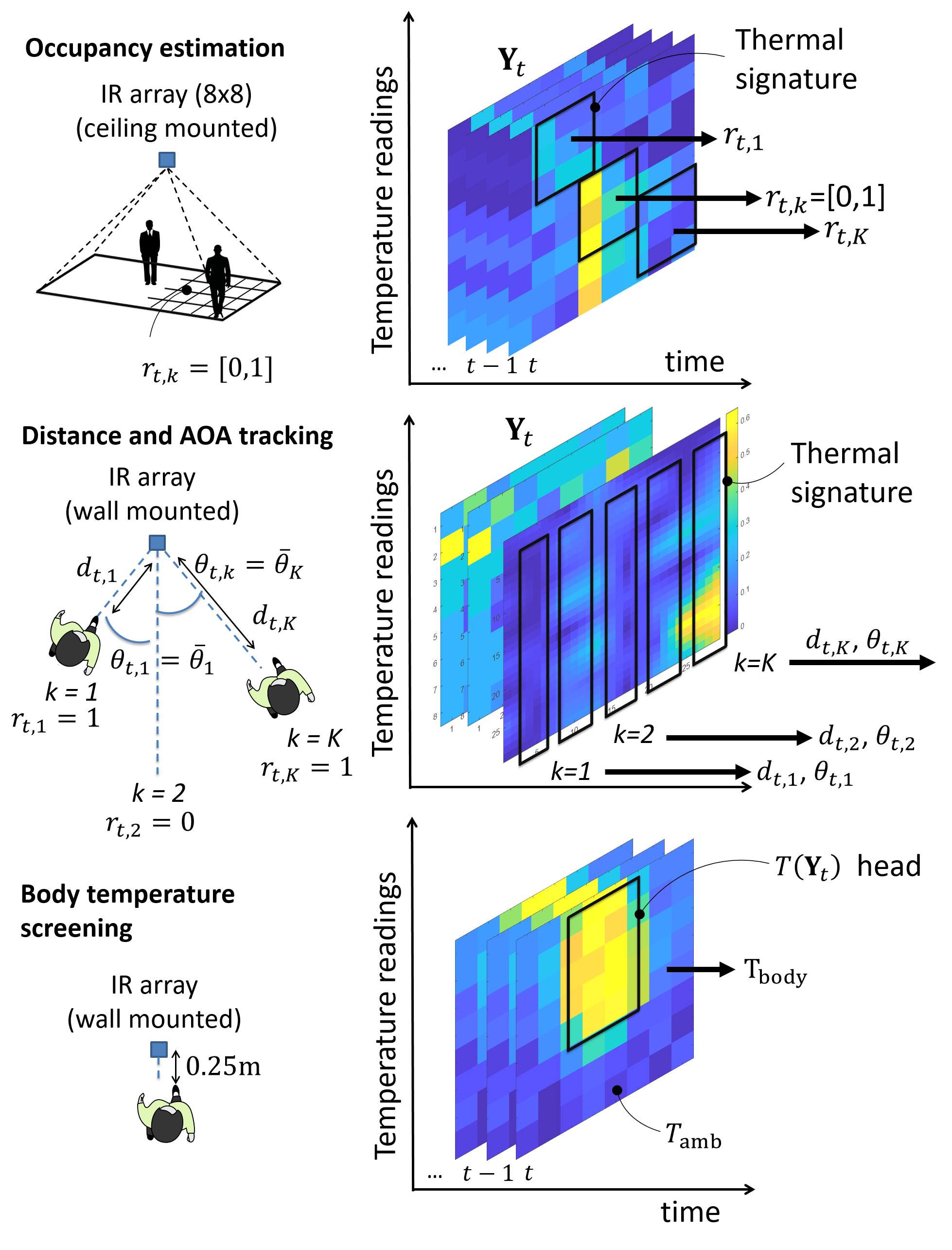
Figure 1: Bayesian models and setups for occupancy estimation, distance/AOA tracking and body temperature screening. Examples of thermal signature backlogs from EnviSense devices [34] are also sketched.

Low-cost passive InfraRed (IR) sensors, also known as thermopiles, are mostly used for subject detection in intrusion alarm systems and lighting applications [5]. Unlike emerging contact tracing applications [6] or other active technologies [7], IR-based sensing systems do not need the cooperation of the monitored subjects. In addition, these systems enable body motion detection, without being limited by privacy issues, since no specific person can be recognized through the analysis of thermal frames and no electronic records are stored. IR sensors also overcome some known computer vision limitations [8], since humans thermal profile does not depend on light conditions. Finally, the analysis of body-induced thermal signatures enable advanced applications, i.e. body occupancy detection, passive localization and tracking [9, 10].

As shown in Fig. 1, the paper targets a system consisting of multiple networked IR sensor arrays detecting the IR radiation in the Long Wavelength InfraRed (LWIR) band. Sensors can be deployed according to different configurations, i.e. wall- or ceiling-mounted. A Bayesian signal processing framework is proposed to optimize both distancing monitoring (localization and counting) and unobtrusive body temperature screening procedures for early diagnosis. The joint analysis of mobility and body temperatures is validated in several indoor operational environments exploiting real field measurements.

I-A Related works

IR sensor arrays [9, 11, 12] have typically low-cost and are characterized by a high temporal and a low spatial resolution. When deployed for monitoring large spaces, multiple arrays can be also placed in selected spots to optimize coverage. Signal processing methods usually apply to raw thermal measurements and target the estimation of human subject(s) space occupancy in real-time, for monitoring body positions, motion intentions such as speed, Direction/Angle Of Arrival (DOA/AOA) [5], and for activity recognition [13]. Existing techniques are mostly based on frame-based computer vision approaches [4]. They consider analytics over individual time-slices (frames) of raw temperature measurements, ranging from K-nearest neighbor (K-NN) classifiers [11, 12], decision trees [14, 15], Kalman filtering [5, 16], support vector machines [8, 13] up to deep convolutional encoder-decoder networks [17]. Typical challenges in thermal vision need to face the temporal disappearance of the subjects [18], due to noisy readings and external heat sources that might be interpreted as false targets. Adaptive background subtraction methods, thresholding or probabilistic methods [19] should be therefore adopted to filter out noisy thermal sources that are not induced by body presence. More recently, the adoption of Bayesian tools over backlogs of thermal images has shown to prevent the problem of human body disappearance [10].

Temperature measurement through contactless devices [20, 21] are becoming attractive as they allow the automatic screening of large populations [22, 23, 24]. Existing automatic systems are capable of providing continuous real-time monitoring at the price of a reduced user’s mobility. However, contactless instruments like thermal camera scanners, have some limitations concerning temperature accuracy, and lack of a standardized processing interface, tools and protocols. Several studies have been conducted to investigate usability and reliability of thermal cameras for fever measurements [19, 25, 26, 27, 28]. Autonomy, size, and costs are generally the main issues limiting the mass diffusion of these devices.

I-B Contributions

The paper focuses on the analysis, design and verification of a unified Bayesian framework for the real-time tracking of body-induced thermal signatures obtained from LWIR sensor arrays arbitrarily deployed in the monitored area. The proposed framework enables three main functions: i) the estimation of the body occupancy in selected spots from which the mutual distance between subjects [29] (i.e., physical distancing) can be inferred; ii) the anonymous tracking of the relative position of the subject(s) with respect to the IR array, namely the distance and the angle of arrival (AOA) of the targets moving in the considered space, and iii) the contactless body temperature screening for subjects located nearby the sensors.

Compared to conventional frame-based methods [8, 9, 11], the proposed framework adopts a statistical model for the extraction of body-induced thermal signatures from noisy data, and a mobility model to track multi-body movements and to avoid false target detection. The approach generalizes the system proposed in [10] to arbitrary sensor deployments, including wall- and ceiling-mounted setups. It can be thus used to assess the combined use of wall- and ceiling-mounted distributed sensors and to improve accuracy or coverage. Body temperature screening [21] is rooted here at Bayesian decision theory: first, a statistical model is proposed to relate the body surface temperature with the noisy IR sensor readings. Next, a method for anomalous body temperature detection is developed to account for variable air/background temperature, noisy heat sources and small voluntary or involuntary body (e.g., head) movements. It also fuses IR data with a radio-frequency (RF) low-cost radar for finer grained head positioning.

The paper is organized as follows: Sect. II introduces the main challenges and assumptions. Focusing on occupancy estimation and distancing, Sect. III targets the problem of body-induced thermal signature modeling, while Sect. IV develops Bayesian filtering methods for real-time subject tracking. Body temperature screening is described in Sect. V, while Sect. VI addresses both best practices and relevant implementation challenges, including sensor calibration, IR and radar data fusion strategies. Finally, the performances of the proposed methods are verified by measurements targeting both industrial and smart living scenarios.

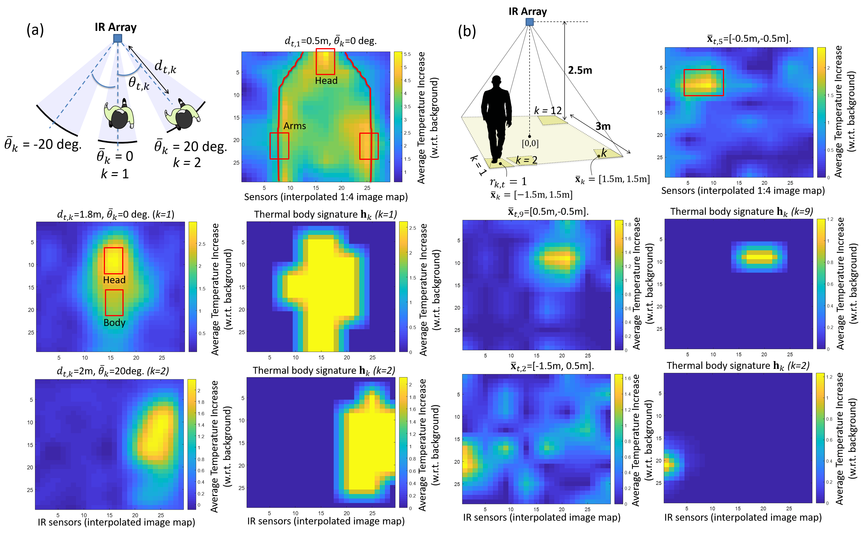
Figure 2: Examples of thermal signatures. (a) Wall-mounted IR sensors: interpolated thermal images (left) and corresponding signatures $\mathbf{h}_{k}=\overline{\sigma}(d_{t,k})\,\mathbf{b}_{k}$ (right) for different body positions (example regions $k=1,2$). (b) Ceiling-mounted IR sensors: thermal images (left) and signatures $\mathbf{h}_{k}=\overline{\sigma}\,\mathbf{b}_{k}$ (right) for different body positions (example regions $k=2,9$).

II System and problem definition

We introduce here the statistical model for the raw thermal data captured by the IR sensor array. This model can serve as a general framework for application to multi-sensor deployments and large IR arrays as well. Sensor readings at time $t$ are collected in the vector $\mathbf{y}_{t}$ of size $M$, $\mathbf{y}_{t}=[y_{t,1},...,y_{t,M}]^{\mathrm{T}}$, assuming $M$ thermopile elements, or detectors (in 1D linear or 2D grid format). In the examples of Fig. 1, the detector array acquires raw thermal IR images organized as 2D frames of $8\times 8$ pixels ($M=64$). For the purpose of localization, the area $\mathcal{X}$ within the Field Of View (FOV) of each IR array sensor is organized into a grid consisting of $K\leq M$ different physical Regions Of Interest (ROI). Each region $k$ (with $1\leq k\leq K$) thus covers a 2D space $\mathcal{X}_{k}$ with $\cup_{k}\mathcal{X}_{k}=\mathcal{X}$. As depicted in Fig. 2(a), for wall-mounted sensors, namely 2D sensor arrays looking inward and deployed in a vertical plane, the $K$ ROIs represent different access areas for the subjects: they are characterized by $\mathbf{\overline{\theta}}_{k}$, namely the target AOA. Subject position is given in terms of distance $d$ and AOA $\theta$ relative to the IR array sensor. Similarly, for ceiling-mounted sensors in Fig. 2(b), namely 2D sensor arrays looking downward and deployed in an horizontal plane, each ROI $k$ is characterized by the relative 2D location footprint $\mathbf{\overline{x}}_{k}$ with respect to the intersection of the vertical axis passing through the sensor array center and the horizontal plane of the floor. Considering both setups (i.e., wall- and ceiling-mounted sensors), the problem we tackle is threefold:

1. to estimate, for all $K$ regions, the occupancy vector $\mathbf{\mathbf{r}}_{t}=[r_{t,1},...,r_{t,k},...,r_{t,K}]^{\mathrm{T}}$ of size $K\times 1$, where $r_{t,k}\in[0,1]$ provides the binary information about the presence of the subject at time $t$ in the $k$-th region;

2. to quantify the relative position of the subject(s) in the estimated region(s), i.e. the relative 2D position of the subject $\Theta_{t,k}=[d_{t,k},\theta_{t,k}]$, with distance $d_{t,k}$ and AOA $\theta_{t,k}$, when crossing the FOV of the corresponding sensor at time $t$;

3. to detect the body temperature of the identified subject $T_{\mathrm{body}}$ via a contactless and non-invasive (i.e., camera-less) approach, triggered by the specific locations occupied by the body.

The occupancy $\mathbf{r}_{t}$ and locations $\Theta_{t,k}$ can be used to count the number of people in the area, to estimate their positions and to monitor the mutual distance between subjects [29] as well. The noisy temperature readings $\mathbf{y}_{t}$ depend linearly on the occupancy pattern $\mathbf{\mathbf{r}}_{t}$ as

$$\mathbf{y}_{t}=\mathbf{H}\cdot\mathbf{\mathbf{r}}_{t}+\mathbf{w}_{t}=\,\sum_{k=1}^{K}\mathbf{h}_{k}\left(\Theta_{t,k}\right)\cdot r_{t,k}+\mathbf{w}_{t},$$ (1)

where each m-th element $y_{t,m}$ of $\mathbf{y}_{t}$ is thus $y_{t,m}=\negthinspace\sum_{k=1}^{K}h_{m,k}(\Theta_{t,k})\cdot r_{t,k}+w_{t,m}$. The matrix $\mathbf{H}=\mathbf{H}(\Theta_{t,k})$,

$$\mathbf{H}(\Theta_{t,k})=[\mathbf{h}_{1},...,\mathbf{h}_{k},....,\mathbf{h}_{K}]$$ (2)

of size $M\times K$ collects the thermal signatures vectors $\mathbf{h}_{k}=\mathbf{h}_{k}\left(\Theta_{t,k}\right)=[h_{1,k}\left(\Theta_{t,k}\right),...,h_{M,k}\left(\Theta_{t,k}\right)]^{\mathrm{T}}$ of size $M\times 1$. Signatures describe the pattern of temperature increases induced by a body occupying the region $k$ at position $\Theta_{t,k}$. Clearly, in absence of the target i.e. for $\Theta_{t,k}=\emptyset$, it is $\mathbf{h}_{k}(\Theta_{t,k})=\mathbf{0}.$ Modeling of $\mathbf{h}_{k}$ in (1) depends on wall or ceiling sensor layouts and it is addressed in the next sections. The background column vector $\mathbf{w}_{t}=[w_{t,1},...,w_{t,M}]^{\mathrm{T}}$ of size $M\times 1$ conveys information about detectors noise and noisy heat-sources that are not caused by body movements but characterize the empty space. This is modeled here as multivariate Gaussian $\mathbf{w}_{t}\sim\mathcal{N}(\boldsymbol{\mu},\mathbf{C})$ described by the average vector $\boldsymbol{\mu}=[\mu_{1},...,\mu_{M}]^{\mathrm{T}}$ and the covariance matrix $\mathbf{C}$.

III Body-induced thermal signature model

Learning of the body-induced thermal signatures in $\mathbf{H}$ and the background/ambient temperature $\left\{\boldsymbol{\mu},\mathbf{C}\right\}$ in (1) can be based on a supervised method, i.e. the conditional maximum likelihood $\widehat{\mathbf{H}}=\mathrm{argmax_{\mathbf{H}}}\mathrm{Pr}\left[\mathbf{y}_{t}\mid\mathbf{\mathbf{r}}_{t};\mathbf{H},\boldsymbol{\mu},\mathbf{C}\right]$ estimator. However, considering the interpolated ($1:4$) thermal image examples of Fig. 2, it is reasonable to assume that the individual elements $h_{m,k}$ of matrix $\mathbf{H}$ are intrinsically sparse [10]. Assuming the linear coefficients of $\mathbf{H}$ to have a Laplace prior distribution [30], and Gaussian background (1), the model $\mathbf{H}$ is estimated using a Least-Squares (LS) method:

$$\widehat{\mathbf{H}}=\mathrm{argmin_{\mathbf{H}}}\sum_{i=1}^{N}\left\|\mathbf{\widetilde{y}}_{t}^{(i)}-\mathbf{H}\cdot\mathbf{\mathbf{r}}_{t}^{(i)}\right\|_{\mathbf{C}}^{2}+\lambda\sum_{m=1}^{M}\sum_{k=1}^{K}\left|h_{m,k}\right|.$$ (3)

This is based on $N$ labeled training measurements collected in the set $\left(\mathbf{\mathbf{r}}_{t}^{(i)},\mathbf{y}_{t}^{(i)}\right)$, namely the thermal frames $\mathbf{\widetilde{y}}_{t}^{(i)}=\mathbf{y}_{t}^{(i)}-\mathbf{\boldsymbol{\mu}}$, $i=1,...,N$, and the corresponding true occupancy patterns $\mathbf{r}_{t}^{(i)}$. A regularization parameter $\lambda=41$ is used for optimization, while $\left\|\mathbf{y}\right\|_{\mathbf{C}}=\mathbf{y}^{T}\mathbf{C}^{-1}\mathbf{y}$ denotes weighting by covariance $\mathbf{C}$. Although the above Lasso-type regularization [30] sets matrix $\mathbf{H}$ to have a sparse representation, the solution is sensitive to training impairments, and thus requires time-consuming calibration. In what follows, we propose a stochastic model for thermal signatures that is less sensitive to such impairments.

TABLE I: Sensor parameters for body localization (thermal signature modeling for physical distancing) and body surface temperature measurement (temperature screening).

Physical distancing	Wall-mounted		$\begin{array}[]{l}\mathbf{h}_{k}(d_{t,k})=\sigma(d_{t,k})\,\mathbf{b}_{k}\textrm{ see eq. (\ref{model_thermal_sign})}\\ \mathbf{b}_{k}:\forall k,\,\tau_{k}=\tau=0.8\,\text{\textdegree}\mathrm{C}\textrm{ (threshold)}\\ \overline{\sigma}(d_{t,k})\textrm{ see eq. (\ref{eq:rect})}\\ d_{min}=0.25\,\textrm{m},\,d_{max}=3.5\,\textrm{m}\\ \sigma_{T}=1.5\,\text{\textdegree}\mathrm{\textrm{C}}\\ \overline{\sigma}_{0}=4.5\,{{}^{\circ}}\mathrm{\textrm{C}},\,\gamma=1.1\mathrm{\,{{}^{\circ}}\textrm{C/m}}\end{array}$
	Ceiling-mounted		$\begin{array}[]{l}\mathbf{h}_{k}=\sigma\,\mathbf{b}_{k}\textrm{ see eq. (\ref{model-1})}\\ \mathbf{b}_{k}:\forall k,\,\tau_{k}=\tau=0.4\,\text{\textdegree}\textrm{C}\textrm{ (threshold)}\\ \overline{\sigma}=1.3\,{}^{\circ}\mathrm{C}\mathrm{\textrm{ (ceiling height $3\,$m)}}\\ \sigma_{T}=0.3\,{}^{\circ}\mathrm{C}\end{array}$
Temperature screening		$\begin{array}[]{l}\alpha_{0}\negthinspace=\negthinspace 0.67,\,\alpha_{1}\negthinspace=\negthinspace 0.45\textrm{ (linear)}\\ \alpha_{0}\negthinspace=\negthinspace 0.66,\,\alpha_{1}\negthinspace=\negthinspace 0.54,\,\alpha_{2}\negthinspace=\negthinspace-\negthinspace 0.21\negthinspace\textrm{ (quad.)\negthinspace}\\ \beta_{0}=1,\,\beta_{1}=-0.09\\ \sigma_{\mathrm{body}}=0.4\,{{}^{\circ}}\textrm{C}\\ \xi=-0.2\\ Q=6\div 12\textrm{ (number of samples)}\end{array}$

III-A Signature modeling for distance and AOA estimation

The proposed simplified model sets the individual thermal signatures $\mathbf{h}_{k}$, namely the columns of $\mathbf{H}$, to depend linearly on the body distances $d_{t,k}$ and have binary and sparse representations. Signatures are thus approximated as

$$\mathbf{h}_{k}(d_{t,k})=\sigma(d_{t,k})\,\mathbf{b}_{k},$$ (4)

where $\sigma(d_{t,k})$ measure the body-induced temperature increase at distance $d_{t,k}$ and

$$\mathbf{b}_{k}=\mathbf{1_{\mathit{y_{t,m}-\mu_{m}>\tau_{\mathit{k}}}}}(y_{t,m}-\mu_{m})$$ (5)

is a binary vector, where $\mathbf{1_{\mathit{x>\tau_{\mathit{k}}}}}(x)$ is the indicator function, namely $\mathbf{1_{\mathit{x>\tau_{\mathit{k}}}}}(x)=1$ if $x>\tau_{\mathit{k}}$ and $\mathbf{1_{\mathit{x>\tau_{\mathit{k}}}}}(x)=0$, otherwise. The threshold $\tau_{\mathit{k}}$ is set, for each region $k$, according to the selected layout. In Tab. I and Sect. VI-A, we assume that $\forall k$ it is $\tau_{\mathit{k}}=\tau$. Coefficient $\sigma(d_{t,k})$ models the temperature increase as a stochastic function of the body distance, $\sigma(d_{t,k})\sim\mathcal{N}(\overline{\sigma}(d_{t,k}),\sigma_{T}^{2})$. The average temperature increase $\overline{\sigma}(d_{t,k})$ follows a smooth rectified linear (s-relu) model

$$\overline{\sigma}(d_{t,k})=\log\left[1+\exp(\overline{\sigma}_{0}-\gamma\cdot d_{t,k})\right],$$ (6)

for $d_{t,k}\geq d_{min}$. Finally, deviation term $\sigma_{T}$ accounts for random, small body movements around the nominal position. Body-induced effects decay almost linearly with the distance from the IR array, with rate $\gamma$: in fact, when the distance increases, not only the body is measured, but also whatever else falls within the spot area, including the background.

Using field measurements collected from $3$ subjects and two environments, as described in Sect. VI, in Fig. 3 we highlight the s-relu model approximation using the parameters shown in Tab. I that are optimized by LS method. Body effects converge smoothly to $\overline{\sigma}(d_{t,k})\simeq 0$ when $d_{t,k}>d_{max}=3.5$ m. Examples of thermal signatures (4) for selected ROIs with AOA $\mathbf{\overline{\theta}}_{k}=\left\{0\text{\textdegree},20\text{\textdegree}\right\}$ are also shown in Fig. 2(a) and compared with the averaged temperature increases $\mathrm{\mathbb{E}}_{t}\left[\mathbf{\widetilde{y}}_{t}^{(i)}\right]$ with respect to the background.

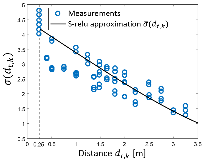
Figure 3: Model $\overline{\sigma}(d_{t,k})$ for wall mounted sensors and its validation from indoor measurements (s-relu approximation).

III-B Signature modeling for occupancy estimation

Considering ceiling-mounted sensors as special case, the distance of the body from the array can be assumed as constant within the sensor FOV. Thus, we further simplify (4) as

$$\mathbf{h}_{k}=\sigma\,\mathbf{b}_{k},$$ (7)

where the term $\sigma$ models the body-induced thermal increase compared to the background. Temperature increases typically fall in the range $\sigma=1.1^{\;\circ}\mathrm{C}\,\div\,1.4{}^{\;\circ}\mathrm{C}$, for $2.5\;\textrm{m}\;\div 3\;\textrm{m}$ ceiling-mounted sensors, and are consistent with the s-relu model (6). Increase $\sigma$ is modelled here by the Gaussian probability density function $\sigma\sim\mathcal{N}(\overline{\sigma},\sigma_{T}^{2})$ where $\overline{\sigma}$ is obtained from (6) using the sensor height from the ground as input distance (here $2.5$ m). For the layout of Sect. VI, Fig. 2(b) shows examples of the signatures $\mathbf{h}_{k}$ for a subject located at selected positions, labelled as $\mathbf{\overline{x}}_{k}$. Signatures are compared with the corresponding averaged temperature increases $\mathrm{\mathbb{E}}_{t}\left[\mathbf{\widetilde{y}}_{t}^{(i)}\right]$.

IV Bayesian filtering for localization

We estimate here, for each region $k$, the body positions $\Theta_{t,k}$, namely the (binary) occupancy $\Theta_{t,k}=\left[r_{t,k}\right]$, or the subject locations $\Theta_{t,k}=\left[d_{t,k},\theta_{t,k}\right],$ by considering an arbitrary sensor layout (wall or ceiling mounts). Following the Bayesian approach, the decision on subject locations is based on the a-posteriori probability $\mathrm{Pr}\left(\Theta_{t,k}\mid\mathbf{Y}_{t}\right)$ conditioned on all the observed temperature measurements $\mathbf{Y}_{t}=[\mathbf{y}_{1},...,\mathbf{y}_{t}]^{T}$ up to time $t$. By defining $\mathrm{Pr}\left(\Theta_{t,k}\mid\mathbf{Y}_{t}\right)=\Lambda_{t,k}$, the probability terms can be evaluated iteratively as [2]

$$\Lambda_{t,k}\propto\Gamma(\mathbf{y}_{t}\mid\Theta_{t,k})\cdot\left(\sum_{h}\mathrm{Pr}(\Theta_{t,k}|\Theta_{t-1,h})\cdot\Lambda_{t-1,h}\right),$$ (8)

being $\Gamma(\mathbf{y}_{t}\mid\Theta_{t,k})=\mathrm{Pr}\left(\mathbf{y}_{t}\mid\Theta_{t,k};\mathbf{h}_{k},\boldsymbol{\mu},\mathbf{C}\right)$ the conditional likelihood and $\mathrm{Pr}\left(\Theta_{t,k}\mid\mathbf{Y}_{t-1}\right)=\sum_{h}\mathrm{Pr}(\Theta_{t,k}|\Theta_{t-1,h})\cdot\Lambda_{t-1,h}$ the a-priori probability. The likelihood function depends on the background temperature ($\boldsymbol{\mu},\mathbf{C}$) and the body-induced thermal signatures $\mathbf{h}_{k}$, defined in (4) or (7) for ceiling- or wall-mounted setups, respectively, as

$$\begin{array}[]{l}\Gamma(\mathbf{y}_{t}\mid\Theta_{t,k})\sim\mathcal{N}\left[\overline{\sigma}\mathbf{b}_{k}+\negthinspace\mathbf{\boldsymbol{\mu}}_{k},\mathbf{C}_{k}+\sigma_{T}^{2}\mathbf{I}\right]\\ \Gamma(\mathbf{y}_{t}\mid\Theta_{t,k}=\emptyset)\sim\mathcal{N}\left[\mathbf{\boldsymbol{\mu}}_{k},\mathbf{C}_{k}\right].\end{array}$$ (9)

The vector $\mathbf{\boldsymbol{\mu}}_{k}=\left\{\mu_{k,q}:\forall q,\text{ $b_{k,q}>0$}\right\}$ considers only the elements from $\mathbf{\boldsymbol{\mu}}$ corresponding to the non-zero indexes of the binary vector $\mathbf{b}_{k}$ (5), while $\mathbf{\mathbf{C}}_{k}=\mathbb{E}_{t}\left[(\mathbf{w}_{t,k}-\boldsymbol{\mu}_{k})(\mathbf{w}_{t,k}-\boldsymbol{\mu}_{k})^{\mathrm{T}}\right]$ is defined similarly using $\mathbf{w}_{t,k}=\left\{w_{t,q}:\forall q,\text{ $b_{k,q}>0$}\right\}$. The transition probability $\mathrm{Pr}(\Theta_{t,k}|\Theta_{t-1,h})$ is computed according to the selected layout-specific mobility model [31].

Algorithm 1 Distancing and AOA tracking

1:procedure tracking($[\mathbf{b}_{k},\overline{\theta}_{k}]_{k=1}^{K},\overline{\sigma}(\cdot),\sigma_{T}^{2},\boldsymbol{\mu},\mathbf{C},[d]_{d=d_{min}}^{d_{max}}$)

2:     initialize multivariate Gaussian functions:

3:     $\mathrm{\mathcal{K}}(\mathbf{C})\leftarrow\left(2\pi\right)^{-\frac{M}{2}}\mathrm{det}(\mathbf{C})^{-\frac{1}{2}}$

4:     $\mathcal{N}\left[\mathbf{y\mathrm{;}}\mathbf{x},\mathbf{C}\right]\leftarrow\mathrm{\mathcal{K}}(\mathbf{C})\exp\left[-\frac{1}{2}(\mathbf{y-x})^{\mathrm{T}}\mathbf{C}^{-1}(\mathbf{y-x})\right]$

5:     $\forall d:\,\mathrm{Pr}(d|h)\leftarrow\mathcal{N}\left[d\mathrm{;}h,\mathrm{W}\right]$$\triangleright$ random walk ($0.5$ m/s)

6:     for each round $t$ do$\triangleright$ Main loop

7:         $\forall k,d$: $\Lambda_{t,k}(d)=\frac{1}{d_{\mathrm{max}}-d_{\mathrm{min}}}$$\triangleright$ initialize $\Lambda_{t,k}(d)$

8:         for $k\leftarrow 1,K$ do$\triangleright$ Occupancy $\widehat{r}_{t,k}$

9:              $\Gamma\left(\mathbf{y}_{t}\mid r_{t,k}=1\right)\leftarrow 0$

10:              $\Gamma\left(\mathbf{y}_{t}\mid r_{t,k}=0\right)\leftarrow\mathcal{N}\left[\mathbf{y}_{t};\mathbf{\boldsymbol{\mu}}_{k},\mathbf{C}_{k}\right]$

11:              for $d\leftarrow d_{min},d_{max}$,$\Delta d$ do

12:                  $\mathbf{x}_{k}\leftarrow\overline{\sigma}(d)\mathbf{b}_{k}+\negthinspace\mathbf{\boldsymbol{\mu}}_{k}$

13:                  $\Gamma\left(\mathbf{y}_{t}\mid d\right)\negthinspace\leftarrow\negthinspace\mathcal{N}\left[\mathbf{y}_{t};\mathbf{x}_{k},\mathbf{C}_{k}+\sigma_{T}^{2}\mathbf{I}\right]$$\triangleright$ (9)

14:                  $\Gamma\negthinspace\left(\negthinspace\mathbf{y}_{t}\negthinspace\mid\negthinspace r_{t,k}\negthinspace=\negthinspace 1\right)\negthinspace\negthinspace\leftarrow\negthinspace\negthinspace\Gamma\negthinspace\left(\negthinspace\mathbf{y}_{t}\negthinspace\mid\negthinspace r_{t,k}\negthinspace=\negthinspace 1\right)\negthinspace+\negthinspace\frac{\Gamma\left(\mathbf{y}_{t}\mid d\right)}{d_{\mathrm{max}}-d_{\mathrm{min}}}$

15:              end for

16:              $\widehat{r}_{t,k}\leftarrow\arg\max_{r_{t,k}\in[0,1]}\Gamma\left(\mathbf{y}_{t}\mid r_{t,k}\right)$

17:         end for

18:         for all $k$ s.t. $\widehat{r}_{t,k}=1$ do$\triangleright$ AOA:$\widehat{\theta}_{t,k}$, dist.: $\widehat{d}_{t,k}$

19:              $\widehat{\theta}_{t,k}\leftarrow\overline{\theta}_{k}$$\triangleright$ AOA

20:              for $d\leftarrow d_{min},d_{max},\Delta d$ do$\triangleright$ a-priori

21:                  if  $\widehat{r}_{t-1,k}=1$ then$\triangleright$ subject at $t-1$

22:                       $\Lambda_{t,k}(d)\negthinspace\negthinspace\leftarrow\negthinspace\negthinspace\sum_{h=d_{min}}^{d_{max}}\negthinspace\mathrm{Pr}(d|h)\times\Lambda_{t-1,k}(h)$

23:                  end if

24:                  $\Lambda_{t,k}(d)\leftarrow$$\Gamma\left(\mathbf{y}_{t}\mid d\right)\Lambda_{t,k}(d)$$\triangleright$ a-posteriori

25:              end for

26:              $\widehat{d}_{t,k}\leftarrow\arg\max_{d}\Lambda_{t,k}(d)$$\triangleright$ distancing

27:         end for

28:     end for

29:end procedure

IV-A Distancing and AOA monitoring

For monitoring body distances and movements $\Theta_{t,k}=\left[d_{t,k},\theta_{t,k}\right]$, we resort to the pseudo-code detailed in the Algorithm 1 and described in the following for wall-mounted IR sensors. As depicted in Fig. 2(a), each ROI $k$ corresponds to a different access area, with AOA $\mathbf{\overline{\theta}}_{k}$ (i.e., azimuth) and unknown distance $d_{t,k}$, but in the range $\left[d_{\mathrm{min}},d_{\mathrm{max}}\right]$. We first detect the access area $\hat{r}_{t,k}$, by solving the occupancy problem. Then, both the AOA $\widehat{\theta}_{t,k}=\overline{\theta}_{k}(\hat{r}_{t,k})$ and the distance estimate $\widehat{\Theta}_{t,k}=\widehat{d}_{t,k}$ (distancing) are considered. Occupancy detection is based on the maximum likelihood (ML) algorithm

$$\widehat{r}_{t,k}=\arg\max_{r_{t,k}\in[0,1]}\mathrm{Pr}\left(\mathbf{y}_{t}\mid r_{t,k}\right)$$ (10)

with $\mathrm{Pr}\left(\mathbf{y}_{t}\mid r_{t,k}=0\right)\sim\mathcal{N}\left[\mathbf{\boldsymbol{\mu}}_{k},\mathbf{C}_{k}\right]$ and

$$\mathrm{Pr}\left(\mathbf{y}_{t}\mid r_{t,k}=1\right)=\int_{d_{\mathrm{min}}}^{d_{\mathrm{max}}}\mathrm{Pr}(d_{t,k}=x)\,\Gamma(\mathbf{y}_{t}\mid\Theta_{t,k})\mathrm{d}x,$$ (11)

where $\Theta_{t,k}$= $\left[d_{t,k},\theta_{t,k}=\overline{\theta}_{k}\right]$ and $d_{\mathrm{min}}\leq d_{t,k}\leq d_{\mathrm{max}}$. The integral function in (11) is implemented as a finite sum with interval $\Delta d=0.25$ m while $\mathrm{Pr}(d_{t,k}=x)$ is assumed to be uniformly distributed as $\mathrm{Pr}(d_{t,k}=x)=\tfrac{1}{d_{\mathrm{max}}-d_{\mathrm{min}}}$.

Distance estimation is computed as

$$\hat{d}_{t,k}=\arg\max_{\widehat{r}_{t,k}=1,\text{ }d_{\mathrm{min}}\leq d_{t,k}\leq d_{\mathrm{max}}}\mathrm{Pr}\left(d_{t,k}\mid\mathbf{Y}_{t}\right)$$ (12)

for all the occupied access areas for which $\widehat{r}_{t,k}=1,$$\forall k$: it is obtained via Bayesian filtering (8) now with $\Lambda_{t,k}=\mathrm{Pr}\left(d_{t,k}\mid\mathbf{Y}_{t}\right)$ and $\Theta_{t,k}$= $\left[d_{t,k}\right]$ where the conditional probability $\mathrm{\mathrm{Pr}(\Theta_{\mathit{t,k}}|\Theta_{\mathit{t\mathrm{-1},h}})}$ is given by a 1D random walk [31]. The subject(s) in the area $k$ may thus move backward or forward along the range segment $\left[d_{\mathrm{min}},d_{\mathrm{max}}\right]$ with AOA $\widehat{\theta}_{t,k}=\overline{\theta}_{k}$.

IV-B Subject counting

Subject counting is drawn from the ceiling-mounted IR sensors. In fact, they can be more easily deployed in crowded areas, compared with wall-mounted setups. Counting requires first to detect the presence $\hat{r}_{t,k}$ of the subjects in the $K$ ROIs, then to identify the number of occupied spots $S_{t}=\sum_{k=1}^{K}\hat{r}_{t,k}$ at time $t$. The goal is to detect critical distancing situations (i.e., crowded areas). We adopt here the Bayesian filtering (8) and track the (binary) occupancy vector $\widehat{\mathbf{r}}_{t}=[\hat{r}_{t,k}]_{k=1}^{K}$ according to the Maximum A Posteriori (MAP) estimate

$$\widehat{\mathbf{r}}_{t}=\arg\max_{r_{t,k}\in[0,1],\forall k=1,...K}\underset{\mathrm{Pr}(\mathbf{r}_{t}\mid\mathbf{Y}_{t})}{\underbrace{\prod_{k=1}^{K}\mathrm{Pr}\left(r_{t,k}\mid\mathbf{Y}_{t}\right)}},$$ (13)

where $\mathrm{Pr}\left(r_{t,k}\mid\mathbf{Y}_{t}\right)\propto\mathrm{Pr}\left(\mathbf{y}_{t}\mid r_{t,k}\right)\mathrm{Pr}\left(r_{t,k}\mid\mathbf{Y}_{t-1}\right)$. Notice that the a-priori probabilities $\mathrm{Pr}\left(r_{t,k}\mid\mathbf{Y}_{t-1}\right)$ are now binary and, as in (8), they can be updated iteratively as

$$\mathrm{Pr}\left(r_{t,k}\mid\mathbf{Y}_{t-1}\right)=\sum\mathrm{Pr}(r_{t,k}\mid\mathbf{r}_{t-1})\mathrm{\;Pr}(\mathbf{r}_{t-1}\mid\mathbf{Y}_{t-1}),$$ (14)

by summing over all (binary) combinations in $\mathbf{r}_{t-1}$. The transition probability $\mathrm{Pr}(r_{t,k}\mid\mathbf{r}_{t-1})$ is drawn from the motion model as shown in the eq. 8 of the reference [10].

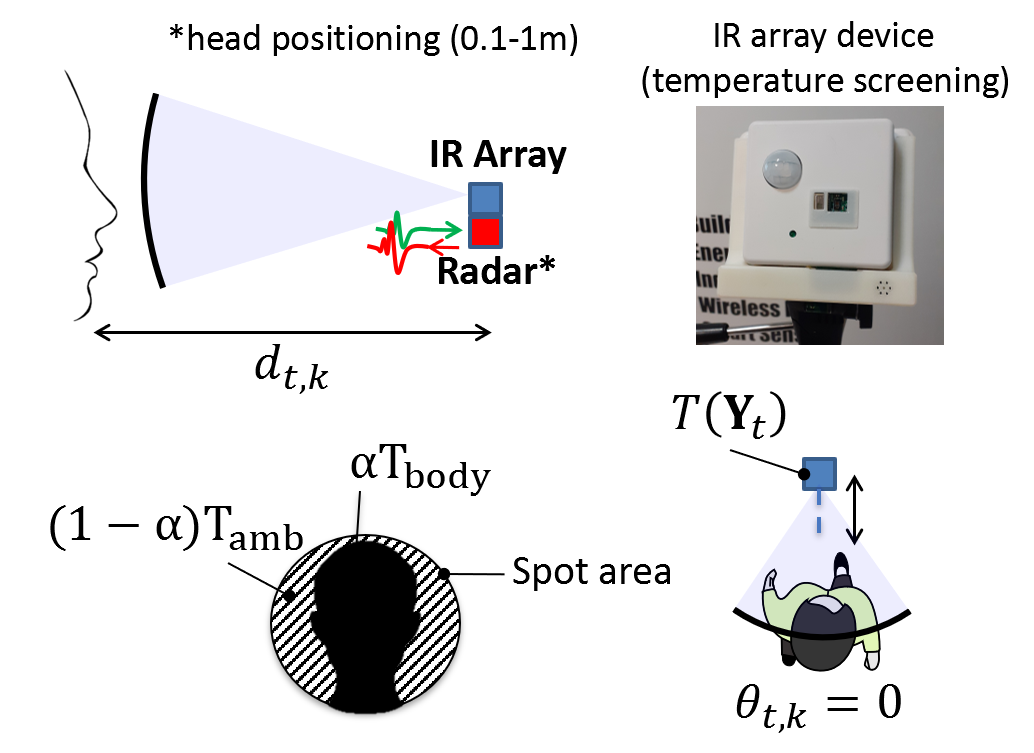
Figure 4: Contactless body screening setup and main parameters.

V Temperature screening

The analysis proposed in this section targets the automation of the temperature screening process, namely the problem of massive and unobtrusive identification of anomalous body temperatures in public environments, where keeping user privacy is critical. The temperature measurement is automatically triggered when the user is located near the IR sensor array. As introduced in Sect. III-A, the temperature readings obtained from the IR sensor do not reveal the precise body temperature, as measurements are influenced by the (time-varying) background and the ambient (i.e., air) temperature $T_{\mathrm{amb}}$. In addition, body-induced effects also decay almost linearly with the distance of the body from the IR sensors.

Compared with state-of-the-art low-cost IR devices [25, 32], the proposed screening method draws from a statistical model and Bayesian decision theory: the user is allowed to move during the screening process while its position is estimated (continuously) using the Bayesian framework proposed in Sect. IV. The screening process gives the probability that the estimated surface body temperature $T_{\mathrm{body}}$ rises above a given threshold $T_{\mathrm{max}}$ ($37.5$ °C). This indicator can be used as initial fever screening, to select the subject(s) that require a more careful treatment (e.g., using manual thermometers or higher-precision devices). Screening precision and recall figures decay with the body distance from the IR array and positioning accuracy: this is quantified in Sect. VI, experimentally.

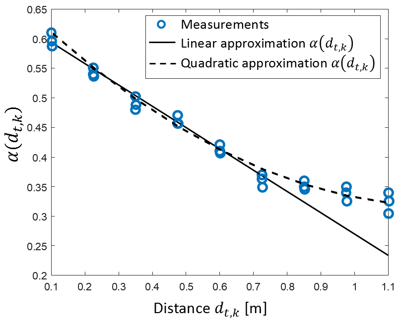
Figure 5: Linear and quadratic models $\alpha(\Theta_{t,k})$ for temperature screening and varying body distance $\Theta_{t,k}=[d_{t,k}]$.

V-A Body surface temperature modeling

Body surface temperature measurement is obtained from sensor readings $\mathbf{y}_{t}$ through the Gaussian function $T(\mathbf{y}_{t})\sim\mathcal{N}(\overline{T}(\mathbf{y}_{t}),\sigma_{\mathrm{body}}^{2})$. The average absolute temperature $\overline{T}(\mathbf{y}_{t})$ is

$$\overline{T}(\mathbf{y}_{t})=\frac{1}{Q}\sum_{\tau\in[t-Q+1,\mbox{ }t]}\max_{m=1,...,M}\left[y_{\tau,m}-\mu_{m}\right]+\mu_{m},$$ (15)

over the inspection interval $[t-Q+1,\mbox{ }t]$ where $\mu_{m}$ is the m-th thermopile background average $\mu_{m}=\mathrm{\mathbb{E}}_{t}\left[y_{t,m}\right]$. The term $\sigma_{\mathrm{body}}^{2}$ accounts for time-varying readings due to random, voluntary or involuntary head/body movements. The (true) body temperature $T_{\mathrm{body}}$ can be obtained as the solution of

$$\beta\overline{T}(\mathbf{y}_{t})=\alpha\,T_{\mathrm{body}}+\left[1-\alpha\right]T_{\mathrm{amb}},$$ (16)

where $T_{\mathrm{amb}}$ corresponds to the ambient temperature. Coefficient $\beta$ models the change of the temperature measurement with $T_{\mathrm{amb}}$, or ambient-to-skin difference [27]. In addition, it corrects the absolute temperature measurement error ($\pm 2.5$ °C typical) observed during initial sensor startup:

$$\beta=\beta_{0}\left(1+\beta_{1}\frac{T_{\mathrm{amb}}-T_{min}}{T_{min}}\right),$$ (17)

with $T_{min}=20{{}^{\circ}}\textrm{C}.$ Ambient temperature $T_{\mathrm{amb}}$ can be obtained directly from the background $\boldsymbol{\mu}$ in (1) as $T_{\mathrm{amb}}=\frac{1}{M}\sum_{m=1}^{M}\mu_{m}$ or drawn from other sensors. Considering a body at distance $d_{t,k}$ and AOA $\theta_{t,k}$, the coefficient $\alpha=\alpha(d_{t,k})$, with $0<\alpha<1$, models the fraction of the sensor spot area size that is occupied by the body (Fig. 4). According to [32], it linearly depends on the body distance $d_{t,k}$ as

$$\alpha(d_{t,k})=\alpha_{0}-\alpha_{1}d_{t,k}.$$ (18)

However, the LS model fitting depicted in Fig. 5 shows that the linear approximation (18) is effective as far as the body distance is lower than $0.75$ m. On the contrary, the quadratic approximation $\alpha(d_{t,k})=\alpha_{0}-\alpha_{1}d_{t,k}-\alpha_{2}d_{t,k}^{2}$, superimposed for comparison on the same figure, gives improvements for larger distances. The experiments in Sect. VI further reveal that the model (15) gives good results as far as $20{{}^{\circ}}\textrm{C}\leq T_{\mathrm{amb}}\leq 28{{}^{\circ}}\textrm{C}.$ Notice that for more general applicability, the relative humidity of the air should be considered as well [24]. All optimized parameters are summarized in Tab. I assuming a FOV of the IR array equal to $60\text{\textdegree}$.

V-B Temperature screening: detection and alerts

Temperature screening discriminates an anomalous body temperature observation ($T_{\mathrm{body}}>T_{\mathrm{max}}$), described here as state $\mathrm{F}_{1}$, from a safe condition ($T_{\mathrm{body}}<T_{\mathrm{max}}$), indicated as $\mathrm{F}_{0}$. Decision at time $t$ is made by collecting $Q$ samples $\mathbf{Y}_{t,Q}=[\mathbf{y}_{t-Q+1},...,\mathbf{y}_{t}]^{T}$ within the inspection interval $[t-Q+1,\mbox{ }t]$. The log-likelihood ratio (LLR) function

$$\mathrm{LLR}(\mathbf{y}_{\mathit{t}})=\mathrm{log}\left[\frac{\Pr\left(\mathbf{y}_{t}|\mathrm{F}_{1}\right)}{\Pr\left(\mathbf{y}_{t}|\mathrm{F}_{0}\right)}\right]$$ (19)

is used as decision metric: for states $\mathrm{F}_{1}$ and $\mathrm{F}_{0}$, the likelihoods are $\mathrm{Pr}\left(\mathbf{y}_{t}|\mathrm{F}_{1};\Theta_{t,k},T_{\mathrm{amb}}\right)$ and $\mathrm{Pr}\left(\mathbf{y}_{t}|\mathrm{F}_{0};\Theta_{t,k},T_{\mathrm{amb}}\right),$ respectively. In particular, using (15) and (16), it is

$$\Pr\left(\mathbf{y}_{t}|\mathrm{F}_{1}\right)\negthinspace=\negthinspace\Pr\left[T(\mathbf{y}_{t})\negthinspace>\negthinspace\alpha T_{\mathrm{max}}\negthinspace+\negthinspace(1\negthinspace-\negthinspace\alpha)T_{\mathrm{amb}}\right]\negthinspace\frac{\Gamma(\mathbf{y}_{t}\mid\Theta_{t,k})}{\mathrm{\Pr\left(\mathrm{F}_{1}\right)}}$$ (20)

being $\Gamma(\mathbf{y}_{t}\mid\Theta_{t,k})=\mathrm{Pr}\left(\mathbf{y}_{t}\mid r_{t,k},\mathbf{h}_{k}\right)$ the conditional likelihood (9) and $\Pr\left[T(\mathbf{y}_{t})\negthinspace>\negthinspace y\right]=\mathcal{Q}\left(\frac{y-\overline{T}(\mathbf{y}_{t})}{\sigma_{\mathrm{body}}}\right)$ with $\mathcal{Q}\left(\cdot\right)$ the Q-function [33]. We also assume that $\mathrm{F}_{0}$ and $\mathrm{F}_{1}$ have the same a-priori probabilities $\Pr\left(\mathrm{F}_{0}\right)=\Pr\left(\mathrm{F}_{1}\right)=1/2$. $\mathrm{Pr}\left(\mathbf{y}_{t}|\mathrm{F}_{0};\Theta_{t,k},T_{\mathrm{amb}}\right)$ is defined similarly and thus omitted.

Being $[t-Q+1,\mbox{ }t]$ the inspection interval, the detector implements a majority voting policy: it votes for state $\mathrm{F}_{1}$ iff

$$\sum_{\tau\in[t-Q+1,\mbox{ }t]}\mathbf{1}_{\mathrm{LLR}(\mathbf{y}_{\tau})\geq\xi}>\sum_{\tau\in[t-Q+1,\mbox{ }t]}\mathbf{1}_{\mathrm{LLR}(\mathbf{y}_{\tau})<\xi}\,.$$ (21)

The detector also outputs a soft indicator, namely the sample probability $\frac{1}{Q}\sum_{\tau\in[t-Q+1,\mbox{ }t]}\mathbf{1}_{\mathrm{LLR}(\mathbf{y}_{\tau})\geq\xi}$, that quantifies the severity of the alert defined in the $\mathrm{[0,1]}$ interval. The optimal threshold value $\xi$ is obtained from a measurement campaign and it is optimized in Sect. VI targeting the maximization of the true positive rates (i.e., or recall figure), as critical for preliminary screening and diagnosis operations.

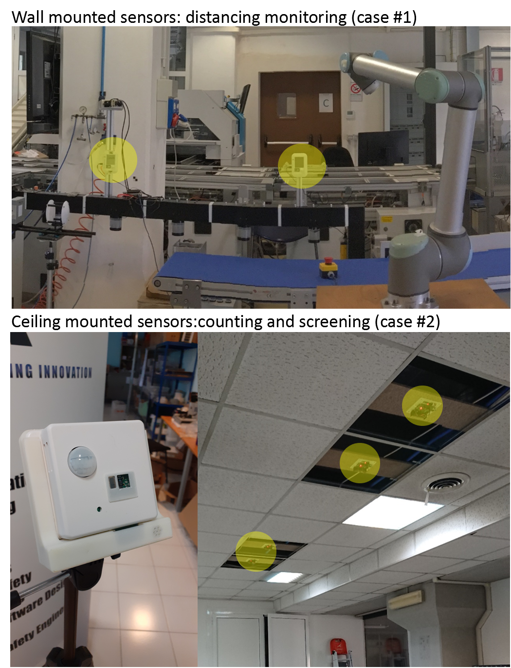
Figure 6: From top to bottom: wall-mounted setup (case #1) and ceiling-mounted (case #2) for different deployments inside the CNR-STIIMA (http://www.stiima.cnr.it/en) test plant.

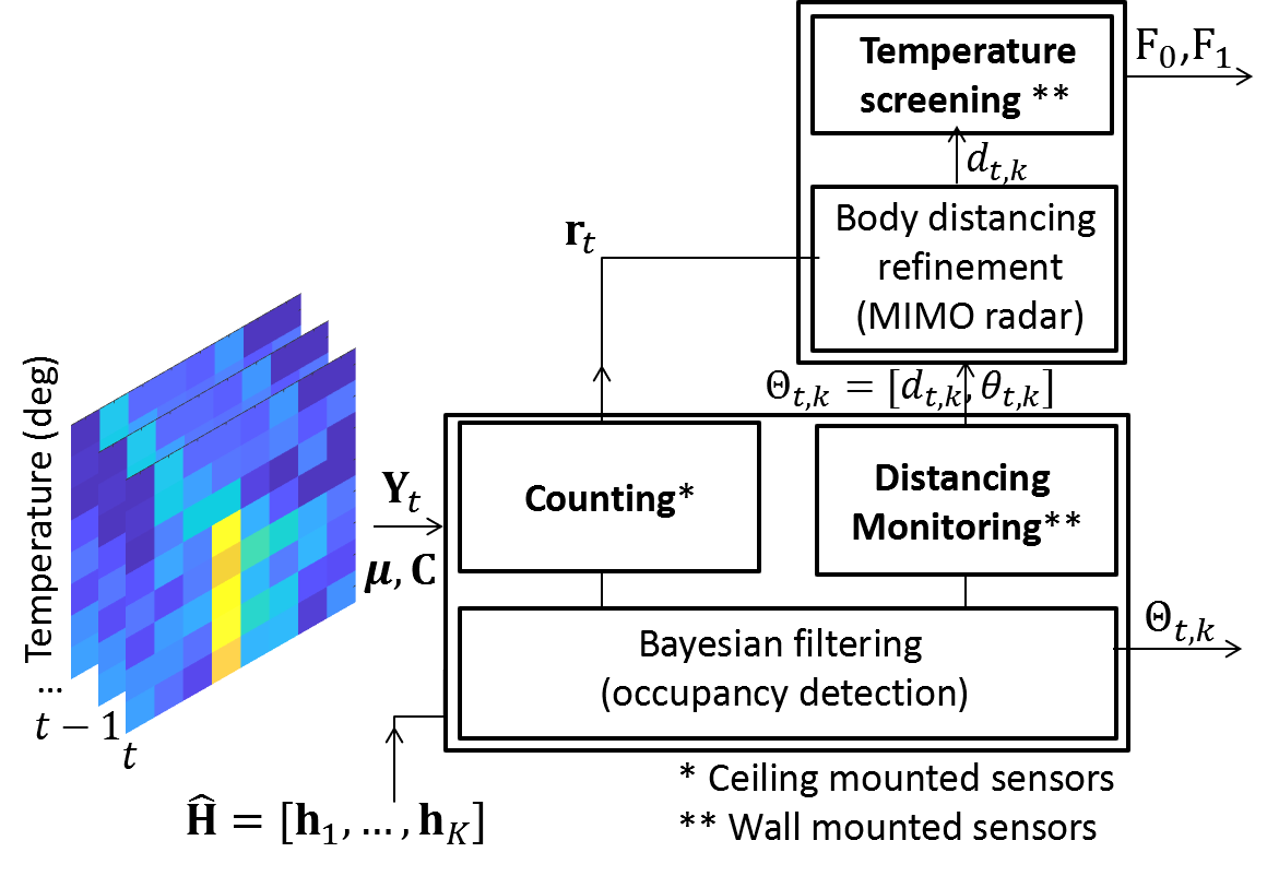
Figure 7: Block diagram for joint occupancy detection, distance monitoring and contactless body temperature screening.

VI Experiments in workspace environments

The experimental validation scenarios exploit IoT devices [34] equipped with thermopile sensor arrays each consisting of $M=64$ IR detectors and FOV of $60\text{\textdegree}$. They are sensible in the $8-13$ $\mu$m LWIR infrared band, with a noise equivalent temperature difference of $\pm 0.08$ °C @ $1$ Hz at room temperature ($T_{\mathrm{amb}}=20$ °C). In the scenario $\#1$ on top of Fig. 6, two wall-mounted devices are installed to monitor the subjects access areas and their distances from a manipulator machine [35], for safety purposes. In the scenario $\#2$ at the bottom of Fig. 6, four devices are mounted on different ceiling panels. They monitor a corridor and count the number of moving subjects, thus analyzing motion patterns in real-time to generate an alert when crowded areas are detected. A wall-mounted device is also installed nearby the entrance for temperature screening while the subject is moving towards the corridor.

The proposed processing framework for joint localization and body temperature screening is summarized in the block diagram of Fig. 7. The IR sensor array readings $\mathbf{Y}_{t}$ are processed continuously and independently for counting, mutual distance monitoring (ceiling-mounted sensors), localization and temperature screening (wall-mounted).

In Sect. VI-A, we first detail the sensor calibration procedures and the necessary initialization stages. Optimized model parameters are summarized in Tab. I. Localization is addressed in Sect. VI-B by analyzing the subject positioning accuracy (distance and AOA) and the ability to identify crowded areas for social distancing monitoring as well.

Finally, temperature screening in Sect. VI-C is corroborated by an experimental study involving both real and simulated body surfaces. The impact of the inspection interval $[t-Q+1,\mbox{ }t]$ and the subject positioning errors on temperature estimation is also discussed. All proposed Bayesian methods (Sect. IV and V) are implemented on a low-power System on Chip (SoC) exploiting a $1.5$ GHz quad core ARM Cortex-A72 processor with 4 GB internal RAM.

TABLE II: Distance and AOA estimation RMSE vs. $\overline{\sigma}_{0}$.

	RMSE		RMSE		RMSE
	$\overline{\sigma}_{0}=4.5{{}^{\circ}}\mathrm{\textrm{C}}$ (Tab. I)		$\overline{\sigma}_{0}=5.5{{}^{\circ}}\mathrm{\textrm{C}}$		$\overline{\sigma}_{0}=3.5{{}^{\circ}}\mathrm{\textrm{C}}$
$d_{t,k}$	$\widehat{\theta}_{t,k}$	$\widehat{d}_{t,k}$	$\widehat{\theta}_{t,k}$	$\widehat{d}_{t,k}$	$\widehat{\theta}_{t,k}$	$\widehat{d}_{t,k}$
$0.5$ m	$8.8^{\circ}$	$0.32$ m	$7.7{{}^{\circ}}$	$0.40$ m	$14.8{{}^{\circ}}$	$0.30$ m
$1.0$ m	$4.9^{\circ}$	$0.28$ m	$4.8{{}^{\circ}}$	$0.45$ m	$10.7{{}^{\circ}}$	$0.28$ m
$1.5$ m	$4.2^{\circ}$	$0.44$ m	$3.7{{}^{\circ}}$	$0.54$ m	$9.2{{}^{\circ}}$	$0.34$ m
$2.0$ m	$4.5^{\circ}$	$0.52$ m	$3.5{{}^{\circ}}$	$0.52$ m	$10.5{{}^{\circ}}$	$0.44$ m
$2.5$ m	$4.2^{\circ}$	$0.67$ m	$3.1{{}^{\circ}}$	$0.70$ m	$10.2{{}^{\circ}}$	$0.51$ m

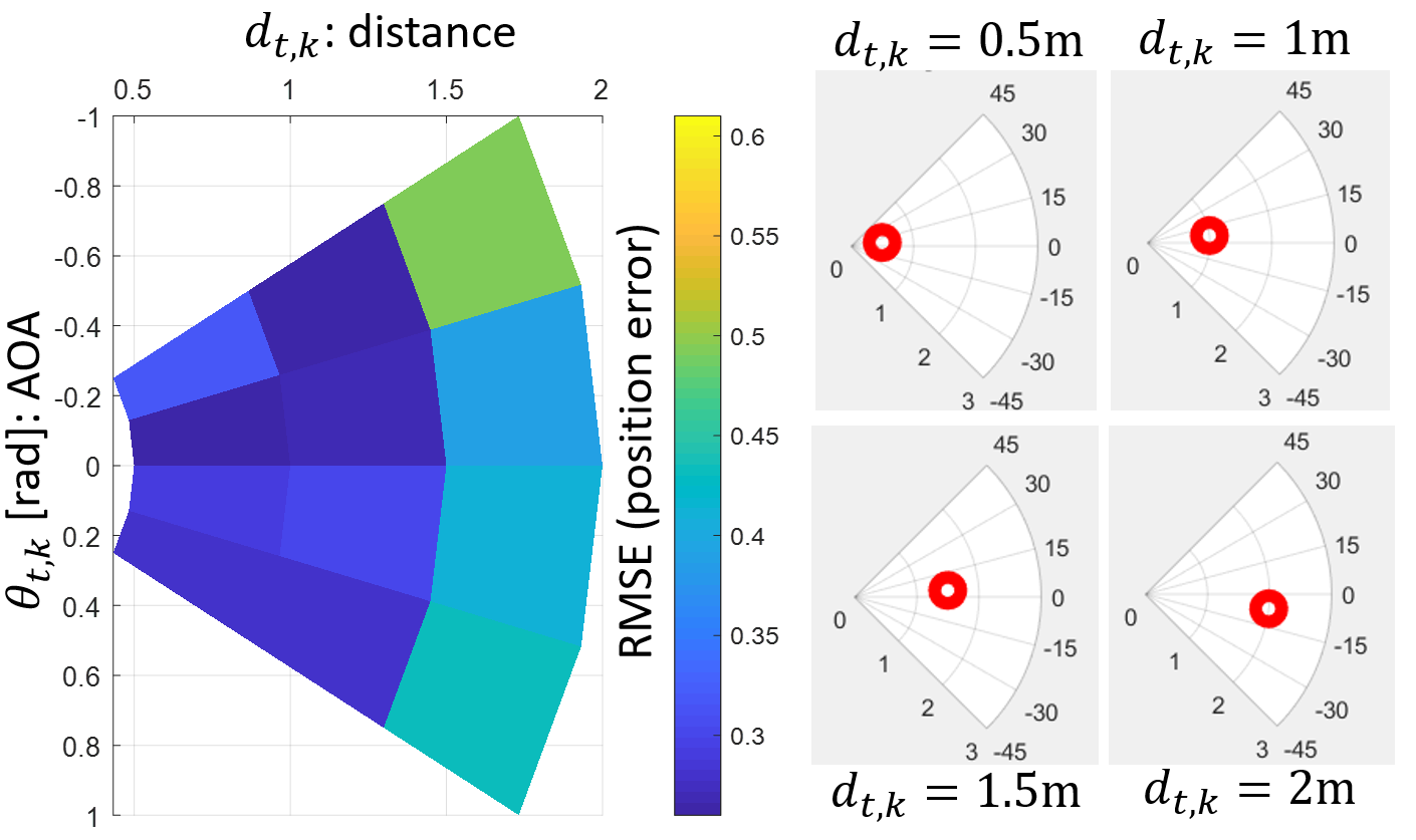
Figure 8: Analysis of localization RMSE for varying subject positions around the IR array and inside the sensor FOV.

VI-A Sensor calibration

Each IoT device samples its IR array every $\triangle t=0.3$ s. Raw data are then forwarded to an intermediate access point via the Thread (IEEE 802.15.4) protocol and sent to a server by exploiting the Message Queuing Telemetry Transport (MQTT) one. The server is in charge of data storage, caching and processing, and acts as a broker accepting subscriptions from an ad-hoc application optimized for visualization of the subject locations in polar or Cartesian coordinates. During initialization, all deployed devices estimate the background parameters $\boldsymbol{\mathbf{\mu}}_{k}$ and $\mathbf{C}_{k}$ in (9) for each location/region $k$. Re-estimation of the parameters $\boldsymbol{\mu}_{k}$ and $\mathbf{C}_{k}$ is required to possibly track time-varying background temperature. It is implemented by a Multivariate Exponentially Weighted Moving Average (MEWMA) and Covariance Matrix (MEWMC) [36], with smoothing constants set to $0.99$ and $0.995$ for the $\boldsymbol{\mathbf{\mu}}_{k}$ and $\mathbf{C}_{k}$ updates, respectively. These are optimized in [10] to track small background changes caused by external thermal sources (e.g., air conditioners, heaters and radiators).

Locations $k$, or access areas, are pre-configured for each sensor (wall- or ceiling-mounted) at installation time. Once the locations $k$ are assigned, the thermal features $\mathbf{h}_{k}$ are computed according to (4) and (7). They consist, for all cases, of the binary functions $\mathbf{b}_{k}$ and the corresponding temperature increases $\sigma\sim\mathcal{N}(\overline{\sigma},\sigma_{T}^{2})$, whose parameters are defined in Tab. I according to the approximation (6). Binary functions depend on the number of areas $K$ to be monitored, and therefore on the sensor layout, so they do not require online training/calibration. Considering ceiling-mounted devices, the observed scene is divided up into $K=12$ ROIs that form a regular grid of $0.5$ m. One individual device can monitor a $2.5$ sqm area when mounted on a $3.0$ m ceiling (faced down). For wall-mounted devices, the monitored area is divided into $K=5$ ROIs representing different access areas for the subjects with corresponding AOAs defined as $\overline{\theta}_{k}=\left\{-30^{\circ},18^{\circ},0^{\circ},18^{\circ},30^{\circ}\right\}$. In all the proposed scenarios, up to $\zeta=3$ bodies might be co-present within the sensor FOV.

Temperature screening adopts the parameters in Tab. I. Notice that the $\beta_{0}$ and $\beta_{1}$ terms depend on the absolute temperature measurement errors and need a re-calibration stage at device start-up. On the contrary, $\alpha_{0},\;\alpha_{1}$ (and $\alpha_{2}$ for the quadratic approximation) do not require re-calibration, as they depend on the geometry of the acquisition (i.e., the physical distance of the subject).

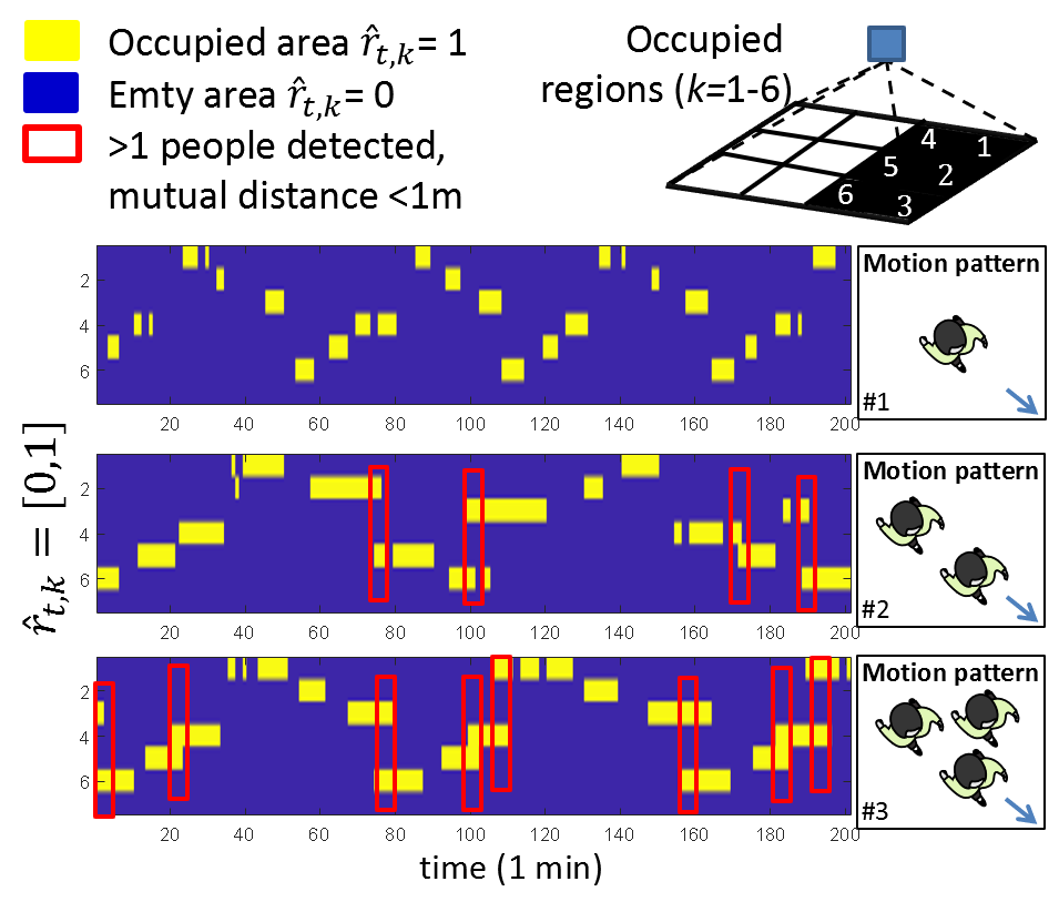
Figure 9: People counting and distancing alerts (red boxes) for ceiling-mounted devices: examples from 3 motion patterns featuring $\zeta=1$ (no alerts) up to $\zeta=3$ subjects.

VI-B Localization and distancing monitoring

In Tab. II, we analyze the performance of distance and AOA estimators, considering a wall-mounted array. Accuracy is given in terms of Root-Mean Squared Error (RMSE). For localization performance verification, we first consider the industrial scenario $\#1$ where we deployed labeled landmarks in selected positions that are occupied by the subject(s) when moving in the area. Estimator errors are thus compared with the true positions from landmarks. The subject is located at (true) distances from the IR array ranging from $d_{t,k}=0.5$ m to $d_{t,k}=2.5$ m and covering access areas with AOAs in the interval $-30^{\circ}\leq\theta_{t,k}\leq 30^{\circ}$.

AOA and distance resolution tradeoff can be controlled by tuning the model parameter $\overline{\sigma}_{0}$: large $\overline{\sigma}_{0}$ values allow to better track subject AOAs, but give incorrect distance estimates, generally larger than the true ones. Smaller $\overline{\sigma}_{0}$ values produce the opposite effect. For subject positioning, we thus choose $\overline{\sigma}_{0}=4.5$ °C, while the other parameters are summarized in Tab. I. The maximum detectable body distance, above which body-induced thermal signatures are almost indistinguishable from the (time-varying) background could be reasonably assumed as $2.5$ m.

In Fig. 8, the RMSE of the location estimate, namely ($\widehat{d}_{t,k},\widehat{\theta}_{t,k}$) is now evaluated as a function of the true target position within the sensor FOV. In all cases, distance estimation error reduces when the subject approaches the sensor, while the situation is reversed for AOA estimation, namely AOA estimation improves when the subject is entering in the sensor FOV. With respect to positioning performance, the IR array thus behaves like a conventional radio-frequency radar as it is sensitive in the range-azimuth domain. Notice that, although not addressed in this paper, subject speed and motion directions could be easily inferred by analyzing the estimated motion pattern over the time domain.

Subject counting and physical/social distancing monitoring are now considered in Fig. 9, using ceiling-mounted devices deployed as shown in the scenario $\#2$ of Fig. 6. In particular, $4$ devices monitor a corridor of $10\times 3$ m: cumulative alerts can be triggered, e.g., every minute/quarter/hour, when the subject mutual distance falls below a threshold (set here to $1$ m), corresponding to two distinct subjects moving in adjacent spots. Alerts give a finer-grained information about space usage and indicate potential criticalities depending on the specific application. Fig. 9 highlights the estimated occupancy patterns $\widehat{\mathbf{r}}_{t}$ (13) versus time considering $6$ selected ROIs, with known 2D location footprint $\mathbf{\overline{x}}_{k=1,...,6}$. Example motion patterns involve $1$ up to $3$ people: subjects moving in adjacent ROIs cause an alert, i.e., a violation of the distancing requirements, highlighted by red boxes. By labeling a (true) violation of distancing limits as true positive, and considering a single IR sensor array, we observe a high precision $99$%, corresponding to negligible false positives, and a recall of $90$%, namely the $90$% of all true violations are correctly identified. Precision is however more critical considering that alerts are typically cumulative, as issued on minute/quarter/hour time-frames. The combined use of multiple IR arrays is also recommended to increase the coverage area.

As previously described, scenarios $\#1$ and $\#2$ cover almost all situations where localization and tracking of people are critical, such as in assisted living, homecare and smart spaces applications. Sensors deployed as in case $\#1$ can be configured to monitor specific locations (e.g., corridors, aisles and access points) by acting as virtual fences not to be trespassed. A single wall-mounted device is sufficient to cover an area with maximum range distance of $2.5$ m and AOAs in the interval $-30^{\circ}\leq\theta_{t,k}\leq 30^{\circ}$. In addition, people intentions (e.g., motion directions and speed) and safety information (e.g., distance from dangerous positions) can be easily inferred. Unlike case $\#1$, in case $\#2$ the devices track people density in small/medium size rooms. In such cases, the ceiling mounted IR arrays should be installed so that the corresponding monitored areas overlap (i.e., $\sim 0.4\div 0,5$ device/sqm density for devices with 3-meter-high rooms). It is worth mentioning that combined wall- and ceiling-mounted devices deployments provide a finer-grained control of the space utilization. These configurations are useful for applications that require the simultaneous distancing monitoring and temperature screening, as detailed in the next Sect. VI-C.

Localization RMSE performance (Table II) is in-line with Bluetooth Low Energy (BLE) based proximity monitoring systems that are based on Received Signal Strength Indicator (RSSI) processing. In smartphone-based contact tracing apps, RSSI values are used to extract relative location estimations, with typical RMSE figures in the range $0.5-1$ m in the short range [6]. Notice that the proposed setup does not need the subject to wear or possess any device; in addition it does not pose any privacy issue as no identity tags are tracked.

With respect to previous works on motion detection through thermal imaging, modified K-NN and decision tree based (C4.5) models reported precision and recall figures in the range of $80\%\div 90\%$ [9, 10, 11, 12] for subject counting ($1\div 4$ people up to a distance of $3$ m). Such figures have been improved (by $5\%\div 7\%$) in [14]. However, these early works did not considered the specific problem of localization and physical distancing monitoring. More recent implementations that use thermal sensor with $M=768$ detectors ($32\times 24$ pixels) achieve an occupancy estimation accuracy of $98\%$ using a modified AdaBoost classifier [17] and considering both ceiling and wall mounted setups.

VI-C Temperature screening: IR and radar sensor fusion

For temperature screening tests, we collected measurements from $3$ different subjects ($2$ male, $1$ female) in healthy condition, namely having $T_{\text{body}}<T_{\text{max}}$. An artificial object with size comparable to the subject (i.e., head) is also adopted to simulate Covid-19 true positives with $T_{\text{body}}>T_{\text{max}}$. During the tests, bodies can freely move around the IR sensor array with distance ranging between $0.1$ m, up to $1.1$ m. Besides the IR sensor array, a low-cost radar [37] working in the mmWave band was co-located (Fig. 6) with the IR sensor array, and used to refine body distance measurements during the screening process. The goal is to obtain a finer-grained estimation of the body location, still preserving the user privacy with respect to camera-based techniques [27, 28]. The radar is equipped with Multiple-Input-Multiple Output (MIMO) antennas ($2$ transmitters, $4$ receivers) and implements a Frequency Modulated Continuous Wave (FMCW) system. It works in the $77-81$ GHz band and allows for precise range (i.e., distance) estimation $\widehat{d}_{t,k}$. The subject positioning algorithm fuses the location estimates produced by the IR sensor array with the ones obtained from the FMCW radar. Data fusion, highlighted in Fig. 7, is built sequentially (boosting method): the location estimate is first obtained by the Bayesian tool presented in Sect. IV (Pseudocode 1), then cross-verified using the radar outputs and corrected, in case of inconsistencies. Combined IR and radar-based positioning gives a localization RMSE of $0.1$ m in the short range ($d_{t,k}\leq 1$ m).

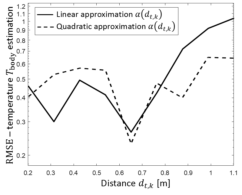
Figure 10: Body temperature estimation RMSE vs. subject distance using the IR sensor array and the mmWave radar ($0.1$ m positioning RMSE at $T_{\text{amb}}=23$ °C). Both linear and quadratic approximations are shown.

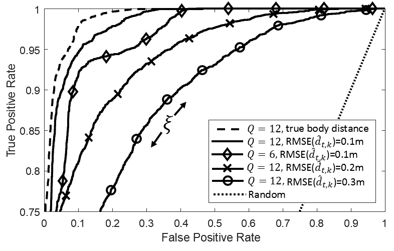
Figure 11: ROC curve for temperature screening (varying number of samples $Q$ and distance estimation accuracies).

Using positioning refinements, temperature estimation is obtained by solving (16). Estimation RMSE is analyzed in Fig. 10 for varying subject distances, and $T_{\mathrm{amb}}=23\text{\textdegree}\mathrm{C}$. Linear and quadratic approximations for $\alpha(d_{t,k})$ in (18) are also compared. The linearized model gives a body temperature estimate with average RMSE of $0.37\text{\textdegree}\mathrm{C}$ for distances lower than $0.75$ m. For larger distances (but still $\leq 1.1$ m), the quadratic approximation performs better, although the RMSE increases up to $0.45\,\text{\textdegree}\mathrm{C}$. The maximum body distance for screening could be thus reasonably set to $1$ m.

In Fig. 11, we analyze the Receiver Operating Characteristic (ROC) figures for varying number of samples ($Q=6,12$) and positioning accuracy, with body location RMSE ranging from $0.10$ m to $0.32$ m. The ROC curve using true body distance information is also superimposed in dashed line as benchmark while the random (i.e., trivial) detector is shown as well. In particular, we consider $2888$ true negative examples, namely healthy subjects with $T_{\mathrm{body}}$ ranging from $36$ °C to $37.2$ °C, and $1800$ true positives, with $T_{\mathrm{body}}$ ranging from $37.8$ °C to $38.5$ °C. True temperatures are measured by a contact thermometer. Pre-screening inspection systems [28] need high true positive rates (TPR), or recall, to maximize the number of subjects correctly detected as unhealthy. In addition, false positive rates (FPR) should be kept as low as possible to limit post-screening operations. Considering $Q=12$ samples, corresponding to an inspection interval of $\sim 4$ seconds, the TPR and the FPR are $97\%$ and $15\%$, respectively, for the detector threshold set to $\xi=-0.2$ (optimized for maximum recall), and subject positioning RMSE of $0.1$ m. Distancing errors have larger impact on screening performance, compared to inspection interval $Q$. In fact, reducing the inspection interval to $\sim 2$ seconds ($Q=6$) brings down the TPR to $94$% and increases the FPR to $18\%$. Positioning errors (RMSE $0.2$ m) are still acceptable but reduce the TPR to $92\%$ and and increase the FPR to $25\%$. Screening performance experiences further degradation for larger RMSE.

TABLE III: Temperature screening for $Q=12$ and $\xi=-0.2$: precision and recall figures using IR sensor and data fusion with radar for distancing refinement.

	IR sensor only		Radar + IR sensor
	(RMSE $0.32$ m)		(RMSE $0.10$ m)
	Recall	Precision	Recall	Precision
$\mathrm{F}_{1}:T_{\mathrm{body}}>T_{\mathrm{max}}$	$88.0\%$	$79.1\%$	$97.0\%$	$87.5\%$
$\mathrm{F}_{0}:T_{\mathrm{body}}<T_{\mathrm{max}}$	$84.0\%$	$88.1\%$	$90.4\%$	$98.0\%$

Considering the same examples, precision and recall figures are now compared in Tab. III using both radar and IR array for distance monitoring. The wall-mounted IR-based devices configured for localization gives an RMSE of $0.32$ m (as in Tab. II) while screening precision and recall are $79.1\%$ and $88\%$, respectively. The combined use of the IR array and the radar gives an RMSE of $0.1$ m and thus improve both figures that are now $87.5\%$ and $97\%$, respectively. These results are in-line with RGB-thermal image-based screening tools with SVM classification [28] that report a recall figure equal to $85.7\%$ and a specificity, namely $1-\mathrm{FPR},$ equal to the $90.1\%$ one. In the same reference [28], conventional fever screening methods based on electronic thermometers show recall and specificity values equal to $60.7\%$ and $86.4\%$, respectively.

VII Conclusions

The paper proposed a Bayesian tool for joint body localization and temperature screening that is based on the real-time analysis of infrared (IR) body emissions using devices equipped with low-cost thermopile-type passive IR sensor arrays. A statistical model is validated experimentally in an industrial test plant to represent the thermal signatures induced by bodies at different locations. The model is general enough to support different device layouts (ceiling- and wall-mounted devices) and it has been verified experimentally targeting the passive detection of body motion directions, distances from the sensor and mutual body distances, to monitor crowded areas. Thus, the proposed sensing platform can be easily adapted for applications ranging from assisted living to homecare, and smart spaces. Contactless temperature pre-screening, rooted at Bayesian decision theory, is integrated with body localization that fuses IR emissions and backscattered radar signals for finer-grained positioning. It thus allows non-invasive body diagnosis by letting the subject freely move in the surroundings of the IR sensor, during the measurement process. Screening is designed to minimize false negatives with performances that are in-line with state of the art inspection tools, but, preserving subject privacy by avoiding imaging from video cameras.

Appendix: Envisense system description

The infra-red array sensor is supported by the multi-sensor box Envisense Smart equipped with a 2.4 GHz IEEE 802.15.4 radio interface. The infra-red array performs $10$ measurements per second of the thermal profile of the space in front of itself, with a range of coverage that reaches up to $7$ m and an angular opening of $60$ deg. Sensors are identified by a unique 64-bit number corresponding to the address of their IEEE 802.15.4 radio module. They transmit infra-red array data with a low-power 2.4 GHz mesh network, each 8x8 thermal map sampled at 10 Hz is sent to the data collector called EnviCore. The thermal map sample is quantized with 8-bits representing the temperature ranging from 0 to 64 °C with a 0.25 °C resolution. Data collected by the gateway is converted to a JSON data packet, marked with a absolute timestamp in order to keep the timing information and allow the synchronization with other sensors data. Finally, all collected and converted data is sent to the processing server by a Wi-Fi connection and MQTT protocol. In order to have the platform working the following configurations steps shall be done: i) EnviSense configuration using the Android App and a smartphone with NFC support; ii) EnviCore configuration with its web pages; iii) processing server configuration.

In order to configure the Envisense device an Android App is provided. The Android Smartphone used for configuration must have NFC technology support in order to communicate with the EnviSense. After the app is launched the configuration is read by simply moving close the smartphone to the device between the solar panel and the PIR. As soon as the configuration is read all sensors are enabled. See [34] for further technical information.

References

- [1] M. Youssef, et al., “Transformative Computing and Communication,” Computer, vol. 52, no. 7, pp. 12-14, July 2019.
- [2] S. Savazzi, et al., “Device-Free Radio Vision for assisted living: Leveraging wireless channel quality information for human sensing,” IEEE Signal Processing Magazine, vol. 33, no. 2, pp. 45-58, Mar. 2016.
- [3] A. Haque, et al., “Illuminating the dark spaces of healthcare with ambient intelligence”, Nature 585, pp. 193–202,2020.
- [4] R. Gade, et al., “Thermal cameras and applications: a survey,” Machine Vision and Applications, vol. 25, no. 1, pp. 245–262, Jan. 2014.
- [5] P. Zappi, et al., “Tracking motion direction and distance with pyroelectric IR sensors,” IEEE Sensors Journal, vol. 10, no. 9, pp. 1486–1494, Sept. 2010.
- [6] N. Ahmed et al., “A Survey of COVID-19 Contact Tracing Apps,” IEEE Access, vol. 8, pp. 134577-134601, 2020.
- [7] M. Marschollek, et al., “Wearable sensors in healthcare and sensor-enhanced health information systems: all our tomorrows?,” Healthcare informatics research, vol. 18, no. 2, pp. 97-104, 2012.
- [8] Z. Chen, et al., “Infrared ultrasonic sensor fusion for support vector machine based fall detection,” Journal of Intelligent Material Systems and Structures, vol. 29, no. 9, pp. 2027–2039, 2018.
- [9] A. Tyndall, et al., “Occupancy estimation using a low-pixel count thermal imager,” IEEE Sensors Journal, vol. 16, no. 10, pp. 3784–3791, May 2016.
- [10] S. Savazzi, et al., “Occupancy Pattern Recognition with Infrared Array Sensors: A Bayesian Approach to Multi-body Tracking,” Proc. of the IEEE International Conference on Acoustics, Speech and Signal Processing (ICASSP’19), Brighton, UK, pp. 4479-4483, 2019.
- [11] J. Tanaka, et al., “Low power wireless human detector utilizing thermopile infrared array sensor,” Proc. of IEEE Sensors, pp. 461-465, Valencia, Spain, Nov. 2014.
- [12] A. Beltran, et al., “Thermosense: Occupancy thermal based sensing for hvac control,” Proc. of the 5th ACM Workshop on Embedded Systems For Energy-Efficient Buildings (BuildSys’13), pp. 1-8, Nov. 2013.
- [13] S. Mashiyama, et al., “Activity recognition using low resolution infrared array sensor,” Proc of IEEE International Conference on Communications (ICC), pp. 495–500, Jun. 2015.
- [14] L. Walmsley-Eyre, et al., “Hierarchical classification of low resolution thermal images for occupancy estimation,” Proc. of IEEE 42nd Conference on Local Computer Networks Workshops (LCN Workshops), pp. 9–17, Oct. 2017.
- [15] P. Hevesi, et al., “Monitoring household activities and user location with a cheap, unobtrusive thermal sensor array,” Proceedings of the 2014 ACM International Joint Conference on Pervasive and Ubiquitous Computing (UbiComp ’14), New York, NY, USA, pp. 141–145, 2014.
- [16] S. Jin Lee, et al., “Human tracking with an infrared camera using a curve matching framework,” EURASIP Journal on Advances in Signal Processing, vol. 2012, no. 1, pp. 99, May 2012.
- [17] A. Naser, et al., “Adaptive Thermal Sensor Array Placement for Human Segmentation and Occupancy Estimation,” IEEE Sensors Journal, 2020..
- [18] Y. Jeong, et al., “Probabilistic method to determine human subjects for low-resolution thermal imaging sensor,” Proc. of IEEE Sensors Applications Symposium (SAS), Feb 2014, pp. 97–102.
- [19] J. Güttler, et al., “Contactless fever measurement based on thermal imagery analysis,” Proc. of IEEE Sensors Applications Symposium (SAS), Catania, 2016, pp. 1-6, 2016.
- [20] A. Dittmar, et al., “A Non Invasive Wearable Sensor for the Measurement of Brain Temperature,” International Conference of the IEEE Engineering in Medicine and Biology Society, New York, pp. 900-902, 2006.
- [21] H.-Y. Chen, et al., “Investigation of the Impact of Infrared Sensors on Core Body Temperature Monitoring by Comparing Measurement Sites,” Sensors, vol. 20, no. 10, art. 2885, 2020.
- [22] S. Amendola, et al., “Design, Calibration and Experimentation of an Epidermal RFID Sensor for Remote Temperature Monitoring,” IEEE Sensors Journal, vol. 16, no. 19, pp. 7250-7257, Oct., 2016.
- [23] E.J.S. Chaglla, et al., “Measurement of Core Body Temperature Using Graphene-Inked Infrared Thermopile Sensor,” Sensors, vol. 18, no. 10, art. 3315, 2018.
- [24] A. Psikuta, et al., “Effect of ambient temperature and attachment method on surface temperature measurements,” International journal of biometeorology, vol. 58, 2013..
- [25] A.V. Nguyen, et al., “Comparison of 3 infrared thermal detection systems and self-report for mass fever screening,” Emerging infectious diseases, vol. 16, no. 11, pp. 1710-1717, Nov. 2010.
- [26] C.C. Liu, et al., “Limitations of forehead infrared body temperature detection for fever screening for severe acute respiratory syndrome,” Infection Control, vol. 25, no. 12, pp. 1109-1111, 2004.
- [27] L.S. Chan, et al., “Screening for fever by remote sensing infrared thermographic camera,” Journal of travel medicine, vol. 11, no. 5, pp. 273-279, 2004.
- [28] T. Negishi, et al., “Contactless vital signs measurement system using RGB-thermal image sensors and its clinical screening test on patients with seasonal influenza,” Sensors (Basel), vol. 20, no. 8, art. 2171, Apr. 13, 2020.
- [29] M. Cristani, et al., “The Visual Social Distancing Problem,” IEEE Access, vol. 8, pp. 126876-126886, 2020.
- [30] R. Tibshirani, “Regression shrinkage and selection via the Lasso: A retrospective,” J. R. Statist. Soc. B, vol. 73, pp. 273-282, 2011.
- [31] G. F. Lawler, et al., “Random walk: a modern introduction,” vol. 123. Cambridge University Press, Jun. 2010.
- [32] A. Manoi, et al., “Size-of-source Effect in Infrared Thermometers with Direct Reading of Temperature,” International Journal of Thermophysics, vol. 38, art. 101, 2017.
- [33] I.M. Tanash, et al., “Global Minimax Approximations and Bounds for the Gaussian Q-Function by Sums of Exponentials,” IEEE Transactions on Communications, vol. 68, no. 10, pp. 6514-6524, Oct. 2020.
- [34] Cognimade S.r.l., Envisense datasheet, Available online: http://www.cognimade.com/project/envisense-industrial/, accessed 10/28/2020.
- [35] S. Kianoush, et al., “Device-Free RF Human Body Fall Detection and Localization in Industrial Workplaces,” IEEE Internet of Things Journal, vol. 4, no. 2, pp. 351-362, Apr. 2017.
- [36] D.M. Hawkins, et al., “Multivariate exponentially weighted moving covariance matrix,” Technometrics, vol. 50, no. 2, pp. 155–166, 2008.
- [37] S. Kianoush, et al., “A Multisensory Edge-Cloud Platform for Opportunistic Radio Sensing in Cobot Environments,” IEEE Internet of Things Journal, 2020.