First-Kind Boundary Integral Equations for the Dirac Operator in 3D Lipschitz domains

Abstract

We develop novel first-kind boundary integral equations for Euclidean Dirac operators in 3D Lipschitz domains. They comprise square-integrable potentials and involve only weakly singular kernels. Generalized Gårding inequalities are derived and we establish that the obtained boundary integral operators are Fredholm of index zero. Their finite dimensional nullspaces are characterized and we show that their dimensions are equal to the number of topological invariants of the domain’s boundary, in other words, to the sum of its Betti numbers. This is explained by the fundamental discovery that the associated bilinear forms agree with those induced by the 2D Dirac operators for surface de Rham Hilbert complexes whose underlying inner-products are the non-local inner products defined through the classical single-layer boundary integral operators for the Laplacian. Decay conditions for well-posedness in natural energy spaces of the Dirac system in unbounded exterior domains are also presented.

31A10, 45A05, 45E05, 45P05, 35F15, 34L40, 35Q61

1 Introduction

We develop first-kind boundary integral equations for the Hodge-Dirac operator in 3-dimensional Euclidean space

(1) $$\mathsf{D}\mathrel{\mathop{\ordinarycolon}}=\mathbf{d}+\bm{\delta}\mathrel{\mathop{\ordinarycolon}}\mathbf{H}(\mathbf{d},\Omega^{\mp})\cap\mathbf{H}(\bm{\delta},\Omega^{\mp})\rightarrow L^{2}(\Omega^{\mp})^{8},$$

involving the exterior derivative and codifferential

(2) $$\mathbf{d} \mathrel{\mathop{\ordinarycolon}}=\begin{pmatrix}0&\mathbf{0}^{\top}&\mathbf{0}^{\top}&0\\ \hbox{\pagecolor{black!10!white}$\displaystyle\nabla$}&\mathbf{0}_{3\times 3}&\mathbf{0}_{3\times 3}&\mathbf{0}\\ \mathbf{0}&\hbox{\pagecolor{black!10!white}$\displaystyle\mathbf{curl}$}&\mathbf{0}_{3\times 3}&\mathbf{0}\\ 0&\mathbf{0}^{\top}&\hbox{\pagecolor{black!10!white}$\displaystyle\text{div}$}&0\end{pmatrix} \bm{\delta} \mathrel{\mathop{\ordinarycolon}}=\begin{pmatrix}0&\hbox{\pagecolor{black!10!white}$\displaystyle-\,\text{div}$}&\mathbf{0}^{\top}&0\\ \mathbf{0}&\mathbf{0}_{3\times 3}&\hbox{\pagecolor{black!10!white}$\displaystyle\mathbf{curl}$}&\mathbf{0}\\ \mathbf{0}&\mathbf{0}_{3\times 3}&\mathbf{0}_{3\times 3}&\hbox{\pagecolor{black!10!white}$\displaystyle-\nabla$}\\ 0&\mathbf{0}^{\top}&\mathbf{0}^{\top}&0\end{pmatrix}.$$ and

We are concerned with the partial differential equations $\mathsf{D}\vec{\mathbf{U}}=\vec{\mathbf{F}}$, which in components $\vec{\mathbf{U}}=\left(U_{0},\mathbf{U}_{1},\mathbf{U}_{2},U_{3}\right)^{\top}$ and $\vec{\mathbf{F}}=\left(F_{0},\mathbf{F}_{1},\mathbf{F}_{2},F_{3}\right)^{\top}$ read

(3) $$-\,\text{div}\,\mathbf{U}_{1} =F_{0},$$

$$\nabla\,U_{0}+\mathbf{curl}\,\mathbf{U}_{2} =\mathbf{F}_{1},$$

$$-\,\nabla U_{3}+\mathbf{curl}\,\mathbf{U}_{1} =\mathbf{F}_{2},$$

$$\text{div}\,\mathbf{U}_{2} =F_{3}.$$

We will consider both interior and exterior boundary value problems, and assume that (3) is either posed on a bounded domain $\Omega^{-}$ having a Lipschitz boundary $\Gamma\mathrel{\mathop{\ordinarycolon}}=\partial\Omega^{-}$, or on the unbounded complement $\Omega^{+}\mathrel{\mathop{\ordinarycolon}}=\mathbb{R}^{3}\backslash\overline{\Omega^{-}}$. In the latter case, suitable decay conditions at infinity will be needed. Throughout, $\Omega\in\{\Omega^{-},\Omega^{+}\}$.

1.1 Related work

Current work discussing Dirac operators from the point of view of Hodge theory offers solutions to boundary value problems for (3) and related eigenvalue problems based on domain variational formulations [26, 13].

The operator matrix in (1) appears under a change of variables in the works of M. Taskinen, S. Vänskä and P. Ylä-Oijala [43, 41, 42] as R. Picard’s extended Maxwell operator. It was originally assembled by R. Picard by combining the first-order Maxwell operator with the principal part of the equations of linear acoustics [34, 35, 25]. In [43, 41, 42], Helmholtz-like boundary value problems for Picard’s operator are studied with a focus on second-kind boundary integral equations.

Eigenvalue problems related to acoustic and electromagnetic scattering, that is transmission problems for the so-called perturbed Dirac operator, have also guided the study of second-kind boundary integral equations in the literature of harmonic and hypercomplex analysis. Important contributions were made in that direction by E. Marmolejo-Olea, I. Mitrea, M. Mitrea, Q. Shi [28], A. Axelsson, A. Rosén and J. Helsing [4, 20, 36]. There, the Dirac operator enters larger systems of equations that encompass or correspond to Maxwell’s equations [28, 20]. An extensive body of work, created by these authors together with R. Grognard and J. Hogan [5], S. Keith [6], A. McIntosh and S. Monniaux [30, 31], is devoted to the harmonic analysis of Dirac operators in $L_{p}$ spaces [7, 29].

1.2 Our contributions

In this work, we derive novel first-kind boundary integral equations for the Dirac equation $\mathsf{D}\vec{\mathbf{U}}=0$ with suitable boundary and decay conditions. Two boundary integral operators are obtained and shown to satisfy generalized Gårding inequalities, making them Fredholm of index $0$. Their finite dimensional nullspaces are characterized in Section 7, where we show that their dimension equals the number of topological invariants of the boundary—counted as the sum of its Betti numbers. Indeed, the integral representations of their associated bilinear forms turn out to be related to the variational formulations of the surface Dirac operators introduced in Section 8. Recognizing these surface operators will simultaneously reveal how the boundary integral operators introduced in Section 5, which are related to two different sets of boundary conditions, arise as “rotated” versions of one another. The exterior representation formula of Lemma 4.24 and the condition at infinity identified in (95) eventually lead, together with the coercivity results of Section 6, to well-posedness of Euclidean Dirac exterior boundary value problems in natural energy spaces in the complement of the finite dimensional nullspaces.

The new integral formulas display desirable properties: the surface potentials are square-integrable and the kernels of the bilinear forms associated with the boundary integral operators are merely weakly singular, i.e. they are bounded by $\mathinner{\!\left\lvert x-y\right\rvert}^{-\alpha}$, $\alpha<2$, cf. [24, Sec. 2.4]. Nevertheless, we want to emphasize that the main result is the discovery that they relate to the Hodge–Dirac operators of surface de Rham Hilbert complexes equipped with the non-local inner products defined as the bilinear forms associated with the classical single-layer potential for the Laplacian. As a consequence, we already know a lot about these first-kind boundary integral operators for the Dirac operator. Moreover, this relationship suggests that they are related to the first-kind boundary integral operators for the Hodge–Laplacian.

For the sake of readability, we adopt the framework of classical vector analysis rather than exterior calculus. It is in this framework that the structural relationship between the following development and the standard theory for second-order elliptic operators seemed most explicit.

In summary, our main contributions are:

• We derive representation formulas for the Dirac equation posed on domains having a Lipschitz boundary by following the approach pioneered by M. Costabel [16]. The novelty here is to follow and extend the elegant strategy used in [14]—there used to find a representation formula for Hodge–Laplace and Helmholtz operators—that leads to potentials having simple explicit expressions. By adapting the arguments in the now classical monographs by W. McLean [32, Chap. 7] and A. Sauter and C. Schwab [37, Chap. 3], we also establish an exterior representation formula. We will observe that the development of this theory is possible due to the strong structural similarity between integration by parts for the first-order Dirac operator and Green’s second formula for second-order elliptic operators.

• A sneak peek at the potentials presented in (68) and (71) will already convince the reader that the approach we have adopted leads to simple formulas for the square-integrable potentials involved in the representation formula. Some terms are recognizable from [14, 15], while others occur in well-known theory for elliptic second-order operators. The simplicity that comes with the calculation procedure provided by Lemma 4.8 allows for a straightforward analysis of their mapping and jump properties.

• Given the previous items, it is not surprising that decay conditions at infinity for exterior boundary value problems posed on the unbounded domain $\Omega^{+}$ can be easily established by adapting the approach for second-order elliptic operators presented in [32, Chap. 7].

• The crux of our calculations are the formulas (110) and (111) for the bilinear forms associated with the obtained weakly-singular first-kind boundary integral operators. We provide generalized Gårding inequalities for the two operators and characterize their null-spaces.

• Our main discovery is presented in Section 8, where we expose the relationship between these boundary integral operators and surface Dirac operators in an Hilbert complex framework.

2 Function spaces and traces

As usual, $L^{2}(\Omega)$ and $\mathbf{L}^{2}(\Omega)$ denote the Hilbert spaces of complex square-integrable scalar and vector-valued functions defined over $\Omega$. We denote their inner products using round brackets, e.g. $(\cdot,\cdot)$. The spaces $H^{1}(\Omega)$ and $\mathbf{H}^{1}(\Omega)$ refer to the corresponding Sobolev spaces. The notation $C^{\infty}\left(\Omega\right)$ is used for smooth functions. The subscript in $C^{\infty}_{0}\left(\Omega\right)$ further specifies that these smooth functions have compact support in $\Omega$. $C^{\infty}(\overline{\Omega})$ is defined as the space of uniformly continuous functions over Ω that have uniformly continuous derivatives of all order. A subscript is used to identify spaces of locally integrable functions/vector fields, e.g. $U\in L^{2}_{\text{loc}}(\Omega)$ if and only if $\varphi U$ is square-integrable for all $\varphi\in C^{\infty}_{0}(\mathbb{R}^{3})$. We denote with an asterisk the spaces of functions with zero mean, e.g. $H^{1}_{*}(\Omega)$.

In general, given an operator $\mathsf{L}$ acting on square-integrable fields in the sense of distributions, we equip

(4) $$\mathbf{H}\left(\mathsf{L},\Omega\right)\mathrel{\mathop{\ordinarycolon}}=\{\mathbf{U}\in\left(\mathbf{L}^{2}\left(\Omega\right)\right)^{\bullet}\Big{|}\,\mathsf{L}\mathbf{U}\in\left(\mathbf{L}^{2}\left(\Omega\right)\right)^{{\dagger}}\}$$

with the natural graph norm, where $\bullet=8$ or $3$ and ${\dagger}=8$, $3$ or $1$. Important specimens are

(5) $$\mathbf{H}(\text{div},\Omega) \mathrel{\mathop{\ordinarycolon}}=\left\{\mathbf{U}\in\left(L^{2}(\Omega)\right)^{3}\,|\,\text{div}\,\mathbf{U}\in L^{2}(\Omega)\right\},$$

(6) $$\mathbf{H}(\mathbf{curl},\Omega) \mathrel{\mathop{\ordinarycolon}}=\left\{\mathbf{U}\in\left(L^{2}(\Omega)\right)^{3}\,|\,\mathbf{curl}\,\mathbf{U}\in\left(L^{2}(\Omega)\right)^{3}\right\}.$$

Of course, in all of the above definitions, $\Omega$ can be replaced by $\mathbb{R}^{3}$, or any other domain. We understand restrictions in the sense of distributions when working with domains having disconnected components. For example, in line with the above notation we mean in particular

(7) $$\mathbf{H}\left(\mathsf{D},\mathbb{R}^{3}\backslash\Gamma\right)\mathrel{\mathop{\ordinarycolon}}=\mathbf{H}\left(\mathsf{D},\Omega\right)\times\mathbf{H}\left(\mathsf{D},\mathbb{R}^{3}\backslash\Omega\right)\subset\left(L^{2}(\mathbb{R}^{3})\right)^{8}.$$

We use a prime superscript to denote dual spaces, for instance $C^{\infty}_{0}\left(\Omega\right)^{\prime}$ is the space of distributions in $\Omega$. Angular brackets indicate duality pairings, e.g. $\langle\cdot,\cdot\rangle_{\Omega}$ or $\llangle\cdot,\cdot\rrangle_{\Gamma}$. The former will be used for domain-based quantities in $\Omega$, while the latter will pair spaces on $\Gamma$.

Trace-related theory for Lipschitz domains can be found in [8, 9, 11] and [32, 19], where it is established that the traces

(8a) $$\gamma W \mathrel{\mathop{\ordinarycolon}}=\mathbf{W}\big{|}_{\Gamma}, \forall\,W\in C^{\infty}(\overline{\Omega}),$$

(8b) $$\gamma_{n}\mathbf{W} \mathrel{\mathop{\ordinarycolon}}=\gamma\mathbf{W}\cdot\mathbf{n}, \forall\,\mathbf{W}\in\mathbf{C}^{\infty}(\overline{\Omega}),$$

(8c) $$\gamma_{\tau}\mathbf{W} \mathrel{\mathop{\ordinarycolon}}=\gamma\mathbf{W}\times\mathbf{n}, \forall\,\mathbf{W}\in\mathbf{C}^{\infty}(\overline{\Omega}),$$

(8d) $$\gamma_{t}\mathbf{W} \mathrel{\mathop{\ordinarycolon}}=\mathbf{n}\times\left(\gamma_{\tau}\mathbf{W}\right), \forall\,\mathbf{W}\in\mathbf{C}^{\infty}(\overline{\Omega}),$$

extend to continuous and surjective linear operators

(9a) $$\gamma \mathrel{\mathop{\ordinarycolon}}H^{1}\left(\Omega\right)\rightarrow H^{1/2}\left(\Gamma\right),$$ [22, Thm. 4.2.1]

(9b) $$\gamma_{n} \mathrel{\mathop{\ordinarycolon}}\mathbf{H}(\text{div},\Omega)\rightarrow H^{-1/2}\left(\Gamma\right),$$ [19, Thm. 2.5, Cor. 2.8]

(9c) $$\gamma_{\tau} \mathrel{\mathop{\ordinarycolon}}\mathbf{H}\left(\mathbf{curl},\Omega\right)\rightarrow\mathbf{H}^{-1/2}(\text{div}_{\Gamma},\Gamma),$$ [11, Thm. 4.1]

(9d) $$\gamma_{t} \mathrel{\mathop{\ordinarycolon}}\mathbf{H}\left(\mathbf{curl},\Omega\right)\rightarrow\mathbf{H}^{-1/2}(\text{curl}_{\Gamma},\Gamma),$$ [11, Thm. 4.1]

with nullspaces

(10) $$H^{1}_{0}(\Omega) \mathrel{\mathop{\ordinarycolon}}=\overline{C_{0}^{\infty}(\Omega)}^{H^{1}(\Omega)}=\ker\gamma,$$ [32, Thm 3.40]

(11) $$\mathbf{H}_{0}(\text{div},\Omega) \mathrel{\mathop{\ordinarycolon}}=\overline{C_{0}^{\infty}(\Omega)^{3}}^{\mathbf{H}\left(\text{div},\Omega\right)}=\ker\gamma_{n},$$ [33, Thm. 3.25]

(12) $$\mathbf{H}_{0}(\mathbf{curl},\Omega) \mathrel{\mathop{\ordinarycolon}}=\overline{C_{0}^{\infty}(\Omega)^{3}}^{\mathbf{H}\left(\mathbf{curl},\Omega\right)}=\ker\gamma_{\tau}=\ker\gamma_{t}.$$ [33, Thm. 3.33]

Here, $\mathbf{n}\in\mathbf{L}^{\infty}(\Gamma)$ is the essentially bounded unit normal vector field on $\Gamma$ directed toward the exterior of $\Omega^{-}$. Detailed definitions can be found in [8, 9, 11] together with a study of the involved surface differential operators. Short practical summaries are also provided in [12, 14, 38, 23].

Similarly as for the Hodge–Laplace operator [14, 15, 38, 39], a theory of boundary value problems for the Hodge–Dirac problem in three dimensions entails partitioning our collection of traces into two “dual” pairs. Accordingly, we assemble the traces into

(13) $${\color[rgb]{0,0,1}\gamma_{\mathsf{T}}\left(\vec{\mathbf{U}}\right)\mathrel{\mathop{\ordinarycolon}}=\begin{pmatrix}\gamma\left(U_{0}\right)\\ \,\gamma_{t}\left(\mathbf{U}_{1}\right)\\ \gamma_{n}\left(\mathbf{U}_{2}\right)\end{pmatrix}} {\color[rgb]{1,0,0}\gamma_{\mathsf{R}}\left(\vec{\mathbf{U}}\right)\mathrel{\mathop{\ordinarycolon}}=\begin{pmatrix}\gamma_{n}\left(\mathbf{U}_{1}\right)\\ \gamma_{\tau}\left(\mathbf{U}2\right)\\ \,\gamma\left(U_{3}\right)\end{pmatrix}}.$$ and

Warning.

We want to highlight that in spite of the notation, $\gamma_{\mathsf{T}}$ and $\gamma_{\mathsf{R}}$ are not defined as in [14], [15] and related work.

The trace spaces

(14a) $${\color[rgb]{0,0,1}\mathcal{H}_{\mathsf{T}}} {\color[rgb]{0,0,1}\mathrel{\mathop{\ordinarycolon}}=H^{1/2}\left(\Gamma\right)\times\mathbf{H}^{-1/2}(\text{curl}_{\Gamma},\Gamma)\times H^{-1/2}\left(\Gamma\right)},$$

(14b) $${\color[rgb]{1,0,0}\mathcal{H}_{\mathsf{R}}} {\color[rgb]{1,0,0}\mathrel{\mathop{\ordinarycolon}}=H^{-1/2}\left(\Gamma\right)\times\mathbf{H}^{-1/2}(\text{div}_{\Gamma},\Gamma)\times H^{1/2}\left(\Gamma\right)},$$

are dual to each other with respect to the $L^{2}\left(\Gamma\right)$ duality pairing (c.f. [11, Lem. 5.6]). In this sense, we can identify

(15) $$\mathcal{H}_{\mathsf{T}}^{\prime}=\mathcal{H}_{\mathsf{R}} \mathcal{H}_{\mathsf{R}}^{\prime}=\mathcal{H}_{\mathsf{T}}.$$ and

Naturally, the traces can also be taken from the exterior domain. The extensions (9) will be tagged with a minus subscript (only when required to avoid confusion), e.g. $\gamma^{-}$, to distinguish them from the extensions obtained from (8) by replacing $\Omega$ with $\Omega^{+}\mathrel{\mathop{\ordinarycolon}}=\mathbb{R}^{3}\backslash\overline{\Omega}$, which we will label with a plus superscript, e.g. $\gamma^{+}$.

Lemma 2.1 (See [14, Lem. 6.4]).

The linear mappings

(16) $$\gamma^{\pm}_{\mathsf{T}}\mathrel{\mathop{\ordinarycolon}}\mathbf{H}_{\emph{\text{loc}}}\left(\mathsf{D},\Omega^{\pm}\right)\rightarrow\mathcal{H}_{\mathsf{T}}, \gamma^{\pm}_{\mathsf{R}}\mathrel{\mathop{\ordinarycolon}}\mathbf{H}_{\emph{\text{loc}}}\left(\mathsf{D},\Omega^{\pm}\right)\rightarrow\mathcal{H}_{\mathsf{R}},$$

defined by (13) are continuous and surjective. There exist continuous lifting maps $\mathcal{E}_{\mathsf{T}}\mathrel{\mathop{\ordinarycolon}}\mathcal{H}_{\mathsf{T}}\rightarrow\mathbf{H}_{\emph{\text{loc}}}(\mathsf{D},\mathbb{R}^{3}\backslash\Gamma)$ and $\mathcal{E}_{\mathsf{R}}\mathrel{\mathop{\ordinarycolon}}\mathcal{H}_{\mathsf{R}}\rightarrow\mathbf{H}_{\emph{\text{loc}}}(\mathsf{D},\mathbb{R}^{3}\backslash\Gamma)$ such that $\gamma_{\mathsf{T}}\circ\mathcal{E}_{\mathsf{T}}=\mathrm{Id}$ and $\gamma_{\mathsf{R}}\circ\mathcal{E}_{\mathsf{R}}=\mathrm{Id}$.

Lemma 2.2 (See [14, Lem. 6.4]).

The surface divergence extends to a continuous surjection $\text{\emph{div}}_{\Gamma}\mathrel{\mathop{\ordinarycolon}}\mathbf{H}^{-1/2}(\text{\emph{div}}_{\Gamma},\Gamma)\rightarrow H^{-1/2}_{*}(\Gamma)$, while $\mathbf{curl}_{\Gamma}\mathrel{\mathop{\ordinarycolon}}H^{1/2}_{*}\rightarrow\mathbf{H}^{-1/2}(\text{\emph{div}}_{\Gamma},\Gamma)$ is a bounded injection with closed range such that $\mathbf{curl}_{\Gamma}\xi=\nabla_{\Gamma}\xi\times\mathbf{n}$ for all $\xi\in H^{1/2}(\Gamma)$. These operators satisfy $\text{\emph{div}}_{\Gamma}\circ\mathbf{curl}_{\Gamma}=0$.

Lemma 2.3.

For all $\vec{\mathbf{U}}\in\mathbf{H}(\mathbf{d},\Omega^{\mp})$ and $\vec{\mathbf{V}}\in\mathbf{H}(\bm{\delta},\Omega^{\mp})$,

(17) $$\int_{\Omega^{\mp}}\mathbf{d}\vec{\mathbf{U}}\cdot\vec{\mathbf{V}}\operatorname{d\!}\mathbf{x}=\int_{\Omega^{\mp}}\vec{\mathbf{U}}\cdot\bm{\delta}\vec{\mathbf{V}}\operatorname{d\!}\mathbf{x}\pm\llangle\gamma_{\mathsf{T}}\vec{\mathbf{U}},\gamma_{\mathsf{R}}\vec{\mathbf{V}}\rrangle_{\Gamma}.$$

Proof 2.4.

We integrate by parts using Green’s identities to obtain

$$\int_{\Omega^{\mp}}\mathbf{d}\mathbf{U}\cdot\mathbf{V}\operatorname{d\!}\mathbf{x} =\int_{\Omega^{\mp}}\nabla U_{0}\cdot\mathbf{V}_{1}\operatorname{d\!}\mathbf{x}+\int_{\Omega^{\mp}}\mathbf{curl}\,\mathbf{U}_{1}\cdot\mathbf{V}_{2}\operatorname{d\!}\mathbf{x}+\int_{\Omega^{\mp}}\left(\text{div}\,\mathbf{U}_{2}\right)V_{3}\operatorname{d\!}\mathbf{x}$$

$$=-\int_{\Omega^{\mp}}\mathbf{U}_{0}\,\left(\text{div}\,\mathbf{V}_{1}\right)\operatorname{d\!}\mathbf{x}+\int_{\Omega^{\mp}}\mathbf{U}_{1}\cdot\mathbf{curl}\,\mathbf{V}_{2}\operatorname{d\!}\mathbf{x}-\int_{\Omega^{\mp}}\mathbf{U}_{2}\cdot\nabla V_{3}\operatorname{d\!}\mathbf{x}$$

$$\qquad+\langle\gamma U_{0},\gamma_{n}\mathbf{V}_{1}\rangle_{\Gamma}+\langle\gamma_{t}\mathbf{U}_{1},\gamma_{\tau}\mathbf{V}_{2}\rangle_{\Gamma}+\langle\gamma_{n}\mathbf{U}_{2},\gamma V_{3}\rangle_{\Gamma}$$

$$=\int_{\Omega^{\mp}}\mathbf{U}\cdot\bm{\delta}\mathbf{V}\operatorname{d\!}\mathbf{x}+\llangle\gamma_{\mathsf{T}}\mathbf{U},\gamma_{\mathsf{R}}\mathbf{V}\rrangle_{\Gamma}.$$

Corollary 2.5 (Green’s formula for Dirac operator).

For all $\vec{\mathbf{U}},\vec{\mathbf{V}}\in\mathbf{H}(\mathsf{D},\Omega^{\mp})$, we have

(18) $$\int_{\Omega^{\mp}}\mathsf{D}\vec{\mathbf{U}}\cdot\vec{\mathbf{V}}\operatorname{d\!}\mathbf{x}=\int_{\Omega^{\mp}}\vec{\mathbf{U}}\cdot\mathsf{D}\vec{\mathbf{V}}\operatorname{d\!}\mathbf{x}\pm\llangle\gamma_{\mathsf{T}}\vec{\mathbf{U}},\gamma_{\mathsf{R}}\vec{\mathbf{V}}\rrangle_{\Gamma}\mp\llangle\gamma_{\mathsf{T}}\vec{\mathbf{V}},\gamma_{\mathsf{R}}\vec{\mathbf{U}}\rrangle_{\Gamma}.$$

Remark 2.6.

It is remarkable that despite the fact that $\mathsf{D}$ is a first-order operator, Eq. 18 nevertheless resembles Green’s classical second formula for the Laplacian. This induces profound structural similarities between the representation formula, potentials and boundary integral equations for the Dirac operator established in the next sections and the already well-known theory for second-order elliptic operators. As emphasized in [39], a formula such as Eq. 18 paves the way for harnessing powerful established techniques.

We will indicate with curly brackets the average $\{\gamma_{\bullet}\}\mathrel{\mathop{\ordinarycolon}}=\frac{1}{2}(\gamma_{\bullet}^{+}+\gamma_{\bullet}^{-})$ of a trace and with square brackets its jump $[\gamma_{\bullet}]\mathrel{\mathop{\ordinarycolon}}=\gamma_{\bullet}^{-}-\gamma_{\bullet}^{+}$ over the interface $\Gamma$.

Warning.

Notice the sign in the jump $[\gamma]=\gamma^{-}-\gamma^{+}$, which is often taken to be the opposite in the literature!

3 Boundary value problems

In light of Lemma 2.1 and the duality in (15), the integration by parts formula (18) points towards two types of boundary conditions. Consider the boundary value problems of finding $\vec{\mathbf{U}}\in\mathbf{H}(\mathsf{D},\Omega)$ satisfying

(T) $$\color[rgb]{0,0,1}\begin{cases}\mathsf{D}\vec{\mathbf{U}}&=\vec{\mathbf{0}},\qquad\text{in }\Omega,\\ \gamma_{\mathsf{T}}\vec{\mathbf{U}}&=\vec{\mathbf{b}},\qquad\text{on }\Gamma,\end{cases} \vec{\mathbf{b}}\in\mathcal{H}_{\mathsf{T}},$$

or

(R) $$\color[rgb]{1,0,0}\begin{cases}\mathsf{D}\vec{\mathbf{U}}&=\vec{\mathbf{0}},\qquad\text{in }\Omega,\\ \gamma_{\mathsf{R}}\vec{\mathbf{U}}&=\vec{\mathbf{a}},\qquad\text{on }\Gamma,\end{cases} \vec{\mathbf{a}}\in\mathcal{H}_{\mathsf{R}}.$$

For $\Omega=\Omega^{+}$, also impose the decay condition that $\vec{\mathbf{U}}(\mathbf{x})\rightarrow 0$ uniformly as $\mathbf{x}\rightarrow\infty$, cf. Lemma 4.26. In the following sections, development related to problem (T) will be colored in blue, while red will be used for (R).

When $\Omega$ is bounded, the self-adjoint Dirac operator behind (R) is

(19) $$\color[rgb]{1,0,0}\mathsf{D}^{\Omega}_{\mathsf{R}}=\mathbf{d}+\mathbf{d}^{*},$$

where $\mathbf{d}\mathrel{\mathop{\ordinarycolon}}L^{2}(\Omega)^{8}\rightarrow L^{2}(\Omega)^{8}$ is the closed densely defined Fredholm-nilpotent linear operator associated with the $L^{2}$ de Rham cochain complex [1, 26]

(20)

cf. [1, Chap. 3-4], [26, Sec. 2]. The Hilbert space adjoint $\mathbf{d}^{*}$ is the nilpotent operator associated with the dual chain complex [1, Sec. 4.3, Thm. 6.5]

(21)

The mapping properties of $\mathsf{D}_{\mathsf{R}}$ and its domain are detailed in Figure 1.

Similarly, the self-adjoint operator

(22) $$\color[rgb]{0,0,1}\mathsf{D}^{\Omega}_{\mathsf{T}}\mathrel{\mathop{\ordinarycolon}}=\bm{\delta}+\bm{\delta}^{*}$$

behind (T) arises from the dual perspective, where we view the codifferential operator $\bm{\delta}\mathrel{\mathop{\ordinarycolon}}L^{2}(\Omega)^{8}\rightarrow L^{2}(\Omega)^{8}$ as the nilpotent operator associated with the Hilbert chain complex

(23)

The adjoint $\bm{\delta}^{*}$ is spawned by the chain complex

(24)

See Figure 2 for the explicit mapping properties of $\mathsf{D}^{\Omega}_{\mathsf{T}}$ and its domain of definition.

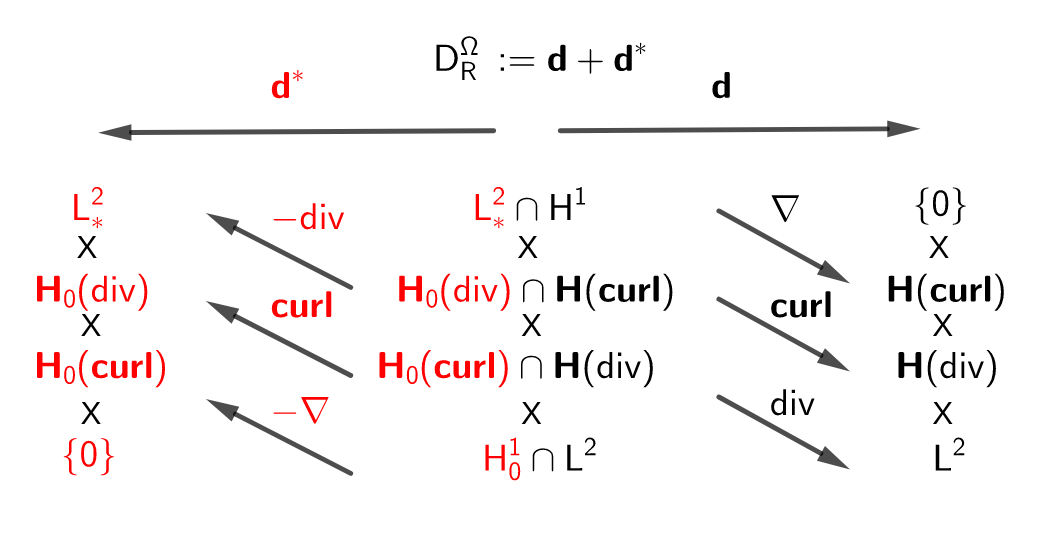
Figure 1: This diagram shows the mapping properties of the exterior derivatives and their Hilbert space adjoints corresponding to the functional analytic setting of [26] for problem (R) in $\Omega^{-}$. In the figure, the operators on the left-hand side are to be understood as the adjoint operators ${\color[rgb]{1,0,0}-\text{div}}=\nabla^{*}$, ${\color[rgb]{1,0,0}\mathbf{curl}}=\mathbf{curl}^{*}$ and ${\color[rgb]{1,0,0}-\nabla}=\text{div}^{*}$.

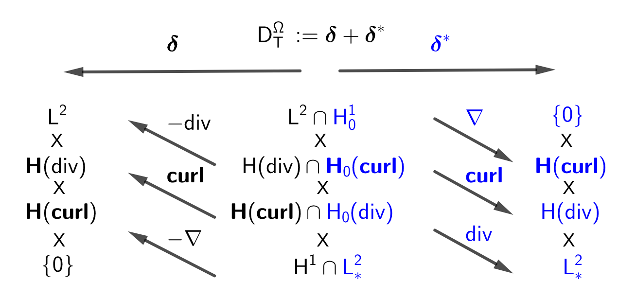
Figure 2: This diagram shows the mapping properties of the codifferentials and their Hilbert space adjoints corresponding to the functional analytic setting of [26] for problem (T) in $\Omega^{-}$. In the figure, the operators on the left-hand side are to be understood as the adjoint operators ${\color[rgb]{0,0,1}\nabla}=-\text{div}^{*}$, ${\color[rgb]{0,0,1}\mathbf{curl}}=\mathbf{curl}^{*}$ and ${\color[rgb]{0,0,1}\text{div}}=-\nabla$.

So unlike second-order operators, the Hodge–Dirac operator admits two distinct fundamental symmetric bilinear forms

(25a) $$\color[rgb]{0,0,1}\mathcal{A}_{\bm{\delta}}(\vec{\mathbf{U}},\vec{\mathbf{V}}) =\color[rgb]{0,0,1}\int_{\Omega}\bm{\delta}\vec{\mathbf{U}}\cdot\vec{\mathbf{V}}+\vec{\mathbf{U}}\cdot\bm{\delta}\vec{\mathbf{V}}\operatorname{d\!}\mathbf{x}, \vec{\mathbf{U}},\vec{\mathbf{V}}\in\mathbf{H}(\bm{\delta},\Omega),$$

(25b) $$\color[rgb]{1,0,0}\mathcal{A}_{\mathbf{d}}(\vec{\mathbf{U}},\vec{\mathbf{V}}) =\color[rgb]{1,0,0}\int_{\Omega}\mathbf{d}\vec{\mathbf{U}}\cdot\vec{\mathbf{V}}+\vec{\mathbf{U}}\cdot\mathbf{d}\vec{\mathbf{V}}\operatorname{d\!}\mathbf{x}, \vec{\mathbf{U}},\vec{\mathbf{V}}\in\mathbf{H}(\mathbf{d},\Omega),$$

that rest on an equal footing. They readily appear upon integrating by parts with Lemma 2.3 and they are involved in the first-order analogs of Green’s identities

(26a) $$\int_{\Omega^{\mp}}{\mathsf{D}\vec{\mathbf{U}}\cdot\vec{\mathbf{V}}} =\mathcal{A}_{\bm{\delta}}(\vec{\mathbf{U}},\vec{\mathbf{V}})\pm\llangle\gamma_{\mathsf{T}}\vec{\mathbf{U}},\gamma_{\mathsf{R}}\vec{\mathbf{V}}\rrangle_{\Gamma},$$

(26b) $$\int_{\Omega^{\mp}}{\mathsf{D}\vec{\mathbf{U}}\cdot\vec{\mathbf{V}}} =\mathcal{A}_{\mathbf{d}}(\vec{\mathbf{U}},\vec{\mathbf{V}})\mp\llangle\gamma_{\mathsf{T}}\vec{\mathbf{V}},\gamma_{\mathsf{R}}\vec{\mathbf{U}}\rrangle_{\Gamma},$$

which hold for all $\vec{\mathbf{U}},\vec{\mathbf{V}}\in\mathbf{H}(\mathsf{D},\Omega)$.

These identities lead to the variational problems:

(VT) $$\vec{\mathbf{U}}\in\mathbf{H}(\bm{\delta},\Omega)\,\mathrel{\mathop{\ordinarycolon}} \quad\color[rgb]{0,0,1}\mathcal{A}_{\bm{\delta}}(\vec{\mathbf{U}},\vec{\mathbf{V}}) =\color[rgb]{0,0,1}-\llangle\vec{\mathbf{b}},\gamma_{\mathsf{R}}\vec{\mathbf{V}}\rrangle_{\Gamma}, \forall\,\vec{\mathbf{V}}\in\mathbf{H}(\bm{\delta},\Omega),$$

and

(VR) $$\vec{\mathbf{U}}\in\mathbf{H}(\mathbf{d},\Omega)\,\mathrel{\mathop{\ordinarycolon}} \quad\color[rgb]{1,0,0}\mathcal{A}_{\mathbf{d}}(\vec{\mathbf{U}},\vec{\mathbf{V}}) =\color[rgb]{1,0,0}\llangle\vec{\mathbf{a}},\gamma_{\mathsf{T}}\vec{\mathbf{V}}\rrangle_{\Gamma}, \,\,\,\,\forall\,\vec{\mathbf{V}}\in\mathbf{H}(\mathbf{d},\Omega).$$

3.1 Compatibility conditions

Either from Green’s second formula for the Dirac operator (18) or the variational problems themselves, we see that the boundary values $\vec{\mathbf{b}}\in\mathcal{H}_{\mathsf{T}}$ and $\vec{\mathbf{a}}\in\mathcal{H}_{\mathsf{R}}$ must fulfill compatibility conditions. For the problems to admit solutions, we require that

(CCT) $${\color[rgb]{0,0,1}\llangle\vec{\mathbf{b}},\gamma_{\mathsf{R}}\vec{\mathbf{V}}\rrangle_{\Gamma}=\vec{\mathbf{0}},\qquad\qquad\forall\,\vec{\mathbf{V}}\in\mathfrak{H}_{T},}$$

and

(CCR) $${\color[rgb]{1,0,0}\llangle\vec{\mathbf{a}},\gamma_{\mathsf{T}}\vec{\mathbf{V}}\rrangle_{\Gamma}=\vec{\mathbf{0}},\qquad\qquad\forall\,\vec{\mathbf{V}}\in\mathfrak{H}_{R},}$$

where

(27a) $$\color[rgb]{0,0,1}\mathfrak{H}_{\mathsf{T}}(\Omega) \mathrel{\mathop{\ordinarycolon}}=\color[rgb]{0,0,1}\left\{\vec{\mathbf{V}}\in\mathbf{H}(\mathsf{D},\Omega)\mathrel{\mathop{\ordinarycolon}}\mathsf{D}\vec{\mathbf{V}}=0,\gamma_{\mathsf{T}}\vec{\mathbf{V}}=\vec{\mathbf{0}}\right\}$$

and

(27b) $$\color[rgb]{1,0,0}\mathfrak{H}_{\mathsf{R}}(\Omega) \color[rgb]{1,0,0}\mathrel{\mathop{\ordinarycolon}}=\{\vec{\mathbf{V}}\in\mathbf{H}(\mathsf{D},\Omega)\mathrel{\mathop{\ordinarycolon}}\mathsf{D}\vec{\mathbf{V}}=0,\gamma_{\mathsf{R}}\vec{\mathbf{V}}=\vec{\mathbf{0}}\}$$

are spaces of harmonic vector-fields. We refer to [2, 3, 1] and [26] for explanations on how these spaces exactly correspond to the nullspaces of the Hodge-Laplacian with natural and essential boundary conditions.

The fact that there are two distinct bilinear forms in the expressions (VT) and (VR) is one of the appealing use of the dual perspective involving the codifferential $\bm{\delta}$. It points to the symmetry presented in Remark 5.1 below, and it highlights the necessity of imposing compatibility conditions on the data. For example, we could alternatively formulate (T) as the variational problem

(28) $$\vec{\mathbf{U}}\in\mathbf{H}(\mathbf{d},\Omega)\,\quad\text{with}\quad\gamma_{\mathsf{T}}\vec{\mathbf{U}}=\vec{\mathbf{b}}\mathrel{\mathop{\ordinarycolon}} \quad\mathcal{A}_{\mathbf{d}}(\vec{\mathbf{U}},\vec{\mathbf{V}}) =0, \,\,\,\,\forall\,\vec{\mathbf{V}}\in\mathbf{H}_{0}(\mathbf{d},\Omega),$$

where $\mathbf{H}_{0}(\mathbf{d},\Omega)=H^{1}_{0}(\Omega)\times\mathbf{H}_{0}(\mathbf{curl},\Omega)\times\mathbf{H}_{0}(\text{div},\Omega)\times L^{2}(\Omega)$. But according to (18) the condition (CCT) must remain, and it now appears less obviously so when the type of boundary condition is essential. Anyway, in a formulation such as (28), one proceeds with a lifting of the boundary data and is left with the solvability of the problem

(29) $$\vec{\mathbf{U}}_{0}\in\mathbf{H}_{0}(\mathbf{d},\Omega)\,\mathrel{\mathop{\ordinarycolon}} \quad\mathcal{A}_{\mathbf{d}}(\vec{\mathbf{U}},\vec{\mathbf{V}}) =-\mathcal{A}_{\mathbf{d}}(\mathcal{E}_{\mathsf{T}}\vec{\mathbf{b}},\vec{\mathbf{V}}), \,\,\,\,\forall\,\vec{\mathbf{V}}\in\mathbf{H}_{0}(\mathbf{d},\Omega).$$

So the question of compatibly cannot be avoided: integrating by parts with the right-hand side evaluated at a nullspace element in $\mathfrak{H}_{\mathsf{T}}$ using (26b) leads to (CCT). We discuss in greater details the reason why the two boundary conditions can be formulated both as natural and essential in Remark 5.1.

3.2 Well-posedness

Since the bilinear form $\color[rgb]{0,0,1}\mathcal{A}_{\bm{\delta}}$ is associated with the self-adjoint operator $\color[rgb]{0,0,1}\mathsf{D}_{\mathsf{T}}$ obtained from the chain complex (24) and $\color[rgb]{1,0,0}\mathcal{A}_{\mathbf{d}}$ to the self-adjoint operator $\color[rgb]{1,0,0}\mathsf{D}_{\mathsf{R}}$ spawned by the cochain complex (20), they fit the framework of [26, Sec. 2]. The abstract inf-sup inequality supplied in [26, Thm. 6] applies to both bilinear forms and leads to well-posedness of the mixed variational problems:

(MVT) $$\begin{split}\color[rgb]{0,0,1}\mathcal{A}_{\bm{\delta}}(\vec{\mathbf{U}},\vec{\mathbf{V}})+\left(\vec{\mathbf{P}},\vec{\mathbf{V}}\right)_{\Omega}&\color[rgb]{0,0,1}=-\llangle\vec{\mathbf{b}},\gamma_{\mathsf{R}}\vec{\mathbf{V}}\rrangle_{\Gamma}\quad\qquad\forall\,\vec{\mathbf{V}}\in\mathbf{H}\left(\bm{\delta},\Omega^{-}\right),\\ \color[rgb]{0,0,1}\left(\vec{\mathbf{U}},\vec{\mathbf{W}}\right)_{\Omega}&\color[rgb]{0,0,1}=0\qquad\qquad\qquad\qquad\forall\,\vec{\mathbf{W}}\in\ker\mathsf{D}^{\Omega}_{\mathsf{T}},\end{split}$$

and

(MVR) $$\begin{split}\color[rgb]{1,0,0}\mathcal{A}_{\mathbf{d}}(\vec{\mathbf{U}},\vec{\mathbf{V}})+\left(\vec{\mathbf{Q}},\vec{\mathbf{V}}\right)_{\Omega}&\color[rgb]{1,0,0}=\llangle\vec{\mathbf{a}},\gamma_{\mathsf{T}}\vec{\mathbf{V}}\rrangle_{\Gamma}\quad\qquad\forall\,\vec{\mathbf{V}}\in\mathbf{H}\left(\mathbf{d},\Omega^{-}\right),\\ \color[rgb]{1,0,0}\left(\vec{\mathbf{U}},\vec{\mathbf{W}}\right)_{\Omega}&\color[rgb]{1,0,0}=0\quad\qquad\qquad\qquad\forall\,\vec{\mathbf{W}}\in\ker\mathsf{D}^{\Omega}_{\mathsf{R}},\end{split}$$

for unknown pairs $(\vec{\mathbf{U}},\vec{\mathbf{P}})\in\mathbf{H}(\bm{\delta},\Omega^{-})\times\ker\mathsf{D}_{\mathsf{T}}$ and $(\vec{\mathbf{U}},\vec{\mathbf{Q}})\in\mathbf{H}(\mathbf{d},\Omega^{-})\times\ker\mathsf{D}_{\mathsf{R}}$.

Consistency of the right-hand side in (VT) exactly corresponds to requiring that (CCT) holds for the given data $\vec{\mathbf{b}}\in\mathcal{H}_{\mathsf{T}}$, while (CCR) similarly guarantees consistency of the right-hand side in (VR). We conclude that if the compatibility conditions are satisfied, solutions to (VT) and (VR) in $\Omega^{-}$ are unique up to contributions of harmonic vector-fields in $\ker\mathsf{D}_{\mathsf{T}}$ and $\ker\mathsf{D}_{\mathsf{R}}$. Moreover, they continuously depend on the boundary data.

4 Representation formulas

We derive interior and exterior representation formulas for solutions of the Dirac equation. It is expressed through known boundary potentials, whose jump properties across $\Gamma$ are elaborated.

4.1 Fundamental solution

Convolution of a vector field $\vec{\mathbf{U}}\mathrel{\mathop{\ordinarycolon}}\mathbb{R}^{3}\rightarrow\mathbb{R}^{8}$ by a matrix-valued function $\mathsf{K}\mathrel{\mathop{\ordinarycolon}}\mathbb{R}^{3}\backslash\{\mathbf{0}\}\rightarrow\mathbb{R}^{8,8}$ possibly having a singularity at the $\mathbf{0}\in\mathbb{R}^{3}$ is defined, if the limit exists, as the Cauchy principal value

(30) $$\left(\mathsf{K}*\vec{\mathbf{U}}\right)\left(\mathbf{x}\right)\mathrel{\mathop{\ordinarycolon}}=\lim_{\epsilon\rightarrow 0}\int_{\mathbb{R}^{3}\backslash B_{\epsilon}(\mathbf{0})}\mathsf{K}(\mathbf{x}-\mathbf{y})\vec{\mathbf{U}}\left(\mathbf{y}\right)\operatorname{d\!}\mathbf{y}\in\mathbb{R}^{8},$$

where $B_{\epsilon}\left(\mathbf{0}\right)\subset\mathbb{R}^{3}$ is a ball of radius $\epsilon$ centered at the origin.

Let $G\mathrel{\mathop{\ordinarycolon}}\mathbb{R}^{3}\backslash\left\{\mathbf{0}\right\}\rightarrow\mathbb{R}$ be given by $G\left(\mathbf{z}\right)\mathrel{\mathop{\ordinarycolon}}=\left(4\pi\mathinner{\!\left\lvert\mathbf{z}\right\rvert}\right)^{-1}$, and set

(31) $$\mathsf{G}\left(\mathbf{z}\right)\mathrel{\mathop{\ordinarycolon}}=G\left(\mathbf{z}\right)\mathsf{I}_{8}\in\mathbb{R}^{8,8},\qquad\mathbf{z}\neq\mathbf{0},$$

where $\mathsf{I}_{8}$ is the identity matrix on $\mathbb{R}^{8}$. Then, define $\Phi\mathrel{\mathop{\ordinarycolon}}\mathbb{R}^{3}\backslash\{\mathbf{0}\}\rightarrow\mathbb{R}^{8,8}$ by applying the Dirac operator to the columns of $\mathsf{G}$ as

$$\Phi\left(\mathbf{z}\right)\mathrel{\mathop{\ordinarycolon}}=\begin{pmatrix}0&-\left(\nabla G\right)^{\top}\left(\mathbf{z}\right)&\mathbf{0}^{\top}&0\\ \left(\nabla G\right)\left(\mathbf{z}\right)&\mathbf{0}_{\,3\times 3}&\mathsf{A}_{3\times 3}(\mathbf{z})&\mathbf{0}\\ \mathbf{0}&\mathsf{A}_{3\times 3}(\mathbf{z})&\mathbf{0}_{\,3\times 3}&-\left(\nabla G\right)\left(\mathbf{z}\right)\\ 0&\mathbf{0}^{\top}&\left(\nabla G\right)^{\top}\left(\mathbf{z}\right)&0\end{pmatrix}\in\mathbb{R}^{8\times 8},\,\,\mathbf{z}\neq\mathbf{0},$$

where the anti-symmetric blocks

(32) $$\mathsf{A}_{3\times 3}(\mathbf{z})\mathrel{\mathop{\ordinarycolon}}=\begin{pmatrix}0&-\left(\partial_{3}G\right)\left(\mathbf{z}\right)&\left(\partial_{2}G\right)\left(\mathbf{z}\right)\\ \left(\partial_{3}G\right)\left(\mathbf{z}\right)&0&-\left(\partial_{1}G\right)\left(\mathbf{z}\right)\\ -\left(\partial_{2}G\right)\left(\mathbf{z}\right)&\left(\partial_{1}G\right)\left(\mathbf{z}\right)&0\end{pmatrix}\in\mathbb{R}^{3\times 3},\qquad\mathbf{z}\neq\mathbf{0},$$

are associated with the curl operator.

Lemma 4.1.

For $\mathbf{z}\neq\mathbf{0}$,

(33) $$\Phi\left(-\mathbf{z}\right)=-\Phi\left(\mathbf{z}\right) \Phi\left(\mathbf{z}\right)\vec{\mathbf{U}}\cdot\vec{\mathbf{V}}=-\vec{\mathbf{U}}\cdot\Phi\left(\mathbf{z}\right)\vec{\mathbf{V}}$$ and

for all $\vec{\mathbf{U}},\vec{\mathbf{V}}\in\mathbb{R}^{8}$.

Proof 4.2.

Let $\mathsf{s}\mathrel{\mathop{\ordinarycolon}}\mathbb{R}^{3}\rightarrow\mathbb{R}^{3}$ be the sign flip operation $\mathsf{s}(\mathbf{z})=-\mathbf{z}$. For the fist identity, we simply rely on the fact that $G\left(\mathbf{x}\right)=G\left(\,\mathinner{\!\left\lvert\mathbf{x}\right\rvert}\right)$ to verify that for any $\vec{\mathbf{U}}\in\mathbb{R}^{8}$,

(34) $$\Phi\left(-\mathbf{z}\right)\vec{\mathbf{U}}=\mathsf{D}\left(\mathsf{G}\vec{\mathbf{U}}\right)\Big{|}_{\mathsf{s}\left(\mathbf{z}\right)}=-\mathsf{D}_{\mathbf{x}}\left(\mathsf{G}\left(\sf{s}\left(\mathbf{x}\right)\right)\vec{\mathbf{U}}\right)\Big{|}_{\mathbf{x}=\mathbf{z}}\\ =-\mathsf{D}_{\mathbf{x}}\left(G\left(\sf{s}\left(\mathbf{x}\right)\right)\vec{\mathbf{U}}\right)\Big{|}_{\mathbf{x}=\mathbf{z}}=-\mathsf{D}_{\mathbf{x}}\left(G\left(\mathbf{x}\right)\vec{\mathbf{U}}\right)\Big{|}_{\mathbf{x}=\mathbf{z}}=-\Phi\left(\mathbf{z}\right)\vec{\mathbf{U}}.$$

The second identity is clear by definition.

This lemma allows to extend the domain of the Newton-type potential

$$\mathsf{N}\mathrel{\mathop{\ordinarycolon}}C_{0}^{\infty}(\mathbb{R}^{3})^{8} \rightarrow C^{\infty}(\mathbb{R}^{3})^{8}$$

$$\vec{\mathbf{U}} \mapsto\Phi*\vec{\mathbf{U}}$$

to distributions.

Lemma 4.3.

For all $\vec{\mathbf{U}},\vec{\mathbf{V}}\in C^{\infty}_{0}(\mathbb{R}^{3})^{8}$,

(35) $$\left(\mathsf{N}\,\vec{\mathbf{U}},\vec{\mathbf{V}}\right)=\left(\vec{\mathbf{U}},\mathsf{N}\,\vec{\mathbf{V}}\right).$$

Proof 4.4.

Using Lemma 4.1, we can change the order of integration using Fubini’s theorem and evaluate

(36) $$\left(\mathsf{N}\vec{\mathbf{U}},\vec{\mathbf{V}}\right) =\int_{\mathbb{R}^{3}}\int_{\mathbb{R}^{3}}\Phi\left(\mathbf{x}-\mathbf{y}\right)\vec{\mathbf{U}}\left(\mathbf{y}\right)\cdot\vec{\mathbf{V}}\left(\mathbf{x}\right)\operatorname{d\!}\mathbf{x}\operatorname{d\!}\mathbf{y}$$

(37) $$=\int_{\mathbb{R}^{3}}\int_{\mathbb{R}^{3}}\vec{\mathbf{U}}\left(\mathbf{y}\right)\cdot\Phi\left(\mathbf{y}-\mathbf{x}\right)\vec{\mathbf{V}}\left(\mathbf{x}\right)\operatorname{d\!}\mathbf{x}\operatorname{d\!}\mathbf{y}$$

(38) $$=\int_{\mathbb{R}^{3}}\vec{\mathbf{U}}\left(\mathbf{y}\right)\cdot\int_{\mathbb{R}^{3}}\Phi\left(\mathbf{y}-\mathbf{x}\right)\vec{\mathbf{V}}\left(\mathbf{x}\right)\operatorname{d\!}\mathbf{x}\operatorname{d\!}\mathbf{y}$$

(39) $$=\left(\vec{\mathbf{U}},\mathsf{N}\,\vec{\mathbf{V}}\right).$$

Remark 4.5.

Lemma 4.3 reflects the fact that the Dirac operator is symmetric as an unbounded operator on $(L^{2}(\mathbb{R}^{3}))^{8}$.

The extension

(40) $$\mathsf{N}\mathrel{\mathop{\ordinarycolon}}(C^{\infty}(\mathbb{R}^{3})^{8})^{\prime}\rightarrow(C^{\infty}_{0}(\mathbb{R}^{3})^{8})^{\prime}$$

is obtained as in [37, Sec. 3.1.1] via dual mapping by defining the action of the distribution $\mathsf{N}\vec{\mathbf{U}}\in(C^{\infty}_{0}(\mathbb{R}^{3})^{8})^{\prime}$ on $\vec{\mathbf{V}}\in C^{\infty}_{0}(\mathbb{R}^{3})^{8}$ as

(41) $$\langle\mathsf{N}\,\vec{\mathbf{U}},\vec{\mathbf{V}}\rangle\mathrel{\mathop{\ordinarycolon}}=\langle\vec{\mathbf{U}},\mathsf{N}\,\vec{\mathbf{V}}\rangle.$$

Proposition 4.6 (Fundamental solution).

For all compactly supported distributions $\vec{\mathbf{U}}\in(C^{\infty}(\mathbb{R}^{3})^{8})^{\prime}$,

(42) $$\mathsf{N}\,\mathsf{D}\,\vec{\mathbf{U}}=\vec{\mathbf{U}}=\mathsf{D}\,\mathsf{N}\,\vec{\mathbf{U}}$$

holds in $(C^{\infty}_{0}(\mathbb{R}^{3})^{8})^{\prime}$.

Proof 4.7.

We first show that for $\vec{\mathbf{U}}\in(C^{\infty}(\mathbb{R}^{3})^{8})^{\prime}$,

(43) $$\langle\mathsf{N}\,\mathsf{D}\vec{\mathbf{U}},\vec{\mathbf{V}}\rangle=\langle\vec{\mathbf{U}},\vec{\mathbf{V}}\rangle$$

for all $\vec{\mathbf{V}}\in C^{\infty}_{0}(\mathbb{R}^{3})^{8}$.

The argument is inspired by the proof of [18, Thm.1]. Let $\mathbf{e}_{i}\in\mathbb{R}^{3}$ be the vector with $1$ at the i-th entry and zeros elsewhere, $i=1,2,3$. Since

(44) $$\mathsf{N}\vec{\mathbf{V}}=\int_{\mathbb{R}^{3}}\Phi\left(\mathbf{x}-\mathbf{y}\right)\vec{\mathbf{V}}\left(\mathbf{y}\right)\operatorname{d\!}\mathbf{y}=\int_{\mathbb{R}^{3}}\Phi\left(\mathbf{y}\right)\vec{\mathbf{V}}\left(\mathbf{x}-\mathbf{y}\right)\operatorname{d\!}\mathbf{y},$$

we have

(45) $$\frac{\mathsf{N}\vec{\mathbf{V}}\left(\mathbf{x}+h\mathbf{e}_{i}\right)-\mathsf{N}\vec{\mathbf{V}}\left(\mathbf{x}\right)}{h}=\int_{\mathbb{R}^{3}}\Phi\left(\mathbf{y}\right)\frac{\vec{\mathbf{V}}\left(\mathbf{x}+h\mathbf{e}_{i}-\mathbf{y}\right)-\vec{\mathbf{V}}\left(\mathbf{x}-\mathbf{y}\right)}{h}\operatorname{d\!}\mathbf{y}.$$

Hence,

(46) $$\mathsf{D}_{\mathbf{x}}\mathsf{N}\vec{\mathbf{V}}\left(\mathbf{x}\right)=\int_{\mathbb{R}^{3}}\Phi\left(\mathbf{y}\right)\mathsf{D}\vec{\mathbf{V}}\left(\mathbf{x}-\mathbf{y}\right)\operatorname{d\!}\mathbf{y},$$

because the assumption that $\vec{\mathbf{V}}$ is smooth and compactly supported guarantees that

(47) $$\frac{\vec{\mathbf{V}}\left(\mathbf{x}+h\mathbf{e}_{i}-\mathbf{y}\right)-\vec{\mathbf{V}}\left(\mathbf{x}-\mathbf{y}\right)}{h}\rightarrow\frac{\partial}{\partial\mathbf{x}_{i}}\vec{\mathbf{V}}\left(\mathbf{x}-\mathbf{y}\right)$$

uniformly for $h\rightarrow 0$. The main idea is to isolate $\Phi$’s singularity at the origin by splitting the right hand side of Eq. 46 into two integrals as

(48) $$\mathsf{D}_{\mathbf{x}}\mathsf{N}\vec{\mathbf{V}}\left(\mathbf{x}\right)=\underbrace{\int_{B_{\epsilon}\left(\mathbf{0}\right)}\Phi\left(\mathbf{y}\right)\mathsf{D}\vec{\mathbf{V}}\left(\mathbf{x}-\mathbf{y}\right)\operatorname{d\!}\mathbf{y}}_{I_{\epsilon}}+\underbrace{\int_{\mathbb{R}^{3}\backslash B_{\epsilon}\left(\mathbf{0}\right)}\Phi\left(\mathbf{y}\right)\mathsf{D}\vec{\mathbf{V}}\left(\mathbf{x}-\mathbf{y}\right)\operatorname{d\!}\mathbf{y}}_{J_{\epsilon}}$$

whose limits as $\epsilon\rightarrow 0$ we can control.

The main difficulty is that we cannot readily mimic the standard proof commonly given for the Poisson equation, because the integration by parts formula supplied for the product of two vectors by Eq. 18 is not applicable to the matrix–vector multiplication involved in the integrands of Eq. 48. The analysis of

(49) $$\Phi\left(\mathbf{y}\right)\mathsf{D}\vec{\mathbf{V}}\left(\mathbf{x}-\mathbf{y}\right)=\\ \begin{pmatrix}-{\color[rgb]{0.82,0.1,0.26}\nabla G\left(\mathbf{y}\right)\cdot\nabla V_{0}\left(\mathbf{x}-\mathbf{y}\right)}-{\color[rgb]{0.0,0.5,0.0}\nabla G\left(\mathbf{y}\right)\cdot\mathbf{curl}\,\mathbf{V}_{1}\left(\mathbf{x}-\mathbf{y}\right)}\\ -{\color[rgb]{1,.5,0}\text{div}\,\mathbf{V}_{1}\left(\mathbf{x}-\mathbf{y}\right)\nabla G\left(\mathbf{y}\right)}-{\color[rgb]{.5,0,.5}\nabla G\left(\mathbf{y}\right)\times\nabla V_{3}\left(\mathbf{x}-\mathbf{y}\right)}+{\color[rgb]{0,.5,.5}\nabla G\left(\mathbf{y}\right)\times\mathbf{curl}\,\mathbf{V}_{1}\left(\mathbf{x}-\mathbf{y}\right)}\\ -{\color[rgb]{.5,0,.5}\nabla G\left(\mathbf{y}\right)\times\nabla V_{0}\left(\mathbf{x}-\mathbf{y}\right)}+{\color[rgb]{0,.5,.5}\nabla G\left(\mathbf{y}\right)\times\mathbf{curl}\,\mathbf{V}_{2}\left(\mathbf{x}-\mathbf{y}\right)}-{\color[rgb]{1,.5,0}\text{div}\,\mathbf{V}_{2}\left(\mathbf{x}-\mathbf{y}\right)\nabla G\left(\mathbf{y}\right)}\\ -{\color[rgb]{0.82,0.1,0.26}\nabla G\left(\mathbf{y}\right)\cdot\nabla V_{3}\left(\mathbf{x}-\mathbf{y}\right)}+{\color[rgb]{0.0,0.5,0.0}\nabla G\left(\mathbf{y}\right)\cdot\mathbf{curl}\,\mathbf{V}_{2}\left(\mathbf{x}-\mathbf{y}\right)}\end{pmatrix}$$

is carried out component-wise.

There are five different types of terms whose limit need to be investigated. Let $\mathbf{V}\in(C^{\infty}_{0}(\mathbb{R}^{3}))^{3}$ and $V\in C^{\infty}_{0}(\mathbb{R}^{3})$ be arbitrary fields. To ease the reading, we write $V_{\mathbf{x}}(\mathbf{y})\mathrel{\mathop{\ordinarycolon}}=V(\mathbf{x}-\mathbf{y})$ and $\mathbf{V}_{\mathbf{x}}(\mathbf{y})\mathrel{\mathop{\ordinarycolon}}=\mathbf{V}(\mathbf{x}-\mathbf{y})$ . We denote by $\mathbf{n}_{\epsilon}$ the unit normal vector field pointing towards the interior of $B_{\epsilon}\left(\mathbf{0}\right)$.

Integrating by parts using that $\Delta G=0$ in $\mathbb{R}^{3}\backslash\left(\mathbf{0}\right)$ and $\mathbf{curl}\circ\nabla\equiv\mathbf{0}$, we find that

(50) $$\int_{\mathbb{R}^{3}\backslash B_{\epsilon}\left(\mathbf{0}\right)}{\color[rgb]{0.82,0.1,0.26}\nabla G\left(\mathbf{y}\right)\cdot\nabla V\left(\mathbf{x}-\mathbf{y}\right)}\operatorname{d\!}\mathbf{y}=\int_{\partial B_{\epsilon}\left(\mathbf{0}\right)}\nabla G\left(\mathbf{y}\right)\cdot\mathbf{n}_{\epsilon}\left(\mathbf{y}\right)V\left(\mathbf{x}-\mathbf{y}\right)\operatorname{d\!}\sigma\left(\mathbf{y}\right)\\ =\frac{1}{4\pi}\int_{\partial B_{\epsilon}\left(\mathbf{0}\right)}\frac{V\left(\mathbf{x}-\mathbf{y}\right)}{\mathinner{\!\left\lvert\mathbf{y}\right\rvert}^{3}}\left(-\mathbf{y}\cdot\frac{\mathbf{y}}{\mathinner{\!\left\lvert\mathbf{y}\right\rvert}}\right)\operatorname{d\!}\sigma\left(\mathbf{y}\right)=-\frac{1}{4\pi\epsilon^{2}}\int_{\partial B_{\epsilon}\left(\mathbf{0}\right)}V\left(\mathbf{x}-\mathbf{y}\right)\operatorname{d\!}\sigma\left(\mathbf{y}\right)\\ =-\mathchoice{{\vbox{\hbox{$\textstyle-$ }}\kern-7.83337pt}}{{\vbox{\hbox{$\scriptstyle-$ }}\kern-5.90005pt}}{{\vbox{\hbox{$\scriptscriptstyle-$ }}\kern-4.75003pt}}{{\vbox{\hbox{$\scriptscriptstyle-$ }}\kern-4.25003pt}}\!\int_{\partial B_{\epsilon}\left(\mathbf{x}\right)}V\left(\mathbf{y}\right)\operatorname{d\!}\sigma\left(\mathbf{y}\right)\xrightarrow[\epsilon\rightarrow 0]{}-V\left(\mathbf{x}\right)$$

and

(51) $$\int_{\mathbb{R}^{3}\backslash B_{\epsilon}\left(\mathbf{0}\right)}{\color[rgb]{0.0,0.5,0.0}\nabla G\left(\mathbf{y}\right)\cdot\mathbf{curl}\,\mathbf{V}\left(\mathbf{x}-\mathbf{y}\right)}\operatorname{d\!}\mathbf{y}\\ =-\int_{\partial B_{\epsilon}\left(\mathbf{0}\right)}\left(\nabla G\left(\mathbf{y}\right)\times\mathbf{n}_{\epsilon}\left(\mathbf{y}\right)\right)\cdot\mathbf{V}\left(\mathbf{x}-\mathbf{y}\right)\operatorname{d\!}\sigma\left(\mathbf{y}\right)\\ =-\frac{1}{4\pi\epsilon^{4}}\int_{\partial B_{\epsilon}\left(\mathbf{0}\right)}\left(\mathbf{y}\times\mathbf{y}\right)\cdot\mathbf{V}\left(\mathbf{x}-\mathbf{y}\right)\operatorname{d\!}\sigma\left(\mathbf{y}\right)=0.$$

Similarly, integrating by parts component-wise yields

(52) $$\int_{\mathbb{R}^{3}\backslash B_{\epsilon}\left(\mathbf{0}\right)}{\color[rgb]{.5,0,.5}\nabla G\left(\mathbf{y}\right)\times\nabla V_{\mathbf{x}}(\mathbf{y})}\operatorname{d\!}\mathbf{y}\\ =\int_{\mathbb{R}^{3}\backslash B_{\epsilon}\left(\mathbf{0}\right)}\begin{pmatrix}\partial_{2}G\left(\mathbf{y}\right)\partial_{3}V_{\mathbf{x}}(\mathbf{y})-\partial_{3}G\left(\mathbf{y}\right)\partial_{2}V_{\mathbf{x}}(\mathbf{y})\\ \partial_{3}G\left(\mathbf{y}\right)\partial_{1}V_{\mathbf{x}}(\mathbf{y})-\partial_{1}G\left(\mathbf{y}\right)\partial_{3}V_{\mathbf{x}}(\mathbf{y})\\ \partial_{1}G\left(\mathbf{y}\right)\partial_{2}V_{\mathbf{x}}(\mathbf{y})-\partial_{2}G\left(\mathbf{y}\right)\partial_{1}V_{\mathbf{x}}(\mathbf{y})\end{pmatrix}\operatorname{d\!}\mathbf{y}\\ =\int_{\mathbb{R}^{3}\backslash B_{\epsilon}\left(\mathbf{0}\right)}\begin{pmatrix}G\left(\mathbf{y}\right)\partial_{2}\partial_{3}V_{\mathbf{x}}(\mathbf{y})-G\left(\mathbf{y}\right)\partial_{3}\partial_{2}V_{\mathbf{x}}(\mathbf{y})\\ G\left(\mathbf{y}\right)\partial_{3}\partial_{1}V_{\mathbf{x}}(\mathbf{y})-G\left(\mathbf{y}\right)\partial_{1}\partial_{3}V_{\mathbf{x}}(\mathbf{y})\\ G\left(\mathbf{y}\right)\partial_{1}\partial_{2}V_{\mathbf{x}}(\mathbf{y})-G\left(\mathbf{y}\right)\partial_{2}\partial_{1}V_{\mathbf{x}}(\mathbf{y})\end{pmatrix}\operatorname{d\!}\mathbf{y}\\ +\int_{\partial B_{\epsilon}\left(\mathbf{0}\right)}\begin{pmatrix}-\left(\mathbf{n}_{\epsilon}\right)_{2}\left(\mathbf{y}\right)G\left(\mathbf{y}\right)\partial_{3}V_{\mathbf{x}}(\mathbf{y})+\left(\mathbf{n}_{\epsilon}\right)_{3}\left(\mathbf{y}\right)G\left(\mathbf{y}\right)\partial_{2}V_{\mathbf{x}}(\mathbf{y})\\ -\left(\mathbf{n}_{\epsilon}\right)_{2}\left(\mathbf{y}\right)G\left(\mathbf{y}\right)\partial_{1}V_{\mathbf{x}}(\mathbf{y})+\left(\mathbf{n}_{\epsilon}\right)_{1}\left(\mathbf{y}\right)G\left(\mathbf{y}\right)\partial_{3}V_{\mathbf{x}}(\mathbf{y})\\ -\left(\mathbf{n}_{\epsilon}\right)_{1}\left(\mathbf{y}\right)G\left(\mathbf{y}\right)\partial_{2}V_{\mathbf{x}}(\mathbf{y})+\left(\mathbf{n}_{\epsilon}\right)_{2}\left(\mathbf{y}\right)G\left(\mathbf{y}\right)\partial_{1}V_{\mathbf{x}}(\mathbf{y})\end{pmatrix}\operatorname{d\!}\mathbf{y}.$$

Since $V$ is smooth everywhere in $\mathbb{R}^{3}$, partial derivatives commute and the volume integral vanishes, leading to

(53) $$\int_{\mathbb{R}^{3}\backslash B_{\epsilon}\left(\mathbf{0}\right)}{\color[rgb]{.5,0,.5}\nabla G\left(\mathbf{y}\right)\times\nabla V_{\mathbf{x}}(\mathbf{y})}\operatorname{d\!}\mathbf{y}=-\int_{\partial B_{\epsilon}\left(\mathbf{0}\right)}G\left(\mathbf{y}\right)\mathbf{n}_{\epsilon}\left(\mathbf{y}\right)\times\nabla V_{\mathbf{x}}(\mathbf{y})\operatorname{d\!}\sigma\left(\mathbf{y}\right).$$

This integral vanishes under the limit $\epsilon\rightarrow 0$, because

(54) $$\sup_{\mathbf{x}\in\mathbb{R}^{3}}\,\mathinner{\!\left\lvert\int_{\partial B_{\epsilon}\left(\mathbf{0}\right)}G\left(\mathbf{y}\right)\mathbf{n}_{\epsilon}\left(\mathbf{y}\right)\times\nabla V\left(\mathbf{x}-\mathbf{y}\right)\operatorname{d\!}\sigma\left(\mathbf{y}\right)\right\rvert}\\ \leq\mathinner{\!\left\lVert\nabla V\right\rVert}_{\infty}\int_{\partial B_{\epsilon}\left(\mathbf{0}\right)}\mathinner{\!\left\lvert G\left(\mathbf{y}\right)\right\rvert}\operatorname{d\!}\sigma\left(\mathbf{y}\right)=\mathcal{O}\left(\epsilon\right).$$

Moving on to the next term, one eventually obtains from similar calculations that

(55) $$\int_{\mathbb{R}^{3}\backslash B_{\epsilon}\left(\mathbf{0}\right)}{\color[rgb]{0,.5,.5}\nabla G\left(\mathbf{y}\right)\times\mathbf{curl}\,\mathbf{V}_{\mathbf{x}}(\mathbf{y})}\operatorname{d\!}\mathbf{y}=\int_{\mathbb{R}^{3}\backslash B_{\epsilon}\left(\mathbf{0}\right)}G\left(\mathbf{y}\right)\mathbf{curl}\,\mathbf{curl}\,\mathbf{V}_{\mathbf{x}}(\mathbf{y})\operatorname{d\!}\mathbf{y}\\ +\int_{\partial B_{\epsilon}\left(\mathbf{0}\right)}G\left(\mathbf{y}\right)\left(\mathbf{curl}\,\mathbf{V}_{\mathbf{x}}(\mathbf{y})\times\mathbf{n}_{\epsilon}\left(\mathbf{y}\right)\right)\operatorname{d\!}\sigma\left(\mathbf{y}\right).$$

Since $\mathinner{\!\left\lVert\mathbf{curl}\,\mathbf{V}\right\rVert}_{\infty}<\infty$, the boundary integral on the right hand side vanishes under the limit by repeating the argument of Eq. 54. Finally, commuting partial derivatives after integrating by parts also yields

(56) $$\int_{\mathbb{R}^{3}\backslash B_{\epsilon}\left(\mathbf{0}\right)}{\color[rgb]{1,.5,0}\text{div}\,\mathbf{V}\left(\mathbf{x}-\mathbf{y}\right)\nabla G\left(\mathbf{y}\right)}\operatorname{d\!}\mathbf{y}\\ =\int_{\mathbb{R}^{3}\backslash B_{\epsilon}\left(\mathbf{0}\right)}G\left(\mathbf{y}\right)\nabla\text{div}\mathbf{V}\left(\mathbf{x}-\mathbf{y}\right)-\int_{\partial B_{\epsilon}\left(\mathbf{0}\right)}G\left(\mathbf{y}\right)\text{div}\mathbf{V}\left(\mathbf{x}-\mathbf{y}\right)\mathbf{n}_{\epsilon}\left(\mathbf{y}\right)\operatorname{d\!}\sigma\left(\mathbf{y}\right)$$

Putting the two previous calculations together, we find that

(57) $$\lim_{\epsilon\rightarrow 0}\int_{\mathbb{R}^{3}\backslash B_{\epsilon}\left(\mathbf{0}\right)}{\color[rgb]{0,.5,.5}\nabla G\left(\mathbf{y}\right)\times\mathbf{curl}\,\mathbf{V}\left(\mathbf{x}-\mathbf{y}\right)}-{\color[rgb]{1,.5,0}\text{div}\,\mathbf{V}\left(\mathbf{x}-\mathbf{y}\right)\nabla G\left(\mathbf{y}\right)}\operatorname{d\!}\mathbf{y}\\ =-\lim_{\epsilon\rightarrow 0}\int_{\mathbb{R}^{3}\backslash B_{\epsilon}\left(\mathbf{0}\right)}G\left(\mathbf{y}\right)\bm{\Delta}\mathbf{V}\left(\mathbf{x}-\mathbf{y}\right)\operatorname{d\!}\mathbf{y}=\mathbf{V}\left(\mathbf{x}\right),$$

where we recognized the vector (Hodge-) Laplace operator $-\bm{\Delta}\equiv\mathbf{curl}\,\mathbf{curl}-\nabla\,\text{div}$.

We have found that $J_{\epsilon}\longrightarrow\vec{\mathbf{V}}\left(\mathbf{x}\right)$ as $\epsilon\rightarrow 0$. Meanwhile,

(58) $$\mathinner{\!\left\lVert I_{\epsilon}\right\rVert}_{\infty}\leq\mathinner{\!\left\lVert\mathsf{D}\vec{\mathbf{V}}\right\rVert}_{\infty}\int_{B_{\epsilon}\left(\mathbf{0}\right)}\mathinner{\!\left\lVert\Phi\right\rVert}_{\infty}\operatorname{d\!}\mathbf{y}=\mathcal{O}\left(\int_{B_{\epsilon}\left(\mathbf{0}\right)}\mathinner{\!\left\lVert\nabla G\right\rVert}_{\infty}\operatorname{d\!}\mathbf{y}\right)=\mathcal{O}\left(\epsilon\right).$$

The calculations for $\vec{\mathbf{U}}=\mathsf{D}\,\mathsf{N}\,\vec{\mathbf{U}}$ follow similarly starting from (46).

In light of Proposition 4.6, we say that the kernel $\Phi$ of $\mathsf{N}$ is a fundamental solution for the Dirac operator.

4.2 Surface potentials

Adopting the perspective on first-kind boundary integral operators from [16], [32], [37] and [14]—in the later works for the study of second-order elliptic operators—for the first-order Dirac operator, we define the surface potentials

(59) $$\mathcal{L}_{\mathsf{T}}\left(\vec{\mathbf{a}}\right) \mathrel{\mathop{\ordinarycolon}}=\mathsf{N}\left(\gamma_{\mathsf{T}}^{\prime}\vec{\mathbf{a}}\right), \forall\,\vec{\mathbf{a}}=\left(\mathcal{a}_{0},\mathbf{a}_{1},a_{2}\right)\in\mathcal{H}_{\mathsf{R}},$$

(60) $$\mathcal{L}_{\mathsf{R}}(\vec{\mathbf{b}}) \mathrel{\mathop{\ordinarycolon}}=-\mathsf{N}\left(\gamma_{\mathsf{R}}^{\prime}\vec{\mathbf{b}}\right), \forall\,\vec{\mathbf{b}}=\left(b_{0},\mathbf{b}_{1},\mathcal{b}_{2}\right)\in\mathcal{H}_{\mathsf{T}},$$

where the mappings $\gamma_{\mathsf{T}}^{\prime}\mathrel{\mathop{\ordinarycolon}}\mathcal{H}_{\mathsf{R}}=\mathcal{H}_{\mathsf{T}}^{\prime}\rightarrow\mathbf{H}_{\text{loc}}(\mathsf{D},\mathbb{R}^{3}\backslash\overline{\Omega})^{\prime}$ and $\gamma_{\mathsf{R}}^{\prime}\mathrel{\mathop{\ordinarycolon}}\mathcal{H}_{\mathsf{T}}=\mathcal{H}_{\mathsf{R}}^{\prime}\rightarrow\mathbf{H}_{\text{loc}}(\mathsf{D},\mathbb{R}^{3}\backslash\overline{\Omega})^{\prime}$ are adjoint to the trace operators $\gamma_{\mathsf{T}}$ and $\gamma_{\mathsf{R}}$ defined in (13).

It will be convenient to denote by $\Phi_{\mathbf{x}}$ the map $\mathbf{y}\mapsto\Phi\left(\mathbf{x}-\mathbf{y}\right)$. Let $\vec{\mathbf{E}}_{j}\in\mathbb{R}^{8}$ denote the constant vector with $1$ at the $j$-th entry and zeros elsewhere, $j=1,...,8$. Similarly for $\mathbf{E}_{k}\in\mathbb{R}^{3}$, $k=1,2,3$.

Adapting the calculations found in [14, Sec. 4.2], we will establish integral representation formulas for these potentials by splitting the pairings into their components.

Lemma 4.8.

Given $\vec{\mathbf{a}}\in\mathcal{H}_{\mathsf{R}}$ and $\vec{\mathbf{b}}\in\mathcal{H}_{\mathsf{T}}$, it holds for $\mathbf{x}\in\Omega\backslash\Gamma$ that

(61a) $$\mathcal{L}_{\mathsf{T}}\left(\vec{\mathbf{a}}\right)\left(\mathbf{x}\right)\cdot\vec{\mathbf{E}}_{j} =-\llangle\vec{\mathbf{a}}\,,\,\gamma^{-}_{\mathsf{T}}\left(\Phi_{\mathbf{x}}\,\vec{\mathbf{E}}_{j}\right)\rrangle_{\Gamma},$$

(61b) $$\mathcal{L}_{\mathsf{R}}(\vec{\mathbf{b}})\left(\mathbf{x}\right)\cdot\vec{\mathbf{E}}_{j} =\llangle\vec{\mathbf{b}}\,,\,\gamma^{-}_{\mathsf{R}}\left(\Phi_{\mathbf{x}}\,\vec{\mathbf{E}}_{j}\right)\rrangle_{\Gamma}.$$

Proof 4.9.

Let $V\in C^{\infty}_{0}(\mathbb{R}^{3})$ and suppose that $\vec{\mathbf{a}}$ is the trace of a smooth $8$-dimensional vector-field. Using Fubini’s theorem and the fact that $\Phi$ is smooth away from the origin,

(62) $$\langle\mathsf{N}\left(\gamma_{\mathsf{T}}^{\prime}\vec{\mathbf{a}}\right),\,V\vec{\mathbf{E}}_{j}\rangle_{\mathbb{R}^{3}} =\llangle\vec{\mathbf{a}},\gamma_{\mathsf{T}}\mathsf{N}\left(V\vec{\mathbf{E}}_{j}\right)\rrangle_{\Gamma}$$

(63) $$=\int_{\Gamma}\vec{\mathbf{a}}\left(\mathbf{y}\right)\cdot\gamma_{\mathsf{T}}\int_{\mathbb{R}^{3}}\Phi\left(\mathbf{y}-\mathbf{x}\right)V\left(\mathbf{x}\right)\vec{\mathbf{E}}_{j}\left(\mathbf{x}\right)\operatorname{d\!}\mathbf{x}\operatorname{d\!}\sigma\left(\mathbf{y}\right)$$

(64) $$\stackrel{{\scriptstyle\mathclap{\mbox{($*$)}}}}{{=}}-\int_{\mathbb{R}^{3}}V\left(\mathbf{x}\right)\left(\int_{\Gamma}\vec{\mathbf{a}}\left(\mathbf{y}\right)\cdot\gamma_{\mathsf{T}}\Phi{\left(\mathbf{x}-\mathbf{y}\right)}\vec{\mathbf{E}}_{j}\operatorname{d\!}\sigma\left(\mathbf{y}\right)\right)\operatorname{d\!}\mathbf{x},$$

where the sign was obtained in ($*$) thanks to Lemma 4.1. The integrals on the right-hand side of (64) can be extended to duality pairings by a standard density argument exploiting Lemma 2.1.

Similar calculations can be carried out for $\mathcal{L}_{\mathsf{R}}$.

In particular,

(65) $$\Phi_{\mathbf{x}}\left(\mathbf{y}\right)\,\vec{\mathbf{E}}_{1} =\begin{pmatrix}0\\ \nabla G\left(\mathbf{x}-\mathbf{y}\right)\\ \mathbf{0}\\ 0\end{pmatrix}, \Phi_{\mathbf{x}}\left(\mathbf{y}\right)\,\vec{\mathbf{E}}_{8} =\begin{pmatrix}0\\ \mathbf{0}\\ -\nabla G\left(\mathbf{x}-\mathbf{y}\right)\\ 0\end{pmatrix},$$

(66) $$\Phi_{\mathbf{x}}\left(\mathbf{y}\right)\,\vec{\mathbf{E}}_{i} =\begin{pmatrix}-\frac{\partial}{\partial\mathbf{z}_{\mu(i)}}G\left(\mathbf{z}\right)\,\\ \mathbf{0}\\ \nabla G\left(\mathbf{z}\right)\times\mathbf{E}_{\mu\left(i\right)}\\ 0\end{pmatrix}\Big{|}_{\mathbf{z}=\mathbf{x}-\mathbf{y}}, \Phi_{\mathbf{x}}\left(\mathbf{y}\right)\,\vec{\mathbf{E}}_{k} =\begin{pmatrix}0\\ \nabla G\left(\mathbf{z}\right)\times\mathbf{E}_{\nu\left(k\right)}\\ \mathbf{0}\\ \frac{\partial}{\partial\mathbf{z}_{\nu(k)}}G\left(\mathbf{z}\right)\,\end{pmatrix}\Big{|}_{\mathbf{z}=\mathbf{x}-\mathbf{y}},$$

for $i=2,3,4$, $k=5,6,7$, $\mu\left(i\right)=i-1$ and $\nu\left(k\right)=k-4$.

Therefore, we can evaluate

(67a) $$\mathcal{L}_{\mathsf{T}}\left(\vec{\mathbf{a}}\right)\left(\mathbf{x}\right)\cdot\vec{\mathbf{E}}_{1} =-\int_{\Gamma}\mathbf{a}_{1}\left(\mathbf{y}\right)\cdot\nabla G\left(\mathbf{x}-\mathbf{y}\right)\operatorname{d\!}\sigma\left(\mathbf{y}\right)$$

(67b) $$\mathcal{L}_{\mathsf{T}}\left(\vec{\mathbf{a}}\right)\left(\mathbf{x}\right)\cdot\vec{\mathbf{E}}_{i} =\int_{\Gamma}\mathcal{a}_{0}\left(\mathbf{y}\right)\,\partial_{\mu(i)}G\left(\mathbf{x}-\mathbf{y}\right)\operatorname{d\!}\sigma\left(\mathbf{y}\right)$$

$$\qquad\qquad-\int_{\Gamma}a_{2}\left(\mathbf{y}\right)\,\left(\nabla G\left(\mathbf{x}-\mathbf{y}\right)\times\mathbf{E}_{\mu\left(i\right)}\right)\cdot\mathbf{n}\left(\mathbf{y}\right)\operatorname{d\!}\sigma\left(\mathbf{y}\right)$$

$$=\partial_{\mu(i)}\int_{\Gamma}\mathcal{a}_{0}\left(\mathbf{y}\right)G\left(\mathbf{x}-\mathbf{y}\right)\operatorname{d\!}\sigma\left(\mathbf{y}\right)$$

$$\qquad\qquad+\mathbf{E}_{\mu\left(i\right)}\cdot\int_{\Gamma}a_{2}\left(\mathbf{y}\right)\nabla G\left(\mathbf{x}-\mathbf{y}\right)\times\mathbf{n}\left(\mathbf{y}\right)\operatorname{d\!}\sigma\left(\mathbf{y}\right)$$

(67c) $$\mathcal{L}_{\mathsf{T}}\left(\vec{\mathbf{a}}\right)\left(\mathbf{x}\right)\cdot\vec{\mathbf{E}}_{k} =-\int_{\Gamma}\mathbf{a}_{1}\left(\mathbf{y}\right)\cdot\left(\nabla G\left(\mathbf{x}-\mathbf{y}\right)\times\mathbf{E}_{\nu\left(k\right)}\right)\operatorname{d\!}\sigma\left(\mathbf{y}\right)$$

$$=\mathbf{E}_{\nu\left(k\right)}\cdot\int_{\Gamma}\nabla_{\mathbf{y}}G\left(\mathbf{x}-\mathbf{y}\right)\times\mathbf{a}_{1}\left(\mathbf{y}\right)\operatorname{d\!}\sigma\left(\mathbf{y}\right)$$

(67d) $$\mathcal{L}_{\mathsf{T}}\left(\vec{\mathbf{a}}\right)\left(\mathbf{x}\right)\cdot\vec{\mathbf{E}}_{8} =\int_{\Gamma}a_{2}\left(\mathbf{y}\right)\nabla_{\mathbf{y}}G_{\mathbf{x}}\left(\mathbf{y}\right)\cdot\mathbf{n}\left(\mathbf{y}\right)\operatorname{d\!}\sigma\left(\mathbf{y}\right),$$

where we have used the fact that $\mathbf{a}_{1}\in\mathbf{H}^{-1/2}(\text{div}_{\Gamma},\Gamma)$ was “tangential” to safely drop the trace $\gamma_{t}$ everywhere. Similarly as in the proof of Lemma 4.8, all these integrals should be understood as duality pairings and the following explicit representations do not only hold in the sense of distributions, but also pointwise on $\mathbb{R}^{3}\backslash\Gamma$.

We collect the above entries to obtain

where we respectively recognize in

(69a) $$\psi(q)(\mathbf{x}) \mathrel{\mathop{\ordinarycolon}}=\int_{\Gamma}q(\mathbf{y})G\left(\mathbf{x}-\mathbf{y}\right)\operatorname{d\!}\sigma(\mathbf{y}), \mathbf{x}\in\mathbb{R}^{3}\backslash\Gamma,$$

(69b) $$\bm{\Psi}\left(\mathbf{p}\right)\left(\mathbf{x}\right) \mathrel{\mathop{\ordinarycolon}}=\int_{\gamma}\mathbf{p}(\mathbf{y})G\left(\mathbf{x}-\mathbf{y}\right)\operatorname{d\!}\sigma(\mathbf{y}), \mathbf{x}\in\mathbb{R}^{3}\backslash\Gamma,$$

(69c) $$\mathbf{\Upsilon}\left(q\right)\left(\mathbf{x}\right) \mathrel{\mathop{\ordinarycolon}}=\int_{\Gamma}q\left(\mathbf{y}\right)G\left(\mathbf{x}-\mathbf{y}\right)\mathbf{n}(\mathbf{y})\operatorname{d\!}\sigma\left(\mathbf{y}\right) \mathbf{x}\in\mathbb{R}^{3}\backslash\Gamma,$$

the well-known single layer, vector single layer and normal vector single layer potentials. They notably enter Eq. 68 in the expression for the classical double layer potential $\text{div}\,\mathbf{\Upsilon}\left(q\right)$ and for the Maxwell double layer potential $\mathbf{curl}\mathbf{\Psi}\left(\mathbf{p}\right)$ as they arise in acoustic and electromagnetic scattering respectively.

Similarly, for $i=2,3,4$ and $k=5,6,7$,

(70a) $$\mathcal{L}_{\mathsf{R}}(\vec{\mathbf{b}})\left(\mathbf{x}\right)\cdot\vec{\mathbf{E}}_{1} =\int_{\Gamma}b_{0}\left(\mathbf{y}\right)\nabla G\left(\mathbf{x}-\mathbf{y}\right)\cdot\mathbf{n}(\mathbf{y})\operatorname{d\!}\sigma\left(\mathbf{y}\right)$$

(70b) $$\mathcal{L}_{\mathsf{R}}(\vec{\mathbf{b}})\left(\mathbf{x}\right)\cdot\vec{\mathbf{E}}_{i} =\int_{\Gamma}\mathbf{b}_{1}\left(\mathbf{y}\right)\cdot\left(\nabla G\left(\mathbf{x}-\mathbf{y}\right)\times\mathbf{E}_{\mu\left(i\right)}\right)\times\mathbf{n}(\mathbf{y})\operatorname{d\!}\sigma\left(\mathbf{y}\right)$$

$$=\int_{\Gamma}\left(\nabla G\left(\mathbf{x}-\mathbf{y}\right)\times\mathbf{E}_{\mu\left(i\right)}\right)\cdot\mathbf{n}(\mathbf{y})\times\mathbf{b}_{1}\left(\mathbf{y}\right)\operatorname{d\!}\sigma\left(\mathbf{y}\right)$$

$$=\,\mathbf{E}_{\mu\left(i\right)}\cdot\int_{\Gamma}\left(\mathbf{n}(\mathbf{y})\times\mathbf{b}_{1}\left(\mathbf{y}\right)\right)\times\nabla G\left(\mathbf{x}-\mathbf{y}\right)\operatorname{d\!}\sigma\left(\mathbf{y}\right)$$

(70c) $$\mathcal{L}_{\mathsf{R}}(\vec{\mathbf{b}})\left(\mathbf{x}\right)\cdot\vec{\mathbf{E}}_{k} =\int_{\Gamma}b_{0}\left(\mathbf{y}\right)\left(\nabla G\left(\mathbf{x}-\mathbf{y}\right)\times\mathbf{E}_{\nu\left(k\right)}\right)\cdot\mathbf{n}(\mathbf{y})\operatorname{d\!}\sigma\left(\mathbf{y}\right)$$

$$\qquad\qquad+\int_{\Gamma}\mathcal{b}_{2}\left(\mathbf{y}\right)\partial_{j}G\left(\mathbf{x}-\mathbf{y}\right)\operatorname{d\!}\sigma\left(\mathbf{y}\right)$$

$$=\,\mathbf{E}_{\nu\left(k\right)}\cdot\int_{\Gamma}b_{0}\left(\mathbf{y}\right)\mathbf{n}(\mathbf{y})\times\nabla G\left(\mathbf{x}-\mathbf{y}\right)\operatorname{d\!}\sigma\left(\mathbf{y}\right)$$

$$\qquad\qquad+\int_{\Gamma}\mathcal{b}_{2}\left(\mathbf{y}\right)\partial_{j}G\left(\mathbf{x}-\mathbf{y}\right)\operatorname{d\!}\sigma\left(\mathbf{y}\right)$$

(70d) $$\mathcal{L}_{\mathsf{R}}(\vec{\mathbf{b}})\left(\mathbf{x}\right)\cdot\vec{\mathbf{E}}_{8} =-\int_{\Gamma}\mathbf{b}_{1}\left(\mathbf{y}\right)\cdot\nabla G\left(\mathbf{x}-\mathbf{y}\right)\times\mathbf{n}(\mathbf{y})\operatorname{d\!}\sigma\left(\mathbf{y}\right)$$

$$=-\int_{\Gamma}\nabla G\left(\mathbf{x}-\mathbf{y}\right)\cdot\mathbf{n}(\mathbf{y})\times\mathbf{b}_{1}\left(\mathbf{y}\right)\operatorname{d\!}\sigma\left(\mathbf{y}\right)$$

so that we have

4.3 Mapping properties of the surface potentials

Fortunately, we already know a lot about each potential entering Eq. 68 and Eq. 71.

Lemma 4.10.

The potentials $\mathcal{L}_{\mathsf{T}}\mathrel{\mathop{\ordinarycolon}}\mathcal{H}_{\mathsf{R}}\rightarrow\mathbf{H}(\mathsf{D},\mathbb{R}^{3}\backslash\Gamma)$ and $\mathcal{L}_{\mathsf{R}}\mathrel{\mathop{\ordinarycolon}}\mathcal{H}_{\mathsf{T}}\rightarrow\mathbf{H}(\mathsf{D},\mathbb{R}^{3}\backslash\Gamma)$ explicitly given by Eq. 68 and Eq. 71 are continuous.

Proof 4.11.

Recall that if $\mathbf{b}_{1}\in\mathbf{H}^{-1/2}\left(\text{curl}_{\Gamma},\Gamma\right)$, then $\mathbf{n}\times\mathbf{b}_{1}\in\mathbf{H}^{-1/2}\left(\text{div}_{\Gamma},\Gamma\right)$. So the proof simply boils down to extracting from the discussion of Section 5 in [14] the mapping properties

(72a) $$\nabla\psi\mathrel{\mathop{\ordinarycolon}} \,H^{-1/2}\left(\Gamma\right)\rightarrow\mathbf{H}_{\text{loc}}(\mathbf{curl}^{2},\mathbb{R}^{3}\backslash\Gamma)\cap\mathbf{H}_{\text{loc}}(\nabla\text{div},\mathbb{R}^{3}\backslash\Gamma),$$

(72b) $$\mathbf{\text{div}}\mathbf{\Upsilon}\mathrel{\mathop{\ordinarycolon}} \,H^{1/2}\rightarrow H_{\text{loc}}^{1}(\Delta,\mathbb{R}^{3}\backslash\Gamma),$$

(72c) $$\mathbf{curl}\,\mathbf{\Upsilon}\mathrel{\mathop{\ordinarycolon}} \,\mathbf{H}^{-1/2}\left(\text{div}_{\Gamma},\Gamma\right)\rightarrow\mathbf{H}_{\text{loc}}(\mathbf{curl},\mathbb{R}^{3}\backslash\Gamma),$$

(72d) $$\text{div}\,\mathbf{\Psi}\mathrel{\mathop{\ordinarycolon}} \,\mathbf{H}^{-1/2}\left(\text{div}_{\Gamma},\Gamma\right)\rightarrow H_{\text{loc}}^{1}(\mathbb{R}^{3}\backslash\Gamma),$$

(72e) $$\mathbf{curl}\,\mathbf{\Psi}\mathrel{\mathop{\ordinarycolon}} \,\mathbf{H}^{-1/2}(\text{div}_{\Gamma},\Gamma)\rightarrow\mathbf{H}_{\text{loc}}(\mathbf{curl},\mathbb{R}^{3}\backslash\Gamma).$$

Since $\text{div}\circ\mathbf{curl}\equiv 0$, we have in particular

(73a) $$\mathbf{curl}\,\mathbf{\Upsilon}\mathrel{\mathop{\ordinarycolon}} \,\mathbf{H}^{-1/2}(\text{div}_{\Gamma},\Gamma)\rightarrow\mathbf{H}_{\text{loc}}(\mathbf{curl},\mathbb{R}^{3}\backslash\Gamma)\cap\mathbf{H}_{\text{loc}}(\text{div},\mathbb{R}^{3}\backslash\Gamma),$$

(73b) $$\mathbf{curl}\,\mathbf{\Psi}\mathrel{\mathop{\ordinarycolon}} \,\mathbf{H}^{-1/2}(\text{div}_{\Gamma},\Gamma)\rightarrow\mathbf{H}_{\text{loc}}(\mathbf{curl},\mathbb{R}^{3}\backslash\Gamma)\cap\mathbf{H}_{\text{loc}}(\text{div},\mathbb{R}^{3}\backslash\Gamma).$$

Now, for $\mathbf{z}\neq\mathbf{0}$, the kernels of the two surface potentials decay as

$$\mathinner{\!\left\lVert\nabla G\left(\mathbf{z}\right)\right\rVert}\lesssim\,\mathinner{\!\left\lVert\mathbf{z}\right\rVert}^{-2},$$

thus are not only square-integrable locally, but in fact belong to $(L^{2}(\mathbb{R}^{3}\backslash\Gamma))^{8}$.

The next lemma shows that the surface potentials solve the homogeneous Dirac equation.

Lemma 4.12.

For all $\vec{\mathbf{b}}\in\mathcal{H}_{\mathsf{T}}$ and $\vec{\mathbf{a}}\in\mathcal{H}_{\mathsf{R}}$, it holds on $\mathbb{R}^{3}\backslash\Gamma$ that

(74a) $$\mathsf{D}\mathcal{L}_{\mathsf{R}}(\vec{\mathbf{b}})\equiv\vec{\mathbf{0}},$$

(74b) $$\mathsf{D}\mathcal{L}_{\mathsf{T}}\left(\vec{\mathbf{a}}\right)\equiv\vec{\mathbf{0}}.$$

Proof 4.13.

The well-known vector and scalar potentials of (69) are harmonic. Hence, since $\text{div}\circ\mathbf{curl}\equiv 0$ and $\mathbf{curl}\circ\nabla\equiv 0$, we directly evaluate

(75) $$\begin{split}\mathsf{D}\mathcal{L}_{\mathsf{T}}\left(\vec{\mathbf{a}}\right)&=\begin{pmatrix}-\text{div}\,\nabla\psi\left(\mathsf{a}_{0}\right)-\text{div}\,\mathbf{curl}\mathbf{\Upsilon}\left(a_{2}\right)\\ -\nabla\text{div}\,\mathbf{\Psi}\left(\mathbf{a}_{1}\right)+\mathbf{curl}\,\mathbf{curl}\mathbf{\Psi}\left(\mathbf{a}_{1}\right)\\ \mathbf{curl}\,\nabla\psi\left(\mathsf{a}_{0}\right)+\mathbf{curl}\,\mathbf{curl}\mathbf{\Upsilon}\left(a_{2}\right)-\nabla\text{div}\mathbf{\Upsilon}\left(a_{2}\right)\\ \text{div}\,\mathbf{curl}\mathbf{\Psi}\left(\mathbf{a}_{1}\right)\end{pmatrix}\\ &=\begin{pmatrix}-\Delta\psi\left(\mathsf{a}_{0}\right)\\ -\nabla\text{div}\,\mathbf{\Psi}\left(\mathbf{a}_{1}\right)+\mathbf{curl}\,\mathbf{curl}\mathbf{\Psi}\left(\mathbf{a}_{1}\right)\\ -\nabla\,\text{div}\,\mathbf{\Upsilon}\left(a_{2}\right)+\mathbf{curl}\,\mathbf{curl}\,\mathbf{\Upsilon}\left(a_{2}\right)\\ 0\end{pmatrix}=\vec{\mathbf{0}}.\end{split}$$

A similar calculation holds for $\mathsf{D}\mathcal{L}_{\mathsf{R}}(\vec{\mathbf{b}})$.

Remark 4.14.

Lemma 4.12 was proved using the explicit representations (68) and (71). The technique revealed some structure behind the two boundary potentials. However, notice that adapting the argument found in the proof of [37, Thm. 3.1.6], the desired result could also be obtained by observing that

(76) $$\gamma_{\mathsf{T}}^{\prime}\mathrel{\mathop{\ordinarycolon}}\mathcal{H}_{\mathsf{R}}\rightarrow(\mathbf{H}_{\text{loc}}(\mathsf{D},\mathbb{R}^{3}\backslash\Gamma))^{\prime}\subset(C^{\infty}(\mathbb{R}^{3}\backslash\Gamma)^{8})^{\prime},$$

together with Proposition 4.6, guarantees the equality $\mathsf{D}\mathcal{L}_{\mathsf{T}}\vec{\mathbf{a}}=\gamma_{\mathsf{T}}^{\prime}\vec{\mathbf{a}}$ as continuous linear functionals on $C_{0}^{\infty}(\mathbb{R}^{3}\backslash\Gamma)$.

Remark 4.15.

It is a nice and unusual property for the potentials to belong to $(L^{2}(\Omega^{+}))^{8}$ as opposed to being only locally square-integrable. We see from Lemma 4.8 that this is a consequence of two ingredients: the stronger singularity of the Dirac fundamental solution, combined with the absence of differential operators acting on the relevant traces.

Lemma 4.16 (Jump relations).

For all $\vec{\mathbf{a}}\in\mathcal{H}_{\mathsf{R}}$ and $\vec{\mathbf{b}}\in\mathcal{H}_{\mathsf{T}}$,

(77) $$\left[\gamma_{\mathsf{T}}\right]\mathcal{L}_{\mathsf{T}}(\vec{\mathbf{a}}) =\vec{\bm{0}}, \left[\gamma_{\mathsf{R}}\right]\mathcal{L}_{\mathsf{T}}(\vec{\mathbf{a}}) =\mathrm{Id},$$

(78) $$\left[\gamma_{\mathsf{T}}\right]\mathcal{L}_{\mathsf{R}}(\vec{\mathbf{b}}) =\mathrm{Id}, \left[\gamma_{\mathsf{R}}\right]\mathcal{L}_{\mathsf{R}}(\vec{\mathbf{b}}) =\vec{\bm{0}}.$$

Proof 4.17.

For the most part, the following jump relations can be inferred from known theory. We carefully evaluate

(79a) $$\left[\gamma_{\mathsf{T}}\right]\mathcal{L}_{\mathsf{T}}(\vec{\mathbf{a}}) =\begin{pmatrix}-\left[\gamma\right]\text{div}\mathbf{\Psi}\left(\mathbf{a}_{1}\right)\\ \left[\gamma_{t}\right]\nabla\psi\left(\mathcal{a}_{0}\right)+\left[\gamma_{t}\right]\mathbf{curl}\mathbf{\Upsilon}\left(a_{2}\right)\\ \left[\gamma_{n}\right]\mathbf{curl}\mathbf{\Psi}\left(\mathbf{a}_{1}\right)\end{pmatrix}=\begin{pmatrix}0\\ \mathbf{0}\\ 0\end{pmatrix},$$

(79b) $$\left[\gamma_{\mathsf{R}}\right]\mathcal{L}_{\mathsf{T}}(\vec{\mathbf{a}}) =\begin{pmatrix}\left[\gamma_{n}\right]\nabla\psi\left(\mathsf{a}_{0}\right)+\left[\gamma_{n}\right]\mathbf{curl}\mathbf{\Upsilon}\left(a_{2}\right)\\ \left[\gamma_{\tau}\right]\mathbf{curl}\mathbf{\Psi}\left(\mathbf{a}_{1}\right)\\ \left[\gamma\right]\text{div}\mathbf{\Upsilon}\left(a_{2}\right)\end{pmatrix}=\begin{pmatrix}\mathcal{a}_{0}\\ \mathbf{a}_{1}\\ a_{2}\end{pmatrix},$$

(79c) $$\left[\gamma_{\mathsf{T}}\right]\mathcal{L}_{\mathsf{R}}(\vec{\mathbf{b}}) =\begin{pmatrix}\left[\gamma\right]\text{div}\mathbf{\Upsilon}\left(b_{0}\right)\\ \left[\gamma_{t}\right]\mathbf{curl}\mathbf{\Psi}\left(\mathbf{b}_{1}\times\mathbf{n}\right)\\ -\left[\gamma_{n}\right]\mathbf{curl}\mathbf{\Upsilon}\left(b_{0}\right)+\left[\gamma_{n}\right]\nabla\psi\left(\mathcal{b}_{2}\right)\end{pmatrix}=\begin{pmatrix}b_{0}\\ \mathbf{b}_{1}\\ \mathcal{b}_{2}\end{pmatrix},$$

(79d) $$\left[\gamma_{\mathsf{R}}\right]\mathcal{L}_{\mathsf{R}}(\vec{\mathbf{b}}) =\begin{pmatrix}\left[\gamma_{n}\right]\mathbf{curl}\mathbf{\Psi}\left(\mathbf{b}_{1}\times\mathbf{n}\right)\\ -\left[\gamma_{\tau}\right]\mathbf{curl}\mathbf{\Upsilon}\left(b_{0}\right)+\left[\gamma_{\tau}\right]\nabla\psi\left(\mathcal{b}_{2}\right)\\ \left[\gamma\right]\text{div}\Psi\left(\mathbf{b}_{1}\times\mathbf{n}\right)\end{pmatrix}=\begin{pmatrix}0\\ \mathbf{0}\\ 0\end{pmatrix}.$$

The individual terms appearing in the above calculations can be found in [14, Sec. 5] and [21, Sec. 4], possibly up to tangential rotation by $90^{\circ}$. Some terms slightly differ. In both Eq. 79b and Eq. 79c, we are particularly concerned with the normal jump of $\mathbf{curl}\,\mathbf{\Upsilon}$ across $\Gamma$. Fortunately, we know that the restriction of $\mathbf{\Upsilon}$ to $H^{1/2}\left(\Gamma\right)$ is a continuous map with codomain $\mathbf{H}_{\text{loc}}(\mathbf{curl}^{2},\Omega)$. Its image is therefore regular enough for the identity

$$\left[\gamma_{n}\right]\mathbf{curl}\,\mathbf{\Upsilon}\left(q\right)=\text{div}_{\Gamma}\left(\left[\gamma_{\tau}\right]\mathbf{\Upsilon}\left(q\right)\right)=0$$

to hold for all $q\in H^{1/2}(\Gamma)$ [12, Eq. 8].

Remark 4.18.

The formal structure of these jump relations is the same as that of the jump identities for the potentials associated with other operators such as

• scalar second-order strongly elliptic operators [32, 37],

• second-order Maxwell wave operators [10, 12],

• Hodge–Laplace and Hodge–Helmholtz operators [14, 15].

4.4 Representation by surface potentials

Following McLean in [32, Chap. 7], we mimic the approach introduced by Costabel and Dauge [17, 16]. Corollary 2.5 plays the role of Green’s second identity. We begin with the case where a solution of the Dirac equation defines a compactly supported distribution. This covers for instance interior problems and yields a representation formula in $\Omega^{-}$. However, a condition on the behavior of solutions at infinity will be needed for $\Omega^{+}$.

Proposition 4.19 (Interior representation formula).

If $\vec{\mathbf{U}}\in\mathbf{H}(\mathsf{D},\mathbb{R}^{3}\backslash\Gamma)$ is compactly supported and $\vec{\mathbf{F}}\in(L^{2}(\mathbb{R}^{3}))^{8}$ is such that $\vec{\mathbf{F}}\big{|}_{\Omega}\mathrel{\mathop{\ordinarycolon}}=\left(\mathsf{D}\mathbf{U}\right)\big{|}_{\Omega}$ and $\vec{\mathbf{F}}\big{|}_{\Omega^{+}}\mathrel{\mathop{\ordinarycolon}}=\left(\mathsf{D}\mathbf{U}\right)\big{|}_{\Omega^{+}}$. Then

(80) $$\vec{\mathbf{U}}(\mathbf{x})=\Phi*\vec{\mathbf{F}}(\mathbf{x})+\mathcal{L}_{\mathsf{T}}\left[\gamma_{\mathsf{R}}\vec{\mathbf{U}}\right](\mathbf{x})+\mathcal{L}_{\mathsf{R}}\left[\gamma_{\mathsf{T}}\vec{\mathbf{U}}\right](\mathbf{x}),\qquad\qquad\mathbf{x}\in\mathbb{R}^{3}\backslash\Gamma.$$

Proof 4.20.

According to Eq. 18,

(81) $$\begin{split}\langle\mathsf{D}\vec{\mathbf{U}},\vec{\mathbf{V}}\rangle_{\mathbb{R}^{3}}&\stackrel{{\scriptstyle\mathclap{\mbox{($*$)}}}}{{=}}\int_{\Omega}\vec{\mathbf{U}}\cdot\mathsf{D}\vec{\mathbf{V}}\operatorname{d\!}\mathbf{x}+\int_{\mathbb{R}^{3}\backslash\overline{\Omega}}\vec{\mathbf{U}}\cdot\mathsf{D}\vec{\mathbf{V}}\operatorname{d\!}\mathbf{x}\\ &=\int_{\Omega}\vec{\mathbf{F}}\cdot\vec{\mathbf{V}}\operatorname{d\!}\mathbf{x}+\llangle\gamma^{-}_{\mathsf{R}}\vec{\mathbf{U}},\gamma^{-}_{\mathsf{T}}\vec{\mathbf{V}}\rrangle_{\Gamma}-\llangle\gamma^{-}_{\mathsf{T}}\vec{\mathbf{U}},\gamma^{-}_{\mathsf{R}}\vec{\mathbf{V}}\rrangle_{\Gamma}\\ &\qquad+\int_{\mathbb{R}^{3}\backslash\overline{\Omega}}\vec{\mathbf{F}}\cdot\vec{\mathbf{V}}\operatorname{d\!}\mathbf{x}-\llangle\gamma^{+}_{\mathsf{R}}\vec{\mathbf{U}},\gamma^{+}_{\mathsf{T}}\vec{\mathbf{V}}\rrangle_{\Gamma}+\llangle\gamma^{+}_{\mathsf{T}}\vec{\mathbf{U}},\gamma^{+}_{\mathsf{R}}\vec{\mathbf{V}}\rrangle_{\Gamma}\\ &=\int_{\mathbb{R}^{3}}\vec{\mathbf{F}}\cdot\vec{\mathbf{V}}\operatorname{d\!}\mathbf{x}+\llangle\left[\gamma_{\mathsf{R}}\vec{\mathbf{U}}\right],\gamma_{\mathsf{T}}\vec{\mathbf{V}}\rrangle_{\Gamma}-\llangle\left[\gamma_{\mathsf{T}}\vec{\mathbf{U}}\right],\gamma_{\mathsf{R}}\vec{\mathbf{V}}\rrangle_{\Gamma}\end{split}$$

for all $\vec{\mathbf{V}}\in(C_{0}^{\infty}(\mathbb{R}^{3}))^{8}$. The regularity assumptions on $\vec{\mathbf{U}}$ guarantee that the traces are well-defined. We have used the fact that $\vec{\mathbf{V}}$ is smooth across the boundary to obtain the last equality, because smoothness guarantees that $\gamma^{-}_{\mathsf{T}}\vec{\mathbf{V}}=\gamma^{+}_{\mathsf{T}}\vec{\mathbf{V}}$ and $\gamma^{-}_{\mathsf{R}}\vec{\mathbf{V}}=\gamma^{+}_{\mathsf{R}}\vec{\mathbf{V}}$. Therefore, in the sense of distributions, we have

(82) $$\mathsf{D}\vec{\mathbf{U}}=\mathbf{F}+\left(\gamma^{-}_{\mathsf{T}}\right)^{\prime}\left[\gamma^{-}_{\mathsf{R}}\vec{\mathbf{U}}\right]-\left(\gamma^{-}_{\mathsf{R}}\right)^{\prime}\left[\gamma^{-}_{\mathsf{T}}\vec{\mathbf{U}}\right].$$

Since $\vec{\mathbf{U}}$ is assumed to have compact support, it can interpreted as a continuous linear functional on $C^{\infty}(\mathbb{R}^{3})^{8}$ and convolution with $\Phi$ using Proposition 4.6 shows that the identity is valid when interpreted in the sense distributions. Lemma 4.10 confirms that the equality holds in $(L^{2}(\mathbb{R}^{3}))^{8}$.

In the following, we will work over the domains defined as the interior $B_{\rho}$ and exterior $B_{\rho}^{+}$ of an open ball of radius $\rho$. Therefore, we must introduce the traces $\gamma^{\rho}_{\mathsf{T}}$ and $\gamma^{\rho}_{\mathsf{R}}$ that extend the operators defined in (8) where $\Gamma$ is replaced by the boundary $\partial B_{\rho}$ of the open ball. The surface potentials $\mathcal{L}^{\rho}_{\mathsf{R}}$ and $\mathcal{L}^{\rho}_{\mathsf{T}}$ are defined accordingly with respect to these trace mappings. Similarly, a dagger ${\dagger}$ will refer to any given Lipschitz domain $\Omega_{\dagger}\subset\mathbb{R}^{3}$. The following development parallels that of [32, Sec. 7].

Lemma 4.21.

For $\vec{\mathbf{U}}\in(C^{\infty}_{0}(\Omega^{+})^{8})^{\prime}$ such that $\mathsf{D}\vec{\mathbf{U}}$ has compact support in $\Omega^{+}$, there exists a unique vector field $\mathsf{M}\vec{\mathbf{U}}\in(C^{\infty}(\mathbb{R}^{3}))^{8}$ such that

(83) $$\mathsf{M}\vec{\mathbf{U}}\left(\mathbf{x}\right)=\mathcal{L}^{{\dagger}}_{\mathsf{T}}\left(\gamma_{\mathsf{R}}^{{\dagger}}\vec{\mathbf{U}}\right)\left(\mathbf{x}\right)+\mathcal{L}_{\mathsf{R}}^{{\dagger}}\left(\gamma_{\mathsf{T}}^{{\dagger}}\vec{\mathbf{U}}\right)\left(\mathbf{x}\right)$$

for all $\mathbf{x}$ inside any bounded Lipschitz domain $\Omega_{{\dagger}}$ such that

(84) $$\overline{\Omega}\cup\text{\emph{supp}}(\mathsf{D}\vec{\mathbf{U}})\Subset\Omega_{{\dagger}}.$$

Remark 4.22.

It is key in the statement of Lemma 4.21 that the vector field $\mathsf{M}\vec{\mathbf{U}}$ is independent of $\Omega_{{\dagger}}$.

Proof 4.23.

Under the above hypotheses, $\vec{\mathbf{U}}$ is harmonic in $\Omega^{+}\backslash\text{supp}(\mathsf{D}\vec{\mathbf{U}})$, because $\mathsf{D}\vec{\mathbf{U}}=\vec{\mathbf{0}}$ implies that $\vec{\mathbf{\Delta}}\vec{\mathbf{U}}=\mathsf{D}^{2}\vec{\mathbf{U}}=\vec{\mathbf{0}}$. Standard elliptic regularity theory [32, Thm. 6.4] further tells us that $\vec{\mathbf{U}}$ is a regular distribution whose components are smooth in that domain. Therefore, we can define $\mathsf{M}\vec{\mathbf{U}}$ in $B_{\rho_{1}}$ as in the right hand side of (83) by

(85) $$\mathsf{M}\vec{\mathbf{U}}\left(\mathbf{x}\right)\mathrel{\mathop{\ordinarycolon}}=\mathcal{L}^{\rho_{1}}_{\mathsf{T}}\left(\gamma_{\mathsf{R}}^{\rho_{1}}\vec{\mathbf{U}}\right)\left(\mathbf{x}\right)+\mathcal{L}_{\mathsf{R}}^{\rho_{1}}\left(\gamma_{\mathsf{T}}^{\rho_{1}}\vec{\mathbf{U}}\right)\left(\mathbf{x}\right),$$

where the radius $\rho_{1}$ is large enough that $\overline{\Omega}\cup\text{supp}(\mathsf{D}\vec{\mathbf{U}})\Subset B_{\rho_{1}}$.

Applying Eq. 18 inside $B_{\rho_{2}}\backslash\overline{B}_{\rho_{1}}$ with $\rho_{1}<\rho_{2}$ eventually shows that this definition is independent of the radius. Indeed, for any $\mathbf{x}\in B_{\rho_{1}}$, $\Phi_{\mathbf{x}}$ is a smooth matrix in $\mathbb{R}^{3}\backslash\overline{B_{\rho_{1}}}$, and, thus, $\text{supp}(\mathsf{D}\vec{\mathbf{U}})\Subset B_{\rho_{1}}$ guarantees for $i=1,...,8$ that

(86) $$0=\int_{B_{\rho_{2}}\backslash\overline{B}_{\rho_{1}}}\Phi\left(\mathbf{x}-\mathbf{y}\right)\mathsf{D}\vec{\mathbf{U}}\left(\mathbf{y}\right)\operatorname{d\!}\mathbf{y}\cdot\vec{\mathbf{E}}_{i}=\int_{B_{\rho_{2}}\backslash\overline{B}_{\rho_{1}}}\Phi_{i,\mathrel{\mathop{\ordinarycolon}}}\left(\mathbf{x}-\mathbf{y}\right)\mathsf{D}\vec{\mathbf{U}}\left(\mathbf{y}\right)\operatorname{d\!}\mathbf{y}\\ \stackrel{{\scriptstyle\mathclap{\mbox{($*$)}}}}{{=}}-\int_{B_{\rho_{2}}\backslash\overline{B}_{\rho_{1}}}\Phi_{\mathrel{\mathop{\ordinarycolon}},i}\left(\mathbf{x}-\mathbf{y}\right)\cdot\mathsf{D}\vec{\mathbf{U}}\left(\mathbf{y}\right)\operatorname{d\!}\mathbf{y}=-\int_{B_{\rho_{2}}\backslash\overline{B}_{\rho_{1}}}\mathsf{D}_{\mathbf{y}}\Phi_{\mathrel{\mathop{\ordinarycolon}},i}\left(\mathbf{x}-\mathbf{y}\right)\cdot\vec{\mathbf{U}}\left(\mathbf{y}\right)\operatorname{d\!}\mathbf{y}\\ -\llangle\gamma^{\rho_{2}}_{\mathsf{T}}\vec{\mathbf{U}},\gamma^{\rho_{2}}_{\mathsf{R}}\Phi_{\mathrel{\mathop{\ordinarycolon}},i}\left(\mathbf{x}-\cdot\right)\rrangle_{\Gamma}-\llangle\gamma^{\rho_{2}}_{\mathsf{T}}\Phi_{\mathrel{\mathop{\ordinarycolon}},i}\left(\mathbf{x}-\cdot\right),\gamma^{\rho_{2}}_{\mathsf{R}}\vec{\mathbf{U}}\rrangle_{\Gamma}\\ +\llangle\gamma^{\rho_{1}}_{\mathsf{T}}\vec{\mathbf{U}},\gamma^{\rho_{1}}_{\mathsf{R}}\Phi_{\mathrel{\mathop{\ordinarycolon}},i}\left(\mathbf{x}-\cdot\right)\rrangle_{\Gamma}+\llangle\gamma^{\rho_{1}}_{\mathsf{T}}\Phi_{\mathrel{\mathop{\ordinarycolon}},i}\left(\mathbf{x}-\cdot\right),\gamma^{\rho_{1}}_{\mathsf{R}}\vec{\mathbf{U}}\rrangle_{\Gamma},$$

where $\Phi_{i,\mathrel{\mathop{\ordinarycolon}}}$ corresponds to the $i$-th row of $\Phi$, $\Phi_{\mathrel{\mathop{\ordinarycolon}},j}$ to its $j$-th column, and Lemma 4.1 was used to obtain $(*)$.

On the one hand, for $\mathbf{x}\neq\mathbf{y}$,

(87) $$\mathsf{D}_{\mathbf{y}}\Phi_{\mathrel{\mathop{\ordinarycolon}},i}\left(\mathbf{x}-\mathbf{y}\right)\cdot\vec{\mathbf{U}}\left(\mathbf{y}\right)=\mathsf{D}_{\mathbf{x}}\left(\Phi_{\mathbf{x}}\left(\mathbf{y}\right)\vec{\mathbf{U}}\left(\mathbf{y}\right)\right)\cdot\vec{\mathbf{E}}_{i}\\ =\mathsf{D}_{\mathbf{x}}\mathsf{D}_{\mathbf{x}}\left(\mathsf{G}\left(\mathbf{x}-\mathbf{y}\right)\vec{\mathbf{U}}\left(\mathbf{y}\right)\right)\cdot\vec{\mathbf{E}}_{i}=\left(-\Delta_{\mathbf{x}}G\left(\mathbf{x}-\mathbf{y}\right)\right)\vec{\mathbf{U}}\left(\mathbf{y}\right)\cdot\vec{\mathbf{E}}_{i}=0.$$

On the other hand,

(88) $$\llangle\gamma^{\rho_{2}}_{\mathsf{T}}\vec{\mathbf{U}},\gamma^{\rho_{2}}_{\mathsf{R}}\Phi_{\mathrel{\mathop{\ordinarycolon}},i}\left(\mathbf{x}-\cdot\right)\rrangle=-\llangle\gamma^{\rho_{2}}_{\mathsf{T}}\vec{\mathbf{U}},\gamma^{\rho_{2}}_{\mathsf{R}}\left(\Phi_{\mathbf{x}}\vec{\mathbf{E}}_{i}\right)\rrangle=-\mathcal{L}^{\rho_{2}}_{\mathsf{R}}\left(\gamma^{\rho_{2}}_{\mathsf{T}}\vec{\mathbf{U}}\right)\left(\mathbf{x}\right)\cdot\vec{\mathbf{E}}_{j}$$

by Lemma 4.8, and similarly for the remaining boundary terms. These two pieces of information together prove the validity of the independence claim.

In fact, the same argument can be repeated in $B_{\rho_{1}}\backslash\overline{\Omega_{{\dagger}}}$ to confirm that (83) holds independently of the chosen Lipschitz domain satisfying the hypotheses.

Smoothness of $\mathsf{M}\vec{\mathbf{U}}$ is inherited from the smoothness of the integrands.

Lemma 4.24.

Let $\vec{\mathbf{F}}\in(L^{2}(\Omega^{+}))^{8}$ be compactly supported and suppose that $\vec{\mathbf{U}}\in(C^{\infty}_{0}(\Omega^{+})^{8})^{\prime}$ satisfies $\mathsf{D}\vec{\mathbf{U}}=\vec{\mathbf{F}}$ on $\Omega^{+}$. If the restriction of $\vec{\mathbf{U}}$ to $\Omega^{+}\cap B_{\rho}$ belongs to $\mathbf{H}(\mathsf{D},\Omega^{+}\cap B_{\rho})$ for some $\rho$ large enough that $\Omega\cup\Gamma\Subset B_{\rho}$ and $\text{\emph{supp}}\,\vec{\mathbf{F}}\Subset\Omega^{+}\cap B_{\rho}$, then

(89) $$\vec{\mathbf{U}}=\Phi*\vec{\mathbf{F}}-\mathcal{L}_{\mathsf{T}}\gamma^{+}_{\mathsf{R}}\vec{\mathbf{U}}-\mathcal{L}_{\mathsf{R}}\gamma^{+}_{\mathsf{T}}\vec{\mathbf{U}}+\mathsf{M}\vec{\mathbf{U}}$$

holds in $\mathbf{H}(\mathsf{D},\Omega^{+})$.

Proof 4.25.

Upon applying Proposition 4.19 to the distribution

(90) $$\vec{\mathbf{U}}_{0}\mathrel{\mathop{\ordinarycolon}}=\begin{cases}\vec{\mathbf{0}},&\text{in }\Omega,\\ \vec{\mathbf{U}},&\text{in }\Omega^{+}\cap B_{\rho},\\ \vec{\mathbf{0}},&\text{in }\mathbb{R}^{3}\backslash\overline{B_{\rho}},\end{cases}$$

that is compactly supported and belongs to $\mathbf{H}_{\text{loc}}\left(\mathsf{D},\mathbb{R}^{3}\backslash\left(\Gamma\cup\partial B_{\rho}\right)\right)$, we obtain

(91) $$\vec{\mathbf{U}}_{0}=\Phi*\vec{\mathbf{F}}-\mathcal{L}_{\mathsf{T}}\left(\gamma^{+}_{\mathsf{R}}\vec{\mathbf{U}}\right)-\mathcal{L}_{\mathsf{R}}\left(\gamma^{+}_{\mathsf{T}}\vec{\mathbf{U}}\right)+\mathcal{L}^{\rho}_{\mathsf{T}}\left(\gamma_{\mathsf{R}}^{\rho}\vec{\mathbf{U}}\right)+\mathcal{L}_{\mathsf{R}}^{\rho}\left(\gamma_{\mathsf{T}}^{\rho}\vec{\mathbf{U}}\right)$$

as a functional on $(C^{\infty}_{0}(\mathbb{R}^{3}))^{8}$. Since $B_{\rho}$ satisfies the hypotheses imposed on $\Omega_{{\dagger}}$ in the statement of Lemma 4.21, we recognize that

(92) $$\mathcal{L}^{\rho}_{\mathsf{T}}\left(\gamma_{\mathsf{R}}^{\rho}\vec{\mathbf{U}}\right)\left(\mathbf{x}\right)+\mathcal{L}_{\mathsf{R}}^{\rho}\left(\gamma_{\mathsf{T}}^{\rho}\vec{\mathbf{U}}\right)\left(\mathbf{x}\right)=\mathsf{M}\vec{\mathbf{U}}\left(\mathbf{x}\right)$$

for all $\mathbf{x}\in B_{\rho}$. Hence,

(93) $$\vec{\mathbf{U}}=\Phi*\vec{\mathbf{F}}-\mathcal{L}_{\mathsf{T}}\gamma^{+}_{\mathsf{R}}\vec{\mathbf{U}}-\mathcal{L}_{\mathsf{R}}\gamma^{+}_{\mathsf{T}}\vec{\mathbf{U}}+\mathsf{M}\vec{\mathbf{U}}\qquad\qquad\text{in }\Omega^{+}\cap B_{\rho}.$$

As in Lemma 4.21, it follows from $\text{supp}\,\vec{\mathbf{F}}\subset B_{\rho}$ that $\vec{\mathbf{U}}$ is harmonic in $\mathbb{R}^{3}\backslash B_{\rho}$, and thus smooth everywhere outside the ball $B_{\rho}$ by well-known elliptic regularity theory [32, Thm. 6.4]. Hence, the hypothesis that $\vec{\mathbf{U}}\in\mathbf{H}(\mathsf{D},\Omega^{+}\cap B_{\rho})$ for at least one ball $B_{\rho}$ satisfying the hypotheses in fact guarantees that it belongs to that space independently of the radius satisfying those same requirements. Therefore, (4.24) holds in the whole of $\Omega^{+}$. Based on Lemma 4.21, the mapping properties of the potentials established in Lemma 4.10 and Proposition 4.6, we conclude that the equality (93) holds in fact not only in $\mathbf{H}_{\text{loc}}(\mathsf{D},\Omega^{+})$, but in $\mathbf{H}(\mathsf{D},\Omega^{+})$—which is the desired result.

Lemma 4.26.

Under the hypotheses of Lemma 4.24,

(94) $$\mathsf{M}\vec{\mathbf{U}}=\vec{\mathbf{0}}$$

if and only if

(95) $$\mathinner{\!\left\lVert\vec{\mathbf{U}}\left(\mathbf{z}\right)\right\rVert}\rightarrow 0\text{ uniformly as }\mathbf{z}\rightarrow\infty.$$

Proof 4.27.

The condition (95) is well-defined, because as in Lemma 4.24, there exists a radius $\rho_{1}$ large enough that the vector-field $\vec{\mathbf{U}}$ is smooth outside $B_{\rho_{1}}$. For the same reason, the traces of $\vec{\mathbf{U}}$ appearing in the following inequalities are smooth boundary fields.

Recall that for $\mathbf{z}\neq\mathbf{0}$,

(96) $$\mathinner{\!\left\lVert\nabla G\left(\mathbf{z}\right)\right\rVert}\lesssim\,\mathinner{\!\left\lVert\mathbf{z}\right\rVert}^{-2}.$$

Therefore, it is easily seen from (68) and (71) that if $\rho_{2}>\rho_{1}$,

(97) $$\mathinner{\!\left\lVert\mathcal{L}^{\rho_{2}}_{\bullet}\left(\gamma^{\rho_{2}}_{\bullet}\vec{\mathbf{U}}\right)\left(\mathbf{x}\right)\right\rVert}\lesssim\,\rho_{2}^{-2}\mathinner{\!\left\lVert\int_{\partial B_{\rho_{2}}}\gamma_{\bullet}\vec{\mathbf{U}}\left(\mathbf{y}\right)\operatorname{d\!}\sigma\left(\mathbf{y}\right)\right\rVert}\lesssim\,\max_{\mathbf{y}\in\partial B_{\rho_{2}}}\mathinner{\!\left\lVert\vec{\mathbf{U}}\left(\mathbf{y}\right)\right\rVert}$$

for all $\mathbf{x}\in B_{\rho_{1}}$, $\bullet=\mathsf{T}$ or $\mathsf{R}$. Notice that the left hand side of (97) is well-defined, because as in Lemma 4.21, Lemma 4.12 and $\mathsf{D}^{2}=-\Delta$ guarantee that away from the boundary $\partial B_{\rho_{2}}$, the potentials are smooth harmonic vector fields. No differential operator appears in the definition of the trace mappings $\gamma_{\mathsf{R}}$ and $\gamma_{\mathsf{T}}$. The independence of $\mathsf{M}\vec{\mathbf{U}}$ from its domain of definition thus directly yields one implication of the lemma upon taking $\rho_{2}\rightarrow\infty$.

The converse follows from the exterior representation formula (89) with $\mathsf{M}\vec{\mathbf{U}}=\vec{\mathbf{0}}$ and an analysis exploiting (96) that leads to an inequality similar to (97). However, this time the potentials are computed as integrals (duality pairings) on the fixed boundary $\Gamma$ and an inverse square decay is inherited from the decay of the fundamental solution.

Proposition 4.28 (Exterior representation formula).

If $\vec{\mathbf{U}}\in\mathbf{H}_{\emph{loc}}(\mathsf{D},\Omega^{+})$ is such that $\vec{\mathbf{U}}\left(\mathbf{z}\right)\rightarrow 0$ as $\mathbf{z}\rightarrow\infty$ and $\vec{\mathbf{F}}\mathrel{\mathop{\ordinarycolon}}=\mathsf{D}\mathbf{U}$ is compactly supported. Then

(98) $$\vec{\mathbf{U}}(\mathbf{x})=\Phi*\vec{\mathbf{F}}(\mathbf{x})-\mathcal{L}_{\mathsf{T}}\gamma_{\mathsf{R}}^{+}\vec{\mathbf{U}}(\mathbf{x})-\mathcal{L}_{\mathsf{R}}^{+}\gamma_{\mathsf{T}}\vec{\mathbf{U}}(\mathbf{x}),\qquad\qquad\mathbf{x}\in\Omega^{+}.$$

5 Boundary integral equations

Boundary integral equations are obtained by taking the traces $\gamma_{\mathsf{R}}$ and $\gamma_{\mathsf{T}}$ on both sides of the representation formulas (80) and (98). The operator form of the interior and exterior Calderón projectors defined on $\mathcal{H}_{\mathsf{R}}\times\mathcal{H}_{\mathsf{T}}$, which we denote $\mathsf{P}^{-}$ and $\mathsf{P}^{+}$ respectively, enter the Calderón identities

(99) $$\underbrace{\begin{pmatrix}\{\gamma_{\mathsf{R}}\}\,\mathcal{L}_{\mathsf{T}}+\frac{1}{2}\mathrm{Id}&\{\gamma_{\mathsf{R}}\}\,\mathcal{L}_{\mathsf{R}}\\ \{\gamma_{\mathsf{T}}\}\,\mathcal{L}_{\mathsf{T}}&\{\gamma_{\mathsf{T}}\}\,\mathcal{L}_{\mathsf{R}}+\frac{1}{2}\mathrm{Id}\end{pmatrix}}_{\mathsf{P}^{-}}\begin{pmatrix}\gamma^{-}_{\mathsf{R}}\left(\mathbf{U}\right)\\ \gamma^{-}_{\mathsf{T}}\left(\mathbf{U}\right)\end{pmatrix}=\begin{pmatrix}\gamma^{-}_{\mathsf{R}}\left(\mathbf{U}\right)\\ \gamma^{-}_{\mathsf{T}}\left(\mathbf{U}\right)\end{pmatrix},$$

(100) $$\underbrace{\begin{pmatrix}-\{\gamma_{\mathsf{R}}\}\,\mathcal{L}_{\mathsf{T}}+\frac{1}{2}\mathrm{Id}&-\{\gamma_{\mathsf{R}}\}\,\mathcal{L}_{\mathsf{R}}\\ -\{\gamma_{\mathsf{T}}\}\,\mathcal{L}_{\mathsf{T}}&-\{\gamma_{\mathsf{T}}\}\,\mathcal{L}_{\mathsf{R}}+\frac{1}{2}\mathrm{Id}\end{pmatrix}}_{\mathsf{P}^{+}}\begin{pmatrix}\gamma^{+}_{\mathsf{R}}\left(\mathbf{U}\right)\\ \gamma^{+}_{\mathsf{T}}\left(\mathbf{U}\right)\end{pmatrix}=\begin{pmatrix}\gamma^{+}_{\mathsf{R}}\left(\mathbf{U}\right)\\ \gamma^{+}_{\mathsf{T}}\left(\mathbf{U}\right)\end{pmatrix}.$$

For example, extend a solution $\vec{\mathbf{U}}\in\mathbf{H}(\mathsf{D},\Omega)$ of the homogeneous Dirac equation in $\Omega^{-}$ to the whole of $\mathbb{R}^{3}$ by zero. Using Proposition 4.19,

(101) $$\vec{\mathbf{U}}(\mathbf{x})=\mathcal{L}_{\mathsf{T}}\gamma_{\mathsf{R}}^{-}\vec{\mathbf{U}}(\mathbf{x})+\mathcal{L}_{\mathsf{R}}^{-}\gamma_{\mathsf{T}}\vec{\mathbf{U}}(\mathbf{x}),\qquad\qquad\mathbf{x}\in\mathbb{R}^{3}\backslash\Gamma.$$

Then, applying $\gamma_{\mathsf{R}}^{-}$ on both sides of the equation yields

(102) $$\gamma_{\mathsf{R}}^{-}\vec{\mathbf{U}}(\mathbf{x})=\gamma_{\mathsf{R}}^{-}\mathcal{L}_{\mathsf{T}}\gamma_{\mathsf{R}}^{-}\vec{\mathbf{U}}(\mathbf{x})+\gamma_{\mathsf{R}}^{-}\mathcal{L}_{\mathsf{R}}^{-}\gamma_{\mathsf{T}}\vec{\mathbf{U}}(\mathbf{x}),\qquad\qquad\mathbf{x}\in\Gamma.$$

It is a simple calculation to verify that the jump identities of Lemma 4.16 implies

(103) $$\{\gamma_{\mathsf{T}}\}\mathcal{L}_{\mathsf{T}}(\vec{\mathbf{a}}) =\gamma_{\mathsf{T}}^{-}\mathcal{L}_{\mathsf{T}}(\vec{\mathbf{a}}), \{\gamma_{\mathsf{R}}\}\mathcal{L}_{\mathsf{T}}(\vec{\mathbf{a}}) =\gamma_{\mathsf{R}}^{-}\mathcal{L}_{\mathsf{T}}(\vec{\mathbf{a}})-\frac{1}{2}\vec{\mathbf{a}},$$

(104) $$\{\gamma_{\mathsf{T}}\}\mathcal{L}_{\mathsf{R}}(\vec{\mathbf{b}}) =\gamma_{\mathsf{T}}^{-}\mathcal{L}_{\mathsf{R}}(\vec{\mathbf{b}})-\frac{1}{2}\vec{\mathbf{b}}, \{\gamma_{\mathsf{R}}\}\mathcal{L}_{\mathsf{R}}(\vec{\mathbf{b}}) =\gamma_{\mathsf{R}}^{-}\mathcal{L}_{\mathsf{R}}(\vec{\mathbf{b}}).$$

Substituting the interior traces for the averages using these relations leads to the top row of (99). The other identities are obtained similarly.

A classical argument, cf. [40, lem. 6.18], shows that $\mathsf{P}^{-}$ and $\mathsf{P}^{+}$ are indeed projectors, i.e. $(\mathsf{P}^{\mp})^{2}=\mathsf{P}^{\mp}$. The proof, which for the homogeneous Dirac equation is essentially based on Lemma 4.12, also shows as a byproduct, cf. [44, Thm. 3.7], that the images of $\mathsf{P}^{-}$ and $\mathsf{P}^{+}$ are spaces of valid interior and exterior Cauchy data, respectively. In fact, as observed in [12, Sec. 5], we have $\mathsf{P}^{-}+\mathsf{P}^{+}=\mathrm{Id}$. So the range of $\mathsf{P}^{-}$ coincides with the nullspace of $\mathsf{P}^{+}$ and vice versa. Therefore, we find the important property that $(\vec{\bm{a}},\vec{\mathbf{b}})\in\mathcal{H}_{\mathsf{R}}\times\mathcal{H}_{\mathsf{T}}$ is valid interior or exterior Cauchy data if and only if it lies in the nullspace of $\mathsf{P}^{+}$ or $\mathsf{P}^{-}$, respectively.

The two direct boundary integral equations of the first-kind related to (R) and (T) then read as follows. Given $\gamma_{\mathsf{R}}\vec{\mathbf{U}}=\vec{\mathbf{a}}\in\mathcal{H}_{\mathsf{R}}$, the task is to determine the unknown $\vec{\mathbf{b}}=\gamma_{\mathsf{T}}\vec{\mathbf{U}}\in\mathcal{H}_{\mathsf{T}}$ by solving

(BR) $$\color[rgb]{1,0,0}\gamma_{\mathsf{R}}\mathcal{L}_{\mathsf{R}}(\vec{\mathbf{b}})=\frac{1}{2}\vec{\mathbf{a}}-\{\gamma_{\mathsf{R}}\}\mathcal{L}_{\mathsf{T}}(\vec{\mathbf{a}}).$$

If $\vec{\mathbf{b}}\in\mathcal{H}_{\mathsf{T}}$ is known instead, then we solve

(BT) $$\color[rgb]{0,0,1}\gamma_{\mathsf{T}}\mathcal{L}_{\mathsf{T}}(\vec{\mathbf{a}})=\frac{1}{2}\vec{\mathbf{b}}-\{\gamma_{\mathsf{T}}\}\mathcal{L}_{\mathsf{R}}(\vec{\mathbf{b}})$$

for the unknown $\vec{\mathbf{a}}\in\mathcal{H}_{\mathsf{R}}$.

Remark 5.1 (Duality and symmetry).

Let us revisit the boundary value problems of Section 3. We wish to highlight that (T) and (R) are really the same problem in hiding. For example, we can always relabel the components of an unknown vector-field $\vec{\mathbf{U}}\in\mathbf{H}(\mathsf{D},\Omega)$ to

(105) $$V_{0}\mathrel{\mathop{\ordinarycolon}}=U_{3},\qquad\mathbf{V}_{1}\mathrel{\mathop{\ordinarycolon}}=-\mathbf{U}_{2}\qquad\mathbf{V}_{2}\mathrel{\mathop{\ordinarycolon}}=-\mathbf{U}_{1}\qquad\text{and}\qquad V_{3}\mathrel{\mathop{\ordinarycolon}}=V_{0},$$

and set

(106) $$a_{0}\mathrel{\mathop{\ordinarycolon}}=-b_{2}\qquad\mathbf{a}_{1}\mathrel{\mathop{\ordinarycolon}}=\mathbf{n}\times\mathbf{b}_{1}\qquad\text{and}\qquad a_{3}=b_{0}.$$

This turns a problem (T) for $\vec{\mathbf{U}}$ into a problem (R) for $\vec{\mathbf{V}}\in\mathbf{H}(\mathsf{D},\Omega)$.

Since both a solution $\vec{\mathbf{U}}$ of (T) and a solution $\vec{\mathbf{V}}$ of (R) can be written using the representation formula (80), we expect (106) to define an isomorphism $\Xi\mathrel{\mathop{\ordinarycolon}}\mathcal{H}_{\mathsf{T}}\rightarrow\mathcal{H}_{\mathsf{R}}$ that also turns one of the boundary integral equation into the other. And indeed, one can verify that

$$\{\gamma_{\mathsf{R}}\}\mathcal{L}_{\mathsf{T}}\left(\Xi\,\vec{\mathbf{b}}\right)=\Xi\,\gamma_{\mathsf{T}}\mathcal{L}_{\mathsf{R}}\left(\vec{\mathbf{b}}\right)\qquad\qquad\text{and}\qquad\qquad\{\gamma_{\mathsf{T}}\}\mathcal{L}_{\mathsf{T}}\left(\Xi\,\vec{\mathbf{b}}\right)=\Xi\,\{\gamma_{\mathsf{R}}\}\mathcal{L}_{\mathsf{R}}\left(\vec{\mathbf{b}}\right).$$

Hence, (BT) can be equivalently formulated as a problem (BR) with unknown “$\Xi^{-1}\vec{\mathbf{a}}$” and given data $\Xi\vec{\mathbf{b}}$ .

Let us take a closer look at the bilinear forms naturally associated with the continuous first-kind boundary integral operators

(107) $$\color[rgb]{0,0,1}\gamma_{\mathsf{T}}\mathcal{L}_{\mathsf{T}}\mathrel{\mathop{\ordinarycolon}} \color[rgb]{0,0,1}\mathcal{H}_{\mathsf{R}}\rightarrow\mathcal{H}_{\mathsf{T}},$$

(108) $$\color[rgb]{1,0,0}\gamma_{\mathsf{R}}\mathcal{L}_{\mathsf{R}}\mathrel{\mathop{\ordinarycolon}} \color[rgb]{1,0,0}\mathcal{H}_{\mathsf{T}}\rightarrow\mathcal{H}_{\mathsf{R}},$$

that map trace spaces to their dual spaces.

Let $\vec{\mathbf{a}}$ and $\vec{\mathbf{c}}$ be trial and test boundary vector fields lying in $\mathcal{H}_{\mathsf{R}}$, and similarly for $\vec{\mathbf{b}}$ and $\vec{\mathbf{d}}$ in $\mathcal{H}_{\mathsf{T}}$. Catching up with the calculations of Section 4.2, we want to derive convenient integral formulas for

$$\llangle\vec{\mathbf{c}},\gamma_{\mathsf{T}}\mathcal{L}_{\mathsf{T}}\left(\vec{\mathbf{a}}\right)\rrangle=-\langle\mathcal{c}_{0},\gamma\,\text{div}\bm{\Psi}(\mathbf{a}_{1})\rangle_{\Gamma}+\langle\mathbf{c}_{1},\gamma_{t}\nabla\psi(\mathcal{a}_{0})\rangle_{\tau}\\ +\langle\mathbf{c}_{1},\gamma_{t}\,\mathbf{curl}\mathbf{\Upsilon}(a_{2})\rangle_{\tau}+\langle c_{2},\gamma_{n}\,\mathbf{curl}\bm{\Psi}(\bm{a}_{1})\rangle_{\Gamma}$$

and

$$\llangle\vec{\mathbf{d}},\gamma_{\mathsf{R}}\mathcal{L}_{\mathsf{R}}(\vec{\mathbf{b}})\rrangle=\langle d_{0},\gamma_{n}\,\mathbf{curl}\bm{\Psi}(\mathbf{b}_{1}\times\mathbf{n})\rangle_{\Gamma}-\langle\mathbf{d}_{1},\gamma_{\tau}\,\mathbf{curl}\mathbf{\Upsilon}(b_{0})\rangle_{\tau}\\ +\langle\mathbf{d}_{1},\gamma_{\tau}\nabla\psi(\mathcal{b}_{2})\rangle_{\tau}+\langle\mathcal{d}_{2},\gamma\,\text{div}\bm{\Psi}(\mathbf{b}_{1}\times\mathbf{n})\rangle_{\Gamma}.$$

In the course of our derivation, we will often rely implicitly on the fact that $\mathbf{a}_{1}$ and $\mathbf{b}_{1}$ are tangential vector fields.

Using the fact that $\text{div}\,\bm{\Psi}(\mathbf{a}_{1})=\psi\left(\text{div}_{\Gamma}\,\mathbf{a}_{1}\right)$ and $\text{div}\,\bm{\Psi}(\mathbf{b}_{1}\times\mathbf{n})=\psi\left(\text{curl}_{\Gamma}\mathbf{b}_{1}\right)$ [27, Lem. 2.3], we immediately find that

$$\langle\mathcal{c}_{0},\gamma\,\text{div}\bm{\Psi}(\mathbf{a}_{1})\rangle_{\Gamma}=\int_{\Gamma}\int_{\Gamma}G_{\mathbf{x}}(\mathbf{y})\,\mathcal{c}_{0}(\mathbf{x})\,\text{div}_{\Gamma}\mathbf{a}_{1}(\mathbf{y})\operatorname{d\!}\sigma(\mathbf{x})\operatorname{d\!}\sigma(\mathbf{y})$$

and

(109) $$\langle\mathcal{d}_{2},\gamma\,\text{div}\bm{\Psi}(\mathbf{b}_{1}\times\mathbf{n})\rangle_{\Gamma}=\int_{\Gamma}\int_{\Gamma}G_{\mathbf{x}}(\mathbf{y})\,\mathcal{d}_{2}(\mathbf{x})\,\text{curl}_{\Gamma}\mathbf{b}_{1}(\mathbf{y})\operatorname{d\!}\sigma(\mathbf{y})\operatorname{d\!}\sigma(\mathbf{x}).$$

We know from [14, Sec. 6.4] that

$$\langle\mathbf{d}_{1},\gamma_{\tau}\,\mathbf{curl}\mathbf{\Upsilon}(b_{0})\rangle_{\tau}$$

$$\qquad\qquad=-\int_{\Gamma}\int_{\Gamma}G_{\mathbf{x}}(\mathbf{y})\,\left(\mathbf{n}(\mathbf{x})\times\mathbf{d}_{1}(\mathbf{x})\right)\cdot\left(\mathbf{n}(\mathbf{y})\times\nabla_{\Gamma}\,b_{0}(\mathbf{y})\right)\operatorname{d\!}\sigma(\mathbf{y})\operatorname{d\!}\sigma(\mathbf{x})$$

$$\qquad\qquad=\int_{\Gamma}\int_{\Gamma}G_{\mathbf{x}}(\mathbf{y})\,\left(\mathbf{n}(\mathbf{x})\times\mathbf{d}_{1}(\mathbf{x})\right)\cdot\mathbf{curl}_{\Gamma}\,b_{0}(\mathbf{y})\operatorname{d\!}\sigma(\mathbf{y})\operatorname{d\!}\sigma(\mathbf{x}).$$

Adapting the arguments, we also obtain

$$\langle\mathbf{c}_{1},\gamma_{t}\,\mathbf{curl}\mathbf{\Upsilon}(a_{2})\rangle_{\tau}=\langle\mathbf{c}_{1}\times\mathbf{n},\gamma_{\tau}\,\mathbf{curl}\mathbf{\Upsilon}(\mathcal{a}_{0})\rangle_{\tau}$$

$$\qquad\qquad=\int_{\Gamma}\int_{\Gamma}G_{\mathbf{x}}(\mathbf{y})\,\left(\mathbf{n}(\mathbf{x})\times\left(\mathbf{c}_{1}(\mathbf{x})\times\mathbf{n}(\mathbf{x})\right)\right)\cdot\mathbf{curl}_{\Gamma}\,a_{2}(\mathbf{y})\operatorname{d\!}\sigma(\mathbf{y})\operatorname{d\!}\sigma(\mathbf{x})$$

$$\qquad\qquad=\int_{\Gamma}\int_{\Gamma}G_{\mathbf{x}}(\mathbf{y})\,\mathbf{c}_{1}(\mathbf{x})\cdot\mathbf{curl}_{\Gamma}\,a_{2}(\mathbf{y})\operatorname{d\!}\sigma(\mathbf{y})\operatorname{d\!}\sigma(\mathbf{x}).$$

Again, from [14, Sec. 6.4], we can similarly extract

$$\langle c_{2},\gamma_{n}\,\mathbf{curl}\bm{\Psi}(\mathbf{a}_{1})\rangle_{\Gamma} =-\int_{\Gamma}\int_{\Gamma}G_{\mathbf{x}}(\mathbf{y})\,\mathbf{a}_{1}(\mathbf{y})\cdot\left(\mathbf{n}(\mathbf{x})\times\nabla_{\Gamma}\,c_{2}(\mathbf{x})\right)\operatorname{d\!}\sigma(\mathbf{y})\operatorname{d\!}\sigma(\mathbf{x})$$

$$=\int_{\Gamma}\int_{\Gamma}G_{\mathbf{x}}(\mathbf{y})\,\mathbf{a}_{1}(\mathbf{y})\cdot\mathbf{curl}_{\Gamma}\,c_{2}(\mathbf{x})\operatorname{d\!}\sigma(\mathbf{y})\operatorname{d\!}\sigma(\mathbf{x})$$

and

$$\langle d_{0},\gamma_{n}\,\mathbf{curl}\mathbf{\Psi}(\mathbf{b}_{1}\times\mathbf{n})\rangle_{\Gamma} =-\int_{\Gamma}\int_{\Gamma}G_{\mathbf{x}}(\mathbf{y})\,\left(\mathbf{n}(\mathbf{y})\times\mathbf{b}_{1}(\mathbf{y})\right)\cdot\mathbf{curl}_{\Gamma}\,d_{0}(\mathbf{x})\operatorname{d\!}\sigma(\mathbf{y})\operatorname{d\!}\sigma(\mathbf{x})$$

Finally, it follows almost directly by definition that

$$\langle\mathbf{c}_{1},\gamma_{t}\nabla\psi(\mathcal{a}_{0})\rangle_{\tau}=-\int_{\Gamma}\int_{\Gamma}G_{\mathbf{x}}(\mathbf{y})\,\mathcal{a}_{0}(\mathbf{y})\,\text{div}_{\Gamma}\,\mathbf{c}_{1}(\mathbf{x})\operatorname{d\!}\sigma(\mathbf{y})\operatorname{d\!}\sigma(\mathbf{x}),$$

and

$$\langle\mathbf{d}_{1},\gamma_{\tau}\nabla\psi(\mathcal{b}_{2})\rangle_{\tau} =\int_{\Gamma}\int_{\Gamma}G_{\mathbf{x}}(\mathbf{y})\,\mathcal{b}_{2}(\mathbf{y})\,\text{curl}_{\Gamma}\,\mathbf{d}_{1}(\mathbf{x})\operatorname{d\!}\sigma(\mathbf{y})\operatorname{d\!}\sigma(\mathbf{x}).$$

Putting everything together yields the symmetric bilinear forms

The above integrals must be understood as duality pairings.

Remark 5.2.

Let us highlight here, as we have announced in the introduction, that in the sense of [24, Chap. 2.5], these double integrals feature only weakly singular kernels!

The non-local inner products

(112) $$\left(u,v\right)_{-1/2} \mathrel{\mathop{\ordinarycolon}}=\int_{\Gamma}\int_{\Gamma}G_{\mathbf{x}}\left(\mathbf{y}\right)u(\mathbf{x})\,v(\mathbf{y})\operatorname{d\!}\sigma(\mathbf{x})\operatorname{d\!}\sigma(\mathbf{y}),$$

(113) $$\left(\mathbf{u},\mathbf{v}\right)_{-1/2,\mathsf{T}} \mathrel{\mathop{\ordinarycolon}}=\int_{\Gamma}\int_{\Gamma}G_{\mathbf{x}}\left(\mathbf{y}\right)\mathbf{u}(\mathbf{x})\cdot\mathbf{v}(\mathbf{y})\operatorname{d\!}\sigma(\mathbf{x})\operatorname{d\!}\sigma(\mathbf{y}),$$

(114) $$\left(\mathbf{u},\mathbf{v}\right)_{-1/2,\mathsf{R}} \mathrel{\mathop{\ordinarycolon}}=\int_{\Gamma}\int_{\Gamma}G_{\mathbf{x}}\left(\mathbf{y}\right)\left(\mathbf{n}\left(\mathbf{x}\right)\times\mathbf{u}(\mathbf{x})\right)\cdot\left(\mathbf{n}\left(\mathbf{y}\right)\times\mathbf{v}(\mathbf{y})\right)\operatorname{d\!}\sigma(\mathbf{x})\operatorname{d\!}\sigma(\mathbf{y}),$$

respectively defined over $H^{-1/2}\left(\Gamma\right)$, $\mathbf{H}_{\mathsf{T}}^{-1/2}\left(\Gamma\right)\mathrel{\mathop{\ordinarycolon}}=(\mathbf{H}^{1/2}_{\mathsf{T}}\left(\Gamma\right))^{\prime}$ and $\mathbf{H}_{\mathsf{R}}^{-1/2}\left(\Gamma\right)\mathrel{\mathop{\ordinarycolon}}=(\mathbf{H}^{1/2}_{\mathsf{R}}\left(\Gamma\right))^{\prime}$, where

(115) $$\mathbf{H}^{1/2}_{\mathsf{T}}(\Gamma)\mathrel{\mathop{\ordinarycolon}}=\gamma_{t}(\mathbf{H}^{1}\left(\Omega\right)) \mathbf{H}_{\mathsf{R}}^{1/2}(\Gamma)\mathrel{\mathop{\ordinarycolon}}=\gamma_{\tau}(\mathbf{H}^{1}\left(\Omega\right)),$$ and

are positive definite Hermitian forms, and induce equivalent norms on the trace spaces [10, Sec. 4.1]. In the following, we will concern ourselves with the coercivity and geometric structure of the bilinear forms

and

6 T-coercivity

Based on the space decomposition introduced by the next lemma, we design isomorphisms $\mathcal{H}_{\mathsf{R}}\rightarrow\mathcal{H}_{\mathsf{R}}$ and $\mathcal{H}_{\mathsf{T}}\rightarrow\mathcal{H}_{\mathsf{T}}$ that are instrumental for obtaining the desired generalized Gårding inequalities for $\mathcal{B}_{\mathsf{T}}$ and $\mathcal{B}_{\mathsf{R}}$.

Lemma 6.1 (See [21, Sec. 7] and [12, Lem. 2]).

There exists a continuous projection $\mathsf{Z}^{\Gamma}\mathrel{\mathop{\ordinarycolon}}\mathbf{H}^{-1/2}\left(\text{\emph{div}}_{\Gamma},\Gamma\right)\rightarrow\mathbf{H}^{1/2}_{\mathsf{R}}(\Gamma)$ with

(118) $$\ker(\mathsf{Z}^{\Gamma})=\ker\left(\text{\emph{div}}_{\Gamma}\right)\cap\mathbf{H}^{-1/2}\left(\text{\emph{div}}_{\Gamma},\Gamma\right)$$

and satisfying

(119) $$\text{\emph{div}}_{\Gamma}\left(\mathsf{Z}^{\Gamma}(\mathbf{v})\right)=\text{\emph{div}}_{\Gamma}\left(\mathbf{v}\right).$$

The closed subspaces $\mathbf{X}\left(\text{div}_{\Gamma},\Gamma\right)\mathrel{\mathop{\ordinarycolon}}=\mathsf{Z}^{\Gamma}\left(\mathbf{H}^{-1/2}\left(\text{div}_{\Gamma},\Gamma\right)\right)$ and $\mathbf{N}\left(\text{div}_{\Gamma},\Gamma\right)\mathrel{\mathop{\ordinarycolon}}=\ker\left(\text{div}_{\Gamma}\right)\cap\mathbf{H}^{-1/2}\left(\text{div}_{\Gamma},\Gamma\right)$ provide a stable direct regular decomposition

(120) $$\mathbf{H}^{-1/2}\left(\text{div}_{\Gamma},\Gamma\right)=\mathbf{X}\left(\text{div}_{\Gamma},\Gamma\right)\oplus\mathbf{N}\left(\text{div}_{\Gamma},\Gamma\right).$$

Hence, it follows from (119) that

(121) $$\mathbf{v}\mapsto\mathinner{\!\left\lVert\text{div}_{\Gamma}\left(\mathbf{v}\right)\right\rVert}_{-1/2}+\mathinner{\!\left\lVert(\mathrm{Id}-\mathsf{Z}^{\Gamma})\,\mathbf{v}\right\rVert}_{-1/2}$$

also defines an equivalent norm in $\mathbf{H}^{-1/2}\left(\text{div}_{\Gamma},\Gamma\right)$.

Note that since, by Rellich’s embedding theorem, $\mathbf{H}^{1/2}_{\mathsf{R}}(\Gamma)$ compactly embeds in the space $\mathbf{L}^{2}_{t}\left(\Gamma\right)\mathrel{\mathop{\ordinarycolon}}=\{\mathbf{u}\in\mathbf{L}^{2}\left(\Gamma\right)\,|\,\mathbf{u}\cdot\mathbf{n}\equiv 0\}$ of square-integrable tangential vector-fields, this is also the case for $\mathbf{X}\left(\text{div}_{\Gamma},\Gamma\right)$.

From Lemma 2.2, $\text{div}_{\Gamma}\mathrel{\mathop{\ordinarycolon}}\mathbf{X}\left(\text{div}_{\Gamma},\Gamma\right)\rightarrow H^{-1/2}_{*}(\Gamma)$ is a continuous bijection, thus the bounded inverse theorem guarantees the existence of a continuous inverse $\left(\text{div}_{\Gamma}\right)^{{\dagger}}\mathrel{\mathop{\ordinarycolon}}H^{-1/2}_{*}(\Gamma)\rightarrow\mathbf{X}\left(\text{div}_{\Gamma},\Gamma\right)$ such that

$$\left(\text{div}_{\Gamma}\right)^{{\dagger}}\circ\text{div}_{\Gamma} =\mathrm{Id}\Big{|}_{\mathbf{X}\left(\text{div}_{\Gamma},\Gamma\right)}, \text{div}_{\Gamma}\circ\left(\text{div}_{\Gamma}\right)^{{\dagger}}=\mathrm{Id}\Big{|}_{H^{-1/2}_{*}(\Gamma)}.$$

The existence of an operator $\mathbf{curl}_{\Gamma}^{{\dagger}}\mathrel{\mathop{\ordinarycolon}}\mathbf{N}\left(\text{div}_{\Gamma},\Gamma\right)\rightarrow H_{*}^{1/2}\left(\Gamma\right)$ satisfying $\mathbf{curl}_{\Gamma}^{{\dagger}}\circ\mathbf{curl}_{\Gamma}=\mathrm{Id}$ and $\mathbf{curl}_{\Gamma}\circ\mathbf{curl}_{\Gamma}^{{\dagger}}=\text{`}\mathbf{H}^{-1/2}(\text{div}_{\Gamma},\Gamma)$-orthogonal projection onto (surface) divergence-free vector-fields’ also follows by Lemma 2.2.

In the following, we will denote by $Q_{*}$ both the projection $H^{1/2}(\Gamma)\rightarrow H^{1/2}_{*}(\Gamma)$ onto mean zero functions and the projection $H^{-1/2}(\Gamma)\rightarrow H^{-1/2}_{*}(\Gamma)$ onto the space of annihilators of the characteristic function.

Lemma 6.2.

The bounded linear operator

$$\Xi\mathrel{\mathop{\ordinarycolon}}H_{*}^{-1/2}\left(\Gamma\right)\times\mathbf{H}^{-1/2}(\text{\emph{div}}_{\Gamma},\Gamma)\times H_{*}^{1/2}\left(\Gamma\right)\rightarrow H^{-1/2}_{*}\left(\Gamma\right)\times\mathbf{H}^{-1/2}(\text{\emph{div}}_{\Gamma},\Gamma)\times H_{*}^{1/2}\left(\Gamma\right)$$

defined by

$$\Xi\begin{pmatrix}\mathcal{a}_{0}\\ \mathbf{a}_{1}\\ a_{2}\end{pmatrix}=\begin{pmatrix}-\text{\emph{div}}_{\Gamma}\,\mathbf{a}_{1}\\ -\left(\text{\emph{div}}_{\Gamma}\right)^{{\dagger}}\left(Q_{*}\mathcal{a}_{0}\right)+\mathbf{curl}_{\Gamma}\left(Q_{*}a_{2}\right)\\ \left(\mathbf{curl}_{\Gamma}\right)^{{\dagger}}\left(\left(\mathrm{Id}-\mathsf{Z}^{\Gamma}\right)\mathbf{a}_{1}\right)\end{pmatrix}$$

is a continuous involution. In particular, $\Xi$ is an isomorphism of Banach spaces.

Proof 6.3.

We directly evaluate

$$\Xi^{2}\begin{pmatrix}\mathcal{a}_{0}\\ \mathbf{a}_{1}\\ a_{2}\end{pmatrix}=\Xi\begin{pmatrix}-\text{div}_{\Gamma}\,\mathbf{a}_{1}\\ -\left(\text{div}_{\Gamma}\right)^{{\dagger}}\left(Q_{*}\mathcal{a}_{0}\right)+\mathbf{curl}_{\Gamma}\left(Q_{*}a_{2}\right)\\ \left(\mathbf{curl}_{\Gamma}\right)^{{\dagger}}\left(\left(\mathrm{Id}-\mathsf{Z}^{\Gamma}\right)\mathbf{a}_{1}\right)\end{pmatrix}$$

$$\qquad=\begin{pmatrix}\text{div}_{\Gamma}\left(\left(\text{div}_{\Gamma}\right)^{{\dagger}}\left(Q_{*}\mathcal{a}_{0}\right)\right)-\text{div}_{\Gamma}\left(\mathbf{curl}_{\Gamma}\left(Q_{*}a_{2}\right)\right)\\ \left(\text{div}_{\Gamma}\right)^{{\dagger}}\left(Q_{*}\left(\text{div}_{\Gamma}\,\mathbf{a}_{1}\right)\right)+\mathbf{curl}_{\Gamma}\left(Q_{*}\left(\mathbf{curl}_{\Gamma}\right)^{{\dagger}}\left(\left(\mathrm{Id}-\mathsf{Z}^{\Gamma}\right)\mathbf{a}_{1}\right)\right)\\ -\left(\mathbf{curl}_{\Gamma}\right)^{{\dagger}}\left(\left(\mathrm{Id}-\mathsf{Z}^{\Gamma}\right)\left(\left(\text{div}_{\Gamma}\right)^{{\dagger}}\left(Q_{*}\mathcal{a}_{0}\right)\right)\right)+\left(\mathbf{curl}_{\Gamma}\right)^{{\dagger}}\left(\left(\mathrm{Id}-\mathsf{Z}^{\Gamma}\right)\left(\mathbf{curl}_{\Gamma}\left(Q_{*}a_{2}\right)\right)\right)\end{pmatrix}$$

$$\qquad=\begin{pmatrix}Q_{*}\mathcal{a}_{0}\\ \mathsf{Z}^{\Gamma}\mathbf{a}_{1}+\left(\mathrm{Id}-\mathsf{Z}^{\Gamma}\right)\mathbf{a}_{1}\\ Q_{*}a_{2}\end{pmatrix}=\begin{pmatrix}\mathcal{a}_{0}\\ \mathbf{a}_{1}\\ a_{2}\end{pmatrix}.$$

Proof 6.5.

The operator $\mathbf{curl}_{\Gamma}\mathrel{\mathop{\ordinarycolon}}H^{1}_{*}(\Gamma)\rightarrow\mathbf{H}^{-1/2}(\text{div}_{\Gamma})$ is a continuous injection with closed range, it is thus bounded below. Since the mean operator has finite rank, it is compact. Moreover, $\left(\text{div}_{\Gamma}\right)^{{\dagger}}\left(H^{-1/2}_{*}(\Gamma)\right)\subset\mathbf{H}^{1/2}_{\mathsf{R}}(\Gamma)$ is compactly embedded in $\mathbf{L}_{t}^{2}(\Gamma)$. Hence, the proof ultimately follows from

$$\llangle\Xi\,\vec{\mathbf{a}},\gamma_{\mathsf{T}}\mathcal{L}_{\mathsf{T}}\left(\vec{\mathbf{a}}\right)\rrangle_{\times}\,\hat{=}\,\left(\text{div}_{\Gamma}\,\mathbf{a}_{1},\text{div}_{\Gamma}\,\mathbf{a}_{1}\right)_{-1/2}+\left(a_{2},Q_{*}a_{2}\right)_{-1/2}$$

$$\qquad\qquad\qquad+\left(\left(\text{div}_{\Gamma}\right)^{{\dagger}}Q_{*}a_{2},\mathbf{curl}_{\Gamma}\,\mathcal{a}_{0}\right)_{-1/2}+\left(\mathbf{curl}_{\Gamma}\,Q_{*}\mathcal{a}_{0},\mathbf{curl}_{\Gamma}\,\mathcal{a}_{0}\right)_{-1/2}$$

$$\qquad\qquad\qquad+\left(\mathbf{a}_{1},\left(\mathrm{Id}-\mathsf{Z}^{\Gamma}\right)\mathbf{a}_{1}\right)_{-1/2}$$

and the opening observations of this section.

Since $\text{curl}_{\Gamma}\left(\mathbf{d}\right)=\text{div}_{\Gamma}\left(\mathbf{n}\times\mathbf{d}\right)$ for all $\mathbf{d}\in\mathbf{H}^{-1/2}(\text{curl}_{\Gamma},\Gamma)$, tinkering with the signs and introducing rotations in the definition of $\Xi$ easily leads to an analogous generalized Gårding inequality for $\gamma_{\mathsf{R}}\mathcal{L}_{\mathsf{R}}$.

7 Kernels

We conclude from Corollary 6.6 that the nullspaces of $\gamma_{\mathsf{T}}\mathcal{L}_{\mathsf{T}}$ and $\gamma_{\mathsf{R}}\mathcal{L}_{\mathsf{R}}$ are finite dimensional. In this section, we proceed similarly as in [14, Sec. 7.1] and [15, Sec. 3] to characterize them explicitly.

Suppose that $\vec{\mathbf{a}}\in\mathcal{H}_{\mathsf{R}}$ is such that $\gamma_{\mathsf{T}}\mathcal{L}_{\mathsf{T}}\left(\vec{\mathbf{a}}\right)=0$.

• Since $\text{div}_{\Gamma}\,\mathbf{a}_{1}\in H^{-1/2}\left(\Gamma\right)$, we can test the bilinear form of Equation 110 with $\mathcal{c}_{0}=\text{div}_{\Gamma}\,\mathbf{a}_{1}$, $\mathbf{c}_{1}=0$ and $c_{2}=0$ to find that $\text{div}_{\Gamma}\,\mathbf{a}_{1}=0$.

• Testing with $\mathcal{c}_{0}=0$ and $\mathbf{c}_{1}=0$ shows that $\left(\mathbf{a}_{1},\mathbf{curl}_{\Gamma}\,v\right)_{-1/2}=0$ $\forall\,v\in H^{1/2}(\Gamma)$.

• Because $\text{div}_{\Gamma}\circ\mathbf{curl}_{\Gamma}=0$, we can choose $c_{2}=0$, $\mathcal{c}_{0}=0$ and $\mathbf{c}_{1}=\mathbf{curl}_{\Gamma}a_{2}$ to conclude that $\mathbf{curl}_{\Gamma}a_{2}=0$.

• We are left with $\left(\mathcal{a}_{0},\text{div}_{\Gamma}\mathbf{v}\right)_{-1/2}=0$ $\forall\,\mathbf{v}\in\mathbf{H}^{-1/2}(\text{div}_{\Gamma},\Gamma)$.

In $H^{1/2}\left(\Gamma\right)$, $\ker\left(\mathbf{curl}_{\Gamma}\right)=\ker\left(\nabla_{\Gamma}\right)$ is the space of functions $\mathcal{C}\left(\Gamma\right)$ that are constant over connected components of $\Gamma$. Defining $\mathbf{\Psi}_{t}\mathrel{\mathop{\ordinarycolon}}=\gamma_{t}\mathbf{\Psi}$, we have found that

Now, suppose that $\vec{\mathbf{b}}\in\mathcal{H}_{\mathsf{T}}$ is such that $\gamma_{\mathsf{R}}\mathcal{L}_{\mathsf{R}}(\vec{\mathbf{b}})=0$.

• As $\text{curl}_{\Gamma}\left(\mathbf{b}_{1}\right)\in H^{-1/2}\left(\Gamma\right)$, we may test Equation 111 with $\mathcal{d}_{2}=\text{curl}_{\Gamma}\,\mathbf{b}_{1}$, $\mathbf{d}_{1}=0$ and $d_{0}=0$ to find that $\text{curl}_{\Gamma}\,\mathbf{b}_{1}=0$.

• Testing with $\mathcal{d}_{2}=0$ and $\mathbf{d}_{1}=0$, we find that $\left(\mathbf{n}\times\mathbf{b}_{1},\mathbf{curl}_{\Gamma}\,v\right)_{-1/2}=0$ for all $v\in H^{1/2}(\Gamma)$.

• Since $\text{curl}_{\Gamma}\circ\nabla_{\Gamma}=0$, we can choose $d_{0}=0$, $\mathcal{d}_{2}=0$ and $\mathbf{d}_{1}=\nabla_{\Gamma}b_{0}$ to conclude that $\mathbf{curl}_{\Gamma}\,b_{0}=0$.

• Finally, it follows that $\left(\mathcal{b}_{2},\text{curl}_{\Gamma}\,\mathbf{v}\right)_{-1/2}=0$ for all $\mathbf{v}\in\mathbf{H}^{-1/2}(\text{curl}_{\Gamma},\Gamma)$.

Notice that since $\nabla_{\Gamma}\left(v\right)$ is tangential for all $v\in H^{1/2}\left(\Gamma\right)$,

$$\left(\mathbf{n}\times\mathbf{b}_{1},\mathbf{curl}_{\Gamma}\,v\right)_{-1/2}=\left(\mathbf{n}\times\mathbf{b}_{1},\nabla_{\Gamma}v\times\mathbf{n}\right)_{-1/2}=\langle\mathbf{n}\times\mathbf{\Psi}\left(\mathbf{n}\times\mathbf{b}_{1}\right),\nabla_{\Gamma}v\rangle$$

for all $v\in H^{1/2}\left(\Gamma\right)$. Therefore, we let $\mathbf{\Psi}_{\tau}\left(\cdot\right)\mathrel{\mathop{\ordinarycolon}}=-\gamma_{\tau}\mathbf{\Psi}\left(\mathbf{n}\times\cdot\right)$ and conclude that

Equation 123 and Equation 124 together with the mapping properties of the scalar and vector single layer potentials allow us to determine as in [14, Sec. 7.2] and [15, Lem. 2, Lem. 6] that the dimension of these nullspaces relate to the Betti numbers of $\Gamma$.

Remark 7.2.

The zeroth Betti number $\beta_{0}\left(\Gamma\right)$ indicates the number of connected components of $\Gamma$. The first Betti number $\beta_{1}\left(\Gamma\right)$ amounts to the number of equivalence classes of non-bounding cycles in $\Gamma$. For the second Betti number, it holds that $\beta_{2}\left(\Gamma\right)=\beta_{2}\left(\Omega^{+}\right)+\beta_{2}\left(\Omega^{-}\right)$, which sums the number of holes in $\Omega^{+}$ and $\Omega^{-}$, respectively.

8 Surface Dirac operators

In this section, we reveal the geometric structure behind the formulas of the bilinear forms $\mathcal{B}_{\mathsf{R}}$ and $\mathcal{B}_{\mathsf{T}}$ established in Section 5. They turn out to be associated with the 2D surface Dirac operators induced by the chain and cochain Hilbert complexes

(125)

and

(126)

equipped with the non-local inner products (112), (113) and (114). Their associated domain complexes

(127)

and

(128)

are equipped with the natural graph inner products.

Remark 8.1.

Notice that (127) and (128) are dual to each other with respect to the duality pairing on the boundary introduced in Section 2.

The Hilbert space adjoint $\color[rgb]{0,0,1}\mathbf{d}_{\Gamma}^{*}$ and $\color[rgb]{1,0,0}\bm{\delta}_{\Gamma}^{*}$ of the nilpotent operators

(129) $$\color[rgb]{1,0,0}\mathbf{d}_{\Gamma} \color[rgb]{1,0,0}\mathrel{\mathop{\ordinarycolon}}\mathcal{H}_{\mathsf{T}}\rightarrow\mathcal{H}_{\mathsf{T}},$$

(130) $$\color[rgb]{0,0,1}\bm{\delta}_{\Gamma} \color[rgb]{0,0,1}\mathrel{\mathop{\ordinarycolon}}\mathcal{H}_{\mathsf{R}}\rightarrow\mathcal{H}_{\mathsf{R}},$$

represented by the block operator matrices

$${\color[rgb]{1,0,0}\mathbf{d}_{\Gamma}\mathrel{\mathop{\ordinarycolon}}=\begin{pmatrix}0&\mathbf{0}^{\top}&0\\ \nabla_{\Gamma}&\mathbf{0}_{3\times 3}&\mathbf{0}\\ 0&\text{curl}_{\Gamma}&0\end{pmatrix}} {\color[rgb]{0,0,1}\bm{\delta}_{\Gamma}\mathrel{\mathop{\ordinarycolon}}=\begin{pmatrix}0&-\text{div}_{\Gamma}&0\\ \mathbf{0}&\mathbf{0}_{3\times 3}&\bf{curl}_{\Gamma}\\ 0&\mathbf{0}^{\top}&0\end{pmatrix}}$$ and

are non-local operators.

In terms of variational formulations, the bilinear forms associated with the surface Dirac operators

(131) $$\color[rgb]{1,0,0}\mathsf{D}^{\Gamma}_{\mathsf{R}} \color[rgb]{1,0,0}\mathrel{\mathop{\ordinarycolon}}=\mathbf{d}_{\Gamma}+\mathbf{d}_{\Gamma}^{*}$$

(132) $$\color[rgb]{0,0,1}\mathsf{D}^{\Gamma}_{\mathsf{T}} \color[rgb]{0,0,1}\mathrel{\mathop{\ordinarycolon}}=\bm{\delta}_{\Gamma}+\bm{\delta}_{\Gamma}^{*}$$

are precisely $\color[rgb]{1,0,0}\mathcal{B}_{\mathsf{R}}$ and $\color[rgb]{0,0,1}\mathcal{B}_{\mathsf{T}}$ defined in (117) and (116), previously associated to the boundary integral operators $\color[rgb]{1,0,0}\gamma_{\mathsf{R}}\mathcal{L}_{\mathsf{R}}$ and $\color[rgb]{0,0,1}\gamma_{\mathsf{T}}\mathcal{L}_{\mathsf{T}}$:

and similarly

First-kind boundary integral operators spawned by the (volume) Dirac operators in 3D Euclidean space thus coincide with (surface) Dirac operators on 2D boundaries: boundary value problems related to $\color[rgb]{1,0,0}\mathsf{D}^{\Omega}_{\mathsf{R}}=\mathbf{d}+\mathbf{d}^{*}$ in $\Omega$ can be formulated as problems for $\color[rgb]{1,0,0}\mathsf{D}^{\Gamma}_{\mathsf{R}}=\mathbf{d}_{\Gamma}+\mathbf{d}_{\Gamma}^{*}$ in $\Gamma$, and similarly problems for $\color[rgb]{0,0,1}\mathsf{D}^{\Omega}_{\mathsf{T}}=\bm{\delta}+\bm{\delta}^{*}$ in $\Omega$ correspond to problems for $\color[rgb]{0,0,1}\mathsf{D}^{\Gamma}_{\mathsf{T}}=\bm{\delta}_{\Gamma}+\bm{\delta}_{\Gamma}^{*}$ in $\Gamma$.

This explains why the dimension of the nullspaces of first-kind boundary integral operators is the sum of the dimensions of the standard spaces of surface harmonic scalar and vector fields.

9 Solvability

Thanks to the duality between the trace spaces, (BT) and (BR) can be reformulated into the variational problems:

(BVT) $$\color[rgb]{0,0,1}\vec{\mathbf{a}}\in\mathcal{H}_{\mathsf{R}}\mathrel{\mathop{\ordinarycolon}} \color[rgb]{0,0,1}\mathcal{B}_{\mathsf{T}}\left(\vec{\mathbf{a}},\vec{\mathbf{c}}\right)=\ell_{\mathsf{T}}(\vec{\mathbf{c}}), \color[rgb]{0,0,1}\forall\,\vec{\mathbf{c}}\in\mathcal{H}_{\mathsf{R}},$$

and

(BVR) $$\color[rgb]{1,0,0}\vec{\mathbf{b}}\in\mathcal{H}_{\mathsf{T}}\mathrel{\mathop{\ordinarycolon}} \color[rgb]{1,0,0}\mathcal{B}_{\mathsf{R}}\left(\vec{\mathbf{b}},\vec{\mathbf{d}}\right)=\ell_{\mathsf{R}}(\vec{\mathbf{d}}), \color[rgb]{1,0,0}\forall\,\vec{\mathbf{d}}\in\mathcal{H}_{\mathsf{T}},$$

with right-hand side functionals

(135) $$\color[rgb]{0,0,1}\ell_{\mathsf{T}}(\vec{\mathbf{c}})=\llangle\frac{1}{2}\vec{\mathbf{b}}-\{\gamma_{\mathsf{T}}\}\mathcal{L}_{\mathsf{R}}(\vec{\mathbf{b}}),\vec{\mathbf{c}}\rrangle_{\Gamma}$$

and

(136) $$\color[rgb]{1,0,0}\ell_{\mathsf{R}}(\vec{\mathbf{d}})=\llangle\frac{1}{2}\vec{\mathbf{a}}-\{\gamma_{\mathsf{R}}\}\mathcal{L}_{\mathsf{T}}(\vec{\mathbf{a}}),\vec{\mathbf{d}}\rrangle_{\Gamma}.$$

As explained in Remark 5.1, it is sufficient when it comes to well-posedness to restrict our considerations to only one of the two boundary integral equations stated in Section 5. The following result makes explicit the condition under which a solution to (BVR) exists.

Proposition 9.1.

If the boundary data $\vec{\mathbf{a}}\in\mathcal{H}_{\mathsf{R}}$ satisfies the compatibility condition (CCR), then the right-hand side $\ell\in\mathcal{H}_{\mathsf{T}}^{\prime}$ of (BVR) is consistent in the sense that

(137) $$\ell_{\mathsf{R}}(\vec{\mathbf{d}})=0,\qquad\quad\forall\,\vec{\mathbf{d}}\in\ker\mathcal{B}_{\mathsf{T}}.$$

Proof 9.2.

Following the strategy found in the proofs of [15, Lem. 4] and [15, Lem. 8], we use (68) to directly evaluate

$$\ell_{\mathsf{R}}(\vec{\mathbf{d}}) =\llangle\frac{1}{2}\vec{\mathbf{a}}-\{\gamma_{\mathsf{R}}\}\mathcal{L}_{\mathsf{T}}(\vec{\mathbf{a}}),\vec{\mathbf{d}}\rrangle_{\Gamma}$$

$$=\llangle\frac{1}{2}\vec{\mathbf{a}},\vec{\mathbf{d}}\rrangle_{\Gamma}-\langle\{\gamma_{n}\}\,\mathbf{curl}\Upsilon(a_{2}),d_{0}\rangle_{\Gamma}+\langle\mathsf{K}^{\prime}(a_{0}),d_{0}\rangle_{\Gamma}$$

$$\qquad\qquad\qquad\qquad\qquad\qquad\qquad\qquad\qquad+\langle\mathbf{a}_{1},\mathsf{C}(\mathbf{b}_{1})\rangle_{\Gamma}-\langle\mathsf{K}(a_{2}),\mathcal{b}_{2}\rangle_{\Gamma}$$

$$=\langle(\frac{1}{2}\mathrm{Id}-\mathsf{K}^{\prime})a_{0},d_{0}\rangle_{\Gamma}+\langle\{\gamma_{n}\}\,\mathbf{curl}\Upsilon(a_{2}),d_{0}\rangle_{\Gamma}$$

$$\qquad\qquad\qquad\qquad\qquad\qquad\qquad+\langle\mathbf{a}_{1},(\frac{1}{2}\mathrm{Id}+\mathsf{C})\mathbf{b}_{1}\rangle_{\Gamma}+\langle(\frac{1}{2}\mathrm{Id}+\mathsf{K})a_{2},\mathcal{b}_{2}\rangle_{\Gamma},$$

where we recognize the “Maxwell double layer boundary integral operator” $\mathsf{C}$, and the double layer boundary integral operator $\mathsf{K}$ for the Laplacian.

Locally constant functions are trivially harmonic. They can thus be written using the classical representation formula for the scalar Laplacian in which the Neumann trace vanishes to yield $d_{0}=\gamma\,(\frac{1}{2}\mathrm{Id}-\mathsf{K})d_{0}$. Since $\mathsf{K}$ is dual to $\mathsf{K}^{\prime}$, the first term on the right-hand side vanishes because of the compatibility condition $\eqref{CCR}$.

The second term also evaluates to zero. On the one hand, $\ker\mathbf{curl}_{\Gamma}=\ker\nabla_{\Gamma}$. On the other hand, $\gamma_{n}\,\mathbf{curl}=\text{curl}_{\Gamma}\,\gamma_{t}$ in $\mathbf{H}(\mathbf{curl},\Omega)$, and $\text{curl}_{\Gamma}$ is dual to $\mathbf{curl}_{\Gamma}$.

The third and fourth terms are shown to vanish in [15, Lem.4] and [15, Lem.3] with similar arguments.

In the framwork of Section 8, a standard result is the Poincaré inequality: $\exists\,C>0$, only depending on $\Gamma$, such that [26, 1]

(138) $$\mathinner{\!\left\lVert\vec{\mathbf{b}}\right\rVert}_{\mathcal{H}_{\mathsf{R}}}\leq C\mathinner{\!\left\lVert\mathbf{d}_{\Gamma}\vec{\mathbf{b}}\right\rVert}_{\mathcal{H}_{\mathsf{R}}},\qquad\qquad\forall\,\vec{\mathbf{b}}\in\mathfrak{K},$$

where $\mathfrak{K}\mathrel{\mathop{\ordinarycolon}}=\left(\ker\mathbf{d}_{\Gamma}\right)^{\perp}\cap\text{dom}(\mathbf{d}_{\Gamma})$ and orthogonality is taken in the non-local inner products introduced in Section 5. From the complex (127),

(139) $$\text{dom}(\mathbf{d}_{\Gamma})=H^{1/2}\left(\Gamma\right)\times\mathbf{H}^{-1/2}(\text{curl}_{\Gamma},\Gamma)\times H^{-1/2}\left(\Gamma\right),$$

and thus

(140) $$\mathfrak{K}=\mathfrak{K}_{0}\times\mathfrak{K}_{1}\times\mathfrak{K}_{2}\in\mathcal{H}_{\mathsf{T}}$$

with

$$\mathfrak{K}_{0}\mathrel{\mathop{\ordinarycolon}}=\ker\nabla_{\Gamma}, \mathfrak{K}_{1}\mathrel{\mathop{\ordinarycolon}}=\ker\text{curl}_{\Gamma}\cap\left(\nabla_{\Gamma}H^{\frac{1}{2}}(\Gamma)\right)^{\perp}, \mathfrak{K}_{2}\mathrel{\mathop{\ordinarycolon}}=\left(\text{curl}_{\Gamma}\,\mathbf{H}^{-\frac{1}{2}}(\text{curl}_{\Gamma},\Gamma)\right)^{\perp}.$$

It is routine to verify from (124) that $\mathfrak{K}=\ker\mathcal{B}_{\mathsf{R}}$. Hence, due to the inf-sup inequality supplied in [26, Thm. 2.4], the problem of finding $\vec{\mathbf{b}}\in\mathcal{H}_{\mathsf{T}}$ and $\vec{\mathbf{p}}\in\mathfrak{K}$ such that

(MBVR) $$\begin{split}\color[rgb]{1,0,0}\mathcal{B}_{\mathsf{R}}\left(\vec{\mathbf{b}},\vec{\mathbf{d}}\right)+\llangle\vec{\mathbf{p}},\vec{\mathbf{d}}\rrangle_{\Gamma}&\color[rgb]{1,0,0}=\ell_{\mathsf{R}}(\vec{\mathbf{d}})\qquad\,\,\forall\,\vec{\mathbf{d}}\in\mathcal{H}_{\mathsf{T}},\\ \color[rgb]{1,0,0}\llangle\vec{\mathbf{b}},\vec{\mathbf{g}}\rrangle_{\Gamma}&\color[rgb]{1,0,0}=0\,\qquad\qquad\forall\,\vec{\mathbf{g}}\in\ker\mathcal{B}_{\mathsf{R}}\end{split}$$

is well-posed.

Similarly, the problem of solving

(MBVT) $$\begin{split}\color[rgb]{0,0,1}\mathcal{B}_{\mathsf{T}}\left(\vec{\mathbf{a}},\vec{\mathbf{c}}\right)+\llangle\vec{\mathbf{q}},\vec{\mathbf{c}}\rrangle_{\Gamma}&\color[rgb]{0,0,1}=\ell_{\mathsf{T}}(\vec{\mathbf{c}}),\qquad\,\,\forall\,\vec{\mathbf{c}}\in\mathcal{H}_{\mathsf{T}},\\ \color[rgb]{0,0,1}\llangle\vec{\mathbf{a}},\vec{\mathbf{g}}\rrangle_{\Gamma}&\color[rgb]{0,0,1}=0,\,\qquad\qquad\forall\,\vec{\mathbf{g}}\in\ker\mathcal{B}_{\mathsf{T}}\end{split}$$

for the unknown pair $(\vec{\mathbf{a}},\vec{\mathbf{q}})\in\mathcal{H}_{\mathsf{R}}\times\ker\mathcal{B}_{\mathsf{T}}$ is well-posed.

Theorem 9.3.

The mixed variational problems (MBVR) has a unique solution $\vec{\mathbf{b}}\in\mathcal{H}_{\mathsf{T}}$ such that $\vec{\mathbf{b}}\perp\ker\mathcal{B}_{\mathsf{R}}$. Moreover,

(141) $$\mathinner{\!\left\lVert\vec{\mathbf{b}}\right\rVert}_{-1/2}+\mathinner{\!\left\lVert\vec{\mathbf{p}}\right\rVert}_{-1/2}\lesssim\mathinner{\!\left\lVert\frac{1}{2}\vec{\mathbf{a}}-\{\gamma_{\mathsf{R}}\}\mathcal{L}_{\mathsf{T}}(\vec{\mathbf{a}})\right\rVert}_{\mathcal{H}_{\mathsf{R}}},$$

where the constant depends only on the constant in the Poincaré inequality (138). If $\vec{\mathbf{a}}$ satisfies (CCR), then this result extends to the variational problem (BVR) and (141) holds with $\vec{\mathbf{p}}=0$.

Similarly, the mixed variational problems (MBVT) has a unique solution $\vec{\mathbf{a}}\in\mathcal{H}_{\mathsf{R}}$ such that $\vec{\mathbf{a}}\perp\ker\mathcal{B}_{\mathsf{T}}$. Moreover,

(142) $$\mathinner{\!\left\lVert\vec{\mathbf{a}}\right\rVert}_{-1/2}+\mathinner{\!\left\lVert\vec{\mathbf{q}}\right\rVert}_{-1/2}\lesssim\mathinner{\!\left\lVert\frac{1}{2}\vec{\mathbf{b}}-\{\gamma_{\mathsf{T}}\}\mathcal{L}_{\mathsf{R}}(\vec{\mathbf{b}})\right\rVert}_{\mathcal{H}_{\mathsf{T}}},$$

where the constant depends only on the constant in the Poincaré inequality for $\bm{\delta}_{\Gamma}$. If $\vec{\mathbf{b}}$ satisfies (CCT), then this result extends to the variational problem (BVT) and (142) holds with $\vec{\mathbf{q}}=0$.

10 Conclusion

First-kind boundary integral equations are appealing to the numerical analysis community because they lead to variational problems posed in natural “energy” trace spaces that are generally well-suited for Galerkin discretization. Therefore, on the one hand, the new equations pave the way for development of new Galerkin boundary element methods. On the other hand, our results simultaneously open a new perspective towards the recent developments in boundary integral equations for Hodge-Laplace problems. As it stands, the rich theories of Hilbert complexes and nilpotent operators not only support our observations with the help of already established abstract inf-sup conditions, but in fact also supply the framework and analysis tools needed to relate the studied non-standard surface Dirac operators to the mixed variational formulations associated with the first-kind boundary integral operators for the Hodge-Laplacian. In fact, this insight already led us to observe that the variational formulation [15, Eq. 25] is associated with the Laplace-Beltrami of the Hilbert complex (125). We note that [15, Eq. 34] also appears to be related to higher-order differential forms on surfaces. The significant observation that our integral operators arise as “non-standard” surface Dirac operators associated to trace Hilbert complexes suggests a new analysis of Hodge-Dirac and Hodge-Laplace related first-kind boundary integral equations which has yet to be explored.

References

- [1] D. N. Arnold, Finite element exterior calculus, vol. 93 of CBMS-NSF Regional Conference Series in Applied Mathematics, Society for Industrial and Applied Mathematics (SIAM), Philadelphia, PA, 2018, https://doi.org/10.1137/1.9781611975543.ch1, https://doi.org/10.1137/1.9781611975543.ch1.
- [2] D. N. Arnold, R. S. Falk, and R. Winther, Finite element exterior calculus, homological techniques, and applications, Acta Numer., 15 (2006), pp. 1–155, https://doi.org/10.1017/S0962492906210018, https://doi.org/10.1017/S0962492906210018.
- [3] D. N. Arnold, R. S. Falk, and R. Winther, Finite element exterior calculus: from Hodge theory to numerical stability, Bull. Amer. Math. Soc. (N.S.), 47 (2010), pp. 281–354, https://doi.org/10.1090/S0273-0979-10-01278-4, https://doi.org/10.1090/S0273-0979-10-01278-4.
- [4] A. Axelsson, Transmission problems for Maxwell’s equations with weakly Lipschitz interfaces, Math. Methods Appl. Sci., 29 (2006), pp. 665–714, https://doi.org/10.1002/mma.705, https://doi.org/10.1002/mma.705.
- [5] A. Axelsson, R. Grognard, J. Hogan, and A. McIntosh, Harmonic analysis of Dirac operators on Lipschitz domains, in Clifford analysis and its applications (Prague, 2000), vol. 25 of NATO Sci. Ser. II Math. Phys. Chem., Kluwer Acad. Publ., Dordrecht, 2001, pp. 231–246, https://doi.org/10.1007/978-94-010-0862-4_22, https://doi.org/10.1007/978-94-010-0862-4_22.
- [6] A. Axelsson, S. Keith, and A. McIntosh, Quadratic estimates and functional calculi of perturbed Dirac operators, Invent. Math., 163 (2006), pp. 455–497, https://doi.org/10.1007/s00222-005-0464-x, https://doi.org/10.1007/s00222-005-0464-x.
- [7] A. Axelsson and A. McIntosh, Hodge decompositions on weakly Lipschitz domains, in Advances in analysis and geometry, Trends Math., Birkhäuser, Basel, 2004, pp. 3–29.
- [8] A. Buffa and P. Ciarlet, Jr., On traces for functional spaces related to Maxwell’s equations. I. An integration by parts formula in Lipschitz polyhedra, Math. Methods Appl. Sci., 24 (2001), pp. 9–30, https://doi.org/10.1002/1099-1476(20010110)24:1<9::AID-MMA191>3.0.CO;2-2, https://doi.org/10.1002/1099-1476(20010110)24:1<9::AID-MMA191>3.0.CO;2-2.
- [9] A. Buffa and P. Ciarlet, Jr., On traces for functional spaces related to Maxwell’s equations. II. Hodge decompositions on the boundary of Lipschitz polyhedra and applications, Math. Methods Appl. Sci., 24 (2001), pp. 31–48, https://doi.org/10.1002/1099-1476(20010110)24:1<9::AID-MMA191>3.0.CO;2-2, https://doi.org/10.1002/1099-1476(20010110)24:1<9::AID-MMA191>3.0.CO;2-2.
- [10] A. Buffa, M. Costabel, and C. Schwab, Boundary element methods for Maxwell’s equations on non-smooth domains, Numer. Math., 92 (2002), pp. 679–710, https://doi.org/10.1007/s002110100372, https://doi.org/10.1007/s002110100372.
- [11] A. Buffa, M. Costabel, and D. Sheen, On traces for in Lipschitz domains, J. Math. Anal. Appl., 276 (2002), pp. 845–867, https://doi.org/10.1016/S0022-247X(02)00455-9, https://doi.org/10.1016/S0022-247X(02)00455-9.
- [12] A. Buffa and R. Hiptmair, Galerkin boundary element methods for electromagnetic scattering, in Topics in computational wave propagation, vol. 31 of Lect. Notes Comput. Sci. Eng., Springer, Berlin, 2003, pp. 83–124, https://doi.org/10.1007/978-3-642-55483-4_3, https://doi.org/10.1007/978-3-642-55483-4_3.
- [13] S. H. Christiansen, On eigenmode approximation for Dirac equations: differential forms and fractional Sobolev spaces, Math. Comp., 87 (2018), pp. 547–580, https://doi.org/10.1090/mcom/3233, https://doi.org/10.1090/mcom/3233.
- [14] X. Claeys and R. Hiptmair, First-kind boundary integral equations for the Hodge-Helmholtz operator, SIAM J. Math. Anal., 51 (2019), pp. 197–227, https://doi.org/10.1137/17M1128101, https://doi.org/10.1137/17M1128101.
- [15] X. Claeys and R. Hiptmair, First-kind Galerkin boundary element methods for the Hodge-Laplacian in three dimensions, Math. Methods Appl. Sci., 43 (2020), pp. 4974–4994, https://doi.org/10.1002/mma.6203, https://doi.org/10.1002/mma.6203.
- [16] M. Costabel, Boundary integral operators on Lipschitz domains: elementary results, SIAM J. Math. Anal., 19 (1988), pp. 613–626, https://doi.org/10.1137/0519043, https://doi.org/10.1137/0519043.
- [17] M. Costabel and M. Dauge, On representation formulas and radiation conditions, Math. Methods Appl. Sci., 20 (1997), pp. 133–150, https://doi.org/10.1002/(SICI)1099-1476(19970125)20:2<133::AID-MMA841>3.0.CO;2-Y, https://doi.org/10.1002/(SICI)1099-1476(19970125)20:2<133::AID-MMA841>3.0.CO;2-Y.
- [18] L. C. Evans, Partial differential equations, vol. 19 of Graduate Studies in Mathematics, American Mathematical Society, Providence, RI, second ed., 2010, https://doi.org/10.1090/gsm/019, https://doi.org/10.1090/gsm/019.
- [19] V. Girault and P.-A. Raviart, Finite element methods for Navier-Stokes equations, vol. 5 of Springer Series in Computational Mathematics, Springer-Verlag, Berlin, 1986, https://doi.org/10.1007/978-3-642-61623-5, https://doi.org/10.1007/978-3-642-61623-5. Theory and algorithms.
- [20] J. Helsing and A. Rosén, Dirac integral equations for dielectric and plasmonic scattering, arXiv preprint arXiv:1911.00788, (2019).
- [21] R. Hiptmair, Coupling of finite elements and boundary elements in electromagnetic scattering, SIAM J. Numer. Anal., 41 (2003), pp. 919–944, https://doi.org/10.1137/S0036142901397757, https://doi.org/10.1137/S0036142901397757.
- [22] G. C. Hsiao and W. L. Wendland, Boundary integral equations, vol. 164 of Applied Mathematical Sciences, Springer-Verlag, Berlin, 2008, https://doi.org/10.1007/978-3-540-68545-6, https://doi.org/10.1007/978-3-540-68545-6.
- [23] M. Kirchhart and E. Schulz, Div-curl problems and stream functions in 3d Lipschitz domains, arXiv preprint arXiv:2005.11764, (2020).
- [24] R. Kress, Linear integral equations, vol. 82 of Applied Mathematical Sciences, Springer-Verlag, New York, second ed., 1999, https://doi.org/10.1007/978-1-4612-0559-3, https://doi.org/10.1007/978-1-4612-0559-3.
- [25] R. Leis, Initial-boundary value problems in mathematical physics, B. G. Teubner, Stuttgart; John Wiley & Sons, Ltd., Chichester, 1986, https://doi.org/10.1007/978-3-663-10649-4, https://doi.org/10.1007/978-3-663-10649-4.
- [26] P. Leopardi and A. Stern, The abstract Hodge-Dirac operator and its stable discretization, SIAM J. Numer. Anal., 54 (2016), pp. 3258–3279, https://doi.org/10.1137/15M1047684, https://doi.org/10.1137/15M1047684.
- [27] R. C. MacCamy and E. Stephan, Solution procedures for three-dimensional eddy current problems, J. Math. Anal. Appl., 101 (1984), pp. 348–379, https://doi.org/10.1016/0022-247X(84)90108-2, https://doi.org/10.1016/0022-247X(84)90108-2.
- [28] E. Marmolejo-Olea, I. Mitrea, M. Mitrea, and Q. Shi, Transmission boundary problems for Dirac operators on Lipschitz domains and applications to Maxwell’s and Helmholtz’s equations, Trans. Amer. Math. Soc., 364 (2012), pp. 4369–4424, https://doi.org/10.1090/S0002-9947-2012-05606-6, https://doi.org/10.1090/S0002-9947-2012-05606-6.
- [29] E. Marmolejo-Olea and M. Mitrea, Harmonic analysis for general first order differential operators in Lipschitz domains, in Clifford algebras (Cookeville, TN, 2002), vol. 34 of Prog. Math. Phys., Birkhäuser Boston, Boston, MA, 2004, pp. 91–114.
- [30] A. McIntosh and M. Mitrea, Clifford algebras and Maxwell’s equations in Lipschitz domains, Math. Methods Appl. Sci., 22 (1999), pp. 1599–1620, https://doi.org/10.1002/(SICI)1099-1476(199912)22:18<1599::AID-MMA95>3.3.CO;2-D, https://doi.org/10.1002/(SICI)1099-1476(199912)22:18<1599::AID-MMA95>3.3.CO;2-D.
- [31] A. McIntosh and S. Monniaux, Hodge-Dirac, Hodge-Laplacian and Hodge-Stokes operators in spaces on Lipschitz domains, Rev. Mat. Iberoam., 34 (2018), pp. 1711–1753, https://doi.org/10.4171/rmi/1041, https://doi.org/10.4171/rmi/1041.
- [32] W. McLean, Strongly elliptic systems and boundary integral equations, Cambridge University Press, Cambridge, 2000.
- [33] P. Monk, Finite element methods for Maxwell’s equations, Numerical Mathematics and Scientific Computation, Oxford University Press, New York, 2003, https://doi.org/10.1093/acprof:oso/9780198508885.001.0001, https://doi.org/10.1093/acprof:oso/9780198508885.001.0001.
- [34] R. Picard, On the low frequency asymptotics in electromagnetic theory, J. Reine Angew. Math., 354 (1984), pp. 50–73, https://doi.org/10.1515/crll.1984.354.50, https://doi.org/10.1515/crll.1984.354.50.
- [35] R. Picard, On a structural observation in generalized electromagnetic theory, J. Math. Anal. Appl., 110 (1985), pp. 247–264, https://doi.org/10.1016/0022-247X(85)90348-8, https://doi.org/10.1016/0022-247X(85)90348-8.
- [36] A. Rosén, Geometric multivector analysis, [2019] ©2019, https://doi.org/10.1007/978-3-030-31411-8, https://doi.org/10.1007/978-3-030-31411-8. From Grassmann to Dirac.
- [37] S. A. Sauter and C. Schwab, Boundary element methods, vol. 39 of Springer Series in Computational Mathematics, Springer-Verlag, Berlin, 2011, https://doi.org/10.1007/978-3-540-68093-2, https://doi.org/10.1007/978-3-540-68093-2. Translated and expanded from the 2004 German original.
- [38] E. Schulz and R. Hiptmair, Coupled domain-boundary variational formulations for Hodge-Helmholtz operators, arXiv preprint arXiv:2003.12644, (2020).
- [39] E. Schulz and R. Hiptmair, Spurious resonances in coupled domain-boundary variational formulations of transmission problems in electromagnetism and acoustics, arXiv preprint arXiv:2003.14357, (2020).
- [40] O. Steinbach, Numerical approximation methods for elliptic boundary value problems, Springer, New York, 2008, https://doi.org/10.1007/978-0-387-68805-3, https://doi.org/10.1007/978-0-387-68805-3. Finite and boundary elements, Translated from the 2003 German original.
- [41] M. Taskinen and S. Vänskä, Current and charge integral equation formulations and Picard’s extended Maxwell system, IEEE Trans. Antennas and Propagation, 55 (2007), pp. 3495–3503, https://doi.org/10.1109/TAP.2007.910363, https://doi.org/10.1109/TAP.2007.910363.
- [42] M. Taskinen and S. Vanska, Picard’s extended Maxwell system and frequency stable surface integral equations, in 2007 Computational Electromagnetics Workshop, 2007, pp. 49–53, https://doi.org/10.1109/CEM.2007.4387650.
- [43] M. Taskinen and P. Ylä-Oijala, Current and charge integral equation formulation, IEEE Trans. Antennas and Propagation, 54 (2006), pp. 58–67, https://doi.org/10.1109/TAP.2005.861580, https://doi.org/10.1109/TAP.2005.861580.
- [44] T. von Petersdorff, Boundary integral equations for mixed Dirichlet, Neumann and transmission problems, Math. Methods Appl. Sci., 11 (1989), pp. 185–213, https://doi.org/10.1002/mma.1670110203, https://doi.org/10.1002/mma.1670110203.