A Passive $\mathcal{PT}$-Symmetric Floquet-Coupler

Abstract

Based on a Liouville-space formulation of open systems, we present a solution to the quantum master equation of two coupled optical waveguides with varying loss. The periodic modulation of the Markovian loss of one of them yields a passive $\mathcal{PT}\,$-symmetric Floquet system that, at resonance, shows a strong reduction of the required loss for the $\mathcal{PT}\,$symmetry to be broken. We showcase this transition for a multi-photon state, and we show how to physically implement the modulated loss with reservoir engineering of a set of bath modes.

Non-Hermitian systems are an extension to the conventional Hermitian theory that provides the basis for our current understanding of quantum physics. As such, they garnered growing interest in recent years as they promise new and exciting ideas and applications. Of special interest are the so-called parity-time ($\mathcal{PT}\,$) symmetric systems whose non-Hermitian Hamiltonians can still have real eigenvalues BenderBoettcher . Depending on the specific system parameters, a phase transition to a regime with broken $\mathcal{PT}\,$symmetry can be observed where the spectrum becomes complex. This transition is marked by an exceptional point (EP) where both the eigenvalues as well as the corresponding eigenvectors coalesce Heiss .

Due to this peculiar behaviour, which results from the complex extension of the parameter space, many novel concepts where conceived and implemented. For example, the square-root dependence on small deviations for the eigenvalues near the EP are thought to lead to increased sensitivity compared to the linear dependence of Hermitian degeneracies Hodaei . Also, due to the specific topology of the non-Hermitian spectrum, a chiral mode-switching can be observed when encircling the EP Doppler .

Experimental tests of these concepts have already been performed in classical setups, e.g. in microwave cavities Dembowski , LRC circuits Schindler or in classical optics Rueter ; Chen ; Miri . These are mostly active two-mode systems with the loss in one mode being balanced by an equal gain in the other. Recently, the first quantum experiments have been performed on $\mathcal{PT}\,$symmetric systems which showed the successful implementation of a $\mathcal{PT}\,$directional coupler in integrated waveguides Klauck and a full quantum-state tomography of a qubit over the EP Murch . The main difference to classical realisations is that one has to implement $\mathcal{PT}\,$symmetry passively so as to avoid additional gain noise that breaks the $\mathcal{PT}\,$symmetry Scheel . However, it was shown that an all-loss passive system can be modelled as an active $\mathcal{PT}\,$-symmetric system plus an overall loss prefactor Teuber when postselecting on the subspace with highest photon number.

The need for passive $\mathcal{PT}\,$systems does have its limits when testing the physics at the EP. Experimental implementations with sufficient visibility are hard to achieve due to the strong losses required to reach the EP and the associated low success probability of postselection Busch . As there are still many questions to be answered, for example, whether in the quantum domain a real increase in sensitivity can be achieved, or whether this is off-set by quantum noise induced by the self-orthogonality of the coalescing eigenstates Wiersig ; Vahala , a setup is needed that allows to test EP physics with reduced losses.

In this Letter, we show that this can be achieved by introducing periodic modulation into the system. Based on Floquet theory Holthaus one can show that the $\mathcal{PT}\,$symmetry-breaking threshold is greatly reduced when the modulation frequency equals the system’s eigenfrequency LeeJoglekar ; GundersonJoglekar . We calculate the $\mathcal{PT}\,$phase diagram of a two-mode waveguide system with modulated loss by solving the associated quantum master equation in Liouville space utilising a Wei-Norman expansion WeiNorman . A phase transition at a much reduced loss rate amplitude is then illustrated by the occupation of multiphoton Fock states. The required modulated loss can be implemented by a collection of auxiliary waveguides Meany that act as a reservoir simulating the Markovian loss SzameitLonghi .

The system under study is comprised of two waveguides with coupling rate $\kappa$ and a loss rate $\gamma$ for one of them. Both waveguides support a single mode described by bosonic operators $\hat{a}_{i}$ ($i=1,2$). The evolution of a quantum state along the propagation direction of the lossy waveguides is given by a Lindblad master equation

$$\frac{\mathrm{d}}{\mathrm{d}z}\hat{\rho}=-\mathrm{i}\left[\hat{H},\hat{\rho}\right]+\gamma\left(2\,\hat{a}_{1}\hat{\rho}\hat{a}_{1}^{\dagger}-\hat{a}_{1}^{\dagger}\hat{a}_{1}\hat{\rho}-\hat{\rho}\hat{a}_{1}^{\dagger}\hat{a}_{1}\right),$$ (1)

with the system Hamiltonian $\hat{H}=\kappa(\hat{a}_{1}^{\dagger}\hat{a}_{2}+\hat{a}_{2}^{\dagger}\hat{a}_{1})$ describing a lossless coupler. The modulation of the loss rate $\gamma$ is assumed to be slow enough to regard the loss process as being Markovian with a dissipator of Lindblad form. We will later discuss this limitation in connection with our proposed implementation.

Equation (1) can be solved in Liouville space Ban . A Liouville space $\mathfrak{L}$ is defined as the Cartesian product $\mathfrak{L}=\mathcal{H}\otimes\mathcal{H}^{\prime}$ of two Hilbert spaces and amounts to a vectorisation of Hilbert space operators. For example, the density operator $\hat{\rho}$ becomes a vector $|\hat{\rho}\rangle\rangle$ in Liouville space. The master equation (1) then reads as

$$\frac{\mathrm{d}}{\mathrm{d}z}|\hat{\rho}\rangle\rangle=\mathcal{L}|\hat{\rho}\rangle\rangle,$$ (2)

where $\mathcal{L}$ is the Liouvillian acting on the original Hilbert space operators. A right-action of the Liouvillian can be defined by introducing the superoperators

$$L_{k}^{-}|\hat{A}\rangle\rangle=\hat{a}_{k}\hat{A},\qquad L_{k}^{+}|\hat{A}\rangle\rangle=\hat{a}_{k}^{\dagger}\hat{A},$$ (3)

$$R_{k}^{-}|\hat{A}\rangle\rangle=\hat{A}\hat{a}_{k}^{\dagger},\qquad R_{k}^{+}|\hat{A}\rangle\rangle=\hat{A}\hat{a}_{k},$$ (4)

for some Hilbert space operator $\hat{A}$. They inherit commutation relations from the bosonic mode operators as $[L_{i}^{-},L_{j}^{+}]=[R_{i}^{-},R_{j}^{+}]=\delta_{ij}$. The Liouvillian thus reads

$$\mathcal{L}= -\mathrm{i}\,\kappa\left(L_{1}^{+}L_{2}^{-}+L_{2}^{+}L_{1}^{-}-R_{1}^{+}R_{2}^{-}-R_{2}^{+}R_{1}^{-}\right)$$

$$+2\gamma L_{1}^{-}R_{1}^{-}-\gamma\left(R_{1}^{+}R_{1}^{-}+L_{1}^{+}L_{1}^{-}\right).$$ (5)

Based on this superoperator form, one can employ Lie algebra techniques to obtain the evolution superoperator $\mathcal{U}(z)$ that propagates the quantum state as

$$|\rho(z)\rangle\rangle=\mathcal{U}(z,0)|\rho(0)\rangle\rangle.$$ (6)

Here, we employ a Wei-Norman expansion WeiNorman of $\mathcal{U}(z)$ whose key steps are to first define a Lie algebra $\{X_{k}\}$ based on the superoperators occuring in Eq. (A Passive $\mathcal{PT}$-Symmetric Floquet-Coupler) and then to expand $\mathcal{U}(z)$ as a product of their exponentials, i.e.

$$\mathcal{U}(z)=\prod_{k=1}^{n}\mathcal{U}_{k}(z)=\prod_{k=1}^{n}\exp\left[g_{k}(z)X_{k}\right].$$ (7)

Together with Eqs. (2) and (6), this results in a set of generally nonlinear differential equations for the $g_{k}(z)$.

Inspecting the Liouvillian (A Passive $\mathcal{PT}$-Symmetric Floquet-Coupler), the Lie algebra is spanned by $\{L^{-}_{i}R^{-}_{j},R^{+}_{i}R^{-}_{j},L^{+}_{i}L^{-}_{j}\}$ ($i,j=1,2$), where the additional operators not present in $\mathcal{L}$ are added to close the algebra under commutation. The procedure can now be reduced to two separate problems because any Lie algebra can be separated into a semisimple and a solvable subalgebra Gilmore . In the Wei-Norman expansion, this means that the total evolution can be separated into $\mathcal{U}=\mathcal{U}_{\text{S}}\mathcal{U}_{\text{R}}$. As the solvable algebra always results in a set of directly integrable linear differential equations for the expansion functions, this greatly simplifies the overall computation. Here, the solvable subalgebra is comprised of $\{L_{i}^{-}R_{j}^{-}\}\oplus\{\sum_{k}L_{k}^{+}L_{k}^{-},\sum_{k}R_{k}^{+}R_{k}^{-}\}$, and the semisimple subalgebra is a direct sum of two simple algebras $\{L_{k}^{+}L_{k}^{-}-L_{k+1}^{+}L_{k+1}^{-},L_{i}^{+}L_{j\neq i}^{-}\}\oplus\{R_{k}^{+}R_{k}^{-}-R_{k+1}^{+}R_{k+1}^{-},R_{i}^{+}R_{j\neq i}^{-}\}$. Due to this separation, we can further decompose $\mathcal{U}_{\text{S}}=\mathcal{U}_{\text{S${}_{1}$}}\mathcal{U}_{\text{S${}_{2}$}}$. Note that each simple algebra is isomorphic to the special linear algebra $\mathfrak{sl}(2,\mathbb{C})$. The evolution superoperators are thus expanded as

$$\mathcal{U}_{\text{S${}_{1}$}}=\mathrm{e}^{f_{+}L_{1}^{+}L_{2}^{-}}\mathrm{e}^{f_{0}\left(L_{1}^{+}L_{1}^{-}-L_{2}^{+}L_{2}^{-}\right)}\mathrm{e}^{f_{-}L_{2}^{+}L_{1}^{-}},$$ (8)

$$\mathcal{U}_{\text{S${}_{2}$}}=\mathrm{e}^{f_{+}^{*}R_{1}^{+}R_{2}^{-}}\mathrm{e}^{f_{0}^{*}\left(R_{1}^{+}R_{1}^{-}-R_{2}^{+}R_{2}^{-}\right)}\mathrm{e}^{f_{-}^{*}R_{2}^{+}R_{1}^{-}},$$ (9)

$$\mathcal{U}_{\text{R}}=\mathrm{e}^{a_{1}(z)\left(L_{1}^{+}L_{1}^{-}+L_{2}^{+}L_{2}^{-}\right)}\mathrm{e}^{a_{2}(z)\left(R_{1}^{+}R_{1}^{-}+R_{2}^{+}R_{2}^{-}\right)}$$

$$\times\mathrm{e}^{a_{3}(z)L_{1}^{-}R_{1}^{-}}\mathrm{e}^{a_{4}(z)L_{2}^{-}R_{2}^{-}}\mathrm{e}^{a_{5}(z)L_{2}^{-}R_{1}^{-}}\mathrm{e}^{a_{6}(z)L_{1}^{-}R_{2}^{-}}.$$ (10)

Inserting the ansatz for the evolution superoperator $\mathcal{U}(z)$ into Eqs. (2) and (6) yields the two sets of differential equations for the functions $f_{i}$ and $a_{i}$ Korsch ; Teuber .

We now assume the Liouvillian (2) to be periodic, $\mathcal{L}(z)=\mathcal{L}(z+T)$, in order to potentially reduce the $\mathcal{PT}\,$-breaking threshold. According to Floquet theory, the periodicity carries over to the evolution superoperator $\mathcal{U}$ which then obeys $\mathcal{U}(z+T)=\mathcal{U}(z)\mathcal{U}(T)$ Holthaus . This means that knowledge of the one-cycle evolution $\mathcal{U}(T)$ (the monodromy) allows to construct the evolution for arbitrary $z$. The eigenvalues of the monodromy can be written as $\mathrm{e}^{\mu_{n}T}$ with $\mu_{n}$ being the Floquet exponents whose real parts are the Lyapunov exponents that indicate the stability of periodic systems. Based on the Lyapunov exponents one can decide whether a lossy system is $\mathcal{PT}\,$-symmetric, or whether that symmetry is broken. A $z$-independent, $\mathcal{PT}\,$-symmetric system is expected to have real eigenenergies. In the $\mathcal{PT}\,$-broken phase these eigenvalues becomes complex. In Liouville space, this behaviour is reversed as the imaginary unit from the Schrödinger equation has been absorbed in the Liouvillian. These arguments can be directly transferred to passive periodic systems meaning that, if the Lyapunov exponents only show an overall loss of the passive system, then $\mathcal{PT}\,$symmetry is preserved. In contrast, when the Lyapunov exponents split from the mean losses, $\mathcal{PT}\,$-symmetry is broken.

For the passive Floquet $\mathcal{PT}\,$coupler we assume the loss in the first waveguide to be a periodic function with period $T=2\pi/\omega$, and to be of the form

$$\gamma(z)=\frac{2B^{2}\exp[-\beta(1-\cos\omega z)]}{\sqrt{1-B^{2}\exp[-\beta(1-\cos\omega z)]}}.$$ (11)

Its maximum and minimum values depend on the parameters $B$ and $\beta$, and we chose the minimum to be $\gamma_{\text{min}}\approx 0$. Its maximum will be denoted by $\bar{\gamma}$. Inserting the loss rate $\gamma(z)$ and the coupling strength $\kappa$ into the differential equations for the functions $f_{i}$ and $a_{i}$, we numerically compute them up to the period $T$. Inserted into Eqs. (8)–(10) gives the evolution superoperator $\mathcal{U}(T)$, from which the Lyapunov exponents are obtained by diagonalisation.

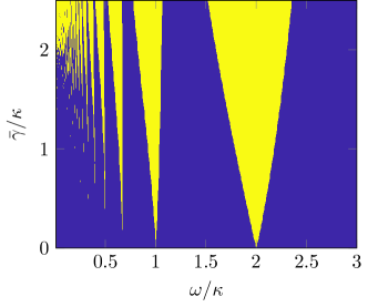
Figure 1: $\mathcal{PT}\,$phase diagram of the passive coupler with modulated loss $\gamma(z)$ from Eq. (11). For Lyapunov exponents that split from the mean loss values, the system is in the $\mathcal{PT}\,$-broken phase (yellow).

As an example, we consider a single photon propagating through the two-mode waveguide system. In Fig. 1, the resulting $\mathcal{PT}\,$phase diagram is shown as a function of the modulation frequency $\omega$ and the maximum loss $\bar{\gamma}$, normalized with respect to the coupling constant $\kappa$ between the waveguides. The $\mathcal{PT}\,$-broken phase is shaded in yellow. The diagram shows a clear reduction of the $\mathcal{PT}\,$-breaking threshold at the resonance frequency $\omega=2\kappa$ of the lossless coupler, with additional regions of reduced thresholds for lower modulation frequencies. A similar behaviour was also observed in a different context LeeJoglekar , thus pointing at a universal behaviour. Preparing the passive system with a loss modulation frequency equal to the resonance frequency might therefore enable one to efficiently probe the transition between $\mathcal{PT}\,$-symmetric and broken phases.

Note that the $\mathcal{PT}\,$phase diagram as calculated in Liouville space is identical to the Hilbert space phase diagram calculated from an effective non-Hermitian Hamiltonian of an active two-mode $\mathcal{PT}\,$system. If this were not true, the passive system would not be viable to simulate the active system. That this is indeed the case can be deduced from the decomposition of the algebra and the subsequent product form of the evolution superoperators. The superoperators $L_{i}^{-}R_{j}^{-}$ that are responsible for removing photons, as well as the sum of superoperators responsible for the mean loss, are clearly separated from the $\mathfrak{sl}(2,\mathbb{C})$ algebras that describe the underyling active $\mathcal{PT}\,$coupler. When postselecting on the outcome where no photon is lost in transmission, the contributions from $L_{i}^{-}R_{j}^{-}$ can be dismissed, and the only remaining part is an evolution governed by the effective non-Hermitian Hamiltonian of the active $\mathcal{PT}\,$system plus an overall mean loss. However, this mean loss is now greatly reduced at the resonance frequency $\omega=2\kappa$ compared to the unmodulated case where the threshold is $\bar{\gamma}=2\kappa$. Additionally, because we already solved for the monodromy, we are also able to calculate the full quantum evolution over all subspaces without the need for postselection.

We highlight one example of how the $\mathcal{PT}\,$phase transition manifests itself by calculating the occupation $P(n,h,z)$ of states $|n-h,h\rangle$

$$P(n,h;z)=\langle n-h,h|\hat{\rho}(z)|n-h,h\rangle,$$ (12)

over different subspaces with photon numbers $n$. Starting with the input state $|\psi\rangle=(|0,3\rangle+|3,0\rangle)/\sqrt{2}$, we show in Fig. 2 the evolution of all photon-number subspaces using a coupling constant $\kappa=1$. In the left figure, the system has a loss amplitude $\bar{\gamma}=0.25\kappa$ and a modulation frequency $\omega=1.5\kappa$ associated with the $\mathcal{PT}\,$-symmetric phase (see Fig. 1), whereas in the right figure, the modulation frequency is set to $\omega=2\kappa$ associated with the $\mathcal{PT}\,$-broken phase.

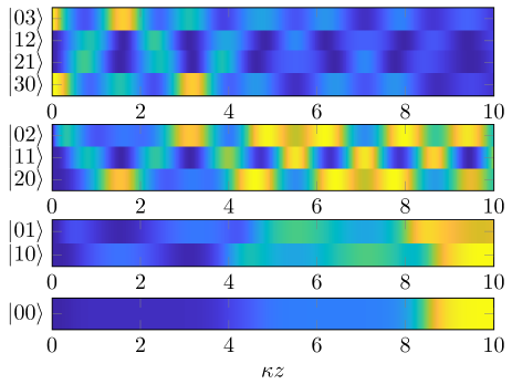
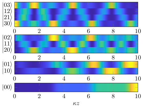
Figure 2: Occupations $P(n,h;z)$ for states $|n-h,h\rangle$ with input state $|\psi\rangle=(|0,3\rangle+|3,0\rangle)/\sqrt{2}$ over all subspaces with photon numbers $n\in\{0,1,2,3\}$. (Left) $\mathcal{PT}\,$-symmetric phase ($\bar{\gamma}=0.25\kappa$, $\omega=1.5\kappa$). (Right) $\mathcal{PT}\,$-broken phase ($\bar{\gamma}=0.25\kappa$, $\omega=2\kappa$).

This is reflected in the general behaviour of the occupations $P(n,h,z)$. In the left panel of Fig. 2, there are two oscillating strands that are equally damped by an overall loss. In contrast, the panel on the right shows one strongly damped strand and one with significantly lower loss. This behaviour is repeated across all subspaces except the continuously filled vacuum subspace (lowest subpanels). Note also that all subspaces with fewer than 3 photons are only transiently occupied.

The qualitative difference of the two evolutions is a clear sign of a $\mathcal{PT}\,$symmetry breaking where the system transitions from a coherent evolution (plus overall loss in the passive scheme) to an evolution that splits into exponentially decaying and growing modes. The physical explanation for this behaviour is that the damping of the $z$-dependent Floquet modes depend on whether or not they are concentrated in states $|n-h,h\rangle$ with more photons in the lossy waveguide when $\gamma(z)$ is large. This is the Floquet analogue of the usual signature of broken $\mathcal{PT}\,$symmetry of one mode being amplified and the other one being suppressed.

Recall that this $\mathcal{PT}\,$-symmetry breaking is only initiated by a change of the modulation frequency $\omega$, and that the loss amplitude $\bar{\gamma}$ is held at a low and constant value. In the static case, one instead has to change the loss rate to higher values that lead to significantly reduced visibilities in the measurements. The passive Floquet $\mathcal{PT}\,$coupler is therefore a possible way to probe the $\mathcal{PT}\,$phase transition without the obstacle of the overall loss. This is especially interesting as the required loss rate might even be further reduced as seen from the phase diagram Fig. 1. However, as the range of frequencies, for which $\mathcal{PT}\,$-symmetry is broken, becomes progressively narrower with decreasing values of $\bar{\gamma}$, an experimental implementation becomes more challenging.

Finally, we present a proposal on how to implement such a lossy coupler using auxiliary waveguides. The general principle is depicted in the lower part of Fig. 3. The top pair of waveguides, together with their mutual coupling $\kappa$, constitute the system under investigation. The lower waveguide of the pair is additionally coupled to a homogeneous array of $N$ auxiliary waveguides (the reservoir) with the coupling $\kappa_{l}$, while the coupling inside the reservoir is denoted by $\kappa_{b}$. In order to concentrate on the loss implementation, we briefly consider only one active system waveguide ($\kappa=0$). In the weak-coupling regime where $\kappa_{l}\ll\kappa_{b}$, the population in the system waveguide approximately shows an exponential decay with rate

$$\gamma=\frac{2\kappa^{2}_{l}}{\sqrt{\kappa_{b}^{2}-\kappa^{2}_{l}}}$$ (13)

after some short initial parabolic decay Longhi06 . For $N\to\infty$, the lost population does not return to the system waveguide, and hence constitutes a Markovian loss. For finite $N$, the exponential decay is only a good approximation up to some recurrence time due to reflections at the end of the array, which scales linearly with the array size. However, a sufficient number of auxiliary waveguides is easily obtainable in experiments Dreisow08 .

A modulated loss can then be implemented by modulating the coupling $\kappa_{l}$ which, in the evanscent coupling of the intregated photonic waveguides has the general form $\kappa_{l}(z)=A\exp[-\alpha d(z)]$, where $d(z)$ is the distance between waveguides and $A$ and $\alpha$ are appropriate scaling factors. With a modulation function $d(z)\propto\frac{1}{2}(1-\cos{(\omega z)})$, Eq. (13) yields the loss rate in Eq. (11). Note that the modulation has to be sufficiently slow for the resulting decay to follow an exponential law, i.e. that it can be described by a rate that yields the correct form of the dissipator of the quantum master equation (1).

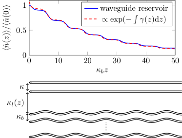
Figure 3: (Top) Decay of the mean photon number in the system waveguide by coupling to a modulated reservoir of waveguides (blue solid line) and comparison to analytical form of decay (red dashed line). (Bottom) Sketch of the modulated reservoir coupled to system waveguides.

In order to check the validity of our assumptions, we compared the numerical evaluation of the $N+1$ waveguide model with the behaviour of a lossy waveguide with a modulated decay rate ($\propto\exp{(-\int\gamma(z)\mathrm{d}z)}$ with $\gamma(z)$ given by Eq. (11). The result is shown in the upper panel in Fig. 3 for $\bar{\gamma}=0.125\kappa_{b}$ and $\omega=\kappa_{b}$. Setting $\kappa=0.5\kappa_{b}$ this corresponds to the example of the $\mathcal{PT}\,$-broken phase with $\bar{\gamma}=0.25\kappa$ and $\omega=2\kappa$ (right panel in Fig. 2). Note that the initial parabolic decay in the analytical approximation (dashed line) was accounted for by appropriate normalization Longhi06 . The numerical result (solid line) for the $N+1$ waveguide system matches the exponential decay with modulated frequency [Eq. (13)] very well. After re-introducing the system coupling $\kappa>0$, the loss still follows the exponential decay very closely, thus enabling the simulation of the Floquet $\mathcal{PT}\,$coupler.

In conclusion, we presented a method to probe the $\mathcal{PT}\,$-breaking transition in a passive Floquet $\mathcal{PT}\,$coupler with a modulated loss rate $\gamma(z)$. The $\mathcal{PT}\,$phase diagram was calculated for a functional form of the loss rate suitable for the implementation using evanscently coupled photonic waveguides. We showed that a phase transition occurs at considerably lower loss rates compared to the static case, which provides a feasible route to study $\mathcal{PT}\,$-symmetry breaking in quantum optical systems, in which modulated losses can be tailored by reservoir engineering.

This work was supported by the Deutsche Forschungsgemeinschaft (DFG) through grant SCHE 612/6-1.

References

- (1) C. M. Bender and S. Boettcher, Real spectra in non-Hermitian Hamiltonians having symmetry, Phys. Rev. Lett. 80, 5243 (1998).
- (2) W. D. Heiss, The physics of exceptional points, J. Phys. A: Math. Theor. 45, 444016 (2012).
- (3) H. Hodaei et al., Enhanced sensitivity at higher-order exceptional points, Nature 548, 187 (2017).
- (4) Jörg Doppler et al., Dynamically encircling an exceptional point for asymmetric mode switching, Nature 537, 76 (2016).
- (5) C. Dembowski et al., Experimental Observation of the Topological Structure of Exceptional Points, Phys. Rev. Lett. 86, 787 (2001).
- (6) J. Schindler et al., Experimental study of active LRC circuits with PT symmetries, Phys. Rev. A 84, 040101(R) (2011).
- (7) C. E. Rüter et al., Observation of parity-time symmetry in optics, Nat. Phys. 6, 192 (2010).
- (8) W. Chen, Ş. K. Özdemir, G. Zhao, J. Wiersig, and L. Yang, Exceptional points enhance sensing in an optical microcavity, Nature 548, 192 (2017).
- (9) M.-A. Miri and A. Alù, Exceptional points in optics and photonics, Science 363, 42 (2019).
- (10) F. Klauck et al., Observation of PT-symmetric quantum interference, Nat. Photon. 13, 883 (2019).
- (11) M. Naghiloo, M. Abbasi, Y. N. Joglekar, and K. W. Murch, Quantum state tomography across the exceptional point in a single dissipative qubit, Nat. Phys. 15, 1232 (2019).
- (12) S. Scheel and A. Szameit, -symmetric photonic quantum systems with gain and loss do not exist, Eur. Phys. Lett. 122, 34001 (2018).
- (13) L. Teuber and S. Scheel, Solving the quantum master equation of coupled harmonic oscillators with Lie-algebra methods, Phys. Rev. A 101, 042124 (2020).
- (14) M. A. Quiroz-Juárez et al., Exceptional points of any order in a single, lossy waveguide beam splitter by photon-number-resolved detection, Photonics Res. 7, 862 (2019).
- (15) J. Wiersig, Review of exceptional point-based sensors, Photonics Res. 8, 1457 (2020).
- (16) H. Wang, Y.-H. Lai, Z. Yuan, M.-G. Suh, and K. Vahala, Petermann-factor sensitivity limit near an exceptional point in a Brillouin ring laser gyroscope, Nat. Commun. 11, 1610 (2020).
- (17) M. Holthaus, Floquet engineering with quasienergy bands of periodically driven optical lattices, J. Phys. B: At. Mol. Opt. Phys. 49, 013001 (2016).
- (18) T. E. Lee and Y. N. Joglekar, -symmetric Rabi model: Perturbation theory, Phys. Rev. A 93, 042103 (2015).
- (19) J. Gunderson, J. Muldoon, K. W. Murch, and Y. N. Joglekar, Floquet exceptional contours in Lindblad dynamics with time-periodic drive and dissipation, preprint: 2011.02054 [quant-ph]
- (20) J. Wei and E. Norman, Lie Algebraic Solution of Linear Differential Equations, J. Math. Phys. 4, 575 (1963).
- (21) T. Meany et al., Laser written circuits for quantum optics, Laser Photonics Rev. 9, 363 (2015).
- (22) F. Dreisow, A. Szameit, M. Heinrich, T. Pertsch, S. Nolte, A. Tünnermann, and S. Longhi, Decay control via discrete-continuum modulation in optical waveguides, Conference on Lasers and Electro-Optics/Quantum Electronics and Laser Science Conference and Photonic Applications Systems Technologies (2008).
- (23) M. Ban, Lie-algebra methods in quantum optics: The Liouville-space formalism, Phys. Rev. A 47, 5093 (1993).
- (24) R. Gilmore, Lie Groups, Physics, and Geometry: An Introduction for Physicists, Engineers and Chemists (Cambridge University Press, 2008).
- (25) F. Wolf and H. J. Korsch, Time-evolution operators for (coupled) time-dependent oscillators and Lie algebraic structure theory, Phys. Rev. A 37, 1934 (1988).
- (26) S. Longhi, Nonexponential Decay Via Tunneling in Tight-Binding Lattices and the Optical Zeno Effect, Phys. Rev. Lett. 97, 110402 (2006).
- (27) S. Longhi, Control of photon tunneling in optical waveguides, Opt. Lett. 32, 557 (2007).
- (28) F. Dreisow, A. Szameit, M. Heinrich, T. Pertsch, S. Nolte, A. Tünnermann, and S. Longhi, Decay Control via Discrete-to-Continuum Coupling Modulation in an Optical Waveguide System, Phys. Rev. Lett. 101, 143602 (2008).