1 Introduction
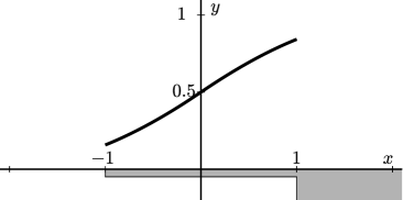
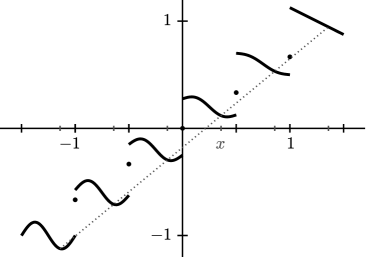
Imagine you are standing at a point x 𝑥 x [ − 1 , 1 ] 1 1 [-1,1] − 1 ≤ r ≤ 1 1 𝑟 1 -1\leq r\leq 1 r 𝑟 r | r | 𝑟 |r| x = − 1 𝑥 1 x=-1 x > 1 𝑥 1 x>1 x < − 1 𝑥 1 x<-1
Figure 1 : The probability y 𝑦 y x ∈ [ − 1 , 1 ] 𝑥 1 1 x\in[-1,1]
We shall see that the answer is
1 2 ( cos ( 1 / 2 ) 1 − sin ( 1 / 2 ) sin ( x / 2 ) + 1 − sgn ( x ) [ 1 − cos ( x / 2 ) ] ) . 1 2 1 2 1 1 2 𝑥 2 1 sgn 𝑥 delimited-[] 1 𝑥 2 \frac{1}{2}\left(\frac{\cos(1/2)}{1-\sin(1/2)}\sin(x/2)+1-\operatorname{sgn}(x)\Big{[}1-\cos(x/2)\Big{]}\right).
It is the solution to the mean value equation
u ( x ) = 1 2 ∫ x − 1 x + 1 u ( y ) d y , x ∈ [ − 1 , 1 ] , formulae-sequence 𝑢 𝑥 1 2 superscript subscript 𝑥 1 𝑥 1 𝑢 𝑦 differential-d 𝑦 𝑥 1 1 u(x)=\frac{1}{2}\int_{x-1}^{x+1}u(y)\mathrm{\,d}y,\qquad x\in[-1,1],
with boundary conditions
u ( x ) = { 0 , − 2 ≤ x < − 1 , 1 , 1 < x ≤ 2 . 𝑢 𝑥 cases 0 2 𝑥 1 1 1 𝑥 2 u(x)=\begin{cases}0,\qquad&-2\leq x<-1,\\
1,&1<x\leq 2.\end{cases}
The equation above is a special case of the nonlinear problem
u ( x ) 𝑢 𝑥 \displaystyle u(x) = N + 2 N + p ⨏ B ϵ ( x ) u ( y ) d y + p − 2 N + p sup | ξ | = 1 u ( x − ϵ ξ ) + u ( x + ϵ ξ ) 2 , absent 𝑁 2 𝑁 𝑝 subscript average-integral subscript 𝐵 italic-ϵ 𝑥 𝑢 𝑦 differential-d 𝑦 𝑝 2 𝑁 𝑝 subscript supremum 𝜉 1 𝑢 𝑥 italic-ϵ 𝜉 𝑢 𝑥 italic-ϵ 𝜉 2 \displaystyle=\tfrac{N+2}{N+p}\fint_{B_{\epsilon}(x)}u(y)\mathrm{\,d}y+\tfrac{p-2}{N+p}\sup_{|\xi|=1}\frac{u(x-\epsilon\xi)+u(x+\epsilon\xi)}{2}, x ∈ Ω ¯ , 𝑥 ¯ Ω \displaystyle x\in\overline{\Omega}, (1.1)
u ( x ) 𝑢 𝑥 \displaystyle u(x) = f ( x ) , absent 𝑓 𝑥 \displaystyle=f(x), x ∈ Γ ϵ , 𝑥 superscript Γ italic-ϵ \displaystyle x\in\Gamma^{\epsilon}, (1.2)
which is investigated in the paper [BLM20 ] .
Here, p ∈ [ 2 , ∞ ) 𝑝 2 p\in[2,\infty) ϵ > 0 italic-ϵ 0 \epsilon>0 Ω ⊆ ℝ N Ω superscript ℝ 𝑁 \Omega\subseteq\mathbb{R}^{N} Γ ϵ := { x ∉ Ω ¯ | dist ( x , Ω ) ≤ ϵ } assign superscript Γ italic-ϵ conditional-set 𝑥 ¯ Ω dist 𝑥 Ω italic-ϵ \Gamma^{\epsilon}:=\{x\notin\overline{\Omega}\;|\;\operatorname{dist}(x,\Omega)\leq\epsilon\} ϵ italic-ϵ \epsilon f : Γ ϵ ∪ ∂ Ω → ℝ : 𝑓 → superscript Γ italic-ϵ Ω ℝ f\colon\Gamma^{\epsilon}\cup\partial\Omega\to\mathbb{R} 1.1 p 𝑝 p
0 = 𝒟 p u := Δ u + ( p − 2 ) λ max ( D 2 u ) 0 subscript 𝒟 𝑝 𝑢 assign Δ 𝑢 𝑝 2 subscript 𝜆 superscript 𝐷 2 𝑢 0=\mathcal{D}_{p}u:=\Delta u+(p-2)\lambda_{\max}(D^{2}u)
in the sense that, if we denote the mean value operator by ℳ p ϵ superscript subscript ℳ 𝑝 italic-ϵ \mathcal{M}_{p}^{\epsilon}
ℳ p ϵ ϕ ( x ) − ϕ ( x ) = ϵ 2 2 ( N + p ) 𝒟 p ϕ ( x ) + o ( ϵ 2 ) superscript subscript ℳ 𝑝 italic-ϵ italic-ϕ 𝑥 italic-ϕ 𝑥 superscript italic-ϵ 2 2 𝑁 𝑝 subscript 𝒟 𝑝 italic-ϕ 𝑥 𝑜 superscript italic-ϵ 2 \mathcal{M}_{p}^{\epsilon}\phi(x)-\phi(x)=\frac{\epsilon^{2}}{2(N+p)}\mathcal{D}_{p}\phi(x)+o(\epsilon^{2})
as ϵ → 0 → italic-ϵ 0 \epsilon\to 0 C 2 superscript 𝐶 2 C^{2} ϕ italic-ϕ \phi 𝒟 p subscript 𝒟 𝑝 \mathcal{D}_{p} [Bru20 ] in order to explain a superposition principle in the p 𝑝 p
By Lemma 2.2 in [BLM20 ] we know that there is a unique solution to (1.1 1.2
u ( x ) 𝑢 𝑥 \displaystyle u(x) = 3 p + 1 ⋅ 1 2 ϵ ∫ x − ϵ x + ϵ u ( y ) d y + p − 2 p + 1 ⋅ 1 2 ( u ( x − ϵ ) + u ( x + ϵ ) ) , x ∈ [ a , b ] , formulae-sequence absent ⋅ 3 𝑝 1 1 2 italic-ϵ superscript subscript 𝑥 italic-ϵ 𝑥 italic-ϵ 𝑢 𝑦 differential-d 𝑦 ⋅ 𝑝 2 𝑝 1 1 2 𝑢 𝑥 italic-ϵ 𝑢 𝑥 italic-ϵ 𝑥 𝑎 𝑏 \displaystyle=\tfrac{3}{p+1}\cdot\tfrac{1}{2\epsilon}\int_{x-\epsilon}^{x+\epsilon}u(y)\mathrm{\,d}y+\tfrac{p-2}{p+1}\cdot\tfrac{1}{2}\Big{(}u(x-\epsilon)+u(x+\epsilon)\Big{)},\qquad x\in[a,b], (1.3)
u ( x ) 𝑢 𝑥 \displaystyle u(x) = f ( x ) , x ∈ [ a − ϵ , a ) ∪ ( b , b + ϵ ] . formulae-sequence absent 𝑓 𝑥 𝑥 𝑎 italic-ϵ 𝑎 𝑏 𝑏 italic-ϵ \displaystyle=f(x),\hskip 195.0ptx\in[a-\epsilon,a)\cup(b,b+\epsilon].
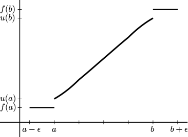
That is, when N = 1 𝑁 1 N=1 Ω = ( a , b ) Ω 𝑎 𝑏 \Omega=(a,b) ℝ ℝ \mathbb{R} ϵ = ( b − a ) / n italic-ϵ 𝑏 𝑎 𝑛 \epsilon=(b-a)/n n = 2 m 𝑛 2 𝑚 n=2m f 𝑓 f [BLM20 ] states that the solutions of (1.1 1.2 ϵ → 0 → italic-ϵ 0 \epsilon\to 0 u ′′ ( x ) = 0 superscript 𝑢 ′′ 𝑥 0 u^{\prime\prime}(x)=0 f ( a ) 𝑓 𝑎 f(a) f ( b ) 𝑓 𝑏 f(b) p = 2 𝑝 2 p=2 p > 2 𝑝 2 p>2
u ( x ) 𝑢 𝑥 \displaystyle u(x) = 1 2 ( u ( x − ϵ ) + u ( x + ϵ ) ) , absent 1 2 𝑢 𝑥 italic-ϵ 𝑢 𝑥 italic-ϵ \displaystyle=\frac{1}{2}\Big{(}u(x-\epsilon)+u(x+\epsilon)\Big{)}, x 𝑥 \displaystyle x ∈ [ a , b ] , absent 𝑎 𝑏 \displaystyle\in[a,b], (1.4)
u ( x ) 𝑢 𝑥 \displaystyle u(x) = f ( x ) , absent 𝑓 𝑥 \displaystyle=f(x), x 𝑥 \displaystyle x ∈ [ a − ϵ , a ) ∪ ( b , b + ϵ ] absent 𝑎 italic-ϵ 𝑎 𝑏 𝑏 italic-ϵ \displaystyle\in[a-\epsilon,a)\cup(b,b+\epsilon]
which is obtained by sending p → ∞ → 𝑝 p\to\infty
The stochastic interpretation of the Dirichlet problem (1.3 x 0 ∈ [ a , b ] subscript 𝑥 0 𝑎 𝑏 x_{0}\in[a,b] ϵ italic-ϵ \epsilon
{ with probability 3 p + 1 , the point x k + 1 ∈ [ x k − ϵ , x k + ϵ ] is picked at random. with probability 1 2 ⋅ p − 2 p + 1 , we set x k + 1 = x k − ϵ . with probability 1 2 ⋅ p − 2 p + 1 , we set x k + 1 = x k + ϵ . cases with probability 3 p + 1 , the point x k + 1 ∈ [ x k − ϵ , x k + ϵ ] is picked at random. otherwise with probability 1 2 ⋅ p − 2 p + 1 , we set x k + 1 = x k − ϵ . otherwise with probability 1 2 ⋅ p − 2 p + 1 , we set x k + 1 = x k + ϵ . otherwise \begin{cases}\text{with probability $\frac{3}{p+1}$, the point $x_{k+1}\in[x_{k}-\epsilon,x_{k}+\epsilon]$ is picked at random.}\\
\text{with probability $\frac{1}{2}\cdot\frac{p-2}{p+1}$, we set $x_{k+1}=x_{k}-\epsilon$.}\\
\text{with probability $\frac{1}{2}\cdot\frac{p-2}{p+1}$, we set $x_{k+1}=x_{k}+\epsilon$.}\end{cases} (1.5)
You stop the walk once you have left [ a , b ] 𝑎 𝑏 [a,b] k = τ 𝑘 𝜏 k=\tau u ( x 0 ) 𝑢 subscript 𝑥 0 u(x_{0}) expected value of the random variable f ( x τ ) 𝑓 subscript 𝑥 𝜏 f(x_{\tau}) f = 0 𝑓 0 f=0 [ a − ϵ , a ] 𝑎 italic-ϵ 𝑎 [a-\epsilon,a] f = 1 𝑓 1 f=1 [ b , b + ϵ ] 𝑏 𝑏 italic-ϵ [b,b+\epsilon] u ( x ) 𝑢 𝑥 u(x) probability of exiting at the right when starting the walk from x 𝑥 x
Note that the sup supremum \sup 1.3 control over the stochastic process in one dimension and the equation remains linear for p > 2 𝑝 2 p>2
2 The nonlocal Laplace equation with uniform distribution
With N = 1 𝑁 1 N=1 p = 2 𝑝 2 p=2
{ u ( x ) = 1 2 ϵ ∫ x − ϵ x + ϵ u ( y ) d y , for x ∈ [ a , b ] , u ( x ) = f ( x ) , for x ∈ [ a − ϵ , a ) ∪ ( b , b + ϵ ] . cases 𝑢 𝑥 1 2 italic-ϵ superscript subscript 𝑥 italic-ϵ 𝑥 italic-ϵ 𝑢 𝑦 differential-d 𝑦 for x ∈ [ a , b ] 𝑢 𝑥 𝑓 𝑥 for x ∈ [ a − ϵ , a ) ∪ ( b , b + ϵ ] \begin{cases}u(x)=\displaystyle\frac{1}{2\epsilon}\int_{x-\epsilon}^{x+\epsilon}u(y)\mathrm{\,d}y,\qquad&\text{for $x\in[a,b]$},\\
u(x)=f(x),&\text{for $x\in[a-\epsilon,a)\cup(b,b+\epsilon]$}.\end{cases} (2.1)
If f 𝑓 f u 𝑢 u piecewise trigonometric function . Specifically, on each of the n 𝑛 n [ a + ( k − 1 ) ϵ , a + k ϵ ] 𝑎 𝑘 1 italic-ϵ 𝑎 𝑘 italic-ϵ [a+(k-1)\epsilon,a+k\epsilon] k = 1 , … , n 𝑘 1 … 𝑛
k=1,\dots,n ϵ italic-ϵ \epsilon u 𝑢 u
u ( x ) = a k + ∑ j = 1 m b k , j sin ( λ j ϵ x ) + c k , j cos ( λ j ϵ x ) 𝑢 𝑥 subscript 𝑎 𝑘 superscript subscript 𝑗 1 𝑚 subscript 𝑏 𝑘 𝑗
subscript 𝜆 𝑗 italic-ϵ 𝑥 subscript 𝑐 𝑘 𝑗
subscript 𝜆 𝑗 italic-ϵ 𝑥 u(x)=a_{k}+\sum_{j=1}^{m}b_{k,j}\sin\left(\frac{\lambda_{j}}{\epsilon}x\right)+c_{k,j}\cos\left(\frac{\lambda_{j}}{\epsilon}x\right) (2.2)
for computable coefficients a k , b k , j , c k , j subscript 𝑎 𝑘 subscript 𝑏 𝑘 𝑗
subscript 𝑐 𝑘 𝑗
a_{k},b_{k,j},c_{k,j}
λ j = cos ( j π n + 1 ) . subscript 𝜆 𝑗 𝑗 𝜋 𝑛 1 \lambda_{j}=\cos\left(\frac{j\pi}{n+1}\right).
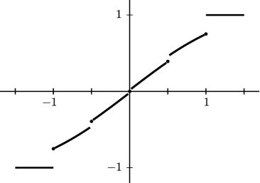
When f 𝑓 f 2.5 [ a , b ] = [ − 1 , 1 ] 𝑎 𝑏 1 1 [a,b]=[-1,1]
Figure 2 : The solution of (2.1 n = 4 𝑛 4 n=4 Figure 3 : Convergence of the boundary values.
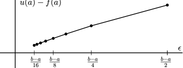
Although the solution has oscillations for all ϵ = ( b − a ) / n italic-ϵ 𝑏 𝑎 𝑛 \epsilon=(b-a)/n n ≥ 4 𝑛 4 n\geq 4 u ( a ) → f ( a ) → 𝑢 𝑎 𝑓 𝑎 u(a)\to f(a) u ( b ) → f ( b ) → 𝑢 𝑏 𝑓 𝑏 u(b)\to f(b) ϵ italic-ϵ \epsilon 3 [BLM20 ] ) ensures that the convergence is linear, since the solution has to lie between the two lines passing through the points ( a − ϵ , f ( a ) ) , ( b , f ( b ) ) 𝑎 italic-ϵ 𝑓 𝑎 𝑏 𝑓 𝑏
(a-\epsilon,f(a)),(b,f(b)) ( a , f ( a ) ) , ( b + ϵ , f ( b ) ) 𝑎 𝑓 𝑎 𝑏 italic-ϵ 𝑓 𝑏
(a,f(a)),(b+\epsilon,f(b)) N ≥ 2 𝑁 2 N\geq 2
2.1 The functional differential equation
One may easily show that the solution u 𝑢 u 2.1 C / ( 2 ϵ ) 𝐶 2 italic-ϵ C/(2\epsilon) [ a , b ] 𝑎 𝑏 [a,b] C = max f − min f 𝐶 𝑓 𝑓 C=\max f-\min f u 𝑢 u ( a , b ) ∖ { a + ϵ , b − ϵ } 𝑎 𝑏 𝑎 italic-ϵ 𝑏 italic-ϵ (a,b)\setminus\{a+\epsilon,b-\epsilon\}
u ′ ( x ) = 1 2 ϵ ( u ( x + ϵ ) − u ( x − ϵ ) ) . superscript 𝑢 ′ 𝑥 1 2 italic-ϵ 𝑢 𝑥 italic-ϵ 𝑢 𝑥 italic-ϵ u^{\prime}(x)=\frac{1}{2\epsilon}\Big{(}u(x+\epsilon)-u(x-\epsilon)\Big{)}. (2.3)
u 𝑢 u a + ϵ 𝑎 italic-ϵ a+\epsilon b − ϵ 𝑏 italic-ϵ b-\epsilon u 𝑢 u a 𝑎 a b 𝑏 b 2 u 𝑢 u 2.3 u 𝑢 u [ a , b ] 𝑎 𝑏 [a,b]
2.2 Constant boundary values
Let u 𝑢 u
{ u ( x ) = 1 2 ϵ ∫ x − ϵ x + ϵ u ( y ) d y , for x ∈ [ a , b ] , u ( x ) = c l , for x ∈ [ a − ϵ , a ) , u ( x ) = c r , for x ∈ ( b , b + ϵ ] . cases 𝑢 𝑥 1 2 italic-ϵ superscript subscript 𝑥 italic-ϵ 𝑥 italic-ϵ 𝑢 𝑦 differential-d 𝑦 for x ∈ [ a , b ] 𝑢 𝑥 subscript 𝑐 𝑙 for x ∈ [ a − ϵ , a ) 𝑢 𝑥 subscript 𝑐 𝑟 for x ∈ ( b , b + ϵ ] \begin{cases}u(x)=\displaystyle\frac{1}{2\epsilon}\int_{x-\epsilon}^{x+\epsilon}u(y)\mathrm{\,d}y,\qquad&\text{for $x\in[a,b]$},\\
u(x)=c_{l},&\text{for $x\in[a-\epsilon,a)$},\\
u(x)=c_{r},&\text{for $x\in(b,b+\epsilon]$}.\end{cases} (2.4)
where a < b 𝑎 𝑏 a<b ϵ = ( b − a ) / n italic-ϵ 𝑏 𝑎 𝑛 \epsilon=(b-a)/n n = 2 m 𝑛 2 𝑚 n=2m c l ≠ c r subscript 𝑐 𝑙 subscript 𝑐 𝑟 c_{l}\neq c_{r} c l = c r subscript 𝑐 𝑙 subscript 𝑐 𝑟 c_{l}=c_{r}
To exploit the symmetry in the problem, we assume that u 𝑢 u [ a , b ] = [ − 1 , 1 ] 𝑎 𝑏 1 1 [a,b]=[-1,1] c l = − 1 subscript 𝑐 𝑙 1 c_{l}=-1 c r = 1 subscript 𝑐 𝑟 1 c_{r}=1
Divide the domain into n 𝑛 n ϵ italic-ϵ \epsilon k = 1 , … , n 𝑘 1 … 𝑛
k=1,\dots,n v k : [ 0 , 1 ] → ℝ : subscript 𝑣 𝑘 → 0 1 ℝ v_{k}\colon[0,1]\to\mathbb{R}
v k ( t ) subscript 𝑣 𝑘 𝑡 \displaystyle v_{k}(t) := 2 c r − c l ( u ( ϵ t + a + ( k − 1 ) ϵ ) − c l + c r 2 ) assign absent 2 subscript 𝑐 𝑟 subscript 𝑐 𝑙 𝑢 italic-ϵ 𝑡 𝑎 𝑘 1 italic-ϵ subscript 𝑐 𝑙 subscript 𝑐 𝑟 2 \displaystyle:=\frac{2}{c_{r}-c_{l}}\left(u\big{(}\epsilon t+a+(k-1)\epsilon\big{)}-\frac{c_{l}+c_{r}}{2}\right) (2.5)
= u ( ϵ t − 1 + ( k − 1 ) ϵ ) . absent 𝑢 italic-ϵ 𝑡 1 𝑘 1 italic-ϵ \displaystyle=u\big{(}\epsilon t-1+(k-1)\epsilon\big{)}.
Now, each v k subscript 𝑣 𝑘 v_{k} ( 0 , 1 ) 0 1 (0,1) k = 1 𝑘 1 k=1 2.3
v 1 ′ ( t ) superscript subscript 𝑣 1 ′ 𝑡 \displaystyle v_{1}^{\prime}(t) = ϵ u ′ ( ϵ t − 1 ) absent italic-ϵ superscript 𝑢 ′ italic-ϵ 𝑡 1 \displaystyle=\epsilon u^{\prime}(\epsilon t-1)
= ϵ 1 2 ϵ ( u ( ϵ t − 1 + ϵ ) − u ( ϵ t − 1 − ϵ ) ) absent italic-ϵ 1 2 italic-ϵ 𝑢 italic-ϵ 𝑡 1 italic-ϵ 𝑢 italic-ϵ 𝑡 1 italic-ϵ \displaystyle=\epsilon\frac{1}{2\epsilon}\Big{(}u(\epsilon t-1+\epsilon)-u(\epsilon t-1-\epsilon)\Big{)}
= 1 2 ( u ( ϵ t − 1 + ϵ ) − c l ) absent 1 2 𝑢 italic-ϵ 𝑡 1 italic-ϵ subscript 𝑐 𝑙 \displaystyle=\frac{1}{2}\Big{(}u(\epsilon t-1+\epsilon)-c_{l}\Big{)}
= 1 2 ( v 2 ( t ) + 1 ) . absent 1 2 subscript 𝑣 2 𝑡 1 \displaystyle=\frac{1}{2}\Big{(}v_{2}(t)+1\Big{)}.
Similarly, v n ′ ( t ) = 1 2 ( 1 − v n − 1 ( t ) ) superscript subscript 𝑣 𝑛 ′ 𝑡 1 2 1 subscript 𝑣 𝑛 1 𝑡 v_{n}^{\prime}(t)=\frac{1}{2}\Big{(}1-v_{n-1}(t)\Big{)} k = 2 , … , n − 1 𝑘 2 … 𝑛 1
k=2,\dots,n-1
v k ′ ( t ) = 1 2 ( v k + 1 ( t ) − v k − 1 ( t ) ) . superscript subscript 𝑣 𝑘 ′ 𝑡 1 2 subscript 𝑣 𝑘 1 𝑡 subscript 𝑣 𝑘 1 𝑡 v_{k}^{\prime}(t)=\frac{1}{2}\Big{(}v_{k+1}(t)-v_{k-1}(t)\Big{)}.
This defines a non-homogeneous linear system of ODEs,
[ v 1 ′ v 2 ′ v 3 ′ ⋮ v n − 1 ′ v n ′ ] = 1 2 [ 0 1 0 0 ⋯ 0 − 1 0 1 0 ⋯ 0 0 − 1 0 1 ⋯ 0 ⋮ 0 ⋯ 0 − 1 0 1 0 ⋯ 0 0 − 1 0 ] [ v 1 v 2 v 3 ⋮ v n − 1 v n ] + 1 2 [ 1 0 0 ⋮ 0 1 ] , matrix subscript superscript 𝑣 ′ 1 superscript subscript 𝑣 2 ′ superscript subscript 𝑣 3 ′ ⋮ superscript subscript 𝑣 𝑛 1 ′ superscript subscript 𝑣 𝑛 ′ 1 2 matrix 0 1 0 0 ⋯ 0 1 0 1 0 ⋯ 0 0 1 0 1 ⋯ 0 missing-subexpression missing-subexpression ⋮ missing-subexpression missing-subexpression missing-subexpression 0 ⋯ 0 1 0 1 0 ⋯ 0 0 1 0 matrix subscript 𝑣 1 subscript 𝑣 2 subscript 𝑣 3 ⋮ subscript 𝑣 𝑛 1 subscript 𝑣 𝑛 1 2 matrix 1 0 0 ⋮ 0 1 \begin{bmatrix}v^{\prime}_{1}\\
v_{2}^{\prime}\\
v_{3}^{\prime}\\
\vdots\\
v_{n-1}^{\prime}\\
v_{n}^{\prime}\end{bmatrix}=\frac{1}{2}\begin{bmatrix}0&1&0&0&\cdots&0\\
-1&0&1&0&\cdots&0\\
0&-1&0&1&\cdots&0\\
&&\vdots&&&\\
0&\cdots&0&-1&0&1\\
0&\cdots&0&0&-1&0\end{bmatrix}\begin{bmatrix}v_{1}\\
v_{2}\\
v_{3}\\
\vdots\\
v_{n-1}\\
v_{n}\end{bmatrix}+\frac{1}{2}\begin{bmatrix}1\\
0\\
0\\
\vdots\\
0\\
1\end{bmatrix},
or
𝐯 ′ ( t ) = A 𝐯 ( t ) + 𝐜 superscript 𝐯 ′ 𝑡 𝐴 𝐯 𝑡 𝐜 \mathbf{v}^{\prime}(t)=A\mathbf{v}(t)+\mathbf{c} (2.6)
in vector notation.
The general solution is 𝐯 ( t ) = e t A ( 𝐯 0 + A − 1 𝐜 ) − A − 1 𝐜 𝐯 𝑡 superscript 𝑒 𝑡 𝐴 subscript 𝐯 0 superscript 𝐴 1 𝐜 superscript 𝐴 1 𝐜 \mathbf{v}(t)=e^{tA}(\mathbf{v}_{0}+A^{-1}\mathbf{c})-A^{-1}\mathbf{c}
e A := ∑ k = 0 ∞ 1 k ! A k assign superscript 𝑒 𝐴 superscript subscript 𝑘 0 1 𝑘 superscript 𝐴 𝑘 e^{A}:=\sum_{k=0}^{\infty}\frac{1}{k!}A^{k}
is the matrix exponential.
Defining
𝐞 ~ := ∑ k = 1 n ( − 1 ) k 𝐞 k , assign ~ 𝐞 superscript subscript 𝑘 1 𝑛 superscript 1 𝑘 subscript 𝐞 𝑘 \tilde{\mathbf{e}}:=\sum_{k=1}^{n}(-1)^{k}\mathbf{e}_{k},
we note that
A 𝐞 ~ = 1 2 [ 0 1 0 0 ⋯ 0 − 1 0 1 0 ⋯ 0 0 − 1 0 1 ⋯ 0 ⋮ ⋯ 1 0 ⋯ 0 − 1 0 ] [ − 1 1 − 1 ⋮ 1 ] = 1 2 [ 1 0 ⋮ 0 1 ] = 𝐜 𝐴 ~ 𝐞 1 2 matrix 0 1 0 0 ⋯ 0 1 0 1 0 ⋯ 0 0 1 0 1 ⋯ 0 missing-subexpression ⋮ missing-subexpression missing-subexpression ⋯ 1 0 ⋯ missing-subexpression 0 1 0 matrix 1 1 1 ⋮ 1 1 2 matrix 1 0 ⋮ 0 1 𝐜 A\tilde{\mathbf{e}}=\frac{1}{2}\begin{bmatrix}0&1&0&0&\cdots&0\\
-1&0&1&0&\cdots&0\\
0&-1&0&1&\cdots&0\\
&\vdots&&&\cdots&1\\
0&\cdots&&0&-1&0\end{bmatrix}\begin{bmatrix}-1\\
1\\
-1\\
\vdots\\
1\end{bmatrix}=\frac{1}{2}\begin{bmatrix}1\\
0\\
\vdots\\
0\\
1\end{bmatrix}=\mathbf{c}
and thus
𝐯 ( t ) = e t A ( 𝐯 0 + 𝐞 ~ ) − 𝐞 ~ . 𝐯 𝑡 superscript 𝑒 𝑡 𝐴 subscript 𝐯 0 ~ 𝐞 ~ 𝐞 \mathbf{v}(t)=e^{tA}(\mathbf{v}_{0}+\tilde{\mathbf{e}})-\tilde{\mathbf{e}}. (2.7)
The initial value 𝐯 0 = 𝐯 ( 0 ) subscript 𝐯 0 𝐯 0 \mathbf{v}_{0}=\mathbf{v}(0) u 𝑢 u − 1 + ( k − 1 ) ϵ 1 𝑘 1 italic-ϵ -1+(k-1)\epsilon n − 1 𝑛 1 n-1 v k ( 0 ) = v k − 1 ( 1 ) subscript 𝑣 𝑘 0 subscript 𝑣 𝑘 1 1 v_{k}(0)=v_{k-1}(1) k = 2 , … , n 𝑘 2 … 𝑛
k=2,\dots,n n 𝑛 n u 𝑢 u u ( − 1 ) = − u ( 1 ) 𝑢 1 𝑢 1 u(-1)=-u(1) v 1 ( 0 ) = − v n ( 1 ) subscript 𝑣 1 0 subscript 𝑣 𝑛 1 v_{1}(0)=-v_{n}(1)
𝐯 ( 0 ) = B 𝐯 ( 1 ) 𝐯 0 𝐵 𝐯 1 \mathbf{v}(0)=B\mathbf{v}(1) (2.8)
where B 𝐵 B
B := [ 0 0 0 ⋯ 0 − 1 1 0 0 ⋯ 0 0 0 1 0 ⋯ 0 0 ⋱ 0 ⋯ 0 1 0 ] = [ 𝟎 ⊤ − 1 I n − 1 𝟎 ] . assign 𝐵 matrix 0 0 0 ⋯ 0 1 1 0 0 ⋯ 0 0 0 1 0 ⋯ 0 0 missing-subexpression missing-subexpression ⋱ missing-subexpression missing-subexpression missing-subexpression 0 ⋯ missing-subexpression 0 1 0 matrix superscript 0 top 1 subscript 𝐼 𝑛 1 0 B:=\begin{bmatrix}0&0&0&\cdots&0&-1\\
1&0&0&\cdots&0&0\\
0&1&0&\cdots&0&0\\
&&\ddots&&&\\
0&\cdots&&0&1&0\end{bmatrix}=\begin{bmatrix}\bf 0^{\top}&-1\\
I_{n-1}&\bf 0\end{bmatrix}.
Inserting (2.7 2.8 t = 1 𝑡 1 t=1 u 𝑢 u [ − 1 , 1 ] 1 1 [-1,1] 𝐯 0 subscript 𝐯 0 \mathbf{v}_{0}
( I − B e A ) 𝐯 0 = B ( e A − I ) 𝐞 ~ , 𝐼 𝐵 superscript 𝑒 𝐴 subscript 𝐯 0 𝐵 superscript 𝑒 𝐴 𝐼 ~ 𝐞 (I-Be^{A})\mathbf{v}_{0}=B(e^{A}-I)\tilde{\mathbf{e}},
and the unique solution of (2.6 2.8
𝐯 ( t ) = e t A ( I − B e A ) − 1 ( I − B ) 𝐞 ~ − 𝐞 ~ , 0 ≤ t ≤ 1 . formulae-sequence 𝐯 𝑡 superscript 𝑒 𝑡 𝐴 superscript 𝐼 𝐵 superscript 𝑒 𝐴 1 𝐼 𝐵 ~ 𝐞 ~ 𝐞 0 𝑡 1 \mathbf{v}(t)=e^{tA}(I-Be^{A})^{-1}(I-B)\tilde{\mathbf{e}}-\tilde{\mathbf{e}},\qquad 0\leq t\leq 1.
The invertability of I − B e A 𝐼 𝐵 superscript 𝑒 𝐴 I-Be^{A} 𝐯 ( t ) 𝐯 𝑡 \mathbf{v}(t) n 𝑛 n
The solution u 𝑢 u 2.4 2.5
u ( x ) 𝑢 𝑥 \displaystyle u(x) = { c l , x ∈ [ a − ϵ , a ) , c r − c l 2 v k ( x − a ϵ + 1 − k ) + c r + c l 2 , x ∈ [ a + ( k − 1 ) ϵ , a + k ϵ ] , k = 1 , … , n , c r , x ∈ ( b , b + ϵ ] . absent cases subscript 𝑐 𝑙 𝑥 𝑎 italic-ϵ 𝑎 subscript 𝑐 𝑟 subscript 𝑐 𝑙 2 subscript 𝑣 𝑘 𝑥 𝑎 italic-ϵ 1 𝑘 subscript 𝑐 𝑟 subscript 𝑐 𝑙 2 formulae-sequence 𝑥 𝑎 𝑘 1 italic-ϵ 𝑎 𝑘 italic-ϵ 𝑘 1 … 𝑛
subscript 𝑐 𝑟 𝑥 𝑏 𝑏 italic-ϵ \displaystyle=\begin{cases}c_{l},\qquad&x\in[a-\epsilon,a),\\
\frac{c_{r}-c_{l}}{2}v_{k}\left(\frac{x-a}{\epsilon}+1-k\right)+\frac{c_{r}+c_{l}}{2},&x\in[a+(k-1)\epsilon,a+k\epsilon],\quad k=1,\dots,n,\\
c_{r},\qquad&x\in(b,b+\epsilon].\end{cases}
= { − 1 , x ∈ [ − 1 − ϵ , − 1 ) , v k ( x + 1 ϵ + 1 − k ) , x ∈ [ − 1 + ( k − 1 ) ϵ , − 1 + k ϵ ] , k = 1 , … , n , 1 , x ∈ ( 1 , 1 + ϵ ] . absent cases 1 𝑥 1 italic-ϵ 1 subscript 𝑣 𝑘 𝑥 1 italic-ϵ 1 𝑘 formulae-sequence 𝑥 1 𝑘 1 italic-ϵ 1 𝑘 italic-ϵ 𝑘 1 … 𝑛
1 𝑥 1 1 italic-ϵ \displaystyle=\begin{cases}-1,\qquad&x\in[-1-\epsilon,-1),\\
v_{k}\left(\frac{x+1}{\epsilon}+1-k\right),&x\in[-1+(k-1)\epsilon,-1+k\epsilon],\quad k=1,\dots,n,\\
1,\qquad&x\in(1,1+\epsilon].\end{cases}
2.3 Analysis
The coefficient matrix of the linear system is the skew-symmetric and tridiagonal n × n 𝑛 𝑛 n\times n
A := 1 2 [ 0 1 0 0 ⋯ 0 − 1 0 1 0 ⋯ 0 0 − 1 0 1 ⋯ 0 ⋮ ⋯ 1 0 ⋯ 0 − 1 0 ] assign 𝐴 1 2 matrix 0 1 0 0 ⋯ 0 1 0 1 0 ⋯ 0 0 1 0 1 ⋯ 0 missing-subexpression ⋮ missing-subexpression missing-subexpression ⋯ 1 0 ⋯ missing-subexpression 0 1 0 A:=\frac{1}{2}\begin{bmatrix}0&1&0&0&\cdots&0\\
-1&0&1&0&\cdots&0\\
0&-1&0&1&\cdots&0\\
&\vdots&&&\cdots&1\\
0&\cdots&&0&-1&0\end{bmatrix}
where n = 2 m 𝑛 2 𝑚 n=2m
In order to diagonalize A 𝐴 A ξ j ∈ ℂ n subscript 𝜉 𝑗 superscript ℂ 𝑛 \xi_{j}\in\mathbb{C}^{n}
𝐞 k ⊤ ξ j = c n i k + 2 j sin ( k j π n + 1 ) , c n := 2 n + 1 , i := − 1 . formulae-sequence superscript subscript 𝐞 𝑘 top subscript 𝜉 𝑗 subscript 𝑐 𝑛 superscript 𝑖 𝑘 2 𝑗 𝑘 𝑗 𝜋 𝑛 1 formulae-sequence assign subscript 𝑐 𝑛 2 𝑛 1 assign 𝑖 1 \mathbf{e}_{k}^{\top}\xi_{j}=c_{n}i^{k+2j}\sin\left(kj\frac{\pi}{n+1}\right),\qquad c_{n}:=\sqrt{\frac{2}{n+1}},\;i:=\sqrt{-1}.
They have unit length since
∑ k = 1 n sin 2 ( k j π n + 1 ) superscript subscript 𝑘 1 𝑛 superscript 2 𝑘 𝑗 𝜋 𝑛 1 \displaystyle\sum_{k=1}^{n}\sin^{2}\left(kj\frac{\pi}{n+1}\right) = n + 1 2 absent 𝑛 1 2 \displaystyle=\frac{n+1}{2}
by Lagrange’s identity. Using the rule
sin θ + sin ϕ = 2 cos ( θ − ϕ 2 ) sin ( θ + ϕ 2 ) , 𝜃 italic-ϕ 2 𝜃 italic-ϕ 2 𝜃 italic-ϕ 2 \sin\theta+\sin\phi=2\cos\left(\frac{\theta-\phi}{2}\right)\sin\left(\frac{\theta+\phi}{2}\right),
shows that
𝐞 k ⊤ A ξ j superscript subscript 𝐞 𝑘 top 𝐴 subscript 𝜉 𝑗 \displaystyle\mathbf{e}_{k}^{\top}A\xi_{j} = c n 2 ( i k + 2 j + 1 sin ( ( k + 1 ) j π n + 1 ) − i k − 1 + 2 j sin ( ( k − 1 ) j π n + 1 ) ) absent subscript 𝑐 𝑛 2 superscript 𝑖 𝑘 2 𝑗 1 𝑘 1 𝑗 𝜋 𝑛 1 superscript 𝑖 𝑘 1 2 𝑗 𝑘 1 𝑗 𝜋 𝑛 1 \displaystyle=\frac{c_{n}}{2}\left(i^{k+2j+1}\sin\left((k+1)j\frac{\pi}{n+1}\right)-i^{k-1+2j}\sin\left((k-1)j\frac{\pi}{n+1}\right)\right)
= i k + 1 + 2 j c n 2 ( sin ( ( k + 1 ) j π n + 1 ) + sin ( ( k − 1 ) j π n + 1 ) ) absent superscript 𝑖 𝑘 1 2 𝑗 subscript 𝑐 𝑛 2 𝑘 1 𝑗 𝜋 𝑛 1 𝑘 1 𝑗 𝜋 𝑛 1 \displaystyle=\frac{i^{k+1+2j}c_{n}}{2}\left(\sin\left((k+1)j\frac{\pi}{n+1}\right)+\sin\left((k-1)j\frac{\pi}{n+1}\right)\right)
= i k + 1 + 2 j c n cos ( j π n + 1 ) sin ( k j π n + 1 ) absent superscript 𝑖 𝑘 1 2 𝑗 subscript 𝑐 𝑛 𝑗 𝜋 𝑛 1 𝑘 𝑗 𝜋 𝑛 1 \displaystyle=i^{k+1+2j}c_{n}\cos\left(j\frac{\pi}{n+1}\right)\sin\left(kj\frac{\pi}{n+1}\right)
= i cos ( j π n + 1 ) 𝐞 k ⊤ ξ j . absent 𝑖 𝑗 𝜋 𝑛 1 superscript subscript 𝐞 𝑘 top subscript 𝜉 𝑗 \displaystyle=i\cos\left(j\frac{\pi}{n+1}\right)\mathbf{e}_{k}^{\top}\xi_{j}.
That is, ξ j subscript 𝜉 𝑗 \xi_{j} A 𝐴 A i cos ( j π n + 1 ) 𝑖 𝑗 𝜋 𝑛 1 i\cos\left(j\frac{\pi}{n+1}\right) j = 1 , … , m 𝑗 1 … 𝑚
j=1,\dots,m ξ n + 1 − j = ξ ¯ j subscript 𝜉 𝑛 1 𝑗 subscript ¯ 𝜉 𝑗 \xi_{n+1-j}=\overline{\xi}_{j} A 𝐴 A
U := [ ξ 1 , ξ ¯ 1 , … , ξ m , ξ ¯ m ] ∈ ℂ n × n , assign 𝑈 subscript 𝜉 1 subscript ¯ 𝜉 1 … subscript 𝜉 𝑚 subscript ¯ 𝜉 𝑚
superscript ℂ 𝑛 𝑛 U:=[\xi_{1},\overline{\xi}_{1},\dots,\xi_{m},\overline{\xi}_{m}]\in\mathbb{C}^{n\times n},
producing
Λ := U ¯ ⊤ A U = diag ( i λ 1 , − i λ 1 , … , i λ m , − i λ m ) assign Λ superscript ¯ 𝑈 top 𝐴 𝑈 diag 𝑖 subscript 𝜆 1 𝑖 subscript 𝜆 1 … 𝑖 subscript 𝜆 𝑚 𝑖 subscript 𝜆 𝑚 \Lambda:=\overline{U}^{\top}AU=\operatorname{diag}(i\lambda_{1},-i\lambda_{1},\dots,i\lambda_{m},-i\lambda_{m})
where
0 < λ j := cos ( j n + 1 π ) < 1 , j = 1 , … , m . formulae-sequence 0 subscript 𝜆 𝑗 assign 𝑗 𝑛 1 𝜋 1 𝑗 1 … 𝑚
0<\lambda_{j}:=\cos\left(\frac{j}{n+1}\pi\right)<1,\qquad j=1,\dots,m.
The real and imaginary parts of the eigenvectors ξ j = 𝐚 j + i 𝐛 j subscript 𝜉 𝑗 subscript 𝐚 𝑗 𝑖 subscript 𝐛 𝑗 \xi_{j}=\mathbf{a}_{j}+i\mathbf{b}_{j}
𝐚 j subscript 𝐚 𝑗 \displaystyle\mathbf{a}_{j} = c n ∑ k = 1 m ( − 1 ) k + j sin ( 2 k j π n + 1 ) 𝐞 2 k , absent subscript 𝑐 𝑛 superscript subscript 𝑘 1 𝑚 superscript 1 𝑘 𝑗 2 𝑘 𝑗 𝜋 𝑛 1 subscript 𝐞 2 𝑘 \displaystyle=c_{n}\sum_{k=1}^{m}(-1)^{k+j}\sin\left(2kj\frac{\pi}{n+1}\right)\mathbf{e}_{2k},
𝐛 j subscript 𝐛 𝑗 \displaystyle\mathbf{b}_{j} = c n ∑ k = 1 m ( − 1 ) k + j + 1 sin ( ( 2 k − 1 ) j π n + 1 ) 𝐞 2 k − 1 . absent subscript 𝑐 𝑛 superscript subscript 𝑘 1 𝑚 superscript 1 𝑘 𝑗 1 2 𝑘 1 𝑗 𝜋 𝑛 1 subscript 𝐞 2 𝑘 1 \displaystyle=c_{n}\sum_{k=1}^{m}(-1)^{k+j+1}\sin\left((2k-1)j\frac{\pi}{n+1}\right)\mathbf{e}_{2k-1}.
Here,
𝐚 j ⊤ 𝐛 k = 0 and 𝐚 j ⊤ 𝐚 k = 𝐛 j ⊤ 𝐛 k = δ j , k 2 formulae-sequence superscript subscript 𝐚 𝑗 top subscript 𝐛 𝑘 0 and
superscript subscript 𝐚 𝑗 top subscript 𝐚 𝑘 superscript subscript 𝐛 𝑗 top subscript 𝐛 𝑘 subscript 𝛿 𝑗 𝑘
2 \mathbf{a}_{j}^{\top}\mathbf{b}_{k}=0\qquad\text{and}\qquad\mathbf{a}_{j}^{\top}\mathbf{a}_{k}=\mathbf{b}_{j}^{\top}\mathbf{b}_{k}=\frac{\delta_{j,k}}{2}
since ξ j ⊤ ξ k = 0 superscript subscript 𝜉 𝑗 top subscript 𝜉 𝑘 0 \xi_{j}^{\top}\xi_{k}=0 ξ j ¯ ⊤ ξ k = δ j , k superscript ¯ subscript 𝜉 𝑗 top subscript 𝜉 𝑘 subscript 𝛿 𝑗 𝑘
\overline{\xi_{j}}^{\top}\xi_{k}=\delta_{j,k}
A j := − 2 Im ξ j ξ ¯ j ⊤ = 2 ( 𝐚 j 𝐛 j ⊤ − 𝐛 j 𝐚 j ⊤ ) , j = 1 , … , m , formulae-sequence assign subscript 𝐴 𝑗 2 Im subscript 𝜉 𝑗 superscript subscript ¯ 𝜉 𝑗 top 2 subscript 𝐚 𝑗 superscript subscript 𝐛 𝑗 top subscript 𝐛 𝑗 superscript subscript 𝐚 𝑗 top 𝑗 1 … 𝑚
A_{j}:=-2\operatorname{Im}\xi_{j}\overline{\xi}_{j}^{\top}=2(\mathbf{a}_{j}\mathbf{b}_{j}^{\top}-\mathbf{b}_{j}\mathbf{a}_{j}^{\top}),\qquad j=1,\dots,m,
then
A 𝐴 \displaystyle A = U Λ U ¯ ⊤ absent 𝑈 Λ superscript ¯ 𝑈 top \displaystyle=U\Lambda\overline{U}^{\top}
= ∑ j = 1 m i λ j ( ξ j ξ ¯ j ⊤ − ξ ¯ j ξ j ⊤ ) absent superscript subscript 𝑗 1 𝑚 𝑖 subscript 𝜆 𝑗 subscript 𝜉 𝑗 superscript subscript ¯ 𝜉 𝑗 top subscript ¯ 𝜉 𝑗 superscript subscript 𝜉 𝑗 top \displaystyle=\sum_{j=1}^{m}i\lambda_{j}\left(\xi_{j}\overline{\xi}_{j}^{\top}-\overline{\xi}_{j}\xi_{j}^{\top}\right)
= ∑ j = 1 m λ j A j . absent superscript subscript 𝑗 1 𝑚 subscript 𝜆 𝑗 subscript 𝐴 𝑗 \displaystyle=\sum_{j=1}^{m}\lambda_{j}A_{j}.
Furthermore,
A j 2 = − 2 ( 𝐚 j 𝐚 j ⊤ + 𝐛 j 𝐛 j ⊤ ) = − 2 Re ξ j ξ ¯ j ⊤ superscript subscript 𝐴 𝑗 2 2 subscript 𝐚 𝑗 superscript subscript 𝐚 𝑗 top subscript 𝐛 𝑗 superscript subscript 𝐛 𝑗 top 2 Re subscript 𝜉 𝑗 superscript subscript ¯ 𝜉 𝑗 top A_{j}^{2}=-2(\mathbf{a}_{j}\mathbf{a}_{j}^{\top}+\mathbf{b}_{j}\mathbf{b}_{j}^{\top})=-2\operatorname{Re}\xi_{j}\overline{\xi}_{j}^{\top}
is the negative of a two-rank symmetric projection and
e t A superscript 𝑒 𝑡 𝐴 \displaystyle e^{tA} = U e t Λ U ¯ ⊤ absent 𝑈 superscript 𝑒 𝑡 Λ superscript ¯ 𝑈 top \displaystyle=Ue^{t\Lambda}\overline{U}^{\top}
= ∑ j = 1 m e i λ j t ξ j ξ ¯ j ⊤ + e − i λ j t ξ ¯ j ξ j ⊤ absent superscript subscript 𝑗 1 𝑚 superscript 𝑒 𝑖 subscript 𝜆 𝑗 𝑡 subscript 𝜉 𝑗 superscript subscript ¯ 𝜉 𝑗 top superscript 𝑒 𝑖 subscript 𝜆 𝑗 𝑡 subscript ¯ 𝜉 𝑗 superscript subscript 𝜉 𝑗 top \displaystyle=\sum_{j=1}^{m}e^{i\lambda_{j}t}\xi_{j}\overline{\xi}_{j}^{\top}+e^{-i\lambda_{j}t}\overline{\xi}_{j}\xi_{j}^{\top}
= 2 Re ∑ j = 1 m e i λ j t ξ j ξ ¯ j ⊤ absent 2 Re superscript subscript 𝑗 1 𝑚 superscript 𝑒 𝑖 subscript 𝜆 𝑗 𝑡 subscript 𝜉 𝑗 superscript subscript ¯ 𝜉 𝑗 top \displaystyle=2\operatorname{Re}\sum_{j=1}^{m}e^{i\lambda_{j}t}\xi_{j}\overline{\xi}_{j}^{\top}
= ∑ j = 1 m sin ( λ j t ) A j − cos ( λ j t ) A j 2 . absent superscript subscript 𝑗 1 𝑚 subscript 𝜆 𝑗 𝑡 subscript 𝐴 𝑗 subscript 𝜆 𝑗 𝑡 superscript subscript 𝐴 𝑗 2 \displaystyle=\sum_{j=1}^{m}\sin(\lambda_{j}t)A_{j}-\cos(\lambda_{j}t)A_{j}^{2}.
The solution on the interval [ − 1 + ( k − 1 ) ϵ , − 1 + k ϵ ] 1 𝑘 1 italic-ϵ 1 𝑘 italic-ϵ [-1+(k-1)\epsilon,-1+k\epsilon]
u ( x ) 𝑢 𝑥 \displaystyle u(x) = v k ( x + 1 ϵ + 1 − k ) absent subscript 𝑣 𝑘 𝑥 1 italic-ϵ 1 𝑘 \displaystyle=v_{k}\left(\frac{x+1}{\epsilon}+1-k\right)
= 𝐞 k ⊤ 𝐯 ( x + 1 ϵ + 1 − k ) absent superscript subscript 𝐞 𝑘 top 𝐯 𝑥 1 italic-ϵ 1 𝑘 \displaystyle=\mathbf{e}_{k}^{\top}\mathbf{v}\left(\frac{x+1}{\epsilon}+1-k\right)
= 𝐞 k ⊤ e ( x + 1 ϵ + 1 − k ) A ( 𝐯 0 + 𝐞 ~ ) − 𝐞 k ⊤ 𝐞 ~ absent superscript subscript 𝐞 𝑘 top superscript 𝑒 𝑥 1 italic-ϵ 1 𝑘 𝐴 subscript 𝐯 0 ~ 𝐞 superscript subscript 𝐞 𝑘 top ~ 𝐞 \displaystyle=\mathbf{e}_{k}^{\top}e^{\left(\frac{x+1}{\epsilon}+1-k\right)A}(\mathbf{v}_{0}+\tilde{\mathbf{e}})-\mathbf{e}_{k}^{\top}\tilde{\mathbf{e}}
= ( − 1 ) k + 1 + 𝐞 k ⊤ e ( m + 1 − k ) A e m x A ( 𝐯 0 + 𝐞 ~ ) , 1 ϵ = m , formulae-sequence absent superscript 1 𝑘 1 superscript subscript 𝐞 𝑘 top superscript 𝑒 𝑚 1 𝑘 𝐴 superscript 𝑒 𝑚 𝑥 𝐴 subscript 𝐯 0 ~ 𝐞 1 italic-ϵ 𝑚 \displaystyle=(-1)^{k+1}+\mathbf{e}_{k}^{\top}e^{(m+1-k)A}e^{mxA}(\mathbf{v}_{0}+\tilde{\mathbf{e}}),\qquad\frac{1}{\epsilon}=m,
= ( − 1 ) k + 1 + 𝐞 k ⊤ e ( m + 1 − k ) A ( ∑ j = 1 m sin ( λ j m x ) A j − cos ( λ j m x ) A j 2 ) ( 𝐯 0 + 𝐞 ~ ) , absent superscript 1 𝑘 1 superscript subscript 𝐞 𝑘 top superscript 𝑒 𝑚 1 𝑘 𝐴 superscript subscript 𝑗 1 𝑚 subscript 𝜆 𝑗 𝑚 𝑥 subscript 𝐴 𝑗 subscript 𝜆 𝑗 𝑚 𝑥 superscript subscript 𝐴 𝑗 2 subscript 𝐯 0 ~ 𝐞 \displaystyle=(-1)^{k+1}+\mathbf{e}_{k}^{\top}e^{(m+1-k)A}\left(\sum_{j=1}^{m}\sin(\lambda_{j}mx)A_{j}-\cos(\lambda_{j}mx)A_{j}^{2}\right)(\mathbf{v}_{0}+\tilde{\mathbf{e}}),
which is on the form (2.2
2.4 The case n = 2 𝑛 2 n=2
When n = 2 𝑛 2 n=2
A = 1 2 [ 0 1 − 1 0 ] 𝐴 1 2 matrix 0 1 1 0 A=\frac{1}{2}\begin{bmatrix}0&1\\
-1&0\end{bmatrix}
with eigenvalues ± i / 2 plus-or-minus 𝑖 2 \pm i/2 λ 1 = 1 / 2 = cos ( 1 ⋅ π / ( n + 1 ) ) subscript 𝜆 1 1 2 ⋅ 1 𝜋 𝑛 1 \lambda_{1}=1/2=\cos(1\cdot\pi/(n+1))
A 1 = [ 0 1 − 1 0 ] subscript 𝐴 1 matrix 0 1 1 0 A_{1}=\begin{bmatrix}0&1\\
-1&0\end{bmatrix}
so that A = λ 1 A 1 𝐴 subscript 𝜆 1 subscript 𝐴 1 A=\lambda_{1}A_{1} A 1 2 = − I superscript subscript 𝐴 1 2 𝐼 A_{1}^{2}=-I
e t A = sin ( λ 1 t ) A 1 + cos ( λ 1 t ) I = [ cos ( t / 2 ) sin ( t / 2 ) − sin ( t / 2 ) cos ( t / 2 ) ] . superscript 𝑒 𝑡 𝐴 subscript 𝜆 1 𝑡 subscript 𝐴 1 subscript 𝜆 1 𝑡 𝐼 matrix 𝑡 2 𝑡 2 𝑡 2 𝑡 2 e^{tA}=\sin(\lambda_{1}t)A_{1}+\cos(\lambda_{1}t)I=\begin{bmatrix}\cos(t/2)&\sin(t/2)\\
-\sin(t/2)&\cos(t/2)\end{bmatrix}.
Also, B = − A 1 = A 1 ⊤ 𝐵 subscript 𝐴 1 superscript subscript 𝐴 1 top B=-A_{1}=A_{1}^{\top}
I − B e A = ( 1 − sin ( 1 / 2 ) ) I + cos ( 1 / 2 ) A 1 = [ 1 − sin ( 1 / 2 ) cos ( 1 / 2 ) − cos ( 1 / 2 ) 1 − sin ( 1 / 2 ) ] 𝐼 𝐵 superscript 𝑒 𝐴 1 1 2 𝐼 1 2 subscript 𝐴 1 matrix 1 1 2 1 2 1 2 1 1 2 I-Be^{A}=(1-\sin(1/2))I+\cos(1/2)A_{1}=\begin{bmatrix}1-\sin(1/2)&\cos(1/2)\\
-\cos(1/2)&1-\sin(1/2)\end{bmatrix}
with inverse
( I − B e A ) − 1 = 1 2 ( 1 − s ) [ 1 − s − c c 1 − s ] = ( I − B e A ) ⊤ 2 ( 1 − s ) = I − e − A A 1 2 ( 1 − s ) . superscript 𝐼 𝐵 superscript 𝑒 𝐴 1 1 2 1 𝑠 matrix 1 𝑠 𝑐 𝑐 1 𝑠 superscript 𝐼 𝐵 superscript 𝑒 𝐴 top 2 1 𝑠 𝐼 superscript 𝑒 𝐴 subscript 𝐴 1 2 1 𝑠 (I-Be^{A})^{-1}=\frac{1}{2(1-s)}\begin{bmatrix}1-s&-c\\
c&1-s\end{bmatrix}=\frac{(I-Be^{A})^{\top}}{2(1-s)}=\frac{I-e^{-A}A_{1}}{2(1-s)}.
This makes
𝐯 0 subscript 𝐯 0 \displaystyle\mathbf{v}_{0} = ( I − B e A ) − 1 ( B e A − B ) 𝐞 ~ absent superscript 𝐼 𝐵 superscript 𝑒 𝐴 1 𝐵 superscript 𝑒 𝐴 𝐵 ~ 𝐞 \displaystyle=(I-Be^{A})^{-1}(Be^{A}-B)\tilde{\mathbf{e}}
= 1 2 ( 1 − s ) ( I − A 1 e − A ) ( I − e A ) A 1 𝐞 ~ absent 1 2 1 𝑠 𝐼 subscript 𝐴 1 superscript 𝑒 𝐴 𝐼 superscript 𝑒 𝐴 subscript 𝐴 1 ~ 𝐞 \displaystyle=\frac{1}{2(1-s)}(I-A_{1}e^{-A})(I-e^{A})A_{1}\tilde{\mathbf{e}}
= 1 2 ( 1 − s ) ( I − s A 1 − c I − A 1 ( − s A 1 + c I ) + A 1 ) A 1 𝐞 ~ absent 1 2 1 𝑠 𝐼 𝑠 subscript 𝐴 1 𝑐 𝐼 subscript 𝐴 1 𝑠 subscript 𝐴 1 𝑐 𝐼 subscript 𝐴 1 subscript 𝐴 1 ~ 𝐞 \displaystyle=\frac{1}{2(1-s)}\left(I-sA_{1}-cI-A_{1}(-sA_{1}+cI)+A_{1}\right)A_{1}\tilde{\mathbf{e}}
= 1 − sin ( 1 / 2 ) − cos ( 1 / 2 ) 1 − sin ( 1 / 2 ) [ 1 0 ] , absent 1 1 2 1 2 1 1 2 matrix 1 0 \displaystyle=\frac{1-\sin(1/2)-\cos(1/2)}{1-\sin(1/2)}\begin{bmatrix}1\\
0\end{bmatrix},
and
𝐯 ( t ) 𝐯 𝑡 \displaystyle\mathbf{v}(t) = e t A ( 𝐯 0 + 𝐞 ~ ) − 𝐞 ~ absent superscript 𝑒 𝑡 𝐴 subscript 𝐯 0 ~ 𝐞 ~ 𝐞 \displaystyle=e^{tA}(\mathbf{v}_{0}+\tilde{\mathbf{e}})-\tilde{\mathbf{e}}
= [ cos ( t / 2 ) sin ( t / 2 ) − sin ( t / 2 ) cos ( t / 2 ) ] [ − cos ( 1 / 2 ) 1 − sin ( 1 / 2 ) 1 ] − [ − 1 1 ] . absent matrix 𝑡 2 𝑡 2 𝑡 2 𝑡 2 matrix 1 2 1 1 2 1 matrix 1 1 \displaystyle=\begin{bmatrix}\cos(t/2)&\sin(t/2)\\
-\sin(t/2)&\cos(t/2)\end{bmatrix}\begin{bmatrix}-\frac{\cos(1/2)}{1-\sin(1/2)}\\
1\end{bmatrix}-\begin{bmatrix}-1\\
1\end{bmatrix}.
For k = 1 , 2 𝑘 1 2
k=1,2 [ − 2 + k , − 1 + k ] 2 𝑘 1 𝑘 [-2+k,-1+k] u ( x ) = v k ( x + 2 − k ) 𝑢 𝑥 subscript 𝑣 𝑘 𝑥 2 𝑘 u(x)=v_{k}\left(x+2-k\right)
u ( x ) 𝑢 𝑥 \displaystyle u(x) = { − 1 , x ∈ [ − 2 , − 1 ) , − C cos ( x / 2 + 1 / 2 ) + sin ( x / 2 + 1 / 2 ) + 1 , x ∈ [ − 1 , 0 ] , C sin ( x / 2 ) + cos ( x / 2 ) − 1 , x ∈ [ 0 , 1 ] 1 , x ∈ ( 1 , 2 ] , absent cases 1 𝑥 2 1 𝐶 𝑥 2 1 2 𝑥 2 1 2 1 𝑥 1 0 𝐶 𝑥 2 𝑥 2 1 𝑥 0 1 1 𝑥 1 2 \displaystyle=\begin{cases}-1,&x\in[-2,-1),\\
-C\cos(x/2+1/2)+\sin(x/2+1/2)+1,\qquad&x\in[-1,0],\\
C\sin(x/2)+\cos(x/2)-1,&x\in[0,1]\\
1,\qquad&x\in(1,2],\end{cases}
= { − 1 , x ∈ [ − 2 , − 1 ) , C sin ( x / 2 ) − sgn ( x ) [ 1 − cos ( x / 2 ) ] , x ∈ [ − 1 , 1 ] , 1 , x ∈ ( 1 , 2 ] , absent cases 1 𝑥 2 1 𝐶 𝑥 2 sgn 𝑥 delimited-[] 1 𝑥 2 𝑥 1 1 1 𝑥 1 2 \displaystyle=\begin{cases}-1,&x\in[-2,-1),\\
C\sin(x/2)-\operatorname{sgn}(x)\Big{[}1-\cos(x/2)\Big{]},\hskip 52.0pt&x\in[-1,1],\\
1,\qquad&x\in(1,2],\end{cases}
where
C := cos ( 1 / 2 ) 1 − sin ( 1 / 2 ) . assign 𝐶 1 2 1 1 2 C:=\frac{\cos(1/2)}{1-\sin(1/2)}.
It is the graph of ( u + 1 ) / 2 𝑢 1 2 (u+1)/2 1
2.5 Non-constant f 𝑓 f
Let u 𝑢 u
{ u ( x ) = 1 2 ϵ ∫ x − ϵ x + ϵ u ( y ) d y , for x ∈ [ − 1 , 1 ] , u ( x ) = f ( x ) , for x ∈ [ − 1 − ϵ , − 1 ) ∪ ( 1 , 1 + ϵ ] , cases 𝑢 𝑥 1 2 italic-ϵ superscript subscript 𝑥 italic-ϵ 𝑥 italic-ϵ 𝑢 𝑦 differential-d 𝑦 for x ∈ [ − 1 , 1 ] 𝑢 𝑥 𝑓 𝑥 for x ∈ [ − 1 − ϵ , − 1 ) ∪ ( 1 , 1 + ϵ ] \begin{cases}u(x)=\displaystyle\frac{1}{2\epsilon}\int_{x-\epsilon}^{x+\epsilon}u(y)\mathrm{\,d}y,\qquad&\text{for $x\in[-1,1]$},\\
u(x)=f(x),&\text{for $x\in[-1-\epsilon,-1)\cup(1,1+\epsilon]$},\end{cases}
where ϵ = 2 / n italic-ϵ 2 𝑛 \epsilon=2/n [ 0 , 1 ] 0 1 [0,1]
f l ( t ) := f ( ϵ t − 1 − ϵ ) , f r ( t ) := f ( ϵ t + 1 ) , formulae-sequence assign subscript 𝑓 𝑙 𝑡 𝑓 italic-ϵ 𝑡 1 italic-ϵ assign subscript 𝑓 𝑟 𝑡 𝑓 italic-ϵ 𝑡 1 f_{l}(t):=f(\epsilon t-1-\epsilon),\qquad f_{r}(t):=f(\epsilon t+1),
and, as usual,
define the functions v k : [ 0 , 1 ] → ℝ : subscript 𝑣 𝑘 → 0 1 ℝ v_{k}\colon[0,1]\to\mathbb{R}
v k ( t ) = u ( x k + ϵ t ) , x k := − 1 + ( k − 1 ) ϵ . formulae-sequence subscript 𝑣 𝑘 𝑡 𝑢 subscript 𝑥 𝑘 italic-ϵ 𝑡 assign subscript 𝑥 𝑘 1 𝑘 1 italic-ϵ v_{k}(t)=u(x_{k}+\epsilon t),\qquad x_{k}:=-1+(k-1)\epsilon.
As before,
v k ′ ( t ) = 1 2 ( v k + 1 ( t ) − v k − 1 ( t ) ) superscript subscript 𝑣 𝑘 ′ 𝑡 1 2 subscript 𝑣 𝑘 1 𝑡 subscript 𝑣 𝑘 1 𝑡 v_{k}^{\prime}(t)=\frac{1}{2}\Big{(}v_{k+1}(t)-v_{k-1}(t)\Big{)}
for k = 2 , … , n − 1 𝑘 2 … 𝑛 1
k=2,\dots,n-1
v 1 ′ ( t ) superscript subscript 𝑣 1 ′ 𝑡 \displaystyle v_{1}^{\prime}(t) = 1 2 ( v 2 ( t ) − f l ( t ) ) , absent 1 2 subscript 𝑣 2 𝑡 subscript 𝑓 𝑙 𝑡 \displaystyle=\frac{1}{2}\Big{(}v_{2}(t)-f_{l}(t)\Big{)},
v n ′ ( t ) superscript subscript 𝑣 𝑛 ′ 𝑡 \displaystyle v_{n}^{\prime}(t) = 1 2 ( f r ( t ) − v n − 1 ( t ) ) . absent 1 2 subscript 𝑓 𝑟 𝑡 subscript 𝑣 𝑛 1 𝑡 \displaystyle=\frac{1}{2}\Big{(}f_{r}(t)-v_{n-1}(t)\Big{)}.
The system then reads
[ v 1 ′ v 2 ′ v 3 ′ ⋮ v n − 1 ′ v n ′ ] = 1 2 [ 0 1 0 0 ⋯ 0 − 1 0 1 0 ⋯ 0 0 − 1 0 1 ⋯ 0 ⋮ 0 ⋯ 0 − 1 0 1 0 ⋯ 0 0 − 1 0 ] [ v 1 v 2 v 3 ⋮ v n − 1 v n ] + 1 2 [ − f l 0 0 ⋮ 0 f r ] , matrix subscript superscript 𝑣 ′ 1 superscript subscript 𝑣 2 ′ superscript subscript 𝑣 3 ′ ⋮ superscript subscript 𝑣 𝑛 1 ′ superscript subscript 𝑣 𝑛 ′ 1 2 matrix 0 1 0 0 ⋯ 0 1 0 1 0 ⋯ 0 0 1 0 1 ⋯ 0 missing-subexpression missing-subexpression ⋮ missing-subexpression missing-subexpression missing-subexpression 0 ⋯ 0 1 0 1 0 ⋯ 0 0 1 0 matrix subscript 𝑣 1 subscript 𝑣 2 subscript 𝑣 3 ⋮ subscript 𝑣 𝑛 1 subscript 𝑣 𝑛 1 2 matrix subscript 𝑓 𝑙 0 0 ⋮ 0 subscript 𝑓 𝑟 \begin{bmatrix}v^{\prime}_{1}\\
v_{2}^{\prime}\\
v_{3}^{\prime}\\
\vdots\\
v_{n-1}^{\prime}\\
v_{n}^{\prime}\end{bmatrix}=\frac{1}{2}\begin{bmatrix}0&1&0&0&\cdots&0\\
-1&0&1&0&\cdots&0\\
0&-1&0&1&\cdots&0\\
&&\vdots&&&\\
0&\cdots&0&-1&0&1\\
0&\cdots&0&0&-1&0\end{bmatrix}\begin{bmatrix}v_{1}\\
v_{2}\\
v_{3}\\
\vdots\\
v_{n-1}\\
v_{n}\end{bmatrix}+\frac{1}{2}\begin{bmatrix}-f_{l}\\
0\\
0\\
\vdots\\
0\\
f_{r}\end{bmatrix},
or
𝐯 ′ ( t ) = A 𝐯 ( t ) + 𝐟 ( t ) superscript 𝐯 ′ 𝑡 𝐴 𝐯 𝑡 𝐟 𝑡 \mathbf{v}^{\prime}(t)=A\mathbf{v}(t)+\mathbf{f}(t)
in obvious notation. The general solution is
𝐯 ( t ) = e t A ( 𝐯 0 + ∫ 0 t e − s A 𝐟 ( s ) d s ) , 0 ≤ t ≤ 1 , formulae-sequence 𝐯 𝑡 superscript 𝑒 𝑡 𝐴 subscript 𝐯 0 superscript subscript 0 𝑡 superscript 𝑒 𝑠 𝐴 𝐟 𝑠 differential-d 𝑠 0 𝑡 1 \mathbf{v}(t)=e^{tA}\left(\mathbf{v}_{0}+\int_{0}^{t}e^{-sA}\mathbf{f}(s)\mathrm{\,d}s\right),\qquad 0\leq t\leq 1, (2.9)
and the solution u 𝑢 u k 𝑘 k [ x k , x k + 1 ] subscript 𝑥 𝑘 subscript 𝑥 𝑘 1 [x_{k},x_{k+1}]
u ( x ) 𝑢 𝑥 \displaystyle u(x) = 𝐞 k ⊤ 𝐯 ( x + 1 ϵ + 1 − k ) absent superscript subscript 𝐞 𝑘 top 𝐯 𝑥 1 italic-ϵ 1 𝑘 \displaystyle=\mathbf{e}_{k}^{\top}\mathbf{v}\left(\frac{x+1}{\epsilon}+1-k\right)
= 𝐞 k ⊤ e ( x + 1 ϵ + 1 − k ) A ( 𝐯 0 + ∫ 0 x + 1 ϵ + 1 − k e − s A 𝐟 ( s ) d s ) absent superscript subscript 𝐞 𝑘 top superscript 𝑒 𝑥 1 italic-ϵ 1 𝑘 𝐴 subscript 𝐯 0 superscript subscript 0 𝑥 1 italic-ϵ 1 𝑘 superscript 𝑒 𝑠 𝐴 𝐟 𝑠 differential-d 𝑠 \displaystyle=\mathbf{e}_{k}^{\top}e^{\left(\frac{x+1}{\epsilon}+1-k\right)A}\left(\mathbf{v}_{0}+\int_{0}^{\frac{x+1}{\epsilon}+1-k}e^{-sA}\mathbf{f}(s)\mathrm{\,d}s\right)
= 𝐞 k ⊤ e ( x + 1 ϵ + 1 − k ) A 𝐯 0 + 1 ϵ ∫ − 1 + ( k − 1 ) ϵ x 𝐞 k ⊤ e x − y ϵ A 𝐟 ( y + 1 ϵ + 1 − k ) d y . absent superscript subscript 𝐞 𝑘 top superscript 𝑒 𝑥 1 italic-ϵ 1 𝑘 𝐴 subscript 𝐯 0 1 italic-ϵ superscript subscript 1 𝑘 1 italic-ϵ 𝑥 superscript subscript 𝐞 𝑘 top superscript 𝑒 𝑥 𝑦 italic-ϵ 𝐴 𝐟 𝑦 1 italic-ϵ 1 𝑘 differential-d 𝑦 \displaystyle=\mathbf{e}_{k}^{\top}e^{\left(\frac{x+1}{\epsilon}+1-k\right)A}\mathbf{v}_{0}+\frac{1}{\epsilon}\int_{-1+(k-1)\epsilon}^{x}\mathbf{e}_{k}^{\top}e^{\frac{x-y}{\epsilon}A}\mathbf{f}\left(\frac{y+1}{\epsilon}+1-k\right)\mathrm{\,d}y.
The first term is on the form (2.2
1 2 ϵ ∑ j = 1 m 1 2 italic-ϵ superscript subscript 𝑗 1 𝑚 \displaystyle\frac{1}{2\epsilon}\sum_{j=1}^{m} ∫ − 1 + ( k − 1 ) ϵ x [ sin ( λ j ( x − y ) / ϵ ) ( a k , j f ( y + 2 + ( 1 − k ) ϵ ) − b k , j f ( y − k ϵ ) ) \displaystyle\int_{-1+(k-1)\epsilon}^{x}\bigg{[}\sin\left(\lambda_{j}(x-y)/\epsilon\right)\Big{(}a_{k,j}f\big{(}y+2+(1-k)\epsilon\big{)}-b_{k,j}f\big{(}y-k\epsilon\big{)}\Big{)}
− cos ( λ j ( x − y ) / ϵ ) ( c k , j f ( y + 2 + ( 1 − k ) ϵ ) − d k , j f ( y − k ϵ ) ) ] d y \displaystyle{}-\cos\left(\lambda_{j}(x-y)/\epsilon\right)\Big{(}c_{k,j}f\big{(}y+2+(1-k)\epsilon\big{)}-d_{k,j}f\big{(}y-k\epsilon\big{)}\Big{)}\bigg{]}\mathrm{\,d}y (2.10)
In order to find an expression for the initial condition 𝐯 0 = 𝐯 ( 0 ) subscript 𝐯 0 𝐯 0 \mathbf{v}_{0}=\mathbf{v}(0) n − 1 𝑛 1 n-1
v k ( 0 ) = v k − 1 ( 1 ) , k = 2 , … , n , formulae-sequence subscript 𝑣 𝑘 0 subscript 𝑣 𝑘 1 1 𝑘 2 … 𝑛
v_{k}(0)=v_{k-1}(1),\qquad k=2,\dots,n,
but now we cannot assume u 𝑢 u v 1 ( 0 ) = − v n ( 1 ) subscript 𝑣 1 0 subscript 𝑣 𝑛 1 v_{1}(0)=-v_{n}(1) 𝐯 0 subscript 𝐯 0 \mathbf{v}_{0}
Set
F 0 := ⨏ Γ ϵ f d x assign subscript 𝐹 0 subscript average-integral superscript Γ italic-ϵ 𝑓 differential-d 𝑥 F_{0}:=\fint_{\Gamma^{\epsilon}}f\mathrm{\,d}x
to be the average of the data and let U 0 := ∫ − 1 1 u d x assign subscript 𝑈 0 superscript subscript 1 1 𝑢 differential-d 𝑥 U_{0}:=\int_{-1}^{1}u\mathrm{\,d}x
∑ k = 1 n v k ( 0 ) + v n ( 1 ) superscript subscript 𝑘 1 𝑛 subscript 𝑣 𝑘 0 subscript 𝑣 𝑛 1 \displaystyle\sum_{k=1}^{n}v_{k}(0)+v_{n}(1) = ∑ k = 0 n u ( − 1 + k ϵ ) absent superscript subscript 𝑘 0 𝑛 𝑢 1 𝑘 italic-ϵ \displaystyle=\sum_{k=0}^{n}u(-1+k\epsilon)
= 1 2 ϵ ∑ k = 0 n ∫ − 1 + ( k − 1 ) ϵ − 1 + ( k + 1 ) ϵ u ( y ) d y absent 1 2 italic-ϵ superscript subscript 𝑘 0 𝑛 superscript subscript 1 𝑘 1 italic-ϵ 1 𝑘 1 italic-ϵ 𝑢 𝑦 differential-d 𝑦 \displaystyle=\frac{1}{2\epsilon}\sum_{k=0}^{n}\int_{-1+(k-1)\epsilon}^{-1+(k+1)\epsilon}u(y)\mathrm{\,d}y
= 1 2 ϵ ( ∫ − 1 − ϵ − 1 f ( y ) d y + 2 ∫ − 1 1 u ( y ) d y + ∫ 1 1 + ϵ f ( y ) d y ) absent 1 2 italic-ϵ superscript subscript 1 italic-ϵ 1 𝑓 𝑦 differential-d 𝑦 2 superscript subscript 1 1 𝑢 𝑦 differential-d 𝑦 superscript subscript 1 1 italic-ϵ 𝑓 𝑦 differential-d 𝑦 \displaystyle=\frac{1}{2\epsilon}\left(\int_{-1-\epsilon}^{-1}f(y)\mathrm{\,d}y+2\int_{-1}^{1}u(y)\mathrm{\,d}y+\int_{1}^{1+\epsilon}f(y)\mathrm{\,d}y\right)
= F 0 + 1 ϵ U 0 , absent subscript 𝐹 0 1 italic-ϵ subscript 𝑈 0 \displaystyle=F_{0}+\frac{1}{\epsilon}U_{0},
while
∑ k = 1 m v 2 k − 1 ( 0 ) + v n ( 1 ) superscript subscript 𝑘 1 𝑚 subscript 𝑣 2 𝑘 1 0 subscript 𝑣 𝑛 1 \displaystyle\sum_{k=1}^{m}v_{2k-1}(0)+v_{n}(1) = ∑ k = 0 m u ( − 1 + 2 k ϵ ) absent superscript subscript 𝑘 0 𝑚 𝑢 1 2 𝑘 italic-ϵ \displaystyle=\sum_{k=0}^{m}u(-1+2k\epsilon)
= 1 2 ϵ ∑ k = 0 m ∫ − 1 + ( 2 k − 1 ) ϵ − 1 + ( 2 k + 1 ) ϵ u ( y ) d y absent 1 2 italic-ϵ superscript subscript 𝑘 0 𝑚 superscript subscript 1 2 𝑘 1 italic-ϵ 1 2 𝑘 1 italic-ϵ 𝑢 𝑦 differential-d 𝑦 \displaystyle=\frac{1}{2\epsilon}\sum_{k=0}^{m}\int_{-1+(2k-1)\epsilon}^{-1+(2k+1)\epsilon}u(y)\mathrm{\,d}y
= F 0 + 1 2 ϵ U 0 . absent subscript 𝐹 0 1 2 italic-ϵ subscript 𝑈 0 \displaystyle=F_{0}+\frac{1}{2\epsilon}U_{0}.
It follows that
F 0 subscript 𝐹 0 \displaystyle F_{0} = 2 ( ∑ k = 1 m v 2 k − 1 ( 0 ) + v n ( 1 ) ) − ( ∑ k = 1 n v k ( 0 ) + v n ( 1 ) ) absent 2 superscript subscript 𝑘 1 𝑚 subscript 𝑣 2 𝑘 1 0 subscript 𝑣 𝑛 1 superscript subscript 𝑘 1 𝑛 subscript 𝑣 𝑘 0 subscript 𝑣 𝑛 1 \displaystyle=2\left(\sum_{k=1}^{m}v_{2k-1}(0)+v_{n}(1)\right)-\left(\sum_{k=1}^{n}v_{k}(0)+v_{n}(1)\right)
= ∑ k = 1 n ( − 1 ) k − 1 v k ( 0 ) + v n ( 1 ) absent superscript subscript 𝑘 1 𝑛 superscript 1 𝑘 1 subscript 𝑣 𝑘 0 subscript 𝑣 𝑛 1 \displaystyle=\sum_{k=1}^{n}(-1)^{k-1}v_{k}(0)+v_{n}(1)
= v 1 ( 0 ) + ∑ k = 1 n ( − 1 ) k v k ( 1 ) . absent subscript 𝑣 1 0 superscript subscript 𝑘 1 𝑛 superscript 1 𝑘 subscript 𝑣 𝑘 1 \displaystyle=v_{1}(0)+\sum_{k=1}^{n}(-1)^{k}v_{k}(1).
We now have n 𝑛 n 𝐯 0 subscript 𝐯 0 \mathbf{v}_{0}
[ v 1 ( 0 ) v 2 ( 0 ) v 3 ( 0 ) ⋮ v n ( 0 ) ] = [ 1 − 1 1 − 1 ⋯ − 1 1 0 0 0 ⋯ 0 0 1 0 0 ⋯ 0 ⋮ 0 ⋯ 0 1 0 ] [ v 1 ( 1 ) v 2 ( 1 ) v 3 ( 1 ) ⋮ v n ( 1 ) ] + [ F 0 0 0 ⋮ 0 ] , matrix subscript 𝑣 1 0 subscript 𝑣 2 0 subscript 𝑣 3 0 ⋮ subscript 𝑣 𝑛 0 matrix 1 1 1 1 ⋯ 1 1 0 0 0 ⋯ 0 0 1 0 0 ⋯ 0 missing-subexpression missing-subexpression ⋮ missing-subexpression missing-subexpression missing-subexpression 0 ⋯ missing-subexpression 0 1 0 matrix subscript 𝑣 1 1 subscript 𝑣 2 1 subscript 𝑣 3 1 ⋮ subscript 𝑣 𝑛 1 matrix subscript 𝐹 0 0 0 ⋮ 0 \begin{bmatrix}v_{1}(0)\\
v_{2}(0)\\
v_{3}(0)\\
\vdots\\
v_{n}(0)\end{bmatrix}=\begin{bmatrix}1&-1&1&-1&\cdots&-1\\
1&0&0&0&\cdots&0\\
0&1&0&0&\cdots&0\\
&&\vdots&&&\\
0&\cdots&&0&1&0\end{bmatrix}\begin{bmatrix}v_{1}(1)\\
v_{2}(1)\\
v_{3}(1)\\
\vdots\\
v_{n}(1)\end{bmatrix}+\begin{bmatrix}F_{0}\\
0\\
0\\
\vdots\\
0\end{bmatrix},
or
𝐯 0 = B ~ 𝐯 ( 1 ) + F 0 𝐞 1 . subscript 𝐯 0 ~ 𝐵 𝐯 1 subscript 𝐹 0 subscript 𝐞 1 \mathbf{v}_{0}=\tilde{B}\mathbf{v}(1)+F_{0}\mathbf{e}_{1}.
By the general solution (2.9
𝐯 0 subscript 𝐯 0 \displaystyle\mathbf{v}_{0} = B ~ 𝐯 ( 1 ) + F 0 𝐞 1 absent ~ 𝐵 𝐯 1 subscript 𝐹 0 subscript 𝐞 1 \displaystyle=\tilde{B}\mathbf{v}(1)+F_{0}\mathbf{e}_{1}
= B ~ e A ( 𝐯 0 + ∫ 0 1 e − s A 𝐟 ( s ) d s ) + F 0 𝐞 1 , absent ~ 𝐵 superscript 𝑒 𝐴 subscript 𝐯 0 superscript subscript 0 1 superscript 𝑒 𝑠 𝐴 𝐟 𝑠 differential-d 𝑠 subscript 𝐹 0 subscript 𝐞 1 \displaystyle=\tilde{B}e^{A}\left(\mathbf{v}_{0}+\int_{0}^{1}e^{-sA}\mathbf{f}(s)\mathrm{\,d}s\right)+F_{0}\mathbf{e}_{1},
which means that
𝐯 0 = ( I − B ~ e A ) − 1 ( B ~ e A ∫ 0 1 e − s A 𝐟 ( s ) d s + F 0 𝐞 1 ) . subscript 𝐯 0 superscript 𝐼 ~ 𝐵 superscript 𝑒 𝐴 1 ~ 𝐵 superscript 𝑒 𝐴 superscript subscript 0 1 superscript 𝑒 𝑠 𝐴 𝐟 𝑠 differential-d 𝑠 subscript 𝐹 0 subscript 𝐞 1 \mathbf{v}_{0}=(I-\tilde{B}e^{A})^{-1}\left(\tilde{B}e^{A}\int_{0}^{1}e^{-sA}\mathbf{f}(s)\mathrm{\,d}s+F_{0}\mathbf{e}_{1}\right).
Figure 4 : The graph of det 1 / n ( I − B e A ) superscript 1 𝑛 𝐼 𝐵 superscript 𝑒 𝐴 \det^{1/n}(I-Be^{A}) n 𝑛 n B ~ ~ 𝐵 \tilde{B} B 𝐵 B
It seems hard to prove that I − B e A 𝐼 𝐵 superscript 𝑒 𝐴 I-Be^{A} I − B ~ e A 𝐼 ~ 𝐵 superscript 𝑒 𝐴 I-\tilde{B}e^{A} B e A 𝐵 superscript 𝑒 𝐴 Be^{A} B ~ e A ~ 𝐵 superscript 𝑒 𝐴 \tilde{B}e^{A} B e t A 𝐵 superscript 𝑒 𝑡 𝐴 Be^{tA} t ∈ ℝ 𝑡 ℝ t\in\mathbb{R} ℂ ℂ \mathbb{C} det ( I − B e t A ) > 0 𝐼 𝐵 superscript 𝑒 𝑡 𝐴 0 \det(I-Be^{tA})>0 t ∈ [ 0 , 1 ] 𝑡 0 1 t\in[0,1] n 𝑛 n t = 1 𝑡 1 t=1 t n subscript 𝑡 𝑛 t_{n} det ( I − B e t n A ) = 0 𝐼 𝐵 superscript 𝑒 subscript 𝑡 𝑛 𝐴 0 \det(I-Be^{t_{n}A})=0 ( t n ) subscript 𝑡 𝑛 (t_{n}) lim n → ∞ t n = 1 subscript → 𝑛 subscript 𝑡 𝑛 1 \lim_{n\to\infty}t_{n}=1
3 The general case 2 ≤ p ≤ ∞ 2 𝑝 2\leq p\leq\infty
Recall that the Dirichlet problem for p > 2 𝑝 2 p>2
u ( x ) 𝑢 𝑥 \displaystyle u(x) = 3 p + 1 ⋅ 1 2 ϵ ∫ x − ϵ x + ϵ u ( y ) d y + p − 2 p + 1 ⋅ 1 2 ( u ( x − ϵ ) + u ( x + ϵ ) ) , absent ⋅ 3 𝑝 1 1 2 italic-ϵ superscript subscript 𝑥 italic-ϵ 𝑥 italic-ϵ 𝑢 𝑦 differential-d 𝑦 ⋅ 𝑝 2 𝑝 1 1 2 𝑢 𝑥 italic-ϵ 𝑢 𝑥 italic-ϵ \displaystyle=\tfrac{3}{p+1}\cdot\tfrac{1}{2\epsilon}\int_{x-\epsilon}^{x+\epsilon}u(y)\mathrm{\,d}y+\tfrac{p-2}{p+1}\cdot\tfrac{1}{2}\Big{(}u(x-\epsilon)+u(x+\epsilon)\Big{)}, x ∈ [ − 1 , 1 ] , 𝑥 1 1 \displaystyle x\in[-1,1],
u ( x ) 𝑢 𝑥 \displaystyle u(x) = f ( x ) , absent 𝑓 𝑥 \displaystyle=f(x), x ∈ [ − 1 − ϵ , − 1 ) , 𝑥 1 italic-ϵ 1 \displaystyle x\in[-1-\epsilon,-1),
u ( x ) 𝑢 𝑥 \displaystyle u(x) = f ( x ) , absent 𝑓 𝑥 \displaystyle=f(x), x ∈ ( 1 , 1 + ϵ ] , 𝑥 1 1 italic-ϵ \displaystyle x\in(1,1+\epsilon],
where ϵ = 2 / n italic-ϵ 2 𝑛 \epsilon=2/n
As usual, we let x k := − 1 + ( k − 1 ) ϵ assign subscript 𝑥 𝑘 1 𝑘 1 italic-ϵ x_{k}:=-1+(k-1)\epsilon v k : [ 0 , 1 ] → ℝ : subscript 𝑣 𝑘 → 0 1 ℝ v_{k}\colon[0,1]\to\mathbb{R}
v k ( t ) := u ( x k + ϵ t ) , k = 0 , … , n + 1 . formulae-sequence assign subscript 𝑣 𝑘 𝑡 𝑢 subscript 𝑥 𝑘 italic-ϵ 𝑡 𝑘 0 … 𝑛 1
v_{k}(t):=u(x_{k}+\epsilon t),\qquad k=0,\dots,n+1.
Also, f l , f r : [ 0 , 1 ] → ℝ : subscript 𝑓 𝑙 subscript 𝑓 𝑟
→ 0 1 ℝ f_{l},f_{r}\colon[0,1]\to\mathbb{R}
f l ( t ) := f ( x 0 + ϵ t ) , f r ( t ) := f ( x n + 1 + ϵ t ) . formulae-sequence assign subscript 𝑓 𝑙 𝑡 𝑓 subscript 𝑥 0 italic-ϵ 𝑡 assign subscript 𝑓 𝑟 𝑡 𝑓 subscript 𝑥 𝑛 1 italic-ϵ 𝑡 f_{l}(t):=f(x_{0}+\epsilon t),\qquad f_{r}(t):=f(x_{n+1}+\epsilon t).
In order to derive the solution, it is instructive to first look at the case p = ∞ 𝑝 p=\infty
u ( x ) = 1 2 ( u ( x − ϵ ) + u ( x + ϵ ) ) , 𝑢 𝑥 1 2 𝑢 𝑥 italic-ϵ 𝑢 𝑥 italic-ϵ u(x)=\frac{1}{2}\Big{(}u(x-\epsilon)+u(x+\epsilon)\Big{)},
and for k = 1 , … , n 𝑘 1 … 𝑛
k=1,\dots,n
v k ( t ) = 1 2 ( v k − 1 ( t ) + v k + 1 ( t ) ) . subscript 𝑣 𝑘 𝑡 1 2 subscript 𝑣 𝑘 1 𝑡 subscript 𝑣 𝑘 1 𝑡 v_{k}(t)=\frac{1}{2}\Big{(}v_{k-1}(t)+v_{k+1}(t)\Big{)}.
Now, v 0 ( t ) = f l ( t ) subscript 𝑣 0 𝑡 subscript 𝑓 𝑙 𝑡 v_{0}(t)=f_{l}(t) 0 ≤ t < 1 0 𝑡 1 0\leq t<1 v n + 1 ( t ) = f r ( t ) subscript 𝑣 𝑛 1 𝑡 subscript 𝑓 𝑟 𝑡 v_{n+1}(t)=f_{r}(t) 0 < t ≤ 1 0 𝑡 1 0<t\leq 1
𝐯 ( t ) = 1 2 ( L + L ⊤ ) 𝐯 ( t ) + 1 2 ( f l ( t ) 𝐞 1 + f r ( t ) 𝐞 n ) for 0 < t < 1 , 𝐯 𝑡 1 2 𝐿 superscript 𝐿 top 𝐯 𝑡 1 2 subscript 𝑓 𝑙 𝑡 subscript 𝐞 1 subscript 𝑓 𝑟 𝑡 subscript 𝐞 𝑛 for 0 < t < 1 ,
\mathbf{v}(t)=\frac{1}{2}(L+L^{\top})\mathbf{v}(t)+\frac{1}{2}\big{(}f_{l}(t)\mathbf{e}_{1}+f_{r}(t)\mathbf{e}_{n}\big{)}\qquad\text{for $0<t<1$,} (3.1)
where
𝐯 ( t ) := [ v 1 ( t ) , … , v n ( t ) ] ⊤ ∈ ℝ n , L := [ 𝟎 ⊤ 0 I n − 1 𝟎 ] ∈ ℝ n × n . formulae-sequence assign 𝐯 𝑡 superscript subscript 𝑣 1 𝑡 … subscript 𝑣 𝑛 𝑡
top superscript ℝ 𝑛 assign 𝐿 matrix superscript 0 top 0 subscript 𝐼 𝑛 1 0 superscript ℝ 𝑛 𝑛 \mathbf{v}(t):=[v_{1}(t),\dots,v_{n}(t)]^{\top}\in\mathbb{R}^{n},\qquad L:=\begin{bmatrix}\bf 0^{\top}&0\\
I_{n-1}&\bf 0\end{bmatrix}\in\mathbb{R}^{n\times n}.
The well-known matrix 2 I − L − L ⊤ 2 𝐼 𝐿 superscript 𝐿 top 2I-L-L^{\top} ( 2 I − L − L ⊤ ) 𝐰 l = 𝐞 1 2 𝐼 𝐿 superscript 𝐿 top subscript 𝐰 𝑙 subscript 𝐞 1 (2I-L-L^{\top})\mathbf{w}_{l}=\mathbf{e}_{1} ( 2 I − L − L ⊤ ) 𝐰 r = 𝐞 n 2 𝐼 𝐿 superscript 𝐿 top subscript 𝐰 𝑟 subscript 𝐞 𝑛 (2I-L-L^{\top})\mathbf{w}_{r}=\mathbf{e}_{n}
𝐰 l := ∑ k = 1 n ( 1 − k n + 1 ) 𝐞 k , 𝐰 r := ∑ k = 1 n k n + 1 𝐞 k . formulae-sequence assign subscript 𝐰 𝑙 superscript subscript 𝑘 1 𝑛 1 𝑘 𝑛 1 subscript 𝐞 𝑘 assign subscript 𝐰 𝑟 superscript subscript 𝑘 1 𝑛 𝑘 𝑛 1 subscript 𝐞 𝑘 \mathbf{w}_{l}:=\sum_{k=1}^{n}\left(1-\frac{k}{n+1}\right)\mathbf{e}_{k},\qquad\mathbf{w}_{r}:=\sum_{k=1}^{n}\frac{k}{n+1}\mathbf{e}_{k}.
The solution of the linear equation (3.1
𝐯 ( t ) = ∑ k = 1 n [ ( 1 − k n + 1 ) f l ( t ) + k n + 1 f r ( t ) ] 𝐞 k , 0 < t < 1 . formulae-sequence 𝐯 𝑡 superscript subscript 𝑘 1 𝑛 delimited-[] 1 𝑘 𝑛 1 subscript 𝑓 𝑙 𝑡 𝑘 𝑛 1 subscript 𝑓 𝑟 𝑡 subscript 𝐞 𝑘 0 𝑡 1 \mathbf{v}(t)=\sum_{k=1}^{n}\left[\left(1-\frac{k}{n+1}\right)f_{l}(t)+\frac{k}{n+1}f_{r}(t)\right]\mathbf{e}_{k},\qquad 0<t<1.
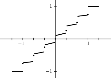
Figure 5 : The solution of (1.3 p = ∞ 𝑝 p=\infty n = 4 𝑛 4 n=4 u ( x ) 𝑢 𝑥 u(x)
For t = 0 𝑡 0 t=0
v k ( 0 ) = 1 2 { f l ( 0 ) + v 2 ( 0 ) , for k = 1 , v k − 1 ( 0 ) + v k + 1 ( 0 ) , for k = 2 , … , n , v n ( 0 ) + f r ( 1 ) , for k = n + 1 . subscript 𝑣 𝑘 0 1 2 cases subscript 𝑓 𝑙 0 subscript 𝑣 2 0 for k = 1 , subscript 𝑣 𝑘 1 0 subscript 𝑣 𝑘 1 0 for k = 2 , … , n , subscript 𝑣 𝑛 0 subscript 𝑓 𝑟 1 for k = n + 1 . v_{k}(0)=\frac{1}{2}\begin{cases}f_{l}(0)+v_{2}(0),\qquad&\text{for $k=1$,}\\
v_{k-1}(0)+v_{k+1}(0),&\text{for $k=2,\dots,n$,}\\
v_{n}(0)+f_{r}(1),\qquad&\text{for $k=n+1$.}\end{cases}
If we define
𝐯 ^ 0 := [ v 1 ( 0 ) , … , v n ( 0 ) , v n + 1 ( 0 ) ] ⊤ ∈ ℝ n + 1 , L ^ := [ 𝟎 ⊤ 0 I n 𝟎 ] ∈ ℝ ( n + 1 ) × ( n + 1 ) , formulae-sequence assign subscript ^ 𝐯 0 superscript subscript 𝑣 1 0 … subscript 𝑣 𝑛 0 subscript 𝑣 𝑛 1 0
top superscript ℝ 𝑛 1 assign ^ 𝐿 matrix superscript 0 top 0 subscript 𝐼 𝑛 0 superscript ℝ 𝑛 1 𝑛 1 \hat{\mathbf{v}}_{0}:=[v_{1}(0),\dots,v_{n}(0),v_{n+1}(0)]^{\top}\in\mathbb{R}^{n+1},\qquad\hat{L}:=\begin{bmatrix}\bf 0^{\top}&0\\
I_{n}&\bf 0\end{bmatrix}\in\mathbb{R}^{(n+1)\times(n+1)},
we get the same equation for 𝐯 ^ 0 subscript ^ 𝐯 0 \hat{\mathbf{v}}_{0} 𝐯 ( t ) 𝐯 𝑡 \mathbf{v}(t)
𝐯 ^ 0 = ∑ k = 1 n + 1 [ ( 1 − k n + 2 ) f l ( 0 ) + k n + 2 f r ( 1 ) ] 𝐞 ^ k . subscript ^ 𝐯 0 superscript subscript 𝑘 1 𝑛 1 delimited-[] 1 𝑘 𝑛 2 subscript 𝑓 𝑙 0 𝑘 𝑛 2 subscript 𝑓 𝑟 1 subscript ^ 𝐞 𝑘 \hat{\mathbf{v}}_{0}=\sum_{k=1}^{n+1}\left[\left(1-\frac{k}{n+2}\right)f_{l}(0)+\frac{k}{n+2}f_{r}(1)\right]\hat{\mathbf{e}}_{k}.
Figure 5
u ( x ) = 1 2 ( u ( x − 1 / 2 ) + u ( x + 1 / 2 ) ) , x ∈ [ − 1 , 1 ] , formulae-sequence 𝑢 𝑥 1 2 𝑢 𝑥 1 2 𝑢 𝑥 1 2 𝑥 1 1 u(x)=\frac{1}{2}\big{(}u(x-1/2)+u(x+1/2)\big{)},\qquad x\in[-1,1],
with boundary values
u ( x ) = { 1 8 sin ( 4 π ( x + 3 / 2 ) ) − 1 , x ∈ [ − 3 / 2 , − 1 ) , 9 8 − x − 1 2 , x ∈ ( 1 , 3 / 2 ] . 𝑢 𝑥 cases 1 8 4 𝜋 𝑥 3 2 1 𝑥 3 2 1 9 8 𝑥 1 2 𝑥 1 3 2 u(x)=\begin{cases}\frac{1}{8}\sin\big{(}4\pi(x+3/2)\big{)}-1,\qquad&x\in[-3/2,-1),\\
\frac{9}{8}-\frac{x-1}{2},&x\in(1,3/2].\end{cases}
Notice the jumps lim x → x k − u ( x ) < u ( x k ) < lim x → x k + u ( x ) subscript → 𝑥 superscript subscript 𝑥 𝑘 𝑢 𝑥 𝑢 subscript 𝑥 𝑘 subscript → 𝑥 superscript subscript 𝑥 𝑘 𝑢 𝑥 \lim_{x\to x_{k}^{-}}u(x)<u(x_{k})<\lim_{x\to x_{k}^{+}}u(x)
We now turn to the case 2 ≤ p < ∞ 2 𝑝 2\leq p<\infty k = 0 , … , n + 1 𝑘 0 … 𝑛 1
k=0,\dots,n+1
V k := V k ( 1 ) where V k ( t ) := ∫ 0 t v k ( s ) d s . formulae-sequence assign subscript 𝑉 𝑘 subscript 𝑉 𝑘 1 where
assign subscript 𝑉 𝑘 𝑡 superscript subscript 0 𝑡 subscript 𝑣 𝑘 𝑠 differential-d 𝑠 V_{k}:=V_{k}(1)\qquad\text{where}\qquad V_{k}(t):=\int_{0}^{t}v_{k}(s)\mathrm{\,d}s.
Then
V 0 ( t ) = ∫ 0 t f l ( s ) d s = : F l ( t ) and V n + 1 ( t ) = ∫ 0 t f r ( s ) d s = : F r ( t ) . V_{0}(t)=\int_{0}^{t}f_{l}(s)\mathrm{\,d}s=:F_{l}(t)\qquad\text{and}\qquad V_{n+1}(t)=\int_{0}^{t}f_{r}(s)\mathrm{\,d}s=:F_{r}(t).
The equation can be written as
v k ( t ) subscript 𝑣 𝑘 𝑡 \displaystyle v_{k}(t) = u ( x k + ϵ t ) absent 𝑢 subscript 𝑥 𝑘 italic-ϵ 𝑡 \displaystyle=u(x_{k}+\epsilon t)
= 3 p + 1 ⋅ 1 2 ϵ ∫ x k − 1 + ϵ t x k + 1 + ϵ t u ( y ) d y + p − 2 p + 1 ⋅ 1 2 ( u ( x k − 1 + ϵ t ) + u ( x k + 1 + ϵ t ) ) absent ⋅ 3 𝑝 1 1 2 italic-ϵ superscript subscript subscript 𝑥 𝑘 1 italic-ϵ 𝑡 subscript 𝑥 𝑘 1 italic-ϵ 𝑡 𝑢 𝑦 differential-d 𝑦 ⋅ 𝑝 2 𝑝 1 1 2 𝑢 subscript 𝑥 𝑘 1 italic-ϵ 𝑡 𝑢 subscript 𝑥 𝑘 1 italic-ϵ 𝑡 \displaystyle=\frac{3}{p+1}\cdot\frac{1}{2\epsilon}\int_{x_{k-1}+\epsilon t}^{x_{k+1}+\epsilon t}u(y)\mathrm{\,d}y+\frac{p-2}{p+1}\cdot\frac{1}{2}\Big{(}u(x_{k-1}+\epsilon t)+u(x_{k+1}+\epsilon t)\Big{)}
= 3 p + 1 ⋅ 1 2 ( V k − 1 − V k − 1 ( t ) + V k + V k + 1 ( t ) ) + p − 2 p + 1 ⋅ 1 2 ( v k − 1 ( t ) + v k + 1 ( t ) ) absent ⋅ 3 𝑝 1 1 2 subscript 𝑉 𝑘 1 subscript 𝑉 𝑘 1 𝑡 subscript 𝑉 𝑘 subscript 𝑉 𝑘 1 𝑡 ⋅ 𝑝 2 𝑝 1 1 2 subscript 𝑣 𝑘 1 𝑡 subscript 𝑣 𝑘 1 𝑡 \displaystyle=\frac{3}{p+1}\cdot\frac{1}{2}\Big{(}V_{k-1}-V_{k-1}(t)+V_{k}+V_{k+1}(t)\Big{)}+\frac{p-2}{p+1}\cdot\frac{1}{2}\Big{(}v_{k-1}(t)+v_{k+1}(t)\Big{)}
for k = 1 , … , n 𝑘 1 … 𝑛
k=1,\dots,n v 0 ( t ) = f l ( t ) subscript 𝑣 0 𝑡 subscript 𝑓 𝑙 𝑡 v_{0}(t)=f_{l}(t) 0 ≤ t < 1 0 𝑡 1 0\leq t<1 v n + 1 ( t ) = f r ( t ) subscript 𝑣 𝑛 1 𝑡 subscript 𝑓 𝑟 𝑡 v_{n+1}(t)=f_{r}(t) 0 < t ≤ 1 0 𝑡 1 0<t\leq 1
𝐕 ′ ( t ) superscript 𝐕 ′ 𝑡 \displaystyle\mathbf{V}^{\prime}(t) = 𝐯 ( t ) absent 𝐯 𝑡 \displaystyle=\mathbf{v}(t)
= 3 p + 1 ⋅ 1 2 ( ( L ⊤ − L ) 𝐕 ( t ) + F r ( t ) 𝐞 n − F l ( t ) 𝐞 1 + ( L + I ) 𝐕 + F l 𝐞 1 ) absent ⋅ 3 𝑝 1 1 2 superscript 𝐿 top 𝐿 𝐕 𝑡 subscript 𝐹 𝑟 𝑡 subscript 𝐞 𝑛 subscript 𝐹 𝑙 𝑡 subscript 𝐞 1 𝐿 𝐼 𝐕 subscript 𝐹 𝑙 subscript 𝐞 1 \displaystyle=\frac{3}{p+1}\cdot\frac{1}{2}\left((L^{\top}-L)\mathbf{V}(t)+F_{r}(t)\mathbf{e}_{n}-F_{l}(t)\mathbf{e}_{1}+(L+I)\mathbf{V}+F_{l}\mathbf{e}_{1}\right)
+ p − 2 p + 1 ⋅ 1 2 ( ( L + L ⊤ ) 𝐕 ′ ( t ) + f l ( t ) 𝐞 1 + f r ( t ) 𝐞 n ) . ⋅ 𝑝 2 𝑝 1 1 2 𝐿 superscript 𝐿 top superscript 𝐕 ′ 𝑡 subscript 𝑓 𝑙 𝑡 subscript 𝐞 1 subscript 𝑓 𝑟 𝑡 subscript 𝐞 𝑛 \displaystyle\qquad{}+\frac{p-2}{p+1}\cdot\frac{1}{2}\left((L+L^{\top})\mathbf{V}^{\prime}(t)+f_{l}(t)\mathbf{e}_{1}+f_{r}(t)\mathbf{e}_{n}\right).
That is,
E p 𝐕 ′ ( t ) = A 𝐕 ( t ) + 𝐅 ( t ) + 1 2 ( L + I ) 𝐕 , 0 < t < 1 , formulae-sequence subscript 𝐸 𝑝 superscript 𝐕 ′ 𝑡 𝐴 𝐕 𝑡 𝐅 𝑡 1 2 𝐿 𝐼 𝐕 0 𝑡 1 E_{p}\mathbf{V}^{\prime}(t)=A\mathbf{V}(t)+\mathbf{F}(t)+\frac{1}{2}(L+I)\mathbf{V},\qquad 0<t<1, (3.2)
where
E p := 1 3 ( ( p + 1 ) I − p − 2 2 ( L + L ⊤ ) ) , assign subscript 𝐸 𝑝 1 3 𝑝 1 𝐼 𝑝 2 2 𝐿 superscript 𝐿 top E_{p}:=\frac{1}{3}\left((p+1)I-\frac{p-2}{2}(L+L^{\top})\right),
and where
𝐅 ( t ) := 1 2 ( ( F l ( 1 ) − F l ( t ) ) 𝐞 1 + F r ( t ) 𝐞 n ) + p − 2 6 ( f l ( t ) 𝐞 1 + f r ( t ) 𝐞 n ) . assign 𝐅 𝑡 1 2 subscript 𝐹 𝑙 1 subscript 𝐹 𝑙 𝑡 subscript 𝐞 1 subscript 𝐹 𝑟 𝑡 subscript 𝐞 𝑛 𝑝 2 6 subscript 𝑓 𝑙 𝑡 subscript 𝐞 1 subscript 𝑓 𝑟 𝑡 subscript 𝐞 𝑛 \mathbf{F}(t):=\frac{1}{2}\left(\big{(}F_{l}(1)-F_{l}(t)\big{)}\mathbf{e}_{1}+F_{r}(t)\mathbf{e}_{n}\right)+\frac{p-2}{6}\left(f_{l}(t)\mathbf{e}_{1}+f_{r}(t)\mathbf{e}_{n}\right).
The matrix E p subscript 𝐸 𝑝 E_{p} 𝐕 ( t ) 𝐕 𝑡 \mathbf{V}(t) 𝐕 ( 0 ) = 0 𝐕 0 0 \mathbf{V}(0)=0 3.2
𝐕 ( t ) 𝐕 𝑡 \displaystyle\mathbf{V}(t) = e t E p − 1 A ( 0 + ∫ 0 t e − s E p − 1 A E p − 1 [ 𝐅 ( s ) + 1 2 ( L + I ) 𝐕 ] d s ) absent superscript 𝑒 𝑡 superscript subscript 𝐸 𝑝 1 𝐴 0 superscript subscript 0 𝑡 superscript 𝑒 𝑠 superscript subscript 𝐸 𝑝 1 𝐴 superscript subscript 𝐸 𝑝 1 delimited-[] 𝐅 𝑠 1 2 𝐿 𝐼 𝐕 differential-d 𝑠 \displaystyle=e^{tE_{p}^{-1}A}\left(0+\int_{0}^{t}e^{-sE_{p}^{-1}A}E_{p}^{-1}\left[\mathbf{F}(s)+\frac{1}{2}(L+I)\mathbf{V}\right]\mathrm{\,d}s\right) (3.3)
= e t E p − 1 A ∫ 0 t e − s E p − 1 A E p − 1 𝐅 ( s ) d s + 1 2 ( e t E p − 1 A − I ) A − 1 ( L + I ) 𝐕 . absent superscript 𝑒 𝑡 superscript subscript 𝐸 𝑝 1 𝐴 superscript subscript 0 𝑡 superscript 𝑒 𝑠 superscript subscript 𝐸 𝑝 1 𝐴 superscript subscript 𝐸 𝑝 1 𝐅 𝑠 differential-d 𝑠 1 2 superscript 𝑒 𝑡 superscript subscript 𝐸 𝑝 1 𝐴 𝐼 superscript 𝐴 1 𝐿 𝐼 𝐕 \displaystyle=e^{tE_{p}^{-1}A}\int_{0}^{t}e^{-sE_{p}^{-1}A}E_{p}^{-1}\mathbf{F}(s)\mathrm{\,d}s+\frac{1}{2}\left(e^{tE_{p}^{-1}A}-I\right)A^{-1}(L+I)\mathbf{V}.
This gives the linear equation
[ I − 1 2 ( e E p − 1 A − I ) A − 1 ( L + I ) ] 𝐕 = e E p − 1 A ∫ 0 1 e − s E p − 1 A E p − 1 𝐅 ( s ) d s delimited-[] 𝐼 1 2 superscript 𝑒 superscript subscript 𝐸 𝑝 1 𝐴 𝐼 superscript 𝐴 1 𝐿 𝐼 𝐕 superscript 𝑒 superscript subscript 𝐸 𝑝 1 𝐴 superscript subscript 0 1 superscript 𝑒 𝑠 superscript subscript 𝐸 𝑝 1 𝐴 superscript subscript 𝐸 𝑝 1 𝐅 𝑠 differential-d 𝑠 \left[I-\frac{1}{2}\left(e^{E_{p}^{-1}A}-I\right)A^{-1}(L+I)\right]\mathbf{V}=e^{E_{p}^{-1}A}\int_{0}^{1}e^{-sE_{p}^{-1}A}E_{p}^{-1}\mathbf{F}(s)\mathrm{\,d}s (3.4)
for 𝐕 = 𝐕 ( 1 ) 𝐕 𝐕 1 \mathbf{V}=\mathbf{V}(1)
2 A [ I − 1 2 ( e E p − 1 A − I ) A − 1 ( L + I ) ] ( L ⊤ + I ) − 1 = I − e A E p − 1 B ~ 2 𝐴 delimited-[] 𝐼 1 2 superscript 𝑒 superscript subscript 𝐸 𝑝 1 𝐴 𝐼 superscript 𝐴 1 𝐿 𝐼 superscript superscript 𝐿 top 𝐼 1 𝐼 superscript 𝑒 𝐴 superscript subscript 𝐸 𝑝 1 ~ 𝐵 2A\left[I-\frac{1}{2}\left(e^{E_{p}^{-1}A}-I\right)A^{-1}(L+I)\right](L^{\top}+I)^{-1}=I-e^{AE_{p}^{-1}}\tilde{B}
and the question of solvability of (3.4 p 𝑝 p 𝐯 0 subscript 𝐯 0 \mathbf{v}_{0}
The formula for u 𝑢 u ( x k , x k + 1 ) subscript 𝑥 𝑘 subscript 𝑥 𝑘 1 (x_{k},x_{k+1}) 3.2
𝐯 ( t ) = E p − 1 ( A 𝐕 ( t ) + 𝐅 ( t ) + 1 2 ( L + I ) 𝐕 ) , 0 < t < 1 . formulae-sequence 𝐯 𝑡 superscript subscript 𝐸 𝑝 1 𝐴 𝐕 𝑡 𝐅 𝑡 1 2 𝐿 𝐼 𝐕 0 𝑡 1 \mathbf{v}(t)=E_{p}^{-1}\left(A\mathbf{V}(t)+\mathbf{F}(t)+\frac{1}{2}(L+I)\mathbf{V}\right),\qquad 0<t<1.
When t = 0 𝑡 0 t=0
v k ( 0 ) = 3 p + 1 ⋅ 1 2 ( V k − 1 + V k ) + p − 2 p + 1 ⋅ 1 2 ( v k − 1 ( 0 ) + v k + 1 ( 0 ) ) subscript 𝑣 𝑘 0 ⋅ 3 𝑝 1 1 2 subscript 𝑉 𝑘 1 subscript 𝑉 𝑘 ⋅ 𝑝 2 𝑝 1 1 2 subscript 𝑣 𝑘 1 0 subscript 𝑣 𝑘 1 0 v_{k}(0)=\frac{3}{p+1}\cdot\frac{1}{2}\Big{(}V_{k-1}+V_{k}\Big{)}+\frac{p-2}{p+1}\cdot\frac{1}{2}\Big{(}v_{k-1}(0)+v_{k+1}(0)\Big{)}
for k = 1 , … , n 𝑘 1 … 𝑛
k=1,\dots,n
v 1 ( 0 ) = 3 p + 1 ⋅ 1 2 ( F l ( 1 ) + V 1 ) + p − 2 p + 1 ⋅ 1 2 ( f l ( 0 ) + v 2 ( 0 ) ) , subscript 𝑣 1 0 ⋅ 3 𝑝 1 1 2 subscript 𝐹 𝑙 1 subscript 𝑉 1 ⋅ 𝑝 2 𝑝 1 1 2 subscript 𝑓 𝑙 0 subscript 𝑣 2 0 v_{1}(0)=\frac{3}{p+1}\cdot\frac{1}{2}\Big{(}F_{l}(1)+V_{1}\Big{)}+\frac{p-2}{p+1}\cdot\frac{1}{2}\Big{(}f_{l}(0)+v_{2}(0)\Big{)},
and
v n + 1 ( 0 ) = 3 p + 1 ⋅ 1 2 ( V n + F r ( 1 ) ) + p − 2 p + 1 ⋅ 1 2 ( v n ( 0 ) + f r ( 1 ) ) . subscript 𝑣 𝑛 1 0 ⋅ 3 𝑝 1 1 2 subscript 𝑉 𝑛 subscript 𝐹 𝑟 1 ⋅ 𝑝 2 𝑝 1 1 2 subscript 𝑣 𝑛 0 subscript 𝑓 𝑟 1 v_{n+1}(0)=\frac{3}{p+1}\cdot\frac{1}{2}\Big{(}V_{n}+F_{r}(1)\Big{)}+\frac{p-2}{p+1}\cdot\frac{1}{2}\Big{(}v_{n}(0)+f_{r}(1)\Big{)}.
We set
Q := [ I 𝟎 ⊤ ] ∈ ℝ ( n + 1 ) × n , assign 𝑄 matrix 𝐼 superscript 0 top superscript ℝ 𝑛 1 𝑛 Q:=\begin{bmatrix}I\\
\bf 0^{\top}\end{bmatrix}\in\mathbb{R}^{(n+1)\times n},
and get the solvable equation
E ^ p 𝐯 ^ 0 = 1 2 ( L ^ + I ^ ) Q 𝐕 + 1 2 ( F l ( 1 ) 𝐞 ^ 1 + F r ( 1 ) 𝐞 ^ n + 1 ) + p − 2 6 ( f l ( 0 ) 𝐞 ^ 1 + f r ( 1 ) 𝐞 ^ n + 1 ) subscript ^ 𝐸 𝑝 subscript ^ 𝐯 0 1 2 ^ 𝐿 ^ 𝐼 𝑄 𝐕 1 2 subscript 𝐹 𝑙 1 subscript ^ 𝐞 1 subscript 𝐹 𝑟 1 subscript ^ 𝐞 𝑛 1 𝑝 2 6 subscript 𝑓 𝑙 0 subscript ^ 𝐞 1 subscript 𝑓 𝑟 1 subscript ^ 𝐞 𝑛 1 \hat{E}_{p}\hat{\mathbf{v}}_{0}=\frac{1}{2}\Big{(}\hat{L}+\hat{I}\Big{)}Q\mathbf{V}+\frac{1}{2}\big{(}F_{l}(1)\hat{\mathbf{e}}_{1}+F_{r}(1)\hat{\mathbf{e}}_{n+1}\big{)}+\frac{p-2}{6}\big{(}f_{l}(0)\hat{\mathbf{e}}_{1}+f_{r}(1)\hat{\mathbf{e}}_{n+1}\big{)}
for 𝐯 ^ 0 := [ v 1 ( 0 ) , … , v n + 1 ( 0 ) ] ⊤ assign subscript ^ 𝐯 0 superscript subscript 𝑣 1 0 … subscript 𝑣 𝑛 1 0
top \hat{\mathbf{v}}_{0}:=[v_{1}(0),\dots,v_{n+1}(0)]^{\top} ℝ n + 1 superscript ℝ 𝑛 1 \mathbb{R}^{n+1}
Figure 6 : The solution of (1.3 p = 5 𝑝 5 p=5 n = 4 𝑛 4 n=4 ± 1 plus-or-minus 1 \pm 1
Some simplifications can be made when the boundary values are constant. If f l ( t ) = − 1 subscript 𝑓 𝑙 𝑡 1 f_{l}(t)=-1 f r ( t ) = 1 subscript 𝑓 𝑟 𝑡 1 f_{r}(t)=1
𝐅 ( t ) 𝐅 𝑡 \displaystyle\mathbf{F}(t) = 1 2 ( ( F l − F l ( t ) ) 𝐞 1 + F r ( t ) 𝐞 n ) + p − 2 6 ( f l ( t ) 𝐞 1 + f r ( t ) 𝐞 n ) absent 1 2 subscript 𝐹 𝑙 subscript 𝐹 𝑙 𝑡 subscript 𝐞 1 subscript 𝐹 𝑟 𝑡 subscript 𝐞 𝑛 𝑝 2 6 subscript 𝑓 𝑙 𝑡 subscript 𝐞 1 subscript 𝑓 𝑟 𝑡 subscript 𝐞 𝑛 \displaystyle=\frac{1}{2}\left(\big{(}F_{l}-F_{l}(t)\big{)}\mathbf{e}_{1}+F_{r}(t)\mathbf{e}_{n}\right)+\frac{p-2}{6}\left(f_{l}(t)\mathbf{e}_{1}+f_{r}(t)\mathbf{e}_{n}\right)
= t 2 ( 𝐞 1 + 𝐞 n ) + p − 2 6 𝐞 n − p + 1 6 𝐞 1 absent 𝑡 2 subscript 𝐞 1 subscript 𝐞 𝑛 𝑝 2 6 subscript 𝐞 𝑛 𝑝 1 6 subscript 𝐞 1 \displaystyle=\frac{t}{2}(\mathbf{e}_{1}+\mathbf{e}_{n})+\frac{p-2}{6}\mathbf{e}_{n}-\frac{p+1}{6}\mathbf{e}_{1}
= t 2 ( 𝐞 1 + 𝐞 n ) + p − 2 6 ( 𝐞 n − 𝐞 1 ) + 1 2 ( L + I ) 𝐞 ~ , absent 𝑡 2 subscript 𝐞 1 subscript 𝐞 𝑛 𝑝 2 6 subscript 𝐞 𝑛 subscript 𝐞 1 1 2 𝐿 𝐼 ~ 𝐞 \displaystyle=\frac{t}{2}(\mathbf{e}_{1}+\mathbf{e}_{n})+\frac{p-2}{6}(\mathbf{e}_{n}-\mathbf{e}_{1})+\frac{1}{2}(L+I)\tilde{\mathbf{e}},
and an integration by parts,
∫ 0 t s e − s E p − 1 A E p − 1 d s superscript subscript 0 𝑡 𝑠 superscript 𝑒 𝑠 superscript subscript 𝐸 𝑝 1 𝐴 superscript subscript 𝐸 𝑝 1 differential-d 𝑠 \displaystyle\int_{0}^{t}se^{-sE_{p}^{-1}A}E_{p}^{-1}\mathrm{\,d}s = − | 0 t s e − s E p − 1 A ( E p − 1 A ) − 1 E p − 1 + ∫ 0 t e − s E p − 1 A ( E p − 1 A ) − 1 E p − 1 d s \displaystyle=-\bigg{|}_{0}^{t}se^{-sE_{p}^{-1}A}(E_{p}^{-1}A)^{-1}E_{p}^{-1}+\int_{0}^{t}e^{-sE_{p}^{-1}A}(E_{p}^{-1}A)^{-1}E_{p}^{-1}\mathrm{\,d}s
= − t e − t E p − 1 A A − 1 − ( e − t E p − 1 A − I ) A − 1 E p A − 1 , absent 𝑡 superscript 𝑒 𝑡 superscript subscript 𝐸 𝑝 1 𝐴 superscript 𝐴 1 superscript 𝑒 𝑡 superscript subscript 𝐸 𝑝 1 𝐴 𝐼 superscript 𝐴 1 subscript 𝐸 𝑝 superscript 𝐴 1 \displaystyle=-te^{-tE_{p}^{-1}A}A^{-1}-\left(e^{-tE_{p}^{-1}A}-I\right)A^{-1}E_{p}A^{-1},
yields
𝐕 ( t ) 𝐕 𝑡 \displaystyle\mathbf{V}(t) = e t E p − 1 A ∫ 0 t e − s E p − 1 A E p − 1 [ s 2 ( 𝐞 1 + 𝐞 n ) + p − 2 6 ( 𝐞 n − 𝐞 1 ) + 1 2 ( L + I ) ( 𝐕 + 𝐞 ~ ) ] d s absent superscript 𝑒 𝑡 superscript subscript 𝐸 𝑝 1 𝐴 superscript subscript 0 𝑡 superscript 𝑒 𝑠 superscript subscript 𝐸 𝑝 1 𝐴 superscript subscript 𝐸 𝑝 1 delimited-[] 𝑠 2 subscript 𝐞 1 subscript 𝐞 𝑛 𝑝 2 6 subscript 𝐞 𝑛 subscript 𝐞 1 1 2 𝐿 𝐼 𝐕 ~ 𝐞 differential-d 𝑠 \displaystyle=e^{tE_{p}^{-1}A}\int_{0}^{t}e^{-sE_{p}^{-1}A}E_{p}^{-1}\Big{[}\tfrac{s}{2}(\mathbf{e}_{1}+\mathbf{e}_{n})+\tfrac{p-2}{6}(\mathbf{e}_{n}-\mathbf{e}_{1})+\tfrac{1}{2}(L+I)(\mathbf{V}+\tilde{\mathbf{e}})\Big{]}\mathrm{\,d}s
= e t E p − 1 A ( − t e − t E p − 1 A A − 1 − ( e − t E p − 1 A − I ) A − 1 E p A − 1 ) 1 2 ( 𝐞 1 + 𝐞 n ) absent superscript 𝑒 𝑡 superscript subscript 𝐸 𝑝 1 𝐴 𝑡 superscript 𝑒 𝑡 superscript subscript 𝐸 𝑝 1 𝐴 superscript 𝐴 1 superscript 𝑒 𝑡 superscript subscript 𝐸 𝑝 1 𝐴 𝐼 superscript 𝐴 1 subscript 𝐸 𝑝 superscript 𝐴 1 1 2 subscript 𝐞 1 subscript 𝐞 𝑛 \displaystyle=e^{tE_{p}^{-1}A}\left(-te^{-tE_{p}^{-1}A}A^{-1}-\left(e^{-tE_{p}^{-1}A}-I\right)A^{-1}E_{p}A^{-1}\right)\frac{1}{2}(\mathbf{e}_{1}+\mathbf{e}_{n})
+ e t E p − 1 A ∫ 0 t e − s E p − 1 A E p − 1 [ p − 2 6 ( 𝐞 n − 𝐞 1 ) + 1 2 ( L + I ) ( 𝐕 + 𝐞 ~ ) ] d s superscript 𝑒 𝑡 superscript subscript 𝐸 𝑝 1 𝐴 superscript subscript 0 𝑡 superscript 𝑒 𝑠 superscript subscript 𝐸 𝑝 1 𝐴 superscript subscript 𝐸 𝑝 1 delimited-[] 𝑝 2 6 subscript 𝐞 𝑛 subscript 𝐞 1 1 2 𝐿 𝐼 𝐕 ~ 𝐞 differential-d 𝑠 \displaystyle\qquad{}+e^{tE_{p}^{-1}A}\int_{0}^{t}e^{-sE_{p}^{-1}A}E_{p}^{-1}\left[\frac{p-2}{6}(\mathbf{e}_{n}-\mathbf{e}_{1})+\frac{1}{2}(L+I)\big{(}\mathbf{V}+\tilde{\mathbf{e}}\big{)}\right]\mathrm{\,d}s
= − ( t I + ( I − e t E p − 1 A ) A − 1 E p ) 𝐞 ~ absent 𝑡 𝐼 𝐼 superscript 𝑒 𝑡 superscript subscript 𝐸 𝑝 1 𝐴 superscript 𝐴 1 subscript 𝐸 𝑝 ~ 𝐞 \displaystyle=-\left(tI+\left(I-e^{tE_{p}^{-1}A}\right)A^{-1}E_{p}\right)\tilde{\mathbf{e}}
− ( I − e t E p − 1 A ) A − 1 ( p − 2 6 ( 𝐞 n − 𝐞 1 ) + 1 2 ( L + I ) ( 𝐕 + 𝐞 ~ ) ) 𝐼 superscript 𝑒 𝑡 superscript subscript 𝐸 𝑝 1 𝐴 superscript 𝐴 1 𝑝 2 6 subscript 𝐞 𝑛 subscript 𝐞 1 1 2 𝐿 𝐼 𝐕 ~ 𝐞 \displaystyle\qquad{}-\left(I-e^{tE_{p}^{-1}A}\right)A^{-1}\left(\frac{p-2}{6}(\mathbf{e}_{n}-\mathbf{e}_{1})+\frac{1}{2}(L+I)\big{(}\mathbf{V}+\tilde{\mathbf{e}}\big{)}\right)
= ( e t E p − 1 A − I ) A − 1 ( p − 2 6 ( 𝐞 n − 𝐞 1 ) + 1 2 ( L + I ) ( 𝐕 + 𝐞 ~ ) + E p 𝐞 ~ ) − t 𝐞 ~ . absent superscript 𝑒 𝑡 superscript subscript 𝐸 𝑝 1 𝐴 𝐼 superscript 𝐴 1 𝑝 2 6 subscript 𝐞 𝑛 subscript 𝐞 1 1 2 𝐿 𝐼 𝐕 ~ 𝐞 subscript 𝐸 𝑝 ~ 𝐞 𝑡 ~ 𝐞 \displaystyle=\left(e^{tE_{p}^{-1}A}-I\right)A^{-1}\left(\frac{p-2}{6}(\mathbf{e}_{n}-\mathbf{e}_{1})+\frac{1}{2}(L+I)\big{(}\mathbf{V}+\tilde{\mathbf{e}}\big{)}+E_{p}\tilde{\mathbf{e}}\right)-t\tilde{\mathbf{e}}.
The equation for 𝐕 + 𝐞 ~ 𝐕 ~ 𝐞 \mathbf{V}+\tilde{\mathbf{e}}
[ I − 1 2 ( e E p − 1 A − I ) A − 1 ( L + I ) ] ( 𝐕 + 𝐞 ~ ) delimited-[] 𝐼 1 2 superscript 𝑒 superscript subscript 𝐸 𝑝 1 𝐴 𝐼 superscript 𝐴 1 𝐿 𝐼 𝐕 ~ 𝐞 \displaystyle\left[I-\tfrac{1}{2}\left(e^{E_{p}^{-1}A}-I\right)A^{-1}(L+I)\right]\big{(}\mathbf{V}+\tilde{\mathbf{e}}\big{)} = ( e E p − 1 A − I ) A − 1 ( p − 2 6 ( 𝐞 n − 𝐞 1 ) + E p 𝐞 ~ ) , absent superscript 𝑒 superscript subscript 𝐸 𝑝 1 𝐴 𝐼 superscript 𝐴 1 𝑝 2 6 subscript 𝐞 𝑛 subscript 𝐞 1 subscript 𝐸 𝑝 ~ 𝐞 \displaystyle=\left(e^{E_{p}^{-1}A}-I\right)A^{-1}\left(\tfrac{p-2}{6}(\mathbf{e}_{n}-\mathbf{e}_{1})+E_{p}\tilde{\mathbf{e}}\right),
and a differentiation gives
𝐯 ( t ) = 𝐕 ′ ( t ) = e t E p − 1 A ( p − 2 6 E p − 1 ( 𝐞 n − 𝐞 1 ) + 1 2 E p − 1 ( L + I ) ( 𝐕 + 𝐞 ~ ) + 𝐞 ~ ) − 𝐞 ~ . 𝐯 𝑡 superscript 𝐕 ′ 𝑡 superscript 𝑒 𝑡 superscript subscript 𝐸 𝑝 1 𝐴 𝑝 2 6 superscript subscript 𝐸 𝑝 1 subscript 𝐞 𝑛 subscript 𝐞 1 1 2 superscript subscript 𝐸 𝑝 1 𝐿 𝐼 𝐕 ~ 𝐞 ~ 𝐞 ~ 𝐞 \mathbf{v}(t)=\mathbf{V}^{\prime}(t)=e^{tE_{p}^{-1}A}\left(\frac{p-2}{6}E_{p}^{-1}(\mathbf{e}_{n}-\mathbf{e}_{1})+\frac{1}{2}E_{p}^{-1}(L+I)\big{(}\mathbf{V}+\tilde{\mathbf{e}}\big{)}+\tilde{\mathbf{e}}\right)-\tilde{\mathbf{e}}.
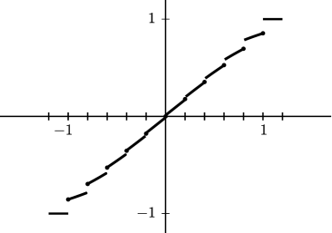
Figure 7 : p = 100 𝑝 100 p=100 and n = 6 𝑛 6 n=6 ± 1 plus-or-minus 1 \pm 1
Finally, the equation for the values 𝐯 ^ 0 := [ v 1 ( 0 ) , … , v n + 1 ( 0 ) ] ⊤ assign subscript ^ 𝐯 0 superscript subscript 𝑣 1 0 … subscript 𝑣 𝑛 1 0
top \hat{\mathbf{v}}_{0}:=[v_{1}(0),\dots,v_{n+1}(0)]^{\top}
E ^ p 𝐯 ^ 0 subscript ^ 𝐸 𝑝 subscript ^ 𝐯 0 \displaystyle\hat{E}_{p}\hat{\mathbf{v}}_{0} = 1 2 ( L ^ + I ^ ) Q 𝐕 + 1 2 ( F l ( 1 ) 𝐞 ^ 1 + F r ( 1 ) 𝐞 ^ n + 1 ) + p − 2 6 ( f l ( 0 ) 𝐞 ^ 1 + f r ( 1 ) 𝐞 ^ n + 1 ) absent 1 2 ^ 𝐿 ^ 𝐼 𝑄 𝐕 1 2 subscript 𝐹 𝑙 1 subscript ^ 𝐞 1 subscript 𝐹 𝑟 1 subscript ^ 𝐞 𝑛 1 𝑝 2 6 subscript 𝑓 𝑙 0 subscript ^ 𝐞 1 subscript 𝑓 𝑟 1 subscript ^ 𝐞 𝑛 1 \displaystyle=\frac{1}{2}\Big{(}\hat{L}+\hat{I}\Big{)}Q\mathbf{V}+\frac{1}{2}\big{(}F_{l}(1)\hat{\mathbf{e}}_{1}+F_{r}(1)\hat{\mathbf{e}}_{n+1}\big{)}+\frac{p-2}{6}\big{(}f_{l}(0)\hat{\mathbf{e}}_{1}+f_{r}(1)\hat{\mathbf{e}}_{n+1}\big{)}
= 1 2 ( L ^ + I ^ ) Q 𝐕 + p + 1 6 ( 𝐞 ^ n + 1 − 𝐞 ^ 1 ) . absent 1 2 ^ 𝐿 ^ 𝐼 𝑄 𝐕 𝑝 1 6 subscript ^ 𝐞 𝑛 1 subscript ^ 𝐞 1 \displaystyle=\frac{1}{2}\Big{(}\hat{L}+\hat{I}\Big{)}Q\mathbf{V}+\frac{p+1}{6}\big{(}\hat{\mathbf{e}}_{n+1}-\hat{\mathbf{e}}_{1}\big{)}.
The Figures 6 8 1.3 n 𝑛 n p 𝑝 p p → ∞ → 𝑝 p\to\infty
Figure 8 : p = 25 𝑝 25 p=25 and n = 10 𝑛 10 n=10 ± 1 plus-or-minus 1 \pm 1
When p > 2 𝑝 2 p>2 E p − 1 A superscript subscript 𝐸 𝑝 1 𝐴 E_{p}^{-1}A e t E p − 1 A superscript 𝑒 𝑡 superscript subscript 𝐸 𝑝 1 𝐴 e^{tE_{p}^{-1}A} E p subscript 𝐸 𝑝 E_{p} E p − 1 A superscript subscript 𝐸 𝑝 1 𝐴 E_{p}^{-1}A e t E p − 1 A superscript 𝑒 𝑡 superscript subscript 𝐸 𝑝 1 𝐴 e^{tE_{p}^{-1}A} cos ( λ t ) + i sin ( λ t ) 𝜆 𝑡 𝑖 𝜆 𝑡 \cos(\lambda t)+i\sin(\lambda t) 2 < p < ∞ 2 𝑝 2<p<\infty