Nuclear charge-exchange excitations based on relativistic density-dependent point-coupling model

Abstract

Spin-isospin transitions in nuclei away from the valley of stability are essential for the description of astrophysically relevant weak interaction processes. While they remain mainly beyond the reach of experiment, theoretical modeling provides important insight into their properties. In order to describe the spin-isospin response, the proton-neutron relativistic quasiparticle random phase approximation (PN-RQRPA) is formulated using the relativistic density-dependent point coupling interaction, and separable pairing interaction in both the $T=1$ and $T=0$ pairing channels. By implementing recently established DD-PCX interaction with improved isovector properties relevant for the description of nuclei with neutron-to-proton number asymmetry, the isobaric analog resonances (IAR) and Gamow-Teller resonances (GTR) have been investigated. In contrast to other models that usually underestimate the IAR excitation energies in Sn isotope chain, the present model accurately reproduces the experimental data, while the GTR properties depend on the isoscalar pairing interaction strength. This framework provides not only an improved description of the spin-isospin response in nuclei, but it also allows future large scale calculations of charge-exchange excitations and weak interaction processes in stellar environment.

I Introduction

Charge-exchange excitations in atomic nuclei correspond to a class of nuclear transitions composed of the particle-hole configurations that contain the exchange of the nucleon charge, described by the isospin projection lowering (increasing) operator $\tau_{-}$ ($\tau_{+}$). The fundamental charge-exchange excitation is the isobaric analog resonance (IAR) Auerbach et al. (1972); Auerbach (1983); Rumyantsev and Urin (1994); Pham et al. (1995); Colò et al. (1998); Paar et al. (2004); Fracasso and Colò (2005); Roca-Maza et al. (2012), with no changes in quantum numbers $\Delta J=\Delta L=\Delta S=\text{0}$, thus the IAR corresponds to a collective excitation with $J^{\pi}={\text{0}}^{+}$. The Gamow-Teller resonance (GTR) represents another relevant charge-exchange mode, characterized by $J^{\pi}={\text{1}}^{+}$, i.e., it corresponds to spin-flip excitations without changing the orbital motion, $\Delta S=\text{1}$, $\Delta L=\text{0}$.

As it has been emphasized in Ref. Roca-Maza and Paar (2018), recent interest in the GTR studies is motivated by its importance for understanding the spin and spin-isospin dependence of modern effective interactions  Bender et al. (2002); Marketin et al. (2012a); Litvinova et al. (2014); Ekström et al. (2014); Zelevinsky et al. (2017); Morita and Kanada-En’yo (2017); Nabi et al. (2017); Ha and Cheoun (2017), nuclear beta decay Engel et al. (1988); Borzov et al. (1995); Engel et al. (1999); Borzov (2003); Madurga et al. (2016); Marketin et al. (2016); Moon et al. (2017); Wang et al. (2016); Ravlić et al. (2020a), beta delayed neutron emission Caballero-Folch et al. (2016), as well as double beta decay Faessler and Simkovic (1998); Suhonen and Civitarese (1998); Šimkovic et al. (2011); Menéndez et al. (2011); Vergados et al. (2012); Menéndez et al. (2014); Štefánik et al. (2015); Navas-Nicolás and Sarriguren (2015); Delion and Suhonen (2017). In addition, accurate description of GT^± transitions, including both in stable and exotic nuclei, is relevant for the description of a variety of astrophysically relevant weak interaction processes Langanke and Martinez-Pinedo (2000); Langanke and Martínez-Pinedo (2003); Janka et al. (2007); Noji et al. (2014); Paar et al. (2015), electron capture in presupernova stars  Niu et al. (2011, 2013); Ravlić et al. (2020b), r-process Arnould et al. (2007); Mori et al. (2016) and neutrino-nucleus interaction of relevance for neutrino detectors and neutrino nucleosynthesis in stellar environment Ejiri (2000); Suzuki and Sagawa (2003); Frekers et al. (2011); Cheoun et al. (2010); Paar et al. (2008, 2011); Karakoç et al. (2014).

The properties of charge-exchange modes of excitation have extensively been studied  Osterfeld (1992); Fujita et al. (2011). Following theoretical prediction  Ikeda et al. (1963), in 1975 the GTR has been experimentally confirmed in $(p,n)$ reactions Doering et al. (1975). The GTR represents one of the most extensively investigated collective excitation in nuclear physics, both experimentally and theoretically (e.g., see Refs. Osterfeld (1992); Halbleib and Sorensen (1967); Doering et al. (1975); Towner and Khanna (1979); Goodman et al. (1980); Brown and Rho (1981); Bertsch and Hamamoto (1982); Nakayama et al. (1982); Van Giai and Sagawa (1981); Gaarde (1983); Kuzmin and Soloviev (1984); Colò et al. (1994); Hamamoto and Sagawa (1993); Brown and Rykaczewski (1994); Suzuki and Otsuka (1997); De Conti et al. (1998); Caurier et al. (1999); Langanke et al. (2001); Bender et al. (2002); Algora et al. (2003); Kalmykov et al. (2006); Bai et al. (2009); Lutostansky (2011); Sasano et al. (2011); Fujita et al. (2011); Niu et al. (2012); Ha and Cheoun (2013); Roca-Maza et al. (2013); Martini et al. (2014); Ha and Cheoun (2016); Niu et al. (2016); Liang et al. (2018); Yasuda et al. (2018)). More details about experimental studies of spin-isospin excitations are also reviewed in Ref. Fujita et al. (2011). Recent studies of the GTR in the framework based on relativistic energy density functional include relativistic quasiparticle random phase approximation (RQRPA) Paar et al. (2004), the relativistic RPA based on the relativistic Hartree-Fock (RHF) Liang et al. (2008), relativistic QRPA based on point coupling model with nonlinear interactions Niu et al. (2013); Wang et al. (2016), and relativistic QRPA formulated using the relativistic Hatree–Fock–Bogoliubov (RHFB) model for the ground state Niu et al. (2017). In Ref. Finelli et al. (2007) the nuclear density functional framework, based on chiral dynamics and the symmetry breaking pattern of low-energy QCD, has been used to formulate the proton–neutron QRPA to investigate the role of chiral pion–nucleon dynamics in the description of charge-exchange excitations. The GTR has also been studied by including couplings between single nucleon and collective nuclear vibrations, e.g., particle-vibration coupling (PVC) of the 1p-1h$\otimes$phonon type of coupling Niu et al. (2012); Marketin et al. (2012b); Niu et al. (2016); Robin and Litvinova (2019). The PVC allows to include important dynamical correlations missing in the static self-consistent mean field models and it provides additional fragmentation of the GTR strength when compared to the random phase approximation studies based only on 1p-1h configurations Niu et al. (2012).

At present, the knowledge about charge-exchange transitions in nuclei away from the valley of stability is rather limited, and mainly beyond the reach of experiment. Since these nuclei are especially important for their astrophysical relevance in stellar evolution and nucleosynthesis, it is crucial to develop microscopic theoretical approaches, that allow quantitative and systematic analyses of the transition strength distributions of unstable nuclei. In order to assess the overview into systematical model uncertainties in modeling charge-exchange excitation phenomena, it is important to address their properties from various approaches, by implementing different theory frameworks and effective nuclear interactions.

In Ref. Paar et al. (2004) charge-exchange excitations have been studied in the framework based on the relativistic nuclear energy density functional (EDF), within the approach that unifies the treatment of mean-field and pairing correlations, relativistic quasiparticle random phase approximation (RQRPA) formulated in the canonical single-nucleon basis of the relativistic Hartree-Bogoliubov (RHB) model. In this implementation the relativistic EDF with explicit density dependence of the meson-nucleon couplings is used, that provides an improved description of asymmetric nuclear matter, neutron matter and nuclei far from stability. The pairing correlations were described by the pairing part of the finite range Gogny interaction Dechargé and Gogny (1980); Berger et al. (1991). However, the EDFs have usually been parameterized with the experimental data on the ground state properties, supplemented with the pseudo-observables on nuclear matter properties. In the case of density dependent meson-exchange interactions, the neutron skin thickness in ²⁰⁸Pb has been introduced as an additional constraint on the isovector channel of the effective interaction. However, the results from measurements of the neutron-skin thickness are usually model-dependent, and the pseudo-observables on nuclear matter are often rather arbitrary. Recently, a novel EDF parameterization has been established based on the relativistic point coupling interaction, by using in the $\chi^{2}$ minimization the nuclear ground state properties (binding energies, charge radii, pairing gaps) together with the properties of collective excitations in nuclei, isoscalar giant monopole resonance energy and dipole polarizability Yüksel et al. (2019). In this way an effective interaction DD-PCX has been established with improved isovector properties, that is successful not only in the description of nuclear ground state, but also of the excitation phenomena, incompressibility of nuclear matter and the symmetry energy close to the saturation density Yüksel et al. (2019). The improved isovector channel for the DD-PCX interaction is especially important not only for the symmetry energy of the nuclear equation of state, but also for the description of ground-state and excitation properties of $N\neq Z$ nuclei. Clearly, this is very important for the implementation of the EDF based models to exotic nuclei, as well as for applications in nuclear astrophysics.

In this work we establish the proton-neutron RQRPA in the canonical single-nucleon basis of the RHB model based on density-dependent relativistic point coupling interaction. Our study represents the first implementation of the relativistic point coupling interaction with density dependent vertex functions in formulating the RQRPA for the description of charge-exchange excitations. In addition, the treatment of the pairing correlations is also improved, by implementing the separable pairing force that allows accurate and efficient calculations of the pairing properties Tian et al. (2009). By using recently established DD-PCX interaction with improved properties that are essential for description of nuclei away from the valley of stability Yüksel et al. (2019), the proton-neutron RQRPA established in this work will be employed in the investigation of the properties of collective charge-exchange excitations, IAR and GTR.

Clearly, a study of both the IAR and GTR properties represents an important benchmark test for novel theoretical approaches established not only for description of charge-excitation modes, but also for modeling a variety of astrophysically relevant processes in stellar environment. Therefore, in the present work that introduces a microscopic approach to describe charge-exchange excitations based on density-dependent relativistic point coupling interaction, the novel theory framework will be employed in the analyses of charge-exchange modes, the IAR and GTR, both for magic nuclei, as well as for open-shell nuclei to probe the effect of the pairing correlations.

In Sec. II the formalism of the proton-neutron RQRPA based on the density dependent point coupling interaction is introduced. In Sec. III the model is employed in studies of charge-exchange modes of excitation, the IAR and the GTR. The conclusions of this work are summarized in Section IV.

II Proton-neutron RQRPA based on relativistic point coupling interaction

In the previous implementation in the relativistic framework, the RQRPA has been established on the ground of relativistic Hartree-Bogoliubov (RHB) model, based on the effective Lagrangian with density-dependent meson-exchange interaction terms Paar et al. (2004). Therein the pairing correlations have been described by the pairing part of the Gogny interaction Dechargé and Gogny (1980); Berger et al. (1991). In the present study, the RQRPA is established using the relativistic point coupling interaction, while the pairing correlations are described by the separable pairing force from Ref. Tian et al. (2009). Since the full RQRPA equations are rather complicated, in the present study we solve the respective equations in the canonical basis, where the Hartree-Bogoliubov wave functions can be expressed in the form of the BCS-like wave functions. More details on the implementation of the canonical basis in the RHB model and general formalism of the PN-RQRPA equations in the canonical basis are given in Ref. Paar et al. (2004). The focus of this work is the implementation of the relativistic point coupling interaction in deriving the PN-RQRPA equations. The nuclear ground state properties are described in the RHB model for the point coupling interaction, described in detail in Ref. Nikšić et al. (2014).

Starting from the $0^{+}$ ground state of a spherical even-even nucleus, transitions to $J^{\pi}$ excited state of the corresponding odd-odd daughter nucleus are considered, using the charge-exchange operator ${\cal{O}}^{JM}$. The general form of the PN-RQRPA equations read Paar et al. (2004),

$$\left(\begin{array}[c]{cc}A^{J}&B^{J}\\ B^{{}^{\ast}J}&A^{{}^{\ast}J}\end{array}\right)\left(\begin{array}[c]{c}X^{\lambda J}\\ Y^{\lambda J}\end{array}\right)=E_{\lambda}\left(\begin{array}[c]{cc}1&0\\ 0&-1\end{array}\right)\left(\begin{array}[c]{c}X^{\lambda J}\\ Y^{\lambda J}\end{array}\right)\;,$$ (1)

where the $A$ and $B$ matrices are defined in the canonical basis,

$$A_{pn,p^{\prime}n^{\prime}}^{J} = H^{11}_{pp^{\prime}}\delta_{nn^{\prime}}+H^{11}_{nn^{\prime}}\delta_{pp^{\prime}}$$

$$+\left(u_{p}v_{n}u_{p^{\prime}}v_{n^{\prime}}+v_{p}u_{n}v_{p^{\prime}}u_{n^{\prime}}\right)V_{pn^{\prime}np^{\prime}}^{phJ}+\left(u_{p}u_{n}u_{p^{\prime}}u_{n^{\prime}}+v_{p}v_{n}v_{p^{\prime}}v_{n^{\prime}}\right)V_{pnp^{\prime}n^{\prime}}^{ppJ}$$

$$B_{pn,p^{\prime}n^{\prime}}^{J} = \left(u_{p}v_{n}v_{p^{\prime}}u_{n^{\prime}}+v_{p}u_{n}u_{p^{\prime}}v_{n^{\prime}}\right)V_{pn^{\prime}np^{\prime}}^{phJ}$$ (2)

$$-\left(u_{p}u_{n}v_{p^{\prime}}v_{n^{\prime}}+v_{p}v_{n}u_{p^{\prime}}u_{n^{\prime}}\right)V_{pnp^{\prime}n^{\prime}}^{ppJ}\;.$$

The proton and neutron quasiparticle canonical states are denoted by $p$, $p\prime$, and $n$, $n\prime$, respectively. $V^{ph}$ is the proton-neutron particle-hole residual interaction, and $V^{pp}$ is the corresponding particle-particle interaction, and $u$ and $v$ denote the occupation amplitudes of the respective states. Since the canonical basis does not diagonalize the Dirac single-nucleon mean-field Hamiltonian, the off-diagonal matrix elements $H^{11}_{nn^{\prime}}$ and $H^{11}_{pp^{\prime}}$ are also included in the $A$ matrix, as given in Ref. Paar et al. (2004). $E_{\lambda}$ denote the excitation energy, while $X^{\lambda J}$ and $Y^{\lambda J}$ are the corresponding forward- and backward-going QRPA amplitudes, respectively.

By solving the eigenvalue problem (1), the reduced transition strength can be obtained between the ground state of the even-even $(N,Z)$ nucleus and the excited state of the odd-odd $(N+1,Z-1)$ or $(N-1,Z+1)$ nucleus, using the corresponding transition operators ${\cal{O}}^{JM}$ in both channels,

$$B_{\lambda J}^{-}=\left|\sum_{pn}<p||{\cal{O}}^{J}||n>\left(X_{pn}^{\lambda J}u_{p}v_{n}+Y_{pn}^{\lambda J}v_{p}u_{n}\right)\right|^{2}\;,$$ (3)

$$B_{\lambda J}^{+}=\left|\sum_{pn}(-1)^{j_{p}+j_{n}+J}<n||{\cal{O}}^{J}||p>\left(X_{np}^{\lambda J}v_{p}u_{n}+Y_{np}^{\lambda J}u_{p}v_{n}\right)\right|^{2}\;.$$ (4)

For the presentation purposes, the discrete strength distribution is folded by the Lorentzian function of the width $\Gamma=1$ MeV,

$$R(E)^{\pm}=\sum_{\lambda}B_{\lambda J}^{\pm}\frac{1}{\pi}\frac{\Gamma/2}{(E-E_{\lambda_{\pm}})^{2}+(\Gamma/2)^{2}}\;.$$ (5)

In the implementation of the relativistic point coupling interaction, the spin-isospin dependent terms in the residual interaction of the PN-RQRPA are induced by the isovector-vector and pseudovector terms. In comparison, for the finite range meson-exchange interaction, these terms were obtained from the $\rho$-and $\pi$-meson exchange, respectively Paar et al. (2004). In the present study, the PN-RQRPA residual interaction terms $V_{abcd}$ are derived from the effective Lagrangian density for the point coupling interaction.

The isovector-vector part of PN-RQRPA contains only non-rearrangement terms of the residual two-body interaction. For the respective spacelike components we obtain,

$$V_{abcd}^{(\text{TVs})}~{}=~{}-\int d^{3}r_{1}\int d^{3}r_{2}\psi_{a}^{\dagger}(\vec{r}_{1})\left(\vec{\tau}\gamma_{0}\gamma_{i}\right)^{(1)}\psi_{c}(\vec{r}_{1})\alpha_{TV}(\rho)\delta(\vec{r}_{1}-\vec{r}_{2})\psi_{b}^{\dagger}(\vec{r}_{2})\left(\vec{\tau}\gamma_{0}\gamma^{i}\right)^{(2)}\psi_{d}(\vec{r}_{2}),$$ (6)

and timelike components are given by

$$V_{abcd}^{(\text{TVt})}~{}=~{}\int d^{3}r_{1}\int d^{3}r_{2}\psi_{a}^{\dagger}(\vec{r}_{1})\vec{\tau}^{(1)}\psi_{c}(\vec{r}_{1})\alpha_{TV}(\rho)\delta(\vec{r}_{1}-\vec{r}_{2})\psi_{b}^{\dagger}(\vec{r}_{2})\vec{\tau}^{(2)}\psi_{d}(\vec{r}_{2}),$$ (7)

where the coupling $\alpha_{TV}(\rho)$ is a function of baryon (vector) density. For Dirac spinor given by,

$$\psi_{am_{a}}(r)~{}=~{}\left(\begin{array}[]{clcr}f_{a}(r)\Omega_{\kappa_{a}m_{a}}(\Omega)\\ \ ig_{a}(r)\Omega_{\bar{\kappa}_{a}m_{a}}(\Omega)\end{array}\right),$$ (8)

where $a$ stands for all quantum numbers, with the exception of the projection of total angular momentum $m_{a}$. Quantum number $\kappa$ is defined as $\kappa=-(l+1)$ for $j=l+1/2$ and $\kappa=l$ for $j=l-1/2$, while $\bar{l}=2j-l$ corresponds to the lower component orbital angular momentum Greiner and Bromley (2000). The spacelike part of the matrix elements obtained by the angular momentum coupling is given

$$V_{abcd}^{(\text{TVs})J}~{}=~{}\frac{2}{\left(2J+1\right)}\sum_{L}\int drr^{2}\alpha_{TV}(\rho)\bigg{[}f_{a}(r)g_{c}(r)\langle(1/2\ l_{a})j_{a}||\left[\sigma_{S}Y_{L}\right]_{J}||(1/2\ \bar{l}_{c})j_{c}\rangle-$$

$$~{}g_{a}(r)f_{c}(r)\langle(1/2\ \bar{l}_{a})j_{a}||\left[\sigma_{S}Y_{L}\right]_{J}||(1/2\ l_{c})j_{c}\rangle\bigg{]}\bigg{[}f_{b}(r)g_{d}(r)\langle(1/2\ \bar{l}_{d})j_{d}||\left[\sigma_{S}Y_{L}\right]_{J}||(1/2\ l_{b})j_{b}\rangle$$

$$~{}-g_{b}(r)f_{d}(r)\langle(1/2\ l_{d})j_{d}||\left[\sigma_{S}Y_{L}\right]_{J}||(1/2\ \bar{l}_{b})j_{b}\rangle\bigg{]},$$ (9)

and the timelike part is

$$V_{abcd}^{(TVt)J}~{}= ~{}\frac{2}{2J+1}\int drr^{2}\alpha_{TV}(\rho)\bigg{[}f_{a}(r)f_{c}(r)+g_{a}(r)g_{c}(r)\bigg{]}\bigg{[}f_{b}(r)f_{d}(r)+g_{b}(r)g_{d}(r)\bigg{]}$$

$$~{}\times\langle(1/2\ l_{a})j_{a}||Y_{J}||(1/2\ l_{c})j_{c}\rangle\langle(1/2\ l_{d})j_{d}||Y_{J}||(1/2\ l_{b})j_{b}\rangle.$$ (10)

When compared to standard R(Q)RPA matrix elements, in particular corresponding direct term, there exists an additional factor of 2 in the numerator of Eqs. (9) and (10) due to the difference in the isospin part of the matrix element (see Appendix A). The isovector-pseudovector part of the point coupling interaction is given by

$$V_{PV}~{}=~{}-\alpha_{PV}\delta(\vec{r}_{1}-\vec{r}_{2})\left(\gamma_{0}\gamma_{5}\gamma_{\mu}\vec{\tau}\right)^{(1)}\left(\gamma_{0}\gamma_{5}\gamma^{\mu}\vec{\tau}\right)^{(2)},$$ (11)

where $\alpha_{PV}$ denotes the strength parameter of the interaction. Since $\alpha_{PV}$ remains a free parameter of the model that cannot be constrained by the ground state properties, its value should be constrained by the experimental data on charge-exchange excitations. For the corresponding timelike part of the pseudovector matrix elements we obtain,

$$V_{abcd}^{\text{PV(t)J}}~{}= ~{}\frac{2\alpha_{PV}}{2J+1}\int drr^{2}\bigg{[}f_{a}(r)g_{c}(r)-g_{a}(r)f_{c}(r)\bigg{]}\bigg{[}f_{b}(r)g_{d}(r)-g_{b}(r)f_{d}(r)\bigg{]}$$

$$\times\langle(1/2\ l_{a})j_{a}||Y_{J}||(1/2\ \bar{l}_{c})j_{c}\rangle\langle(1/2\ \bar{l}_{d})j_{d}||Y_{J}||(1/2\ l_{c})j_{c}\rangle.$$ (12)

We note that the timelike matrix elements are non-zero only in the case of unnatural parity transitions, e.g., for Gamow-Teller transitions. The spacelike part of the isovector-pseudovector matrix elements results,

$$V_{abcd}^{PV(s)J}~{}=~{}\frac{2\alpha_{PV}}{2J+1}\sum_{L}\int drr^{2}\bigg{[}f_{a}(r)f_{c}(r)\langle(1/2\ l_{a})j_{a}||\left[\sigma_{S}Y_{L}\right]_{J}||(1/2\ l_{c})j_{c}\rangle$$

$$~{}+~{}g_{a}(r)g_{c}(r)\langle(1/2\ \bar{l}_{a})j_{a}||\left[\sigma_{S}Y_{L}\right]_{J}||(1/2\ \bar{l}_{c})j_{c}\rangle\bigg{]}\bigg{[}f_{b}(r)f_{d}(r)\langle(1/2\ l_{d})j_{d}||\left[\sigma_{S}Y_{L}\right]_{J}||(1/2\ l_{b})j_{b}\rangle$$

$$~{}+~{}g_{b}(r)g_{d}(r)\langle(1/2\ \bar{l}_{d})j_{d}||\left[\sigma_{S}Y_{L}\right]_{J}||(1/2\ \bar{l}_{b})j_{b}\rangle\bigg{]}.$$ (13)

In order to constrain the value of the pseudovector coupling $\alpha_{PV}$, we follow the same procedure as used in the case of relativistic functionals with meson-exchange Paar et al. (2004), i.e., $\alpha_{PV}$ is adjusted to reproduce the experimental value of excitation energy for Gamow-Teller resonance in ²⁰⁸Pb, $E=19.2$ MeV Horen et al. (1980); Akimune et al. (1995a); Krasznahorkay et al. (2001a). In this way, we obtain $\alpha_{PV}=$ 0.734 for DD-PC1, and $\alpha_{PV}=$ 0.621 for DD-PCX point coupling interaction, and use these values systematically in all further investigations.

The PN-RQRPA also includes the pairing correlations. In most of the previous applications of the RHB+RQRPA model, the pairing correlations have been described by the paring part of the Gogny force D1S Dechargé and Gogny (1980); Berger et al. (1991). This interaction has already been used in the RHB calculations of various ground state properties in nuclei Vretenar et al. (2005). Since the calculations based on the finite range Gogny force require considerable computational effort, in the present formulation of the PN-RQRPA the separable form of the pairing interaction is used Tian et al. (2009). In Ref. Tian et al. (2009) Y. Tian et al. introduced separable pairing interaction in the gap equation of symmetric nuclear matter in ${}^{1}S_{0}$ channel:

$$\Delta(k)~{}=~{}-\int_{0}^{\infty}\frac{k^{\prime 2}dk^{\prime}}{2\pi^{2}}\langle k|V_{sep}^{{}^{1}S_{0}}|k^{\prime}\rangle\frac{\Delta(k^{\prime})}{2E(k^{\prime})},$$ (14)

where

$$\langle k|V_{sep}^{{}^{1}S_{0}}|k^{\prime}\rangle~{}=~{}-G_{0}p(k)p(k^{\prime}),$$ (15)

with Gaussian ansatz

$$p(k)~{}=~{}e^{-a^{2}k^{2}}.$$ (16)

The two parameters $a$ and $G_{0}$ were adjusted to density dependence of the gap at the Fermi surface in nuclear matter, calculated with the Gogny force Tian et al. (2009). After transformation of the pairing force from momentum to coordinate space one obtains,

$$V(\vec{r}_{1},\vec{r}_{2},\vec{r}_{1}^{\prime},\vec{r}_{2}^{\prime})~{}=~{}-G_{0}\delta(\vec{R}_{1}-\vec{R}_{2})G(r)G(r^{\prime})\frac{1-\hat{P}^{\sigma}}{2}$$ (17)

where $\vec{r}=1/\sqrt{2}(\vec{r}_{1}-\vec{r}_{2})$ and $\vec{R}=1/\sqrt{2}(\vec{r}_{1}+\vec{r}_{2})$. $G(r)$ is the Fourier transform of $p(k)$,

$$G(r)~{}=~{}\frac{e^{-r^{2}/(2a^{2})}}{(4\pi a^{2})^{3/2}}.$$ (18)

Thus, the pairing force has finite range, and due to the presence of the factor $\delta(\vec{R}_{1}-\vec{R}_{2})$ it preserves the translational invariance Tian et al. (2009). Due to coordinate transformation from laboratory to center of mass system and relative coordinates we need to use Talmi-Moschinsky brackets,

$$|n_{1}l_{1},n_{2}l_{2};\lambda\mu\rangle=\sum_{NLnl}M_{n_{1}l_{1}n_{2}l_{2}}^{NLnl}|NL,nl;\lambda\mu\rangle.$$ (19)

The definition of $M^{NLnl}_{n_{1}l_{1}n_{2}l_{2}}$ is given in Refs. Buck and Merchant (1996); Kamuntavičius et al. (2001). If the transformation matrix between two laboratory coordinates $\vec{r}_{1}$ and $\vec{r}_{2}$, and center of mass $\vec{R}$ and relative coordinate $\vec{r}$ is given

$$\left(\begin{array}[]{clcr}\vec{R}\\ \vec{r}\end{array}\right)~{}=~{}\left(\begin{array}[]{clcr}\sqrt{\frac{d}{1+d}}&\sqrt{\frac{1}{1+d}}\\ \sqrt{\frac{1}{1+d}}&-\sqrt{\frac{d}{1+d}}\end{array}\right)\left(\begin{array}[]{clcr}\vec{r}_{1}\\ \vec{r}_{2}\end{array}\right),$$ (20)

as a function of transformation parameter $d$ Kamuntavičius et al. (2001), then the most general definition of coefficient $M^{NLnl}_{n_{1}l_{1}n_{2}l_{2}}$ is given by

$$M^{NLnl}_{n_{1}l_{1}n_{2}l_{2}}(d)~{}=~{}i^{-(l_{1}+l_{2}+L+l)}2^{-(l_{1}+l_{2}+L+l)/4}\sqrt{n_{1}!n_{2}!N!n![2(n_{1}+l_{1})+1]!![2(n_{2}+l_{2})+1]!!}$$

$$~{}~{}~{}\times\sqrt{[2(N+L)+1]!![2(n+l)+1]!!}\sum_{abcdl_{a}l_{b}l_{c}l_{d}}(-1)^{l_{a}+l_{b}+l_{c}}(-1)^{(l_{a}+l_{b}+l_{c}+l_{d})/2}d^{(2a+l_{a}+2d+l_{d})/2}$$

$$~{}~{}~{}\times\frac{[(2l_{a}+1)(2l_{b}+1)(2l_{c}+1)(2l_{d}+1)]}{a!b!c!d![2(a+l_{a})+1]!![2(b+l_{b})+1]!![(2(c+l_{c})+1]!![2(d+l_{d})+1]!!}$$

$$~{}~{}~{}\times(1+d)^{-(2a+l_{a}+2b+l_{b}+2c+l_{c}+2d+l_{d})/2}\langle l_{a}0l_{c}0|L0\rangle\langle l_{b}0l_{d}0|l0\rangle\langle l_{a}0l_{b}0|l_{1}0\rangle\langle l_{c}0l_{d}0|l_{2}0\rangle$$

$$~{}~{}~{}\times\left\{\begin{array}[]{clcr}l_{a}&l_{b}&l_{1}\\ l_{c}&l_{d}&l_{2}\\ L&l&\Lambda\end{array}\right\}.$$ (24)

By employing the basis of spherical harmonic oscillator,

$$\tilde{I}_{n}~{}=~{}\sqrt{4\pi}\int R_{nl}(r)G(r)r^{2}dr~{}=~{}\frac{1}{2^{2/3}\pi^{3/4}b^{3/2}}\frac{(1-\alpha^{2})^{n}}{(1+\alpha^{2})^{n+3/2}}\frac{\sqrt{2n+1}}{2^{n}n!},$$ (25)

the coupled matrix element for $T=1$ pairing is given by,

$$V_{abcd}^{(pair)JM}~{}= ~{}-G_{0}\hat{j}_{a}\hat{j}_{b}\hat{j}_{c}\hat{j}_{d}(-1)^{l_{b}+l_{d}+j_{a}+j_{c}}\left\{\begin{array}[]{clcr}l_{a}&j_{a}&1/2\\ j_{b}&l_{b}&J\end{array}\right\}\left\{\begin{array}[]{clcr}l_{c}&j_{c}&1/2\\ j_{d}&l_{d}&J\end{array}\right\}$$ (30)

$$~{}\sum_{Nnn^{\prime}}\tilde{I}_{n}\tilde{I}_{n^{\prime}}M_{n_{a}l_{a}n_{b}l_{b}}^{NJn0}M_{n_{c}l_{c}n_{d}l_{d}}^{NJn^{\prime}0}.$$ (31)

Furthermore, for Gamow-Teller transitions in open shell nuclei we need to extend Eq. (31) to include both $T=0$ and $T=1$ channels. Therefore, we introduce natural extension of the pairing:

$$V_{abcd}^{(pair)JM}~{}= ~{}-G_{0}\hat{j}_{a}\hat{j}_{b}\hat{j}_{c}\hat{j}_{d}\sum_{LS}\sum_{T}\frac{1}{2}\left(1+(-1)^{S^{\prime}+T+1}\right)\tilde{f}(S,T)\hat{S}^{2}\hat{L}^{2}\left\{\begin{array}[]{clcr}l_{b}&1/2&j_{b}\\ l_{a}&1/2&j_{a}\\ L&S&J\end{array}\right\}$$ (35)

$$~{}\left\{\begin{array}[]{clcr}l_{d}&1/2&j_{d}\\ l_{c}&1/2&j_{c}\\ L&S&J\end{array}\right\}\sum_{nn^{\prime}}\tilde{I}_{n}\tilde{I}_{n}^{\prime}M_{n_{a}l_{a}n_{b}l_{b}}^{NLn0}M_{n_{c}l_{c}n_{d}l_{d}}^{NLn^{\prime}0}.$$ (39)

This is non-vanishing only for $S=0$ and $T=1$ or $S=1$ and $T=0$ pairing. Therefore, $\tilde{f}(S=0,T=1)~{}=~{}1$ case corresponds to the Eq. (31), while the case $\tilde{f}(S=1,T=0)~{}=~{}V_{0pp}$. See Appendix B for detailed derivation. We don’t know a priori the value of the isoscalar proton-neutron pairing strength parameter $V_{0pp}$. It may be somewhat reduced or enhanced compared to the case $T=1(S=0)$, which is only present at the RHB level, and should be deduced from experimental data on excitations or charge-exchange processes in open shell nuclei.

In comparison to the nuclear ground state based on the RHB, the PN-RQRPA residual interaction includes an additional channel, described by the pseudovector term and additional $T=0~{}(S=1)$ pairing term for Gamow-Teller transitions in open shell nuclei, that are not present in the ground state calculations. Apart from this, the PN-RQRPA introduced in this work is self-consistent, i.e., the same interactions, both in the particle-hole and particle-particle channels, are used in the RHB equation that determines the canonical quasiparticle basis, and in the PN-RQRPA. In both channels, the same strength parameters of the interactions are used in the RHB and RQRPA calculations.

Similar to the previous implementations of the PN-RQRPA Paar et al. (2004), the two-quasiparticle configuration space includes states with both nucleons in the discrete bound levels, states with one nucleon in the bound levels and one nucleon in the continuum, and also states with both nucleons in the continuum. The RQRPA configuration space also includes pair-configurations formed from the fully or partially occupied states of positive energy and the empty negative-energy states from the Dirac sea Paar et al. (2004). As pointed out in Ref. Paar et al. (2004), the inclusion of configurations built from occupied positive-energy states and empty negative-energy states is essential for the consistency of the model, as well as to reproduce the model independent sum rules.

Model calculations are based on 20 oscillator shells in the RHB model, as given as standard in Ref. Nikšić et al. (2014) to achieve the convergence of the results. At the level of the PN-RQRPA calculations no truncations in the maximal excitation energy for the $2qp$ configuration space are used. We included a truncation of the $2qp$ configuration space by the condition on the corresponding occupation factors Paar et al. (2004), $u_{qp1}v_{qp2}>0.001$, in order to exclude $2qp$ configurations with two almost empty states. Further reducing of this limit value does not modify the results.

III Results

III.1 The isobaric analog resonance

The PN-R(Q)RPA based on point coupling interactions introduced in Sec. II is first implemented in the case of $J^{\pi}=0^{+}$ charge-exchange transition, isobaric analog resonance (IAR). It is induced by the Fermi isospin-flip operator,

$$\hat{T}_{\beta^{\pm}}^{F}=\sum_{i=1}^{A}\tau_{\pm}.$$ (40)

Figure 1 shows the transition strength distributions for the IAR in closed shell nuclei ⁴⁸Ca, ⁹⁰Zr and ²⁰⁸Pb, calculated with the PN-RRPA using two density-dependent point coupling interactions, DD-PCX and DD-PC1, and density-dependent meson-exchange effective interaction DD-ME2. As expected, for each nucleus the response to the Fermi operator results in a pronounced single IAR peak. The IAR peak energy and transition strength display rather moderate model dependence. The most pronounced spread of the IAR excitation energies for different interactions, about 1 MeV, is obtained for the heaviest system, ²⁰⁸Pb, while for ⁴⁸Ca and ⁹⁰Zr differences are smaller. The results of model calculations are compared with the experimental data for IAR excitation energies, denoted by arrows, obtained from $(p,n)$ scattering on ⁴⁸Ca Anderson et al. (1985a), ⁹⁰Zr Bainum et al. (1980a); Wakasa et al. (1997a), and ²⁰⁸Pb Akimune et al. (1995a). Good agreement of the PN-RRPA results with the experimental data is obtained. In all three cases the calculated transition strengths of the IAR fulfil the Fermi non-energy weighted sum rule, consistent with Ref. Paar et al. (2004).

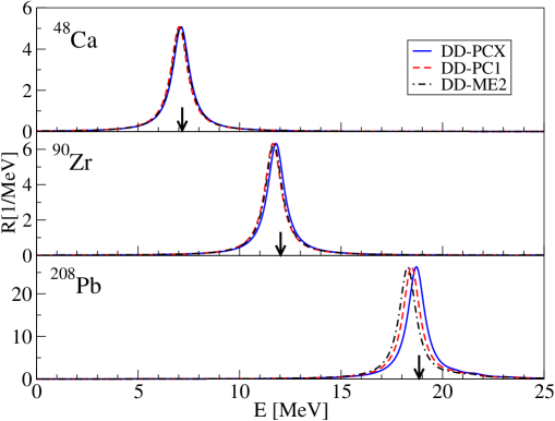
Figure 1: The PN-RRPA isobaric analog resonance transition strength distribution for ⁴⁸Ca, ⁹⁰Zr and ²⁰⁸Pb, calculated using DD-PCX, DD-PC1, and DD-ME2 functionals.

Next we explore the evolution of the IAR within the Sn isotope chain, for $A=$104$-$132. In Fig. 3 the IAR transition strength distributions are shown for representative cases, ^{112,116,122,130}Sn. Model calculations are based on the PN-RQRPA with DD-PCX interaction. The results without and with the $T=1$ proton-neutron pairing in the residual PN-RQRPA interaction are shown separately, in comparison to the experimental data from a systematic study of the (³He,t) charge-exchange reaction in stable Sn isotopes Pham et al. (1995). As shown in Fig. 3, the full PN-RQRPA calculations result in a pronounced single IAR peak, with the excitation energy that is in excellent agreement with the experimental data for ^112,116,122Sn Pham et al. (1995). Complete treatment of paring correlations both in the RHB and PN-RQRPA is essential for description of the IAR Paar et al. (2004). This is illustrated in Fig. 3, where the strength functions are also shown without including the $T=1$ proton-neutron residual pairing interaction, i.e., only the the $ph$-channel of the RQRPA residual interaction is included. Without the contributions of the $pp$-channel, pronounced fragmentation of the transition strength is obtained for ^112,116Sn, and the excitation energies are overestimated. By including the attractive proton-neutron pairing interaction, the transition strength becomes redistributed toward a single pronounced IAR peak, that is consistent with the expectation of a narrow resonance peak from the experimental study Pham et al. (1995). More pronounced effect of the residual pairing interaction is obtained for ^112,116,122Sn, while for ¹³⁰Sn that is near the neutron closed shell the effect is rather small.

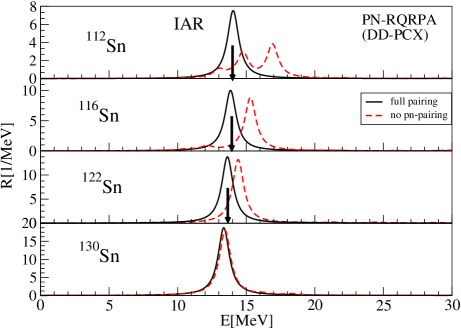
Figure 2: The isobaric analog resonance transition strength distribution for ^{112,116,122,130}Sn, calculated with the PN-RQRPA using DD-PCX interaction.The results without (dashed line) and with (solid line) proton-neutron pairing in the residual PN-RQRPA interaction are shown separately, in comparison to the experimental data from Ref. Pham et al. (1995), denoted by arrows.

Figure 3 shows the evolution of the IAR excitation energy for the isotopic chain ^104-132Sn, with the proton-neutron pairing included in the PN-RQRPA. The results are shown for the point coupling interactions DD-PCX and DD-PC1. For comparison, the IAR excitation energies from the previous study based on DD-ME1 interaction Paar et al. (2004) and the experimental data from Ref. Pham et al. (1995) are displayed. As one can observe in the figure, recently established interaction DD-PCX reproduces the experimental data with high accuracy, while the DD-PC1 and DD-ME1 interactions provide systematically lower energies. We note that DD-PCX parameterization has been established using additional constraints on nuclear collective transitions that resulted with improved isovector properties, essential for the description of nuclear ground state, excitation phenomena, and nuclear matter properties around the saturation density Yüksel et al. (2019). Clearly, the PN-RQRPA framework based on DD-PCX interaction introduced in this work represents a considerable progress in comparison to other approaches.

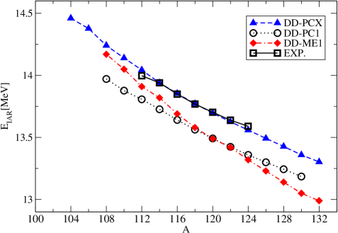
Figure 3: The PN-RQRPA isobaric analog resonance excitation energy for the isotope chain ^104-132Sn, with the proton-neutron pairing included. Calculations are based on the point coupling interaction DD-PCX and DD-PC1. The results from the previous study based on DD-ME1 interaction Paar et al. (2004) and the experimental data from Ref. Pham et al. (1995) are shown for comparison.

III.2 The Gamow-Teller resonance

The Gamow-Teller transitions involve both the spin and isospin degrees of freedom. In the charge-exchange excitation spectra, these transitions mainly concentrate in a pronounced resonance peak - Gamow-Teller resonance (GTR), representing a coherent superposition of $J^{\pi}=1^{+}$ proton-particle – neutron-hole transitions of neutrons from orbitals with $j=l+\frac{1}{2}$ into protons in orbitals with $j=l-\frac{1}{2}$. The GT transitions are excited by the spin-isospin operator

$$T_{\beta^{\pm}}^{GT}=\sum_{i=1}^{A}\bm{\Sigma}\tau_{\pm}\;.$$ (41)

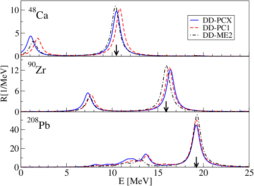
Figure 4: The GT^- strength distribution for ⁴⁸Ca, ⁹⁰Zr and ²⁰⁸Pb, calculated using the DD-PCX, DD-PC1, and DD-ME2 functionals. The experimental values of the main GT^- peak for ⁴⁸Ca Anderson et al. (1985a), ⁹⁰Zr Wakasa et al. (1997a) and ²⁰⁸Pb Akimune et al. (1995a); Pham et al. (1995); Horen et al. (1980) are denoted with arrows.

Figure 4 shows the GT^- transition strength distribution for closed shell nuclei ⁴⁸Ca, ⁹⁰Zr and ²⁰⁸Pb, calculated with the PN-RQRPA using DD-PCX and DD-PC1 interactions. For comparison, the results of the meson exchange functional with the DD-ME2 parameterization are also shown. The experimental values for the main GT^- peak are denoted with arrows for ⁴⁸Ca Anderson et al. (1985a), ⁹⁰Zr Bainum et al. (1980a); Wakasa et al. (1997a), and ²⁰⁸Pb Horen et al. (1980); Akimune et al. (1995a); Krasznahorkay et al. (2001a). Since the PN-RQRPA excitation energies are given with respect to the mother nucleus, the experimental values given with respect to daughter nucleus are modified by adding the mass difference between the daughter and mother isotopes as well as the mass difference between neutron and proton which is missing when the GT is built on the basis of p-h excitations Colò et al. (1994); Yüksel et al. (2020a). The transition strength distributions are dominated by the main Gamow-Teller resonance peak, that is composed from direct spin-flip transitions, ($j=l+\frac{1}{2}$ $\rightarrow$ $j=l-\frac{1}{2}$). In addition, pronounced low-energy GT^- strength is obtained, composed from the core-polarization spin-flip ($j=l\pm\frac{1}{2}$ $\rightarrow$ $j=l\pm\frac{1}{2}$), and back spin-flip transitions ($j=l-\frac{1}{2}$ $\rightarrow$ $j=l+\frac{1}{2}$). As it is well known, quantitative description of the low-energy GT^- strength is essential in modelling beta decay half-lives Marketin et al. (2007, 2016). When using three different effective interactions as shown in Fig. 4, the spread of values of the GT^- excitation energies within $\approx$ 1 MeV is obtained.

Table 1: Calculated and experimental GT^- properties, strength contributions for both GT^- and GT⁺ channel, i.e. $\sum B(\text{GT}^{-})$ and $\sum B(\text{GT}^{+})$, and total transition strengths $\sum B(\text{GT}^{-})-B(\text{GT}^{+})$ for ⁴⁸Ca, ⁹⁰Zr and ²⁰⁸Pb, for DD-PCX and DD-PC1 interactions. The total transition strengths are given in percentages of the Ikeda sum rule value $3(N-Z)$ Ikeda et al. (1963), and contributions from the negative energy states of the Dirac sea are shown. The experimental values for ⁴⁸Ca

are from Ref. Anderson et al. (1985a); Yako et al. (2009), ⁹⁰Zr from Refs. Bainum et al. (1980b); Wakasa et al. (1997b); Raywood et al. (1990); Condé et al. (1992), and ²⁰⁸Pb from Ref. Akimune et al. (1995b); Krasznahorkay et al. (2001b).

		48Ca	90Zr	208Pb
Experiment	$E_{1}$ ($E_{x}$) [MeV]	8.3 ($\approx 10.5$ Anderson et al. (1985a))	15.5	19.2
	FWHM1	1.5	3.8	4.1
	$E_{2}$ [MeV]	10.9	-	-
	FWHM2	3.9	-	-
	$\sum B(\text{GT}^{-}+\text{IVSM}^{-})$	$15.3\pm 2.2$ Yako et al. (2009)	$34.2\pm 1.6$ Wakasa et al. (1997b)	-
	$\sum B(\text{GT}^{-})$	-	$28.0\pm 1.6$Wakasa et al. (1997b)	-
	$\sum B(\text{GT}^{+}+\text{IVSM}^{+})$	$2.8\pm 0.3$ Yako et al. (2009)	-	-
	$\sum B(\text{GT}^{+})$	$1.9\pm 0.5$ Yako et al. (2009)	$1.0\pm 0.3$Raywood et al. (1990) ($1.7\pm 0.2$)Condé et al. (1992)	-
	$3(N-Z)$	24	30	132
	$\sum B(\text{GT}^{-})-B(\text{GT}^{+})$ [%]	$(52\pm 9)$% ($\approx 70\%$ Anderson et al. (1985a))	$(90\pm 5)\%$ Wakasa et al. (1997b)	$60-70\%$ Akimune et al. (1995b)
DD-PCX	$E_{x}$ [MeV]	10.61	16.73	19.21
	$\sum B(\text{GT}^{-})$	27.34	38.99	147.33
	$\sum B(\text{GT}^{+})$	3.34	8.89	15.33
	$\sum B(\text{GT}^{-})-B(\text{GT}^{+})$ [%]	99.96%	100.33%	99.99%
	Dirac sea [%]	6.48%	7.90%	8.23%
DD-PC1	$E_{x}$ [MeV]	10.98	16.54	19.21
	$\sum B(\text{GT}^{-})$	27.09	37.21	145.92
	$\sum B(\text{GT}^{+})$	3.10	7.05	13.93
	$\sum B(\text{GT}^{-})-B(\text{GT}^{+})$ [%]	99.97%	100.50%	99.99%
	Dirac sea [%]	5.93%	7.46%	7.48%

While the strength parameter of the pseudovector channel in the residual PN-R(Q)RPA interactions is constrained by the GTR excitation energy in ²⁰⁸Pb, reasonable agreement with experimental data is obtained for ⁴⁸Ca and ⁹⁰Zr without additional adjustments of the effective interaction. As it has already been discussed in previous studies, the Ikeda sum rule for GT transition strength Ikeda et al. (1963) is fully reproduced in a complete calculation that includes both the configurations formed from occupied states in the Fermi sea and empty negative-energy states in the Dirac sea  Kurasawa et al. (2003a, b); Ma et al. (2004); Kurasawa and Suzuki (2004); Paar et al. (2004). Table 1 shows the summary of the GTR properties for ⁴⁸Ca, ⁹⁰Zr and ²⁰⁸Pb for DD-PCX and DD-PC1 interactions: centroid excitation energies, the total transition strength difference $\sum B(\text{GT}^{-})-B(\text{GT}^{+})$ in comparison to the Ikeda sum rule Ikeda et al. (1963) (in $\%$), contributions of the Dirac sea states to the sum rule (in $\%$), and the respective experimental values Anderson et al. (1985b); Bainum et al. (1980b); Wakasa et al. (1997b); Akimune et al. (1995b); Yako et al. (2009). While the calculations accurately exhaust the Ikeda sum rule values, obtained total transition strengths in ⁴⁸Ca and ⁹⁰Zr for GT^- channel are somewhat larger than experimental ones for both point coupling interactions. After subtraction of the estimated IVSM contribution (usually $\sim 10\%$) the values of total GT^- strengths are even lower Yako et al. (2009). In the GT⁺ channel for ⁴⁸Ca the difference between theoretical and experimental values is reduced, i.e. $\sum B(\text{GT}^{+})=3.3$ ($3.0$) for DD-PCX (DD-PC1) and it is very close to the experimental value of $\sum B(\text{GT}^{+}+\text{IVSM}^{-})=2.8$ ($\sum B(\text{GT}^{+})=1.9$ without IVSM). However, the experimental strengths in ⁴⁸Ca may be significantly underestimated for higher excitation energies above 15 MeV in the GT^- spectrum and above 8 MeV in the GT⁺ spectrum Yako et al. (2009). The largest discrepancy in the GT⁺ channel is observed for ⁹⁰Zr, where calculated values are at least few times greater than the highest estimates of experimental GT⁺ strengthsCondé et al. (1992). Other nonrelativistic RPA approaches, such as Extended RPA theories account also somewhat larger value of $\sum B(\text{GT}^{-})$ (usually 10-20%) in lower part of ⁴⁸Ca excitation spectrum ($E_{x}\lesssim 20$ MeV)Rijsdijk et al. (1993). Both dressed and extended RPA theories overestimate total experimental strengths in ⁹⁰Zr for GT^- channel by $20-60\%$ for $E_{x}\lesssim 25$ MeV. However, in these calculations significant percentage of the sum rule for both GT^- and GT⁺ may be found for excitation energies above $E_{x}\gtrsim$ 40 MeV Rijsdijk et al. (1993), which is not the case in our calculations. The nonrelativistic QRPA + PVC calculations also overestimate the total experimental strengths in ⁴⁸Ca (71% of the RPA+PVC strength) and ²⁰⁸Pb (63% of the RPA+PVC strength) Niu et al. (2014), still not providing the explanation for the missing experimental strength. The contributions of the GT transitions to the empty Dirac sea in doubly magic nuclei is from $6.5-8.2\%$ ($5.9-7.5\%$) of the total strength for DD-PCX (DD-PC1), in agreement with the previous studies Paar et al. (2004).

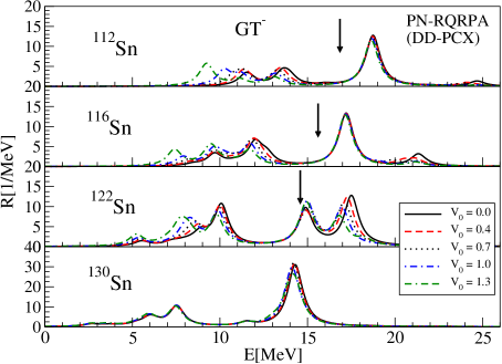
Figure 5: The GT^- strength distribution for ^{112,116,122,130}Sn, calculated with the PN-RQRPA using DD-PCX interaction, for the range of values of the isoscalar proton-neutron pairing interaction strength parameter, $V_{0}$=0-1.3. Experimental values for the main GT^- peaks for ¹¹²Sn, ¹¹⁶Sn and ¹²²Sn are denoted with arrows Pham et al. (1995).

In the following, the PN-RQRPA based on point coupling interaction DD-PCX is employed in the study of GT^- transitions in Sn istotope chain. For open shell nuclei, in addition to the separable pairing interaction included in the RHB, the PN-RQRPA residual interaction also includes the isoscalar proton-neutron pairing as introduced in Sec. II. Since this pairing interaction channel is not present within the RHB, its strength parameter $V_{0}$ can be constrained by the experimental data, e.g., on GT^- excitation energies or beta decay half-lives. Rather than providing the optimal value of $V_{0}$, in the present analysis we explore the pairing properties and sensitivity of the GT^- transitions by systematically varying $V_{0}$. In Fig.5, the GT^- strength distribution is shown for the isotopes ^{112,116,122,130}Sn, calculated with the PN-RQRPA using DD-PCX interaction. The isoscalar proton-neutron pairing interaction strength parameter is varied within the range of $V_{0}$=0-1.3 MeV. At higher excitation energies, a pronounced GT resonance peak is obtained, except for ¹²²Sn, where the main peak is split. In all cases, pronounced low-energy GT^- strength is obtained, spreading over the energy range of $\approx$ 5 MeV. While the direct spin-flip transitions ($\nu j=l+\frac{1}{2}$ $\rightarrow$ $\pi j=l-\frac{1}{2}$) dominate the high-energy region, the low-energy strength is dominated by core-polarization spin-flip ($\nu j=l\pm\frac{1}{2}$ $\rightarrow$ $\pi j=l\pm\frac{1}{2}$), and back spin-flip ($\nu j=l-\frac{1}{2}$ $\rightarrow$ $\pi j=l+\frac{1}{2}$) transitions. Considering the dependence of the GT^- strength on the $T=0$ proton-neutron pairing, one can observe in Fig.5 that the main GTR peak appears insensitive to this pairing interaction channel. In the low-energy region, pronounced sensitivity of the GT^- spectra on $V_{0}$ is obtained, i.e. with increased $V_{0}$ the strength is shifted toward lower energies. This result is in agreement with previous studies based on different effective interactions both in the $ph$ and $pp$ channels Paar et al. (2004).

Table 2: Calculated values of GTR properties for ¹¹²Sn, ¹¹⁶Sn, ¹²²Sn and ¹³⁰Sn with DD-PCX and DD-PC1 interactions and $T=0$ pairing strengths $V_{0}~{}=~{}0.7$ and $V_{0}~{}=~{}1.3$. The contributions of strengths in the GT^- and GT⁺ channels are shown in separate columns. The total strength of GTR is also represented in percentages of the Ikeda sum rule value, $3(N-Z)$ Ikeda et al. (1963). Contributions to total GTR strength from transitions to negative energy states of Dirac sea are also shown.

		$3(N-Z)$				Sum rule %
			$\sum B(\text{GT}^{-})$	$\sum B(\text{GT}^{+})$	$\sum\left(B(\text{GT}^{-})-B(\text{GT}^{+})\right)$	total	Dirac sea
DD-PCX	112Sn	36	47.22	11.68	35.53	98.69%	7.36%
$(V_{0}=0.7)$	116Sn	48	57.77	9.99	47.77	99.53%	7.84%
	122Sn	66	75.26	9.34	65.91	99.87%	7.87%
	130Sn	90	99.06	9.12	89.94	99.94%	7.76%
DD-PC1	112Sn	36	45.55	9.84	35.71	99.21%	7.11%
$(V_{0}=0.7)$	116Sn	48	57.03	9.26	47.77	99.53%	7.85%
	122Sn	66	74.41	8.47	65.94	99.91%	7.17%
	130Sn	90	98.23	8.26	89.96	99.96%	7.01%
DD-PCX	112Sn	36	45.68	10.15	35.52	98.69%	7.36%
$(V_{0}=1.3)$	116Sn	48	56.79	7.59	49.20	99.53%	7.85%
	122Sn	66	74.96	9.04	65.91	99.87%	7.87%
	130Sn	90	99.01	9.06	89.94	99.94%	7.76%
DD-PC1	112Sn	36	44.67	8.95	35.71	99.21%	7.12%
$(V_{0}=1.3)$	116Sn	48	56.29	8.46	47.82	99.64%	7.20%
	122Sn	66	74.26	8.32	65.94	99.91%	7.18%
	130Sn	90	98.20	8.23	89.96	99.96%	7.02%

In Tab. 2 the calculated GT strengths for the ^{112,116,122,130}Sn isotopes are shown for DD-PCX and DD-PC1 functionals, using $T~{}=~{}0$ strength parameter set to $V_{0}~{}=~{}0.7$ and $V_{0}~{}=~{}1.3$. The Ikeda sum rule Ikeda et al. (1963) is reasonably well reproduced.

In Tab. 3 calculated values of moments $m_{0}(\text{GT}^{-})$ are shown for the first three dominant GT^- peaks, with the corresponding excitation energies $m_{1}$/$m_{0}$ with respect to the IAS for ¹¹²Sn, ¹¹⁶Sn, ¹²²Sn and ¹³⁰Sn. Calculations include the DD-PCX functional and $T=0$ pairing strength $V_{0}~{}=~{}1.3$. We note that there are few methods one can use to constrain the value of parameter $V_{0}$. One of them is based on comparison of experimental and theoretical values of relative positions of the GT peaks with respect to the IAS. As shown in Fig. 5, the number, position and intensity of GT peaks strongly depend on the value of parameter $V_{0}$. In the GTR spectrum of Sn isotopes one can observe two less intensier distinguishable peaks for $V_{0}\lesssim 0.4$ in the lower part of spectrum (GT2 and (GT3), besides one (GT1) or two dominant peaks (GT1a and GT1b), which is characteristic for $A\gtrsim 122$. For values $V_{0}\gtrsim 0.4$ usually the third peak (GT4) starts to show up, while for values $V_{0}\gtrsim 0.7$ we have in general three smaller peaks in lower part of spectrum that may be distinguished. The position of these peaks and respective transition strengths are strongly influenced by $T~{}=~{}0$ pairing, i.e. with higher strength $V_{0}$ their positions move towards lower energies. Furthermore, the strength distribution is also modified, i.e. GT3 and GT4 peaks become more dominant than the GT2 ones for values $V_{0}\gtrsim 1.3$. The influence of $T~{}=~{}0$ pairing becomes suppressed when approaching the magic neutron number N=82, as observed in the GTR spectrum of ¹³⁰Sn. Experimental values of GT positions and cross sections obtained from Sn(³He,t)Sb reactions (see Ref. Pham et al. (1995)) have some hierarchy, with descending values of cross sections corresponding to each peak as the peak position is moved toward lower energies, with minor exception of GT4 which intensity is similar to the GT3 one or somewhat larger. Therefore we may impose some constraints on the value of $V_{0}$, which should be at least $\approx 0.7$ in order to reproduce the GTR properties observed in experiments.

Table 3: Calculated values of moments $m_{0}$ and corresponding energy $m_{1}/m_{0}$ with respect to the IAS for the first four dominant GT^- peaks for ¹¹²Sn, ¹¹⁶Sn, ¹²²Sn and ¹³⁰Sn. The DD-PCX functional and $T=0$ pairing strengths $V_{0}~{}=~{}0.7$ and $V_{0}~{}=~{}1.3$ are used. The experimental results for the difference between GTR and IAS, i.e. $\Delta^{\text{exp}}~{}=~{}E_{\text{GTR}}^{\text{exp}}-E_{\text{IAS}}^{\text{exp}}$ and differential cross sections ${d\sigma}/{d\Omega}$ are taken from Ref. Pham et al. (1995). ^†For ¹²²Sn, the moments $m_{0}$ and $m_{1}/m_{0}$ contain contributions from two most dominant peaks.

				——— $V_{0}~{}=~{}0.7$ ———			——— $V_{0}~{}=~{}1.3$ ———
		$\Delta^{\text{exp}}$	${d\sigma}/{d\Omega}$	$m_{0}$	$m_{1}/m_{0}$	$\left(\frac{m_{1}}{m_{0}}-E_{\text{IAS}}^{\text{teo}}\right)$	$m_{0}$	$m_{1}/m_{0}$	$\left(\frac{m_{1}}{m_{0}}-E_{\text{IAS}}^{\text{teo}}\right)$
		[MeV]	[mb/sr]		[MeV]	[MeV]		[MeV]	[MeV]
GT1	112Sn	2.78	12.4	19.11	18.70	4.85	17.69	18.63	4.78
	116Sn	1.68	16.8	20.51	17.19	3.45	19.71	17.15	3.41
	122Sn†	1.01	21.9	31.68	16.71	3.14	29.62	15.82	2.25
	130Sn	-	-	50.03	14.22	0.83	48.55	14.12	0.73
GT2	112Sn	-2.08	4.9	6.30	13.27	-0.58	3.69	13.05	-0.80
	116Sn	-3.32	6.2	10.02	11.85	-1.89	6.54	11.61	-2.13
	122Sn	-4.59	9.2	14.26	9.94	-3.63	11.27	9.78	-3.79
	130Sn	-	-	15.75	7.53	-5.86	16.07	7.40	-5.99
GT3	112Sn	-3.67	1.5	5.17	11.31	-2.54	2.54	11.06	-2.79
	116Sn	-5.18	2.1	3.04	10.64	-3.10	8.71	9.52	-4.22
	122Sn	-7.87	6.3	10.27	8.33	-5.24	12.81	7.87	-5.70
	130Sn	-	-	9.74	5.87	-7.52	10.90	5.80	-7.59
GT4	112Sn	-4.83	2.0	3.14	10.71	-3.14	8.94	9.01	-4.84
	116Sn	-6.52	2.5	2.05	8.12	-5.62	6.65	7.33	-6.41
	122Sn	-9.79	1.2	3.32	5.86	-7.71	5.64	5.59	-7.98

In Fig. 6 the PN-RQRPA results for the GT^- direct spin-flip transition excitation energy centroid with the respect to the IAR energy are shown for the chain of even-even isotopes ^104-132Sn. The available experimental data obtained from Sn(³He,t)Sb charge-exchange reactions are shown for comparison Pham et al. (1995). The PN-RQRPA calculations are performed for the range of values of the isoscalar proton-neutron pairing interaction strength parameter, $V_{0}$=0.4-2.5. The point coupling interaction DD-PCX is used and the results based on the DD-ME2 interaction are also displayed Paar et al. (2004). We noticed almost linear decrease of differences between the GTR and IAS energies in Sn isotope chain as function of A or N (while keeping $Z=50$ fixed). Similar observations may be found in nonrelativistic calculations with Skyrme parametrizations in Fracasso and Colò (2007). One can observe that the proton-neutron pairing interaction systematically reduces the GT-IAR energy splittings along the Sn isotope chain, resulting in good agreement for $V_{0}\approx$2.5. We note that relatively higher values of $V_{0}$ are required to reproduce the GT-IAR energy splittings. In Refs. Vretenar et al. (2003); Paar et al. (2004), it has been emphasized that the energy difference between the GTR and the IAS reflects the magnitude of the effective spin-orbit potential. As one can see in Fig. 6, the GT-IAR energy splittings reduce in neutron-rich Sn isotopes toward zero value, reflecting considerable reduction of the spin-orbit potential and the corresponding increase of the neutron skin thickness $r_{n}-r_{p}$ Vretenar et al. (2003). Therefore, as pointed out in Ref. Vretenar et al. (2003), the energy difference $E_{\rm GT}-E_{\rm IAS}$, obtained from the experiment, could be used to determine the value of neutron skin thickness in a consistent framework that can simultaneously describe the charge-exchange excitation properties and the $r_{n}-r_{p}$ value, such as the RHB+PN-RQRPA approach.

In Ref. Yüksel et al. (2020b) the GT^- transition strength for ¹¹⁸Sn was analyzed in more details, including the finite temperature effects, using the Skyrme functional SkM^∗. In the present study, for ¹¹⁸Sn without T=0 pairing and DD-PCX interaction ($V_{0}$=0), we obtain pronounced low-lying GT^- states at energies E=7.32, 8.88, 9.64, 10.21, and 11.45 MeV with the corresponding transition strengths B(GT^-)=1.21, 3.25, 1.12, 1.14, and 14.30. The main GTR peaks are obtained at E=16.46 and 19.83 MeV with B(GT^-)=19.91 and 7.69, respectively. The excitation energies are comparable with the respective values obtained for the SkM^∗ interaction in Ref. Yüksel et al. (2020b), E(GT^-)= 6.2, 8.9, 10.5, 16.3 and 20.2 MeV Yüksel et al. (2020b). Study in Ref. Yüksel et al. (2020b) also showed that relativistic calculations of GT^- transitions in ¹¹⁸Sn with density dependent meson-exchange interaction DD-ME2 lead to the splitting between major (GT1a) and energetically higher somewhat less intensive peak (GT1b), that exists only for $V_{0}\lesssim 200$ MeV in $T=0$ pairing channel. For $V_{0}\approx 200$ MeV the two peaks start to merge, while for $V_{0}\gtrsim 240$ MeV they are completely replaced by one somewhat stronger peak shifted $\approx 0.5$ MeV towards higher energies. However, nonrelativistic calculations in Refs. Yüksel et al. (2020b); Fracasso and Colò (2007) show different behavior in GT^- spectrum of ¹¹⁸Sn with respect to $T=0$ pairing strength, i.e. the two dominant peaks never merge, even for large values of overall strength of the $T=0$ pairing ($\approx 800$ MeV). The same feature is obtained in the present study, as shown in Fig. 5 for ¹²²Sn. We note that relativistic calculation in Ref. Yüksel et al. (2020b) used another pairing interaction in $T=0$ channel than the non-relativistic one, i.e. two Gaussians with different relative strengths to cover short and medium distances in coordinate space introduced separately for the PN-RQRPA. This caused additional interplay between attractive and repulsive terms which act differently for the short and medium ranges. Therefore, behavior of the GTR spectrum obtained in our study is more similar to the nonrelativistic calculations in Refs. Yüksel et al. (2020b); Fracasso and Colò (2007), where the zero range density dependent surface pairing in both isospin channels is introduced separately in the PN-RQRPA.

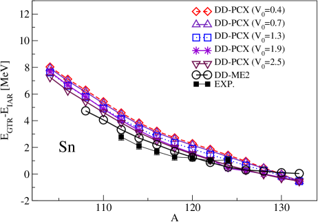
Figure 6: The PN-RQRPA excitation energy for GT^- direct spin-flip transitions for ^104-132Sn, for the range of values of the isoscalar proton-neutron pairing interaction strength parameter $V_{0}$. Calculations are based on the density dependent point coupling interaction DD-PCX and the results from the previous study based on the DD-ME2 interaction Paar et al. (2004) and the experimental data from Ref. Pham et al. (1995) are shown for comparison.

IV Conclusion

In this work we have formulated a consistent framework for description of nuclear charge-exchange transitions based on the proton-neutron relativistic quasiparticle random phase approximation in the canonical single-nucleon basis of the relativistic Hartree-Bogoliubov model, using density-dependent relativistic point coupling interactions. The implementation of recently established DD-PCX interactionYüksel et al. (2019), adjusted not only to the nuclear ground state properties, but also with the symmetry energy of the nuclear equation of state and the incompressibility of nuclear matter constrained using collective excitation data, allows improved description of ground-state and excitation properties of nuclei far from stability, that is important for the studies of exotic nuclear structure and dynamics, as well as for applications in nuclear astrophysics. The introduced formalism based on point coupling interactions is also relevant from the practical point of view, because it allows efficient systematic large-scale calculations of nuclear properties and processes of relevance for the nucleosynthesis and stellar evolution modeling. In the current formulation of the RHB+PN-RQRPA, the pairing correlations are implemented by the separable pairing force Tian et al. (2009) that allows accurate and efficient calculations of the pairing properties. The PN-RQRPA includes both the $T=1$ and $T=0$ pairing channels. While the $T=1$ channel corresponds to the pairing interaction constrained at the ground state level, $T=0$ proton-neutron pairing strength parameter can be determined from the experimental data on charge-exchange transitions and beta decay half lives. In order to validate the PN-R(Q)RPA framework introduced in this work, spin and isospin excitations - isobaric analog resonances and Gamow-Teller transitions - have been investigated in several closed-shell nuclei and Sn isotope chain. The results show very good agreement with the experimental data, representing an improvement compared to previous studies based on the relativistic nuclear energy density functionals. When compared to other theoretical approaches that usually underestimate the IAR excitation energies in Sn isotope chain, the present model using DD-PCX interaction accurately reproduces the experimental data. Therefore, the framework introduced in this work represents an important contribution for the future studies of astrophysically relevant nuclear excitations and weak interaction processes, in particular $\beta$-decay in neutron-rich nuclei, electron capture in presupernova stage of massive stars, and neutrino-nucleus reactions relevant for the synthesis of elements in the universe and stellar evolution. Especially important is the extension of theory framework introduced in this work to include both the finite temperature effects together with nuclear pairing and apply it for the description of electron capture and beta decay at finite temperature characteristic for stellar environment Yüksel et al. (2017, 2020a). This work is currently in progress Ravlić et al. (2020b, a).

Appendix A Particle-hole matrix elements

For the isovector-pseudovector part of particle-hole channel in the PN-RQRPA we use the contact type of interaction with constant coupling,

$$V_{PV}=-\alpha_{PV}[\gamma_{5}\ \gamma^{\nu}\vec{\tau}]_{1}\ [\gamma_{5}\gamma_{\nu}\vec{\tau}]_{2}\ \delta(\vec{r}_{1}-\vec{r}_{2}).$$ (42)

The uncoupled matrix element of isovector-pseudovector interaction is given by

$$\langle a\ b|V|c\ d\rangle~{}=~{}-\alpha_{PV}\int drr^{2}\sum_{L\lambda}\bigg{[}\int dr_{1}r_{1}^{2}\int d\Omega_{1}\bar{\psi}_{a}({r}_{1},\Omega_{1})[\gamma_{5}\ \gamma^{\nu}\vec{\tau}]_{(1)}Y_{L\lambda}^{*}(\Omega_{1})\\ ~{}\delta(r-r_{1})\psi_{c}({r}_{1},\Omega_{1})\bigg{]}\bigg{[}\int dr_{2}r_{2}^{2}\int d\Omega_{2}\bar{\psi}_{b}(r_{2},\Omega_{2})[\gamma_{5}\ \gamma_{\nu}\vec{\tau}]_{(2)}Y_{L\lambda}(\Omega_{2})\ \delta(r-r_{2})\ \psi_{d}({r}_{2},\Omega_{2})\bigg{]},$$ (43)

where we used expansion of delta function in spherical coordinates Ring and Schuck (2004),

$$\delta(\vec{r}_{1}-\vec{r}_{2})~{} =~{}\frac{\delta(r_{1}-r_{2})}{r_{1}r_{2}}\sum_{\lambda\mu}Y_{\lambda\mu}^{*}(\Omega_{1})Y_{\lambda\mu}(\Omega_{2})$$ (44)

$$=~{}\int drr^{2}\frac{\delta(r-r_{1})\delta(r-r_{2})}{r^{2}r_{1}r_{2}}\sum_{\lambda\mu}Y_{\lambda\mu}^{*}(\Omega_{1})Y_{\lambda\mu}(\Omega_{2}).$$ (45)

Indices $a$, $b$, $c$ and $d$ refer to all quantum numbers involved, while the Dirac’s conjugate is defined in standard way as

$$\bar{\psi}_{a}=\psi_{a}^{+}\ \gamma_{0}.$$ (46)

If we ignore for a moment the isospin part of the wave function (corresponding quantum numbers isospin $t$ and its third projection $t_{0}$) one can rewrite Eq. (43) in the following form:

$$\langle am_{a}\ bm_{b}|V|cm_{c}\ dm_{d}\rangle^{\text{PV}}~{}=-\alpha_{PV}\int drr^{2}\sum_{\lambda\mu}(-1)^{\mu}\sum_{\nu}\left[Q_{\lambda\mu}^{\nu}(r,\Omega_{1})\right]_{ac}\left[Q_{\lambda-\mu;\nu}(r,\Omega_{2})\right]_{bd}$$ (47)

where the index $\nu$ refers to Dirac matrix $\gamma_{\nu}$ ($\gamma^{\nu}$) in the vertex and we used (see Ref. Greiner and Bromley (2000) for the sherical case of spinor):

$$\left[Q_{\lambda\mu}^{\nu}(r,\Omega_{i})\right]_{am_{a}\ cm_{c}}~{}= ~{}\int d\Omega_{i}\left(f_{n_{a}\kappa_{a}}(r)\Omega_{\kappa_{a}m_{a}}^{\dagger}(\Omega_{i})~{}~{}-ig_{n_{a}\kappa_{a}}(r)\Omega_{\bar{\kappa}_{a}m_{a}}^{\dagger}(\Omega_{i})\right)[\gamma_{0}\gamma_{5}\ \gamma^{\nu}]_{(i)}$$

$$~{}\times Y_{\lambda\mu}(\Omega_{i})\left(\begin{array}[]{clcr}f_{n_{c}\kappa_{c}}(r)\Omega_{\kappa_{a}m_{c}}(\Omega_{i})\\ ig_{n_{c}\kappa_{c}}(r)\Omega_{\bar{\kappa}_{c}m_{c}}(\Omega_{i})\end{array}\right),$$ (50)

where the subscripts $1$ and $2$ refer to $\Omega_{\text{i = 1,2}}=\left(\theta_{i},\phi_{i}\right)$, while radial parts of bi-spinors $f(r)$ and $g(r)$ are assumed to be real in our case. From Eq. (50) one can easily obtain timelike

$$\left[Q_{\lambda\mu}^{0}(r,\Omega_{i})\right]_{am_{a}\ cm_{c}}~{}= ~{}-\bigg{[}i\ f_{n_{a}\kappa_{a}}(r)\ g_{n_{c}\kappa_{c}}(r){\langle(1/2\ l_{a})j_{a}m_{a}|\ Y_{\lambda\mu}(\Omega_{i})|(1/2\bar{l_{c}})j_{c}m_{c}\rangle}$$

$$-i\ g_{n_{a}\kappa_{a}}(r)\ f_{n_{c}\kappa_{c}}(r){\langle(1/2\bar{l_{a}})j_{a}m_{a}|\ Y_{\lambda\mu}(\Omega_{i})|(1/2l_{c})j_{c}m_{c}\rangle}\bigg{]}$$ (51)

and spacelike components ($k=1,2$ and $3$)

$$\left[Q_{\lambda\mu}^{k}(r,\Omega_{i})\right]_{am_{a}\ cm_{c}}~{}= ~{}-\bigg{[}f_{n_{a}\kappa_{a}}(r)f_{n_{c}\kappa_{c}}(r)\langle(1/2l_{a})j_{a}m_{a}|\sigma_{k}Y_{\lambda\mu}(\Omega_{1})|(1/2l_{c})j_{c}m_{c}\rangle$$

$$~{}+~{}g_{n_{a}\kappa_{a}}(r)g_{n_{c}\kappa_{c}}(r)\langle(1/2\bar{l}_{a})j_{a}m_{a}|\sigma_{k}Y_{\lambda\mu}(\Omega_{1})|(1/2\bar{l}_{c})j_{c}m_{c}\rangle\bigg{]}.$$ (52)

In order to couple particle and hole operator, i.e. states, into good total angular momentum J (and projection M) in the matrix elements of the residual particle-hole two body interaction, one needs to start from Suhonen (2007)

$$|(ph^{-1})JM\rangle~{} =~{}\left[c_{p}^{\dagger}h_{h}^{\dagger}\right]_{JM}|0\rangle$$ (53)

$$=~{}\sum_{m_{p}m_{h}}C_{j_{p}m_{p}j_{h}m_{h}}^{JM}c_{pm_{p}}^{\dagger}h_{hm_{h}}^{\dagger}|0\rangle$$ (54)

$$=\sum_{m_{p}m_{h}}(-1)^{j_{h}-m_{h}}C_{j_{p}m_{p}j_{h}-m_{h}}^{JM}a_{pm_{p}}^{\dagger}a_{h\ m_{h}}|0\rangle,$$ (55)

from which $JJ$-coupled particle-hole matrix element follows directly

$$\langle ac^{-1}|V|b^{-1}d\rangle^{JM}~{}= ~{}\sum_{m_{a}m_{c}}(-1)^{j_{c}-m_{c}}C_{j_{a}\ m_{a}\ jc\ -m_{c}}^{J\ M}\sum_{m_{b}m_{d}}(-1)^{j_{b}-m_{b}}C_{j_{d}\ m_{d}\ j_{b}\ -m_{b}}^{J\ M}$$

$$~{}~{}\langle am_{a}\ bm_{b}|V|cm_{c}\ dm_{d}\rangle.$$ (56)

Using the Wigner-Eckart theorem for angular parts in Eqs. (51) and (52) after some manipulations with Clebsch-Gordan coefficients one obtains the $ph$ matrix elements in $JJ$-coupled form. Therefore, after including isospin part of the matrix elements, which gives a factor of 2, which we have ignored for the moment, for the timelike part of pseudovector coupling we obtain:

$$V_{abcd}^{(PVt)J} =\frac{2\alpha_{PV}}{2J+1}\langle(1/2l_{a})j_{a}||Y_{J}(\Omega_{1})||(1/2\bar{l}_{c})j_{c}\rangle\langle(1/2{l}_{d})j_{d}||Y_{J}(\Omega_{2})||(1/2\bar{l}_{b})j_{b}\rangle$$

$$~{}~{}\int drr^{2}\bigg{[}f_{a}(r)g_{c}(r)-g_{a}(r)f_{c}(r)\bigg{]}\bigg{[}f_{b}(r)g_{d}(r)-g_{b}(r)f_{d}(r)\bigg{]}$$ (57)

and for spacelike part

$$V_{abcd}^{PV(s)J}~{}=~{}\frac{2\alpha_{PV}}{2J+1}\sum_{L}\int drr^{2}\bigg{[}f_{a}(r)f_{c}(r)\langle(1/2\ l_{a})j_{a}||\left[\sigma_{S}Y_{L}\right]_{J}||(1/2\ l_{c})j_{c}\rangle$$

$$~{}+~{}g_{a}(r)g_{c}(r)\langle(1/2\ \bar{l}_{a})j_{a}||\left[\sigma_{S}Y_{L}\right]_{J}||(1/2\ \bar{l}_{c})j_{c}\rangle\bigg{]}\bigg{[}f_{b}(r)f_{d}(r)\langle(1/2\ l_{d})j_{d}||\left[\sigma_{S}Y_{L}\right]_{J}||(1/2\ l_{b})j_{b}\rangle$$

$$~{}+~{}g_{b}(r)g_{d}(r)\langle(1/2\ \bar{l}_{d})j_{d}||\left[\sigma_{S}Y_{L}\right]_{J}||(1/2\ \bar{l}_{b})j_{b}\rangle\bigg{]},$$ (58)

where the reducible angular part of matrix elements can be written in terms of 3jm symbols:

$$\langle(1/2l_{a})j_{a}||Y_{J}||(1/2l_{c})j_{c}\rangle~{}=~{}\frac{1+(-1)^{l_{a}+l_{c}+J}}{2}\frac{\hat{j}_{a}\hat{j}_{c}\hat{J}}{\sqrt{4\pi}}(-1)^{j_{a}-1/2}\left(\begin{array}[]{clcr}j_{a}&J&j_{c}\\ -1/2&0&1/2\end{array}\right),$$ (59)

and

$$\langle(1/2l_{a})j_{a}||\left[\sigma_{S}Y_{L}\right]_{J}||(1/2l_{c})j_{c}\rangle~{}=~{}\frac{1+(-1)^{l_{a}+l_{c}+J}}{2}\frac{\hat{j}_{a}\hat{j}_{c}\hat{J}\hat{L}}{\sqrt{4\pi}}(-1)^{l_{a}+L}\Bigg{[}(-1)^{l_{c}+j_{c}+1/2}\\ ~{}\left(\begin{array}[]{clcr}1&L&J\\ 0&0&0\end{array}\right)\left(\begin{array}[]{clcr}j_{a}&J&j_{c}\\ -1/2&0&1/2\end{array}\right)-\sqrt{2}\left(\begin{array}[]{clcr}1&L&J\\ -1&0&1\end{array}\right)\left(\begin{array}[]{clcr}j_{a}&J&j_{c}\\ 1/2&-1&1/2\end{array}\right)\Bigg{]}.$$ (60)

Note that the timelike pseudovector matrix elements are non-zero only in the case of unnatural parity transitions, like Gamow-Teller transition. The isovector-vector part of two-body interaction is given by

$$V_{V}=\alpha_{V}\left[\rho_{V}(r_{1})\right][\gamma^{\mu}\vec{\tau}]_{1}\ [\gamma_{\mu}\vec{\tau}]_{2}\ \delta(\vec{r}_{1}-\vec{r}_{2}).\\$$ (61)

There are no additional rearrangement terms due to isospin restriction of the PN-R(Q)RPA, i.e. changing the nucleon from neutron to proton or vice versa and properties of the point coupling functional itself. Therefore, one should start from Eq. (61) and follow the same procedure described before, from Eqs. (43) to (58), replacing Eqs. (51) and (52) with

$$\left[Q^{k}_{\lambda\mu}(r,\Omega_{i})\right]_{am_{a}\ cm_{c}}~{}=~{}\bigg{[}if_{n_{a}\kappa_{a}}(r)g_{n_{c}\kappa_{c}}(r)\langle(1/2\ l_{a})j_{a}m_{a}|\sigma_{k}Y_{\lambda\mu}(\Omega_{i})|(1/2\ \bar{l}_{c})j_{c}m_{c}\rangle$$

$$-ig_{n_{a}\kappa_{a}}(r)f_{n_{c}\kappa_{c}}(r)\langle(1/2\ \bar{l}_{a})j_{a}m_{a}|\sigma_{k}Y_{\lambda\mu}(\Omega_{i})|(1/2l_{c})j_{c}m_{c}\rangle\bigg{]}$$ (62)

and

$$\left[Q^{0}_{\lambda\mu}(r,\Omega_{i})\right]_{am_{a}\ cm_{c}}~{}= ~{}\bigg{[}f_{n_{a}\kappa_{a}}(r)f_{n_{c}\kappa_{c}}(r)\langle(1/2\ l_{a})j_{a}m_{a}|Y_{\lambda\mu}(\Omega_{i})|(1/2\ {l}_{c})j_{c}m_{c}\rangle$$

$$~{}+~{}g_{n_{a}\kappa_{a}}(r)g_{n_{c}\kappa_{c}}(r)\langle(1/2\ \bar{l}_{a})j_{a}m_{a}|Y_{\lambda\mu}(\Omega_{i})|(1/2\ \bar{l}_{c})j_{c}m_{c}\rangle\bigg{]}$$ (63)

in order to obtain $JJ$-coupled $ph$ matrix elements for this channel, i.e. spacelike part

$$V_{abcd}^{(TVs)J}~{}=~{}\frac{2}{2J+1}\sum_{L}\int drr^{2}\alpha_{TV}\left[\rho_{V}(r)\right]\bigg{[}f_{a}(r)g_{c}(r)\langle(1/2\ l_{a})j_{a}||\left[\sigma_{S}Y_{L}\right]_{J}||(1/2\ \bar{l}_{c})j_{c}\rangle$$

$$~{}-g_{a}(r)f_{c}(r)\langle(1/2\ \bar{l}_{a})j_{a}||\left[\sigma_{S}Y_{L}\right]_{J}||(1/2\ l_{c})j_{c}\rangle\bigg{]}\bigg{[}f_{b}(r)g_{d}(r)\langle(1/2\ \bar{l}_{d})||\left[\sigma_{S}Y_{L}\right]_{J}||(1/2\ l_{b})j_{b}\rangle$$

$$~{}-g_{b}(r)f_{d}(r)\langle(1/2\ l_{d})j_{d}||\left[\sigma_{S}Y_{L}\right]_{J}||(1/2\ \bar{l}_{b})j_{b}\rangle\bigg{]}$$ (64)

and timelike part

$$V_{abcd}^{(TVt)J}~{}= ~{}\frac{2}{2J+1}\int drr^{2}\alpha_{TV}\left[\rho_{V}(r)\right]\bigg{[}f_{a}(r)f_{c}(r)+g_{a}(r)g_{c}(r))\bigg{]}\bigg{[}f_{b}(r)f_{d}(r)+g_{b}(r)g_{d}(r)\bigg{]}$$

$$~{}\times\langle(1/2\ l_{a})j_{a}||Y_{J}||(1/2\ l_{c})j_{c}\rangle\langle(1/2\ l_{d})j_{d}||Y_{J}||(1/2\ l_{b})j_{b}\rangle.$$ (65)

Appendix B Natural extension of separable pairing

In order to extend the standard $S~{}=~{}0$ ($T~{}=~{}1$) pairing, which was used in the RHB and RQRPA, one needs to start from general expression for particle-particle matrix element in the uncoupled form:

$$V_{abcd}~{}=~{}\langle n_{a}(1/2l_{a})j_{a}~{}n_{b}(1/2l_{b})j_{b}|V\left(1-\hat{P}^{r}\hat{P}^{\sigma}\hat{P}^{\tau}\right)|n_{c}(1/2l_{c})j_{c}~{}n_{d}(1/2l_{d})j_{d}\rangle$$ (66)

where $\hat{P}^{r}$, $\hat{P}^{\sigma}$ and $\hat{P}^{\tau}$ represent the exchange of relative spatial coordinate, spin and isospin, respectively. For action of the spin exchange operator $\hat{P}^{\sigma}$ we simply have

$$P^{\sigma}\left.|(1/2_{(1)}1/2_{(2)})SM_{S}\right\rangle~{}=~{}(-1)^{S+1}\left.|(1/2_{(1)}1/2_{(2)})SM_{S}\right\rangle,$$ (67)

which affects just the order of coupling, i.e. the phase $(-1)^{S+1}$ of symmetry transformation of the Clebsch-Gordan coefficient. Furthermore, one may construct $P^{\sigma}$ mathematically in the following way:

$$\hat{P}_{\sigma}~{}=~{}\frac{1+\vec{\sigma}_{1}\cdot\vec{\sigma}_{2}}{2},$$ (68)

and isospin exchange operator in analogous way. However, the action of $\hat{P}^{r}$ affects only relative spatial coordinates,

$$\hat{P}^{r}|\left.NLM_{L}\right\rangle~{}=~{}|\left.NLM_{L}\right\rangle,$$ (69)

$$\hat{P}^{r}|\left.nlm_{l}\right\rangle~{}=~{}(-1)^{l}|\left.nlm_{l}\right\rangle,$$ (70)

Therefore, as first step one needs to do the $LS$ recoupling in bra and ket independently

$$V_{abcd}^{\text{(pair)}J}~{}=~{}\hat{j}_{a}\hat{j}_{b}\hat{j}_{c}\hat{j}_{d}\sum_{\lambda S}\sum_{\lambda^{\prime}S^{\prime}}\hat{\lambda}\hat{S}\hat{\lambda^{\prime}}\hat{S^{\prime}}\left\{\begin{array}[]{clcr}s_{a}&l_{a}&j_{a}\\ s_{b}&l_{b}&j_{b}\\ S&\lambda&J\end{array}\right\}\left\{\begin{array}[]{clcr}s_{c}&l_{c}&j_{c}\\ s_{d}&l_{d}&j_{d}\\ S^{\prime}&\lambda^{\prime}&J\end{array}\right\}\sum_{TM_{T}}\sum_{T^{\prime}M_{T^{\prime}}}C_{1/2-1/21/21/2}^{TM_{T}}\\ C_{1/2-1/21/21/2}^{T^{\prime}M_{T^{\prime}}}\sum_{M_{S}M_{S}^{\prime}}C_{SM_{S}\lambda\mu}^{JM}C_{S^{\prime}M_{S}^{\prime}\lambda^{\prime}\mu^{\prime}}^{JM}\langle(1/2\ 1/2)TM_{T}|\langle(s_{a}s_{b})SM_{S}(l_{a}l_{b})\lambda\mu|V(1-\hat{P}^{r}\hat{P}^{\sigma}\hat{P}^{\tau})\\ |(s_{c}s_{d})S^{\prime}M_{S}^{\prime}(l_{c}l_{d})\lambda^{\prime}\mu^{\prime}\rangle|(1/2\ 1/2)T^{\prime}M_{T^{\prime}}\rangle.$$ (71)

In the second step one needs to substitute $V$ with generic separable form, similar to Eq. (17) but now without any kind of projection,

$$V(\vec{r}_{1},\vec{r}_{2},\vec{r}_{1}^{\prime},\vec{r}_{2}^{\prime})~{}=~{}-G_{0}\delta(\vec{R}_{1}-\vec{R}_{2})G(r)G(r^{\prime})$$ (72)

into Eq. (71) and transform the laboratory coordinates $\vec{r}_{1}$ and $\vec{r}_{2}$ ($\vec{r}_{1}^{\prime}$ and $\vec{r}_{2}^{\prime}$) in bra (ket) into the center of mass $\vec{R}$ ($\vec{R}^{\prime}$) and relative coordinates $\vec{r}$ ($\vec{r}^{\prime}$), i.e. the so-called Talmi-Moschinsky transformation. Therefore we need to evaluate

$$\sum_{TM_{T}}\sum_{T^{\prime}M_{T^{\prime}}} C_{1/2-1/21/21/2}^{TM_{T}}C_{1/2-1/21/21/2}^{T^{\prime}M_{T^{\prime}}}\langle(1/2\ 1/2)TM_{T}|\langle(1/2\ 1/2)SM_{S}(l_{a}l_{b})\lambda\mu|$$

$$V(1-\hat{P}^{r}\hat{P}^{\sigma}\hat{P}^{\tau})|(1/2\ 1/2)S^{\prime}M_{S^{\prime}}(l_{c}l_{d})\lambda^{\prime}\mu^{\prime}\rangle|(1/2\ 1/2)T^{\prime}M_{T^{\prime}}\rangle~{}=~{}$$

$$~{}= -4\pi G_{0}\delta_{SS^{\prime}}\delta_{M_{S}M_{S^{\prime}}}\delta_{\lambda L}\delta_{\mu m_{L}}\delta_{\lambda^{\prime}L}\delta_{\mu^{\prime}m_{L^{\prime}}}\sum_{NLnn^{\prime}}I_{n}I_{n^{\prime}}M_{n_{a}l_{a}n_{b}l_{b}}^{NLn0}M_{n_{c}l_{c}n_{d}l_{d}}^{NLn^{\prime}0}$$

$$\sum_{T}\frac{1}{2}\left(1+(-1)^{S^{\prime}+T+1}\right)$$ (73)

Constraining ourself to the proton-neutron case only, note that the only nonvanishing cases of the isospin coupling are $T=0$ and $M_{T}=0$ or $T=1$ and $M_{T}=0$, which both lead to factor $1/2$ in front of the round brackets in Eq. (71). Therefore, substituting back Eq. (73) into Eq. (71) after some mathematical manipulations we obtain

$$V_{abcd}^{JM}~{}= ~{}-G_{0}\hat{j}_{a}\hat{j}_{b}\hat{j}_{c}\hat{j}_{d}\sum_{LS}\sum_{T}\frac{1}{2}\left(1+(-1)^{S^{\prime}+T+1}\right)\tilde{f}(S,T)\hat{S}^{2}\hat{L}^{2}\left\{\begin{array}[]{clcr}l_{b}&1/2&j_{b}\\ l_{a}&1/2&j_{a}\\ L&S&J\end{array}\right\}\left\{\begin{array}[]{clcr}l_{d}&1/2&j_{d}\\ l_{c}&1/2&j_{c}\\ L&S&J\end{array}\right\}$$ (80)

$$~{}~{}~{}\sum_{nn^{\prime}}\tilde{I}_{n}\tilde{I}_{n}^{\prime}M_{n_{a}l_{a}n_{b}l_{b}}^{NLn0}M_{n_{c}l_{c}n_{d}l_{d}}^{NLn^{\prime}0}.$$ (81)

However, we also add multiplication with function $\tilde{f}(S,T)$ which should take into account somewhat smaller or enhanced effect of the pairing in $T~{}=~{}0$ case,

$$\tilde{f}(S,T)~{}=~{}\begin{cases}1,~{}{\text{for}~{}S=0~{},~{}T=1}\\ V_{0pp},~{}{\text{for}~{}S=1~{},~{}T=0}\\ 0,~{}{\text{the rest}}\end{cases}$$ (82)

while $\tilde{I}_{n}~{}=~{}\sqrt{4\pi}I_{n}$ is spatial integral of Gaussian $G(r)$ derived analytically in the next section of Appendix.

Appendix C Analytical solution of radial part

Radial part of the eigenfunction of spherical 3D harmonic oscillator is given by

$$R_{nl}(r,b_{0})~{}=~{}b_{0}^{-3/2}R_{nl}(\xi^{2})~{}=~{}b_{0}^{-3/2}N_{nl}\xi^{l}L_{n}^{l+1/2}(\xi^{2})e^{-\xi^{2}/2},$$ (83)

where $b_{0}$ represents oscillatory length, while $n$ corresponds to the nodes number (in this notation we don’t take into account 0 and $\infty$). Possible values are $n=0,1,2...$, and $\xi=r/b_{0}$. Normalization factor $N_{nl}$ is given by

$$N_{nl}~{}=~{}\left(\frac{2n!}{\Gamma(l+n+3/2)}\right)^{1/2}$$ (84)

In the case of half-number arguments gamma function is given by

$$\Gamma\left(\frac{1}{2}+n\right)~{}=~{}\frac{1\cdot 3\cdot 5\cdots(2n-1)}{2^{n}}\sqrt{\pi}~{}=~{}\frac{(2n-1)!!}{2^{n}}\sqrt{\pi},$$ (85)

We are interested in the analytical solution of the following integral

$$I_{n}~{}=~{}\int R_{nl}(r)G(r)r^{2}dr$$ (86)

By inserting G(r) from Eq. (18) in Eq. (86) we obtain

$$I_{n}~{}=~{}\frac{b_{0}^{3/2}N_{n0}}{(4\pi a^{2})^{3/2}}\int_{0}^{\infty}\exp\left[-\frac{\xi^{2}}{2}\left(\frac{b_{0}^{2}}{a^{2}}+1\right)\right]L_{n}^{1/2}(\xi^{2})\xi^{2}d\xi.$$ (87)

After substitution

$$\alpha^{2}~{}=~{}\frac{a^{2}}{b_{0}^{2}},~{}~{}\xi^{2}=\eta\rightarrow\xi d\xi=\frac{d\eta}{2},$$ (88)

Eq. (87) can be rewritten as

$$I_{n}~{}=~{}\frac{b_{0}^{-3/2}N_{n0}}{(4\pi\alpha^{2})^{3/2}}\frac{1}{2}\int_{0}^{\infty}\exp\left[-\eta+\frac{\eta}{2}\left(1-\frac{1}{\alpha^{2}}\right)\right]L_{n}^{(1/2)}(\eta)\sqrt{\eta}d\eta.$$ (89)

Generating function for Laguerre polynomials with $\alpha~{}=~{}1/2$ ($l~{}=~{}0$) is given by expression Abramowitz and Stegun (1965)

$$\frac{1}{(1-z)^{3/2}}\exp\left(\frac{xz}{z-1}\right)~{}=~{}\sum_{n=0}^{\infty}L_{n}^{1/2}(x)z^{n}.$$ (90)

By using substitution

$$\frac{1}{2}\left(1-\frac{1}{\alpha^{2}}\right)~{}=~{}\frac{z}{z-1}~{}\rightarrow~{}z~{}=~{}\frac{1-{\alpha^{2}}}{1+{\alpha^{2}}}$$ (91)

and Eq. (90), we can rewrite Eq. (89) in the following form,

$$I_{n}~{}=~{}\frac{b_{0}^{-3/2}N_{n0}}{(4\pi\alpha^{2})^{3/2}}\frac{1}{2}(1-z)^{3/2}\sum_{m=0}^{\infty}z^{m}\int_{0}^{\infty}d\eta\eta^{1/2}e^{-\eta}L_{n}^{(1/2)}(\eta)L_{m}^{(1/2)}(\eta).$$ (92)

The integral in Eq.(92) is just orthogonality condition for Laguerre’s polynomials Abramowitz and Stegun (1965),

$$\int_{0}^{\infty}x^{\alpha}e^{-\alpha}L_{n}^{\alpha}(x)L_{m}^{\alpha}(x)dx~{}=~{}\frac{\Gamma(n+\alpha+1)}{n!}\delta_{nm}.$$ (93)

Therefore, Eq. (92) reduces to

$$I_{n}~{}=~{}~{}\frac{1}{2}\frac{b_{0}^{-3/2}N_{n0}}{(4\pi\alpha^{2})^{3/2}}(1-z)^{3/2}\sum_{m=0}^{\infty}z^{m}\frac{\Gamma(m+3/2)}{m!}\delta_{nm}.$$ (94)

Using Eq. (85), inserting normalization factor (Eq. (84)) and expressing everything in terms of $\alpha$ and $n$, after some mathematical manipulations, it can further be simplified to

$$I_{n}~{}=~{}\frac{1}{2^{5/2}\pi^{5/4}b_{0}^{3/2}}\frac{(1-\alpha^{2})^{n}}{(1+\alpha^{2})^{n+3/2}}\frac{\sqrt{(2n+1)!}}{2^{n}n!}.$$ (95)

References

- Auerbach et al. (1972) N. Auerbach, J. Hüfner, A. K. Kerman, and C. M. Shakin, Rev. Mod. Phys. 44, 48 (1972).
- Auerbach (1983) N. Auerbach, Physics Reports 98, 273 (1983).
- Rumyantsev and Urin (1994) O. A. Rumyantsev and M. H. Urin, Phys. Rev. C 49, 537 (1994).
- Pham et al. (1995) K. Pham, J. Jänecke, D. A. Roberts, M. N. Harakeh, G. P. A. Berg, S. Chang, J. Liu, E. J. Stephenson, B. F. Davis, H. Akimune, and M. Fujiwara, Phys. Rev. C 51, 526 (1995).
- Colò et al. (1998) G. Colò, H. Sagawa, N. Van Giai, P. F. Bortignon, and T. Suzuki, Phys. Rev. C 57, 3049 (1998).
- Paar et al. (2004) N. Paar, T. Nikšić, D. Vretenar, and P. Ring, Phys. Rev. C 69, 054303 (2004).
- Fracasso and Colò (2005) S. Fracasso and G. Colò, Phys. Rev. C 72, 064310 (2005).
- Roca-Maza et al. (2012) X. Roca-Maza, G. Colò, and H. Sagawa, Phys. Rev. C 86, 031306 (2012).
- Roca-Maza and Paar (2018) X. Roca-Maza and N. Paar, Progress in Particle and Nuclear Physics 101, 96 (2018).
- Bender et al. (2002) M. Bender, J. Dobaczewski, J. Engel, and W. Nazarewicz, Phys. Rev. C 65, 054322 (2002).
- Marketin et al. (2012a) T. Marketin, G. Martínez-Pinedo, N. Paar, and D. Vretenar, Phys. Rev. C 85, 054313 (2012a).
- Litvinova et al. (2014) E. Litvinova, B. A. Brown, D. L. Fang, T. Marketin, and R. G. T. Zegers, Physics Letters B 730, 307 (2014).
- Ekström et al. (2014) A. Ekström, G. R. Jansen, K. A. Wendt, G. Hagen, T. Papenbrock, S. Bacca, B. Carlsson, and D. Gazit, Phys. Rev. Lett. 113, 262504 (2014).
- Zelevinsky et al. (2017) V. Zelevinsky, N. Auerbach, and B. M. Loc, Phys. Rev. C 96, 044319 (2017).
- Morita and Kanada-En’yo (2017) H. Morita and Y. Kanada-En’yo, Phys. Rev. C 96, 044318 (2017).
- Nabi et al. (2017) J.-U. Nabi, M. Ishfaq, M. Böyükata, and M. Riaz, Nuclear Physics A 966, 1 (2017).
- Ha and Cheoun (2017) E. Ha and M.-K. Cheoun, The European Physical Journal A 53, 26 (2017).
- Engel et al. (1988) J. Engel, P. Vogel, and M. R. Zirnbauer, Phys. Rev. C 37, 731 (1988).
- Borzov et al. (1995) I. Borzov, S. Fayans, and E. Trykov, Nuclear Physics A 584, 335 (1995).
- Engel et al. (1999) J. Engel, M. Bender, J. Dobaczewski, W. Nazarewicz, and R. Surman, Phys. Rev. C 60, 014302 (1999).
- Borzov (2003) I. N. Borzov, Phys. Rev. C 67, 025802 (2003).
- Madurga et al. (2016) M. Madurga, S. V. Paulauskas, R. Grzywacz, D. Miller, D. W. Bardayan, J. C. Batchelder, N. T. Brewer, J. A. Cizewski, A. Fijałkowska, C. J. Gross, M. E. Howard, S. V. Ilyushkin, B. Manning, M. Matoš, A. J. Mendez, K. Miernik, S. W. Padgett, W. A. Peters, B. C. Rasco, A. Ratkiewicz, K. P. Rykaczewski, D. W. Stracener, E. H. Wang, M. Woli ńska Cichocka, and E. F. Zganjar, Phys. Rev. Lett. 117, 092502 (2016).
- Marketin et al. (2016) T. Marketin, L. Huther, and G. Martínez-Pinedo, Phys. Rev. C 93, 025805 (2016).
- Moon et al. (2017) B. Moon, C.-B. Moon, A. Odahara, R. Lozeva, P.-A. Söderström, F. Browne, C. Yuan, A. Yagi, B. Hong, H. S. Jung, P. Lee, C. S. Lee, S. Nishimura, P. Doornenbal, G. Lorusso, T. Sumikama, H. Watanabe, I. Kojouharov, T. Isobe, H. Baba, H. Sakurai, R. Daido, Y. Fang, H. Nishibata, Z. Patel, S. Rice, L. Sinclair, J. Wu, Z. Y. Xu, R. Yokoyama, T. Kubo, N. Inabe, H. Suzuki, N. Fukuda, D. Kameda, H. Takeda, D. S. Ahn, Y. Shimizu, D. Murai, F. L. Bello Garrote, J. M. Daugas, F. Didierjean, E. Ideguchi, T. Ishigaki, S. Morimoto, M. Niikura, I. Nishizuka, T. Komatsubara, Y. K. Kwon, and K. Tshoo, Phys. Rev. C 96, 014325 (2017).
- Wang et al. (2016) Z. Y. Wang, Y. F. Niu, Z. M. Niu, and J. Y. Guo, Journal of Physics G: Nuclear and Particle Physics 43, 045108 (2016).
- Ravlić et al. (2020a) A. Ravlić, E. Yüksel, Y. F. Niu, and N. Paar, arXiv:2010.06394 [nucl-th] (2020a).
- Caballero-Folch et al. (2016) R. Caballero-Folch, C. Domingo-Pardo, J. Agramunt, A. Algora, F. Ameil, A. Arcones, Y. Ayyad, J. Benlliure, I. N. Borzov, M. Bowry, F. Calviño, D. Cano-Ott, G. Cortés, T. Davinson, I. Dillmann, A. Estrade, A. Evdokimov, T. Faestermann, F. Farinon, D. Galaviz, A. R. García, H. Geissel, W. Gelletly, R. Gernhäuser, M. B. Gómez-Hornillos, C. Guerrero, M. Heil, C. Hinke, R. Knöbel, I. Kojouharov, J. Kurcewicz, N. Kurz, Y. A. Litvinov, L. Maier, J. Marganiec, T. Marketin, M. Marta, T. Martínez, G. Martínez-Pinedo, F. Montes, I. Mukha, D. R. Napoli, C. Nociforo, C. Paradela, S. Pietri, Z. Podolyák, A. Prochazka, S. Rice, A. Riego, B. Rubio, H. Schaffner, C. Scheidenberger, K. Smith, E. Sokol, K. Steiger, B. Sun, J. L. Taín, M. Takechi, D. Testov, H. Weick, E. Wilson, J. S. Winfield, R. Wood, P. Woods, and A. Yeremin, Phys. Rev. Lett. 117, 012501 (2016).
- Faessler and Simkovic (1998) A. Faessler and F. Simkovic, Journal of Physics G: Nuclear and Particle Physics 24, 2139 (1998).
- Suhonen and Civitarese (1998) J. Suhonen and O. Civitarese, Physics Reports 300, 123 (1998).
- Šimkovic et al. (2011) F. Šimkovic, R. Hodák, A. Faessler, and P. Vogel, Phys. Rev. C 83, 015502 (2011).
- Menéndez et al. (2011) J. Menéndez, D. Gazit, and A. Schwenk, Phys. Rev. Lett. 107, 062501 (2011).
- Vergados et al. (2012) J. D. Vergados, H. Ejiri, and F. Šimkovic, Reports on Progress in Physics 75, 106301 (2012).
- Menéndez et al. (2014) J. Menéndez, T. R. Rodríguez, G. Martínez-Pinedo, and A. Poves, Phys. Rev. C 90, 024311 (2014).
- Štefánik et al. (2015) D. c. v. Štefánik, F. Šimkovic, and A. Faessler, Phys. Rev. C 91, 064311 (2015).
- Navas-Nicolás and Sarriguren (2015) D. Navas-Nicolás and P. Sarriguren, Phys. Rev. C 91, 024317 (2015).
- Delion and Suhonen (2017) D. S. Delion and J. Suhonen, Phys. Rev. C 95, 034330 (2017).
- Langanke and Martinez-Pinedo (2000) K. Langanke and G. Martinez-Pinedo, Nuclear Physics A 673, 481 (2000).
- Langanke and Martínez-Pinedo (2003) K. Langanke and G. Martínez-Pinedo, Rev. Mod. Phys. 75, 819 (2003).
- Janka et al. (2007) H. T. Janka, K. Langanke, A. Marek, G. Martínez-Pinedo, and B. Müller, The Hans Bethe Centennial Volume 1906-2006, Physics Reports 442, 38 (2007).
- Noji et al. (2014) S. Noji, R. G. T. Zegers, S. M. Austin, T. Baugher, D. Bazin, B. A. Brown, C. M. Campbell, A. L. Cole, H. J. Doster, A. Gade, C. J. Guess, S. Gupta, G. W. Hitt, C. Langer, S. Lipschutz, E. Lunderberg, R. Meharchand, Z. Meisel, G. Perdikakis, J. Pereira, F. Recchia, H. Schatz, M. Scott, S. R. Stroberg, C. Sullivan, L. Valdez, C. Walz, D. Weisshaar, S. J. Williams, and K. Wimmer, Phys. Rev. Lett. 112, 252501 (2014).
- Paar et al. (2015) N. Paar, T. Marketin, D. Vale, and D. Vretenar, International Journal of Modern Physics E 24, 1541004 (2015), http://www.worldscientific.com/doi/pdf/10.1142/S0218301315410049 .
- Niu et al. (2011) Y. F. Niu, N. Paar, D. Vretenar, and J. Meng, Phys. Rev. C 83, 045807 (2011).
- Niu et al. (2013) Z. M. Niu, Y. F. Niu, Q. Liu, H. Z. Liang, and J. Y. Guo, Phys. Rev. C 87, 051303 (2013).
- Ravlić et al. (2020b) A. Ravlić, E. Yüksel, Y. F. Niu, G. Coló, E. Khan, and N. Paar, arXiv:2006.08803 [nucl-th] (2020b).
- Arnould et al. (2007) M. Arnould, S. Goriely, and K. Takahashi, Physics Reports 450, 97 (2007).
- Mori et al. (2016) K. Mori, M. A. Famiano, T. Kajino, T. Suzuki, J. Hidaka, M. Honma, K. Iwamoto, K. Nomoto, and T. Otsuka, The Astrophysical Journal 833, 179 (2016).
- Ejiri (2000) H. Ejiri, Physics Reports 338, 265 (2000).
- Suzuki and Sagawa (2003) T. Suzuki and H. Sagawa, Nuclear Physics A 718, 446 (2003).
- Frekers et al. (2011) D. Frekers, H. Ejiri, H. Akimune, T. Adachi, B. Bilgier, B. A. Brown, B. T. Cleveland, H. Fujita, Y. Fujita, M. Fujiwara, E. Ganioğlu, V. N. Gavrin, E. W. Grewe, C. J. Guess, M. N. Harakeh, K. Hatanaka, R. Hodak, M. Holl, C. Iwamoto, N. T. Khai, H. C. Kozer, A. Lennarz, A. Okamoto, H. Okamura, P. P. Povinec, P. Puppe, F. Šimkovic, G. Susoy, T. Suzuki, A. Tamii, J. H. Thies, J. Van de Walle, and R. G. T. Zegers, Physics Letters B 706, 134 (2011).
- Cheoun et al. (2010) M.-K. Cheoun, E. Ha, S. Y. Lee, K. S. Kim, W. Y. So, and T. Kajino, Phys. Rev. C 81, 028501 (2010).
- Paar et al. (2008) N. Paar, D. Vretenar, T. Marketin, and P. Ring, Phys. Rev. C 77, 024608 (2008).
- Paar et al. (2011) N. Paar, T. Suzuki, M. Honma, T. Marketin, and D. Vretenar, Phys. Rev. C 84, 047305 (2011).
- Karakoç et al. (2014) M. Karakoç, R. G. T. Zegers, B. A. Brown, Y. Fujita, T. Adachi, I. Boztosun, H. Fujita, M. Csatlós, J. M. Deaven, C. J. Guess, J. Gulyás, K. Hatanaka, K. Hirota, D. Ishikawa, A. Krasznahorkay, H. Matsubara, R. Meharchand, F. Molina, H. Okamura, H. J. Ong, G. Perdikakis, C. Scholl, Y. Shimbara, G. Susoy, T. Suzuki, A. Tamii, J. H. Thies, and J. Zenihiro, Phys. Rev. C 89, 064313 (2014).
- Osterfeld (1992) F. Osterfeld, Rev. Mod. Phys. 64, 491 (1992).
- Fujita et al. (2011) Y. Fujita, B. Rubio, and W. Gelletly, Progress in Particle and Nuclear Physics 66, 549 (2011).
- Ikeda et al. (1963) K. Ikeda, S. Fujii, and J. I. Fujita, Physics Letters 3, 271 (1963).
- Doering et al. (1975) R. R. Doering, A. Galonsky, D. M. Patterson, and G. F. Bertsch, Phys. Rev. Lett. 35, 1691 (1975).
- Halbleib and Sorensen (1967) J. A. Halbleib and R. A. Sorensen, Nuclear Physics A 98, 542 (1967).
- Towner and Khanna (1979) I. S. Towner and F. C. Khanna, Phys. Rev. Lett. 42, 51 (1979).
- Goodman et al. (1980) C. D. Goodman, C. A. Goulding, M. B. Greenfield, J. Rapaport, D. E. Bainum, C. C. Foster, W. G. Love, and F. Petrovich, Phys. Rev. Lett. 44, 1755 (1980).
- Brown and Rho (1981) G. Brown and M. Rho, Nuclear Physics A 372, 397 (1981).
- Bertsch and Hamamoto (1982) G. F. Bertsch and I. Hamamoto, Phys. Rev. C 26, 1323 (1982).
- Nakayama et al. (1982) K. Nakayama, A. Pio Galeão, and F. Krmpotić, Physics Letters B 114, 217 (1982).
- Van Giai and Sagawa (1981) N. Van Giai and H. Sagawa, Physics Letters B 106, 379 (1981).
- Gaarde (1983) C. Gaarde, Nuclear Physics A 396, 127 (1983).
- Kuzmin and Soloviev (1984) V. A. Kuzmin and V. G. Soloviev, Journal of Physics G: Nuclear Physics 10, 1507 (1984).
- Colò et al. (1994) G. Colò, N. Van Giai, P. F. Bortignon, and R. A. Broglia, Phys. Rev. C 50, 1496 (1994).
- Hamamoto and Sagawa (1993) I. Hamamoto and H. Sagawa, Phys. Rev. C 48, R960 (1993).
- Brown and Rykaczewski (1994) B. A. Brown and K. Rykaczewski, Phys. Rev. C 50, R2270 (1994).
- Suzuki and Otsuka (1997) T. Suzuki and T. Otsuka, Phys. Rev. C 56, 847 (1997).
- De Conti et al. (1998) C. De Conti, A. Galeão, and F. Krmpotić, Physics Letters B 444, 14 (1998).
- Caurier et al. (1999) E. Caurier, K. Langanke, G. Martínez-Pinedo, and F. Nowacki, Nuclear Physics A 653, 439 (1999).
- Langanke et al. (2001) K. Langanke, E. Kolbe, and D. J. Dean, Phys. Rev. C 63, 032801 (2001).
- Algora et al. (2003) A. Algora, B. Rubio, D. Cano-Ott, J. L. Taín, A. Gadea, J. Agramunt, M. Gierlik, M. Karny, Z. Janas, A. Płochocki, K. Rykaczewski, J. Szerypo, R. Collatz, J. Gerl, M. Górska, H. Grawe, M. Hellström, Z. Hu, R. Kirchner, M. Rejmund, E. Roeckl, M. Shibata, L. Batist, and J. Blomqvist (GSI Euroball Collaboration), Phys. Rev. C 68, 034301 (2003).
- Kalmykov et al. (2006) Y. Kalmykov, T. Adachi, G. P. A. Berg, H. Fujita, K. Fujita, Y. Fujita, K. Hatanaka, J. Kamiya, K. Nakanishi, P. von Neumann-Cosel, V. Y. Ponomarev, A. Richter, N. Sakamoto, Y. Sakemi, A. Shevchenko, Y. Shimbara, Y. Shimizu, F. D. Smit, T. Wakasa, J. Wambach, and M. Yosoi, Phys. Rev. Lett. 96, 012502 (2006).
- Bai et al. (2009) C. L. Bai, H. Sagawa, H. Q. Zhang, X. Z. Zhang, G. Colò, and F. R. Xu, Physics Letters B 675, 28 (2009).
- Lutostansky (2011) Y. S. Lutostansky, Physics of Atomic Nuclei 74, 1176 (2011).
- Sasano et al. (2011) M. Sasano, G. Perdikakis, R. G. T. Zegers, S. M. Austin, D. Bazin, B. A. Brown, C. Caesar, A. L. Cole, J. M. Deaven, N. Ferrante, C. J. Guess, G. W. Hitt, R. Meharchand, F. Montes, J. Palardy, A. Prinke, L. A. Riley, H. Sakai, M. Scott, A. Stolz, L. Valdez, and K. Yako, Phys. Rev. Lett. 107, 202501 (2011).
- Niu et al. (2012) Y. F. Niu, G. Colò, M. Brenna, P. F. Bortignon, and J. Meng, Phys. Rev. C 85, 034314 (2012).
- Ha and Cheoun (2013) E. Ha and M.-K. Cheoun, Phys. Rev. C 88, 017603 (2013).
- Roca-Maza et al. (2013) X. Roca-Maza, G. Colò, and H. Sagawa, Physica Scripta 2013, 014011 (2013).
- Martini et al. (2014) M. Martini, S. Péru, and S. Goriely, Phys. Rev. C 89, 044306 (2014).
- Ha and Cheoun (2016) E. Ha and M.-K. Cheoun, Phys. Rev. C 94, 054320 (2016).
- Niu et al. (2016) Y. F. Niu, G. Colò, E. Vigezzi, C. L. Bai, and H. Sagawa, Phys. Rev. C 94, 064328 (2016).
- Liang et al. (2018) H. Z. Liang, H. Sagawa, M. Sasano, T. Suzuki, and M. Honma, Phys. Rev. C 98, 014311 (2018).
- Yasuda et al. (2018) J. Yasuda, M. Sasano, R. G. T. Zegers, H. Baba, D. Bazin, W. Chao, M. Dozono, N. Fukuda, N. Inabe, T. Isobe, G. Jhang, D. Kameda, M. Kaneko, K. Kisamori, M. Kobayashi, N. Kobayashi, T. Kobayashi, S. Koyama, Y. Kondo, A. J. Krasznahorkay, T. Kubo, Y. Kubota, M. Kurata-Nishimura, C. S. Lee, J. W. Lee, Y. Matsuda, E. Milman, S. Michimasa, T. Motobayashi, D. Muecher, T. Murakami, T. Nakamura, N. Nakatsuka, S. Ota, H. Otsu, V. Panin, W. Powell, S. Reichert, S. Sakaguchi, H. Sakai, M. Sako, H. Sato, Y. Shimizu, M. Shikata, S. Shimoura, L. Stuhl, T. Sumikama, H. Suzuki, S. Tangwancharoen, M. Takaki, H. Takeda, T. Tako, Y. Togano, H. Tokieda, J. Tsubota, T. Uesaka, T. Wakasa, K. Yako, K. Yoneda, and J. Zenihiro, Phys. Rev. Lett. 121, 132501 (2018).
- Liang et al. (2008) H. Liang, N. Van Giai, and J. Meng, Phys. Rev. Lett. 101, 122502 (2008).
- Niu et al. (2017) Z. M. Niu, Y. F. Niu, H. Z. Liang, W. H. Long, and J. Meng, Phys. Rev. C 95, 044301 (2017).
- Finelli et al. (2007) P. Finelli, N. Kaiser, D. Vretenar, and W. Weise, Nuclear Physics A 791, 57 (2007).
- Marketin et al. (2012b) T. Marketin, E. Litvinova, D. Vretenar, and P. Ring, Physics Letters B 706, 477 (2012b).
- Robin and Litvinova (2019) C. Robin and E. Litvinova, Phys. Rev. Lett. 123, 202501 (2019).
- Dechargé and Gogny (1980) J. Dechargé and D. Gogny, Phys. Rev. C 21, 1568 (1980).
- Berger et al. (1991) J. Berger, M. Girod, and D. Gogny, Computer Physics Communications 63, 365 (1991).
- Yüksel et al. (2019) E. Yüksel, T. Marketin, and N. Paar, Phys. Rev. C 99, 034318 (2019).
- Tian et al. (2009) Y. Tian, Z.-Y. Ma, and P. Ring, Phys. Rev. C 79, 064301 (2009).
- Nikšić et al. (2014) T. Nikšić, N. Paar, D. Vretenar, and P. Ring, Computer Physics Communications 185, 1808 (2014).
- Greiner and Bromley (2000) W. Greiner and D. Bromley, Relativistic Quantum Mechanics. Wave Equations (Springer, 2000).
- Horen et al. (1980) D. J. Horen, C. D. Goodman, C. C. Foster, C. A. Goulding, M. B. Greenfield, J. Rapaport, D. E. Bainum, E. Sugarbaker, T. G. Masterson, F. Petrovich, and W. G. Love, Physics Letters B 95, 27 (1980).
- Akimune et al. (1995a) H. Akimune, I. Daito, Y. Fujita, M. Fujiwara, M. B. Greenfield, M. N. Harakeh, T. Inomata, J. Jänecke, K. Katori, S. Nakayama, H. Sakai, Y. Sakemi, M. Tanaka, and M. Yosoi, Phys. Rev. C 52, 604 (1995a).
- Krasznahorkay et al. (2001a) A. Krasznahorkay, H. Akimune, M. Fujiwara, M. N. Harakeh, J. Jänecke, V. A. Rodin, M. H. Urin, and M. Yosoi, Phys. Rev. C 64, 067302 (2001a).
- Vretenar et al. (2005) D. Vretenar, A. Afanasjev, G. Lalazissis, and P. Ring, Physics Reports 409, 101 (2005).
- Buck and Merchant (1996) B. Buck and A. Merchant, Nuclear Physics A 600, 387 (1996).
- Kamuntavičius et al. (2001) G. Kamuntavičius, R. Kalinauskas, B. Barrett, S. Mickevičius, and D. Germanas, Nuclear Physics A 695, 191 (2001).
- Anderson et al. (1985a) B. D. Anderson, T. Chittrakarn, A. R. Baldwin, C. Lebo, R. Madey, P. C. Tandy, J. W. Watson, B. A. Brown, and C. C. Foster, Phys. Rev. C 31, 1161 (1985a).
- Bainum et al. (1980a) D. E. Bainum, J. Rapaport, C. D. Goodman, D. J. Horen, C. C. Foster, M. B. Greenfield, and C. A. Goulding, Phys. Rev. Lett. 44, 1751 (1980a).
- Wakasa et al. (1997a) T. Wakasa, H. Sakai, H. Okamura, H. Otsu, S. Fujita, S. Ishida, N. Sakamoto, T. Uesaka, Y. Satou, M. B. Greenfield, and K. Hatanaka, Phys. Rev. C 55, 2909 (1997a).
- Yüksel et al. (2020a) E. Yüksel, N. Paar, G. Colò, E. Khan, and Y. F. Niu, Phys. Rev. C 101, 044305 (2020a).
- Marketin et al. (2007) T. Marketin, D. Vretenar, and P. Ring, Phys. Rev. C 75, 024304 (2007).
- Yako et al. (2009) K. Yako, M. Sasano, K. Miki, H. Sakai, M. Dozono, D. Frekers, M. B. Greenfield, K. Hatanaka, E. Ihara, M. Kato, T. Kawabata, H. Kuboki, Y. Maeda, H. Matsubara, K. Muto, S. Noji, H. Okamura, T. H. Okabe, S. Sakaguchi, Y. Sakemi, Y. Sasamoto, K. Sekiguchi, Y. Shimizu, K. Suda, Y. Tameshige, A. Tamii, T. Uesaka, T. Wakasa, and H. Zheng, Phys. Rev. Lett. 103, 012503 (2009).
- Bainum et al. (1980b) D. E. Bainum, J. Rapaport, C. D. Goodman, D. J. Horen, C. C. Foster, M. B. Greenfield, and C. A. Goulding, Phys. Rev. Lett. 44, 1751 (1980b).
- Wakasa et al. (1997b) T. Wakasa, H. Sakai, H. Okamura, H. Otsu, S. Fujita, S. Ishida, N. Sakamoto, T. Uesaka, Y. Satou, M. B. Greenfield, and K. Hatanaka, Phys. Rev. C 55, 2909 (1997b).
- Raywood et al. (1990) K. J. Raywood, B. M. Spicer, S. Yen, S. A. Long, M. A. Moinester, R. Abegg, W. P. Alford, A. Celler, T. E. Drake, D. Frekers, P. E. Green, O. Häusser, R. L. Helmer, R. S. Henderson, K. H. Hicks, K. P. Jackson, R. G. Jeppesen, J. D. King, N. S. P. King, C. A. Miller, V. C. Officer, R. Schubank, G. G. Shute, M. Vetterli, J. Watson, and A. I. Yavin, Phys. Rev. C 41, 2836 (1990).
- Condé et al. (1992) H. Condé, N. Olsson, E. Ramström, T. Rönnqvist, R. Zorro, J. Blomgren, A. Håkansson, G. Tibell, O. Jonsson, L. Nilsson, P.-U. Renberg, M. Österlund, W. Unkelbach, J. Wambach, S. van der Werf, J. Ullmann, and S. Wender, Nuclear Physics A 545, 785 (1992).
- Akimune et al. (1995b) H. Akimune, I. Daito, Y. Fujita, M. Fujiwara, M. B. Greenfield, M. N. Harakeh, T. Inomata, J. Jänecke, K. Katori, S. Nakayama, H. Sakai, Y. Sakemi, M. Tanaka, and M. Yosoi, Phys. Rev. C 52, 604 (1995b).
- Krasznahorkay et al. (2001b) A. Krasznahorkay, H. Akimune, M. Fujiwara, M. N. Harakeh, J. Jänecke, V. A. Rodin, M. H. Urin, and M. Yosoi, Phys. Rev. C 64, 067302 (2001b).
- Kurasawa et al. (2003a) H. Kurasawa, T. Suzuki, and N. V. Giai, Phys. Rev. Lett. 91, 062501 (2003a).
- Kurasawa et al. (2003b) H. Kurasawa, T. Suzuki, and N. Van Giai, Phys. Rev. C 68, 064311 (2003b).
- Ma et al. (2004) Z. Ma, B. Chen, and N. e. a. Van Giai, Eur. Phys. J. A 20, 429 (2004).
- Kurasawa and Suzuki (2004) H. Kurasawa and T. Suzuki, Phys. Rev. C 69, 014306 (2004).
- Anderson et al. (1985b) B. D. Anderson, T. Chittrakarn, A. R. Baldwin, C. Lebo, R. Madey, P. C. Tandy, J. W. Watson, B. A. Brown, and C. C. Foster, Phys. Rev. C 31, 1161 (1985b).
- Rijsdijk et al. (1993) G. A. Rijsdijk, W. J. W. Geurts, M. G. E. Brand, K. Allaart, and W. H. Dickhoff, Phys. Rev. C 48, 1752 (1993).
- Niu et al. (2014) Y. F. Niu, G. Colò, and E. Vigezzi, Phys. Rev. C 90, 054328 (2014).
- Fracasso and Colò (2007) S. Fracasso and G. Colò, Phys. Rev. C 76, 044307 (2007).
- Vretenar et al. (2003) D. Vretenar, N. Paar, T. Nikšić, and P. Ring, Phys. Rev. Lett. 91, 262502 (2003).
- Yüksel et al. (2020b) E. Yüksel, N. Paar, G. Colò, E. Khan, and Y. F. Niu, Phys. Rev. C 101, 044305 (2020b).
- Yüksel et al. (2017) E. Yüksel, G. Colò, E. Khan, Y. F. Niu, and K. Bozkurt, Phys. Rev. C 96, 024303 (2017).
- Ring and Schuck (2004) P. Ring and P. Schuck, The Nuclear Many-Body Problem, Physics and astronomy online library (Berlin, Springer, 2004).
- Suhonen (2007) J. Suhonen, From Nucleons to Nucleus: Concepts of Microscopic Nuclear Theory, Theoretical and Mathematical Physics (Springer Berlin Heidelberg, 2007).
- Abramowitz and Stegun (1965) M. Abramowitz and I. Stegun, Handbook of Mathematical Functions: With Formulas, Graphs, and Mathematical Tables, Applied mathematics series (Dover Publications, 1965).