Momentum approach to the $1/r^{2}$ potential
as a toy model of the Wilsonian renormalization

Abstract

The Bessel operator, that is, the Schrödinger operator on the halfline with a potential proportional to $1/x^{2}$, is analyzed in the momentum representation. Many features of this analysis are parallel to the approach à la K. Wilson to Quantum Field Theory: one needs to impose a cutoff, add counterterms, study the renormalization group flow with its fixed points and limit cycles.

Keywords: Schrödinger operators, Bessel operators, momentum representation, renormalization group
MSC2020: 47E99, 81Q10, 81Q80

1 Introduction

Our paper is devoted to one of the most curious families of operators in mathematical physics,

$$L_{\alpha}\coloneqq-\frac{\mathrm{d}^{2}}{\mathrm{d}x^{2}}+\Big{(}\alpha-\frac{1}{4}\Big{)}\frac{1}{x^{2}},$$ (1.1)

where $\alpha\in\mathbb{R}$. $L_{\alpha}$ are often called Bessel operators. We will use the symbol $L_{\alpha}$ for the expression (1.1), without specifying its domain. Operators that are given by this expression and have a concrete domain will be called realizations of $L_{\alpha}$. Let us briefly list their most important properties.

Bessel operators are Hermitian (symmetric) on $C_{\mathrm{c}}^{\infty}(\mathbb{R}_{+})$. However, they are essentially self-adjoint only for $\alpha\geq 1$. For $\alpha<1$ they possess a 1-parameter family of self-adjoint realizations. In the terminology of Weyl, [25], $0$ is limit point for $\alpha>1$ and limit circle for $\alpha\leq 1$.

For $\alpha\neq 0$ their self-adjoint realizations can be described by specifying boundary conditions at zero as appropriate mixtures of $x^{\frac{1}{2}+m}$ and $x^{\frac{1}{2}-m}$, where $m:=\sqrt{\alpha}$. For $\alpha=0$, one needs to take mixtures of $x^{\frac{1}{2}}$ and $x^{\frac{1}{2}}\ln x$ and there is a curious “phase transition”: $m$ is real for $\alpha\geq 0$ and imaginary for $\alpha<0$. Moreover, all self-adjoint realizations of $L_{\alpha}$ are bounded from below for $\alpha\geq 0$ and unbounded from below for $\alpha<0$.

Many quantities related to $L_{\alpha}$ can be computed explicitly. For instance, the eigenfunction expansion of $L_{\alpha}$ can be given in terms of Bessel functions, see e.g. the classic book by Titchmarsh [23]. This allows us to describe explicitly all self-adjoint realizations of $L_{\alpha}$, as discussed by many authors, e.g. [19, 1, 6, 20, 17, 10, 5, 11, 8, 4, 16].

It is useful to note that $d$-dimensional Schrödinger operators with the inverse square potential

$$L_{\alpha,d}:=-\Delta_{d}+\frac{g}{r^{2}}$$ (1.2)

can be reduced to $1$-dimensional ones (1.1). In fact, if we restrict (1.2) to spherical harmonics of degree $l$ and make a simple transformation, then the radial operator coincides with $L_{\alpha}$, where

$${\alpha=\Big{(}\frac{d}{2}-1+l\Big{)}^{2}.}$$ (1.3)

In our paper, for simplicity we always stick to the dimension $1$, except for a short resume of the reduction of the $3$- to the $1$-dimensional case.

One of the most striking properties of Bessel operators is their homogeneity of degree $-2$. In other words, if $U_{\tau}$ denotes the scaling transformation (see (2.11)), then

$$U_{\tau}L_{\alpha}U_{\tau}^{-1}=\mathrm{e}^{-2\tau}L_{\alpha}.$$ (1.4)

This suggests us to introduce the transformation

$$R_{\tau}(B):=\mathrm{e}^{2\tau}U_{\tau}BU_{\tau}^{-1},$$ (1.5)

acting on, say, self-adjoint operators. $\mathbb{R}\ni\tau\mapsto R_{\tau}$ is a representation of the group $\mathbb{R}$ and preserves the set of self-adjoint realizations of $L_{\alpha}$. Some of these realizations are “fixed points” of $R_{\tau}$. There is an interesting analogy between the action of $R_{\tau}$ (1.5) on self-adjoint extensions of Bessel operators and the renormalization group acting on models of Quantum Field Theory (QFT).

The most obvious approach to Bessel operators is to study them in the position representation, as it is usually done in the literature. Our paper is devoted to an analysis of Bessel operators in the momentum representation. We believe that this is interesting in itself—in fact, many things look very different on the momentum side. Our main motivation, however, comes from the physics literature, where some authors try to explain the renormalization group approach to QFT by using Bessel operators as a toy model.

In QFT one can work both in the position and in the momentum space. The position representation is used in the so-called Epstein-Glaser approach. In practice, however, physicists prefer to work in the momentum representation, which is usually more convenient for computations. In order to compute various useful quantities one typically needs to impose a cutoff at momentum $\Lambda$ and to add appropriate $\Lambda$-dependent counterterms. The desired quantities are obtained in the limit $\Lambda\to\infty$, provided that various parameters are appropriately adjusted.

This procedure was greatly clarified by the Nobel prize winner K. Wilson, who stressed the role of scaling transformations in the process of renormalization. He also pointed out that it is not so important whether QFT has a well defined limit for $\Lambda\to\infty$: what matters is a weak dependence of low energy quantities on the high energy cutoff.

A number of authors [7, 2, 18, 15, 3], mostly with a high energy physics background, noticed that Bessel operators have a great pedagogical potential to illustrate the concept of renormalization group and Wilson’s ideas. In particular we would like to draw the reader’s attention to a recent paper [7], which is the main inspiration for our work. Reference [7] looks at the operator (1.2) in dimension 3 in the momentum representation. Its naive formulation is ill-defined due to diverging integrals at large momenta and does not select a self-adjoint realization. To cure these problems [7] applies the following steps, parallel to the usual approach to QFT:

Cut off the formal Hamiltonian with a momentum cutoff $$|p|<\Lambda$$. (1.6a)

Add an appropriate countertem multiplied by a running coupling constant. (1.6b)

Determine the differential equation for the coupling constant. (1.6c)

Take the limit $$\Lambda\to\infty$$. (1.6d)

The exposition contained in [7] stays all the time on the momentum side, and the reader may find it difficult to connect it to the standard theory of self-adjoint realizations of Bessel operators, more transparent in the position representation.

After describing the main source of motivation of our paper, let us outline its content. We start with Sec. 2 containing a brief resumé of the theory of self-adjoint realizations of Bessel operators in the position representation. We follow the terminology and conventions of [8, 4].

In Sec. 3 we recapitulate the content of [7]. On purpose, we stick to the original terminology and line of reasoning. In particular, we use the 3-dimensional setting, which can clearly be reduced to 1 dimension by the use of spherical coordinates.

Sec. 4 is the main part of our work. We start with a brief analysis of the momentum approach to general Schrödinger operators. We are mostly interested in operators on the half-line $\mathbb{R}_{+}$, and not on the whole line $\mathbb{R}$. This is consistent with the many-dimensional analysis in spherical coordinates, where the radius is always positive. We encounter the following issue: the usual Fourier transformation is adapted to the line, whereas on the half-line we have two natural cousins of the Fourier transformation: the sine and the cosine transformation (see (4.6), resp. (4.7)). The former diagonalizes the Dirichlet Laplacian $-\Delta_{\mathrm{D}}$, and the latter the Neumann Laplacian $-\Delta_{\mathrm{N}}$. Which approach we should choose? One can argue that from the 1-dimensional point of view both are equally natural. Therefore, we discuss both approaches. Actually, from the 3-dimensional point of view the sine transformation should be preferred, because the 3-dimensional Laplacian in the s-wave sector reduces to the Dirichlet Laplacian on the half-line.

Let us briefly describe the momentum approach to Schrödinger operators on $\mathbb{R}_{+}$ for sufficiently nice potentials. There are two basic Schrödinger operators with the potential $V$ on the halfline: $-\Delta_{\mathrm{D}}+V(x)$ and $-\Delta_{\mathrm{N}}+V(x)$. By applying the sine transformation to the former and the cosine transformation to the latter we obtain the operators

$$\tilde{H}_{\mathrm{D}}\psi(p)=p^{2}\psi(p)+\frac{1}{2\pi}\int_{0}^{\infty}(\tilde{V}(p-q)-\tilde{V}(p+q)\big{)}\psi(q)\mathrm{d}q,$$ (1.7)

$$\tilde{H}_{\mathrm{N}}\psi(p)=p^{2}\psi(p)+\frac{1}{2\pi}\int_{0}^{\infty}(\tilde{V}(p-q)+\tilde{V}(p+q)\big{)}\psi(q)\mathrm{d}q.$$ (1.8)

Here, $\tilde{V}(p)$ is the Fourier transform of the even extension of $V$ from $\mathbb{R}_{+}$ to $\mathbb{R}$.

If the potential is singular at $0$, say, non-integrable, we have several problems:

1. We cannot use the standard Dirichlet/Neumann boundary conditions.

2. We need to interpret $V$ as an irregular distribution.

3. The Fourier transform of $V$ will grow at infinity, making the formulas (1.7) and (1.8) problematic.

All these problems are present for Bessel operators, where $V$ is proportional to $\frac{1}{x^{2}}$. In particular, $\frac{1}{x^{2}}$ does not define a regular distribution. There exists, however, a well-known one-parameter family of even distributions that outside of $0$ coincide with $\frac{1}{x^{2}}$. Their Fourier transforms are

$$-\pi|p|+a,$$ (1.9)

where $a$ is a constant.

A priori it is not obvious which transformation is more appropriate for Bessel operators: the sine or the cosine transformation. Let us consider both, setting

$$\tilde{L}_{\alpha,\mathrm{D}} :=\mathcal{F}_{\mathrm{D}}L_{\alpha}\mathcal{F}_{\mathrm{D}},$$ (1.10)

$$\tilde{L}_{\alpha,\mathrm{N}} :=\mathcal{F}_{\mathrm{N}}L_{\alpha}\mathcal{F}_{\mathrm{N}},$$ (1.11)

where $L_{\alpha}$ is treated as a formal expression, $\cal{F}_{\mathrm{D}/\mathrm{N}}$ is the sine/cosine transformation.

Let us use $-\pi|p|$ as the Fourier transform of $\frac{1}{x^{2}}$. (We set $a=0$ in (1.9). This constant will reappear in disguise of a counter-term anyway later.) (1.7) and (1.8) yield formal expressions

$$\tilde{L}_{\alpha,\mathrm{D}}\psi(p) =p^{2}\psi(p)+\Big{(}\alpha-\frac{1}{4}\Big{)}\int_{0}^{\infty}\big{(}\theta(p-q)q+\theta(q-p)p\big{)}\psi(q)\mathrm{d}q,$$ (1.12)

$$\tilde{L}_{\alpha,\mathrm{N}}\psi(p) =p^{2}\psi(p)-\Big{(}\alpha-\frac{1}{4}\Big{)}\int_{0}^{\infty}\big{(}\theta(p-q)p+\theta(q-p)q\big{)}\psi(q)\mathrm{d}q,$$ (1.13)

where $\theta$ is the Heaviside function. Both expressions are problematic for large momenta. In what follows we give two constructions of self-adjoint realizations of (1.12) and (1.13). The first construction will be called “mathematicians’ style”, and the second “physicists’ style”.

The construction in “mathematicians’ style” directly describes the domains and actions of the operators. It starts with a construction of the minimal Bessel operators, denoted $\tilde{L}_{\alpha,\mathrm{D}}^{\min}$ and $\tilde{L}_{\alpha,\mathrm{N}}^{\min}$. They are defined by (1.12) and (1.13) on appropriate domains consisting of rapidly decaying functions. In addition, for (1.12) we need to assume that $\int_{0}^{\infty}\psi(p)p\mathrm{d}p=0$ and for (1.13) $\int_{0}^{\infty}\psi(p)\mathrm{d}p=0$.

The adjoints of the minimal Bessel operators are called the maximal Bessel operators, and denoted $\tilde{L}_{\alpha,\mathrm{D}}^{\max}$ and $\tilde{L}_{\alpha,\mathrm{N}}^{\max}$. If $\alpha\geq 1$, they coincide with the minimal Bessel operators, and also with their unique self-adjoint realizations. This is not the case for $\alpha<1$. The construction of maximal operators in the momentum representation is somewhat tricky. To obtain the maximal domains, $\mathcal{D}(\tilde{L}_{\alpha,\mathrm{D}}^{\min})$ and $\mathcal{D}(\tilde{L}_{\alpha,\mathrm{N}}^{\min})$ have to be extended by adjoining appropriate 2-dimensional subspaces. We cannot directly use the expressions (1.12) and (1.13), since now they usually contain divergent integrals. If $\alpha\neq\frac{1}{4}$ (that is, when there is a non-trivial potential), this additional subspace is spanned by certain vectors that behave for large $p$ as $p^{-\frac{3}{2}+m}$ and $p^{-\frac{3}{2}-m}$. Curiously, the case $\alpha=\frac{1}{4}$ is more problematic and has to be treated separately.

Finally, we define self-adjoint realizations of Bessel operators by selecting appropriate domains larger than the minimal but smaller than the maximal domain.

The above construction of self-adjoint Bessel operators is mathematically correct, but it sounds rather artificial. In the remaining part of Sect. 4 we describe “physicists’ style” construction, directly inspired by [7] and by the literature on QFT in general. This construction involves the four steps indicated in (1.6). Let us describe them more precisely.

The counterterms will be constructed out of (unbounded and non-closable) operators $K_{\mathrm{D}}$ and $K_{\mathrm{N}}$:

$$K_{\mathrm{D}}\psi(p) :=p\int_{0}^{\infty}q\psi(q)\mathrm{d}q,$$ (1.14)

$$K_{\mathrm{N}}\psi(p) :=\int_{0}^{\infty}\psi(q)\mathrm{d}q,$$ (1.15)

Suppose that $f_{\Lambda}$ and $g_{\Lambda}$ are solutions of the differential equations

$$\Lambda\frac{\mathrm{d}}{\mathrm{d}\Lambda}f_{\Lambda} =\Big{(}f_{\Lambda}+\frac{1}{4}+\alpha\Big{)}^{2}-\alpha,$$ (1.16)

$$\Lambda\frac{\mathrm{d}}{\mathrm{d}\Lambda}g_{\Lambda} =-\Big{(}g_{\Lambda}{+}\frac{1}{4}{+}\alpha\Big{)}^{2}+\alpha.$$ (1.17)

Let $p$ denote the momentum operator. Consider the operators

$$\theta(\Lambda-p)\Big{(}\tilde{L}_{\alpha,\mathrm{D}}+\frac{f_{\Lambda}}{\Lambda}K_{\mathrm{D}}\Big{)}\theta(\Lambda-p),$$ (1.18)

$$\theta(\Lambda-p)\Big{(}\tilde{L}_{\alpha,\mathrm{N}}+\Lambda g_{\Lambda}K_{\mathrm{N}}\Big{)}\theta(\Lambda-p).$$ (1.19)

Note that (1.18) and (1.19) are well-defined bounded self-adjoint operators. We prove that for $\alpha<1$ they converge then in the strong resolvent sense to self-adjoint realizations of the Bessel operator in the momentum representation. This can be viewed as the main result of our paper.

According to “physicists’ style construction” self-adjoint realizations of Bessel operators are parametrized by real solutions to the equations (1.16) and (1.17). Not surprisingly, these equations look very similar to various equations for running coupling constants used in QFT. Note also that the right hand sides of (1.16) and (1.17) depend analytically on $\alpha$ also at the “phase transition” $\alpha=0$. This phase transition is visible when we consider real solutions to these equations.

What is the take-home message of our paper? We do not insist that Schrödinger operators should be always studied in the momentum representation. However, we think that it is useful to know how the world looks “on the momentum side of the Fourier transform”. And it does look quite differently from the position representation.

To our knowledge, mathematicians rarely use the momentum representation to study Schrödinger operators. In particular, we have never seen the formulas (1.7) and (1.8) in mathematics papers. In physics papers, the momentum representation seems to be more common. For instance, the formula (1.7) can be found in [7] (in the 3-dimensional context).

The original purpose of our paper was to present the ideas of [7] in clear and rigorous terms. We think that these ideas are important and instructive. One can try to formulate them as follows. In renormalizable Quantum Field Theories most terms in the Lagrangian have the same homogeneity wrt the scaling. E.g in the Standard Model only the Higgs mass term has a different scaling dimension. Bessel operators are also almost homogeneous, with scaling invariance broken only by the boundary condition at $0$. This homogeneity is related to the fact that the naive formulations of both QFT and Bessel operators in the momentum representation are highly singular. Computations in QFT usually involve the four steps described in (1.6): imposing a momentum cutoff $\Lambda$, adding counterterms, solving the differential equation for the coupling constant and taking the limit $\Lambda\to\infty$. Our paper shows that the same steps have to be followed in a much simpler context of Bessel operators. These steps are not restricted to the difficult and complicated formalism of QFT. They are typical of the momentum approach.

Equations (1.16) and (1.17) have a one-parameter family of solutions for any $\alpha\in\mathbb{R}$. However, Bessel operators have a one-parameter family of self-adjoint realizations only for $\alpha<1$. In the language of QFT, “nontrivial renormalized theories” exist only for $\alpha<1$. For $\alpha\geq 1$ the ”flows of operators” (1.18) and (1.19) do not have limits in the sense of the Hilbert space $L^{2}(\mathbb{R}_{+})$, apart from the unique self-adjoint realizalion of $L_{\alpha}$. Hence for $\alpha\geq 1$, as Wilson suggested, “one can never remove the cutoff completely in a nontrivial theory”.

In particular, this is the case for the borderline value $\alpha=1$. The Bessel operator $L_{1}$ is the radial part of the Laplacian in 4 dimensions, see (1.3). We believe that it is not a coincidence that our spacetime also has 4 dimensions.

2 Position approach

2.1 Extensions of Hermitian operators

Let us recall basic concepts of the theory of self-adjoint extensions of Hermitian operators (often called symmetric operators). A comprehensive treatment of this topic can be found in [22].

Let $A$ and $B$ be operators with domains $\mathcal{D}(A)$ and $\mathcal{D}(B)$ respectively. We say that $A$ is contained in $B$ if $\mathcal{D}(A)\subseteq\mathcal{D}(B)$ and $A=B$ on $\mathcal{D}(A)$. We then write $A\subseteq B$.

An operator $A$ is Hermitian if for all $x,y\in\mathcal{D}(A)$

$$(Ax|y)=(x|Ay),$$ (2.1)

where $(\cdot|\cdot)$ is the scalar product. An operator $A$ is self-adjoint if $A^{*}=A$, where the star denotes the Hermitian adjoint.

2.2 Self-adjoint realizations of $L_{\alpha}$

Recall that operators given by (1.1) with specified domains are called realizations of $L_{\alpha}$. Following [4] (see Sec. 4 and App. A therein for details), we first introduce the maximal and minimal realizations of $L_{\alpha}$. The maximal realization, denoted $L^{\mathrm{max}}_{\alpha}$, has the domain

$$\mathcal{D}(L^{\mathrm{max}}_{\alpha})=\big{\{}f\in L^{2}(\mathbb{R}_{+})\>|\>L_{\alpha}f\in L^{2}(\mathbb{R}_{+})\big{\}}.$$ (2.2)

and the minimal realization of $L_{\alpha}$, denoted $L_{\alpha}^{\min}$, is the closure of the restriction of $L_{\alpha}$ to $C^{\infty}_{\mathrm{c}}(\mathbb{R}_{+})$. Obviously, $L^{\mathrm{min}}_{\alpha}\subset L^{\mathrm{max}}_{\alpha}$. Moreover, one can show that

$$\big{(}L^{\mathrm{min}}_{\alpha}\big{)}^{*}=L^{\mathrm{max}}_{\alpha}.$$ (2.3)

Hence, $L^{\mathrm{min}}_{\alpha}$ is Hermitian.

One can show that for $\alpha\geq 1$ $L_{\alpha}^{\max}=L_{\alpha}^{\min}$ is self-adjoint [4]. In what follows it will be denoted $H_{m}$, where $m:=\sqrt{\alpha}$ is the positive square root of $\alpha$.

For $\alpha<1$ the domain of $L_{\alpha}^{\min}$ is strictly smaller than that of $L_{\alpha}^{\max}$ and neither operator is self-adjoint. Therefore, both operators are of little use in physical applications: e.g. eigenvalues of $L_{\alpha}^{\max}$ cover almost the whole complex plane and corresponding eigenvectors are not mutually orthogonal.

Self-adjoint realisations of $L_{\alpha}$ are self-adjoint operators $H$ such that

$$L^{\mathrm{min}}_{\alpha}\subset H=H^{*}\subset L^{\mathrm{max}}_{\alpha}.$$ (2.4)

They are constructed as follows. Firstly, one finds solutions of $L_{\alpha}\psi=0$. These are of the form

$$\psi(x)=\left\{\begin{array}[]{ll}a\cdot x^{1/2+m}+b\cdot x^{1/2-m},&m\neq 0;\\ a\cdot\sqrt{x}+b\cdot\sqrt{x}\ln x,&m=0.\end{array}\right.$$ (2.5)

Here, $m:=\sqrt{\alpha}$. Note that $m\in\mathbb{R}$ or $m\in\mathrm{i}\mathbb{R}$ is defined up to a sign.

For $\alpha\geq 1$ only $x^{1/2+m}$ with $m$ positive is square integrable near zero. This is the key element of the proof of the essential self-adjointness of $H_{m}$ on $C^{\infty}_{\mathrm{c}}(\mathbb{R}_{+})$.

For $\alpha<1$ all the solutions (2.5) are square integrable on $]0,\varepsilon[$ for any $\varepsilon>0$. Let $\kappa,\nu$ be complex numbers. Let $\xi\in C_{\mathrm{c}}^{\infty}[0,\infty[$ and $\xi=1$ near $0$. The following spaces lie between $\mathcal{D}(L_{\alpha}^{\min})$ and $\mathcal{D}(L_{\alpha}^{\max})$ and do not depend on the choice of $\xi$:

$$\mathcal{D}(H_{m,\kappa})=\{f\in\mathcal{D}(L^{\mathrm{max}}_{\alpha})\quad|\quad\text{for some}\>c\in\mathbb{C}\quad f(x)-c\xi(x)(\kappa x^{1/2-m}+x^{1/2+m})\in\mathcal{D}(L^{\mathrm{min}}_{\alpha})\},$$ (2.6)

$$\mathcal{D}(H_{m,\infty})=\{f\in\mathcal{D}(L^{\mathrm{max}}_{\alpha})\quad|\quad\text{for some}\>c\in\mathbb{C}\quad f(x)-c\xi(x)x^{1/2-m}\in\mathcal{D}(L^{\mathrm{min}}_{\alpha})\},$$

$$\mathcal{D}(H_{0}^{\nu})=\{f\in\mathcal{D}(L^{\mathrm{max}}_{0})\quad|\quad\text{for some}\>c\in\mathbb{C}\quad f(x)-c\xi(x)(x^{1/2}\ln x+\nu x^{1/2})\in\mathcal{D}(L^{\mathrm{min}}_{0})\},$$

$$\mathcal{D}(H_{0}^{\infty})=\{f\in\mathcal{D}(L^{\mathrm{max}}_{0})\quad|\quad\text{for some}\>c\in\mathbb{C}\quad f(x)-c\xi(x)x^{1/2}\in\mathcal{D}(L^{\mathrm{min}}_{0})\}.$$

They define realizations of $L_{\alpha}$ denoted $H_{m,\kappa}$ and $H_{0}^{\nu}$. The above definition implies immediately that $H_{m,\kappa}=H_{-m,\kappa^{-1}}$. Moreover, Hermitian adjoints of these operators are $(H_{m,\kappa})^{*}=H_{\bar{m},\bar{\kappa}}$ and $(H_{0}^{\nu})^{*}=H^{\bar{\nu}}_{0}$ (with the convention $\bar{\infty}=\infty$).
To prove it, let us consider functions $f\in\mathcal{D}(H_{m,\kappa})$, $g\in\mathcal{D}(H_{\bar{m},\bar{\kappa}})$. One has

$$(H_{m,\kappa}f|g)-(f|H_{\bar{m},\bar{\kappa}}g)=\lim_{x\rightarrow 0}\Big{(}\bar{f}(x)\partial_{x}g(x)-g(x)\partial_{x}\bar{f}(x)\Big{)}.$$

By analysis of behaviour of $f$ and $g$ near $x=0$ we conclude that the Wronskian at $0$ vanishes. Calculations for $H^{\nu}_{0}$ are analogous.

Thus, self-adjoint extensions of $L^{\mathrm{min}}_{m^{2}}$ with $m^{2}<1$ fall into the following 3 categories:

• $H_{m,\kappa}$, with $m\in]0,1[$ and $\kappa\in\mathbb{R}\cup\{\infty\}$,

• $H_{m,\kappa}$, with $m\in\mathrm{i}\mathbb{R}_{+}$ and $|\kappa|=1$,

• $H_{0}^{\nu}$ with $\nu\in\mathbb{R}\cup\{\infty\}$.

In the second line, $|\kappa|=1$ is a consequence of $H_{m,\kappa}=H_{-m,\kappa^{-1}}$ and $(H_{m,\kappa})^{*}=H_{\bar{m},\bar{\kappa}}$.

Note that $H_{\frac{1}{2},0}=H_{-\frac{1}{2},\infty}$ and $H_{-\frac{1}{2},0}=H_{\frac{1}{2},\infty}$ are the Laplacians with the Dirichlet, resp. Neumann boundary condition at $0$. They will be often denoted $H_{\mathrm{D}}$, resp. $H_{\mathrm{N}}$.

2.3 Point spectra

After this discussion, we are able to identify the point spectra of the above Hamiltonians, following e.g. [8].
$\bullet\quad$ For $m\in]0,1[$ and $\kappa\in\mathbb{R}\cup\{\infty\}$:

$$\sigma_{\mathrm{p}}(H_{m,\kappa})=\bigg{\{}-4\Big{(}\frac{\kappa\Gamma(-m)}{\Gamma(m)}\Big{)}^{-1/m}\bigg{\}}\quad\mathrm{for}\quad\kappa\in]-\infty,0[,$$ (2.7)

$$\sigma_{\mathrm{p}}(H_{m,\kappa})=\emptyset\quad\mathrm{for}\quad\kappa\in[0,\infty].$$

$\bullet\quad$ For $m=\mathrm{i}m_{I}\in\mathrm{i}\mathbb{R}_{+}$ and $|\kappa|=1$:

$$\sigma_{\mathrm{p}}(H_{\mathrm{i}m_{I},\kappa})=\bigg{\{}-4\exp\bigg{(}\frac{\arg\Big{(}\frac{\kappa\Gamma(-\mathrm{i}m_{I})}{\Gamma(\mathrm{i}m_{I})}\Big{)}+2\pi n}{m_{I}}\bigg{)}\quad|\quad n\in\mathbb{Z}\bigg{\}}.$$ (2.8)

It implies that for $\alpha<0$ the point spectrum of self-adjoint extensions of $L^{\mathrm{min}}_{\alpha}$ has infinitely many elements with accumulation points at $0$ and $-\infty$.
$\bullet\quad$ For $\nu\in\mathbb{R}\cup\{\infty\}$

$$\sigma_{\mathrm{p}}(H_{0}^{\nu})=\{-4\mathrm{e}^{2(\nu-\gamma)}\}\quad\nu\in\mathbb{R},$$ (2.9)

$$\sigma_{\mathrm{p}}(H_{0}^{\infty})=\emptyset.$$

$\gamma$ denotes the Euler constant. In all cases, bound-state solutions to the eigenvalue problem $H_{m,\kappa}\psi=-k^{2}\psi$ or $H_{0}^{\nu}\psi=-k^{2}\psi$ are of the form

$$\psi(x)=\sqrt{kx}K_{m}(kx)\quad\mathrm{or}\quad\sqrt{kx}K_{0}(kx),$$ (2.10)

where $k>0$ and $K_{m}(z)$ is the MacDonald function of order $m$ [24]. The proof can be found e.g. in [8], Sec. 5.2.

2.4 Renormalization group

Let us introduce the dilation (scaling) operator $U_{\tau}$. It is a unitary transformation on $L^{2}(\mathbb{R}_{+})$ acting on functions in the following way:

$$U_{\tau}f(x)=\mathrm{e}^{\tau/2}f(\mathrm{e}^{\tau}x).$$ (2.11)

We say that an operator $B$ is homogeneous of degree $n$ if

$$U_{\tau}BU_{-\tau}=\mathrm{e}^{n\tau}B.$$

$L^{\mathrm{max}}_{m}$ and $L^{\mathrm{min}}_{m}$ are homogeneous of degree $-2$. However, the realizations $H_{m,\kappa}$ are homogeneous only for $\kappa=0$ or $\kappa=\infty$. Realizations $H_{0}^{\nu}$ are homogeneous only for $\nu=\infty$. Moreover [8],

$$U_{\tau}H_{m,\kappa}U_{-\tau}=\mathrm{e}^{-2\tau}H_{m,\mathrm{e}^{-2m\tau}\kappa}$$ (2.12)

$$U_{\tau}H_{0}^{\nu}U_{-\tau}=\mathrm{e}^{-2\tau}H_{0}^{\nu+\tau}.$$

Indeed, if $f\in\mathcal{D}(H_{m,\kappa})$, then $U_{\tau}f\in\mathcal{D}(H_{m,\mathrm{e}^{-2m\tau}\kappa})$, and if $f\in\mathcal{D}(H_{0}^{\nu})$, then $U_{\tau}f\in\mathcal{D}(H_{0}^{\nu+\tau})$.

For the purpose of this article, the action of $\mathbb{R}\ni\tau\mapsto R_{\tau}$ defined in (1.5) can be called the renormalization group. In the set of self-adjoint realizations of $L_{\alpha}$ we have the following behaviors of the renormalization group flow:

• For $\alpha\geq 1$ the set is one point.

• for $0<\alpha<1$ there are two fixed points: attractive $H_{m,0}$ and repulsive $H_{m,\infty}$. The former is the Friedrichs extension of $L_{m^{2}}^{\min}$ and the latter is its Krein extension; see [8, 14]. (We choose $m$ as the positive square root of $\alpha$).

• for $\alpha=0$ there is only one fixed point: $H^{\infty}_{0}$.

• for $\alpha<0$ there are no fixed points and the renormalization group generates a cyclic flow.

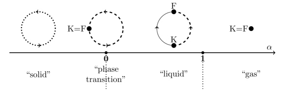
Figure 1: Schematic illustration of the renormalization group flow on the spaces of self-adjoint realizations of Bessel operators. It is borrowed from [9]. Heavy dots represent fixed points. The letters $K$ and $F$ correspond to the Krein and Friedrichs extensions of $L_{\alpha}^{\min}$. Dashed lines represent realizations with a single bound state. Dotted line represents an infinite number of bound states. The arrow indicates the direction of the flow.

The names of the various phases can be treated as jokes. One can also try to justify them as follows. For $\alpha>1$ the space of realizations is trivial. This is the simplest phase—hence the name ”gas”. For $\alpha<0$ the continuous scaling symmetry is broken to a discrete subgroup, as in crystals—this justifies the name “solid”. The intermediate situation, $0<\alpha<1$ is consequently called the “liquid phase”.

3 “Wilsonian approach” to inverse square potential

In this section we give a partly heuristic theory of Bessel operators in the spirit of the Wilsonian renormalization. We will mostly follow the presentation of [7], preserving to a large extent its style and language. In the next section we give a rigorous description of all steps of this section.

For a description of the Wilsonian renormalization procedure applied to quantum field theory the reader can consult [12, 13, 26].

The main object of the analysis of [7] is the formal expression

$$\tilde{L}_{\alpha,3}\psi(\vec{p})=|\vec{p}|^{2}\psi(\vec{p})+\frac{1}{4\pi}\Big{(}\alpha-\frac{1}{4}\Big{)}\int d^{3}\vec{q}\frac{1}{|\vec{p}-\vec{q}|}\psi(\vec{q}).$$ (3.1)

Formally, it is the momentum representation of

$$L_{\alpha,3}:=-\Delta_{3}+\Big{(}\alpha-\frac{1}{4}\Big{)}\frac{1}{r^{2}},$$ (3.2)

where $\Delta_{3}$ is the $3$-dimensional Laplacian and $r$ is the radial coordinate.

More precisely, if $\mathcal{F}f(\vec{p})$ is the Fourier transform of $f(\vec{x})$, then

$$\tilde{L}_{\alpha,3}:=\mathcal{F}L_{\alpha,3}\mathcal{F}^{-1}.$$ (3.3)

Let us note that the 3-dimensional formulation is equivalent to the 1-dimensional one. Indeed, every $\psi\in L^{2}(\mathbb{R}^{3})$ can be written in spherical coordinates $r,\vartheta,\phi$ as

$$\psi=\sum_{l=0}^{\infty}\sum_{m=-l}^{l}Y_{l,m}(\vartheta,\phi)\frac{1}{r}f_{l,m}(r),$$

where $Y_{l,m}$ are spherical harmonics. It follows that on $l$ degree spherical harmonics $L_{\alpha,3}$ is equivalent to

$$-\partial_{r}^{2}+\Big{(}(l+1/2)^{2}+\alpha-\frac{1}{2}\Big{)}\frac{1}{r^{2}}.$$

For further convenience let us denote $p:=|\vec{p}|$. We will restrict our attention to the s-wave sector, that is, to spherically symmetric functions. In the s-wave sector we can write $\psi(\vec{p})=\psi(p)$ with $p:=|\vec{p}|$ and the operator Eq. (3.1) can be written in the following way (see Eqs. (3) and (4) in [7]):

$$\tilde{L}_{\alpha}\psi(p)=p^{2}\psi(p)+\Big{(}\alpha-\frac{1}{4}\Big{)}\int_{0}^{\infty}\mathrm{d}q\>q^{2}\Big{(}\theta(p-q)p^{-1}+\theta(q-p)q^{-1}\Big{)}\psi(q),$$ (3.4)

where $\theta(x)$ denotes the Heaviside step function and we dropped $3$ from the subscript.

Unfortunately, (3.4) does not define a Hermitian operator. To find a self-adjoint realisation, we introduce an ultraviolet cutoff $\Lambda$ and a counter-term $\frac{f_{\Lambda}}{\Lambda}$. Thus we consider a family of cutoff Hamiltonians

$$\tilde{H}_{\alpha}(\Lambda,f_{\Lambda})\psi(p)\coloneqq\begin{cases}p^{2}\psi(p)+\int_{0}^{\Lambda}\mathrm{d}q\>q^{2}\Big{(}V(p,q)+\frac{f_{\Lambda}}{\Lambda}\Big{)}\psi(q),&\mathrm{for}\>p\leq\Lambda\\ 0,&\mathrm{for}\>p>\Lambda.\end{cases}$$ (3.5)

where

$$V(p,q)=\Big{(}\alpha-\frac{1}{4}\Big{)}\Big{(}\theta(p-q)p^{-1}+\theta(q-p)q^{-1}\Big{)}.$$ (3.6)

Let $\tilde{U}$ denote the dilation in the momentum representation, that is

$$\tilde{U}(\tau)\mathcal{F}=\mathcal{F}U(\tau).$$ (3.7)

Note that in the momentum representation the dilation acts in the opposite way than in the position representation:

$$\tilde{U}(\tau)\psi(p)=\mathrm{e}^{-\frac{3}{2}\tau}\psi(\mathrm{e}^{-\tau}p).$$ (3.8)

It is easy to see that

$$\tilde{U}(\tau)\tilde{H}_{\alpha}(\Lambda,f_{\Lambda})\tilde{U}(-\tau)=\mathrm{e}^{-2\tau}\tilde{H}_{\alpha}(\mathrm{e}^{\tau}\Lambda,f_{\Lambda}).$$ (3.9)

Thus changing $\Lambda$ can be interpreted as the change of a scale.

We would like to find out for what kind of dependence of $f_{\Lambda}$ on $\Lambda$ we can expect the existence of a limit $H_{\alpha}(\Lambda,f_{\Lambda})$ for $\Lambda\to\infty$ as a self-adjoint operator. To this end we assume that we have a fixed eigenfunction $\psi$ satisfying

$$H_{\alpha}(\Lambda,f_{\Lambda})\psi(p)=E\psi(p),\quad p<\Lambda.$$ (3.10)

Following the terminology of [7], we will say that two Hamiltonians $\tilde{H}_{m}(\Lambda,f_{\Lambda})$ and $\tilde{H}_{\alpha}(\Lambda^{\prime},f_{\Lambda^{\prime}})$ are equivalent if

$$\tilde{H}_{\alpha}(\Lambda,f_{\Lambda})\psi(p)=\tilde{H}_{\alpha}(\Lambda^{\prime},f_{\Lambda^{\prime}})\psi(p)\quad\mathrm{for}\>p<\mathrm{min}(\Lambda,\Lambda^{\prime}).$$

Two Hamiltonians are equivalent if the function $\gamma(\Lambda)\equiv f_{\Lambda}/\Lambda$ satisfies the equation

$$\frac{\mathrm{d}\gamma(\Lambda)}{\mathrm{d}\Lambda}=\Big{[}\gamma(\Lambda)-\frac{1/4-\alpha}{\Lambda}\Big{]}^{2}.$$ (3.11)

To prove it, we consider an infinitesimal reduction of the cut-off $\Lambda\rightarrow\Lambda-\mathrm{d}\Lambda$. Let $\psi$ be a solution of

$$\tilde{H}_{\alpha}(\Lambda,f_{\Lambda})\psi(p)=-k^{2}\psi(p).$$ (3.12)

By splitting the integral

$$\int_{0}^{\Lambda}\mathrm{d}q\>q^{2}\Big{(}V(p,q)+\gamma(\Lambda)\Big{)}\psi(q)\approx\int_{0}^{\Lambda-d\Lambda}\mathrm{d}q\>q^{2}\Big{(}V(p,q)+\gamma(\Lambda)\Big{)}\psi(q)+\mathrm{d}\Lambda\Big{(}V(p,\Lambda)+\gamma(\Lambda)\Big{)}\psi({\Lambda}),$$

and using the relation resulting from Eqs. (3.5) and (3.12):

$$\psi(\Lambda)=-\frac{1}{k^{2}+\Lambda^{2}}\int_{0}^{\Lambda}\mathrm{d}q\>q^{2}\Big{(}(\alpha-\frac{1}{4})\Lambda^{-1}+\gamma(\Lambda)\Big{)}\psi(q),$$

assuming the large cut-off $k^{2}\ll\Lambda^{2}$ we conclude that the Hamiltonian $\tilde{H}_{\alpha}(\Lambda,f_{\Lambda})$ is equivalent to $\tilde{H}_{\alpha}(\Lambda-\mathrm{d}\Lambda,f_{\Lambda-\mathrm{d}\Lambda})$ such that

$$\tilde{H}_{\alpha}(\Lambda-\mathrm{d}\Lambda,f_{\Lambda-\mathrm{d}\Lambda})\psi(p)\coloneqq p^{2}\psi(p)+\int_{0}^{\Lambda-\mathrm{d}\Lambda}\mathrm{d}q\>q^{2}\Big{(}V(p,q)+\gamma(\Lambda-\mathrm{d}\Lambda)\Big{)}\psi(q),$$

where

$$\gamma(\Lambda-\mathrm{d}\Lambda)=\gamma(\Lambda)-\mathrm{d}\Lambda\Big{[}\gamma(\Lambda)-\frac{1/4-\alpha}{\Lambda}\Big{]}^{2}.$$ (3.13)

Taking the limit $\mathrm{d}\Lambda\rightarrow 0$ we obtain the differential equation (3.11). Its solutions are of the form $\gamma(\Lambda)=\Lambda^{-1}f_{\Lambda}$. Let us analyze the flow $\Lambda\to f_{\Lambda}$.

• For $\alpha<0$, we set $m_{I}:=\sqrt{-\alpha}$,

  $$f_{\Lambda}=m_{I}\tan\bigg{(}\arctan\Big{(}\frac{f_{\Lambda_{0}}-m_{I}^{2}+1/4}{m_{I}}\Big{)}+m_{I}\log\frac{\Lambda}{\Lambda_{0}}\bigg{)}+m_{I}^{2}-\frac{1}{4}.$$ (3.14)

  There are no fixed points. Moreover, there is a discrete scaling symmetry: for any $n\in\mathbb{Z}$, Hamiltonians $\tilde{H}(\Lambda,f_{\Lambda})$ and $\tilde{H}(\Lambda\cdot\exp(\pi n/m_{I}),f_{\Lambda})$ are equivalent.

• For $\alpha=0$,

  $$f_{\Lambda}=\frac{f_{\Lambda_{0}}+1/4}{1-(f_{\Lambda_{0}}+1/4)\log\frac{\Lambda}{\Lambda_{0}}}-\frac{1}{4}.$$ (3.15)

  There is one fixed point corresponding to $f_{\Lambda_{0}}=-1/4$, for which Hamiltonians $\tilde{H}_{m}(\Lambda,f_{\Lambda_{0}})$ are equivalent for all values of $\Lambda$.

• for $\alpha>0$, we set $m:=\sqrt{\alpha}>0$

  $$f_{\Lambda}=-m\tanh\bigg{(}-\mathrm{atanh}\Big{(}\frac{f_{\Lambda_{0}}+m^{2}+1/4}{m}\Big{)}+m\log\frac{\Lambda}{\Lambda_{0}}\bigg{)}-m^{2}-\frac{1}{4}.$$ (3.16)

  There are two fixed point: an attractive one $f_{\Lambda_{0}}^{+}=-\big{(}m+\frac{1}{2}\big{)}^{2}$ and a repulsive one $f_{\Lambda_{0}}^{-}=\big{(}m-\frac{1}{2}\big{)}^{2}$, for which Hamiltonians $\tilde{H}_{m}(\Lambda,f^{\pm}_{\Lambda_{0}})$ are equivalent for all values of $\Lambda$.

We thus reproduce the the three first pictures from Figure 1.

4 Momentum approach

4.1 Momentum approach to Schrödinger operators on $\mathbb{R}^{d}$

Self-adjoint operators on $L^{2}(\mathbb{R}^{d})$ of the form

$$H=-\Delta+V(x)$$ (4.1)

are usually called Schrödinger operators. They are typically studied by methods of the configuration space. However, they can also be approached from the momentum point of view.

We will typically use $x\in\mathbb{R}^{d}$ for the generic variable in the position representation and $p\in\mathbb{R}^{d}$ in the momentum representation. Let us recall the two most common conventions for the Fourier transformation:

$$\tilde{f}(p) :=\int\mathrm{e}^{-\mathrm{i}xp}f(x)\mathrm{d}x,$$ (4.2)

$$\mathcal{F}f(p) :=(2\pi)^{-\frac{d}{2}}\int\mathrm{e}^{-\mathrm{i}xp}f(x)\mathrm{d}x=(2\pi)^{-\frac{d}{2}}\tilde{f}(p).$$ (4.3)

Note that $\mathcal{F}$ is unitary. Let $\tilde{H}$ denote the operator $H$ in the momentum representation, that is

$$\tilde{H}:=\mathcal{F}H\mathcal{F}^{-1}.$$ (4.4)

If the potential $V$ is well-behaved, then $\tilde{H}$ can be written as

$$\tilde{H}\psi(p)=p^{2}\psi(p)+(2\pi)^{-d}\int\tilde{V}(p-q)\psi(q)\mathrm{d}q.$$ (4.5)

4.2 Momentum approach to Schrödinger operators on $\mathbb{R}_{+}$

Often we consider Schrödinger operators on a subset of $\mathbb{R}^{d}$. Then the representation (4.5) becomes problematic, because it needs to take into account the boundary conditions. Besides, it is not obvious what should replace the Fourier transformation.

A case of particular interest is $\mathbb{R}_{+}$. In this case we have two distinguished realizations of the 1-dimensional Laplacian: the Dirichlet Laplacian $\Delta_{\mathrm{D}}$ and the Neumann Laplacian $\Delta_{\mathrm{N}}$. Instead of the Fourier transformation it is natural to use the sine transformation $\mathcal{F}_{\mathrm{D}}$ or the cosine transformation $\mathcal{F}_{\mathrm{N}}$:

$$(\mathcal{F}_{\mathrm{D}}f)(p) :=\sqrt{\frac{2}{\pi}}\int_{0}^{\infty}\sin(px)f(x)\mathrm{d}x,$$ (4.6)

$$(\mathcal{F}_{\mathrm{N}}f)(p) :=\sqrt{\frac{2}{\pi}}\int_{0}^{\infty}\cos(px)f(x)\mathrm{d}x.$$ (4.7)

Both are involutions, that is,

$$\mathcal{F}_{\mathrm{D}}^{2}\psi=\mathcal{F}_{\mathrm{N}}^{2}\psi=\psi,$$ (4.8)

they are unitary and diagonalize the Dirichlet/Neumann Laplacian:

$$\mathcal{F}_{\mathrm{D}}(-\Delta_{\mathrm{D}})\mathcal{F}_{\mathrm{D}}\psi(p) =p^{2}\psi(p),$$ (4.9)

$$\mathcal{F}_{\mathrm{N}}(-\Delta_{\mathrm{N}})\mathcal{F}_{\mathrm{N}}\psi(p) =p^{2}\psi(p).$$ (4.10)

Consider now a Schrödinger operator on the half-line with a potential $V$. Let us first assume that $V$ is sufficiently regular, say, $V\in L^{1}(\mathbb{R}_{+})$. Then one can impose the Dirichlet or Neumann boundary conditions at $0$, so that one has two Schrödinger operators

$$H_{\mathrm{D}} :=-\Delta_{\mathrm{D}}+V(x),$$ (4.11)

$$H_{\mathrm{N}} :=-\Delta_{\mathrm{N}}+V(x).$$ (4.12)

As suggested by Eqs. (4.9)-(4.10), to obtain their momentum versions it is natural to apply the sine transform to the first and the cosine transform to the second Hamiltonian:

$$\tilde{H}_{\mathrm{D}} :=\mathcal{F}_{\mathrm{D}}H_{\mathrm{D}}\mathcal{F}_{\mathrm{D}},$$ (4.13)

$$\tilde{H}_{\mathrm{N}} :=\mathcal{F}_{\mathrm{N}}H_{\mathrm{N}}\mathcal{F}_{\mathrm{N}}.$$ (4.14)

Let us extend the potential $V$ to an even function on the whole $\mathbb{R}$, so that $V(-x)=V(x)$. Let $\tilde{V}(p)$ be the Fourier transform of $V$, as in (4.2). Then (4.13) and (4.14) are given by the following expressions, which easily follow from (4.5) and (A.7):

$$\tilde{H}_{\mathrm{D}}\psi(p)=p^{2}\psi(p)+\frac{1}{2\pi}\int_{0}^{\infty}(\tilde{V}(p-q)-\tilde{V}(p+q)\big{)}\psi(q)\mathrm{d}q,$$ (4.15)

$$\tilde{H}_{\mathrm{N}}\psi(p)=p^{2}\psi(p)+\frac{1}{2\pi}\int_{0}^{\infty}(\tilde{V}(p-q)+\tilde{V}(p+q)\big{)}\psi(q)\mathrm{d}q.$$ (4.16)

4.3 Minimal realization in the momentum approach

A priori it is not obvious which transformation is more appropriate for the Bessel operator: the sine or the cosine transformation. Let us consider both, setting

$$\tilde{L}_{\alpha,\mathrm{D}} :=\mathcal{F}_{\mathrm{D}}L_{\alpha}\mathcal{F}_{\mathrm{D}},$$ (4.17)

$$\tilde{L}_{\alpha,\mathrm{N}} :=\mathcal{F}_{\mathrm{N}}L_{\alpha}\mathcal{F}_{\mathrm{N}},$$ (4.18)

(where, as before, $L_{\alpha}$ is treated as a formal expression).

Then, using $-\pi|p|$ as the Fourier transform of $\frac{1}{x^{2}}$, (4.15) and (4.16) yield

$$\tilde{L}_{\alpha,\mathrm{D}}\psi(p) =p^{2}\psi(p)+\Big{(}\alpha-\frac{1}{4}\Big{)}\int_{0}^{\infty}\big{(}\theta(p-q)q+\theta(q-p)p\big{)}\psi(q)\mathrm{d}q,$$ (4.19)

$$\tilde{L}_{\alpha,\mathrm{N}}\psi(p) =p^{2}\psi(p)-\Big{(}\alpha-\frac{1}{4}\Big{)}\int_{0}^{\infty}\big{(}\theta(p-q)p+\theta(q-p)q\big{)}\psi(q)\mathrm{d}q.$$ (4.20)

So far, we have treated $\tilde{L}_{\alpha,\mathrm{D}}$ and $\tilde{L}_{\alpha,\mathrm{N}}$ as formal expressions. We would like to make them well defined, first in the “minimal sense”.

In the position representation, an easy way to make the expression $L_{\alpha}$ well defined was to restrict its domain to $C_{\mathrm{c}}^{\infty}(\mathbb{R}_{+})$, which after the closure led to the minimal realisation. Of course, it was not necessary to demand that the support is away from zero, however functions in the domain should have vanished of an appropriate order at zero. In the momentum representation it is useful to restrict the domain to rapidly decaying functions—in the position representation this guarantees the smoothness. On the position side, this also guarantees that even/odd derivatives at zero vanish in the Dirichlet, resp. Neumann case, see (A.14). This does not suffice—in addition, we need to impose conditions that on the position side yield vanishing first/zeroth derivative. Thus, we introduce the spaces (see Appx A):

$$L_{j}^{2,\infty}(\mathbb{R}_{+}):=\left\{\psi\in L^{2,\infty}(\mathbb{R}_{+})\ |\ \int_{0}^{\infty}|\psi(p)|^{2}p^{n}\mathrm{d}p<\infty,\quad n=0,1,\dots;\quad\int_{0}^{\infty}\psi(p)p^{j}\mathrm{d}p=0\right\},\quad j=0,1.$$ (4.21)

Theorem 4.1

1. The operator $\tilde{L}_{\alpha,\mathrm{D}}$ given by the formula (4.19) restricted to $L_{1}^{2,\infty}(\mathbb{R}_{+})$ is well defined and closable. Let us denote its closure by $\tilde{L}_{\alpha,\mathrm{D}}^{\min}$. We then have

   $$\tilde{L}_{\alpha,\mathrm{D}}^{\min} :=\mathcal{F}_{\mathrm{D}}L_{\alpha}^{\min}\mathcal{F}_{\mathrm{D}}.$$ (4.22)

2. The operator $\tilde{L}_{\alpha,\mathrm{N}}$ given by the formula (4.20) restricted to $L_{0}^{2,\infty}(\mathbb{R}_{+})$ is well defined and closable. Let us denote its closure by $\tilde{L}_{\alpha,\mathrm{N}}^{\min}$. Then we have

   $$\tilde{L}_{\alpha,\mathrm{N}}^{\min} :=\mathcal{F}_{\mathrm{N}}L_{\alpha}^{\min}\mathcal{F}_{\mathrm{N}}.$$ (4.23)

Proof. Consider first the Dirichlet case. Let $\psi\in L_{1}^{2,\infty}(\mathbb{R}_{+})$ and $x>0$. Consider

$$\phi(p) :=\int_{0}^{\infty}\big{(}\theta(p-q)q+\theta(q-p)p\big{)}\psi(q)\mathrm{d}q=\int_{p}^{\infty}(p-q)\psi(q)\mathrm{d}q,$$ (4.24)

where in the last transition we used the property of Eq. (4.21). Clearly, $\phi(0)=0$ and $\lim\limits_{p\to\infty}\phi(p)=0$. Moreover,

$$\phi^{\prime}(p)=\int_{p}^{\infty}\psi(q)\mathrm{d}q$$ (4.25)

and $\lim\limits_{p\to\infty}\phi^{\prime}(p)=0$. We can integrate twice obtaining

$$\int_{0}^{\infty}\sin(px)\phi(p)\mathrm{d}p =\frac{1}{x}\int_{0}^{\infty}\cos(px)\phi^{\prime}(p)\mathrm{d}p$$ (4.26)

$$=\frac{1}{x^{2}}\int_{0}^{\infty}\sin(px)\psi(p)\mathrm{d}p.$$ (4.27)

By (A.15),

$$\int_{0}^{\infty}\sin(px)p^{2}\phi(p)\mathrm{d}p =-\partial_{x}^{2}\int_{0}^{\infty}\sin(px)\phi(p)\mathrm{d}p.$$ (4.28)

Therefore,

$$\mathcal{F}_{\mathrm{D}}\tilde{L}_{\alpha,\mathrm{D}}\psi=L_{\alpha}\mathcal{F}_{\mathrm{D}}\psi.$$ (4.29)

Thus $\mathcal{F}_{\mathrm{D}}\tilde{L}_{\alpha,\mathrm{D}}\mathcal{F}_{\mathrm{D}}$ coincides with $L_{\alpha}$ on $\mathcal{F}_{\mathrm{D}}L_{1}^{2,\infty}(\mathbb{R}_{+})$.

Suppose now that $\phi=\mathcal{F}_{\mathrm{D}}\psi$ with $\psi\in L_{1}^{2,\infty}(\mathbb{R}_{+})$. We have $\phi^{(n)}(0)=0$, $n=0,2,\dots$ (by (A.14), because $\psi\in L^{2,\infty}(\mathbb{R}_{+})$). Moreover, $\phi^{\prime}(0)=0$ (by (A.16), because $\int\limits_{0}^{\infty}p\psi(p)\mathrm{d}p=0$). Hence $\phi(x)=O(x^{3})$.

Let $\chi,\xi\in C^{\infty}(\mathbb{R}_{+})$, $\chi=1$, $\xi=0$ near $0$ and $\chi=0$, $\xi=1$ near $\infty$. Set $\phi_{\epsilon}(x):=\chi(x/\epsilon)\xi(x\epsilon)\psi(x)$. Then we easily show that $\|L_{\alpha}(\phi-\phi_{\epsilon})\|^{2}+\|\phi-\phi_{\epsilon}\|^{2}\to 0$ as $\epsilon\rightarrow 0$. Clearly, $\phi_{\epsilon}\in C_{\mathrm{c}}^{\infty}(\mathbb{R}_{+})$. Therefore $\mathcal{F}_{\mathrm{D}}L_{1}^{2,\infty}(\mathbb{R}_{+})\subset\mathcal{D}(L_{\alpha}^{\min})$.

Clearly, $C_{\mathrm{c}}^{\infty}(\mathbb{R}_{+})\subset\mathcal{F}_{\mathrm{D}}L_{1}^{2,\infty}(\mathbb{R}_{+})$. Therefore, $\mathcal{F}_{\mathrm{D}}L_{1}^{2,\infty}(\mathbb{R}_{+})$ is dense in $\mathcal{D}(L_{\alpha}^{\min})$.

This proves that the closure of $\mathcal{F}_{\mathrm{D}}\tilde{L}_{\alpha,\mathrm{D}}\mathcal{F}_{\mathrm{D}}$ restricted to $\mathcal{F}_{\mathrm{D}}L_{1}^{2,\infty}(\mathbb{R}_{+})$ coincides with $L_{\alpha}^{\min}$.

Consider next the Neumann case. Let $\psi\in L_{0}^{2,\infty}(\mathbb{R}_{+})$. Consider

$$\phi(p) :=\int_{0}^{\infty}\mathrm{d}q\big{(}\theta(p-q)p+\theta(q-p)q\big{)}\psi(q)=\int_{p}^{\infty}(q-p)\psi(q)\mathrm{d}q.$$ (4.30)

Clearly, $\lim\limits_{p\to\infty}\phi(p)=0$. Moreover,

$$\phi^{\prime}(p)=\int_{0}^{p}\psi(q)\mathrm{d}q$$ (4.31)

and $\phi^{\prime}(p)=0$, $\lim\limits_{p\to\infty}\phi^{\prime}(p)=0$. We can integrate twice obtaining

$$\int_{0}^{\infty}\cos(px)\phi(p)\mathrm{d}p =-\frac{1}{x}\int_{0}^{\infty}\sin(px)\phi^{\prime}(p)\mathrm{d}p$$ (4.32)

$$={-}\frac{1}{x^{2}}\int_{0}^{\infty}\cos(px)\psi(p)\mathrm{d}p.$$ (4.33)

Clearly,

$$\int_{0}^{\infty}\cos(px)p^{2}\phi(p)\mathrm{d}p =-\partial_{x}^{2}\int_{0}^{\infty}\cos(px)\phi(p)\mathrm{d}p.$$ (4.34)

Therefore

$$\mathcal{F}_{\mathrm{N}}\tilde{L}_{\alpha,\mathrm{N}}\psi=L_{\alpha}\mathcal{F}_{\mathrm{N}}\psi.$$ (4.35)

Thus $\mathcal{F}_{\mathrm{N}}\tilde{L}_{\alpha,\mathrm{N}}\mathcal{F}_{\mathrm{N}}$ coincides with $L_{\alpha}$ on $\mathcal{F}_{\mathrm{N}}L_{0}^{2,\infty}(\mathbb{R}_{+})$.

Suppose now that $\phi=\mathcal{F}_{\mathrm{N}}\psi$ with $\psi\in L_{0}^{2,\infty}(\mathbb{R}_{+})$. We have $\phi^{(n)}(0)=0$, $n=1,3,\dots$ (because $\psi\in L^{2,\infty}(\mathbb{R}_{+})$). Moreover, $\phi(0)=0$ (because $\int\limits_{0}^{\infty}\psi(p)\mathrm{d}p=0$). Hence $\phi(x)=O(x^{2})$.

The remaining arguments are the same as in the Dirichlet case. $\Box$

4.4 Maximal realization in the momentum approach

In this subsection we present a construction of the maximal operator $L_{\alpha}^{\max}$ for $\alpha<1$. The construction involves two steps:

1. the choice of two vectors that together with $\mathcal{D}(L_{\alpha}^{\min})$ span $\mathcal{D}(L_{\alpha}^{\max})$;

2. the action of $L_{\alpha}^{\max}$ on these two vectors.

We will first describe the construction for the generic case $\alpha\neq\frac{1}{4}$. Let $\alpha<1$, and $\alpha=m^{2}$. As we remember, if $\alpha\neq 0$, elements of $\mathcal{D}(L^{\mathrm{max}}_{\alpha})$ behave like $c_{+}x^{1/2+m}+c_{-}x^{1/2-m}$ as $x\rightarrow 0$. By (A.18) and (A.19), the sine and cosine transforms of $x^{\frac{1}{2}\pm m}$ are proportional to $p^{-\frac{3}{2}\mp m}$. This suggests to enlarge the domain of the minimal operators by functions that behave like $p^{-\frac{3}{2}\mp m}$ as $p\rightarrow\infty$. However, we cannot simply take $p^{-\frac{3}{2}\mp m}$, because they are not square integrable near zero. This complicates the whole story. (For $\alpha=0$, additionally, we need to modify all this using the logarithm.)

More precisely, let us fix $\psi_{\pm m,\mathrm{D}}$, $\psi_{\pm m,\mathrm{N}}$, $\psi_{\log,\mathrm{D}}$ and $\psi_{\log,\mathrm{N}}$ be functions in $L^{2}(\mathbb{R}_{+})$ satisfying the following condition: there exists $\Lambda_{0}>0$ such that

$$p>\Lambda_{0}\ \Rightarrow\quad\psi_{\pm m,\mathrm{D}}(p)=p^{-\frac{3}{2}\mp m}, \qquad\int_{0}^{\Lambda_{0}}\psi_{\pm m,\mathrm{D}}(q)q\mathrm{d}q=\frac{\Lambda_{0}^{\frac{1}{2}\mp m}}{\frac{1}{2}\mp m},\quad{m\neq\pm\frac{1}{2}},$$ (4.36)

$$p>\Lambda_{0}\ \Rightarrow\quad\psi_{\log,\mathrm{D}}(p)=p^{-\frac{3}{2}}\log(p), \qquad\int_{0}^{\Lambda_{0}}\psi_{\log,\mathrm{D}}(q)q\mathrm{d}q=-4\Lambda_{0}^{\frac{1}{2}}+2\Lambda_{0}^{\frac{1}{2}}\log\Lambda_{0},$$ (4.37)

$$p>\Lambda_{0}\ \Rightarrow\quad\psi_{\pm m,\mathrm{N}}(p)=p^{-\frac{3}{2}\mp m}, \qquad\int_{0}^{\Lambda_{0}}\psi_{\pm m,\mathrm{N}}(q)\mathrm{d}q=\frac{\Lambda_{0}^{-\frac{1}{2}\mp m}}{-\frac{1}{2}\mp m},\quad{m\neq\mp\frac{1}{2}},$$ (4.38)

$$p>\Lambda_{0}\ \Rightarrow\quad\psi_{\log,\mathrm{N}}(p)=p^{-\frac{3}{2}}\log(p), \qquad\int_{0}^{\Lambda_{0}}\psi_{\log,\mathrm{N}}(q)\mathrm{d}q=-4\Lambda_{0}^{-\frac{1}{2}}-2\Lambda_{0}^{-\frac{1}{2}}\log\Lambda_{0}.$$ (4.39)

Note that (4.36) and (4.38) imply

$$\Lambda>\Lambda_{0}\ \Rightarrow \int_{0}^{\Lambda}\psi_{\pm m,\mathrm{D}}(q)q\mathrm{d}q=\frac{\Lambda^{\frac{1}{2}\mp m}}{\frac{1}{2}\mp m},\quad{m\neq\pm\frac{1}{2}},$$ (4.40)

$$\Lambda>\Lambda_{0}\ \Rightarrow \int_{0}^{\Lambda}\psi_{\log,\mathrm{D}}(q)q\mathrm{d}q=-4\Lambda^{\frac{1}{2}}+2\Lambda^{\frac{1}{2}}\log\Lambda,$$ (4.41)

$$\Lambda>\Lambda_{0}\ \Rightarrow \int_{0}^{\Lambda}\psi_{\pm m,\mathrm{N}}(q)\mathrm{d}q=\frac{\Lambda^{-\frac{1}{2}\mp m}}{-\frac{1}{2}\mp m},\quad{m\neq\mp\frac{1}{2}},$$ (4.42)

$$\Lambda>\Lambda_{0}\ \Rightarrow \int_{0}^{\Lambda}\psi_{\log,\mathrm{N}}(q)\mathrm{d}q=-4\Lambda^{-\frac{1}{2}}-2\Lambda^{-\frac{1}{2}}\log\Lambda.$$ (4.43)

We set

$$\mathcal{D}(\tilde{L}_{\alpha,\mathrm{D}}^{\max}) :=\mathcal{D}(\tilde{L}_{\alpha,\mathrm{D}}^{\min})+\mathbb{C}\psi_{m,\mathrm{D}}+\mathbb{C}\psi_{-m,\mathrm{D}},\quad{\alpha\neq\frac{1}{4}}$$ (4.44)

$$\mathcal{D}(\tilde{L}_{0,\mathrm{D}}^{\max}) :=\mathcal{D}(\tilde{L}_{0,\mathrm{D}}^{\min})+\mathbb{C}\psi_{0,\mathrm{D}}+\mathbb{C}\psi_{\log,\mathrm{D}}$$ (4.45)

$$\mathcal{D}(\tilde{L}_{\alpha,\mathrm{N}}^{\max}) :=\mathcal{D}(\tilde{L}_{\alpha,\mathrm{N}}^{\min})+\mathbb{C}\psi_{m,\mathrm{N}}+\mathbb{C}\psi_{-m,\mathrm{N}},\quad{\alpha\neq\frac{1}{4}},$$ (4.46)

$$\mathcal{D}(\tilde{L}_{0,\mathrm{N}}^{\max}) :=\mathcal{D}(\tilde{L}_{0,\mathrm{N}}^{\min})+\mathbb{C}\psi_{0,\mathrm{N}}+\mathbb{C}\psi_{\log,\mathrm{N}}.$$ (4.47)

Clearly, the difference of two functions satisfying (4.36), (4.37), (4.38) or (4.39), belongs to $L_{1}^{2,\infty}(\mathbb{R}_{+})$, resp to $L_{0}^{2,\infty}(\mathbb{R}_{+})$. Therefore, (4.44), (4.46), (4.45) and (4.47) do not depend on the choices of $\psi_{\pm m,\mathrm{D}}$ and $\psi_{\pm m,\mathrm{N}}$.

The formulas (4.19) and (4.20) are in general ill defined on (4.44), (4.46), (4.45) and (4.47), because the integrals can be divergent at $\infty$. In order to define the maximal operators in the momentum representation, we note that every $\psi$ in $\mathcal{D}(\tilde{L}_{\alpha,\mathrm{D}}^{\max})$ or in $\mathcal{D}(\tilde{L}_{\alpha,\mathrm{N}}^{\max})$ behaves like

$$\psi(p)\sim\tilde{c}_{+}p^{-\frac{3}{2}-m}+\tilde{c}_{-}p^{-\frac{3}{2}+m},\quad p\rightarrow\infty,$$ (4.48)

$$\text{ resp.}\qquad\psi(p)\sim\tilde{c}_{+}p^{-\frac{3}{2}}\log(p)+\tilde{c}_{-}p^{-\frac{3}{2}},\quad p\rightarrow\infty,$$ (4.49)

for some uniquely defined $\tilde{c}_{+},\tilde{c}_{-}$. Then for $\alpha\neq\frac{1}{4}$ we set

$$\tilde{L}_{\alpha,\mathrm{D}}^{\max}\psi(p) =p^{2}\psi(p)+\Big{(}\alpha-\frac{1}{4}\Big{)}\lim_{\Lambda\to\infty}\Bigg{(}\int_{0}^{\Lambda}\mathrm{d}q\big{(}\theta(p-q)q+\theta(q-p)p\big{)}\psi(q)+\frac{\tilde{c}_{+}p\Lambda^{-\frac{1}{2}-m}}{\frac{1}{2}+m}+\frac{\tilde{c}_{-}p\Lambda^{-\frac{1}{2}+m}}{\frac{1}{2}-m}\Bigg{)},$$ (4.50)

$$\tilde{L}_{0,\mathrm{D}}^{\max}\psi(p) =p^{2}\psi(p)-\frac{1}{4}\lim_{\Lambda\to\infty}\Bigg{(}\int_{0}^{\Lambda}\mathrm{d}q\big{(}\theta(p-q)q+\theta(q-p)p\big{)}\psi(q)+\tilde{c}_{+}p\big{(}4\Lambda^{-\frac{1}{2}}+2\Lambda^{-\frac{1}{2}}\log\Lambda\big{)}+2\tilde{c}_{-}p\Lambda^{-\frac{1}{2}}\Bigg{)},$$ (4.51)

$$\tilde{L}_{\alpha,\mathrm{N}}^{\max}\psi(p) =p^{2}\psi(p)-\Big{(}\alpha-\frac{1}{4}\Big{)}\lim_{\Lambda\to\infty}\Bigg{(}\int_{0}^{\Lambda}\mathrm{d}q\big{(}\theta(p-q)p+\theta(q-p)q\big{)}\psi(q)-\frac{\tilde{c}_{+}\Lambda^{\frac{1}{2}-m}}{\frac{1}{2}-m}-\frac{\tilde{c}_{-}\Lambda^{\frac{1}{2}+m}}{\frac{1}{2}+m}\Bigg{)},$$ (4.52)

$$\tilde{L}_{0,\mathrm{N}}^{\max}\psi(p) =p^{2}\psi(p){+}\frac{1}{4}\lim_{\Lambda\to\infty}\Bigg{(}\int_{0}^{\Lambda}\mathrm{d}q\big{(}\theta(p-q)p+\theta(q-p)q\big{)}\psi(q)+\tilde{c}_{+}\big{(}4\Lambda^{\frac{1}{2}}-2\Lambda^{\frac{1}{2}}\log\Lambda\big{)}-2\tilde{c}_{-}\Lambda^{\frac{1}{2}}\Bigg{)}.$$ (4.53)

Note that in the Dirichlet case with $\alpha<\frac{1}{4}$ (and hence $|\mathrm{Re}(m)|<\frac{1}{2}$) both counterterms in (4.50) are not necessary—they go to zero and the integrals are convergent. However in all other cases at least one counterterm is needed.

Theorem 4.2

Let $\alpha<1$ and $\alpha\neq\frac{1}{4}$. The operators $\tilde{L}_{\alpha,\mathrm{D}}^{\max}$ and $\tilde{L}_{\alpha,\mathrm{N}}^{\max}$ are well defined closed operators. We have

$$\tilde{L}_{\alpha,\mathrm{D}}^{\max} :=\mathcal{F}_{\mathrm{D}}L_{\alpha}^{\max}\mathcal{F}_{\mathrm{D}},$$ (4.54)

$$\tilde{L}_{\alpha,\mathrm{N}}^{\max} :=\mathcal{F}_{\mathrm{N}}L_{\alpha}^{\max}\mathcal{F}_{\mathrm{N}}.$$ (4.55)

Proof. Consider first the Dirichlet case. It is enough to consider $\psi=\psi_{\pm m,\mathrm{D}}$

$$p^{2}\psi(p)+\Big{(}\alpha-\frac{1}{4}\Big{)}\lim_{\Lambda\to\infty}\Bigg{(}\int_{0}^{\Lambda}\mathrm{d}q\big{(}\theta(p-q)q+\theta(q-p)p\big{)}\psi(q)+\frac{p\Lambda^{-\frac{1}{2}\mp m}}{\frac{1}{2}\pm m}\Bigg{)}$$ (4.56)

$$=p^{2}\psi(p)+\Big{(}\alpha-\frac{1}{4}\Big{)}\lim_{\Lambda\to\infty}\Bigg{(}\int_{p}^{\Lambda}\mathrm{d}q(p-q)\psi(q)+\frac{p\Lambda^{-\frac{1}{2}\mp m}}{\frac{1}{2}\pm m}+\frac{\Lambda^{\frac{1}{2}\mp m}}{\frac{1}{2}\mp m}\Bigg{)}$$ (4.57)

$$=p^{2}\big{(}\psi(p)-p^{-\frac{3}{2}\mp m}\big{)}+\Big{(}\alpha-\frac{1}{4}\Big{)}\int_{p}^{\infty}\mathrm{d}q(p-q)\big{(}\psi(q)-q^{-\frac{3}{2}\mp m}\big{)}.$$ (4.58)

Thus $\tilde{L}_{\alpha,\mathrm{D}}^{\max}\psi(p)$ is well defined.

Using Lemma A.2 1 and (4.57) we show that for $x>0$, possibly in the sense of an oscillatory integral,

$$\sqrt{\frac{2}{\pi}}\int_{0}^{\infty}\sin(px)\big{(}\tilde{L}_{\alpha,\mathrm{D}}^{\max}\psi\big{)}(p)\mathrm{d}p$$ (4.59)

$$= \Bigg{(}-\partial_{x}^{2}+\Big{(}\alpha-\frac{1}{4}\Big{)}\frac{1}{x^{2}}\Bigg{)}\sqrt{\frac{2}{\pi}}\int_{0}^{\infty}\sin(px)\psi(p)\mathrm{d}p,$$ (4.60)

which proves (4.75).

The Neumann case is analogous. It is enough to consider $\psi=\psi_{\pm m,\mathrm{N}}$.

$$p^{2}\psi(p)-\Big{(}\alpha-\frac{1}{4}\Big{)}\lim_{\Lambda\to\infty}\Bigg{(}\int_{0}^{\Lambda}\mathrm{d}q\big{(}\theta(p-q)p+\theta(q-p)q\big{)}\psi(q)-\frac{\Lambda^{\frac{1}{2}\mp m}}{\frac{1}{2}\mp m}\Bigg{)}$$ (4.61)

$$=p^{2}\psi(p)+\Big{(}\alpha-\frac{1}{4}\Big{)}\lim_{\Lambda\to\infty}\Bigg{(}\int_{p}^{\Lambda}\mathrm{d}q(p-q)\psi(q)+\frac{p\Lambda^{-\frac{1}{2}\mp m}}{\frac{1}{2}\pm m}+\frac{\Lambda^{\frac{1}{2}\mp m}}{\frac{1}{2}\mp m}\Bigg{)}$$ (4.62)

$$=p^{2}\big{(}\psi(p)-p^{-\frac{3}{2}\mp m}\big{)}+\Big{(}\alpha-\frac{1}{4}\Big{)}\int_{p}^{\infty}\mathrm{d}q(p-q)\big{(}\psi(q)-q^{-\frac{3}{2}\mp m}\big{)}.$$ (4.63)

Thus $\tilde{L}_{\alpha,\mathrm{N}}^{\max}\psi(p)$ is well defined.

Using Lemma A.2 2 and (4.62) we show that for $x>0$,

$$\sqrt{\frac{2}{\pi}}\int_{0}^{\infty}\cos(px)\big{(}\tilde{L}_{\alpha,\mathrm{N}}^{\max}\psi\big{)}(p)\mathrm{d}p$$ (4.64)

$$= \Bigg{(}-\partial_{x}^{2}+\Big{(}\alpha-\frac{1}{4}\Big{)}\frac{1}{x^{2}}\Bigg{)}\sqrt{\frac{2}{\pi}}\int_{0}^{\infty}\cos(px)\psi(p)\mathrm{d}p,$$ (4.65)

which proves (4.76). The special case $m=0$ is proven in an analogous way. $\Box$

Let us remark that the “kinetic terms” for $p^{-\frac{3}{2}\pm m}$, that is, $p^{2}p^{-\frac{3}{2}\pm m}$, are never square integrable for $|m|<1$. Therefore, to obtain an element of $L^{2}$ one needs to balance them with the integral terms.

Consider now $\alpha=\frac{1}{4}$ and $m=\frac{1}{2}$. In the position space this corresponds to the free Schrödinger operator on the half-line and the description of the maximal operator is straightforward. In the momentum space the situation is more problematic. The previous construction does not work.

Introduce the space

$$L^{2,2}(\mathbb{R}_{+}):=\left\{\psi\in L^{2}(\mathbb{R}_{+})\ |\ \int_{0}^{\infty}|\psi(p)|^{2}p^{4}\mathrm{d}p<\infty\right\}.$$ (4.66)

Let us choose $\psi_{\mathrm{D}},\psi_{\mathrm{N}}\in L^{2}(\mathbb{R}_{+})$ satisfying the following condition: there exists $\Lambda_{0}>0$ such that

$$p>\Lambda_{0}\ \Rightarrow\quad\psi_{\mathrm{D}}(p)=p^{-1},$$ (4.67)

$$p>\Lambda_{0}\ \Rightarrow\quad\psi_{\mathrm{N}}(p)=p^{-2}.$$ (4.68)

We set

$$\mathcal{D}(\tilde{L}_{\frac{1}{4},\mathrm{D}}^{\max}) :=L^{2,2}(\mathbb{R}_{+})+\mathbb{C}\psi_{\mathrm{D}};$$ (4.69)

$$\mathcal{D}(\tilde{L}_{\frac{1}{4},\mathrm{N}}^{\max}) :=L^{2,2}(\mathbb{R}_{+})+\mathbb{C}\psi_{\mathrm{N}}.$$ (4.70)

Thus every $\psi$ in $\mathcal{D}(\tilde{L}_{\frac{1}{4},\mathrm{D}}^{\max})$ or in $\mathcal{D}(\tilde{L}_{\frac{1}{4},\mathrm{N}}^{\max})$ behaves like

$$\psi(p) \sim\tilde{c}p^{-1},\quad p\rightarrow\infty;$$ (4.71)

$$\text{resp.}\qquad\psi(p) \sim\tilde{c}p^{-2},\quad p\rightarrow\infty,$$ (4.72)

for some uniquely defined $\tilde{c}$. Then we set

$$\tilde{L}_{\frac{1}{4},\mathrm{D}}^{\max}\psi(p) =p^{2}\big{(}\psi(p)-\tilde{c}p^{-1}\big{)},$$ (4.73)

$$\text{resp.}\qquad\tilde{L}_{\frac{1}{4},\mathrm{N}}^{\max}\psi(p) =p^{2}\big{(}\psi(p)-\tilde{c}p^{-2}\big{)}.$$ (4.74)

Now we can extend Theorem 4.2 to $\alpha=\frac{1}{4}$:

Theorem 4.3

The operators $\tilde{L}_{\frac{1}{4},\mathrm{D}}^{\max}$ and $\tilde{L}_{\frac{1}{4},\mathrm{D}}^{\max}$ are well defined and closed. We have

$$\tilde{L}_{\frac{1}{4},\mathrm{D}}^{\max} :=\mathcal{F}_{\mathrm{D}}L_{\frac{1}{4}}^{\max}\mathcal{F}_{\mathrm{D}},$$ (4.75)

$$\tilde{L}_{\frac{1}{4},\mathrm{N}}^{\max} :=\mathcal{F}_{\mathrm{N}}L_{\frac{1}{4}}^{\max}\mathcal{F}_{\mathrm{N}}.$$ (4.76)

Proof. First we note that

$$\tilde{L}_{\frac{1}{4},\mathrm{D}}^{\max}\Big{|}_{L^{2,2}(\mathbb{R}_{+})}=\tilde{L}_{\frac{1}{4},\mathrm{N}}^{\max}\Big{|}_{L^{2,2}(\mathbb{R}_{+})}$$ (4.77)

coincides with the multiplication by $p^{2}$, and also with $\mathcal{F}_{\mathrm{D}}H_{\mathrm{D}}\mathcal{F}_{\mathrm{D}}$ and $\mathcal{F}_{\mathrm{N}}H_{\mathrm{N}}\mathcal{F}_{\mathrm{N}}$.

Let $\epsilon>0$. We set

$$\phi_{\epsilon}(x)=\mathrm{e}^{-\epsilon x},$$ (4.78)

which belongs to $\mathcal{D}(L_{\frac{1}{4}}^{\max})$ but does not belong to $\mathcal{D}(H_{\mathrm{D}})$ or $\mathcal{D}(H_{\mathrm{N}})$. We have

$$\sqrt{\frac{\pi}{2}}\mathcal{F}_{\mathrm{D}}\phi_{\epsilon}(p)=\frac{p}{p^{2}+\epsilon^{2}}=:\psi_{\mathrm{D},\epsilon}(p)\quad\in\quad p^{-1}+L^{2,2}(\mathbb{R}_{+});$$ (4.79)

$$\frac{1}{\epsilon}\sqrt{\frac{\pi}{2}}\mathcal{F}_{\mathrm{N}}\phi_{\epsilon}(p)=\frac{1}{p^{2}+\epsilon^{2}}=:\psi_{\mathrm{N},\epsilon}(p)\quad\in\quad p^{-2}+L^{2,2}(\mathbb{R}_{+}).$$ (4.80)

Clearly, $L_{\frac{1}{4}}^{\max}\phi_{\epsilon}=-\epsilon^{2}\phi_{\epsilon}$ and hence

$$\mathcal{F}_{\mathrm{D}}L_{\frac{1}{4}}^{\max}\mathcal{F}_{\mathrm{D}}\psi_{\mathrm{D},\epsilon}(p) =-\epsilon^{2}\psi_{\mathrm{D},\epsilon}(p)=-p+p^{2}\psi_{\mathrm{D},\epsilon}(p);$$ (4.81)

$$\mathcal{F}_{\mathrm{N}}L_{\frac{1}{4}}^{\max}\mathcal{F}_{\mathrm{N}}\psi_{\mathrm{N},\epsilon}(p) =-\epsilon^{2}\psi_{\mathrm{N},\epsilon}(p)=-1+p^{2}\psi_{\mathrm{N},\epsilon}(p).$$ (4.82)

Therefore, $\psi_{\mathrm{D},\epsilon}(p)$ and $\psi_{\mathrm{N},\epsilon}(p)$ satisfy (4.73), resp. (4.74). $\Box$

4.5 Self-adjoint realizations in the momentum approach I

As announced in the introduction, we will now describe two constructions of self-adjoint realizations of Bessel operators in the momentum approach. In this subsection we describe the first, which we called “mathematicians’ approach”. It involves selecting an appropriate domain inside the maximal domain.

We will first discuss the case $\alpha\neq\frac{1}{4}$. Assume that $\alpha<1$ and $m^{2}=\alpha$. Let $\tilde{\xi}\in C^{\infty}(\mathbb{R}_{+})$ such that $\tilde{\xi}=1$ near $\infty$. Let $\tilde{\kappa},\tilde{\nu}\in\mathbb{C}$. Clearly, the following subspaces do not depend on the choice of $\tilde{\xi}$:

$$\mathcal{D}(\tilde{H}_{m,\tilde{\kappa},\mathrm{D/N}}):=\{g\in\mathcal{D}(\tilde{L}^{\mathrm{max}}_{m^{2},\mathrm{D/N}})\quad|\quad\text{for some}\>c\in\mathbb{C}\quad g(p)-c\tilde{\xi}(p)(p^{-3/2-m}+\tilde{\kappa}p^{-3/2+m})\in\mathcal{D}(\tilde{L}^{\mathrm{min}}_{m^{2},\mathrm{D/N}})\},$$

$$\mathcal{D}(\tilde{H}_{m,\infty,\mathrm{D/N}}):=\{g\in\mathcal{D}(\tilde{L}^{\mathrm{max}}_{m^{2},\mathrm{D/N}})\quad|\quad\text{for some}\>c\in\mathbb{C}\quad g(p)-c\tilde{\xi}(p)p^{-3/2+m}\in\mathcal{D}(\tilde{L}^{\mathrm{min}}_{m^{2},\mathrm{D/N}})\},$$

$$\mathcal{D}(\tilde{H}_{0,\mathrm{D/N}}^{\tilde{\nu}}):=\{g\in\mathcal{D}(\tilde{L}^{\mathrm{max}}_{0,\mathrm{D/N}})\quad|\quad\text{for some}\>c\in\mathbb{C}\quad g(p)-c\tilde{\xi}(p)(p^{-3/2}\ln p+\tilde{\nu}p^{-3/2})\in\mathcal{D}(\tilde{L}^{\mathrm{min}}_{0,\mathrm{D/N}})\},$$

$$\mathcal{D}(\tilde{H}_{0,\mathrm{D/N}}^{\infty}):=\{g\in\mathcal{D}(\tilde{L}^{\mathrm{max}}_{0,\mathrm{D/N}})\quad|\quad\text{for some}\>c\in\mathbb{C}\quad g(p)-c\tilde{\xi}(p)p^{-3/2}\in\mathcal{D}(\tilde{L}^{\mathrm{min}}_{0,\mathrm{D/N}})\}.$$

We define the operators $\tilde{H}_{m,\tilde{\kappa},\mathrm{D}}$, $\tilde{H}_{m,\tilde{\kappa},\mathrm{N}}$, $\tilde{H}_{m,\mathrm{D}}^{\tilde{\nu}}$, $\tilde{H}_{m,\mathrm{N}}^{\tilde{\nu}}$, to be the operators $\tilde{L}_{m^{2},\mathrm{D}}^{\max}$, resp. $\tilde{L}_{m^{2},\mathrm{N}}^{\max}$ restricted to the domains described above.

Theorem 4.4

Let $m^{2}<1$ and $m\neq\pm\frac{1}{2}$. The above defined operators are self-adjoint in the following situations:

• $\tilde{H}_{m,\tilde{\kappa},\mathrm{D}}$, $\tilde{H}_{m,\tilde{\kappa},\mathrm{N}}$ for $m\in]-1,1[\backslash\{0\}$ and $\tilde{\kappa}\in\mathbb{R}\cup\{\infty\}$,

• $\tilde{H}_{m,\tilde{\kappa},\mathrm{D}}$, $\tilde{H}_{m,\tilde{\kappa},\mathrm{N}}$ for $m\in\mathrm{i}\mathbb{R}\backslash\{0\}$ and $|\tilde{\kappa}|=1$,

• $\tilde{H}_{0,\mathrm{D}}^{\tilde{\nu}}$, $\tilde{H}_{0,\mathrm{N}}^{\tilde{\nu}}$ for $\nu\in\mathbb{R}\cup\{\infty\}$.

Besides, denoting by $\gamma$ the Euler constant, we have

$$\mathcal{F}_{\mathrm{D}}H_{m,\kappa}\mathcal{F}_{\mathrm{D}} =\tilde{H}_{m,\tilde{\kappa}_{\mathrm{D}},\mathrm{D}},\qquad\tilde{\kappa}_{\mathrm{D}}=\frac{\sin(\frac{\pi}{4}+\frac{\pi m}{2})\Gamma(-\frac{1}{2}-m)}{\sin(\frac{\pi}{4}-\frac{\pi m}{2})\Gamma(-\frac{1}{2}+m)}\kappa,$$ (4.83)

$$\mathcal{F}_{\mathrm{N}}H_{m,\kappa}\mathcal{F}_{\mathrm{N}} =\tilde{H}_{m,\tilde{\kappa}_{\mathrm{N}},\mathrm{N}},\qquad\tilde{\kappa}_{\mathrm{N}}=\frac{\cos(\frac{\pi}{4}+\frac{\pi m}{2})\Gamma(-\frac{1}{2}-m)}{\cos(\frac{\pi}{4}-\frac{\pi m}{2})\Gamma(-\frac{1}{2}+m)}\kappa,$$ (4.84)

$$\mathcal{F}_{\mathrm{D}}H_{0}^{\nu}\mathcal{F}_{\mathrm{D}} =\tilde{H}_{0,\mathrm{D}}^{\tilde{\nu}_{\mathrm{D}}},\qquad\tilde{\nu}_{\mathrm{D}}=-\nu-2+\gamma+\frac{\pi}{2}+\log 4,$$ (4.85)

$$\mathcal{F}_{\mathrm{N}}H_{0}^{\nu}\mathcal{F}_{\mathrm{N}} =\tilde{H}_{0,\mathrm{N}}^{\tilde{\nu}_{\mathrm{N}}},\qquad\tilde{\nu}_{\mathrm{N}}=-\nu-2+\gamma-\frac{\pi}{2}+\log 4.$$ (4.86)

Proof. The equalities above follow from sine and cosine transforms (A.18) and (A.19), and the definition (2.6). The limiting case $m=0$ is obtained by considering the limit $m\rightarrow 0$ with $\kappa=-1+2m\nu$ and $\tilde{\kappa}_{\mathrm{D/N}}=-1-2m\tilde{\nu}_{\mathrm{D/N}}$. Integration by parts shows that on considered domains the discussed operators are indeed self-adjoint. $\Box$.

The case $\alpha=\frac{1}{4}$ needs a separate treatment. Let $\kappa\in\mathbb{R}\cup\{0\}$, $\kappa\neq 0$. Choose functions $\psi_{\mathrm{D},\underline{\kappa}},\psi_{\mathrm{D},\underline{\kappa}}\in L^{2}(\mathbb{R}_{+})$ satisfying the following conditions:

$$p>\Lambda_{0}\ \Rightarrow\quad \psi_{\mathrm{D},\underline{\kappa}}(p)=p^{-1},\qquad\int_{0}^{\infty}p\big{(}\psi_{\mathrm{D},\underline{\kappa}}(p)-p^{-1}\big{)}\mathrm{d}p=\frac{\pi}{2\kappa};$$ (4.87)

$$p>\Lambda_{0}\ \Rightarrow\quad \psi_{\mathrm{N},\underline{\kappa}}(p)=p^{-2},\qquad\int_{0}^{\infty}\psi_{\mathrm{N},\underline{\kappa}}(p)\mathrm{d}p=-\frac{\pi}{2\kappa}.$$ (4.88)

(The underline below $\kappa$ is meant to stress a different role of $\kappa$ in the case $\alpha=\frac{1}{4}$ than that of $\tilde{\kappa}$ for $\alpha\neq\frac{1}{4}$). We set

$$\mathcal{D}(\tilde{H}_{\frac{1}{2},\underline{0},\mathrm{D}}) :=L^{2,2}(\mathbb{R}_{+});$$ (4.89)

$$\mathcal{D}(\tilde{H}_{\frac{1}{2},\underline{\kappa},\mathrm{D}}) :=\mathcal{D}(\tilde{L}_{\frac{1}{4},\mathrm{D}}^{\min})+\mathbb{C}\psi_{\mathrm{D},\underline{\kappa}},\quad\kappa\neq 0;$$ (4.90)

$$\mathcal{D}(\tilde{H}_{-\frac{1}{2},\underline{\kappa},\mathrm{D}}) :=\mathcal{D}(\tilde{H}_{\pm\frac{1}{2},\underline{\kappa}^{-1},\mathrm{D}});$$ (4.91)

$$\mathcal{D}(\tilde{H}_{-\frac{1}{2},\underline{0},\mathrm{N}}) :=L^{2,2}(\mathbb{R}_{+});$$ (4.92)

$$\mathcal{D}(\tilde{H}_{-\frac{1}{2},\underline{\kappa},\mathrm{N}}) :=\mathcal{D}(\tilde{L}_{\frac{1}{4},\mathrm{N}}^{\min})+\mathbb{C}\psi_{\mathrm{N},\underline{\kappa}},\quad\kappa\neq 0;$$ (4.93)

$$\mathcal{D}(\tilde{H}_{\frac{1}{2},\underline{\kappa},\mathrm{N}}) :=\mathcal{D}(\tilde{H}_{-\frac{1}{2},\underline{\kappa}^{-1},\mathrm{N}}).$$ (4.94)

We define $\tilde{H}_{\pm\frac{1}{2},\underline{\kappa},\mathrm{D}}$ and $\tilde{H}_{\pm\frac{1}{2},\underline{\kappa},\mathrm{N}}$ to be the restrictions of $\tilde{L}_{\pm\frac{1}{4},\mathrm{D}}$ resp. $\tilde{L}_{\pm\frac{1}{4},\mathrm{N}}$ to the corresponding domains specified above.

Theorem 4.5

For $\kappa\in\mathbb{R}\cup\{\infty\}$ the above operators are self-adjoint and

$$\mathcal{F}_{\mathrm{D}}H_{\pm\frac{1}{2},\kappa}\mathcal{F}_{\mathrm{D}} =\tilde{H}_{\pm\frac{1}{2},\underline{\kappa},\mathrm{D}},$$ (4.95)

$$\mathcal{F}_{\mathrm{N}}H_{\pm\frac{1}{2},\kappa}\mathcal{F}_{\mathrm{N}} =\tilde{H}_{\pm\frac{1}{2},\underline{\kappa},\mathrm{N}}.$$ (4.96)

Proof. It is enough to show

$$\mathcal{F}_{\mathrm{D}}H_{\frac{1}{2},\kappa}\mathcal{F}_{\mathrm{D}} =\tilde{H}_{\frac{1}{2},\underline{\kappa},\mathrm{D}},$$ (4.97)

$$\mathcal{F}_{\mathrm{N}}H_{-\frac{1}{2},\kappa}\mathcal{F}_{\mathrm{N}} =\tilde{H}_{-\frac{1}{2},\underline{\kappa},\mathrm{N}}$$ (4.98)

for $\kappa\neq 0$.

Let us first consider the case $\kappa<0$, which is simpler. Every function in $\mathcal{D}(H_{\frac{1}{2},\kappa})=\mathcal{D}(H_{-\frac{1}{2},1/\kappa})$ can be unambiguously written as a sum of an element of the minimal domain and $ce^{-\epsilon x}$, where $\epsilon=-1/\kappa>0$ and $c\in\mathbb{C}$. The sine transform of $\mathrm{e}^{-\epsilon x}$ is proportional to $\frac{p}{p^{2}+\epsilon^{2}}$. Now

$$\int_{0}^{\infty}\Big{(}p\frac{p}{p^{2}+\epsilon^{2}}-1\Big{)}\mathrm{d}p=-\epsilon\frac{\pi}{2}=\frac{\pi}{2\kappa}.$$ (4.99)

Hence $\frac{p}{p^{2}+\epsilon^{2}}$ belongs to $\mathcal{D}(\tilde{H}_{\frac{1}{2},\underline{\kappa},\mathrm{D}})$.

The cosine transform of $\mathrm{e}^{-\epsilon x}$ is proportional to $\frac{1}{p^{2}+\epsilon^{2}}$, and

$$\int\frac{1}{p^{2}+\epsilon^{2}}\mathrm{d}p=\frac{\pi}{2\epsilon}=-\frac{\pi}{2\kappa}.$$ (4.100)

Hence $\frac{1}{p^{2}+\epsilon^{2}}$ belongs to $\mathcal{D}(\tilde{H}_{-\frac{1}{2},\underline{\kappa},\mathrm{N}})$.

To obtain the analogous decomposition of vectors from $\mathcal{D}(H_{\frac{1}{2},\kappa})=\mathcal{D}(H_{-\frac{1}{2},1/\kappa})$ for $\kappa>0$ and $\kappa=\infty$, we consider a function $2\mathrm{e}^{-x}-\mathrm{e}^{-\delta x}$. for $\delta\geq 2$. Near $x=0$ it behaves like $1+(\delta-2)x$, so that it is an element of $\mathcal{D}(H_{\frac{1}{2},\kappa})=\mathcal{D}(H_{-\frac{1}{2},1/\kappa})$ for $\kappa=\frac{1}{\delta-2}$. Its sine transform is proportional to $2\frac{p}{p^{2}+1}-\frac{p}{p^{2}+\delta^{2}}$, and

$$\int_{0}^{\infty}\Big{(}2\frac{p}{p^{2}+1}-\frac{p}{p^{2}+\delta^{2}}-1\Big{)}=\frac{\pi}{2}(\delta-2)=\frac{\pi}{2\kappa}.$$ (4.101)

Its cosine transform is proportional to $2\frac{1}{p^{2}+1}-\frac{1}{p^{2}+\delta^{2}}$, and

$$\int_{0}^{\infty}\Big{(}2\frac{1}{p^{2}+1}-\frac{1}{p^{2}+\delta^{2}}\Big{)}=\frac{\pi}{2}(2-\delta)=-\frac{\pi}{2\kappa}.$$ (4.102)

The case $\kappa=0$ is treated in the same way, by taking e.g. $\mathrm{e}^{-x}-\mathrm{e}^{-2x}$. $\Box$

4.6 Self-adjoint realizations in the momentum approach II

We will now present what we called “physicists’ style construction” of selfa-adjoint Bessel operators. As we discussed in the introduction, this construction can be viewed as a “toy illustration” of the Wilsonian renormalization group. It will be valid for all $\alpha<1$, including $\alpha=\frac{1}{4}$.

The first step of “physicists’ construction” is imposing a cut off on (4.19) and (4.20):

$$\tilde{L}_{\alpha,\mathrm{D}}(\Lambda)\psi(p):=\theta(\Lambda-p)\bigg{(}p^{2}\psi(p)+\Big{(}\alpha-\frac{1}{4}\Big{)}\int_{0}^{\Lambda}\big{(}\theta(p-q)q+\theta(q-p)p\big{)}\psi(q)\mathrm{d}q\bigg{)},$$ (4.103)

$$\tilde{L}_{\alpha,\mathrm{N}}(\Lambda)\psi(p):=\theta(\Lambda-p)\bigg{(}p^{2}\psi(p)-\Big{(}\alpha-\frac{1}{4}\Big{)}\int_{0}^{\Lambda}\big{(}\theta(p-q)p+\theta(q-p)q\big{)}\psi(q)\mathrm{d}q\bigg{)}.$$ (4.104)

Note that (4.103) and (4.104) are bounded and self-adjoint. We also need counterterms, which will be proportional to the following rank-one operators:

$$K_{\mathrm{D}}(\Lambda)\psi(p) :=\theta(\Lambda-p)\int_{0}^{\Lambda}pq\psi(q)\mathrm{d}q,$$ (4.105)

$$K_{\mathrm{N}}(\Lambda)\psi(p) :=\theta(\Lambda-p)\int_{0}^{\Lambda}\psi(q)\mathrm{d}q.$$ (4.106)

To gain the intuition about the above operators let us note that for a large class of functions $\psi$,

$$\lim_{\Lambda\to\infty}(\mathcal{F}_{\mathrm{D}}\psi|K_{\mathrm{D}}(\Lambda)\mathcal{F}_{\mathrm{D}}\psi) =\frac{1}{2\pi}|\psi^{\prime}(0)|^{2},$$ (4.107)

$$\lim_{\Lambda\to\infty}(\mathcal{F}_{\mathrm{N}}\psi|K_{\mathrm{N}}(\Lambda)\mathcal{F}_{\mathrm{N}}\psi) =\frac{1}{2\pi}|\psi(0)|^{2}.$$ (4.108)

We have already noted an important role played by the dilation in the position representation. In principle, we have two kinds of momentum representations–obtained by the sine and cosine transformation. The dilation coincides for both kinds of the momentum representation, and it will be denoted by $\tilde{U}(\tau)$:

$$\tilde{U}(\tau)=\mathcal{F}_{\mathrm{D}}U(\tau)\mathcal{F}_{\mathrm{D}}^{-1}=\mathcal{F}_{\mathrm{N}}U(\tau)\mathcal{F}_{\mathrm{N}}^{-1}.$$ (4.109)

Note that it acts in the opposite way than in the position representation:

$$\tilde{U}(\tau)\psi(p)=\mathrm{e}^{-\frac{1}{2}\tau}\psi(\mathrm{e}^{-\tau}p).$$ (4.110)

It is easy to see that

$$\tilde{U}(\tau)\tilde{L}_{\alpha,\mathrm{D}}(\Lambda)\tilde{U}(-\tau)=\mathrm{e}^{-2\tau}\tilde{L}_{\alpha,\mathrm{D}}(\mathrm{e}^{\tau}\Lambda), \qquad\tilde{U}(\tau)K_{\mathrm{D}}(\Lambda)\tilde{U}(-\tau)=\mathrm{e}^{-3\tau}K_{\mathrm{D}}(\mathrm{e}^{\tau}\Lambda);$$ (4.111)

$$\tilde{U}(\tau)\tilde{L}_{\alpha,\mathrm{N}}(\Lambda)\tilde{U}(-\tau)=\mathrm{e}^{-2\tau}\tilde{L}_{\alpha,\mathrm{N}}(\mathrm{e}^{\tau}\Lambda), \qquad\tilde{U}(\tau)K_{\mathrm{N}}(\Lambda)\tilde{U}(-\tau)=\mathrm{e}^{-\tau}K_{\mathrm{N}}(\mathrm{e}^{\tau}\Lambda).$$ (4.112)

We still need to multiply $K_{\mathrm{D}}$ and $K_{\mathrm{N}}$ by cutoff-dependent (“running”) coupling constants. (4.111) and (4.112) suggest to write these coupling constants as $\frac{f_{\Lambda}}{\Lambda}$, resp. $\Lambda g_{\Lambda}$. Thus we expect that for suitably chosen functions $\Lambda\mapsto f_{\Lambda},g_{\Lambda}$, the following operators approximate our Hamiltonians:

$$\tilde{L}_{\alpha,\mathrm{D}}(\Lambda)+\frac{f_{\Lambda}}{\Lambda}K_{\mathrm{D}}(\Lambda),$$ (4.113)

$$\tilde{L}_{\alpha,\mathrm{N}}(\Lambda)+\Lambda g_{\Lambda}K_{\mathrm{N}}(\Lambda).$$ (4.114)

Let us guess the dependence of $f_{\Lambda}$ and $g_{\Lambda}$ on the cut-off $\Lambda$. Assume that for large momenta $\psi(p)\sim p^{-\frac{3}{2}-m}+\tilde{\kappa}p^{-\frac{3}{2}+m}$. Acting with (4.113) and (4.114) on $\psi$ for large $p<\Lambda$ we obtain the following leading-order dependence on the cut-off:

$$\Big{(}\tilde{L}_{\alpha,\mathrm{D}}(\Lambda)+\frac{f_{\Lambda}}{\Lambda}K_{\mathrm{D}}(\Lambda)\Big{)}\psi(p),$$ (4.115)

$$\sim p\Big{(}m^{2}-\frac{1}{4}\Big{)}\Big{(}\frac{\Lambda^{-\frac{1}{2}-m}}{(-\frac{1}{2}-m)}+\tilde{\kappa}\frac{\Lambda^{-\frac{1}{2}+m}}{(-\frac{1}{2}+m)}\Big{)}+pf_{\Lambda}\Big{(}\frac{\Lambda^{-\frac{1}{2}-m}}{(\frac{1}{2}-m)}+\tilde{\kappa}\frac{\Lambda^{-\frac{1}{2}+m}}{(\frac{1}{2}+m)}\Big{)},$$ (4.116)

$$\big{(}\tilde{L}_{\alpha,\mathrm{N}}(\Lambda)+\Lambda g_{\Lambda}K_{\mathrm{N}}(\Lambda)\big{)}\psi(p)$$ (4.117)

$$\sim -\Big{(}m^{2}-\frac{1}{4}\Big{)}\Big{(}\frac{\Lambda^{\frac{1}{2}-m}}{(\frac{1}{2}-m)}+\tilde{\kappa}\frac{\Lambda^{\frac{1}{2}+m}}{(\frac{1}{2}+m)}\Big{)}+g_{\Lambda}\Big{(}\frac{\Lambda^{\frac{1}{2}-m}}{(\frac{1}{2}+m)}+\tilde{\kappa}\frac{\Lambda^{\frac{1}{2}+m}}{(\frac{1}{2}-m)}\Big{)}.$$ (4.118)

Demanding that (4.116) and (4.118) vanish yields

$$f_{m,\tilde{\kappa},\Lambda} =-\frac{\Big{(}(\frac{1}{2}-m)\Lambda^{-m}+\tilde{\kappa}(\frac{1}{2}+m)\Lambda^{m}\Big{)}}{\Big{(}(\frac{1}{2}-m)^{-1}\Lambda^{-m}+\tilde{\kappa}(\frac{1}{2}+m)^{-1}\Lambda^{m}\Big{)}},$$ (4.119)

$$=-\frac{1}{4}-m^{2}-m\tanh\big{(}m\log(\Lambda/\lambda_{\mathrm{D}})\big{)},\qquad\lambda_{\mathrm{D}}^{-2m}=\frac{(\frac{1}{2}-m)}{(\frac{1}{2}+m)}\tilde{\kappa};$$ (4.120)

$$g_{m,\tilde{\kappa},\Lambda} ={-}\frac{\Big{(}(\frac{1}{2}+m)\Lambda^{-m}+\tilde{\kappa}(\frac{1}{2}-m)\Lambda^{m}\Big{)}}{\Big{(}(\frac{1}{2}+m)^{-1}\Lambda^{-m}+\tilde{\kappa}(\frac{1}{2}-m)^{-1}\Lambda^{m}\Big{)}},$$ (4.121)

$$={-}\frac{1}{4}{-}m^{2}{+}m\tanh\big{(}m\log(\Lambda/\lambda_{\mathrm{N}})\big{)},\qquad\lambda_{\mathrm{N}}^{{-}2m}=\frac{(\frac{1}{2}+m)}{(\frac{1}{2}-m)}\tilde{\kappa}.$$ (4.122)

It is easy to check that $g_{m,\tilde{\kappa},\Lambda}$ can be obtained from $f_{m,\tilde{\kappa},\Lambda}$ by changing $m\rightarrow-m$ and $\Lambda\rightarrow\Lambda^{-1}$. In terms of an initial value at the scale $\Lambda_{0}$ we can write

$$f_{m,\tilde{\kappa},\Lambda} =-\frac{1}{4}-m^{2}-m\frac{\big{(}(\frac{1}{2}-m)^{2}+f_{\Lambda_{0}}\big{)}\Lambda^{2m}+\big{(}(\frac{1}{2}+m)^{2}+f_{\Lambda_{0}}\big{)}\Lambda_{0}^{2m}}{-\big{(}(\frac{1}{2}-m)^{2}+f_{\Lambda_{0}}\big{)}\Lambda^{2m}+\big{(}(\frac{1}{2}+m)^{2}+f_{\Lambda_{0}}\big{)}\Lambda_{0}^{2m}};$$ (4.123)

$$g_{m,\tilde{\kappa},\Lambda} ={-}\frac{1}{4}{-}m^{2}+m\frac{\big{(}(\frac{1}{2}+m)^{2}{+}g_{\Lambda_{0}}\big{)}\Lambda^{2m}+\big{(}(\frac{1}{2}-m)^{2}{+}g_{\Lambda_{0}}\big{)}\Lambda_{0}^{2m}}{{-}\big{(}(\frac{1}{2}+m)^{2}{+}g_{\Lambda_{0}}\big{)}\Lambda^{2m}+\big{(}(\frac{1}{2}-m)^{2}{+}g_{\Lambda_{0}}\big{)}\Lambda_{0}^{2m}}.$$ (4.124)

For $m=0$ the parameter $\tilde{\kappa}$ does not work. Applying the de l’Hopital rule with $\tilde{\kappa}=-1-2m\tilde{\nu}$ we obtain

$$f_{0,\Lambda}^{\tilde{\nu}} =-\frac{(\log\Lambda+\tilde{\nu}+2)}{4(\log\Lambda+\tilde{\nu}-2)},$$ (4.125)

$$g_{0,\Lambda}^{\tilde{\nu}} =-\frac{(\log\Lambda+\tilde{\nu}-2)}{4(\log\Lambda+\tilde{\nu}+2)}.$$ (4.126)

Note that (for both $m\neq 0$ and $m=0$) $f_{\Lambda}$ and $g_{\Lambda}$ satisfy the differential equations

$$\Lambda\frac{\mathrm{d}}{\mathrm{d}\Lambda}f_{\Lambda} =\Big{(}f_{\Lambda}+\frac{1}{4}+m^{2}\Big{)}^{2}-m^{2};$$ (4.127)

$$\Lambda\frac{\mathrm{d}}{\mathrm{d}\Lambda}g_{\Lambda} ={-}\Big{(}g_{\Lambda}{+}\frac{1}{4}{+}m^{2}\Big{)}^{2}{+}m^{2}.$$ (4.128)

The above heuristic analysis can be transformed into the following rigorous statement:

Theorem 4.6

Let $m^{2}<1$. Let $f_{\Lambda}$ and $g_{\Lambda}$ be solutions of equations (4.127), resp. (4.128). Then the bounded self-adjoint operators

$$\tilde{L}_{m^{2},\mathrm{D}}(\Lambda)+\frac{f_{\Lambda}}{\Lambda}K_{\mathrm{D}}(\Lambda),$$ (4.129)

$$\tilde{L}_{m^{2},\mathrm{N}}(\Lambda)+\Lambda g_{\Lambda}K_{\mathrm{N}}(\Lambda)$$ (4.130)

converge as $\Lambda\to\infty$ to one of self-adjoint realizations of Bessel operators $\tilde{L}_{m^{2}}$ in the strong resolvent sense.

In particular, for $m^{2}\neq\frac{1}{4}$ take $f_{\Lambda}=f_{m,\tilde{\kappa},\mathrm{D}}$ and $g_{\Lambda}=g_{m,\tilde{\kappa},\mathrm{N}}$ as in (4.123), (4.125), resp. (4.124), (4.126). Then these limits are $\tilde{H}_{m,\tilde{\kappa},\mathrm{D}}$, resp. $\tilde{H}_{m,\tilde{\kappa},\mathrm{N}}$.

Proof. The proof will be based on Theorem VIII.25 (a) from [21]: Let $\{A_{n}\}^{\infty}_{n=1}$ and $A$ be self-adjoint operators and suppose that $\mathcal{D}$ is a common core for all $A_{n}$ and $A$. If $A_{n}\phi\rightarrow A\phi$ for each $\phi\in\mathcal{D}$, then $A_{n}\rightarrow A$ in the strong resolvent sense.

We start with the case $m^{2}\neq\frac{1}{4}$, so that we can assume that $f_{\Lambda}=f_{m,\tilde{\kappa},\mathrm{D}}$ and $g_{\Lambda}=g_{m,\tilde{\kappa},\mathrm{N}}$. We can also use the description of maximal operators and self-adjoint realizations of Theorem 4.4.

Consider first the Dirichlet case. Fix vectors $\psi_{\pm m,\mathrm{D}}$, as in (4.36). We will use the space

$$\mathcal{D}=L_{1}^{2,\infty}(\mathbb{R}_{+})+\mathbb{C}(\psi_{m,\mathrm{D}}+\tilde{\kappa}\psi_{-m,\mathrm{D}}),$$ (4.131)

which is a core of $\tilde{H}_{m,\tilde{\kappa},\mathrm{D}}$. If $\psi_{\min}\in L_{1}^{2,\infty}(\mathbb{R}_{+})$, then clearly

$$\tilde{L}_{m^{2},\mathrm{D}}(\Lambda)\psi_{\min}\,\underset{\Lambda\to\infty}{\to}\,\tilde{L}_{m^{2},\mathrm{D}}^{\min}\psi_{\min}=\tilde{H}_{m,\tilde{\kappa},\mathrm{D}}\psi_{\min}.$$ (4.132)

Moreover,

$$K_{\mathrm{D}}(\Lambda)\psi_{\min}(p)=-\theta(\Lambda-p)p\int_{\Lambda}^{\infty}q\psi_{\min}(q)\mathrm{d}q.$$ (4.133)

Now $f_{m,\tilde{\kappa},\Lambda}$ is uniformly bounded,

$$\int_{\Lambda}^{\infty}q\psi_{\min}(q)\mathrm{d}q\,=\,O(\Lambda^{-\infty}),\qquad\Big{(}\int_{0}^{\infty}\theta(\Lambda-p)p^{2}\mathrm{d}p\Big{)}^{\frac{1}{2}}=O(\Lambda^{\frac{3}{2}}).$$ (4.134)

Therefore,

$$\frac{f_{m,\tilde{\kappa},\Lambda}}{\Lambda}K_{\mathrm{D}}(\Lambda)\psi_{\min}\,\underset{\Lambda\to\infty}{\to}\,0.$$ (4.135)

Now consider $\psi:=\psi_{m,\mathrm{D}}+\tilde{\kappa}\psi_{-m,\mathrm{D}}$. Remember that $f_{\Lambda}$ is chosen such that (4.116) is $0$. Therefore, for large enough $\Lambda$,

$$\frac{f_{\Lambda}}{\Lambda}K_{\mathrm{D}}(\Lambda)\psi(p)= \theta(\Lambda-p)\frac{f_{\Lambda}}{\Lambda}p\Big{(}\frac{\Lambda^{\frac{1}{2}-m}}{(\frac{1}{2}-m)}+\tilde{\kappa}\frac{\Lambda^{\frac{1}{2}+m}}{(\frac{1}{2}+m)}\Big{)}$$ (4.136)

$$= \theta(\Lambda-p)\Big{(}m^{2}-\frac{1}{4}\Big{)}p\Big{(}\frac{\Lambda^{-\frac{1}{2}-m}}{(-\frac{1}{2}-m)}+\tilde{\kappa}\frac{\Lambda^{-\frac{1}{2}+m}}{(-\frac{1}{2}+m)}\Big{)}.$$ (4.137)

Hence,

$$\Big{(}\tilde{L}_{m^{2},\mathrm{D}}(\Lambda)+\frac{f_{m,\tilde{\kappa},\Lambda}}{\Lambda}\Big{)}\psi(p)$$ (4.138)

$$= \theta(\Lambda-p)\left(p^{2}\psi(p)+\Big{(}m^{2}-\frac{1}{4}\Big{)}\Bigg{(}\int_{0}^{\Lambda}\mathrm{d}q\big{(}\theta(p-q)q+\theta(q-p)p\big{)}\psi(q)+\frac{p\Lambda^{-\frac{1}{2}-m}}{\frac{1}{2}+m}+\frac{\tilde{\kappa}p\Lambda^{-\frac{1}{2}+m}}{\frac{1}{2}-m}\Bigg{)}\right)$$ (4.139)

$$= \theta(\Lambda-p)\left(\big{(}p^{2}(\psi(p)-p^{-\frac{3}{2}-m}-\tilde{\kappa}p^{-\frac{3}{2}+m}\big{)}+\Big{(}m^{2}-\frac{1}{4}\Big{)}\int_{p}^{\infty}\mathrm{d}q(p-q)\big{(}\psi(q)-q^{\frac{3}{2}-m}-\tilde{\kappa}q^{-\frac{3}{2}+m}\big{)}\right).$$ (4.140)

We can drop $\theta(\Lambda-p)$ from the expression above (remember that $\Lambda$ is large enough) and we obtain

$$\Big{(}\tilde{L}_{m^{2},\mathrm{D}}(\Lambda)+\frac{f_{m,\tilde{\kappa},\Lambda}}{\Lambda}K_{\mathrm{D}}(\Lambda)\Big{)}\psi\underset{\Lambda\to\infty}{\to}\tilde{L}_{\alpha,\mathrm{D}}^{\max}\psi=\tilde{H}_{m,\tilde{\kappa},\mathrm{D}}\psi.$$ (4.141)

The Neumann case is analogous. Fix vectors $\psi_{\pm m,\mathrm{N}}$, as in (4.38). We will use the space

$$\mathcal{D}=L_{0}^{2,\infty}(\mathbb{R}_{+})+\mathbb{C}(\psi_{m,\mathrm{N}}+\tilde{\kappa}\psi_{-m,\mathrm{N}}),$$ (4.142)

which is a core of $\tilde{H}_{m,\tilde{\kappa},\mathrm{N}}$. If $\psi_{\min}\in L_{0}^{2,\infty}(\mathbb{R}_{+})$, then clearly

$$\tilde{L}_{m^{2},\mathrm{N}}(\Lambda)\psi_{\min}\,\underset{\Lambda\to\infty}{\to}\,\tilde{L}_{m^{2},\mathrm{N}}^{\min}\psi_{\min}=\tilde{H}_{m,\tilde{\kappa},\mathrm{N}}\psi_{\min}.$$ (4.143)

Moreover,

$$K_{\mathrm{N}}(\Lambda)\psi_{\min}(p)=-\theta(\Lambda-p)\int_{\Lambda}^{\infty}\psi_{\min}(q)\mathrm{d}q.$$ (4.144)

Now, $g_{m,\tilde{\kappa},\Lambda}$ is uniformly bounded,

$$\int_{\Lambda}^{\infty}\psi_{\min}(q)\mathrm{d}q\,=\,O(\Lambda^{-\infty}),\qquad\Big{(}\int_{0}^{\infty}\theta(\Lambda-p)\mathrm{d}p\Big{)}^{\frac{1}{2}}=O(\Lambda^{\frac{1}{2}}).$$ (4.145)

Therefore,

$$\Lambda g_{m,\tilde{\kappa},\Lambda}K_{\mathrm{N}}(\Lambda)\psi_{\min}\,\underset{\Lambda\to\infty}{\to}\,0.$$ (4.146)

Now consider $\psi:=\psi_{m,\mathrm{N}}+\tilde{\kappa}\psi_{-m,\mathrm{N}}$. Remember that $g_{\Lambda}$ is chosen such that (4.118) is $0$. Therefore,

$$\Lambda g_{\Lambda}K_{\mathrm{N}}(\Lambda)\psi(p)= \theta(\Lambda-p)\Lambda g_{\Lambda}\Big{(}\frac{\Lambda^{-\frac{1}{2}-m}}{(-\frac{1}{2}-m)}+\tilde{\kappa}\frac{\Lambda^{-\frac{1}{2}+m}}{(-\frac{1}{2}+m)}\Big{)}$$ (4.147)

$$= \theta(\Lambda-p)\Big{(}m^{2}-\frac{1}{4}\Big{)}\Big{(}\frac{\Lambda^{\frac{1}{2}-m}}{(\frac{1}{2}-m)}+\tilde{\kappa}\frac{\Lambda^{\frac{1}{2}+m}}{(\frac{1}{2}+m)}\Big{)}.$$ (4.148)

Hence,

$$\Big{(}\tilde{L}_{m^{2},\mathrm{N}}(\Lambda)+\Lambda g_{m,\tilde{\kappa},\Lambda}\Big{)}\psi(p)$$ (4.149)

$$= \theta(\Lambda-p)\left(p^{2}\psi(p)-\Big{(}m^{2}-\frac{1}{4}\Big{)}\Bigg{(}\int_{0}^{\Lambda}\mathrm{d}q\big{(}\theta(p-q)p+\theta(q-p)q\big{)}\psi(q)-\frac{\Lambda^{\frac{1}{2}-m}}{\frac{1}{2}-m}-\frac{\tilde{\kappa}\Lambda^{\frac{1}{2}+m}}{\frac{1}{2}+m}\Bigg{)}\right).$$ (4.150)

Taking into account (4.52), we obtain

$$\Big{(}\tilde{L}_{m^{2},\mathrm{N}}(\Lambda)+\Lambda g_{m,\tilde{\kappa},\Lambda}K_{\mathrm{N}}(\Lambda)\Big{)}\psi\underset{\Lambda\to\infty}{\to}\tilde{L}_{\alpha,\mathrm{N}}^{\max}\psi=\tilde{H}_{m,\tilde{\kappa},\mathrm{N}}\psi.$$ (4.151)

Consider now the case $\alpha=\frac{1}{4}$. In this case $\kappa$ takes a different role than in the previous part: taking $\lambda_{\mathrm{D}}=\frac{\pi}{2\kappa}$ and $\lambda_{\mathrm{N}}=\frac{2\kappa}{\pi}$ in formulas (4.120) and (4.122) we get

$$\frac{f_{\frac{1}{2},\underline{\kappa},\Lambda}}{\Lambda}=-\frac{1}{\Lambda+\frac{\pi}{2\kappa}},$$ (4.152)

$$\Lambda g_{\frac{1}{2},\underline{\kappa},\Lambda}=\frac{1}{\frac{\pi}{2\kappa}+\Lambda^{-1}}.$$ (4.153)

Take $\mathcal{D}\big{(}\tilde{H}_{\pm\frac{1}{2},\underline{\kappa},\mathrm{D}}\big{)}\ni\psi_{\mathrm{D}}=\psi_{\mathrm{D}}^{\mathrm{min}}+\tilde{c}\psi_{\mathrm{D},\underline{\kappa}}$ and $\mathcal{D}\big{(}\tilde{H}_{\pm\frac{1}{2},\underline{\kappa},\mathrm{N}}\big{)}\ni\psi_{\mathrm{N}}=\psi_{\mathrm{N}}^{\mathrm{min}}+\tilde{c}\psi_{\mathrm{N},\underline{\kappa}}$, where $\psi_{\mathrm{D/N}}^{\mathrm{min}}$ is in the minimal domain and $\tilde{c}\in\mathbb{C}$. Using definitions (4.87)-(4.88) one checks that for large enough $\Lambda$

$$K_{\mathrm{D}}(\Lambda)\psi_{\mathrm{D}}(p)=\theta(\Lambda-p)\tilde{c}\Big{(}\Lambda+\frac{\pi}{2\kappa}\Big{)}p+O(\Lambda^{-\infty}),$$ (4.154)

$$K_{\mathrm{N}}(\Lambda)\psi_{\mathrm{N}}(p)=-\theta(\Lambda-p)\tilde{c}\Big{(}\frac{\pi}{2\kappa}+\Lambda^{-1}\Big{)}+O(\Lambda^{-\infty}).$$ (4.155)

Hence, from formulas (4.73)-(4.74) we obtain

$$\Big{(}\tilde{L}_{\frac{1}{4},\mathrm{D}}(\Lambda)+\frac{f_{\frac{1}{2},\underline{\kappa},\Lambda}}{\Lambda}K_{\mathrm{D}}(\Lambda)\Big{)}\psi\underset{\Lambda\to\infty}{\to}\tilde{L}_{\frac{1}{4},\mathrm{D}}^{\max}\psi=\tilde{H}_{\frac{1}{4},\underline{\kappa},\mathrm{D}}\psi,$$ (4.156)

$$\Big{(}\tilde{L}_{\frac{1}{4},\mathrm{N}}(\Lambda)+\Lambda g_{\frac{1}{2},\underline{\kappa}}K_{\mathrm{N}}(\Lambda)\Big{)}\psi\underset{\Lambda\to\infty}{\to}\tilde{L}_{\frac{1}{4},\mathrm{N}}^{\max}\psi=\tilde{H}_{\frac{1}{4},\underline{\kappa},\mathrm{N}}\psi.$$ (4.157)

The case $m=-\frac{1}{2}$ is treated in the analogous way, by taking $f_{-\frac{1}{2},\underline{\kappa}}=f_{\frac{1}{2},\underline{\kappa}^{-1}}$ and $g_{-\frac{1}{2},\underline{\kappa}}=g_{\frac{1}{2},\underline{\kappa}^{-1}}$. $\Box$

Let us observe, that the norm of the counter-terms converges to infinity both in the Dirichlet and Neumann cases. In particular, we cannot neglect the counterterms even in the Dirichlet case with $|\mathrm{Re}(m)|<\frac{1}{2}$ (when one can omit the counter-terms in Eq. (4.50)).

Note also that the above analysis of $\tilde{H}_{m,\tilde{\kappa},\mathrm{D}}$ is essentially an expanded version of the Wilsonian approach of [7], which we described in Section 3, translated from 3 dimensions to 1 dimension.

5 Conclusion

Treatment of the Schrödinger equation with potential $1/r^{2}$ requires an appropriate definition of the domain. This can be achieved directly, in the position representation, as it was presented in the Section 2. It can be also equivalently done in the momentum representation, essentially following the Wilsonian renormalization scheme. Despite having been devised as an approximate method, this scheme when rigorously implemented yields a construction of self-adjoint realizations of the Schrödinger operator with potential $1/r^{2}$.

6 Author Declarations

6.1 Data Availability Statement

The data that supports the findings of this study are available within the article.

6.2 Conflict of interest

The authors have no conflicts to disclose.

Appendix A Fourier analysis on a halfline

Fourier analysis on the line is well-known. Somewhat less known is Fourier analysis on the half-line, where the role of the Fourier transformation is played by two transformations: the cosine and sine transformation, which are the main subject of this appendix.

A.1 Cosine and sine transformation

Let us start with recalling some aspects of Fourier analysis on the line. Let

$$H^{2,\infty}(\mathbb{R}) :=\Big{\{}\phi\in C^{\infty}(\mathbb{R})\ |\ \int_{-\infty}^{\infty}|\phi^{(n)}(x)|^{2}\mathrm{d}x<\infty,\quad n=0,1,\dots\Big{\}},$$ (A.1)

$$L^{2,\infty}(\mathbb{R}) :=\Big{\{}\psi\in L^{2}(\mathbb{R})\ |\int_{-\infty}^{\infty}|\psi(p)|^{2}|p|^{n}\mathrm{d}p<\infty,\quad n=0,1,\dots\Big{\}}$$ (A.2)

be the Sobolev space and the weighted space of the infinite order–two examples of Frechet spaces. The Fourier transformation swaps these spaces:

$$\mathcal{F}L^{2,\infty}(\mathbb{R}) =H^{2,\infty}(\mathbb{R}).$$ (A.3)

Functions on the line can be decomposed into even and odd functions

$$L_{\pm}^{2}(\mathbb{R}):=\{\psi\in L^{2}(\mathbb{R})\ |\ \psi(-x)=\pm\psi(x)\},\quad L^{2}(\mathbb{R})=L_{+}^{2}(\mathbb{R})\oplus L_{-}^{2}(\mathbb{R}).$$ (A.4)

Even and odd functions are preserved by the Fourier transformation:

$$\mathcal{F}L_{\pm}^{2}(\mathbb{R}) =L_{\pm}^{2}(\mathbb{R})$$ (A.5)

Every function on the halfline can be extended to an even or odd function:

$$J_{\pm}\psi(p):=\left\{\begin{array}[]{ll}\psi(p)&p\geq 0\\ \pm\psi(-p)&p<0.\end{array}\right.$$ (A.6)

$J_{\pm}$ maps $L^{2}(\mathbb{R}_{+})$ onto $L_{\pm}^{2}(\mathbb{R})$. The restriction to the positive halfline is the left inverse of $J_{\pm}$:

$$(J_{\pm}\psi)\Big{|}_{\mathbb{R}_{+}}=\psi,\quad\psi\in L^{2}(\mathbb{R}_{+}).$$ (A.7)

The sine and cosine transformations can be defined as the composition of the Fourier transformation with the above extension and the restriction, more precisely,

$$\mathcal{F}_{\mathrm{D}}\psi=\mathrm{i}(\mathcal{F}J_{-}\psi)\Big{|}_{\mathbb{R}_{+}},\quad\mathcal{F}_{\mathrm{N}}\psi=(\mathcal{F}J_{+}\psi)\Big{|}_{\mathbb{R}_{+}}.$$ (A.8)

Introduce also the Frechet spaces analogous to (A.1) and (A.2) corresponding to the halfline:

$$H^{2,\infty}(\mathbb{R}_{+}) :=\Big{\{}\phi\in C^{\infty}(\mathbb{R}_{+})\ |\ \int_{0}^{\infty}|\phi^{(n)}(x)|^{2}\mathrm{d}x<\infty,\quad n=0,1,\dots\Big{\}},$$ (A.9)

$$L^{2,\infty}(\mathbb{R}_{+}) :=\Big{\{}\psi\in L^{2}(\mathbb{R}_{+})\ |\int_{0}^{\infty}|\psi(p)|^{2}p^{n}\mathrm{d}p<\infty,\quad n=0,1,\dots\Big{\}}.$$ (A.10)

We will also need the following closed subspaces of $H^{2,\infty}(\mathbb{R}_{+})$:

$$H_{+}^{2,\infty}(\mathbb{R}_{+}) :=\{\phi\in H^{2,\infty}(\mathbb{R}_{+})\ |\ \phi^{(n)}=0,\quad n=1,3,5,\dots\},$$ (A.11)

$$H_{-}^{2,\infty}(\mathbb{R}_{+}) :=\{\phi\in H^{2,\infty}(\mathbb{R}_{+})\ |\ \phi^{(n)}=0,\quad n=0,2,4,\dots\}.$$ (A.12)

The following proposition is straightforward:

Proposition A.1

$$J_{+}H_{+}^{2,\infty}(\mathbb{R}_{+}) =H^{2,\infty}(\mathbb{R})\cap L_{+}^{2}(\mathbb{R}), J_{-}H_{-}^{2,\infty}(\mathbb{R}_{+}) =H^{2,\infty}(\mathbb{R})\cap L_{-}^{2}(\mathbb{R}),$$ (A.13)

$$\mathcal{F}_{\mathrm{N}}L^{2,\infty}(\mathbb{R}_{+}) =H_{+}^{2,\infty}(\mathbb{R}_{+}), \mathcal{F}_{\mathrm{D}}L^{2,\infty}(\mathbb{R}_{+}) =H_{-}^{2,\infty}(\mathbb{R}_{+}).$$ (A.14)

For $\psi\in L^{2,\infty}(\mathbb{R}_{+})$ we have

$$\partial_{x}^{2n}\mathcal{F}_{\mathrm{D}}\psi =(-1)^{n}\mathcal{F}_{\mathrm{D}}p^{2n}\psi, \partial_{x}^{2n}\mathcal{F}_{\mathrm{N}}\psi =(-1)^{n}\mathcal{F}_{\mathrm{N}}p^{2n}\psi,$$ (A.15)

$$\partial_{x}^{2n+1}\mathcal{F}_{\mathrm{D}}\psi =(-1)^{n+1}\mathcal{F}_{\mathrm{N}}p^{2n+1}\psi, \partial_{x}^{2n+1}\mathcal{F}_{\mathrm{N}}\psi =(-1)^{n}\mathcal{F}_{\mathrm{D}}p^{2n+1}\psi.$$ (A.16)

A.2 Homogeneous functions on the halfline

Let $f\in L_{\mathrm{loc}}^{1}(\mathbb{R}_{+})$. We say that $f$ possesses an oscillatory integral if for any $\phi\in C_{\mathrm{c}}^{\infty}([0,\infty[)$ such that $\phi=1$ near $0$

$$\lim_{\Lambda\to\infty}\int_{0}^{\infty}f(p)\phi(p/\Lambda)\mathrm{d}p$$ (A.17)

exists and does not depend on the choice of $\phi$. The value (A.17) is then called the oscillatory integral of $f$.

Note that the integrals that appear in the definitions of the cosine and sine transforms (4.6), (4.7) for functions, say, from $L^{2}(\mathbb{R}_{+})$ can always be understood as oscillatory (but not always in the usual Lebesgue sense).

In the following formulas, valid for $x>0$, one needs to use oscillatory integrals for $\lambda>-1$:

$$\sqrt{\frac{2}{\pi}}\int_{0}^{\infty}\sin(px)x^{\lambda}\mathrm{d}x =-\sqrt{\frac{\pi}{2}}\frac{p^{-\lambda-1}}{\sin(\frac{\pi}{2}\lambda)\Gamma(-\lambda)},\quad\lambda>-2,$$ (A.18)

$$\sqrt{\frac{2}{\pi}}\int_{0}^{\infty}\cos(px)x^{\lambda}\mathrm{d}x =\sqrt{\frac{\pi}{2}}\frac{p^{-\lambda-1}}{\cos(\frac{\pi}{2}\lambda)\Gamma(-\lambda)},\quad\lambda>-1.$$ (A.19)

Lemma A.2

Suppose that $\psi\in L_{\mathrm{loc}}^{1}(\mathbb{R}_{+})$ such that for large $p$ we have $\psi(p)=p^{\lambda}$. Set

$$\psi_{1}(p) :=\lim_{\Lambda\to\infty}\Big{(}-\int_{p}^{\Lambda}\psi(q)\mathrm{d}q+\frac{\Lambda^{\lambda+1}}{\lambda+1}\Big{)},$$ (A.20)

$$\psi_{2}(p) :=\lim_{\Lambda\to\infty}\Big{(}\int_{p}^{\Lambda}(p-q)\psi(q)\mathrm{d}q-\frac{p\Lambda^{\lambda+1}}{\lambda+1}+\frac{\Lambda^{\lambda+2}}{\lambda+2}\Big{)}.$$ (A.21)

(The above limits exist, because the functions after the limit sign are constant for large $\Lambda$). Clearly,

$$\psi_{2}^{\prime}(p)=\psi_{1}(p),\qquad\psi_{1}^{\prime}(p)=\psi(p),$$ (A.22)

for large $$p \psi_{1}(p)=\frac{p^{\lambda+1}}{\lambda+1},\quad\psi_{2}(p)=\frac{p^{\lambda+2}}{(\lambda+1)(\lambda+2)}.$$, (A.23)

Moreover, the following holds:

1. Suppose that

   $$\lim_{\Lambda\to\infty}\Big{(}-\int_{0}^{\Lambda}q\psi(q)\mathrm{d}q+\frac{\Lambda^{\lambda+2}}{\lambda+2}\Big{)}=0.$$ (A.24)

   Then

   $$\int_{0}^{\infty}\sin(px)\psi(p)\mathrm{d}p=-x\int_{0}^{\infty}\cos(px)\psi_{1}(p)\mathrm{d}p=-x^{2}\int_{0}^{\infty}\sin(px)\psi_{2}(p)\mathrm{d}p.$$ (A.25)

2. Suppose that

   $$\lim_{\Lambda\to\infty}\Big{(}\int_{0}^{\Lambda}\psi(q)\mathrm{d}q-\frac{\Lambda^{\lambda+1}}{\lambda+1}\Big{)}=0.$$ (A.26)

   Then

   $$\int_{0}^{\infty}\cos(px)\psi(p)\mathrm{d}p=x\int_{0}^{\infty}\sin(px)\psi_{1}(p)\mathrm{d}p=-x^{2}\int_{0}^{\infty}\cos(px)\psi_{2}(p)\mathrm{d}p.$$ (A.27)

(The above integrals are not always defined as Lebesgue integrals—they are always defined as oscillatory integrals).

Proof. 1. Let $\phi$ be as in the definition of the oscillatory integral. We integrate by parts:

$$\int_{0}^{\infty}\phi(p/\Lambda)\sin(px)\psi(p)\mathrm{d}p$$ (A.28)

$$= -x\int_{0}^{\infty}\phi(p/\Lambda)\cos(px)\psi_{1}(p)\mathrm{d}p-\Lambda^{-1}\int_{0}^{\infty}\phi^{\prime}(p/\Lambda)\sin(px)\psi_{1}(p)\mathrm{d}p$$ (A.29)

$$= -x^{2}\int_{0}^{\infty}\phi(p/\Lambda)\sin(px)\psi_{2}(p)\mathrm{d}p-\Lambda^{-1}\int_{0}^{\infty}\phi^{\prime}(p/\Lambda)\sin(px)\psi_{1}(p)\mathrm{d}p$$ (A.30)

$$-x\psi_{2}(0)+x\Lambda^{-1}\int_{0}^{\infty}\phi^{\prime}(p/\Lambda)\cos(px)\psi_{2}(p)\mathrm{d}p.$$ (A.31)

Now $\psi_{2}(0)=0$ because of (A.24). Terms involving $\phi^{\prime}$ are $O(\Lambda^{-\infty})$, what can be checked by integration by parts.

2. The proof is similar:

$$\int_{0}^{\infty}\phi(p/\Lambda)\cos(px)\psi(p)\mathrm{d}p$$ (A.32)

$$= x\int_{0}^{\infty}\phi(p/\Lambda)\sin(px)\psi_{1}(p)\mathrm{d}p-\psi_{1}(0)+\Lambda^{-1}\int_{0}^{\infty}\phi^{\prime}(p/\Lambda)\cos(px)\psi_{1}(p)\mathrm{d}p$$ (A.33)

$$= -x^{2}\int_{0}^{\infty}\phi(p/\Lambda)\cos(px)\psi_{2}(p)\mathrm{d}p-\psi_{1}(0)+\Lambda^{-1}\int_{0}^{\infty}\phi^{\prime}(p/\Lambda)\cos(px)\psi_{1}(p)\mathrm{d}p$$ (A.34)

$$+x\Lambda^{-1}\int_{0}^{\infty}\phi^{\prime}(p/\Lambda)\sin(px)\psi_{2}(p)\mathrm{d}p.$$ (A.35)

We use (A.26) to get $\psi_{1}(0)=0$. Again, the terms involving $\phi^{\prime}$ are $O(\Lambda^{-\infty})$. $\Box$

References

- [1] Ananieva, A., Budika, V.: To the spectral theory of the Bessel operator on finite interval and half-line, J. of Math. Sc., Vol. 211, Issue 5, 624-645 (2015)
- [2] Beane, S. R., Bedaque, P. F., Childress, L., Kryjevski, A., McGuire, J., van Kolck, U.: Singular potentials and limit cycles. Phys. Rev. A, Vol. 64, Iss. 4, 042103 (2001)
- [3] Braaten, E., Phillips, D.: Renormalization-group limit cycle for the 1/r2 potential. Phys. Rev. A 70, Vol. 70, Iss. 5, 052111 (2004)
- [4] Bruneau, L., Dereziński, J., Georgescu, V.: Homogeneous Schrödinger operators on half-line. Ann. Henri Poincaré 12(3), 547–590 (2011)
- [5] Case, K. M.: Singular Potentials. Phys. Rev. 80, 797 (1950)
- [6] Coon, S.A., Holstein, B.R.: Anomalies in quantum mechanics: the 1/r2 potential, Am. J. Phys. 70(5), 513–519 (2002)
- [7] Dawid, S. M., Gonsior, R., Kwapisz, J., Serafin, K., Tobolski, M., Głazek S. D., Renormalization group procedure for potential -g/r2, Physics Letters B Vol. 777, 260–264 (2018)
- [8] Dereziński, J., Richard S.: On Schrödinger Operators with Inverse Square Potentials on the Half-Line Ann. Henri Poincaré Online, DOI 10.1007/s00023-016-0520-7
- [9] Dereziński, J.: Homogeneous rank one perturbations and inverse square potentials, ”Geometric Methods in Physics XXXVI” Workshop and Summer School, Bialowieza, Poland, 2017 Editors: Kielanowski, P., Odzijewicz, A., Previato, E.; Birkhauser, 2019
- [10] Essin, A., Griffiths, D.: Quantum mechanics of the 1/x2 potential. Am. J. Phys. 74, 109–117 (2006)
- [11] Gitman, D. M., Tyutin, I. V., and Voronov, B. L. Self-adjoint extensions in quantum mechanics. General theory and applications to Schrödinger and Dirac equations with singular potentials, vol. 62 of Progress in Mathematical Physics. Birkhäuser/Springer, New York, 2012.
- [12] Głazek, S. D., Wilson, K. G.: Renormalization of Hamiltonians, Phys. Rev. D 48, 5863 (1993)
- [13] Głazek, S. D., Wilson, K. G.: Perturbative renormalization group for Hamiltonians, Phys. Rev. D 49, 4214 (1994)
- [14] Granovskyi, Y. I., Oridoroga, L. L.,Krein extension of a differential operator of even order” Opuscula Math. 38, (2018)
- [15] Hammer, H. W., Swingle, B. G.: On the limit cycle for the 1/r2 potential in momentum space. Annals of Physics, Vol. 321, Iss. 2, 306-317 (2006)
- [16] Inoue, H., Richard, S.: Topological Levinson’s theorem for inverse square potentials: complex, infinite, but not exceptional”, Revue Roumaine de Mathématiques Pures er Appliqués, (2019)
- [17] Kovařik, H., Truc, F.: Schrödinger operators on a half-line with inverse square potentials. Math. Model. Nat. Phenom. 9(5), 170–176 (2014)
- [18] Long, B., van Kolck, U.: Renormalization of singular potentials and power counting. Annals of Physics, Vol. 323, Iss. 6, 1304-1323 (2008)
- [19] Meetz, K.: Singular potentials in nonrelativistic quantum mechanics. Nuovo Cimento 34 (1964), 690–708.
- [20] Pankrashkin, K., Richard, S.: Spectral and scattering theory for the Aharonov-Bohm operators. Rev. Math. Phys. 23(1), 53–81 (2011)
- [21] Simon B., Reed M.C.: Methods of Modern Mathematical Physics, Vol. 1. Academic Press, Inc., San Diego, California (1980)
- [22] Simon B., Reed M.C.: Methods of Modern Mathematical Physics, Vol. 2. Academic Press, Inc., San Diego, California (1975)
- [23] Titchmarsh, E. C.: Eigenfunction expansions associated with second-order differential equations. Part I. Second Edition. Clarendon Press, Oxford, 1962.
- [24] Watson, G.N.: A Treatise on the Theory of Bessel Functions. Cambridge University Press, Cambridge, England; The Macmillan Company, New York (1944)
- [25] Weyl, H. Über gewöhnliche Differentialgleichungen mit Singularitäten und die zugehörigen Entwicklungen willkürlicher Funktionen. Math. Ann. 68, 2 (1910), 220–269.
- [26] Wilson K. G., Walhout T. S., Harindranath, A., Zhang, Wei-Min, Perry, R. J., Głazek, S. D.: Nonperturbative QCD: A weak-coupling treatment on the light front, Sec. VII, Phys. Rev. D 19, 6720-6766 (1994)