BFKL – past and future^∗

V.S. Fadin${}^{a,b\,{\dagger}}$

^aBudker Institute of Nuclear Physics of SB RAS, 630090 Novosibirsk, Russia

^b Novosibirsk State University, 630090 Novosibirsk, Russia

This paper contains my recollection of the creation and development of the so-called BFKL approach and my ideas about the ways of its further development.

 ^∗Work supported in part by the Ministry of Science and Higher Education of Russian Federation and in part by RFBR, grant 19-02-00690. $\begin{array}[]{ll}{}^{{\dagger}}\mbox{{\it e-mail address:}}&\mbox{fadin@inp.nsk.su}\\ \end{array}$

1 BFKL history

The BFKL story goes back to the middle of 70-th of the last century, when Lev started [1] to study the high energy behaviour of non-Abelian gauge theories [2]. To avoid infrared singularities, the investigation was performed in the theories with Higgs mechanism of mass generation [3] - [5] preserving renormalizability. More definitely, the model conserving global isotopic invariance was considered, with local gauge symmetry SU(2) and isotopic doublet of scalar fields. The paper [1] was devoted to check of Reggeization of the gauge boson and investigation of the vacuum singularity in this theory.

1.1 Historical background

Recall that the notion of Reggeization of elementary particles in perturbation theory was introduced and study of this phenomenon was started in the series of papers by Gell-Mann and co-authors [6] - [9]. In terms of the relativistic partial wave amplitude $A_{j}(t)$, analytically continued to complex $j$ values, the Reggeization was defined as the disappearance, due to radiative corrections, of the non-analytic terms of the Born approximation on account of one-particle exchanges in the $t$ channel. In other words, Reggeization of an elementary particle with spin $j_{0}$ and mass $m$ means that at large $s$ and fixed $t$ Born amplitudes with exchange of this particle in the $t$ channel acquire a factor $s^{j(t)-j_{0}}$, with $j(m^{2})=j_{0}$, as a result of radiative corrections. Gell-Mann and his collaborators established the presence of this phenomenon for backward Compton scattering in QED with heavy photon and thus showed the fermion Reggeization in this theory. They also investigated scalar electrodynamics and concluded that a scalar is not Reggeized. In [8] they formulated necessary for Reggeization conditions on the Born scattering amplitudes of the theory. These conditions were generalized later in [10]. In [11] it was shown that they are not fulfilled in the vector channel of massive QED. Non-Reggeization of the heavy photon was confirmed by direct two-loop calculations in [12].

Note that the term ”Reggeization” can be understood in different ways. If we assume that it means only the existence of the Regge trajectory on which the particle lies, then the scalar interacting with the photon is Reggeized [13]. We use this term in a stronger sense: it means not only the existence of the Regge trajectory of the particle, but that the entire amplitude is given by the Reggeon with this trajectory.

In non-Abelian gauge theories the Reggeization problem was considered in Refs. [14] - [18]. In particular, it was shown in [16], [17] that in the theories with the Higgs mechanism of mass generation (unlike the theories with mass terms in original Lagrangian [15]) the necessary for Reggeization conditions [8] - [10] are fulfilled for the vector channel. Fulfilment of these conditions allowed to find [16] the trajectory of the vector meson using the $t$-channel unitarity:

$$j_{V}(t)=1+\frac{8g^{2}}{\pi}(t-m_{V}^{2})\int_{4m_{V}^{2}}^{\infty}\frac{dt^{\prime}}{t^{\prime}-t}\frac{\rho(t^{\prime})}{t^{\prime}-4m_{V}^{2}}~{},$$ (1)

where

$$\rho(t)=\frac{1}{32\pi}\sqrt{\frac{t-4m_{V}^{2}}{t}}~{}.$$ (2)

However, this was only an indication of the possibility of the Reggeization, and not at all a proof of it. Therefore, it was very important to check the Reggeization by direct calculations, and the first Lev’s aim was to do it.

The second aim was to investigate the vacuum singularity, i.e. asymptotics of amplitudes with vacuum quantum numbers in the $t$-channel and positive signature. In the Regge-Gribov theory of complex angular momenta this singularity originally was introduced (with intercept equal to one) [19], [20] to provide constant cross sections at asymptotically high energies. Because of its fundamental role, this singularity has received a special name: it was called Pomeron after I. Ya. Pomeranchuk.

This singularity was investigated in QED [21] - [23] (Lev was one of the main investigators), and it was shown that in the LLA it is a fixed branch point to the right of 1 (at $j=1+\frac{11}{32}\pi\alpha^{2}$), i.e. the LLA violates the Froissart bound [24]. Investigation of the Pomeron in the non-Abelian gauge theories was especially interesting because of vector boson Reggeization, unlike photon.

1.2 Dispersive approach and the first results

It was important to check the Reggeization by direct calculations, and it was done in [1] in two loops with the leading logarithmic accuracy (LLA), when in each order of perturbation theory only terms with the highest powers of $\ln s$ are kept.

For the calculations Lev used the dispersive approach based on the general properties of the theory: analyticity, unitarity and renormalizability. To my mind, it was the first application of the dispersive approach to the non-Abelian gauge theories. This approach turned out very successful, because it permits to escape consideration of great number of Feynman diagrams and to work only with physical particles in the unitarity relations thus avoiding the use of ghosts by Faddeev-Popov. Now it is widely used, unfortunately, without any reference to Lev.

Note that the term LLA was used to indicate that only terms with the highest powers of the logarithm of c.m.s. energy $\sqrt{s}$ are being held in amplitude discontinuities, not in the amplitudes themselves. Total amplitudes are obtained from their $s$-channel discontinuities in this approximation by the substitutions

$$is\ln^{n}s\rightarrow-\frac{s}{2\pi(n+1)}\left(\ln^{n+1}(-s-i\epsilon)\pm\ln^{n}(s-i\epsilon)\right)~{},$$ (3)

where $+(-)$ sign for negative (positive) signature (symmetry with respect to the replacement $s\leftrightarrow u\simeq-s$). Therefore the degrees of logarithms in the real parts of the amplitudes with a negative signature are one more than the degree in the imaginary parts, whereas for the amplitudes with a positive signature, the reverse is true, and in the LLA they are purely imaginary. It is very important, because thanks to this in the LLA (and in the next to it, as it will be discussed below) only amplitudes with negative signature must be kept on the right side of the unitarity relations

$$\mbox{Im}_{s}{\cal A}^{A^{\prime}B^{\prime}}_{AB}\ =\ \frac{1}{2}\sum_{n=0}^{\infty}\sum_{\{f\}}\int{\cal A}^{\tilde{A}\tilde{B}+n}_{AB}\left({\cal A}^{\tilde{A}\tilde{B}+n}_{A^{\prime}B^{\prime}}\right)^{*}d\Phi_{\tilde{A}\tilde{B}+n}\,,$$ (4)

where $\sum_{\{f\}}$ means sum over discrete quantum numbers of intermediate particles, ${\cal A}^{\tilde{A}\tilde{B}+n}_{AB}$ and $\left({\cal A}^{\tilde{A}\tilde{B}+n}_{A^{\prime}B^{\prime}}\right)$ are the amplitudes of $n$-particle production and $d\Phi_{\tilde{A}\tilde{B}+n}$ is the corresponding phase space element.

As it is seen from (4), calculation of elastic amplitudes in the dispersive approach requires knowledge of inelastic ones. It was recognized by Lev that the inelastic amplitudes are necessary in special kinematics. In the LLA it is so called multi-Regge kinematics (MRK), where produced particles have limited (not growing with $s$) transverse momenta and are strongly ordered in rapidity. For two-loop calculations one-particle production amplitudes in the Born approximation are necessary. Using the $t$-channel unitarity, Lev obtained a simple factorized form of these amplitudes with famous now Lipatov’s vertex for production of vector mesons.

The main result of Ref. [1] was that in the LLA two-loop radiative corrections to elastic scattering amplitudes with the gauge boson quantum numbers in the $t$-channel and negative signature have the Regge form. As for the vacuum singularity, it was shown only that it has not a pole form. More definite conclusions about the nature of this singularity on the basis of two-loop calculations can not be drawn.

1.3 Pre-BFKL

Next important steps in the investigation of the high energy behaviour of non-Abelian gauge theories was done in [25] - [27]. Two-particle production amplitudes were found in the Born approximation and the one-loop corrections to the one-particle production amplitudes were calculated. It turned out that the first ones have the factorized form with the same vertices as the one-particle production amplitudes and that the corrections to the last ones have the Regge form. Three-loop corrections to elastic amplitudes calculated using these results proved the vector boson Reggeization in this order. Details of derivation of all these results and their generalization on colours group $SU(N)$ with arbitrary $N$ were described in [26].

An extremely important step made on this basis was the hypothesis of vector meson Reggeization. It was assumed that in the LLA not only elastic, but also inelastic amplitudes in the MRK with quantum numbers of vector bosons and negative signatures in all cross-channels are given by the Regge pole contributions in all orders of perturbation theory. Since only such amplitudes are important in the unitarity relations (4), it is possible to express partial waves $(A_{AB}^{A^{\prime}B^{\prime}})^{T}_{\omega}(t)\;\;\;(\omega=j-1)$ of amplitudes of the process ${AB}\rightarrow{A^{\prime}B^{\prime}}$ with the global $SU(2)$ ”isospin” $T$

$$(A_{AB}^{A^{\prime}B^{\prime}})^{T}_{\omega}(t)=\int_{s_{0}}^{\infty}\frac{ds}{s}s^{-\omega-1}\mbox{Im}_{s}(A_{AB}^{A^{\prime}B^{\prime}})^{T}(s,t)~{},\;\;$$

$$(A_{AB}^{A^{\prime}B^{\prime}})^{T}(s,t)=\frac{s}{2\pi i}\int_{\delta-i\infty}^{\delta+i\infty}\frac{d\omega}{\sin(\pi\omega)}$$

$$\times\left((-1)^{T}\left(\frac{s}{s_{0}}\right)^{\omega}-\left(\frac{-s}{s_{0}}\right)^{\omega}\right)(A_{AB}^{A^{\prime}B^{\prime}})^{T}_{\omega}(t)~{},$$ (5)

through partial waves of amplitude $(F_{B^{\prime}B})^{T}_{\omega}(k_{\perp},q_{\perp}-k_{\perp})$ of Reggeon scattering on the particle $B$

$$(A_{AB}^{A^{\prime}B^{\prime}})^{T}_{\omega}(t)=\Phi^{T}_{A^{\prime}A}\int\frac{d^{2}{k^{\prime}}_{\perp}\;(F_{B^{\prime}B})^{T}_{\omega}(k^{\prime}_{\perp},q_{\perp}-k^{\prime}_{\perp})}{({k^{\prime}}_{\perp}^{2}-m^{2})({(q-k^{\prime})}_{\perp}^{2}-m^{2})}$$ (6)

and to write for them the equation [25]:

$$[2+\omega-\alpha(k_{\perp}^{2})-\alpha((q-k)_{\perp}^{2})](F_{B^{\prime}B})^{T}_{\omega}(k_{\perp},q_{\perp}-k_{\perp})=\Phi^{T}_{B^{\prime}B}+\frac{g^{2}}{(2\pi)^{3}}$$

$$\times\int\frac{d^{2}{k^{\prime}}_{\perp}\;(F_{B^{\prime}B})^{T}_{\omega}(k^{\prime}_{\perp},q_{\perp}-k^{\prime}_{\perp})}{({k^{\prime}}_{\perp}^{2}-m^{2})({(q-k^{\prime})}_{\perp}^{2}-m^{2})}\biggl{[}A_{T}(q_{\perp}^{2})-\left(2-\frac{1}{2}T(T+1)\right)$$

$$\times\frac{(k_{\perp}^{2}-m^{2})((q-k^{\prime})_{\perp}^{2}-m^{2})+({k^{\prime}}_{\perp}^{2}-m^{2})((q-k)_{\perp}^{2}-m^{2})}{{(k-k^{\prime})}_{\perp}^{2}-m^{2}}\biggr{]}~{},$$ (7)

where $t=q^{2}=q_{\perp}^{2}$, $\alpha(t)$ is the vector meson trajectory,

$$\alpha(t)=1+\frac{g^{2}}{(2\pi)^{3}}(t-m^{2})\int\frac{d^{2}k_{\perp}}{(k_{\perp}^{2}-m^{2})((q-k)_{\perp}^{2}-m^{2})}~{},\;\;t=q^{2}=q_{\perp}^{2}~{},$$ (8)

$\Phi^{T}_{A^{\prime}A}$ and $\Phi^{T}_{B^{\prime}B}$ are the impact factor for the $A\rightarrow A^{\prime}$ and $B\rightarrow B^{\prime}$ transitions,

$$A_{T}(q^{2})=\frac{m^{2}}{2}+\left(2-\frac{1}{2}T(T+1)\right)(t-\frac{1}{2}m^{2})~{}.$$ (9)

It is not difficult to see that $\alpha(t)$ is equal to $j_{V}(t)$ defined in (8).

It was shown in [25] that there is bootstrap in the vector boson channel, corresponding to $T=1$: the equation (7 ) gives in the $j$-plane only the same Regge pole which was assumed. Indeed, the solution of Eq. (7) for $T=1$ is

$$(F_{B^{\prime}B})^{T}_{\omega}(k_{\perp},q_{\perp}-k_{\perp})\Big{|}_{T=1}=\frac{\Phi^{T}_{B^{\prime}B}}{\omega+1-\alpha(q^{2})}~{},$$ (10)

$$(A_{AB}^{A^{\prime}B^{\prime}})^{T}_{\omega}(t)\Big{|}_{T=1}={\Phi^{T}_{A^{\prime}A}\Phi^{T}_{B^{\prime}B}}\Big{|}_{T=1}\frac{(\alpha(q^{2})-1)}{g^{2}(t-m^{2})(\omega+1-\alpha(q^{2}))}~{},$$ (11)

and since $\Phi^{T}_{P^{\prime}P}\Big{|}_{T=1}=g\Gamma_{P^{\prime}P}$, where $\Gamma_{P^{\prime}P}$ is the vertex of reggeon-particle interaction,

$$(A_{AB}^{A^{\prime}B^{\prime}})(s,t)\Big{|}_{T=1}={\Gamma_{A^{\prime}A}\frac{\left((-u)^{\alpha(q^{2})}-(-s)^{\alpha(q^{2})}\right)}{(t-m^{2})}{\Gamma_{B^{\prime}B}}~{},\;\;u\approx-s}~{},$$ (12)

in accordance with the Reggeization hypothesis. Of course, this could in no way be considered as a proof of a hypothesis, because the hypothesis refers not only to elastic amplitudes. Nevertheless, it was the first step to the proof. Later the bootstrap conditions for inelastic amplitudes were formulated and the proof of the hypothesis was held on their basis [28].

So, a primary Reggeon in this approach (subsequently named BFKL) is the Reggeized gauge boson. The Pomeron, which corresponds to the rightmost $j$-plane singularity of the partial wave with $T=0$ in (7) and determines the high energy behaviour of cross sections, appears as a compound state of two Reggeized gauge bosons. It was shown [25] that in the Pomeron channel the leading $j$-plane singularity turns out to be a square root branch point at

$$j=1+N\frac{g^{2}}{\pi}\ln 2~{},$$ (13)

for the gauge group $SU(N)$. Therefore, the Froissart bound [24] is violated as well as in QED [22], [23], although the mechanism of this violation differs from QED: in the non-Abelian theories cross sections for production of any fixed number of particles decrease with energy due to the vector boson Reggeization, and the total cross section increases as power of $s$ only due to increasing number of opening channels. The reason of the violation is that the $s$-channel unitarity is not fulfilled in the LLA.

Another important observation made in [25] was the growth of the typical transverse momenta with increasing $s$. It was conjectured that due to this growth and the asymptotic freedom only Regge poles may appear to the right from the point $j=1$.

Detailed consideration of the Pomeron channel was done in [27].

1.4 Appearance of the BFKL and its development

Appearance of the BFKL should be attributed to the end of the 1970s, when Lev turned to QCD and with his student Yan Balitsky applied the methods developed for non-Abelian theories with broken symmetry in [1], [25] - [27] to scattering of colourless particles in QCD. In 1978, a famous paper [29] was published. The results of [25] (see (7), (8)) can be applied in the massless limit (theory without spontaneous breaking of symmetry) only with some regularization (in the following dimensional regularization will be used). The reason is that they were obtained for scattering of coloured particles (we will call them partons). The key difference of colourless particles from partons is that due to the gauge invariance impact factors of colourless particles, describing their interaction with Reggeized gluons, vanish at zero gluon momenta. It was shown in [29] that in this case the transition to massless theory is not difficult: the equation (7) with $\Phi^{T}_{B^{\prime}B}$ corresponding to the impact factor of a colourless particle is free from the infrared singularities and therefore can be used in QCD.

From now on, we will talk about gauge theories with unbroken symmetry, although, as it follows from the above, the approach can be used in theories with broken symmetry as well. If not specified, QCD will be kept in mind, although for generality, the gauge group will be taken $SU(N_{c})$, with the number of colours $N_{c}$.

An approximate theory can only be considered consistent when it is possible to calculate corrections to the approximation. Development of the BFKL approach in the next-to-leading logarithmic approximation (NLLA) was started in the late 1980s [30]. In the NLLA, the same scheme of derivation of the BFKL equation as in the LLA is applicable. Again only amplitudes with negative signature must be kept on the right side of the unitarity relations (4), because leading terms in amplitudes with positive signature are imaginary and have one less degree of $\ln s$. Moreover, only real parts of the amplitudes with negative signature are necessary because their imaginary parts are suppressed by one power of $\ln s$ compared to their real parts. It was supposed that these amplitudes have the Regge pole form, i.e. are expressed in terms of the gluon trajectory and the Reggeon vertices. Therefore it was necessary to calculate one-loop corrections to the gluon trajectory and the vertices used in the LLA. Also, instead of one gluon two-gluon and quark-antiquark jets can be produced in the NLLA. Therefore it was necessary to calculate new Reggeon vertices for the jet production.

The calculations required a lot of effort and time. They started with the two-gluon jet production vertex [30]. A lot of work was done and a lot of papers were published (see [30] - [45]) before everything necessary for obtaining the NLO BFKL kernel in a colourless (Pomeron) channel at zero momentum transfer became available. Then this kernel and his eigenvalues were found [46] (see also [47]). It is necessary to notice here that although talking about BFKL kernel (or BFKL equation ) they usually mean exactly the kernel for forward scattering, although the approach is also applicable to scattering with the transfer of both momentum and colour. To date, a lot of work has been done and a number of important results on the development of the BFKL as applied to such processes have been obtained.

2 Basics of the BFKL approach

2.1 The gluon Reggeization

The BFKL approach is based on a remarkable property of QCD – gluon Reggeization, which gives a very powerful tool for the description of high energy processes. The gluon Reggeization determines the form of QCD amplitudes at large energies and limited transverse momenta. Due to the Reggeization, dominant amplitudes have a simple factorized form in the next-to-leading logarithmic approximation (NLLA) as well as in the LLA. The Reggeization allows to express an infinite number of amplitudes through several effective vertices and gluon trajectory.

In the Regge kinematic region $s\simeq-u\rightarrow\infty$, $t$ fixed, amplitudes of the process $A+B\rightarrow A^{\prime}+B^{\prime}$ with a colour octet $t$-channel exchange and negative signature can be depicted by the diagram of Fig.1 and have the Regge form

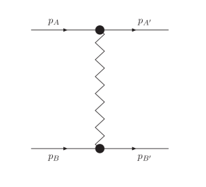
Figure 1: Schematic representation of the process $A+B\rightarrow A^{\prime}+B^{\prime}$ with colour octet in the $t$ channel and negative signature. The zigzag line represents Reggeized gluon.

$${{\cal A}}^{A^{\prime}B^{\prime}}_{AB}={\Gamma}^{c}_{A^{\prime}A}\left[\left({-s\over-t}\right)^{j(t)}-\left({s\over-t}\right)^{j(t)}\right]\Gamma^{c}_{B^{\prime}B}~{},$$ (14)

where ${\Gamma}^{c}_{P^{\prime}P}$ are energy-independent particle-particle-Reggeon (PPR) vertices (or scattering vertices), $c$ is a colour index, $j(t)=1+\omega(t)$ is the Reggeized gluon trajectory.

As it is seen from (14), in the leading order (LO) PPR vertices are determined by the Born amplitudes, so that their calculation is trivial assuming the gluon Reggeization, i.e. the form (14). Expressions for them are also quite simple. In the helicity basis they have the same form for all partons (quarks and gluons in QCD):

$$\Gamma_{P^{\prime}P}^{c}\ =\ gT^{c}_{P^{\prime}P}\delta_{\lambda_{P^{\prime}}\lambda_{P}}\,,$$ (15)

where $T^{c}_{P^{\prime}P}$ are matrix elements of the colour group generators in the corresponding representations and $\lambda$ are parton helicities. Except for a common coefficient the vertices (15) can be written down without calculation, because they are given by forward matrix elements of the conserved current. Note that Eq. (15) implies a definite choice of the relative phase of spin wave functions of particles $P^{\prime}$ and $P$. Evidently, the phase is zero at $t=0$. In (15) the $s$-channel helicity conservation is exhibited explicitly. Note that for gluons and for massive quarks it is valid only in the LO.

Again, as it is seen from (14), the LLA (one-loop) trajectory is determined by the $s$-channel discontinuity of any amplitude. It gives

$$\omega(t)=\frac{g^{2}N_{c}t}{2(2\pi)^{D-1}}\int\!\frac{d^{D-2}q_{1}}{\vec{q}_{1}^{\>2}(\vec{q}-\vec{q}_{1})^{2}}=-g^{2}\frac{N_{c}\Gamma(1-\epsilon)}{(4\pi)^{D/2}}\frac{\Gamma^{2}(\epsilon)}{\Gamma(2\epsilon)}(\vec{q}^{\>2})^{\epsilon}$$

$$\simeq-g^{2}\frac{N_{c}\Gamma(1-\epsilon)}{(4\pi)^{2+\epsilon}}\frac{2}{\epsilon}(\vec{q}^{\>2})^{\epsilon}\,.$$ (16)

In (16) and below the vector sign means transverse to the $p_{A},p_{B}$ plane components, $D=4-2\epsilon$ is the space-time dimension taken different from 4 to regularize infrared divergencies, which are inevitable in parton amplitudes. Of course, using the dimensional regularization in (8) at $m=0$ one obtains $\alpha(t)=1+\omega(t)$, where $\omega(t)$ is given by (16) at $N_{c}=2$.

The Reggeization means also definite (multi-Regge) form of production amplitudes in the multi-Regge kinematics (MRK). MRK is the kinematics where all particles have limited (not growing with $s$) transverse momenta and are combined into jets with limited invariant mass of each jet and large (growing with $s$) invariant masses of any pair of the jets. This kinematics gives dominant contributions to cross sections of QCD processes at high energy $\sqrt{s}$. In each order of perturbation theory dominant (having the largest $\ln s$ degrees) are amplitudes with gluon quantum numbers and a negative signature. For the amplitude ${\cal A}_{2\rightarrow n+2}$ of the process $A+B\rightarrow A^{\prime}+J_{1}+\ldots+J_{n}+B^{\prime}$ of production of $n$ jets with momenta $k_{1},k_{2},\ldots k_{n}$ the MRK means

$$s\gg s_{i}\gg|t_{i}|\simeq\vec{q}^{\;2}_{i},~{}~{}~{}~{}\;\;s\simeq\frac{\prod_{i=1}^{n+1}s_{i}}{\prod_{i=1}^{n}(\vec{k}^{\;2}_{i}+k_{i}^{2})}~{},$$ (17)

where

$$s=(p_{A}+p_{B})^{2},\;s_{i}=(k_{i-1}+k_{i})^{2},\;\;i=1,\cdot\cdot\cdot n+1,\;\;k_{0}\equiv P_{A^{\prime}},\;\;k_{n+1}\equiv P_{B^{\prime}},$$ (18)

$$q_{1}=p_{A}-p_{A}^{\prime},\;q_{j+1}=q_{j}-k_{j},\;j=1,\cdot\cdot\cdot n,\;\;q_{n+1}=p_{B^{\prime}}-p_{B}~{}.$$ (19)

In this region the amplitudes ${\cal A}_{2\rightarrow n+2}$ can be represented by Fig. 2.

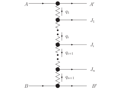
Figure 2: Schematic representation of the process $A+B\rightarrow A^{\prime}+J_{1}+\dots+J_{n}+B^{\prime}$ in MRK. The zig-zag lines represent Reggeized gluon exchange; the black circles denote the Reggeon vertices; $q_{i}$ are Reggeon momenta.

Multi-particle amplitudes have a complicated analytical structure. They are not simple even in MRK (see, for instance, [48] - [32]). Fortunately, only real parts of these amplitudes are used in the BFKL approach in the NLLA as well as in the LLA. The reason is that imaginary parts of amplitudes with negative signature are suppressed by one power of $\ln s$ compared to their real parts, so that account of them in the right part of the unitarity relations (4) means loss of two powers of $\ln s$ (as well as account of amplitudes with positive signature). Restricting ourselves to the real parts we can write

$$\Re{\cal A}_{2\rightarrow n+2}=2s\Gamma^{{R}_{1}}_{A^{\prime}A}\left(\prod_{i=1}^{n}\frac{1}{t_{i}}\Big{(}\frac{s_{i}}{|\vec{k}_{i-1}||\vec{k}_{i}|}\Big{)}^{\omega(t_{i})}\gamma^{G_{i}}_{R_{i}{R}_{i+1}}\right)$$

$$\frac{1}{t_{n+1}}\Big{(}\frac{s_{n+1}}{|k_{n}||\vec{q}_{n+1}|}\Big{)}^{\omega(t_{n+1})}\Gamma^{{R}_{n+1}}_{B^{\prime}B}~{}.$$ (20)

Here ${\Gamma}^{{R}}_{A^{\prime}A}$ and $\Gamma^{{R}}_{B^{\prime}B}$ are the same scattering vertices as in (14) and $\gamma^{J_{i}}_{{R}_{i}{R}_{i+1}}$ are the Reggeon-Reggeon-Jet (RRJ) vertices (or production vertices), i.e. the effective vertices for production of jets $J_{i}$ with momenta $k_{i}$=$q_{i}-q_{i+1}$ in collisions of Reggeons with momenta $q_{i}$ and $-q_{i+1}$.

In the LLA only gluons can be produced, $J=G$,

$$\gamma^{G}_{{R}_{1}{R}_{2}}=gT^{c}_{c_{1}c_{2}}e^{*}_{\mu}(k)C^{\mu}(q_{2},q_{1})\,,$$ (21)

where $k=q_{1}-q_{2}$, $e_{\mu}(k)$ and $c$ are the gluon momentum, polarization vector and colour index, $c_{1}$ and $c_{2}$ are the colour indices of the Reggeons ${R}_{1}$ and ${R}_{1}$ respectively, and $C^{\mu}(q_{1},q_{2})$ is the famous Lipatov’s vertex [1]:

$$C_{\mu}(q_{2},q_{1})\ =\ -q_{1\mu}-q_{2\mu}+p_{1\mu}\left(\frac{q_{1}^{2}}{kp_{1}}+2\frac{kp_{2}}{p_{1}p_{2}}\right)-p_{2\mu}\left(\frac{q_{2}^{2}}{kp_{2}}+2\frac{kp_{1}}{p_{1}p_{2}}\right)$$

$$=\ -q_{1\perp\mu}-q_{2\perp\mu}-\frac{p_{1\mu}}{2(kp_{1})}\left(k_{\perp}^{2}-2q_{1\perp}^{2}\right)+\frac{p_{2\mu}}{2(kp_{2})}\left(k_{\perp}^{2}-2q_{2\perp}^{2}\right).$$ (22)

The Reggeon vertices and the gluon trajectory are known now in the next-to-leading order (NLO), that means the one-loop approximation for the vertices and the two-loop approximation for the trajectory. It is just the accuracy which is required for the derivation of the BFKL equation in the NLLA. Validity of the forms (14) and (20) is proved now in all orders of perturbation theory in the coupling constant $g$ both in the LLA [28] and in the NLLA [51, 52, 53, 54, 55].

In the LLA only gluons can be produced. In the NLA one has to consider not only the amplitudes (14), (20), but also amplitudes obtained from them by replacement of one of final particles by a jet containing a couple of particles with fixed (of order of transverse momenta) invariant mass.

2.2 The scheme of derivation of the BFKL equation

The Reggeization provides a simple derivation of the BFKL equation both in the LLA and NLLA. Two-to-two scattering amplitudes with all possible quantum numbers in the $t$–channel are calculated using the amplitudes   (20) in the $s$-channel unitarity relations (4) and analyticity. The $s$-channel discontinuities of the amplitude ${\cal A}_{AB}^{A^{\prime}B^{\prime}}$ for the high energy process $A+B\rightarrow A^{\prime}+B^{\prime}$ at fixed momentum transfer $\sqrt{-t}$ may be presented by Fig.3,

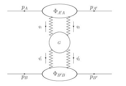
Figure 3: Schematic representation of the $s$-channel discontinuities of amplitudes $A+B\rightarrow A^{\prime}+B^{\prime}$.

where $q_{1}+q_{2}=q^{\prime}_{1}+q^{\prime}_{2}=q=p_{A}-p_{A^{\prime}}=p_{B^{\prime}}-p_{B}$ and symbolically written as the convolution

$$\;\;\;\;\;\;\;\;\Phi_{A^{\prime}A}\;\otimes\;G\;\otimes\;\Phi_{B^{\prime}B}$$

where the impact factors $\Phi_{A^{\prime}A}$ and $\Phi_{B^{\prime}B}$ describe transitions $A\rightarrow A^{\prime}$ and $B\rightarrow B^{\prime}$ due to interactions with Reggeized gluons, $G$ is the Green’s function for two interacting Reggeized gluons with an operator form

$${\hat{\cal G}}=e^{Y\hat{\cal{K}}}~{},$$ (23)

where $\;Y=\ln(s/s_{0})$, $s_{0}$ is an energy scale, ${\hat{\cal{K}}}$ is the BFKL kernel. The impact factors and the BFKL kernel are expressed in terms of the Reggeon vertices and trajectory. Energy dependence of scattering amplitudes is determined by the BFKL kernel, which is universal (process independent). The kernel

$${\hat{\cal{K}}}={\hat{{\omega}_{1}}}+{\hat{{\omega}}_{2}}+{\hat{\cal{K}}_{r}}$$ (24)

is expressed through the Regge trajectories ${\hat{{\omega}}_{1}}$ and ${\hat{{\omega}}_{2}}$ of two gluons and the “real part” ${\hat{\cal{K}}_{r}}$ describing production of particles in their interaction:

$${\hat{\cal{K}}_{r}}={\hat{\cal{K}}_{G}}+{\hat{\cal{K}}_{Q\bar{Q}}}+{\hat{\cal{K}}_{GG}}~{}.$$ (25)

In the LLA only ${\hat{\cal{K}}_{G}}$ must be kept, because only gluons can be produced; in the NLLA production of quark-antiquark (${Q\bar{Q}}$) and gluon ($GG$) pairs is also possible. The impact factors $\Phi_{A^{\prime}A}$ and $\Phi_{B^{\prime}B}$ describing transitions $A\rightarrow A^{\prime}\;\;\;$ and $\;\;\;B\rightarrow B^{\prime}$ depend on properties of scattering particles. All energy dependence is contained in the Green’s function $G$ for two interacting Reggeized gluons.

While the contribution of the trajectories to the kernel is diagonal in colour, the contribution associated with the production of real particles can change colour states. Using the projection operators $\hat{\cal P}^{R}$ on the representation $R$ of the colour group, one can perform the decomposition

$${\hat{\cal{K}}}=\sum_{R}\hat{\cal P}^{R}\hat{\cal{K}}^{R}~{}.$$ (26)

In QCD, possible representations are $\bf{1}$, $\bf{8}_{a}$, $\bf{8}_{s}$, $\bf{10}$, $\bf{10^{*}}$ and $\bf{27}$. In the following, we will consider only the singlet representation, corresponding to scattering of colourless particles, and omit the index $R$.

2.3 Forward BFKL kernel

Separate contributions to the kernel (24) are singular. They were calculated in the dimensional regularization, so that in [46] the kernel also was written at the space-time dimension $D=4-2\epsilon$, different from the physical one. To work with this kernel is rather difficult. But the kernel is infrared safe, i.e. singularities in various parts cancel. It makes possible to perform the cancellation of the most singular terms and to write the kernel in the form [56] (here the Reggeon momenta are q and l )

$${\cal K}(\vec{q},\vec{l})=\frac{\alpha_{s}(\mu^{2})N_{c}}{2\pi^{2}}\left[\frac{2}{(\vec{q}-\vec{l})^{2}}-\delta(\vec{q}-\vec{l})\int\frac{d\vec{k}\;\vec{q}^{\;2}}{(\vec{q}-\vec{k})^{2}\vec{k}^{\>2}}\right]$$

$$\times\left[1+\frac{\alpha_{s}(\mu^{2})N_{c}}{4\pi}\left(\frac{67}{9}-2\zeta(2)-\frac{10}{9}\frac{n_{f}}{N_{c}}\right)\right]$$

$$+\frac{\alpha^{2}_{s}(\mu^{2})N^{2}_{c}}{4\pi^{3}}\left[\frac{1}{(\vec{q}-\vec{l})^{2}}\left(\frac{\beta_{0}}{N_{c}}\ln\left(\frac{{\mu}^{2}}{(\vec{q}-\vec{l})^{\;2}}\right)-\ln^{2}\left(\frac{\vec{q}^{\;{2}}}{\vec{l}^{\;2}}\right)\right)+f_{1}(\vec{q},\vec{l})\right.$$

$$\left.+f_{2}(\vec{q},\vec{l})+\delta(\vec{q}-\vec{l})\left(\frac{\beta_{0}}{2N_{c}}\int\frac{d\vec{k}\;\vec{q}^{\;2}}{(\vec{q}-\vec{k})^{2}\vec{k}^{\>2}}\ln\left(\frac{(\vec{q}-\vec{k})^{2}\vec{k}^{\>2}}{{\mu}^{2}\vec{q}^{\;2}}\right)+6\pi\zeta(3)\right)\right]~{},$$ (27)

where where $\beta_{0}=11N_{c}/3-2n_{f}/3$ is the first coefficient of the $\beta$-function,

$$f_{1}(\vec{q}_{1},\vec{q}_{2})\ =-\ \frac{2(\vec{q}_{1}^{~{}2}-\vec{q}_{2}^{~{}2})}{\vec{k}^{\;2}(\vec{q}_{1}+\vec{q}_{2})^{2}}\Bigg{(}\frac{1}{2}\ln\left(\frac{{\vec{q}_{1}}^{~{}2}}{{\vec{q}_{2}}^{~{}2}}\right)\ln\left(\frac{{\vec{q}_{1}}^{~{}2}{\vec{q}_{2}}^{~{}2}\vec{k}^{\>4}}{\left({\vec{q}^{\;2}_{1}}+{\vec{q}^{\;2}_{2}}\right)^{4}}\right)+Li_{2}\left(-\frac{{\vec{q}_{1}}^{~{}2}}{{\vec{q}_{2}}^{~{}2}}\right)$$

$$-Li_{2}\left(-\frac{{\vec{q}_{2}}^{~{}2}}{{\vec{q}_{1}}^{~{}2}}\right)\Bigg{)}-\left(1-{(\vec{q}_{1}^{~{}2}-\vec{q}_{2}^{~{}2})^{2}}/{\vec{k}^{\>2}(\vec{q}_{1}+\vec{q}_{2})^{2}}\right)\left(\int\limits_{0}^{1}-\int\limits_{1}^{\infty}\right)\frac{dz\,\ln\frac{(z{\vec{q}_{1}})^{2}}{({\vec{q}_{2}})^{2}}}{(\vec{q}_{2}-z\vec{q}_{1})^{2}},$$ (28)

$$f_{2}(\vec{q}_{1},\vec{q}_{2})\ =-\ \left(1+\frac{n_{f}}{N_{c}^{3}}\right)\frac{2{\vec{q}_{1}}^{~{}2}{\vec{q}_{2}}^{~{}2}-3({\vec{q}_{1}}{\vec{q}_{2}})^{2}}{16{\vec{q}_{1}}^{~{}2}{\vec{q}_{2}}^{~{}2}}\left(\frac{2}{{\vec{q}_{2}}^{~{}2}}+\frac{2}{{\vec{q}_{1}}^{~{}2}}+\Big{(}\frac{1}{{\vec{q}_{2}}^{~{}2}}-\frac{1}{{\vec{q}_{1}}^{~{}2}}\Big{)}\ln\frac{{\vec{q}_{1}}^{~{}2}}{{\vec{q}_{2}}^{~{}2}}\right)$$

$$-\ \left(\!3+\Big{(}1+\frac{n_{f}}{N_{c}^{3}}\Big{)}\!\left(\!1-\frac{({\vec{q}_{1}}^{~{}2}+{\vec{q}_{2}}^{~{}2})^{2}}{8{\vec{q}_{1}}^{~{}2}{\vec{q}_{2}}^{~{}2}}-\frac{2{\vec{q}_{1}}^{~{}2}{\vec{q}_{2}}^{~{}2}-3{\vec{q}_{1}}^{~{}4}-3{\vec{q}_{2}}^{~{}4}}{16{\vec{q}_{1}}^{~{}4}{\vec{q}_{2}}^{~{}4}}({\vec{q}_{1}}{\vec{q}_{2}})^{2}\!\right)\!\right)$$

$$\times\ \int\limits_{0}^{\infty}\frac{dx\,\ln\left|\frac{1+x}{1-x}\right|}{{\vec{q}_{1}}^{~{}2}+x^{2}{\vec{q}_{2}}^{~{}2}}~{},$$ (29)

where $\vec{k}=\vec{q}_{1}-\vec{q}_{2}~{}.$

This representation greatly simplifies the calculation of the eigenvalues of the kernel. Strictly speaking, because of the charge renormalization the eigenfunctions of the LO kernel $\left({\vec{l}^{\>2}}\right)^{\gamma-1}$, which at $\gamma=1/2+i\nu,\;\;-\infty<\nu<\infty$ form a complete set for the kernel averaged over angles, are not any more eigenfunctions of the NLO kernel. But with the NLO accuracy one can write

$$\alpha_{s}(\mu^{2})=\alpha_{s}(\vec{q}^{\>2})\left(1+\beta_{0}\frac{\alpha_{s}(\vec{q}^{\>2})}{4\pi}\ln\left(\frac{\vec{q}^{\>2}}{\mu^{2}}\right)\right)~{},$$ (30)

and obtain

$$\int d^{2}l\;{\cal K}(\vec{q},\vec{l})\left(\frac{\vec{l}^{\>2}}{\vec{q}^{\>2}}\right)^{\gamma-1}=\omega(\vec{q}^{\,2},\gamma)=\frac{\alpha_{s}(\vec{q}^{~{}2})\,N_{c}\,}{\pi}\chi(\gamma)~{},\;\;\$$

$$\chi(\gamma)=\chi_{B}(\gamma)+\frac{\alpha_{s}N_{c}}{\pi}\chi^{(1)}(\gamma)~{}.$$ (31)

Here $\chi_{B}(\gamma)$ gives the LO eigenvalues,

$$\chi_{B}(\gamma)=2\psi(1)-\psi(\gamma)-\psi(1-\gamma)$$ (32)

and the correction $\chi^{(1)}(\gamma)$ is:

$$\chi^{(1)}(\gamma)\ =\ -\frac{1}{4}\Bigg{[}\frac{\beta_{0}}{2N_{c}}\left(\chi_{B}^{2}(\gamma)(\gamma)+\chi^{\prime}_{B}(\gamma)-\ 6\zeta(3)\right)$$

$$+\frac{\pi^{2}\cos(\pi\gamma)}{\sin^{2}(\pi\gamma)(1-2\gamma)}\left(3+\left(1+\frac{n_{f}}{N_{c}^{3}}\right)\frac{2+3\gamma(1-\gamma)}{(3-2\gamma)(1+2\gamma)}\right)$$

$$-\ \left(\frac{67}{9}-\frac{\pi^{2}}{3}-\frac{10}{9}\frac{n_{f}}{N_{c}}\right)\chi_{B}(\gamma)+\ \chi_{B}^{\prime\prime}(\gamma))-\frac{\pi^{3}}{\sin(\pi\gamma)}+4\phi(\gamma)\Bigg{]}~{},$$ (33)

where

$$\phi(\gamma)=-\int\limits_{0}^{1}\frac{dx}{1+x}\left(x^{\gamma-1}+x^{-\gamma}\right)\int_{x}^{1}\frac{dt}{t}\ln(1-t)$$

$$=\sum_{n=0}^{\infty}(-1)^{n}\left[\frac{\psi(n+1+\gamma)-\psi(1)}{(n+\gamma)^{2}}+\frac{\psi(n+2-\gamma)-\psi(1)}{(n+1-\gamma)^{2}}\right].$$ (34)

This result was firstly obtained in [46].

The representation (27) is useful also for finding all eigenvalues of the kernel. Defining them as

$$\int d^{2}l\;{K}(\vec{q},\vec{l})\left(\frac{\vec{l}^{\>2}}{\vec{q}^{\>2}}\right)^{\gamma-1}e^{in(\phi_{l}-\phi_{q})}$$

$$=\frac{\alpha_{s}(\vec{q}^{~{}2})\,N_{c}\,}{\pi}\left(\chi_{B}(\gamma,n)+\frac{\alpha_{s}N_{c}}{\pi}\chi^{(1)}(\gamma,n)\right)~{},$$ (35)

where

$$\chi_{B}(\gamma,n)=2\psi(1)-\psi(\gamma+\frac{|n|}{2})-\psi(1-\gamma+\frac{|n|}{2})~{},$$ (36)

we come to the correction obtained in [57]:

$$4\chi^{(1)}\left(\gamma,n\right)\ =\ -\frac{\beta_{0}}{2N_{c}}\left(\chi_{B}^{2}(\gamma,n)+\chi_{B}^{\prime}(\gamma,n)\right)+6\zeta\left(3\right)-\chi_{B}^{\prime\prime}(\gamma,n)$$

$$+\left(\frac{67}{9}-\frac{\pi^{2}}{3}-\frac{10}{9}\frac{n_{f}}{N_{c}}\right)\chi_{B}(\gamma,n)-2\Phi\left(n,\gamma\right)-2\Phi\left(n,1-\gamma\right)+F\left(n,\gamma\right)~{},$$ (37)

where

$$F(n,\gamma)=\frac{\pi^{2}\cos\left(\pi\gamma\right)}{\sin^{2}\left(\pi\gamma\right)\left(1-2\gamma\right)}\Biggl{[}\frac{\gamma\left(1-\gamma\right)\left(\delta_{n,2}+\delta_{n,-2}\right)}{2\left(3-2\gamma\right)\left(1+2\gamma\right)}$$

$$\times\left(1+\frac{n_{f}}{N_{c}^{3}}\right)-\left(\frac{3\gamma\left(1-\gamma\right)+2}{\left(3-2\gamma\right)\left(1+2\gamma\right)}\left(1+\frac{n_{f}}{N_{c}^{3}}\right)+3\right)\delta_{n,0}\Biggr{]}~{},$$ (38)

and

$$\Phi\left(n,\gamma\right)=\int_{0}^{1}\frac{dt}{1+t}t^{\gamma-1+n/2}\left\{\frac{\pi^{2}}{12}-\frac{1}{2}\psi^{\prime}\left(\frac{n+1}{2}\right)-{Li}_{2}\left(t\right)\right.$$

$$-{Li}_{2}\left(-t\right)-\left(\psi\left(n+1\right)-\psi\left(1\right)+\ln\left(1+t\right)+\sum_{k=1}^{\infty}\frac{\left(-t\right)^{k}}{k+n}\right)\ln t$$

$$\left.-\sum_{k=1}^{\infty}\frac{t^{k}}{\left(k+n\right)^{2}}\left[1-\left(-1\right)^{k}\right]\right\}~{}.$$ (39)

3 Investigation of the BFKL properties

In the wide range of problems that Lev dealt with, the BFKL approach was one of the first. Lev many times turned to it, and his analysis was always distinguished by its depth and originality.

3.1 Conformal invariance

In 1985 he discovered that for scattering of colourless particles the LO BFKL equation can be solved in a general form not only for the forward case, but for general momentum transfer [58]. This striking fact is related to the remarkable property of the BFKL equation discovered in [58]: for scattering of colourless particles it can be written in the special representation (which was called later Möbius representation [59]), which is invariant with respect to conformal (Möbius) transformations in the impact parameter space $\vec{r}_{1},\vec{r}_{2}$ of the Reggeized gluons. In this representation the BFKL kernel $\hat{\cal{K}}_{M}$ operates in the space of functions having the colour transparency property (turning into zero at $\vec{r}_{1}=\vec{r}_{2}$). Note that the colourlessness means the Pomeron exchange (while the reverse statement is not correct) and that it is necessary for writing the BFKL equation in the Möbius representation. The colourlessness of colliding particles provides the gauge invariance of impact factors, i.e. their vanishing at zero Reggeized gluon momenta. Together with an analogous property of the BFKL kernel, it gives a possibility to restrict the space of functions where the kernel acts by the functions having the colour transparency.

The conformal invariance of the BFKL equation in the Möbius representation is extremely important because it permits to classify all solutions of the homogeneous equation and to find their complete set. Another significant property is the holomorphic separability of BFKL kernel in this representation. Actually, this property was used already in [58]; it was explicitly exhibited and used later [60, 61] for solving the Bartels-Kwiecinski-Praszalowichz (BKP) equation – the generalization of the BFKL equation to the case of many Reggeized gluons in the $t$–channel [50, 62]. The conformal invariance permits to obtain eigenfunctions of the kernel $\hat{\cal{K}}_{M}$ from eigenfunctions for forward scattering by transformations of the Möbius group (inversion and shift). In [58] they were chosen in the form

$$E_{n,\nu}(\vec{r}_{10},\vec{r}_{20})=(-1)^{n}\left(\frac{z_{12}}{z_{10}z_{20}}\right)^{\frac{1}{2}+i\nu-\frac{n}{2}}\left(\frac{z^{*}_{12}}{z^{*}_{10}z^{*}_{20}}\right)^{\frac{1}{2}+i\nu+\frac{n}{2}}~{},$$ (40)

where $z=x+iy$ for $\vec{r}=(x,y)$, the vector $\vec{r}_{0}$ is introduced for indexing of the wave functions, $\vec{r}_{ij}=\vec{r}_{i}-\vec{r}_{j}$, $n$ is integer and $\nu$ is real. The eigenvalues coincide with the eigenvalues of the forward kernel

$$\omega_{B}(\gamma,n)=\frac{\alpha_{s}N_{c}}{\pi}\chi_{B}(\gamma,n)~{},\gamma=1/2+i\nu~{},$$ (41)

$\chi_{B}(\gamma,n)$ is given in (36). One can see it noticing that the eigenvalues do not depend on $\vec{r}_{0}$ and that integration over $\vec{r}_{0}$ gives

$$\int\,d\vec{r}_{0}\,E_{n,\nu}(\vec{r}_{10},\vec{r}_{20})=C_{n,\nu}\,(z_{12})^{\frac{1}{2}-i\nu+\frac{n}{2}}(z^{*}_{12})^{\frac{1}{2}-i\nu-\frac{n}{2}}=C_{n,\nu}\,e^{i\,n\phi_{12}}\vec{r}_{12}^{2(1-\gamma)}~{},$$ (42)

where $\phi_{12}$ is the azimuthal angle of the vector $\vec{r}_{12}$. Then the problem is reduced to the calculations of the integrals for the forward case. The form of the integral (42) can be easily obtained using the change of the integration variables $z_{10}=z_{12}z$; the coefficient $C_{n,\nu}$ is irrelevant for the calculation of the eigenvalues. In fact, it was found in [58]:

$$C_{n,\nu}=\frac{\pi 2^{4\,i\,\nu}}{|n|-2\,i\,\nu}\frac{\Gamma(\kappa)}{\Gamma(\kappa^{*})}\frac{\Gamma(\kappa^{*}-1/2)}{\Gamma(\kappa-1/2)}~{},\;\;\kappa=\frac{1}{2}-i\nu+\frac{|n|}{2}~{}.$$ (43)

One can easily show that

$$z^{2}_{12}\frac{\partial}{\partial z_{1}}\frac{\partial}{\partial z_{2}}\,E_{n,\nu}=\lambda_{n,\nu}E_{n,\nu}~{},\;\;z^{*\,2}_{12}\frac{\partial}{\partial z^{*}_{1}}\frac{\partial}{\partial z^{*}_{2}}\,E_{n,\nu}=\lambda_{n,-\nu}E_{n,\nu}~{},$$

$$\lambda_{n,\nu}=\frac{1}{4}-(\frac{n}{2}-i\nu)^{2}~{}.$$ (44)

The completeness condition derived in [58] has the form

$$4\sum_{n=-\infty}^{+\infty}\int_{-\infty}^{+\infty}\ d\nu\int\ d^{2}r_{0}\frac{n^{2}+4\nu^{2}}{\vec{r}^{2}_{12}\vec{r}^{2}_{1^{\prime}2^{\prime}}}E_{n,\nu}(\vec{r}_{10},\vec{r}_{20})E^{*}_{n,\nu}(\vec{r}_{1^{\prime}0},\vec{r}_{2^{\prime}0})$$

$$=(2\pi)^{4}\delta(\vec{r}_{11^{\prime}})\delta(\vec{r}_{22^{\prime}})~{}.$$ (45)

Using (44) and (45) one obtains for the Green’s function in the impact parameter space

$$\langle\vec{r}_{1},\vec{r}_{2}|\frac{1}{\omega-\hat{\cal{K}}_{M}}\frac{1}{\hat{\vec{q}}_{\,1}^{\,2}\hat{\vec{q}}_{\,2}^{\,2}}|\vec{r}_{\,1}^{\;\prime},\vec{r}_{\,2}^{\;\prime}\rangle$$

$$=4\sum_{n=-\infty}^{+\infty}\int_{-\infty}^{+\infty}\ d\nu\int\ d^{2}r_{0}\frac{({n^{2}+4\nu^{2}})E_{n,\nu}(\vec{r}_{10},\vec{r}_{20})E^{*}_{n,\nu}(\vec{r}_{1^{\prime}0},\vec{r}_{2^{\prime}0})}{[(n+1)^{2}+4\nu^{2}][(n-1)^{2}+4\nu^{2}](\omega-\omega(\gamma,n))}~{}.$$ (46)

For $n=\pm 1$ the integral over $\nu$ here must be taken in the sense of its principal value.

Later an explicit expression for the kernel ${\cal{K}_{M}}$ in the impact parameter space was obtained [63]:

$$\langle\vec{r}_{1},\vec{r}_{2}|\hat{\cal{K}}_{M}|\vec{r}_{1}^{\;\prime},\vec{r}_{2}^{\;\prime}\rangle$$

$$=\frac{\alpha_{s}N_{c}}{2\pi^{2}}\int\,{d\vec{r}_{0}}\ \frac{\vec{r}_{12}^{\,2}}{\vec{r}_{10}^{\,2}\vec{r}_{20}^{\;2}}\left(\delta(\vec{r}_{11^{\prime}})\delta(\vec{r}_{02^{\prime}})+\delta(\vec{r}_{22^{\prime}})\delta(\vec{r}_{01^{\prime}})-\delta(\vec{r}_{11^{\prime}})\delta(\vec{r}_{22^{\prime}})\right)~{},$$ (47)

where the subscript $M$ denotes the Möbius form. It is worth to note that the ultraviolet singularities of separate terms in (47) cancel in their sum with account of the dipole property of the target impact factors.

The transformations of the Möbius group in the two-dimensional space $\vec{r}=(x,y)$ can be written as

$$z\rightarrow\frac{az+b}{cz+d}\;,\;\;\;$$ (48)

where $z=x+iy,\;\;a,b,c,d$ are complex numbers, with $ad-bc\neq 0$. Under these transformations, one has

$$z_{1}-z_{2}\rightarrow\frac{z_{1}-z_{2}}{(cz_{1}+d)(cz_{2}+d)}(ad-bc)\;,$$

$$dzdz^{*}\rightarrow dzdz^{*}\frac{|ad-bc|^{2}}{\left|(cz+d)^{2}\right|^{2}}\;,$$ (49)

so that the conformal invariance of (47) is evident.

It turns out that the Möbius form (47) coincides with the kernel of the colour dipole model [64]-[67] formulated in the coordinate space. It means that the colour dipole kernel could have been written by Lev as early as 1985. It was not done only by chance, because he used the operator form of the kernel instead of the explicit expression for it in the impact parameter space.

Investigation of the conformal properties of the BFKL kernel in the NLO [68] - [71] showed later that the ambiguity of the NLO kernel allows to present the kernel in the form where the conformal invariance is violated only by renormalization.

In the same paper [58] Lev performed another great study: account of running of the coupling constant. Strictly speaking, this account oversteps the limits of the LLA. Nevertheless, it is not unreasonable to take it into account just in the LO BFKL kernel in order to understand qualitative effects of the running. One important effect discovered by Lev is the conversion of the cut $[0,\omega_{P}^{B}]$ into an infinite series of moving poles with limiting point at $\omega=0$. The Pomeron trajectories found in [58] are represented in the form

$$\omega_{k}(t)=\frac{c}{k+\eta(q^{2})+1/4}~{},\;\;k=0,\,\pm 1,\,\pm 2\,...,$$ (50)

where $c$ is a calculable constant. The function $\eta(q^{2})$ is determined by large distances, but is limited by the inequalities $-1\leq 4\eta\leq 1$ at small $|t|$. In the region of large $|t|$ ($\alpha_{s}(|t|)\ll 1$) the family of poles is approximated by the moving cut with the branch point

$$\omega(t)=\frac{4N_{c}}{\pi}\ln 2\,\,\alpha_{s}(|t|)~{}.$$ (51)

3.2 Relation with DGLAP

The relation between the eigenvalues of BFKL kernel $\frac{\alpha_{s}N_{c}}{\pi}\chi(\gamma)$ and the anomalous dimension $\gamma_{\omega}$ of the twist-2 operators with $j=1+\omega$ was first discovered in the LLA in [72], where it has the form:

$$\omega=\frac{\alpha_{s}N_{c}}{\pi}\chi(\gamma_{\omega})~{}.$$ (52)

It is a remarkable result because it means that the BFKL approach permits to obtain the resummation of the most singular at $j=1$ terms in the anomalous dimension of the twist-two operators.

It was noticed in [46] that in the NLLA this relation must be changed. The reason is that energy scale $s_{0}$ becomes significant in the NNLLA, and this scale is different from DGLAP. In the NLA $s_{0}=Q_{A}Q_{B}$, where $Q_{A}$ and $Q_{B}$ are typical momenta for the impact factors $\Phi_{A}$ and $\Phi_{B}$. Therefore the deep-inelastic moments are defined as

$$M_{\omega}(Q^{2})\ =\ \frac{1}{4(2\pi)^{2}}\int\frac{d\vec{q}}{\vec{q}^{2}}\int\frac{d\vec{l}}{\vec{l}^{2}}\Phi_{A}(\vec{q})e^{\omega\ln(Q/Q_{B})}G_{\omega}(\vec{q},\vec{l})\Phi_{B}(\vec{l})\,.$$ (53)

As the result, for the anomalous dimension $\gamma_{\omega}(\alpha_{s})$ one has

$$\gamma_{\omega}=\frac{\omega}{2}+\chi^{-1}\left(\frac{\pi\omega}{N_{c}\alpha_{s}}\right)~{},$$ (54)

where $\chi^{-1}$ is the inverse function. In other words, the anomalous dimensions $\gamma_{\omega}(\alpha_{s})$ of the twist-2 operators near the point $\omega=0$ are determined from the solution of the equation

$$\omega\ =\ \frac{\alpha_{s}N_{c}}{\pi}\chi(\gamma-\frac{\omega}{2})\simeq\frac{\alpha_{s}N_{c}}{\pi}\chi(\gamma)-\frac{\alpha^{2}_{s}N^{2}_{c}}{2\pi^{2}}\chi(\gamma)\chi^{\prime}(\gamma)$$

$$\simeq\frac{\alpha_{s}N_{c}}{\pi}\frac{1}{\gamma}-\frac{\alpha_{s}^{2}N_{c}^{2}}{4\,\pi^{2}}\left(\frac{11+2n_{f}/N_{c}^{3}}{3\,\gamma^{2}}+\ \frac{n_{f}(10+13/N_{c}^{2})}{9\gamma\,N_{c}}\right.$$

$$\left.+\frac{395}{27}-2\zeta(3)-\frac{11}{3}\frac{\pi^{2}}{6}+\frac{n_{f}}{N_{c}^{3}}\left(\frac{71}{27}-\frac{\pi^{2}}{9}\right)+{\cal O}(\gamma)\right)$$ (55)

for $\gamma\rightarrow 0$. This equation was derived in [46] and used to reproduce the known results and predict the higher loop correction for $\omega\rightarrow 0$:

$$\gamma \simeq \frac{\alpha_{s}\,N_{c}}{\pi}\left(\frac{1}{\omega}-\frac{11}{12}-\frac{n_{f}}{6N_{c}^{3}}\right)-\left(\frac{\alpha_{s}\,}{\pi}\right)^{2}\frac{n_{f}\,N_{c}}{6\,\omega}\left(\frac{5}{3}+\frac{13}{6N_{c}^{2}}\right)$$ (56)

$$-\ \frac{1}{4\omega^{2}}\left(\frac{\alpha_{s}N_{c}}{\pi}\right)^{3}\left(\frac{395}{27}-2\zeta(3)-\frac{11}{3}\frac{\pi^{2}}{6}+\frac{n_{f}}{N_{c}^{3}}\left(\frac{71}{27}-\frac{\pi^{2}}{9}\right)\right).$$

The result for the three-loop correction was confirmed later in [73], [74].

3.3 BFKL in N=4 SUSY

Impressive and surprising results connected with BFKL were obtained by Lev in maximally extended supersymmetric Yang-Mills theory (N=4 SYM). The eigenvalues of the NLO BFKL kernel were calculated in [57]. They turned out to be much simpler than in QCD: instead of (37) the one-loop correction takes the form

$$4\chi^{(1)}\left(\gamma,n\right)\ =-2\Phi\left(n,\gamma\right)-2\Phi\left(n,1-\gamma\right)+6\zeta(3)+\psi^{\prime\prime}(\gamma+\frac{n}{2})+\psi^{\prime\prime}(\gamma+\frac{n}{2})~{}.$$ (57)

A remarkable fact is the disappearance of non analytical in conformal spin $n$ terms. Moreover, all functions entering in (57) have the property of maximal transcendentality [74]. The maximal transcendentality of an expression means by definition, that the special functions and numbers with lower complexities do not contribute to it. By definition $\psi(x)$ has the transcendentality equal to 1, the transcendentalities of $\psi^{(n)}$ and $\zeta(n+1)$ are $n+1$ and the additional poles in the sum over $k$ increase the transcendentality of the function $\Phi(M)$ up to 3. Lev put forward a remarkable hypothesis about growing with order of perturbation theory maximal transcendentality of the eigenvalues of the BFKL kernel and the anomalous dimensions of twist-2 operators in $N=4$ SUSY. This hypothesis is not disproved and widely used now. Another of Lev’s remarkable hypothesis is the hypothesis that in $N=4$ SUSY the Pomeron coincides with the Reggeized graviton, which gives a possibility to calculate its intercept at large coupling constants. Maximal transcendentality together with integrability allow one to find the anomalous dimensions of twist-2 operators in this model up to 4 loops.

4 Future development

Evidently, the next step in the development of the BFKL approach should be the next-to-next-to-leading logarithmic approximation (NNLLA). Unfortunately, in QCD the BFKL equation in the next-to-next-to-leading approximation is not yet obtained, although in maximally extended supersymmetric Yang-Mills theory with large number of colours (planar N=4 SYM) impressive results have been obtained [75] - [78].

4.1 NNLLA BFKL in planar N=4 SYM

In [75] the next-to-next-to-leading order (NNLO) corrections to the BFKL Pomeron eigenvalues for conformal spin $n=0$ were obtained. The method of calculation was quite different from the one used in the BFKL approach, in which, first of all, the kernel of the BFKL equation is calculated using the unitarity and analyticity. It was based on the integrability of the planar N=4 SYM and on the observation of L. N. Lipatov and A.V. Kotikov [57] that BFKL eigenvalues and anomalous dimensions of twist-2 operators are connected in planar N=4 SYM by analytic continuation. The problem of calculation of the anomalous dimensions was solved by the quantum spectral curve method (QSC) [79], [80] giving a finite set of Riemann-Hilbert equations for exact spectrum of planar N=4 SYM theory. Applicability of this method to calculation of the LO BFKL Pomeron eigenvalues was demonstrated in [81]. Another significant assumption, besides the applicability of the QSC, was the possibility to write the relation between the spin $S$ of the twist-two operator $Tr(ZD_{+}^{S}Z)$ and its full conformal dimension $\Delta=2+S+\gamma$, $\gamma$ is the anomalous dimension, in the form

$$j(\Delta)=2+S(\Delta)=1+\sum\limits_{n=1}^{\infty}(\frac{g^{2}N_{c}}{(4\pi)^{2}})^{n}\left[F_{n}\left(\frac{\Delta-1}{2}\right)+F_{n}\left(\frac{-\Delta-1}{2}\right)\right]~{},$$ (58)

where $F_{n}(x)$ are simple linear combinations of the nested harmonic sums with the same transcendentality $n$

$$S_{a_{1},a_{2},\dots,a_{n}}(x)=\sum\limits_{y=1}^{x}\frac{(\textrm{sign}\left(a_{1}\right))^{y}}{y^{|a_{1}|}}S_{a_{2},\dots,a_{n}}(y)\;\;,\;\;S(x)=1\;.$$ (59)

The possibility of such representation for the LO and NLO eigenvalues with

$$F_{1}=-4S_{1},\frac{F_{2}}{4}=-\frac{3}{2}\zeta_{3}+\pi^{2}\ln 2+\frac{\pi^{2}}{3}S_{1}+2S_{3}+\pi^{2}S_{-1}-4S_{-2,1}$$ (60)

was shown in [82]. The three-loop result obtained in [75] is:

$$\frac{F_{3}(x)}{256}=-\frac{5S_{-5}}{8}-\frac{S_{-4,1}}{2}+\frac{S_{1}S_{-3,1}}{2}+\frac{S_{-3,2}}{2}-\frac{5S_{2}S_{-2,1}}{4}+\frac{S_{-4}S_{1}}{4}+\frac{S_{-3}S_{2}}{8}$$

$$+\frac{3S_{3,-2}}{4}-\frac{3S_{-3,1,1}}{2}-S_{1}S_{-2,1,1}+S_{2,-2,1}+3S_{-2,1,1,1}-\frac{3S_{-2}S_{3}}{4}-\frac{S_{5}}{8}$$

$$+\frac{S_{-2}S_{1}S_{2}}{4}+\pi^{2}\left[\frac{S_{-2,1}}{8}-\frac{7S_{-3}}{48}-\frac{S_{-2}S_{1}}{12}+\frac{S_{1}S_{2}}{48}\right]\!-\!\pi^{4}\left[\frac{2S_{-1}}{45}-\frac{S_{1}}{96}\right]$$

$$+\zeta_{3}\left[-\frac{7S_{-1,1}}{4}+\frac{7S_{-2}}{8}+\frac{7S_{-1}S_{1}}{4}-\frac{S_{2}}{16}\right]$$

$$+\left[2\text{Li}_{4}\!\!\left(\tfrac{1}{2}\right)-\frac{\pi^{2}\log^{2}\!2}{12}+\frac{\log^{4}\!2}{12}\right]\left(S_{-1}-S_{1}\right)$$

$$+\frac{\log^{5}\!2}{60}-\frac{\pi^{2}\log^{3}\!2}{36}-\frac{2\pi^{4}\log 2}{45}-\frac{\pi^{2}\zeta_{3}}{24}+\frac{49\zeta_{5}}{32}-2\text{Li}_{5}\!\!\left(\tfrac{1}{2}\right)\;.$$ (61)

The eigenvalues $\omega(\gamma)=j(i\nu)-1$ at $\gamma=\frac{1}{2}+i\nu$ correspond to complex values of $\Delta$ and require analytical continuation of the harmonic sums. Corresponding prescriptions can be found in [83] -[86].

The approach used in [76] was also different from the BFKL approach. The NNLO corrections to the Pomeron eigenvalues for conformal spin $n=0$ were obtained from the constraints, coming from the six-loop anomalous dimension of twist-2 operators and large-gamma limit. The results agree with [75].

The calculations of the three-loop corrections in [77] is closer to the BFKL approach since the corrections are calculated firstly to the BFKL kernel (in the Pomeron channel). But the method of the calculation is quite different from the dispersive method used in the BFKL approach. Moreover, the kernel is calculated not in the momentum representation, but in the impact parameter space. The method used is based on established in [87] connection of the BFKL logarithms with so-called non-global logarithms [88], [89] the physics of soft wide-angle radiation.

In [78] a general non-perturbative framework for the BFKL spectrum of planar N = 4 SYM was developed. As well as in [75], it is based on the QSC method, but the spectrum was studied at arbitrary values of conformal spin n.

4.2 NNLLA in the BFKL approach

The results described above were obtained in $N=4$ SUSY model with unique properties and concern only the BFKL kernel. Recall that amplitudes are given by convolution of impact factors of scattering particles and the Green’s function, which is determined by the kernel, so that to calculate the amplitudes, it is necessary to know not only the kernel, but also the impact factors. The BFKL approach gives an algorithm for calculating both components. Besides this, the amplitudes of both elastic and inelastic processes are calculated in the original (dispersive) BFKL approach. Therefore, its development in the NNLLA is very desirable. And finally, it is highly desirable to develop this approach in QCD. Unfortunately, this development is facing great difficulties.

Remind that original scheme of derivation of the BFKL equation looks as follows. Elastic scattering amplitudes are calculated using the $s$-channel unitarity and analyticity. In the LLA and in the NLLA, only amplitudes having the pole Regge form contribute to unitarity relations. It permits to present the $s$-channel discontinuities of elastic processes as the convolutions of impact factors of scattering particles and the Green’s function for two interacting Reggeized gluons. All these components are expressed in terms of the Reggeon vertices and trajectory.

If this scheme were applicable, for derivation of the BFKL equation in the NNLLA would be sufficient to calculate three-loop corrections to the trajectory, two-loop corrections to the vertex of one gluon production, one-loop corrections to the vertices of two gluon and quark-antiquark production and to find in the Born approximation new vertices: for three gluon and quark-antiquark-gluon production.

However, this scheme is based on the pole Regge form of amplitudes which are used in the unitarity relations (4). It can not be used the NNLLA. In this approximation two large logarithms can be lost in the product of two amplitudes in the unitarity relations (4). It can be done losing either one logarithm in each of the amplitudes or both logarithms in one of the amplitudes.

In the first case it becomes necessary to take into account the imaginary parts of amplitudes with negative signature as well as amplitudes with positive signature, which both are suppressed by one degree of the logarithm. Note that the simple factorized form (20) is valid only for the real part of the amplitudes and must be corrected to account for the imaginary parts, which creates certain difficulties. But more difficulties are connected with the second case. In this case one of the amplitudes in (4) must be taken in the LLA and the other in the NNLLA. Since the amplitudes in the LLA are real, only real parts of the NNLLA amplitudes are important in this case. But even for these parts the pole Regge form becomes inapplicable because of the contributions of the three-Reggeon cuts which appear in this approximation.

The first observation of the violation the pole Regge form was done [90] in the high-energy limit of the results of direct two-loop calculations of the two-loop amplitudes for $gg,gq$ and $qq$ scattering. Then, the terms breaking the pole Regge form in two and three-loop amplitudes of elastic scattering were found in [91, 92, 93] using the techniques of infrared factorization.

It is necessary to say that, in general, breaking of the pole Regge form is not a surprise. It is well known that Regge poles in the complex angular momenta plane generate Regge cuts. Moreover, in amplitudes with positive signature the Regge cuts appear already in the LLA. In particular, the BFKL Pomeron is the two-Reggeon cut in the complex angular momentum plane. But in amplitudes with negative signature Regge cuts appear only in the NNLLA. It is natural to expect that the observed violation of the pole Regge form can be explained by their contributions.

Indeed, all known cases of breaking of the pole Regge form are now explained by the three-reggeon cuts [94, 95]. Unfortunately, the approaches and the explanations used in these papers are different. Their results coincide in three loops but may diverge in more loops. It requires further investigation.

Consideration of three-reggeon cuts in many-particle amplitudes is an even more complicated problem.

5 Conclusion

L.N. Lipatov stood at the origins of the BFKL approach and played a prominent role in its development. He left a huge legacy to his disciples and followers. Unfortunately, now they are deprived of his highest skill, and the depth and originality of his ideas.

References

- [1] L. N. Lipatov, Sov. J. Nucl. Phys. 23 (1976) 338 [Yad. Fiz. 23 (1976) 642].
- [2] C. N. Yang and R. L. Mills, Phys. Rev. 96 (1954) 191.
- [3] P. W. Higgs, Phys. Rev. 145 (1966) 1156.
- [4] T. W. B. Kibble, Phys. Rev. 155 (1967) 1554.
- [5] F. Englert and R. Brout, Phys. Rev. Lett. 13 (1964) 321.
- [6] M. Gell-Mann and M. L. Goldberger, Phys. Rev. Lett. 9 (1962) no.6, 275.
- [7] M. Gell-Mann, M. L. Goldberger, F. E. Low and F. Zachariasen, Phys. Lett. 4 (1963) no.5, 265.
- [8] M. Gell-Mann, M. Goldberger, F. Low, E. Marx and F. Zachariasen, Phys. Rev. 133 (1964) no.1B, B145.
- [9] M. Gell-Mann, M. L. Goldberger, F. E. Low, V. Singh and F. Zachariasen, Phys. Rev. 133 (1964) B161.
- [10] S. Mandelstam, Phys. Rev. 137 (1965) B949.
- [11] S. Mandelstam, Conference: C64-08-05, p.376-377. Proceedings, 12th International Conference on High Energy Physics (ICHEP 1964) : Dubna, 1964.
- [12] A.N. Chester, Phys. Rev. B 140 (1965) B85.
- [13] H. Cheng and C. C. Lo, Phys. Lett. 57B (1975) 177.
- [14] E. Abers, R. A. Keller and V. L. Teplitz, Phys. Rev. D 2 (1970) 1757.
- [15] D. A. Dicus, D. Z. Freedman and V. L. Teplitz, Phys. Rev. D 4 (1971) 2320.
- [16] M. T. Grisaru, H. J. Schnitzer and H. S. Tsao, Phys. Rev. Lett. 30 (1973) 811;
- [17] M. T. Grisaru, H. J. Schnitzer and H. S. Tsao, Phys. Rev. D 8 (1973) 4498.
- [18] M. T. Grisaru, Phys. Rev. D 16 (1977) 1962.
- [19] V. N. Gribov, Sov. Phys. JETP 14 (1962) 1395 [ Zh. Eksp. Teor. Fiz. 41 (1961) 1962].
- [20] Chew, G. F. and Frautschi, S. C., Phys. Rev. Lett. 7 (1961) 394.
- [21] V. N. Gribov, L. N. Lipatov and G. V. Frolov, Sov. J. Nucl. Phys. 12 (1971) 543 [Yad. Fiz. 12 (1970) 994].
- [22] G. V. Frolov, V. N. Gribov and L. N. Lipatov, Phys. Lett. 31B (1970) 34.
- [23] H. Cheng and T. T. Wu, Phys. Rev. D1 (1970) 2775.
- [24] Froissart, M., Phys. Rev. 123 (1961) 1053.
- [25] V.S. Fadin, E.A. Kuraev, and L.N. Lipatov, Phys. Lett. B 60 (1975) 50-52.
- [26] E.A. Kuraev, L.N. Lipatov, and V.S. Fadin, Zh. Eksp. Teor. Fiz. 71 (1976) 840-855 [Sov. Phys. JETP 44 (1976) 443-450].
- [27] E.A. Kuraev, L.N. Lipatov, and V.S. Fadin, Zh. Eksp. Teor. Fiz. 72 (1977) 377-389 [Sov. Phys. JETP 45 (1977) 199-207].
- [28] Ya.Ya. Balitskii, L.N. Lipatov, and V.S. Fadin,“Regge Processes In Nonabelian Gauge Theories” (in Russian), in Materials of IV Winter School of LNPI (Leningrad, 1979), pp. 109-149.
- [29] I.I. Balitsky, and L.N. Lipatov, Yad. Fiz. 28 (1978) 1597-1611 [Sov. J. Nucl. Phys. 28 (1978) 822-829].
- [30] V. S. Fadin and L. N. Lipatov, JETP Lett. 49 (1989) 352 [Yad. Fiz. 50 (1989) 1141] [Sov. J. Nucl. Phys. 50 (1989) 712].
- [31] V. S. Fadin and R. Fiore, Phys. Lett. B 294 (1992) 286.
- [32] V. S. Fadin and L. N. Lipatov, Nucl. Phys. B 406 (1993) 259.
- [33] V. S. Fadin, R. Fiore and A. Quartarolo, Phys. Rev. D 50 (1994) 2265.
- [34] V. S. Fadin, R. Fiore and A. Quartarolo, Phys. Rev. D 50 (1994) 5893.
- [35] V. S. Fadin, Phys. Atom. Nucl. 58 (1995) 1762 [Yad. Fiz. 58 (1995) 1839].
- [36] V. S. Fadin, JETP Lett. 61 (1995) 346 [Pisma Zh. Eksp. Teor. Fiz. 61 (1995) 342].
- [37] V. S. Fadin, M. I. Kotsky and R. Fiore, Phys. Lett. B 359 (1995) 181.
- [38] V. S. Fadin,
- [39] V. S. Fadin, R. Fiore and A. Quartarolo, Phys. Rev. D 53 (1996) 2729
- [40] V. S. Fadin and L. N. Lipatov, Nucl. Phys. B 477 (1996) 767
- [41] M. I. Kotsky and V. S. Fadin, Phys. Atom. Nucl. 59 (1996) 1035 [Yad. Fiz. 59N6 (1996) 1080].
- [42] V. S. Fadin, R. Fiore and M. I. Kotsky, Phys. Lett. B 387 (1996) 593
- [43] V. S. Fadin, M. I. Kotsky and L. N. Lipatov, hep-ph/9704267.
- [44] V. S. Fadin, M. I. Kotsky and L. N. Lipatov, Phys. Lett. B 415 (1997) 97.
- [45] V. S. Fadin, R. Fiore, A. Flachi and M. I. Kotsky, Phys. Lett. B 422 (1998) 287.
- [46] V. S. Fadin and L. N. Lipatov, Phys. Lett. B 429 (1998) 127.
- [47] M. Ciafaloni and G. Camici, Phys. Lett. B 430 (1998) 349.
- [48] J. Bartels, Phys. Rev. D11 (1975) 2977.
- [49] J. Bartels, Phys. Rev. D11 (1975) 2989.
- [50] J. Bartels, Nucl. Phys. B175 (1980) 365.
- [51] V.S. Fadin, R. Fiore, M.G. Kozlov, and A.V. Reznichenko, Phys. Lett. B 639, 74-81 (2006).
- [52] M.G. Kozlov, A.V. Reznichenko, and V.S. Fadin, Yad. Fiz. 74, 784-796 (2011) [Phys. Atom. Nucl. 74, 758-770 (2011)].
- [53] M.G. Kozlov, A.V. Reznichenko, and V.S. Fadin, Yad. Fiz. 75, 905-920 (2012) [Phys. Atom. Nucl. 75, 850-863 (2012)].
- [54] M.G. Kozlov, A.V. Reznichenko, and V.S. Fadin, Yad. Fiz. 75, 529-542 (2012) [Phys. Atom. Nucl. 75, 493-506 (2012).
- [55] V. S. Fadin, M. G. Kozlov, and A. V. Reznichenko, Phys. Rev. D 92 no.8, 085044 (2015).
- [56] V. S. Fadin, R. Fiore and A. V. Grabovsky, Nucl. Phys. B 820 (2009) 334.
- [57] A. V. Kotikov and L. N. Lipatov, Nucl. Phys. B 582 (2000) 19.
- [58] L. N. Lipatov, Sov. Phys. JETP 63 (1986) 904 [Zh. Eksp. Teor. Fiz. 90 (1986) 1536].
- [59] J. Bartels, L.N. Lipatov and G.P. Vacca, Nucl. Phys. B706 (2005) 391.
- [60] L. N. Lipatov, Phys. Lett. B 251 (1990) 284.
- [61] L. N. Lipatov, Phys. Lett. B 309 (1993) 394.
- [62] J. Kwiecinski and M. Praszalowicz, Phys. Lett. B 94 (1980) 413.
- [63] V. S. Fadin, R. Fiore and A. Papa, Nucl. Phys. B 769 (2007) 108
- [64] N.N. Nikolaev and B.G. Zakharov, Z. Phys. C64 (1994) 631.
- [65] N.N. Nikolaev, B.G. Zakharov, and V.R. Zoller, JETP Lett. 59 (1994) 6.
- [66] A.H. Mueller, Nucl. Phys.B415 (1994) 373.
- [67] A.H. Mueller and B. Patel, Nucl. Phys. B425 (1994) 471.
- [68] V. S. Fadin, R. Fiore, and A. Papa, Phys. Lett. B647 (2007) 179.
- [69] V. S. Fadin, R. Fiore, A. V. Grabovsky, and A. Papa, Nucl. Phys. B784, 49 (2007).
- [70] V. S. Fadin and R. Fiore, Phys. Lett. B661 (2008) 139.
- [71] V. S. Fadin, R. Fiore and A. V. Grabovsky, Nucl. Phys. B 831 (2010) 248.
- [72] Jaroszewicz, T., Phys. Lett. B116 (1982) 291.
- [73] Vogt, A., Moch, S. and Vermaseren, J. A. M., Nucl. Phys. B691 (2004) 129.
- [74] A. V. Kotikov, L. N. Lipatov, A. I. Onishchenko and V. N. Velizhanin, Phys. Lett. B 595 (2004) 521 Erratum: [Phys. Lett. B 632 (2006) 754]
- [75] N. Gromov, F. Levkovich-Maslyuk and G. Sizov, Phys. Rev. Lett. 115 (2015) no.25, 251601.
- [76] V. N. Velizhanin, arXiv:1508.02857 [hep-th].
- [77] S. Caron-Huot and M. Herranen, JHEP 1802 (2018) 058.
- [78] M. Alfimov, N. Gromov and G. Sizov, JHEP 1807 (2018) 181.
- [79] N. Gromov, V. Kazakov, S. Leurent and D. Volin, Phys. Rev. Lett. 112 (2014) no.1, 011602.
- [80] N. Gromov, V. Kazakov, S. Leurent and D. Volin, JHEP 1509 (2015) 187.
- [81] M. Alfimov, N. Gromov and V. Kazakov, JHEP 1507 (2015) 164.
- [82] M. S. Costa, V. Goncalves and J. Penedones, “Conformal Regge theory,” JHEP 1212 (2012) 091.
- [83] A. V. Kotikov and V. N. Velizhanin, hep-ph/0501274.
- [84] D. I. Kazakov and A. V. Kotikov, Nucl. Phys. B 307 (1988) 721 Erratum: [Nucl. Phys. B 345 (1990) 299].
- [85] C. Lopez and F. J. Yndurain, Nucl. Phys. B 183 (1981) 157.
- [86] J. Blumlein, Comput. Phys. Commun. 180 (2009) 2218
- [87] S. Caron-Huot, JHEP 1803 (2018) 036
- [88] M. Dasgupta and G. P. Salam, Phys. Lett. B 512 (2001) 323
- [89] A. Banfi, G. Marchesini and G. Smye, JHEP 0208, 006 (2002).
- [90] Del Duca V., Glover E.W.N., JHEP. 0110 (2001) 035.
- [91] Del Duca V., Falcioni G., Magnea L., Vernazza L. Phys. Lett. B. 732 (2014) 233
- [92] Del Duca V., Falcioni G., Magnea L., Vernazza L., PoS RADCOR 2013 (2013) 046.
- [93] Del Duca V., Falcioni G., Magnea L., Vernazza L., JHEP 1502 (2015) 029.
- [94] Fadin V.S., AIP Conf. Proc. 1819 (2017) 060003.
- [95] Caron-Huot S., Gardi E., Vernazza L., JHEP 1706 ( 2017) 016.