Algorithmic Recourse in the Wild:
Understanding the Impact of Data and Model Shifts

Abstract

As predictive models are increasingly being deployed to make a variety of consequential decisions, there is a growing emphasis on designing algorithms that can provide recourse to affected individuals. Existing recourse algorithms function under the assumption that the underlying predictive model does not change. However, models are regularly updated in practice for several reasons including data distribution shifts. In this work, we make the first attempt at understanding how model updates resulting from data distribution shifts impact the algorithmic recourses generated by state-of-the-art algorithms. We carry out a rigorous theoretical and empirical analysis to address the above question. Our theoretical results establish a lower bound on the probability of recourse invalidation due to model shifts, and show the existence of a tradeoff between this invalidation probability and typical notions of “cost" minimized by modern recourse generation algorithms. We experiment with multiple synthetic and real world datasets, capturing different kinds of distribution shifts including temporal shifts, geospatial shifts, and shifts due to data correction. These experiments demonstrate that model updation due to all the aforementioned distribution shifts can potentially invalidate recourses generated by state-of-the-art algorithms. Our findings thus not only expose previously unknown flaws in the current recourse generation paradigm, but also pave the way for fundamentally rethinking the design and development of recourse generation algorithms.

1 Introduction

Over the past decade, machine learning (ML) models are being increasingly deployed in diverse applications across a variety of domains ranging from finance and recruitment to criminal justice and healthcare. Consequently, there is growing emphasis on designing tools and techniques which can explain the decisions of these models to the affected individuals and provide a means for recourse (Voigt and von dem Bussche (2017)). For example, when an individual is denied loan by a credit scoring model, he/she should be informed about the reasons for this decision and what can be done to reverse it. Several approaches in recent literature have tackled the problem of providing recourses to affected individuals by generating local (instance level) counterfactual explanations. For instance,  Wachter et al. (2018) proposed a model-agnostic, gradient based approach to find a closest modification (counterfactual) to any data point which can result in the desired prediction.  Ustun et al. (2019) proposed an efficient integer programming approach to obtain actionable recourses for linear classifiers.

While prior research on algorithmic recourses has mostly focused on providing counterfactual explanations (recourses) for affected individuals, it has left a critical problem unaddressed. It is not only important to provide recourses to affected individuals but also to ensure that they are robust and reliable. It is absolutely critical to ensure that once a recourse is issued, the corresponding decision making entity is able to honor that recourse and approve any reapplication that fully implements all the recommendations outlined in the prescribed recourse (Wachter et al. (2018)). If the decision making entity cannot keep its promise of honoring the prescribed recourses (i.e., recourses become invalid), not only would the lives of the affected individuals be adversely impacted, but the decision making entity would also lose its credibility.

One of the key reasons for recourses to become invalid in real world settings is the fact that several decision making entities (e.g., banks and financial institutions) periodically retrain and update their models and/or use online learning frameworks to continually adapt to new patterns in the data. Furthermore, the data used to train these models is often subject to different kinds of distribution shifts (e.g, temporal shifts) (Rabanser et al. (2019)). Despite the aforementioned critical challenges, there is little to no research that systematically evaluates the reliability of recourses and assesses if the recourses generated by state-of-the-art algorithms are robust to distribution shifts. While there has been some recent research that sheds light on the spuriousness of the recourses generated by state-of-the-art counterfactual explanation techniques and advocates for approaches grounded in causality (Barocas et al. (2020); Karimi et al. (2020b, a); Venkatasubramanian and Alfano (2020)), these works do not explicitly consider the challenges posed by distribution shifts.

In this work, we study if the recourses generated by state-of-the-art counterfactual explanation techniques are robust to model updates caused by data distribution shifts. To the best of our knowledge, this paper makes the first attempt at studying this problem. We theoretically analyze under what conditions recourses get invalidated - we prove that there is a tradeoff between recourse cost and the potential chance of invalidation due to model updates, and find a non-zero lower bound on the probability of invalidation of recourses due to distribution shifts. These key findings motivate our experiments identifying recourse invalidation in real world datasets.

We consider various classes of distribution shifts in our experimental analysis, namely: temporal shifts, geospatial shifts, and shifts due to data corrections. We deliberately select datasets from disparate domains such as criminal justice, education, and credit scoring, in order to stress the broad applicability and serious practical impacts of recourse invalidation. Our experimental results demostrate that model updates cause by all the aforementioned distribution shifts could potentially invalidate recourses generated by state-of-the-art algorithms, including causal recourse generation algorithms. We thus expose previously unknown problems with recourse generation that are broadly applicable to all currently known algorithms for generating recourses. This further emphasizes the need for rethinking the design and development of recourse generation algorithms and counterfactual explanation techniques as they stand today.

2 Related Work

A variety of post hoc techniques have been proposed to explain complex models (Doshi-Velez and Kim (2017); Ribeiro et al. (2018); Koh and Liang (2017)). These may be model-agnostic, local explanation approaches (Ribeiro et al. (2016); Lundberg and Lee (2017)) or methods to capture feature importances (Simonyan et al. (2013); Sundararajan et al. (2017); Selvaraju et al. (2017); Smilkov et al. (2017)). A different class of post-hoc local explainability techniques proposed in the literature is counterfactual explanations, which can be used to provide algorithmic recourse . Separately, there has also been research theoretically and empirically analysing distribution shifts (Rabanser et al. (2019); Subbaswamy et al. (2020)) and adversarial perturbation attacks, and their consequent impacts on machine learning classifier accuracies and uncertainty (Ovadia et al. (2019)), and interpretability and fairness (Thiagarajan et al. (2020)). While there has been a lot of work on distribution shifts and on recourses individually, these have remained largely separate pursuits and we wish to fill this gap in the literature by studying the behaviour of algorithmic recourses under distribution shifts.

Recourse generation algorithms have been developed for tree based ensembles (Tolomei et al. (2017); Lucic et al. (2019)), using feature-importance measures (Rathi (2019)), perturbations in latent spaces defined via autoencoders (Pawelczyk et al. (2020a); Joshi et al. (2019)), SAT solvers (Karimi et al. (2019)), genetic algorithms (Sharma et al. (2020); Schleich et al. (2021)), determinantal point processes (Mothilal et al. (2020)), and the growing spheres method (Laugel et al. (2018)), among others. Two methods are particularly noteworthy for their generic formulations, enabling their application in diverse contexts. Wachter et al. (2018) first proposed counterfactual explanations, using gradients to directly optimize the L1 or L2 normed distance between a data point $\mathcal{S}$ and corresponding counterfactual recourse $\mathcal{S^{\prime}}$. Ustun et al. (2019) used integer programming tools to minimize the log absolute difference between a data point $\mathcal{S}$ and the recourse $\mathcal{S^{\prime}}$, but only considered those feature values for $\mathcal{S^{\prime}}$ that already exist in the data. This is one way of ensuring that the recourses generated are “actionable".

In this paper we broadly adopt the classification taxonomy proposed by Pawelczyk et al. (2020b); which classifies recourse generation techniques into two types: those that promote greater sparsity (sparse counterfactuals) (Wachter et al. (2018); Laugel et al. (2018); Looveren and Klaise (2019); Poyiadzi et al. (2020); Tolomei et al. (2017)), and those that promote greater support from the given data distribution (data support counterfactuals) (Ustun et al. (2019); Looveren and Klaise (2019); Pawelczyk et al. (2020a); Joshi et al. (2019); Poyiadzi et al. (2020)). We can further qualify additional recourse generation techniques that use a causal notion of data support probabilities to form an important subcategory termed (Causal Counterfactuals) (Karimi et al. (2020b, a)). Pawelczyk et al. (2020b) also goes on to show that there is a known upper bound on recourse cost under predictive multiplicity. However, none of the works referenced above explicitly focus on analyzing if the recourses generated by state-of-the-art algorithms are robust to model updates caused by distribution shifts.

3 Theoretical Analysis

In this section we first define our notation, and provide proof sketches for our theoretical results. Detailed proofs can be found in the appendix.

3.1 Preliminaries

We consider a black box binary classifier $\mathcal{M}$ trained on a dataset of real world users $\mathcal{D}$ and for each user $\mathcal{S}$ in $\mathcal{D}$, let us consider the corresponding recourse found by a recourse generation algorithm $Alg$ to be $\mathcal{S^{\prime}}$.

Further, let the set of adversely (negatively) classified users be $\mathcal{D}^{M-}$, positively classified users be $\mathcal{D}^{M+}$, and the set of all recourses be $\mathcal{CF}_{1}$. Our definitions can be thus written as follows:

$$\mathcal{D}^{M+} =\{\mathcal{S}\in\mathcal{D}:\mathcal{M}(\mathcal{S})=+1\}$$ (1)

$$\mathcal{D}^{M-} =\{\mathcal{S}\in\mathcal{D}:\mathcal{M}(\mathcal{S})=-1\}$$ (2)

$$\mathcal{CF}_{1} =\{\mathcal{S}\in\mathcal{D}^{M-},\mathcal{S^{\prime}}:Alg(\mathcal{S})=\mathcal{S^{\prime}}\}$$ (3)

By definition, $\mathcal{M}(\mathcal{S^{\prime}})=+1\;\;\forall\;\;\mathcal{S}\in\mathcal{CF}_{1}$. All recourse generation methods essentially perform a search starting from a given data point $\mathcal{S}$, going towards $\mathcal{S^{\prime}}$, by repeatedly polling the input-space of the black box model $\mathcal{M}$ along the path $\mathcal{S}\rightarrow\cdots\mathcal{S"}\cdots\rightarrow\mathcal{S^{\prime}}$. There are many ways in which to guide this path when searching for counterfactual explanations. Sparse recourse generation techniques (Pawelczyk et al. (2020a)) operate on a given data point $\mathcal{S}$, and an arbitrary cost function $d(\mathcal{S},\mathcal{S^{\prime}})$ (usually set to $d(\mathcal{S},\mathcal{S^{\prime}})=||\mathcal{S}-\mathcal{S^{\prime}}||_{p}$, $p\in\{1,2\}$). For example, Wachter et al. (2018) define optimal recourses according to eqn 4. Data support recourses restrict the counterfactual search to those $\mathcal{S^{\prime}}$ that are found in the data distribution (with high probability), as in eqn 5. Ustun et al. (2019) use a heuristic to try and optimise this using linear programming tools.

$$\mathcal{S^{\prime}} =\arg\min_{\mathcal{S^{\prime}}}\,{d(\mathcal{S},\mathcal{S^{\prime}})}$$ (4)

$$\mathcal{S^{\prime}} =\arg\min_{\mathcal{S^{\prime}}:P_{data}(\mathcal{S^{\prime}})>0}\,{d(\mathcal{S},\mathcal{S^{\prime}})}$$ (5)

3.2 Our Setup and Assumptions

We consider a standardized setup to compare distribution shifts in different scenarios. This is designed to be similar to real-world machine learning deployments, where models deployed in production are often updated by retraining periodically on new data. We consider the following setup to analyze and examine data distribution shifts and consequent model shifts:

1. Draw a sample of data $\mathcal{D}_{1}$ from the real world.

2. Train a binary classification model $\mathcal{M}_{1}$ on data $\mathcal{D}_{1}$.

3. Use a counterfactual explanation based recourse finding algorithm to generate recourses $\mathcal{CF}_{1}$. Recourses are found for users that are adversely classified as $-1$ by model $\mathcal{M}_{1}$.

4. Draw a new sample of the data $\mathcal{D}_{2}$, that could suffer from potential distribution shifts that have occured naturally.

5. Train a new binary classification model $\mathcal{M}_{2}$ on data $\mathcal{D}_{2}$, using the exact same model class and hyperparameter settings as before.

6. Verify the predictions of model $\mathcal{M}_{2}$ on the recourses $\mathcal{CF}_{1}$. By definition, the prediction of $\mathcal{M}_{1}$ on these points is always $+1$, and we wish to verify that $\mathcal{M}_{2}$ produces the same predictions. However, if this turns out not to be the case recourses would become invalidated.

Not changing the training setup between models $\mathcal{M}_{1}$ and $\mathcal{M}_{2}$ allows us to ensure the differences in the models are entirely due to shifts in the data distribution, and not caused by hyperparameter variations or changes in the training procedures. Further, the fraction of $\mathcal{CF}_{1}$ predicted as $-1$ by $\mathcal{M}_{2}$ in step 6 above represents the “invalidation" of recourses that we report and wish to empirically and theoretically analyze in this paper. We refer to this phenomenon as “recourse invalidation", and quantify the fraction using the terms “invalidation probability" and “invalidation percentage".

3.3 The Cost vs Invalidation Trade-off

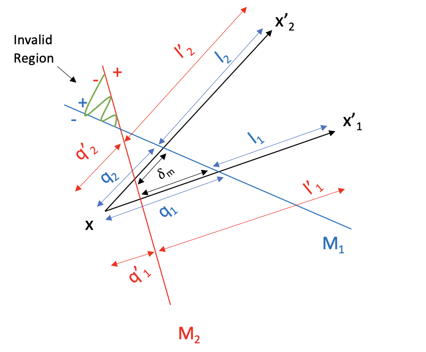
Figure 1: Abstract Diagramatic Representation of $\mathcal{M}_{1}$ and $\mathcal{M}_{2}$, with a data point $\mathcal{S}$ represented by feature-vector $x$ and two potential feature vectors $x^{\prime}_{1}$ and $x^{\prime}_{2}$ denoting possible recourse $\mathcal{S^{\prime}}$.

To show that there is a trade-off between cost and invalidation percentage, we need to determine that recourses with lower costs are at high risk of invalidation, and vice-versa. Our analysis considers sparse counterfactual style recourses, presuming cost to be represented by the common Euclidean notion of distance. Our notation is illustrated in figure 1 below, defining $x$ as the data point, and $x^{\prime}_{1}$ and $x^{\prime}_{2}$ as two potential recourses. We consider the model $\mathcal{M}_{2}$ to be defined as a perturbation of model $\mathcal{M}_{1}$ by some arbitrary magnitude $\delta_{m}$. Distances (measured according to the generic cost metric $d$) are measured along the vectors $x\rightarrow x^{\prime}_{1}$ and $x\rightarrow x^{\prime}_{2}$: $q_{1}$ and $q_{2}$ from $x$ to $\mathcal{M}_{1}$, and $l_{1}$ and $l_{2}$ from $\mathcal{M}_{1}$ to $x^{\prime}_{1}$ and $x^{\prime}_{2}$ respectively. We similarly have $q^{\prime}_{1}$ and $q^{\prime}_{2}$ from $x$ to $\mathcal{M}_{2}$, and $l^{\prime}_{1}$ and $l^{\prime}_{2}$ from $\mathcal{M}_{2}$ to $x^{\prime}_{1}$ and $x^{\prime}_{2}$ respectively. The cost function with L2 norm is very common in sparse counterfactuals, defined as $d(x,x^{\prime})=||x-x^{\prime}||_{2}$ (Wachter et al. (2018)). Lastly, we denote the probability of invalidation for an arbitrary recourse $x^{\prime}$ under model $\mathcal{M}_{2}$ as $Q_{x^{\prime}}=\frac{1-\mathcal{M}_{2}(x^{\prime})}{2}$. Note that by the definition of recourse, $\mathcal{M}_{1}(x^{\prime})=+1$ and $\mathcal{M}_{2}(x^{\prime})=+1$ for valid recourses but $\mathcal{M}_{2}(x^{\prime})=-1$ for invalid recourses.

Theorem 3.1.

If we have recourses $x^{\prime}_{1}$ and $x^{\prime}_{2}$ for a data point $x$ and model $\mathcal{M}_{1}$, such that $d(x,x^{\prime}_{1})\leq d(x,x^{\prime}_{1})$ then the respective expected probabilities of invalidation under model $\mathcal{M}_{2}$, $Q_{\mathbb{E}\left[x^{\prime}_{1}\right]}$ and $Q_{\mathbb{E}\left[x^{\prime}_{2}\right]}$, follow $Q_{\mathbb{E}\left[x^{\prime}_{1}\right]}\geq Q_{\mathbb{E}\left[x^{\prime}_{2}\right]}$.

Proof (Sketch).

We know from our construction that $d(x,x^{\prime}_{1})=q_{1}+l_{1}$ and $d(x,x^{\prime}_{2})=q_{2}+l_{2}$, and also that $l^{\prime}_{1}=l_{1}\pm\delta_{m}$ and $l^{\prime}_{2}=l_{2}\pm\delta_{m}$. We assume that the small random perturbation $\delta_{m}$ between $\mathcal{M}_{1}$ and $\mathcal{M}_{2}$ has expected value $\mathbb{E}[\delta_{m}]=0$. Further, we also assume that both $q_{1}$ and $q_{2}$ are random variables drawn from the same unknown distribution, with some arbitrary expected value $\bar{q}=\mathbb{E}\left[q_{1}\right]=\mathbb{E}\left[q_{2}\right]$.

Thus, referring to figure 1 we get: $d(x,x^{\prime}_{1})\leq d(x,x^{\prime}_{2})\implies\mathbb{E}\left[q_{1}+l_{1}\right]\leq\mathbb{E}\left[q_{2}+l_{2}\right]\implies\mathbb{E}\left[l_{1}\right]\pm\mathbb{E}\left[\delta_{m}\right]\leq\mathbb{E}\left[l_{2}\right]\pm\mathbb{E}\left[\delta_{m}\right]\implies\mathbb{E}\left[l^{\prime}_{1}\right]\leq\mathbb{E}\left[l^{\prime}_{2}\right]$

To capture the notion that models are less confident in their predictions on points close to their decision boundaries, we construct a function $g(l^{\prime})=P\left[\mathcal{M}_{2}(x^{\prime})=+1\right]$, using the bijective relationship between $x^{\prime}$ and $l^{\prime}$. Therefore, $g$ is a monotonically increasing function, with $g(l^{\prime})=-Q_{x^{\prime}}$.

We now equate the probability of invalidation $Q$ to an arbitrary function $g(l^{\prime})$. The bijection between $x^{\prime}$ and $l^{\prime}$ allows us to define $g(l^{\prime})=-Q(x^{\prime})$ as a monotonic increasing function, with $g(-\infty)=0$, $g(-\delta_{m})<=0.5$, $g(\delta_{m})>=0.5$, and $g(\infty)=1$. We can now apply this monotonic increasing function and continue our derivation to get: $g(\mathbb{E}\left[l^{\prime}_{1}\right])\leq g(\mathbb{E}\left[l^{\prime}_{2}\right])\implies Q_{\mathbb{E}\left[x^{\prime}_{1}\right]}\geq Q_{\mathbb{E}\left[x^{\prime}_{2}\right]}$. A detailed proof is included in the Appendix. ∎

Proposition 3.2.

There is a tradeoff between recourse costs (with respect to model $\mathcal{M}_{1}$) and recourse invalidation percentages (with respect to the updated model $\mathcal{M}_{2}$). Consider a hypothetical function $F$ that computes recourse costs $d(x,x^{\prime})$ from expected invalidation probabilities $Q_{\mathbb{E}\left[x^{\prime}\right]}$. Therefore $F\left[Q_{\mathbb{E}\left[x^{\prime}\right]}\right]=d(x,x^{\prime})$ is a monotonically decreasing function: as invalidation probabilities increase (or decrease), recourse costs decrease (or increase), and vice versa.

Proof (Sketch).

Consider a hypothetical function $G=F^{-1}$ such that $G\left[d(x,x^{\prime})\right]=Q_{\mathbb{E}\left[x^{\prime}\right]}$. From the proof of theorem 3.1 above we know that $d(x,x^{\prime}_{1})\leq d(x,x^{\prime}_{2})\implies Q_{\mathbb{E}\left[x^{\prime}_{1}\right]}\geq Q_{\mathbb{E}\left[x^{\prime}_{2}\right]}$. Thus $G$ is monotonic, and it’s hypothetical inverse $F$ must also be monotonic (if it exists). A detailed proof is included in the Appendix. ∎

For decision makers, this has key implications: cheaper costs $d(x,x^{\prime}_{1})$ imply higher invalidation chances $Q_{\mathbb{E}\left[x^{\prime}_{1}\right]}$, and more expensive costs $d(x,x^{\prime}_{2})$ imply lower invalidation chances $Q_{\mathbb{E}\left[x^{\prime}_{2}\right]}$. The contrapositives of these statements also hold, meaning that low invalidation probabilities imply more expensive recourse costs, and that high invalidation probabilities imply cheaper recourse costs. Therefore, we can say that there exists a tradeoff between recourse costs and invalidation probabilities.

This establishes that recourses that have lower costs are more likely to get invalidated by the updated model $\mathcal{M}_{2}$. This is a critical result that demonstrates a fundamental flaw in the design of state-of-the-art recourse finding algorithms since the objective formulations in these algorithms explicitly try to minimize these costs. By doing so, these algorithms are essentially generating recourses that are more likely to be invalidated upon model updation.

3.4 Lower Bounds on Recourse Invalidation Probabilities

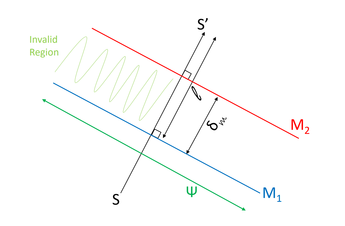
Figure 2: Parallel model perturbation of arbitrary magnitude $\delta_{m}$ between linear models $\mathcal{M}_{1}$ and $\mathcal{M}_{2}$. The range of the data is represented by manifold $\Psi$.

In order to find general lower bounds on the probability of invalidation for recourses $\mathcal{CF}_{1}$ under $\mathcal{M}_{2}$, we first cast the couunterfactual search procedure as a Markov Decision Process, and then use this observation to hypothesize about the distributions of the recourses $\mathcal{CF}_{1}$. We then use these distributions to derive the lower bounds on the invalidation probability.

Proposition 3.3.

The search process employed by state-of-the-art sparsity based recourse generation algorithms (e.g., Wachter et al. (2018)) is a Markov Decision Process.

Proof (Sketch).

We know that the search for counterfactual explanations consists of solving the optimization problem given by $\arg\min_{\mathcal{S^{\prime}}}{d(\mathcal{S^{\prime}},\mathcal{S})}$, where sparse counterfactuals are unrestricted, and data support counterfactuals are restricted to the set ${\mathcal{S^{\prime}}:P_{data}(\mathcal{S^{\prime}})>0}$. The search procedure moves through the path $\mathcal{S}\rightarrow\cdots\mathcal{S"}\cdots\rightarrow\mathcal{S^{\prime}}$, looping through different possible values of $\mathcal{S"}$ until $\mathcal{M}_{1}(\mathcal{S"})=+1$ and cost $d(\mathcal{S},\mathcal{S"})$ is minimized - at which point the recourse $\mathcal{S^{\prime}}=\mathcal{S"}$ is returned. For sparse counterfactuals, each step in this search depends only on the previous iteration, and not on the entire search path so far, that is: $P(\mathcal{S"}_{t+1}|\mathcal{S"}_{t},\mathcal{S"}_{t-1}\dots\mathcal{S})=\mathcal{S"}_{t+1}|\mathcal{S"}_{t}$. Thus, by satisfying this condition, the recourse generation technique is a Markov Decision Process. A detailed proof is included in the Appendix. ∎

Lemma 3.4.

If the model $\mathcal{M}_{1}$ is linear, then the distribution of recourses $\mathcal{CF}_{1}$ is exponential for continuous (numeric) data or geometric for categorical (ordinal) data, along the normal to the classifier hyperplane. Thus for $\mathcal{S^{\prime}}\in\mathcal{CF}_{1}$, we have $l\sim L$ with $f(l)=\rho\cdot e^{-\rho l}$ or $f(l)=(1-\rho)^{l-1}\cdot\rho$, where $L$ is the distance from $\mathcal{S^{\prime}}$ to $\mathcal{M}_{1}$ (figure 2).

Proof (Sketch).

By Proposition 3.3 above, we know that the recourse search process follows the Markov Property, and thus the distribution of the recourses must have the memoryless property. Further, since the classifier is linear, we know that an unrestricted recourse search, such as that of sparse counterfactual based recourses, will proceed exactly along the normal to the classifier hyperplane, in the direction of increasingly positive $\mathcal{M}_{1}$ classification probabilities. Lastly, we assume that the probability of the counterfactual explanation search ending at any given iteration $t$ with $\mathcal{S^{\prime}}=\mathcal{S"}_{t}$ is always constant $\rho$. Thus, for continuous data, the distribution of recourses is exponential with $\lambda=\rho$, and for ordinal data the distribution is geometric with parameter $p=\rho$. A detailed proof is included in the Appendix. ∎

Theorem 3.5.

For a given linear model $\mathcal{M}_{1}$ with recourses $\mathcal{CF}_{1}$, and a parallel linear model $\mathcal{M}_{2}$ with arbitrary (constant) perturbation $\delta_{m}$, the invalidation probabilities $Q{{}_{\mathcal{S^{\prime}}}}$ are $1-e^{-\rho\delta_{m}}$ for continuous (numeric) data, and $1-(1-\rho)^{\delta_{m}}$ for categoric (ordinal) data.

Proof (Sketch).

Let the recourses be distributed according to some unknown arbitrary distribution with density $f(l)$, where $l\in(0,\infty)$ is the normal distance between $\mathcal{M}_{1}$ and $\mathcal{S^{\prime}}$. Then, as is clear from the invalid region between the models $\mathcal{M}_{1}$ and $\mathcal{M}_{2}$ illustrated in figure 2, the probability of invalidation of the recourses $\mathcal{S^{\prime}}$ is $Q_{\mathcal{S^{\prime}}}=\frac{1}{\Psi}\int_{\Psi}\left[\int_{0}^{\delta_{m}}f(l)\,dl\right]\,d\psi$. Here $\psi$ is an arbitrary element of the decision boundary, within the data manifold $\Psi$.

We can now combine this result with known distributions from Lemma 3.4 to get: $Q_{\mathcal{S^{\prime}}}=\frac{1}{\Psi}\int_{\Psi}\left[\int_{0}^{\delta_{m}}\rho e^{-\rho l}\,dl\right]\,d\psi=1-e^{-\rho\delta_{m}}$ for continuous features, and $Q_{\mathcal{S^{\prime}}}=\frac{1}{\Psi}\int_{\Psi}\left[\sum_{l=1}^{\delta_{m}}(1-\rho)^{l-1}\cdot\rho\right]\,d\psi=1-(1-\rho)^{\delta_{m}}$ for ordinal features. A detailed proof is included in the Appendix. ∎

Theorem 3.6.

For a given nonlinear model $\mathcal{M}_{1}$ with recourses $\mathcal{CF}_{1}$, and a parallel nonlinear model $\mathcal{M}_{2}$ with known constant perturbation $\delta_{m}$, the lower bound on the invalidation probabilities is achieved exactly when both models $\mathcal{M}_{1}$ and $\mathcal{M}_{2}$ are linear.

Proof (Sketch).

We consider a piecewise linear approximation of the nonlinear models, with an arbitrary degree of precision. At each point in the classifier decsion boundary, we consider the piecewise linear approximation to make an angle $\theta$ with a hypothetical hyperplane in the data manifold $\Psi$. We then proceed identically as in the proof for theorem 3.5 above, with $Q_{\mathcal{S^{\prime}}}=\frac{1}{\Psi\cos\theta}\int_{\Psi}\left[\int_{0}^{\delta_{m}}f(l)\,dl\right]\,d\psi$, where the extra $\cos\theta$ term reflects that the models are locally inclined at an angle $\theta$ from the hyperplane $\psi$.

It is easy to see that $Q_{\mathcal{S^{\prime}}}$ will be maximized when $\theta=0,\forall\theta$, because $\frac{dQ_{\mathcal{S^{\prime}}}}{d\theta}\propto\tan\theta=0\implies\theta=0$. If each element of the piecewise linear approximation makes a constant angle of $0$ with the models, then the models themselves must be linear. Thus, the lower bound on invalidation probability for non-linear models must exactly be the invalidation probability for linear models, given the same data (manifold). A detailed proof is included in the Appendix. ∎

Combining the last two results, for any arbitrary model $\mathcal{M}_{1}$, we know that another model $\mathcal{M}_{2}$ perturbed parallelly with magnitude would cause invalidation with the following lower bounds: $Q_{\mathcal{S^{\prime}}}\geq 1-e^{-\rho\delta_{m}}$, for continuous data and $Q_{\mathcal{S^{\prime}}}\geq 1-(1-\rho)^{\delta_{m}}$ for ordinal data.

4 Experimental Analysis

In this section we analyze recourse invalidation caused by model updates made due to naturally occurring real world distribution shifts. In our experiments we consider recourse generation methods that either directly optimise cost (sparse counterfactuals, such as Wachter et al. (2018)), promote recourses that lie in-distribution (data support counterfactuals, such as Ustun et al. (2019)), or are generated from an assumed underlying structural causal model of the data (causal counterfactuals, such as Karimi et al. (2020b)). We also use synthetically generated datasets to perform a sensitivity analysis to further understand how the magnitude of distribution shifts affects the proportion of recourses being invalidated.

Setup

: We consider an initial dataset $\mathcal{D}_{1}$ upon which we train model $\mathcal{M}_{1}$, and a dataset $\mathcal{D}_{2}$ in which the distribution has shifted, upon which we train model $\mathcal{M}_{2}$. We reserve 10% of both datasets for validation in order to perform sanity checks on the accuracies of our models $\mathcal{M}_{1}$ and $\mathcal{M}_{2}$. We then follow the experimental setup described in 3.2 for various model types: Logistic Regression (LR), Random Forests (RF), Gradient Boosted Trees (XGB), Linear Support Vector Machines (SVM), a small Neural Network with hidden layers = [10, 10, 5] (DNN (s)), and a larger Neural Network with hidden layers = [20, 10, 10, 10, 5] (DNN (l)). The models are all treated as binary classification black-boxes with adversely classified ($\{\mathcal{S}\in\mathcal{D}_{1}:\mathcal{M}_{1}(\mathcal{S})=-1\}$) people being provided recourses $\mathcal{S^{\prime}}\in\mathcal{CF}_{1}$. Finally, we check how many of the recourses from $\mathcal{CF}_{1}$ are still classified adversely by the updated prediction model $\mathcal{M}2$, that is $\{\mathcal{S^{\prime}}\in\mathcal{CF}_{1}:\mathcal{M}_{2}(\mathcal{S^{\prime}})=-1\}$. We hope that 0% of $\mathcal{CF}_{1}$ has been invalidated, allowing the decision maker to keep their promise to the users when recourse was initially provided.

We conduct this entire experiment with two different recourse generation techniques: counterfactual explanations (hencefore CFE), from Wachter et al. (2018); and actionable recourse (henceforth AR), from Ustun et al. (2019), details of which are included in section 2. To adapt CFE to non-differentiable models we use numeric differentiation and approximate gradients, and to adapt AR to non-linear models we use a local linear model approximation using LIME (Ribeiro et al. (2016)). These are standard baseline adaptations we adapt from prior works. When structural causal models are known (although this is often difficult in real world applications), we also perform experiments using Karimi et al. (2020b). Our results containing 10-fold cross-validation accuracies for models $\mathcal{M}_{1}$ and $\mathcal{M}_{2}$ and the respective invalidation proportions are summarized in table 1 below. We will be releasing the code used to produce these results, including hyperparameter settings, infrastructure requirements, and runtimes, as open-source via GitHub.

Datasets

: We conduct our analysis using three different real world datasets, each from a different "high-stakes" domain, to show the real world impact of our findings. The first dataset is from the domain of criminal justice (Lakkaraju et al. (2016)), which contains proprietary data from 1978 ($\mathcal{D}_{1}$ - 8395 points) and 1980 ($\mathcal{D}_{2}$ - 8595 points) respectively. This dataset contains demographic features such as race, sex, age, time-served, and employment, and a target attribute corresponding to bail decisions. This data contains an inherent Temporal dataset shift, as the character of the data in 1980 differs from the data in 1978. Our second dataset is from the education domain, and consists of publically available student data collected from schools in Jordan ($\mathcal{D}_{1}$ - 129 points) and Kuwait ($\mathcal{D}_{2}$ - 122). We consider the problem of predicting grades (binary classification between pass and fail) using input predictors such as grade, holidays-taken, and class-participation (Aljarah (2016)). This data contains an inherent Geospatial distribution shift as the character of student data varies across countries. Lastly, from the domain of finance, we consider the publically available German credit dataset ($\mathcal{D}_{1}$ - 900 points) (Dua and Graff (2017)), along with its updated version ($\mathcal{D}_{2}$ - 900 points) (Grömping (2019)). This This is a credit scoring problem using features such as the applicants loan amount, employment history, and age as predictors. The data here represents a Data Correction based distribution shift, as the character of the data can be said to change due to a change in the data preprocessing step. Unlike the previous datasets, in this case we also have access to an underlying causal model from Karimi et al. (2020b), and we are thus able to additionally perform experiments using the causal recourse generation algorithm proposed here.

		Temporal Shift			Geospatial Shift			Data Correction Shift
Algorithm	Model	M1 acc	M2 acc	Inv. %	M1 acc	M2 acc	Inv. %	M1 acc	M2 acc	Inv. %
AR	LR	94	95.4	96.6	88	93	76.6	71	75	7.79
	RF	99	99.5	0.05	89	92	NAN	73	73	35
	XGB	100	99.7	0	85	93	NAN	74	75	8
	SVM	81	78.9	3.05	80	91	90	63	69	100
	DNN (s)	99	99.4	19.26	83	87	NAN	68	69	NAN
	DNN (l)	99	99.6	0	82	93	NAN	66	67	0
CFE	LR	94	95.4	98.29	88	93	65.96	71	75	3.9
	RF	99	99.5	0.71	89	92	76.47	73	73	36.82
	XGB	100	99.7	0.46	85	93	57.14	74	75	23.72
	SVM	81	78.9	100	80	91	100	63	69	0
	DNN (s)	99	99.4	91.38	83	87	50	68	69	NAN
	DNN (l)	99	99.6	0.13	82	93	30.3	66	67	0
Causal	LR							69	71	0
	RF		unknown			unknown		65	64	96.09
	XGB		causal			causal		64	68	12.5
	DNN (s)		model			model		69	70	NAN
	DNN (l)							69	70	NAN

Table 1: Recourse Invalidation Proportions caused by Model Updates due to various (Temporal, Geospatioal, or Data Correction) Distribution Shifts.

Temporal Distribution Shifts

: Columns 3, 4, and 5 showcase the results on the bail dataset from the criminal justice domain, which contains a temporal distribution shift. We can see that most models have high (> 95%) accuracy, and yet the invalidation proportions vary significantly between AR and CFE, however this trend does not seem to be corellated with model accuracies. While there are some cases with no invalidation, the CFE algorithm, when applied to an SVM model, creates a situation where all of the recourses generated end up getting invalidated. This clearly demonstrates the potential harm of recourse invalidation. We are unable to perform experiments using a causal recourse generation technique because the underlying causal distribution is unknown for this dataset.

Geospatial Distribution Shifts

: Columns 6, 7, and 8 showcase results on the schools dataset from the education domain, which contains a geospatial data distribution shift. We see a minimum invalidation of 30% on this dataset, indicating there are no good situations for a decision maker to provide algorithmic recourses in the scenario. We see multiple NAN values for recourse invalidation for the AR method on this dataset. These represent those situations when no recourses could be generated (that is, $\mathcal{CF}_{1}$ is empty, and thus the proportion of recourses from $\mathcal{CF}_{1}$ that are invalidated is undefined). We also see here that even though model accuracies are increasing, recourse invalidation remains an observable issue, indicating that this phenomenon cannot be explained away as a modelling error made by decision makers, but instead is inherent to distribution shifts. The lack of an underlying structural causal model again precludes us from being able to conduct experiments using causal recourse generation techniques on this data.

Data Correction Distribution Shifts

: Columns 9, 10, and 11 showcase results on the German credit datasets, which contain a data-correction related distribution shifts. Often decision makers might initially deploy a model trained on inaccurate or corrupt data, or data that suffers from selection biases. As the decision makers improve their training datasets and redeploy their models, a distribution shift would occur, which is captured by this experiment. Again, NAN values indicate that no recourses were found, and thus the proportion of those invalidated is undefined. Here, we see extreme behaviour - SVM shows 100% invalidation with AR, but 0% with CFE. On the other hand, XGB has higher invalidation with CFE than with AR. This further demonstrates that the phenomenon of recourse invalidation is independent of model types or specific recourse generation algorithms. Lastly, we see that even causally generated recourses are vulnerable to the problem of recourse invalidation. Interestingly, the RF and XGB models are the worst affected, even though the temporal distribution shift results might have led us to believe these were the most robust models. Thus, it appears that the advantages (Karimi et al. (2020a); Venkatasubramanian and Alfano (2020); Barocas et al. (2020)) of causally generated recourses over other recourse generation algorithms do not protect us from recourse invalidation due to model updates caused by distribution shifts.

Sensitivity Analysis

: We have demonstrated empirically that distribution shifts cause recourse invalidation, and we now wish to qualify whether larger distribution shifts lead to greater recourse invalidation. To do this we construct synthetic datasets and precisely control the type of distribution shift. We start with a fixed distribution $\mathcal{D}_{1}$, which has two independent predictors $X0$ and $X1$, both drawn from a standard normal distribution, with the binary target attribute defined linearly as $Y=(X0+X1\geq 0)$. We then train a logistic regression model $\mathcal{M}_{1}$ and generate recourses $\mathcal{CF}_{1}$ from either AR or CFE. Finally, we shift the distribution $\mathcal{D}_{2}$ according to some shift parameter $\alpha$ and construct logistic regression model $\mathcal{M}_{2}$, and analyse the relation between recourse invalidation percentage and $\alpha$. We consider two scenarios, with a shift parameter $\alpha$ defining amount of shift between $\mathcal{D}_{2}$ and $\mathcal{D}_{1}$:

1. Shifting target: where the predictor distribution ($X0$ and $X1$) stays constant, but the $\mathcal{D}_{2}$ target attribute is defined as $Y=(X0+\alpha X1\geq 0)$, for a % shift of $\alpha\in(-60\%,60\%)$.

2. Shifting predictors: where the definition of the target stays constant ($Y=(X0+X1\geq 0)$), but we shift the mean of the predictor distribution in $\mathcal{D}_{2}$ from $(X0,X1)=(0,0)$ to $(X0,X1)=(\alpha,\alpha)$.

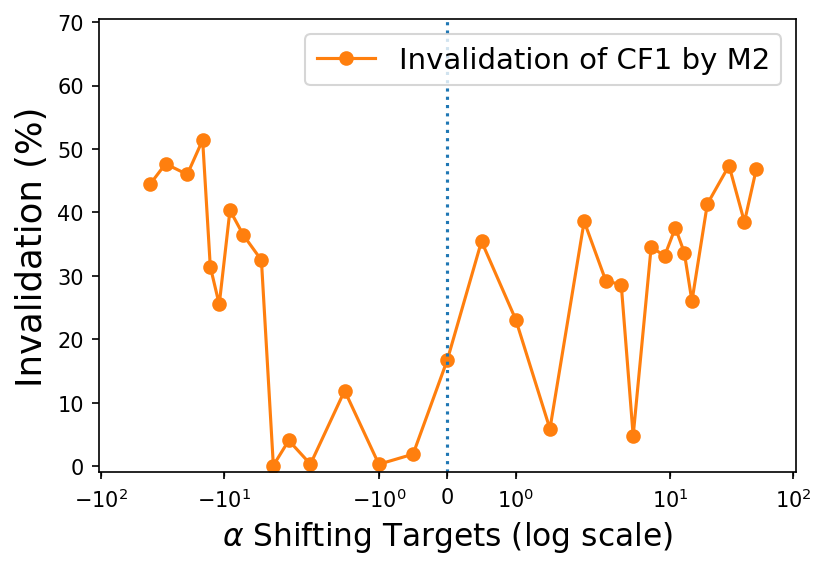
(a) Recourse Invalidation vs Drifting Targets [AR]

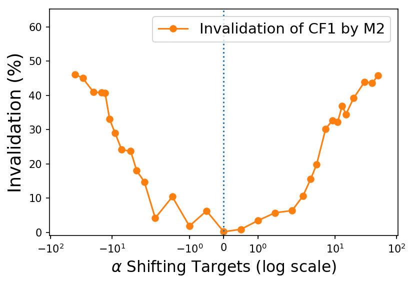
(b) Recourse Invalidation vs Drifting Targets [CFE]

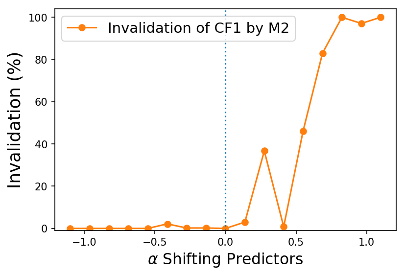
(c) Recourse Invalidation vs Drifting Predictors [AR]

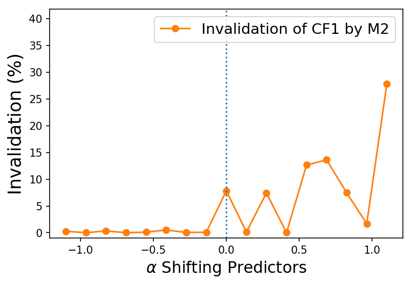
(d) Recourse Invalidation vs Drifting Predictors [CFE]

Figure 3: Sensitivity Analysis: Recourse Invalidation Increases with Increasing Drift. (All models have accuracy > 99%)

As figures 3(a) through 3(d) demonstrate, recourse invalidation increases with increasing distribution shift, but this is not universal. There may be some distribution shifts that the recourses generated are robust to, and others that result in upto 100% of generated recourses getting invalidated. Particularly, when $\alpha$ is negative while shifting predictors (with this particular target distribution), recourses generated are robust. In all other cases there is significant invalidation that increases with increasing $\alpha$. It is also noteworthy that even with data support based counterfactual recourse AR, we do not uniformly see less invalidation, as postulated by Ustun et al. (2019). Sometimes the recourses generated are indeed more robust, but they also often fail miserably with up to 100% invalidation. This would suggest that data support counterfactual based recourses are actually less predictable than sparse counterfactual based recourses, while still being vulnerable to invalidation, and could thus potentially be more risky for real world decision makers.

5 Conclusion

In this paper, we analyse the impact of distribution shifts on recourses generated by state-of-the-art algorithms. We conduct multiple real world experiments and show that distribution shifts can cause significant invalidation of generated recourses, jeopardizing trust in decision makers. This is contrary to the goals of a decision maker providing recourse to their users. We show theoretically that there is a trade-off between minimising cost and providing robust, hard-to-invalidate recourses when using sparse counterfactual generation techniques. We also find the lower bounds on the probability of invalidation of recourses when model updates are of known perturbation magnitude. While our theory pertains only to sparse counterfactual based recourses, we demonstrate experimentally that invalidation problems due to distribution shift persist in practice not only with data support based counterfactual recourse, but also with causally generated recourses. Theoretical examination of recourse invalidation when using these recourse generation methods remains as future work.

This work paves the way for several other interesting future directions too. It would be interesting to develop novel recourse finding strategies that do not suffer from the drawbacks of existing techniques and are robust to distribution shifts. This could involve iteratively finding and examining recourses as part of the model training phase, in order to ensure that recourses with high likelihood of invalidation are never prescribed after model deployment.

Appendix A Theoretical Analysis

A.1 Preliminaries

We consider a black box binary classifier $\mathcal{M}$ trained on a dataset of real world users $\mathcal{D}$ and for each user $\mathcal{S}$ in $\mathcal{D}$, let us consider the corresponding recourse found by a recourse generation algorithm $Alg$ to be $\mathcal{S^{\prime}}$.

Further, let the set of adversely (negatively) classified users be $\mathcal{D}^{M-}$, positively classified users be $\mathcal{D}^{M+}$, and the set of all recourses be $\mathcal{CF}_{1}$. Our definitions can be thus written as follows:

$$\mathcal{D}^{M+} =\{\mathcal{S}\in\mathcal{D}:\mathcal{M}(\mathcal{S})=+1\}$$ (6)

$$\mathcal{D}^{M-} =\{\mathcal{S}\in\mathcal{D}:\mathcal{M}(\mathcal{S})=-1\}$$ (7)

$$\mathcal{CF}_{1} =\{\mathcal{S}\in\mathcal{D}^{M-},\mathcal{S^{\prime}}:Alg(\mathcal{S})=\mathcal{S^{\prime}}\}$$ (8)

From our construction the following three statements always hold:

$$\mathcal{M}(\mathcal{S}) =-1\;\;\forall\;\;\mathcal{S}\in\mathcal{D}^{M-}$$ (9)

$$\mathcal{M}(\mathcal{S}) =+1\;\;\forall\;\;\mathcal{S}\in\mathcal{D}^{M+}$$ (10)

$$\mathcal{M}(\mathcal{S^{\prime}}) =+1\;\;\forall\;\;\mathcal{S^{\prime}}\in\mathcal{CF}_{1}$$ (11)

All recourse generation methods essentially perform a search starting from a given data point $\mathcal{S}$, going towards $\mathcal{S^{\prime}}$, by repeatedly polling the input-space of the black box model $\mathcal{M}$ along the path $\mathcal{S}\rightarrow\cdots\mathcal{S"}\cdots\rightarrow\mathcal{S^{\prime}}$. There are many ways in which to guide this path when searching for counterfactual explanations. Sparse recourse generation techniques (Pawelczyk et al. [2020a]) operate on a given data point $\mathcal{S}$, and an arbitrary cost function $d(\mathcal{S},\mathcal{S^{\prime}})$ (usually set to $d(\mathcal{S},\mathcal{S^{\prime}})=||\mathcal{S}-\mathcal{S^{\prime}}||_{p}$, $p\in\{1,2\}$). For example, Wachter et al. [2018] define optimal recourses according to eqn 12. Data support recourses restrict the counterfactual search to those $\mathcal{S^{\prime}}$ that are found in the data distribution (with high probability), as in eqn 13. Ustun et al. [2019] use a heuristic to try and optimise this using linear programming tools.

$$\mathcal{S^{\prime}} =\arg\min_{\mathcal{S^{\prime}}}\,{d(\mathcal{S},\mathcal{S^{\prime}})}$$ (12)

$$\mathcal{S^{\prime}} =\arg\min_{\mathcal{S^{\prime}}:P_{data}(\mathcal{S^{\prime}})>0}\,{d(\mathcal{S},\mathcal{S^{\prime}})}$$ (13)

A.2 The Cost vs Invalidation Trade-off

To show that there is a trade-off between cost and invalidation percentage, we need to determine that recourses with lower costs are at high risk of invalidation, and vice-versa. Our analysis considers sparse counterfactual style recourses Pawelczyk et al. [2020a], presuming cost to be represented by the common Euclidean notion of distance. Our notation is illustrated in figure 4 below, defining $x$ as the data point, and $x^{\prime}_{1}$ and $x^{\prime}_{2}$ as two potential recourses. We consider the model $\mathcal{M}_{2}$ to be defined as a perturbation of model $\mathcal{M}_{1}$ by some arbitrary magnitude $\delta_{m}$. Distances (measured according to the generic cost metric $d$) are measured along the vectors $x\rightarrow x^{\prime}_{1}$ and $x\rightarrow x^{\prime}_{2}$: $q_{1}$ and $q_{2}$ from $x$ to $\mathcal{M}_{1}$, and $l_{1}$ and $l_{2}$ from $\mathcal{M}_{1}$ to $x^{\prime}_{1}$ and $x^{\prime}_{2}$ respectively. We similarly have $q^{\prime}_{1}$ and $q^{\prime}_{2}$ from $x$ to $\mathcal{M}_{2}$, and $l^{\prime}_{1}$ and $l^{\prime}_{2}$ from $\mathcal{M}_{2}$ to $x^{\prime}_{1}$ and $x^{\prime}_{2}$ respectively. The cost function with L2 norm is very common in sparse counterfactuals, defined as $d(x,x^{\prime})=||x-x^{\prime}||_{2}$Wachter et al. [2018]. Lastly, we denote the probability of invalidation for an arbitrary recourse $x^{\prime}$ under model $\mathcal{M}_{2}$ as $Q_{x^{\prime}}=\frac{1-\mathcal{M}_{2}(x^{\prime})}{2}$. Note that by the definition of recourse, $\mathcal{M}_{1}(x^{\prime})=+1$ and $\mathcal{M}_{2}(x^{\prime})=+1$ for valid recourses but $\mathcal{M}_{2}(x^{\prime})=-1$ for invalid recourses.

Figure 4: Abstract Diagramatic Representation of $\mathcal{M}_{1}$ and $\mathcal{M}_{2}$, with a data point $\mathcal{S}$ represented by feature-vector $x$ and two potential feature vectors $x^{\prime}_{1}$ and $x^{\prime}_{2}$ denoting possible recourse $\mathcal{S^{\prime}}$.

Theorem A.1.

If we have recourses $x^{\prime}_{1}$ and $x^{\prime}_{2}$ for a data point $x$ and model $\mathcal{M}_{1}$, such that $d(x,x^{\prime}_{1})\leq d(x,x^{\prime}_{1})$ then the respective expected probabilities of invalidation under model $\mathcal{M}_{2}$, $Q_{\mathbb{E}\left[x^{\prime}_{1}\right]}$ and $Q_{\mathbb{E}\left[x^{\prime}_{2}\right]}$, follow $Q_{\mathbb{E}\left[x^{\prime}_{1}\right]}\geq Q_{\mathbb{E}\left[x^{\prime}_{2}\right]}$.

Proof.

We know from our construction that $d(x,x^{\prime}_{1})=q_{1}+l_{1}$ and $d(x,x^{\prime}_{2})=q_{2}+l_{2}$, and also that $l^{\prime}_{1}=l_{1}\pm\delta_{m}$ and $l^{\prime}_{2}=l_{2}\pm\delta_{m}$. We assume that the small random perturbation $\delta_{m}$ between $\mathcal{M}_{1}$ and $\mathcal{M}_{2}$ has expected value $\mathbb{E}[\delta_{m}]=0$. Further, we also assume that both $q_{1}$ and $q_{2}$ are random variables drawn from the same unknown distribution, with some arbitrary expected value $\bar{q}=\mathbb{E}\left[q_{1}\right]=\mathbb{E}\left[q_{2}\right]$.

$$d(x,x^{\prime}_{1}) \leq d(x,x^{\prime}_{2})$$ (14)

$$q_{1}+l_{1} \leq q_{2}+l_{2}$$ (15)

$$\mathbb{E}\left[q_{1}+l_{1}\right] \leq\mathbb{E}\left[q_{2}+l_{2}\right]$$ (16)

$$\mathbb{E}\left[q_{1}\right]+\mathbb{E}\left[l_{1}\right] \leq\mathbb{E}\left[q_{2}\right]+\mathbb{E}\left[l_{2}\right]$$ (17)

$$\bar{q}+\mathbb{E}\left[l_{1}\right] \leq\bar{q}+\mathbb{E}\left[l_{2}\right]$$ (18)

$$\mathbb{E}\left[l_{1}\right] \leq\mathbb{E}\left[l_{2}\right]$$ (19)

$$\mathbb{E}\left[l_{1}\right]\pm 0 \leq\mathbb{E}\left[l_{2}\right]\pm 0$$ (20)

$$\mathbb{E}\left[l_{1}\right]\pm\mathbb{E}\left[\delta_{m}\right] \leq\mathbb{E}\left[l_{2}\right]\pm\mathbb{E}\left[\delta_{m}\right]$$ (21)

$$\mathbb{E}\left[l_{1}\pm\delta_{m}\right] \leq\mathbb{E}\left[l_{2}\pm\delta_{m}\right]$$ (22)

$$\mathbb{E}\left[l^{\prime}_{1}\right] \leq\mathbb{E}\left[l^{\prime}_{2}\right]$$ (23)

To capture the notion that models are less confident in their predictions on points close to their decision boundaries, we construct a function $g(l^{\prime})=P\left[\mathcal{M}_{2}(x^{\prime})=+1\right]$, using the bijective relationship between $x^{\prime}$ and $l^{\prime}$. Therefore, $g$ is a monotonically increasing function, with $g(l^{\prime})=-Q_{x^{\prime}}$.

We now equate the probability of invalidation $Q$ to an arbitrary function $g(l^{\prime})$. The bijection between $x^{\prime}$ and $l^{\prime}$ allows us to define $g(l^{\prime})=-Q(x^{\prime})$ as a monotonic increasing function, with $g(-\infty)=0$, $g(-\delta_{m})<=0.5$, $g(\delta_{m})>=0.5$, and $g(\infty)=1$. Lastly, we can now apply this monotonic increasing function and continue our derivation as follows:

$$g(\mathbb{E}\left[l^{\prime}_{1}\right]) \leq g(\mathbb{E}\left[l^{\prime}_{2}\right])$$

$$-Q_{\mathbb{E}\left[x^{\prime}_{1}\right]} \leq-Q_{\mathbb{E}\left[x^{\prime}_{2}\right]}$$

$$Q_{\mathbb{E}\left[x^{\prime}_{1}\right]} \geq Q_{\mathbb{E}\left[x^{\prime}_{2}\right]}$$

which gives us the intended result. ∎

Proposition A.2.

There is a tradeoff between recourse costs (with respect to model $\mathcal{M}_{1}$) and recourse invalidation percentages (with respect to the updated model $\mathcal{M}_{2}$). Consider a hypothetical function $F$ that computes recourse costs $d(x,x^{\prime})$ from expected invalidation probabilities $Q_{\mathbb{E}\left[x^{\prime}\right]}$. Therefore $F\left[Q_{\mathbb{E}\left[x^{\prime}\right]}\right]=d(x,x^{\prime})$ is a monotonically decreasing function: as invalidation probabilities increase (or decreases), recourse costs decrease (or increase) and vice versa.

Proof.

Consider a hypothetical function $G=F^{-1}$ such that $G\left[d(x,x^{\prime})\right]=Q_{\mathbb{E}\left[x^{\prime}\right]}$. From the proof of theorem A.1 above we know that $d(x,x^{\prime}_{1})\leq d(x,x^{\prime}_{2})\implies Q_{\mathbb{E}\left[x^{\prime}_{1}\right]}\geq Q_{\mathbb{E}\left[x^{\prime}_{2}\right]}$. Thus $G$ is monotonic, and it’s hypothetical inverse $F$ must also be monotonic (if it exists). This implies: (1) cheaper costs $d(x,x^{\prime}_{1})$ imply higher invalidation chances $Q_{\mathbb{E}\left[x^{\prime}_{1}\right]}$, and also (2) that more expensive costs $d(x,x^{\prime}_{2})$ imply lower invalidation chances $Q_{\mathbb{E}\left[x^{\prime}_{2}\right]}$. We can also take contrapositives of these first two statements, giving us the third and fourth statement:

1. cheaper costs $\implies$ higher invalidation

2. more expensive costs $\implies$ lower invalidation

3. lower invalidation $\implies$ more expensive costs

4. higher invalidation $\implies$ cheaper costs

Taken together, these statements complete our proof and show that an increase (or decrease) in recourse invalidation probabilities must necessarily be accompanied by a decrease (or increase) in recourse costs respectively, and vice versa. Therefore, we can say that there exists a tradeoff between recourse costs and invalidation probabilities. ∎

A.3 Lower Bounds on Recourse Invalidation Probabilities

In order to find general lower bounds on the probability of invalidation for recourses $\mathcal{CF}_{1}$ under $\mathcal{M}_{2}$, we first cast the counterfactual search procedure as a Markov Decision Process, and then use this observation to hypothesize about the distributions of the recourses $\mathcal{CF}_{1}$. We then use these distributions to derive the lower bounds on the invalidation probability.

Proposition A.3.

The search process employed by state-of-the-art sparsity based recourse generation algorithms (e.g., Wachter et al. [2018]) satisfies the Markovian property and is a Markov Decision Process.

Proof.

We know that the search for counterfactual explanations consists of solving the optimization problem given by:

$$\arg\min_{\mathcal{S^{\prime}}}{d(\mathcal{S^{\prime}},\mathcal{S})}$$ (24)

where sparse counterfactuals are unrestricted, and data support counterfactuals are restricted to the set $\{\mathcal{S^{\prime}}:P_{data}(\mathcal{S^{\prime}})>0\}$.

The search procedure moves through the path $\mathcal{S}\rightarrow\cdots\mathcal{S"}\cdots\rightarrow\mathcal{S^{\prime}}$, looping through different possible values of $\mathcal{S"}$ until it reaches some $\mathcal{S^{\prime}}$ where $\mathcal{M}_{1}(\mathcal{S^{\prime}})=+1$ and cost $d(\mathcal{S},\mathcal{S^{\prime}})$ is minimized and then that recourse $\mathcal{S^{\prime}}$ is returned.

In case of methods generating sparse counterfactuals, each step in the search depends only on the previous iteration, and not on the entire search path so far, that is: $P(\mathcal{S"}_{t+1}|\mathcal{S"}_{t},\mathcal{S"}_{t-1}\dots\mathcal{S})=P(\mathcal{S"}_{t+1}|\mathcal{S"}_{t})$. Therefore, the search process employed by state-of-the-art sparsity based recourse generation algorithms satisfies the Markovian property.

Furthermore, the search process can also be modeled as a Markov Decision Process (MDP) represented by the 4-tuple $(S,A,P,R)$. Each possible counterfactual corresponds a state in the state space $S$ with the initial state being the original instance for which counterfactual must be found. The terminal states correspond to all those counterfactuals for which the model prediction turns out to be positive i.e., $\mathcal{M}_{1}(\mathcal{S^{\prime}})=+1$. The action set $A$ constitutes the changes that need to be made to go from one possible counterfactual to another (e.g., "age + 2 years"). Each action from any given state unambiguously and deterministically leads to a single new state. So, the transition probabilities in $P$ are either $0$ or $1$. Lastly, the reward function $R$ is defined as follows: If an action $a\in A$ from some state $s\in S$ leads to a terminal state (i.e., to a counterfactual for which model prediction is positive), then the immediate reward is $1$, otherwise the immediate reward is $0$.

Thus, the search process for sparsity based recourse generation techniques can be modeled as a Markov Decision Process. ∎

Lemma A.4.

If the model $\mathcal{M}_{1}$ is linear, then the distribution of the distances between the counterfactuals/recourses $\mathcal{CF}_{1}$ and the hyperplane of the classifier $\mathcal{M}_{1}$ follows the exponential distribution for continuous data and geometric distribution for discrete data i.e., $f(l)=\rho\cdot e^{-\rho l}$ or $f(l)=(1-\rho)^{l-1}\cdot\rho$, where $l$ is the distance from $\mathcal{S^{\prime}}$ to $\mathcal{M}_{1}$ (figure 5).

Proof.

By Proposition A.3 above, we know that the recourse search process follows the Markovian Property, and is therefore memoryless. Since this process is memoryless, it follows either exponential (continuous data) or geometric (discrete data) distributions since these are the only two memoryless distributions.

Further, since the classifier is linear, we know that an unrestricted recourse search, such as that of sparse counterfactual based recourses, will proceed exactly along the normal to the classifier hyperplane (Ustun et al. [2019]), in the direction of increasingly positive $\mathcal{M}_{1}$ classification probabilities.

Using the aforementioned insights and denoting the probability of the counterfactual explanation search ending at any given iteration $t$ with $\mathcal{S^{\prime}}=\mathcal{S"}_{t}$ is always constant $\rho$, we can write the distribution of the distances between the counterfactuals/recourses and the hyperplane of the classifier as:

$$f(l)\sim\rho\cdot e^{-\rho l}\text{ if the data is continuous }$$ (25)

$$f(l)=(1-\rho)^{l-1}\cdot\rho\text{ if the data is discrete }$$ (26)

∎

Figure 5: Parallel model perturbation of arbitrary magnitude $\delta_{m}$ between linear models $\mathcal{M}_{1}$ and $\mathcal{M}_{2}$. The range of the data is represented by manifold $\Psi$.

Theorem A.5.

For a given linear model $\mathcal{M}_{1}$ with recourses $\mathcal{CF}_{1}$, and a parallel linear model $\mathcal{M}_{2}$ with arbitrary (constant) perturbation $\delta_{m}$, the invalidation probabilities $Q{{}_{\mathcal{S^{\prime}}}}$ are $1-e^{-\rho\delta_{m}}$ for continuous (numeric) data, and $1-(1-\rho)^{\delta_{m}}$ for categorical (ordinal) data.

Proof.

Let the recourses be distributed according to some unknown arbitrary distribution with density $f(l)$, where $l\in(0,\infty)$ is the normal distance between $\mathcal{M}_{1}$ and $\mathcal{S^{\prime}}$. Then, as is clear from the invalid region between the models $\mathcal{M}_{1}$ and $\mathcal{M}_{2}$ illustrated in figure 5, the probability of invalidation of the recourses $\mathcal{S^{\prime}}$ is $Q_{\mathcal{S^{\prime}}}=\frac{1}{\Psi}\int_{\Psi}\left[\int_{0}^{\delta_{m}}f(l)\,dl\right]\,d\psi$. Here $\psi$ is an arbitrary element of the decision boundary, within the data manifold $\Psi$.

We can now combine this result with known distributions from Lemma A.4 to get:

$$Q_{\mathcal{S^{\prime}}} =\frac{1}{\Psi}\int_{\Psi}\left[\int_{0}^{\delta_{m}}f(l)\,dl\right]\,d\psi$$ (27)

$$=\frac{1}{\Psi}\int_{\Psi}\left[\int_{0}^{\delta_{m}}\rho e^{-\rho l}\,dl\right]\,d\psi$$ (28)

$$=\frac{1}{\Psi}\int_{\Psi}\left[1-e^{-\rho\delta_{m}}\right]\,d\psi$$ (29)

$$=\frac{1}{\Psi}\int_{\Psi}\,d\psi\cdot\left[1-e^{-\rho\delta_{m}}\right]$$ (30)

$$=1-e^{-\rho\delta_{m}}$$ (31)

Similarly, for ordinal data this would be $Q_{\mathcal{S^{\prime}}}=\frac{1}{\Psi}\int_{\Psi}\left[\sum_{l=1}^{\delta_{m}}(1-\rho)^{l-1}\cdot\rho\right]\,d\psi=1-(1-\rho)^{\delta_{m}}$. Thus, we have characterised the exact invalidation probabilities for parallel linear models $\mathcal{M}_{1}$ and $\mathcal{M}_{2}$, with known distance $\delta_{m}$. ∎

We now tend to the case of classifiers with non-linear decision boundaries.

Theorem A.6.

For a given nonlinear model $\mathcal{M}_{1}$ with recourses $\mathcal{CF}_{1}$, and a parallel nonlinear model $\mathcal{M}_{2}$ with known constant perturbation $\delta_{m}$, the lower bound on the invalidation probabilities is achieved exactly when both models $\mathcal{M}_{1}$ and $\mathcal{M}_{2}$ are linear.

Proof.

We consider a piecewise linear approximation of the nonlinear models, with an arbitrary degree of precision. At each point in the classifier decsion boundary, we consider the piecewise linear approximation to make an angle $\theta$ with a hypothetical hyperplane in the data manifold $\Psi$. We then proceed identically as in the proof for theorem A.5 above with:

$$Q_{\mathcal{S^{\prime}}}=\frac{1}{\Psi\cos\theta}\int_{\Psi}\left[\int_{0}^{\delta_{m}}f(l)\,dl\right]\,d\psi$$

where the $\cos\theta$ term reflects that the models are locally inclined at an angle $\theta$ from the hyperplane $\psi$.

$$\frac{dQ_{\mathcal{S^{\prime}}}}{d\theta}\propto\tan\theta$$

It is easy to see that $Q_{\mathcal{S^{\prime}}}$ will be maximized when $\theta=0,\forall\theta$, because $\frac{dQ_{\mathcal{S^{\prime}}}}{d\theta}\propto\tan\theta=0\implies\theta=0$. If each element of the piecewise linear approximation makes a constant angle of $0$ with the models, then the models themselves must be linear. Thus, the lower bound on invalidation probability for non-linear models must exactly be the invalidation probability for linear models, given the same data (manifold). ∎

Appendix B Experimental Analysis

B.1 Compute Details and Licenses

The code and data associated can be found online at: <link hidden for peer-review, code is attached in supplement>. All experiments were run on a single computer with an i-7 8th gen processor and 16 GB of RAM (no GPU was used). The final results table can be generated in $\sim 4$ hours using this setup.

The bail dataset is proprietary, which we obtained from Lakkaraju et al. [2016]. The other datasets used are all in the public domain (creative commons license) Grömping [2019], Dua and Graff [2017], Aljarah [2016].

B.2 Datasets Overview

Dataset			# D1 points		# D2 points
Name	Distribution Shift	Domain	total	negative class	total	negative class
Bail	Temporal	Criminal Justice	8395	5203	8595	5430
Schools	Geospatial	Education	129	46	122	27
German-credit	Data-correction	Finance / Lending	900	275	900	271

Table 2: Dataset Summary Stats: Overview of each dataset, including total number of points, and how many of them belonged to the negative class. A perfect classifier would identify all of these (negatively labelled) points as negative, and we’d like to generate recourses for these points.

B.3 Results

Algorithm	Model	M1 perf. on D1	M1 perf. on D2	M2 perf. on D2	M2 perf. on D1	CF1 Size	Invalidation %
AR	LR	94	94	95.4	98	5592	96.6
	RF	99	99	99.5	98	4435	0.05
	XGB	100	99	99.7	96	1459	0
	SVM	81	87	78.9	88	6108	3.05
	DNN (s)	99	99	99.4	98	1521	19.26
	DNN (l)	99	99	99.6	99	1817	0
CFE	LR	94	94	95.4	98	5601	98.29
	RF	99	99	99.5	98	5196	0.71
	XGB	100	99	99.7	96	5187	0.46
	SVM	81	87	78.9	88	6108	100
	DNN (s)	99	99	99.4	98	4955	91.38
	DNN (l)	99	99	99.6	99	763	0.13

Table 3: Bail (Temporal Distribution Shifts): Invalidation by model M2 of recourses generated using model M1, along with various model accuracies (performance of M1 on D1 and D2; and of M2 on D2 and D1), and total recourses generated (CF1 Size). We see that both M1 and M2 have similarly high accuracies on D1 and D2, and yet we observe significant amounts of recourses are being invalidated: for both AR and CFE.

Algorithm	Model	M1 perf. on D1	M1 perf. on D2	M2 perf. on D2	M2 perf. on D1	CF1 Size	Invalidation %
AR	LR	88	90	93	82	47	76.6
	RF	89	91	92	89	0	NAN
	XGB	85	89	93	81	0	NAN
	SVM	80	83	91	78	40	90
	DNN (s)	83	86	87	70	0	NAN
	DNN (l)	82	86	93	75	0	NAN
CFE	LR	88	90	93	82	47	65.96
	RF	89	91	92	89	17	76.47
	XGB	85	89	93	81	14	57.14
	SVM	80	83	91	78	54	100
	DNN (s)	83	86	87	70	2	50
	DNN (l)	82	86	93	75	33	30.3

Table 4: Schools (Geospatial Distribution Shifts): Invalidation by model M2 of recourses generated using model M1, along with various model accuracies (performance of M1 on D1 and D2; and of M2 on D2 and D1), and total recourses generated (CF1 Size). We see that the performance of M1 remains high even on D2, but this is not the case for M2 performance on D1, and therefore recourses are sometimes invalidated: for both AR and CFE.

Algorithm	Model	M1 perf. on D1	M1 perf. on D2	M2 perf. on D2	M2 perf. on D1	CF1 Size	Invalidation %
AR	LR	71	51	75	70	154	7.79
	RF	73	54	73	53	20	35
	XGB	74	64	75	62	25	8
	SVM	63	70	69	56	1	100
	DNN (s)	68	70	69	70	0	NAN
	DNN (l)	66	71	67	69	1	0
CFE	LR	71	51	75	70	154	3.9
	RF	73	54	73	53	258	36.82
	XGB	74	64	75	62	253	23.72
	SVM	63	70	69	56	1	0
	DNN (s)	68	70	69	70	0	NAN
	DNN (l)	66	71	67	69	57	0
Causal	LR	69	71	71	70	61	0
	RF	65	92	64	90	256	96.09
	XGB	64	93	68	93	8	12.5
	DNN (s)	69	70	70	69	0	NAN
	DNN (l)	69	70	70	69	0	NAN

Table 5: German-credit (Data-correction Distribution Shifts): Invalidation by model M2 of recourses generated using model M1, along with various model accuracies (performance of M1 on D1 and D2; and of M2 on D2 and D1), and total recourses generated (CF1 Size). We see that model performance after distribution shift is usually slightly worse than on initial distributions, and therefore recourses are sometimes invalidated: for AR, CFE, and Causal recourses.

References

- Aljarah [2016] Ibrahim Aljarah. Students’ Academic Performance Dataset, 2016. URL https://kaggle.com/aljarah/xAPI-Edu-Data.
- Barocas et al. [2020] Solon Barocas, Andrew D. Selbst, and Manish Raghavan. The hidden assumptions behind counterfactual explanations and principal reasons. Proceedings of the 2020 Conference on Fairness, Accountability, and Transparency, Jan 2020. doi: 10.1145/3351095.3372830. URL http://dx.doi.org/10.1145/3351095.3372830.
- Doshi-Velez and Kim [2017] Finale Doshi-Velez and Been Kim. Towards a rigorous science of interpretable machine learning. arXiv preprint arXiv:1702.08608, 2017.
- Dua and Graff [2017] Dheeru Dua and Casey Graff. UCI machine learning repository, 2017. URL http://archive.ics.uci.edu/ml.
- Grömping [2019] Ulrike Grömping. South german credit data: Correcting a widely used data set. In Report 4/2019, Reports in Mathematics, Physics and Chemistry, Department II. University of Applied Sciences, Beuth, 2019.
- Joshi et al. [2019] Shalmali Joshi, Oluwasanmi Koyejo, Warut Vijitbenjaronk, Been Kim, and Joydeep Ghosh. Towards realistic individual recourse and actionable explanations in black-box decision making systems, 2019.
- Karimi et al. [2019] Amir-Hossein Karimi, Gilles Barthe, Borja Balle, and Isabel Valera. Model-agnostic counterfactual explanations for consequential decisions, 2019.
- Karimi et al. [2020a] Amir-Hossein Karimi, Bernhard Schölkopf, and Isabel Valera. Algorithmic recourse: from counterfactual explanations to interventions, 2020a.
- Karimi et al. [2020b] Amir-Hossein Karimi, Julius von Kügelgen, Bernhard Schölkopf, and Isabel Valera. Algorithmic recourse under imperfect causal knowledge: a probabilistic approach, 2020b.
- Koh and Liang [2017] Pang Wei Koh and Percy Liang. Understanding black-box predictions via influence functions. In Proceedings of the 34th International Conference on Machine Learning-Volume 70, pages 1885–1894. JMLR. org, 2017.
- Lakkaraju et al. [2016] Himabindu Lakkaraju, Stephen H Bach, and Jure Leskovec. Interpretable decision sets: A joint framework for description and prediction. In Proceedings of the 22nd ACM SIGKDD international conference on knowledge discovery and data mining, pages 1675–1684, 2016.
- Laugel et al. [2018] Thibault Laugel, Marie-Jeanne Lesot, Christophe Marsala, Xavier Renard, and Marcin Detyniecki. Comparison-based inverse classification for interpretability in machine learning. In Jesús Medina, Manuel Ojeda-Aciego, José Luis Verdegay, David A. Pelta, Inma P. Cabrera, Bernadette Bouchon-Meunier, and Ronald R. Yager, editors, Information Processing and Management of Uncertainty in Knowledge-Based Systems. Theory and Foundations, pages 100–111, Cham, 2018. Springer International Publishing. ISBN 978-3-319-91473-2.
- Looveren and Klaise [2019] Arnaud Van Looveren and Janis Klaise. Interpretable counterfactual explanations guided by prototypes, 2019.
- Lucic et al. [2019] Ana Lucic, Harrie Oosterhuis, Hinda Haned, and Maarten de Rijke. Actionable interpretability through optimizable counterfactual explanations for tree ensembles, 2019.
- Lundberg and Lee [2017] Scott M Lundberg and Su-In Lee. A unified approach to interpreting model predictions. In Advances in Neural Information Processing Systems, pages 4765–4774, 2017.
- Mothilal et al. [2020] Ramaravind K. Mothilal, Amit Sharma, and Chenhao Tan. Explaining machine learning classifiers through diverse counterfactual explanations. Proceedings of the 2020 Conference on Fairness, Accountability, and Transparency, Jan 2020. doi: 10.1145/3351095.3372850. URL http://dx.doi.org/10.1145/3351095.3372850.
- Ovadia et al. [2019] Yaniv Ovadia, Emily Fertig, Jie Ren, Zachary Nado, D Sculley, Sebastian Nowozin, Joshua V. Dillon, Balaji Lakshminarayanan, and Jasper Snoek. Can you trust your model’s uncertainty? evaluating predictive uncertainty under dataset shift, 2019.
- Pawelczyk et al. [2020a] Martin Pawelczyk, Klaus Broelemann, and Gjergji Kasneci. Learning model-agnostic counterfactual explanations for tabular data. Proceedings of The Web Conference 2020, Apr 2020a. doi: 10.1145/3366423.3380087. URL http://dx.doi.org/10.1145/3366423.3380087.
- Pawelczyk et al. [2020b] Martin Pawelczyk, Klaus Broelemann, and Gjergji. Kasneci. On counterfactual explanations under predictive multiplicity. In Jonas Peters and David Sontag, editors, Proceedings of the 36th Conference on Uncertainty in Artificial Intelligence (UAI), volume 124 of Proceedings of Machine Learning Research, pages 809–818. PMLR, 03–06 Aug 2020b. URL http://proceedings.mlr.press/v124/pawelczyk20a.html.
- Poyiadzi et al. [2020] Rafael Poyiadzi, Kacper Sokol, Raul Santos-Rodriguez, Tijl De Bie, and Peter Flach. Face: Feasible and actionable counterfactual explanations. In Proceedings of the AAAI/ACM Conference on AI, Ethics, and Society, AIES ’20, page 344–350, New York, NY, USA, 2020. Association for Computing Machinery. ISBN 9781450371100. doi: 10.1145/3375627.3375850. URL https://doi.org/10.1145/3375627.3375850.
- Rabanser et al. [2019] Stephan Rabanser, Stephan Günnemann, and Zachary Lipton. Failing loudly: An empirical study of methods for detecting dataset shift. In Advances in Neural Information Processing Systems, pages 1396–1408, 2019.
- Rathi [2019] Shubham Rathi. Generating counterfactual and contrastive explanations using shap, 2019.
- Ribeiro et al. [2016] Marco Tulio Ribeiro, Sameer Singh, and Carlos Guestrin. " why should i trust you?" explaining the predictions of any classifier. In Proceedings of the 22nd ACM SIGKDD international conference on knowledge discovery and data mining, pages 1135–1144, 2016.
- Ribeiro et al. [2018] Marco Tulio Ribeiro, Sameer Singh, and Carlos Guestrin. Anchors: High-precision model-agnostic explanations. In Thirty-Second AAAI Conference on Artificial Intelligence, 2018.
- Schleich et al. [2021] Maximilian Schleich, Zixuan Geng, Yihong Zhang, and Dan Suciu. Geco: Quality counterfactual explanations in real time, 2021.
- Selvaraju et al. [2017] Ramprasaath R Selvaraju, Michael Cogswell, Abhishek Das, Ramakrishna Vedantam, Devi Parikh, and Dhruv Batra. Grad-cam: Visual explanations from deep networks via gradient-based localization. In Proceedings of the IEEE international conference on computer vision, pages 618–626, 2017.
- Sharma et al. [2020] Shubham Sharma, Jette Henderson, and Joydeep Ghosh. Certifai. Proceedings of the AAAI/ACM Conference on AI, Ethics, and Society, Feb 2020. doi: 10.1145/3375627.3375812. URL http://dx.doi.org/10.1145/3375627.3375812.
- Simonyan et al. [2013] Karen Simonyan, Andrea Vedaldi, and Andrew Zisserman. Deep inside convolutional networks: Visualising image classification models and saliency maps. arXiv preprint arXiv:1312.6034, 2013.
- Smilkov et al. [2017] Daniel Smilkov, Nikhil Thorat, Been Kim, Fernanda Viégas, and Martin Wattenberg. Smoothgrad: removing noise by adding noise. arXiv preprint arXiv:1706.03825, 2017.
- Subbaswamy et al. [2020] Adarsh Subbaswamy, Roy Adams, and Suchi Saria. Evaluating model robustness to dataset shift, 2020.
- Sundararajan et al. [2017] Mukund Sundararajan, Ankur Taly, and Qiqi Yan. Axiomatic attribution for deep networks. In Proceedings of the 34th International Conference on Machine Learning-Volume 70, pages 3319–3328. JMLR. org, 2017.
- Thiagarajan et al. [2020] Jayaraman J. Thiagarajan, Vivek Narayanaswamy, Rushil Anirudh, Peer-Timo Bremer, and Andreas Spanias. Accurate and robust feature importance estimation under distribution shifts, 2020.
- Tolomei et al. [2017] Gabriele Tolomei, Fabrizio Silvestri, Andrew Haines, and Mounia Lalmas. Interpretable predictions of tree-based ensembles via actionable feature tweaking. Proceedings of the 23rd ACM SIGKDD International Conference on Knowledge Discovery and Data Mining, Aug 2017. doi: 10.1145/3097983.3098039. URL http://dx.doi.org/10.1145/3097983.3098039.
- Ustun et al. [2019] Berk Ustun, Alexander Spangher, and Yang Liu. Actionable recourse in linear classification. Proceedings of the Conference on Fairness, Accountability, and Transparency - FAT* ’19, 2019. doi: 10.1145/3287560.3287566. URL http://dx.doi.org/10.1145/3287560.3287566.
- Venkatasubramanian and Alfano [2020] Suresh Venkatasubramanian and Mark Alfano. The philosophical basis of algorithmic recourse. In Proceedings of the 2020 Conference on Fairness, Accountability, and Transparency, FAT* ’20, page 284–293, New York, NY, USA, 2020. Association for Computing Machinery. ISBN 9781450369367. doi: 10.1145/3351095.3372876. URL https://doi.org/10.1145/3351095.3372876.
- Voigt and von dem Bussche [2017] Paul Voigt and Axel von dem Bussche. The EU General Data Protection Regulation (GDPR). Springer International Publishing, 2017. doi: 10.1007/978-3-319-57959-7. URL https://doi.org/10.1007/978-3-319-57959-7.
- Wachter et al. [2018] S Wachter, BDM Mittelstadt, and C Russell. Counterfactual explanations without opening the black box: automated decisions and the gdpr. Harvard Journal of Law and Technology, 31(2):841–887, 2018.