Precision Tests of the Standard Model

Abstract

This write-up of lectures given at TASI 2020 provides an introduction into precision tests of the electroweak Standard Model. The lecture notes begin with a hands-on review of the (on-shell) renormalization procedure, and subsequently highlight a few subtleties that occur in the renormalization of a theory with electroweak symmetry breaking and massive gauge bosons. After that a set of typical electroweak precision observables is introduced, as well as a range of input parameter measurements that are needed for making predictions within the Standard Model. Finally, it is discussed how comparisons of the electroweak precision observables between experiment and theory can be used to stress-test the Standard Model and probe new physics.

1 Introduction

The Standard Model of electroweak interactions [1, 2, 3] is at the core of today’s understanding of fundamental physics. The breaking of the electroweak symmetry through the Higgs mechanism is the origin of the masses of all other elementary particles in the Standard Model (SM), and it explains the apparent “weakness” of the weak interactions in low-energy physics. In contrast to the strong interactions, one can make reliable high-precision predictions using perturbation theory for electroweak observables. The realization that the electroweak theory is perturbatively calculable [4] has tremendously advanced the understanding of its theoretical structure and provided the opportunity for precise experimental tests of all its aspects.

Through comparisons of precision measurements of properties of the electroweak gauge bosons with theoretical predictions within the SM in the 1990s and 2000s, it was possible to put constraints on the some of the last undiscovered components of the SM: the top quark and the Higgs boson (see Figs. 1.16, 8.3, 8.11, 8.13 in Ref. [5]). At the same time, electroweak precision tests put important constraints on physics beyond the SM and have conclusively ruled out some models. These lectures provide an introduction into the most common electroweak precision observables, their theoretical underpinnings, and how they can be used to test the SM and physics beyond the SM.

It is assumed that the reader is familiar with the general structure of the Standard Model and general aspects of quantum field theory, such as Lagrangians, Feynman rules, perturbation theory, gauge symmetries and Ward identities, and electroweak symmetry breaking through the Higgs mechanism. Good examples for pedagogical reviews of the foundations of the Standard Model can be found in Refs. [6, 7, 8].

Since the topic of these lectures requires a solid understanding of foundational aspects of higher-order corrections and renormalization, they begin with a review of renormalization in QED and in the Standard Model in section 2. Section 3 discusses a range of quantities known as electroweak precision observables, which play an important role in detailed tests of the Standard Model, in particular its electroweak symmetry breaking sector. Finally, in section 4, it is shown how electroweak precision observables can be used to probe and constrain physics beyond the Standard Model, with an emphasis on models of neutrino physics and dark matter, owing to the themse of the TASI 2020 school.

Throughout this document, the following conventions for the metric tensor and Dirac algebra are being used:

$$(g_{\mu\nu}) =\text{diag}(+1,-1,-1,-1), \{\gamma_{\mu},\gamma_{\nu}\} =2g_{\mu\nu}\,\mathbbm{1}_{4{\times}4}, \{\gamma_{\mu},\gamma_{5}\} =0.$$ (1)

The document also contains a handful of exercise problems that the reader is encouraged to try to solve. Answers to the problems are given at the very end of the document.

2 Renormalization

2.1 Renormalization in QED

Before discussing renormalization in the Standard Model (SM), let us first illustrate the main concepts for a simplet theory: Quantum Electrodynamics (QED), which describes a charged Dirac fermion $\psi$ that interacts with the photon field $A_{\mu}$. Its Lagrangian is given by

$${\cal L} =-\tfrac{1}{4}F_{0,\mu\nu}F_{0}^{\mu\nu}+\overline{\psi}_{0}\bigl{(}i\not{\partial}+e_{0}\not{A}_{0}-m_{0}\bigr{)}\psi_{0}, F_{0,\mu\nu} =\partial_{\mu}A_{0,\nu}-\partial_{\nu}A_{0,\mu}.$$ (2)

This expression contains two free parameters: $e_{0}$ and $m_{0}$, the charge and mass of the fermion $\psi_{0}$, respectively.

When including radiative corrections, these parameters will in general differ from the observable charge and mass of the fermion. Denoting the latter as $e$ and $m$, the relation can be written as

$$e_{0} =Z_{e}\,e=(1+\delta Z_{e})e, m_{0} =m+\delta m$$ (3)

The quantities $\delta X$ are called counterterms. Here and in the following, the index “0” is used for Lagrangian (“bare”) quantities, whereas the corresponding symbols without subscript denote physical (renormalizated) quantities.

To determine the counterterms, one needs to specify a set of renormalization conditions that define what we mean by “physical quantities.” For the charge and mass, we can find a set of conditions that formally reflect how these quantities are typically measured in an experiment:

Mass $m$:

The physical mass is defined as the pole in the fermion propagator

$$D(p)\equiv\frac{i}{\not{p}-m}=\frac{i(\not{p}+m)}{p^{2}-m^{2}},$$ (4)

since the peak in the propagation probability $|D(p)|^{2}$ for $p^{2}=m^{2}$ corresponds to long-distance propagation ($i.\,e.$ an actual observable particle).

When computing the propagator from the Lagrangian, one must include radiative corrections, leading to

(5)

$$= \,\frac{i}{\not{p}-m_{0}}+\frac{i}{\not{p}-m_{0}}i\Sigma(p)\frac{i}{\not{p}-m_{0}}+\frac{i}{\not{p}-m_{0}}i\Sigma(p)\frac{i}{\not{p}-m_{0}}i\Sigma(p)\frac{i}{\not{p}-m_{0}}+...$$ (6)

$$= \,\frac{i}{\not{p}-m_{0}+\Sigma(p)}$$ (7)

Here $\Sigma(p)$ is the self-energy of the fermion, which represents all one-particle irreducible loop diagrams contributing to the fermion two-point functions [depicted symbolically by the blob in (5)]. Eq. (6) is called a Dyson series, which can be resummed as a geometric series, leading to eq. (7).

$\Sigma(p)$ can contain $\gamma$ matrices and thus can be expanded as a sum of the following terms:

$$\Sigma(p) =\Sigma_{S}(p^{2})+\gamma_{\mu}p^{\mu}\,\Sigma_{V}(p^{2})+\underbrace{\overbrace{\gamma_{\mu}p^{\mu}\gamma_{\nu}p^{\nu}}^{=p^{2}}\,\Sigma_{T}(p^{2})}_{\to\text{ absorb in }\Sigma_{S}}+...$$ (8)

Owing to Lorentz invariance, the coefficients $\Sigma_{X}$ can only depend on $p^{2}$. The term linear in $\gamma_{\mu}$ (called the “vector” part of the self-energy) must be proportional to $p^{\mu}$ since this is the only other 4-vector that can be contracted with $\gamma_{\mu}$. The term with two gamma matrices (the “tensor” part) can be rewritten, using (1), as being proportional to $p^{2}$ and thus it is already captured by the “scalar” part $\Sigma_{S}$. In the same way, all terms with three or more gamma matrices can be absorbed into $\Sigma_{S}$ and $\Sigma_{V}$.

Demanding that the propagator has a pole for $p^{2}=m^{2}$, or equivalently $\not{p}=m$ (see eq. (4)) leads to the condition

$$0=\underbrace{\not{p}-(m}_{0}+\delta m)+\bigl{[}\not{p}\Sigma_{V}(p^{2})+\Sigma_{S}(p^{2})\bigr{]}_{p^{2}=m^{2},\not{p}=m}$$ (9)

$$\Rightarrow\quad \delta m=m\,\Sigma_{V}(m^{2})+\Sigma_{S}(m^{2})$$ (10)

Charge $e$:

The physical charge is defined as the strength of the electromagnetic coupling in the Thomson limit: an on-shell fermion ($p_{1}^{2}=p_{2}^{2}=m^{2}$) interacts with a static electric field ($i.\,e.$ a photon with zero momentum, $k=p_{2}-p_{1}\to 0$). Denoting the sum of all vertex diagrams by $\Gamma_{\mu}(p_{1},p_{2})$, this means that

$$\bar{u}(p_{1})\,i\Gamma_{\mu}(p_{1},p_{1})\,u(p_{1})=\bar{u}(p_{1})\,ie\gamma_{\mu}\,u(p_{1})\quad\text{for }p_{1}^{2}=m^{2}$$ (11)

The vertex factor can be written as a tree-level piece and a term $\delta\Gamma_{\mu}$ that subsumes all loop contributions. The latter can be related to the fermion self-energies using the QED Ward identity, which implies that

$$k^{\mu}\,\delta\Gamma(p,p+k) =e\bigl{[}\Sigma(p+k)-\Sigma(p)\bigr{]}$$ (12)

$$\Rightarrow\quad\delta\Gamma(p,p) =e\,\lim_{k\to 0}\frac{1}{k^{\mu}}\bigl{[}\Sigma(p+k)-\Sigma(p)\bigr{]}=e\,\frac{\partial}{\partial p^{\mu}}\Sigma(p)$$ (13)

Field renormalization:

Until now, we only considered the renormalization of the parameters in the Lagrangian. However, the fields themselves receive quantum corrections, due to self-energy contributions in the external legs of any physics process (also called “wave function” renormalization). These corrections can be absorbed by redefining the fields:

$$A_{0}^{\mu} =\sqrt{Z_{A}}\,A^{\mu}, \psi_{0} =\sqrt{Z_{\psi}}\,\psi,$$ (14)

where, as before, we can write $Z_{X}=1+\delta Z_{X}$, where $\delta Z_{X}$ is the counterterm due to loop corrections. These counterterms should cancel the self-energy corrections on the external legs. For an external fermion, one therefore should demand

$$\bigl{[}Z_{\psi}(\not{p}+m_{0})+\Sigma(p)\bigr{]}_{\not{p}\to m}=(\not{p}+m)_{\not{p}\to m}$$ (15)

Taking the derivative $$p^{\mu}\frac{\partial}{\partial p^{\mu}}$$ on both sides yields

$$\Bigl{[}p^{\mu}(1+\delta Z_{\psi})\gamma_{\mu}+p^{\mu}\frac{\partial}{\partial p^{\mu}}\Sigma(p)\Bigr{]}_{\not{p}\to m}=p^{\mu}\gamma_{\mu}\big{|}_{\not{p}\to m}$$ (16)

$$\Rightarrow\quad \delta Z_{\psi}=-\frac{p^{\mu}}{m}\;\frac{\partial}{\partial p^{\mu}}\Sigma(p)\Bigr{|}_{\not{p}\to m}=-\Sigma_{V}(m^{2})-2m\Sigma^{\prime}_{V}(m^{2})-2\Sigma^{\prime}_{S}(m^{2})$$ (17)

For external photons, we need to use the photon self-energy, $\Sigma_{\mu\nu}(k)$, which can be decomposed into a transverse and a longitudinal part:

$$\Sigma_{\mu\nu}(k) =\Bigl{(}g_{\mu\nu}-\frac{k_{\mu}k_{\nu}}{k^{2}}\Bigr{)}\Sigma_{T}(k^{2})+\frac{k_{\mu}k_{\nu}}{k^{2}}\Sigma_{L}(k^{2})$$ (18)

Invoking the QED Ward identity, $k^{\mu}\Sigma_{\mu\nu}=0$ immediately tells us that $\Sigma_{L}=0$.

Applying the Dyson summation to the remaining transverse part of the self-energy yields the following result for the photon propagator (in Feynman gauge):

$$\Bigl{(}g_{\mu\nu}-\frac{k_{\mu}k_{\nu}}{k^{2}}\Bigr{)}\frac{-i}{k^{2}+\Sigma_{T}(k^{2})}+\frac{k_{\mu}k_{\nu}}{k^{2}}\,\frac{-i}{k^{2}}$$ (19)

Note that the last term in this equation changes if a different gauge than Feynman gauge is adopted. Including the field renormalization counterterm requires to modify (19) according to $k^{2}+\Sigma_{T}(k^{2})\to Z_{A}k^{2}+\Sigma_{T}(k^{2})$. Demanding that $Z_{A}$ should compensate the self-energy contribution for an on-shell photon leads to

$$\bigl{[}Z_{A}k^{2}+\Sigma_{T}(k^{2})\Bigr{]}_{k^{2}\to 0}=k^{2}\big{|}_{k^{2}\to 0}$$ (20)

$$\Rightarrow\quad \delta Z_{A}=-\Sigma^{\prime}_{T}(0)$$ (21)

Field renormalization effects in charge renormalization:

For the proper evaluation of the charge renormalization condition (11), we must include the field renormalization factors, yielding

$$\sqrt{Z_{A}}\,Z_{\psi}\,e_{0}\,\gamma_{\mu}+\delta\Gamma_{\mu}=e\gamma_{\mu}$$ (22)

Expanding the left-hand term to leading order in perturbation theory yields $\sqrt{Z_{A}}\,Z_{\psi}\,e_{0}=e(1+\delta Z_{e}+\frac{1}{2}\delta Z_{A}+\delta Z_{\psi}+...)$. Furthermore we can use that $\delta\Gamma=e\frac{\partial}{\partial p^{\mu}}\Sigma$ according to (13) and $\frac{\partial}{\partial p^{\mu}}\Sigma=\delta Z_{\psi}\gamma_{\mu}$ according to (16). Thus one obtains a rather simple result for the charge counterterm:

$$\delta Z_{e}=-\tfrac{1}{2}\delta Z_{A}$$ [at 1-loop order] (23)

An explicit one-loop calcution of the fermion loop diagram below yields

$$\Sigma^{\prime}_{T}(0) =\frac{\alpha}{3\pi}\biggl{(}\frac{2}{4-d}-\gamma_{\rm E}-\ln\frac{m^{2}}{4\pi\mu^{2}}\biggr{)}$$ (24)

where $d$ and $\mu$ are the number of space-time dimensions and the regularization scale in dimensional regularization, respectively. Furthermore, $\gamma_{\rm E}\approx 0.577216$ is Euler’s constant.

Extending the QED theory to include all SM fermions, this becomes

$$\Sigma^{\prime}_{T}(0) =\sum_{f}N_{\rm c}^{f}Q_{f}^{2}\,\frac{\alpha}{3\pi}\biggl{(}\frac{2}{4-d}-\gamma_{\rm E}-\ln\frac{m_{f}^{2}}{4\pi\mu^{2}}\biggr{)}$$ (25)

where $N_{\rm c}^{f}=1\,(3)$ for leptons (quarks) and $Q_{f}$ is the electric charge of the fermion species $f$ in units of the positron charge $e$. A problem with (25) is the fact that light quark masses ($m_{u},\,m_{d},\,m_{s}$) are ill-defined, since QCD at the scale $m_{u,d,s}$ is inherently non-perturbative, and thus a perturbative calculation as in eq. (25) is not adequate.

This problem can be circumvented by using a dispersion relation that establishes a relationship between $\Sigma^{\prime}_{T}(0)$ and the process $e^{+}e^{-}\to\text{hadrons}$, which can be obtained from data. In order to so, as a first step we will rewrite $\Sigma^{\prime}_{T}(0)$ as follows:

$$\Sigma^{\prime}_{T}(0) =\Pi(0)=\underbrace{\Pi(0)-\text{Re}\,\Pi(M_{Z}^{2})}_{\equiv\Delta\alpha}+\text{Re}\,\Pi(M_{Z}^{2}),\qquad\Pi(Q^{2})\equiv\frac{\Sigma_{T}(Q^{2})}{Q^{2}}$$ (26)

Here the term $\Delta\alpha$ is UV finite, while $\Pi(M_{Z}^{2})$ depends on the light quark masses only through powers of $m_{q}^{2}/M_{Z}^{2}\approx 0$ and thus can be computed perturbatively to very good accuracy. The choice of $M_{Z}$ for the separation scale in (26) is somewhat arbitrary; the only requirement is that this scale should be much larger than $\Lambda_{\rm QCD}$. However, $M_{Z}$ has become the conventional choice in the literature.

Furthermore, $\Delta\alpha$ can be divided into a leptonic and a hadronic part, $\Delta\alpha=\Delta\alpha_{\rm lept}+\Delta\alpha_{\rm had}$, where $\Delta\alpha_{\rm lept}$ can also be reliably calculated using perturbation theory [9, 10]. On the other hand, $\Delta\alpha_{\rm had}$ can be related to the process $e^{+}e^{-}\to\text{hadrons}$ using a dispersion integral (see below for the derivation):

$$\Delta\alpha_{\rm had} =-\frac{\alpha}{3\pi}\int_{0}^{\infty}ds^{\prime}\;\frac{R(s^{\prime})}{s^{\prime}(s^{\prime}-M_{Z}^{2}-i\epsilon}, R(s) =\frac{\sigma[e^{+}e^{-}\to\text{hadrons}]}{\sigma[e^{+}e^{-}\to\mu^{+}\mu^{-}]}$$ (27)

For $s\lesssim 2$ GeV, $R(s)$ is typically extracted from data collected at several $e^{+}e^{-}$ colliders, while QCD perturbation theory can be used for $s\gtrsim 2$ GeV. In many analyses, data is also used near the $c\bar{c}$ and $b\bar{b}$ thresholds, although it has been argued that perturbation theory can also be used in these regions [11, 12]. For recent evaluations of $\Delta\alpha_{\rm had}$ from $R(s)$, see Refs. [13, 14, 15].

Efforts are also underway to compute $\Delta\alpha_{\rm had}(s)\equiv\Pi_{\rm had}(0)-\text{Re}\,\Pi_{\rm had}(s)$ using lattice QCD [16, 17], but more work and a more detailed evaluation of systematic errors will be needed before they can be applied in phenomenological applications. Finally, it is possible to extract $\Delta\alpha(s)$ directly from measurements of Bhabha scattering [18, 19, 20], but the currently achievable precision is not competitive with the dispersion relation method.

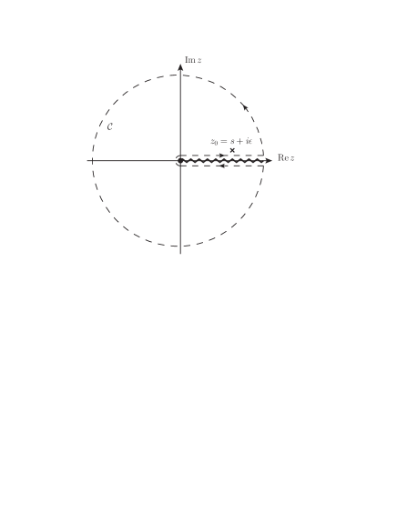
Figure 1: Integration contour for using Cauchy’s integral theorem for a function that has a branch cut along the positive real axis (indicted by a zigzag line). The circle section is understood to have a radius $R\to\infty$.

Derivation of eq. (27): Suppose a function $f(z),\,z\in\mathbbm{C}$ has a branch cut along the positive real axis, but is analytical elsewhere. One can then apply Cauchy’s integral theorem for a contour $\cal C$ that excludes the branch cut, see Fig. 1

$$f(z_{0})=\frac{1}{2\pi i}\oint_{\cal C}dz^{\prime}\;\frac{f(z^{\prime})}{z^{\prime}-z_{0}}$$ (28)

If $f(z)$ vanishes sufficiently fast for $|z|\to\infty$, only the parts of $\cal C$ along the real axis need to be considered. For $z_{0}=s+i\epsilon$ one then obtains

$$f(s+i\epsilon)=\frac{1}{2\pi i}\int_{0}^{\infty}ds^{\prime}\;\frac{f(s^{\prime}+i\delta)-f(s^{\prime}-i\delta)}{s^{\prime}-s-i\epsilon}$$ (29)

where $\delta<\epsilon$ are both infinitesimally small. Applying this to $f(z)=\Pi(z)$ and noting that $\Pi(s^{\prime}-i\delta)=\Pi^{*}(s^{\prime}+i\delta)$,

$$\text{Re}\,\Pi(s)=\frac{1}{\pi}\int_{0}^{\infty}ds^{\prime}\;\frac{\text{Im}\,\Pi(s^{\prime}+i\delta)}{s^{\prime}-s-i\epsilon}$$ (30)

[The $i\epsilon$ on the l.h.s. can be dropped if we only consider the real part of $\Pi$.]

Now we can relative the photon vacuum polarization $\Pi(s)$ to the matrix element for $e^{+}e^{-}\to e^{+}e^{-}$ with a photon self-energy in the s-channel:

$$\text{Im}\,\Pi(s^{\prime}) =\frac{1}{e^{2}}\;\;\text{Im}\;{\cal M}\biggl{\{}\raisebox{-6.99997pt}{\psfig{height=20.00003pt}}\biggr{\}}_{\theta=0}$$ (31)

$$=\frac{s^{\prime}}{e^{2}}\sum_{f}\sigma[e^{+}e^{-}\to f\bar{f}]$$ [optical theorem] (32)

$$=\frac{s^{\prime}}{e^{2}}\,R(s^{\prime})\,\underbrace{\sigma[e^{+}e^{-}\to\mu^{+}\mu^{-}]}_{4\pi\alpha^{2}/(3s^{\prime})}$$ (33)

where “$\theta=0$” indicates that we are restricting ourselves to forward scattering, $i.\,e.$ the kinematics of the final-state $e^{+}e^{-}$ are the same as in the initial state. Then we can apply the optical theorem in (32). Inserting (33) into (30), one arrives at

$$\text{Re}\;\bigl{[}\Pi(s)-\Pi(0)\bigr{]}=\frac{\alpha}{3\pi}\int_{0}^{\infty}ds^{\prime}\;R(s^{\prime})\biggl{[}\frac{1}{s^{\prime}-s-i\epsilon}-\frac{1}{s^{\prime}}\biggr{]}$$ (34)

which immediately leads to the formula for $\Delta\alpha$ in (27).  

Exercise:

Compute the result in (24). Hint: $\Sigma_{T}(k^{2})$ can be computed with Feynman rules and standard techniques, with the result $\frac{\alpha}{3\pi}\Bigl{[}\frac{3(d/2-1)k^{2}+6m^{2}}{d-1}B_{0}(k^{2},m^{2},m^{2})-\frac{4(d-2)}{d-1}A_{0}(m^{2})\Bigr{]}$. To compute the derivative of $B_{0}(k^{2},m^{2},m^{2})$, show that $\frac{\partial^{2}}{\partial k_{\mu}\partial k^{\mu}}f(k^{2})=4k^{2}\,f^{\prime\prime}(k^{2})+2d\,f^{\prime}(k^{2})$. Then apply $\frac{\partial^{2}}{\partial k_{\mu}\partial k^{\mu}}$ inside the integral and use this to compute $\frac{\partial}{\partial(k^{2})}B_{0}(k^{2},m^{2},m^{2})\big{|}_{k^{2}=0}$. Finally, express the result in terms of $A_{0}(m^{2})$ and derivatives thereof and use $A_{0}(m^{2})=m^{2}\Bigl{[}\frac{2}{4-d}-\gamma_{E}-\ln\frac{m^{2}}{4\pi\mu^{2}}+1\Bigr{]}.$

2.2 On-shell Renormalization in the Standard Model

In this subsection, the renormalization procedures from QED are extended to the full Standard Model (SM). Some unique aspects related to electroweak symmetry breaking and massive gauge bosons are reviewed in detail, whereas the remainig aspects that are conceptually similar to QED are only summarized briefly.

Gluon	$G_{0}^{a}=\sqrt{1+\delta Z_{G}}\,G^{a}\quad[a=1,...8]$
Charged $W^{\pm}$ bosons	$W_{0}^{\pm}=\sqrt{1+\delta Z_{W}}\,W^{\pm}$
Photon, $Z$ boson	$\begin{pmatrix}Z_{0}\\[-2.15277pt] A_{0}\end{pmatrix}=\begin{pmatrix}\sqrt{1+\delta Z_{ZZ}}&\frac{1}{2}\delta Z_{AZ}\\[-2.15277pt] \frac{1}{2}\delta Z_{AZ}&\sqrt{1+\delta Z_{AA}}\end{pmatrix}\begin{pmatrix}Z\\[-2.15277pt] A\end{pmatrix}$
Higgs boson	$H_{0}=\sqrt{1+\delta Z_{H}}\,H$
Fermions	$\begin{matrix}\psi^{L}_{f,0}=\sqrt{1+\delta Z^{L}_{f}}\,\psi^{L}_{f}\\ \psi^{R}_{f,0}=\sqrt{1+\delta Z^{R}_{f}}\,\psi^{R}_{f}\end{matrix}$

Table 1: Field renormalization counterterms of the SM fields.

The field content of the SM and the associated field renormalization counterterms are listed in Tab. 1. The photon and $Z$ boson receive a matrix-valued renormalization factor to account for mixing between these two fields. Since the left- and right-handed fermions in the SM have different interactions, the also receive independent renormalization factors.

In addition to the field renormalization terms, the SM also contains several parameters that in general will be renormalized by higher-order effects:

• Gauge couplings $g,g^{\prime},g_{\rm s}$ associated with the U(1), SU(2) and SU(3) gauge interactions.

• Yukawa couplings $y_{f}$. In general these are matrices in the space of the three SM fermion generations, but for the purpose of these lecture we will ignore CKM mixing.

• Higgs vacuum expectation value (vev) $v=\langle\phi_{2}\rangle\approx 246$ GeV, where $\phi$ is the Higgs SU(2) doublet, and the Higgs self-coupling $\lambda$.

For the renormalizion procedure, it is desirable to relate these parameters to observables, such as

• the positron charge $e$ (in the Thomson limit);

• the massive boson masses $M_{W},\,M_{Z},\,M_{H}$;

• the fermion masses $m_{f}$ ($f=e,\mu,\tau,u,d,s,c,b,t$).

At tree-level, the relationship between parameters and these observables is given by the following equations

$$\hskip 12.91663pt\begin{aligned} &\bullet\;c_{\scriptscriptstyle{\mathrm{W}}}\equiv\cos\theta_{\rm W}=\frac{M_{W}}{M_{Z}},\quad s_{\scriptscriptstyle{\mathrm{W}}}^{2}=1-c_{\scriptscriptstyle{\mathrm{W}}}^{2},\\ &\bullet\;g=\frac{e}{s_{\scriptscriptstyle{\mathrm{W}}}},\quad g^{\prime}=\frac{e}{c_{\scriptscriptstyle{\mathrm{W}}}},\\ &\bullet\;v=2M_{W}/g,\\ &\bullet\;\lambda=M_{H}^{2}/(2v^{2}).\end{aligned}$$ (35)

Here the weak mixing angle $\theta_{\rm W}$ has been introduced for convenience.

The on-shell (OS) renormalization scheme is defined by enforcing relations in eq. (35) to all orders in perturbation theory.

Note the absence of $g_{\rm s}$ in this list. Since the strong coupling becomes non-perturbative at low energies, there is no OS definition for $g_{\rm s}$. Instead, the most common prescription for this coupling is the so-called $\overline{{\mathrm{MS}}}$ scheme, where the counterterm is defined as a pure UV-divergent term in dimensional regularization:

$$\delta g_{\rm s} =(4\pi e^{-\gamma_{\rm E}})^{L\varepsilon}\Bigl{(}\frac{C_{L}}{\varepsilon^{L}}+\frac{C_{L-1}}{\varepsilon^{L-1}}+...+\frac{C_{1}}{\varepsilon}\Bigr{)}, \varepsilon=\frac{2}{4-d},\quad L=\text{loop order}$$ (36)

where the $C_{i}$ are chosen such that the sum of the $L$-loop corrections to the $gq\bar{q}$ vertex and the vertex counterterm are UV-finite:

$$\left[\raisebox{-20.00003pt}{\psfig{height=45.00006pt,bb=240 640 350 720,clip={}}}\right]_{L\rm-loop}+\raisebox{-20.00003pt}{\psfig{height=45.00006pt,bb=240 640 350 720,clip={}}}\times\bigl{[}\sqrt{1+\delta Z_{G}}\,(1+\delta Z_{q})(1+\delta g_{\rm s})\bigr{]}_{L\rm-loop}=\text{finite}$$ (37)

$\gamma$–$Z$ mixing:

The derivation of the OS counterterms proceeds in a similar fashion as for QED, with a few modifications. For example, the expression for the charge counterterm in (23) must be adjusted to account for photon–$Z$ mixing:

$$\delta Z_{e(1)} =-\tfrac{1}{2}\delta Z_{AA(1)}-\frac{s_{\scriptscriptstyle{\mathrm{W}}}}{2c_{\scriptscriptstyle{\mathrm{W}}}}\delta Z_{ZA(1)}$$ (38)

Here and the in the following the subcript $(n)$ indicates the loop order.

Additional renormalization conditions are needed to fix the mixing counterterms $\delta Z_{ZA}$ and $\delta Z_{AZ}$. Within the OS scheme, this is achieved by demanding that an on-shell photon does not mix with the $Z$ boson, and conversly an on-shell $Z$ boson does not mix with the photon. At one-loop order, we can write the photon–$Z$ two-point function as

$$G_{\mu\nu(1)}^{AZ} \equiv\;\raisebox{-13.00005pt}{\psfig{height=30.00005pt,bb=90 640 510 720,clip={}}}$$

$$=-i\Bigl{(}g_{\mu\nu}-\frac{k_{\mu}k_{\nu}}{k^{2}}\Bigr{)}\bigl{[}\Sigma^{AZ}_{T(1)}(k^{2})+k^{2}\tfrac{1}{2}\delta Z_{AZ(1)}+(k^{2}-M_{Z}^{2})\tfrac{1}{2}\delta Z_{ZA(1)}\bigr{]}-i\frac{k_{\mu}k_{\nu}}{k^{2}}\bigl{[}...\bigr{]}$$ (39)

where the blob symbolizes all loop diagrams contributing at the given order, whereas the cross symbolizes the counterterm contributions. The former is formally described by the photon–$Z$ self-energy $\Sigma^{AZ}_{T(1)}$, whereas the latter receives two contributions: the one with $\delta Z_{AZ(1)}$ stems from the $A_{0}$ propagator, when the $A_{0}$ field then gets renormalized according to Tab. 1, while the one with $\delta Z_{ZA(1)}$ stems from the $Z_{0}$ propagator, when the $Z_{0}$ field gets renormalized. The longitudinal part has not been spelled out in (39) because it does not contribute to physical in- and out-states. Now, imposing the on-shell non-mixing conditions, one obtains

$$G_{\mu\nu(1)}^{AZ}=0\quad\text{for }k^{2}=0 \Rightarrow\quad\delta Z_{ZA(1)} =2\frac{\Sigma^{AZ}_{T(1)}(0)}{M_{Z}^{2}}$$ (40)

$$G_{\mu\nu(1)}^{AZ}=0\quad\text{for }k^{2}=M_{Z}^{2} \Rightarrow\quad\delta Z_{AZ(1)} =-2\frac{\text{Re}\,\Sigma^{AZ}_{T(1)}(M_{Z}^{2})}{M_{Z}^{2}}$$ (41)

Unstable particles:

An additional complication arises for the renormalization of unstable particles, since their self-energy has an imaginary part, $\text{Im}\,\Sigma(M^{2})>0$, so that the pole of the propagator becomes complex! In practice, in the SM, this is relevant for the $W$ and $Z$ bosons and the top quark, since the width of all other SM particles is negligibly small.

A detailed review of this issue can be found, $e.\,g.$, in Ref. [22]. Here we will illustrate the main points for the example of the $W$ boson to discuss this issue. The propagator pole is defined by

$$Z_{W}(k^{2}-M^{2}_{W,0})+\Sigma^{W}_{T}(k^{2})=0\qquad\text{for}\quad k^{2}=M_{W}^{2}-iM_{W}\Gamma_{W}$$ (42)

The real part of the complex pole can be interpreted as the renormalized mass $M_{W}$, whereas the imaginary part is associated with the decay width, $\Gamma_{W}$. Defining the OS mass in this way ensures that it is well-defined and gauge-invariant to all orders in perturbation theory, since the propagator pole is an analytic property of the physical $S$-matrix [23, 24, 25, 26].

What is the implication of the complex pole for the counterterms $\delta Z_{W}$ and $\delta M_{W}^{2}$? To answer this question, let us assume that $\Gamma_{W}\ll M_{W}$. Then one can expand (42) as

$$Z_{W}(M_{W}^{2}-iM_{W}\Gamma_{W}-M_{W}^{2}-\delta M_{W}^{2})+\Sigma^{W}_{T}(M_{W}^{2})-iM_{W}\Gamma_{W}\,\Sigma^{W\prime}_{T}(M_{W}^{2})+{\cal O}(\Gamma_{W}^{2})=0$$ (43)

where $\Sigma^{W\prime}_{T}(k^{2})=\frac{\partial}{\partial(k^{2})}\Sigma^{W}_{T}(k^{2})$. Taking the imaginary part of (43) one obtains

$$Z_{W}M_{W}\Gamma_{W}\approx\text{Im}\,\Sigma^{W}_{T}(M_{W}^{2})-M_{W}\Gamma_{W}\;\text{Re}\,\Sigma^{W\prime}_{T}(M_{W}^{2})$$ (44)

$$\Rightarrow\quad\Gamma_{W}\approx\frac{\text{Im}\,\Sigma^{W}_{T}(M_{W}^{2})}{M_{W}[Z_{W}+\text{Re}\,\Sigma^{W\prime}_{T}(M_{W}^{2})]}$$ (45)

$$i.\,e.$$ this provides a prescription for computing the total decay width. On the other hand, the real part of (43) leads to

$$Z_{W}\,\delta M_{W}^{2}\approx\text{Re}\,\Sigma^{W}_{T}(M_{W}^{2})+M_{W}\Gamma_{W}\;\text{Im}\,\Sigma^{W\prime}_{T}(M_{W}^{2})$$ (46)

The last term in (46) would not be present for a stable particle. However, for an unstable particle, its inclusion is important to ensure that the renormalized mass is well-defined and gauge-invariant.

Eqs. (45) and (46) depend on the field renormalization counterterm $\delta Z_{W}$. However, it becomes ill-defined when taking into account the width $\Gamma_{W}$, because we do not know whether we should demand that it compensates the self-energy correction for $p^{2}=M_{W}^{2}$ or for $p^{2}=M_{W}^{2}-iM_{W}\Gamma_{W}$. The latter may seem preferrable because it is the gauge-invariant pole of the propagator, but what are we to make of an external particle with complex momentum?

The problem occurs because we have explicitly taken into account the fact that the $W$ boson is unstable. But in this case it cannot be an asymptotic external state, because it will decay rather rapidly! Instead, we should consider a process where the production and decay of the $W$ boson is included, so that it occurs only as an internal particle. An example would be $u\bar{d}\to W^{+}\to\mu^{+}\nu_{\mu}$. When computing this process, $\delta Z_{W}$ occurs in the intermediate $W$ propagator, but also in the initial-state $u\bar{d}W$ vertex and in the final-state $W\mu^{+}\nu_{\mu}$ vertex. Summing up all these contributions, one can easily verify that $\delta Z_{W}$ drops out in the total result, and we never need to provide an explicit expression for it.

Tadpole renormalization:

A large number of loop diagrams contains so-called tadpoles, which are sub-diagrams with one external leg. An example for the process $\mu^{-}\to e^{-}\nu_{\mu}\bar{\nu}_{e}$ is shown to the right. In a practical calculation, these diagrams constitute a large fraction of the total number of diagrams and they signficantly increase the size of intermediate algebraic expressions.

Fortunately, these tadpoles can be absorbed by renormalizing the Higgs vev,

$$v_{0}=v+\delta v$$ (47)

Introducing this additional counterterm will break any tree-level relationships between the vev and other parameters. For example, for the bare Higgs potential,

$$V_{0} =-\mu_{0}|\phi|^{2}+\lambda_{0}|\phi|^{4}$$ (48)

one has $v_{0}=\sqrt{\mu_{0}^{2}/\lambda_{0}}$, but this relationship between $v$, $\lambda$ and $\mu$ can be modified at higher orders without causing any problems since $v$ is not an observable, and its numerical value does not have any direct physical meaning. Therefore, we are free to choose the counterterm $\delta v$ at will during the computation of any physical observables, without affecting the final result.

To see how this can be used to eliminate tadpole diagrams, let us write the Higgs doublet field as

$$\phi =\begin{pmatrix}G^{+}\\ \frac{1}{\sqrt{2}}(v+H+G^{0})\end{pmatrix}$$ (49)

where $G^{+},G^{0}$ are the Goldstone fields. Using $\mu_{0}^{2}=\frac{1}{2}M_{H,0}^{2}=\frac{1}{2}(M_{H}^{2}+\delta\tilde{M}_{H}^{2})$, and expanding the bare Higgs potential to one-loop order, one finds

$$V_{0} =V+\delta V+{\cal O}(\delta X^{2}),$$ (50)

$$V =-\frac{M_{H}^{2}}{2}|\phi|^{2}+\frac{M_{H}^{2}}{2v^{2}}|\phi|^{4},$$ (51)

$$\delta V =\text{const.}-\underbrace{M_{H}^{2}\,\delta v}_{\equiv\,\delta t}\,H+\underbrace{\Bigl{(}\frac{\delta\tilde{M}_{H}^{2}}{2}-\frac{3}{2}M_{H}^{2}\,\frac{\delta v}{v}\Bigr{)}}_{\equiv\,\delta M_{H}^{2}/2}H^{2}-\frac{M_{H}^{2}\,\delta v}{2v}(G_{0}^{2}+2G^{+}G^{-})+\text{interact.}$$ (52)

To avoid clutter, the constant term (which is physically irrelevant) and any interaction terms involving three or more scalar fields have not been spelled out in eq. (52). The term linear in $H$ produces a tadpole-like counterterm Feynman rule:

$$\raisebox{-10.00002pt}{\psfig{width=50.00008pt,bb=245 662 360 712,clip={}}}=i\,\delta t$$ (53)

Now one can choose $$\delta t \delta v$$ (or, equivalently, ) such that the sum of the tadpole loop diagrams plus this counterterm vanishes:

$$\raisebox{-10.00002pt}{\psfig{width=50.00008pt,bb=245 662 360 712,clip={}}}\;+\raisebox{-10.00002pt}{\psfig{width=50.00008pt,bb=245 662 360 712,clip={}}}\;=\;0$$ (54)

When adopting this convention, no tadpole diagrams need to be taken into account in an actual calculation of a physics process.

As can be seen in (52), $\delta v$ also modifies the Higgs mass counterterm, but this shift can be absorbed by redefining this mass counterterm. The new counterterm $\delta M_{H}^{2}$ can be derived from the standard OS renormalization condition without needing to worry about tadpoles.

However, $\delta v$ also generates a fictious mass for the Goldstone bosons ($G^{0},G^{\pm}$), as also shown in (52). Since these fields are a priori massless, this fictious mass cannot be absorbed by any redefinition of other parameters. While this is not explicitly shown in (52), additional non-trivial contributions proportional to $\delta v$ also appear in self-interactions of the Goldstone scalars. These Goldstone mass and vertex corrections are a (small) price to pay for renormalizing away the tadpole diagrams. For a complete list of Feynman rules modified by $\delta t$ ($\delta v$), see $e.\,g.$ Ref. [21].

Exercise:

Determine the contributions of $\delta t$ and $\delta M_{H}^{2}$ to the scalar three- and four-point interactions in $\delta V$.

2.3 Other Renormalization Schemes

While the OS scheme has certain advantages, by relating renormalized SM parameters to physical observables, a range of other renormalization schemes are frequently adopted in the literature. They each come with specific advantage and disadvantages (indicated by +$\bigcirc$ and $-$$\bigcirc$ below, respectively).

$\overline{{\mathrm{MS}}}$ scheme:

All already mentioned on page 1, all counterterms in the $\overline{{\mathrm{MS}}}$ scheme have the form

$$\delta X =(4\pi e^{-\gamma_{\rm E}})^{L\varepsilon}\Bigl{(}\frac{C_{L}}{\varepsilon^{L}}+\frac{C_{L-1}}{\varepsilon^{L-1}}+...+\frac{C_{1}}{\varepsilon}\Bigr{)}, \varepsilon=\frac{2}{4-d},\quad L=\text{loop order}$$ (55)

$i.\,e.$ they simply subtract the divergent pieces of an amplitude but do not contain any non-trivial finite terms. The factor with $4\pi$ and $\gamma_{\rm E}$ in front is included to cancel similar terms that universally appear for any divergent loop integral in dimensional regularization.

• The dependence on the scale $\mu$ of dimensional regularization, $d^{4}k\to\mu^{4-d}d^{d}k$, is not cancelled by the counterterms, so that the $\overline{{\mathrm{MS}}}$ couplings and masses depend on the choice of $\mu$. The $\mu$-dependence can be described by the renormalization group, which allows one to resum dominant terms in some calculations and to study phase transitions.

• In some cases, when renormalizing the relevant parameters of a physical process in the $\overline{{\mathrm{MS}}}$ scheme, the perturbation series for this process converges better than in the OS scheme.

• One needs an additional calculation to relate a $\overline{{\mathrm{MS}}}$ parameter to an oservable, in order to determine the numerical value for this parameter from experiment.

(a)	(b)	(c)	(d)

Figure 2: Diagrams for muon decay (a) in the Fermi model, (b) at tree-level in the SM, and (c,d) contributing to the one-loop corrections in the SM.

$G_{\mu}$ scheme:

The Fermi constant $G_{\mu}$ describes the decay of muons as an effective four-fermion interaction described by the Lagrangian

$${\cal L}_{\rm Fermi}=\frac{G_{\mu}}{2\sqrt{2}}\bigl{(}\overline{\psi}_{\nu_{\mu}}\gamma_{\lambda}\omega_{-}\psi_{\mu}\bigr{)}\bigl{(}\overline{\psi}_{e}\gamma_{\lambda}\omega_{-}\psi_{\nu_{e}}\bigr{)}$$ (56)

where $\omega_{-}\equiv(1-\gamma_{5})/2$. In Feynman diagrammatic form, the muon decay process generated by this interaction in shown in Fig. 2 (a). In the SM, the four-fermion interaction is instead mediated by $W$-boson exchange at tree-level, see Fig. 2 (b). Therefore, $G_{\mu}$ can be expressed in terms of SM parameters,

$$\frac{G_{\mu}}{\sqrt{2}}=\frac{g^{2}}{8M_{W}^{2}}(1+\Delta r)$$ (57)

where $\Delta r$ accounts for corrections beyond tree-level (see Fig. 2 (c,d) for example diagrams). This relation can be used to express the weak coupling $g$ in terms of $G_{\mu}$:

$$g^{2}=4\sqrt{2}\,g_{\mu}M_{W}^{2}(1+\Delta)^{-1}$$ (58)

When computing electroweak radiative corrections, instead of writing them as a series in powers of $g=e/s_{\scriptscriptstyle{\mathrm{W}}}$, one can employ (58) to represent them as a series in powers of $G_{\mu}$.

• $G_{\mu}=1.1663787(6)\times 10^{-5}\,\text{GeV}^{-2}$ is precisely known from measurement [27].

• The leading corrections in $\Delta r$ may (partially) cancel similar terms in other observables. For example, when computing the $W$ decay rate, the one-loop corrections are much smaller in the $G_{\mu}$ scheme than in the OS scheme of the previous subsection [21].

• One needs to include the corrections to muon decay ($\Delta r$) in the calculation of any other observable.

3 Electroweak Precision Observables

The term electroweak precision observable (EWPO) refers to a set of quantities that have been measured with high precision (typically at the per-mille level or better) and that are related to properties of the electroweak ($W$ and $Z$) gauge bosons. In general, they also include a number of quantities that are not stricty instrinsic to the electroweak sector, but that are needed to make predictions for EWPOs within the SM. These are often called “input parameters.”

Another rationale for distinguishing between input parameters and “genuine” EWPOs is the expectation that input parameters are unlikely to be significantly affected by new physics beyond the SM (possible reasons include: their measurement is based on kinematical features; they are protected by symmetries; new physics decouples due to effective field theory arguments). On the other hand, the genuine EWPOs can get modified by a large range of beyond-the-SM (BSM) models. In fact, one of the main motiviations for studying EWPOs is their potential to constrain new physics by comparing measurement data with theoretical SM predictions.

In the following subsection, the relevant input parameters will be discussed one by one, before giving an overview of the most important genuine EWPOs in the remainder of this chapter.

3.1 Input Parameters

A typical choice of input parameters for electroweak precision studies is: $\alpha=\frac{e^{2}}{4\pi}$, $G_{\mu}$, $\alpha_{\rm s}$, $M_{Z}$, $M_{H}$, $m_{t}$. The masses of any fermions besides the top quark ($m_{f},\,f\neq t$) are generally negligible in electroweak physics since their impact is suppressed by powers of $m_{f}^{2}/M_{W}^{2}$, with the exception of $\Delta\alpha$, where they contribute logarithmically, see page 2.1.

Fine structure constant $\alpha$:

There are two leading methods for determining the value of $\alpha$:

• From the electron magnetic moment $a_{e}=\frac{g_{e}-2}{2}$ [28], which has been theoretically computed to very high precision:

  $$a_{e}=\frac{\alpha}{2\pi}+A_{2}\alpha^{2}+A_{3}\alpha^{3}+A_{4}\alpha^{4}+A_{5}\alpha^{5}+C_{\rm EW}\frac{m_{e}^{2}}{M_{W}^{2}}+C_{\rm had}\frac{m_{e}^{2}}{\Lambda_{\rm QCD}^{2}}...$$ (59)

  The coefficients $A_{i}$ denote $i$-loop QED loop corrections, which have been computed to five-loop order [29, 30, 31]. Electroweak corrections, denoted by the term with $C_{\rm EW}$, are suppressed by the small electron mass. Similarly, hadronic corrections, denoted by the term with $C_{\rm had}$, first enter at the two-loop level, and they are suppressed by the ratio $m_{e}^{2}/\Lambda_{\rm QCD}^{2}$, with $\Lambda_{\rm QCD}\sim{\cal O}(1\,\text{GeV})$. Both of these contributions are negligible at current levels of precision.

  Comparing (59) to precise measurements of $g_{e}$ using Penning traps [32], one finds [33, 34]

  $$\alpha^{-1}=137.035\,999\,174(35)$$ (60)

  where the numbers in brackets indicate the uncertainty in the last quoted digits.

• An independent determination of $\alpha$ can be obtained from the defining formula for the Rydberg constant, $R_{\infty}$:

  $$\alpha^{2}=\frac{R_{\infty}}{2c}\,\frac{m_{\rm At}}{m_{e}}\,\frac{h}{m_{\rm At}}$$ (61)

  Here $m_{\rm At}$ is the mass of some atom. The fine structure constant can be determined by using precise values for $R_{\infty}$ (from atomic spectroscopy), $m_{\rm At}$ and $m_{e}$ (in atomic units), and $h/m_{\rm At}$ (from atom interferometry). The limiting factor, in terms of precision, is the measurement of $h/m_{\rm At}$, which recently has been significantly improved for Cs-133 atoms [35], resulting in

  $$\alpha^{-1}=137.035\,999\,046(27)$$ (62)

The two values (60) and (62) exhibit a 2.5$\sigma$ tension.

Fermi constant $G_{\mu}$:

As already mentioned in section 2.3, the Fermi constant gives the strength of an effective four-fermion interaction, which can be extracted from muon decay. Besides the leading-order diagram in Fig. 3 (a), there are also significant QED corrections as illustrated in Fig. 3 (b,c). The corrections are known to next-to-next-to-leading (NNLO) order [36, 37, 38]. Combining these with the measured value of the muon lifetime, $\tau_{\mu}$, [39], one obtains

$$G_{\mu}=1.1663787(6)\times 10^{-5}\mbox{ GeV}^{-2}$$ (63)

where the uncertainty is dominant by the experimental measurement of $\tau_{\mu}$, whereas the estimated theory error from missing higher orders is sub-dominant.

(a)	(b)	(c)

Figure 3: Muon decay in the Fermi model: (a) leading order diagram, and sample diagrams for the (b) one-loop and (c) two-loop QED corrections.

Strong coupling $\alpha_{\rm s}=g_{\rm s}^{2}/(4\pi)$:

There are many independent methods for its determination. For a complete review, see chapter 9 of Ref. [27]. In the following, a few of the most precise methods are listed:

• The currently most precise approach uses lattice QCD calculations. Two recent studies yield

  $$\text{Lattice:}\qquad\alpha_{\rm s} =0.1185\pm 0.0008\quad\text{\cite[cite]{[\@@bibref{Number}{Bruno:2017gxd}{}{}]}}$$ (64)

  $$\alpha_{\rm s} =0.1172\pm 0.0011\quad\text{\cite[cite]{[\@@bibref{Number}{Zafeiropoulos:2019flq}{}{}]}}$$ (65)

• Differential distributions (event shapes) of $e^{+}e^{-}\to\text{jets}$ and deep inelastic scattering (DIS), using NNLO QCD corrections. These approaches yield values of $\alpha_{\rm s}\approx 0.114$ on average, significantly below the numbers obtained with other methods. Possible issues include large non-perturbative QCD uncertainties (for $e^{+}e^{-}\to\text{jets}$) and scheme dependence and parametrization of parton distribution functions (for DIS). See chapter 9 of Ref. [27] for more details.

• From the branching fraction of taus into hadrons one obtains

  $$\tau\text{ decays:}\qquad\alpha_{\rm s} =0.117\pm 0.002$$ (66)

  (see section 10 of Ref. [27]). This determination is subject to non-perturbative hadronic uncertainties, $e.\,g.$ from violations of quark-hadron duality.

• EWPOs, in particular the branching ratio $R_{\ell}\equiv\Gamma[Z\to\text{had.}]/\Gamma[Z\to\ell^{+}\ell^{-}]$ ($\ell=e,\mu,\tau$), yield

  $$\text{Electroweak precision:}\qquad\alpha_{\rm s} =0.1221\pm 0.0027$$ (67)

  (see section 10 of Ref. [27]). This method has negligible QCD uncertainties (both perturbative and non-perturbative), but since $R_{\ell}$ is a high-energy observable, it is more likely to be impacted by new physics beyond the SM.

Top-quark mass $m_{t}$:

The currently most precise measurements are based on the invariant mass distribution ($m_{\rm inv}$) of the top decay products at LHC (for a review see the section “Top Quark” in Ref. [27]). This approach yields a result that is numerically very close to the OS (pole) mass [42]. However, the OS mass of the top quark is theoretically not well-defined due to the presence of non-perturbative QCD contributions to the top-quark self-energy in (7). These effects, called renormalons, are typically of the order of ${\cal O}(\Lambda_{\rm QCD})\sim 300$ MeV, where $\Lambda_{\rm QCD}$ is the scale where $\alpha_{\rm s}$ becomes non-perturbative [43]. Therefore, when trying to use the peak of the $m_{\rm inv}$ distribution as an input for other calculations, there necessarily is an ambiguity of the same order.

The problem of the top-quark mass definition can be circumvented by measuring a more inclusive observable, such as the total $t\bar{t}$ cross-section, $\sigma_{t\bar{t}}$, at the LHC. $\sigma_{t\bar{t}}$ can be described in terms of the $\overline{{\mathrm{MS}}}$ mass $m_{t}^{\overline{{\mathrm{MS}}}}$, which is free of the renormalon ambiguity. However, it may be affected by possible new physics effects, such as heavy new physics particles in the $s$-channel, which are predicted by theories with extra dimensions and other models (see Fig. 4).

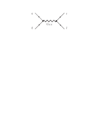
Figure 4: Example of a new physics contribution to $t\bar{t}$ production at the LHC, due to a Kaluza-Klein excitation of the gluon.

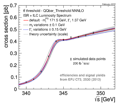
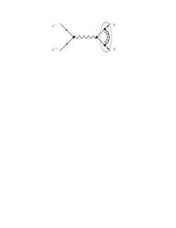
(a)	(b)

Figure 5: (a) Illustration of a 10-point threshold scan for $e^{+}e^{-}\to t\bar{t}$ at ILC (figure taken from Ref. [44]). (b) Sample diagram of a gluon-exchange contribution to the $t\bar{t}$ bound-state effect near threshold.

At future $e^{+}e^{-}$ colliders with a center-of-mass energy of at least 350 GeV, a precise, well-defined measurement of $m_{t}$ can be performed, that is largely unaffected by BSM physics. This is achieved through a threshold scan, measuring $\sigma_{t\bar{t}}$ at different values of the center-of-mass energy $\sqrt{s}$, see Fig. 5 (a). The shape of $\sigma_{t\bar{t}}$ as a function of $\sqrt{s}$ can be predicted with high precision in terms of $m_{t}^{\overline{{\mathrm{MS}}}}$, including NNNLO QCD as well as NLO and leading NNLO electroweak corrections [45, 46]. The small bump in the lineshape at the threshold is caused by 1S bound-state effects from gluon exchange, as illustrated in Fig. 5 (b). Note that this is not a true bound state since the decay width of the top quark is larger than the binding energy, but it still leads to a an enhancement of the cross-section at the would-be bound-state energy.

Z-boson mass $M_{Z}$:

The most precise determination of $M_{Z}$ is obtained from measurements of the cross-section for $e^{+}e^{-}\to f\bar{f}$ at different center-of-mass energies at LEP.

Ignoring $\gamma$–$Z$ mixing for the moment, this process can be described by the generic Feynman diagram below, yielding

$$\sigma_{f}(s) =\biggl{|}\frac{\color[rgb]{0,0,1}R(s)}{s-M_{Z}^{2}-\color[rgb]{1,0,0}\delta M_{Z}^{2}+\Sigma^{Z}_{T}(s)/Z_{ZZ}}\biggr{|}^{2}$$ (68)

$$=\biggl{|}\frac{R(M_{Z}^{2})}{s-M_{Z}^{2}+iM_{Z}\Gamma_{Z}}+\text{non-res.}\biggr{|}^{2}$$ (69)

In line (68), the red blob and terms indicates the contribution from the Z self-energy (including counterterms), whereas the blue blobs and term denotes contributions from vertex corrections. The amplitude inside the modulus brackets $||$ in (68) has a complex pole (see page 2.2). Expanding about this pole and using $\Gamma_{Z}\ll M_{Z}$ yields the expression in (69), which has a resonant piece and an infinite series of terms suppressed by powers of $(s-M_{Z}^{2})$ and $\Gamma_{Z}/M_{Z}$, which are not explicitly spelled out here.

Including $\gamma$–$Z$ mixing requires the replacement of $\Sigma_{T}^{Z}(s)$ with

$$\Sigma_{T}^{Z}(s) \to\Sigma_{T}^{Z}(s)-\frac{[\hat{\Sigma}_{T}^{AZ}(s)]^{2}}{s+\hat{\Sigma}_{T}^{A}(s)}\,,$$ (70)

$$\hat{\Sigma}_{T}^{AZ}(s) =\Sigma_{T}^{AZ}(s)+\tfrac{1}{2}\delta Z_{ZA}\sqrt{Z_{ZZ}}(s-M_{Z}^{2}-\delta M_{Z}^{2})+s\tfrac{1}{2}\delta Z_{AZ}\sqrt{Z_{AA}}\,,$$ (71)

$$\hat{\Sigma}_{T}^{A}(s) =\Sigma_{T}^{A}(s)+s\tfrac{1}{2}\delta Z_{AA}+\tfrac{1}{4}(\delta Z_{ZA})^{2}(s-M_{Z}^{2}-\delta M_{Z}^{2})$$ (72)

Even though the expressions for the counterterms are rather lengthy, the result still takes the general form in (69), since this result only relies on the presence of a complex pole in the amplitude.

Carrying out the square in (69) yields

$$\sigma_{f}(s) =\frac{|R(M_{Z}^{2})|^{2}}{(s-M_{Z}^{2})^{2}+M_{Z}^{2}\Gamma_{Z}^{2}}+\text{non-res.}$$ (73)

which is called a Breit-Wigner resonance, see the solid curve in Fig. 6.

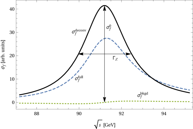
Figure 6: Illustration of $Z$-pole cross-section line-shape (not to scale). The solid (dashed) line indicates the line-shape without (with) initial-state QED radiation. The dotted line depicts backgrounds from photon exchange and box contributions to the cross-section (without initial-state radiation). [Figure taken from Ref. [22].]

By fitting this curve to experimental measurements of $\sigma_{f}$ at three or more values of $\sqrt{s}$, one can determine $M_{Z}$ and $\Gamma_{Z}$ at high precision. However, in the experimental studies at LEP, a different parametrization of the Breit-Wigner resonance has been used,

$$\sigma_{f}(s) =\frac{R^{\prime 2}}{(s-m_{Z}^{2})^{2}+s^{2}\gamma_{Z}^{2}/m_{Z}^{2}}+\text{const.}$$ (74)

with the results [27, 47]

$$m_{Z} =91.1876\pm 0.0021\,\text{GeV}, \gamma_{Z} =2.4942\pm 0.0023\,\text{GeV}$$ (75)

When ignoring the non-resonant terms, the two forms (73) and (74) are fully equivalent, but the mass and width parameters are different. The relation is given by [48]

$$\begin{aligned} M_{Z}&=m_{Z}(1+\gamma_{Z}^{2}/m_{Z}^{2})^{-1/2}\approx m_{Z}-34\,\text{MeV},\\ \Gamma_{Z}&=\gamma_{Z}(1+\gamma_{Z}^{2}/m_{Z}^{2})^{-1/2}\approx m_{Z}-0.9\,\text{MeV}\\ \end{aligned}$$ (76)

Thus, whenever aiming to use (75) as inputs to a theory calculation, one first needs to apply the translation (76).

Exercise:

For each the quantities listed above, which of the following concepts limits the influence of new physics in their determination: measurement is based on kinematical features; protected by symmetries; new physics decouples due to effective field theory arguments (see appendix for answer).

3.2 Z-pole EWPOs

Electroweak precision observables at the $Z$-pole are related to the vector and axial-vector couplings of the $Z$–fermion interactions. For massless fermions, these interactions have the form

$$\overline{\psi}_{f}\,i\gamma_{\mu}(v_{f}-a_{f}\gamma_{5})\,\psi_{f}$$ (77)

where the subscript $f$ labels the fermion type ($f=e,\mu,\tau,...$). At leading order (Born level),

$$v_{f}=e\frac{I^{3}_{f}-2s_{\scriptscriptstyle{\mathrm{W}}}^{2}Q_{f}}{2s_{\scriptscriptstyle{\mathrm{W}}}c_{\scriptscriptstyle{\mathrm{W}}}},\qquad a_{f}e\frac{I^{3}_{f}}{2s_{\scriptscriptstyle{\mathrm{W}}}c_{\scriptscriptstyle{\mathrm{W}}}}$$ (78)

Here $Q_{f}$ is the fermion charge in units of the positron charge $e$, whereas $I^{3}_{f}$ is the third component of weak isospin. Beyond Born level, $v_{f}$ and $a_{f}$ receive radiative corrections within the SM and potentially also from BSM contributions. Therefore, one can use precision measurements of these quantities to constrain and potentially discover various typoes of new physics.

The following observables are useful to extract information about $v_{f}$ and $a_{f}$ from data:

• The total $Z$ decay width, $\Gamma_{Z}$. According to (45), $\Gamma_{Z}\propto\text{Im}\,\Sigma^{W}_{T}(M_{W}^{2})$. Using the optical theorem, which diagrammatically corresponds to cutting the self-energy diagram shown to the right, the width is related to the matrix elements for the process $Z\to f\bar{f}$, so that

  

  $$\Gamma_{Z}\propto\sum_{f}\bigl{|}{\cal M}[Z\to f\bar{f}]\bigr{|}^{2}=\sum_{f}\bigl{(}|v_{f}|^{2}+|a_{f}|^{2}\bigr{)}$$ (79)

• The cross-section for $e^{+}e^{-}\to Z\to f\bar{f}$, which, up to a simple phase-space and flux factor, can be written as

  $$\sigma_{f}(s)\propto\bigl{(}|v_{e}|^{2}+|a_{e}|^{2}\bigr{)}\,\biggl{|}\frac{1}{s-M_{Z}^{2}+iM_{Z}\Gamma_{Z}+\Sigma^{Z}_{T}(s)+...}\biggr{|}^{2}\bigl{(}|v_{f}|^{2}+|a_{f}|^{2}\bigr{)}$$ (80)

  where the dots in the denominator refer to the $\gamma$–$Z$ mixing and counterterms described on page 3.1. Near the $Z$ pole ($s\approx M_{Z}^{2}$) this expression can be recast into the form

  $$\sigma_{f}(s)\approx 12\pi\frac{\Gamma_{e}\Gamma_{f}}{(s-M_{Z}^{2})^{2}+M_{Z}^{2}\Gamma_{Z}^{2}}\equiv\sigma_{f}^{0}$$ (81)

  where $\Gamma_{f}$ is the partial width for the decay $Z\to f\bar{f}$ into a particular fermion type $f$.

• With polarized electron beams, one can measure the cross-section separately for left- and right-handed polarized electrons:

  $$\sigma_{\rm L}\equiv\sigma[e^{+}e^{-}_{\rm L}\to f\bar{f}]\propto|v_{e}+a_{e}|^{2}\,\biggl{|}\frac{1}{s-M_{Z}^{2}+iM_{Z}\Gamma_{Z}}\biggr{|}^{2}\bigl{(}|v_{f}|^{2}+|a_{f}|^{2}\bigr{)}$$ (82)

  $$\sigma_{\rm R}\equiv\sigma[e^{+}e^{-}_{\rm R}\to f\bar{f}]\propto|v_{e}-a_{e}|^{2}\,\biggl{|}\frac{1}{s-M_{Z}^{2}+iM_{Z}\Gamma_{Z}}\biggr{|}^{2}\bigl{(}|v_{f}|^{2}+|a_{f}|^{2}\bigr{)}$$ (83)

  From this one can form a left-right asymmetry where several important systematic uncertainties, such as the lumonisity uncertainty or the detector acceptance, cancel:

  $$A_{\rm LR}=\frac{\sigma_{\rm L}-\sigma_{\rm R}}{\sigma_{\rm L}+\sigma_{\rm R}}=\frac{2\,\text{Re}\{v_{e}a_{e}^{*}\}}{|v_{e}|^{2}+|a_{e}|^{2}}=\frac{2\,\text{Re}\{v_{e}/a_{e}\}}{1+|v_{e}/a_{e}|^{2}}\equiv{\cal A}_{e}$$ (84)

  Thus, in contrast to the decay width or the total cross-section, this asymmetry yields information about the ratio of the vector and axial-vector couplings.

  At Born level: $$\frac{v_{f}}{a_{f}} =1-4|Q_{f}|s_{\scriptscriptstyle{\mathrm{W}}}^{2}\quad\Bigl{[}=1-4s_{\scriptscriptstyle{\mathrm{W}}}^{2}\text{ for }f=e\Bigr{]}$$ (85)

  With higher orders: $$\text{Re}\,\frac{v_{f}}{a_{f}} \equiv 1-4|Q_{f}|\sin^{2}\theta_{\rm eff}^{f}$$ (86)

  where we have defined the effective weak mixing angle $\sin^{2}\theta_{\rm eff}^{f}$ as the radiative corrected verion of the on-shell weak mixing angle $s_{\scriptscriptstyle{\mathrm{W}}}^{2}$.

• Without polarized beams, one can use the differential cross-section to obtain information about the ratio $v_{f}/a_{f}$:

  $$\frac{d\sigma}{d\cos\theta}\propto\bigl{(}|v_{e}|^{2}+|a_{e}|^{2}\bigr{)}\bigl{(}|v_{f}|^{2}+|a_{f}|^{2}\bigr{)}(1+\cos^{2}\theta)+4\,\text{Re}\{v_{e}a_{e}^{*}\}\,\text{Re}\{v_{f}a_{f}^{*}\}\cos\theta$$ (87)

  where we have spelled out only the terms that depend on the scattering angle $\theta$ (the angle between the momenta of the incident $e^{-}$ and the outgoing $f$), whereas all other terms (such as the $Z$ propagator) subsumed in the unspecified proportionality factor.

  The range of possible scattering angle can be divided into a forward and backward hemisphere,

  $$\sigma_{\rm F}\equiv=\int_{0}^{1}d\cos\theta\;\frac{d\sigma}{d\cos\theta}, \sigma_{\rm B}\equiv=\int_{-1}^{0}d\cos\theta\;\frac{d\sigma}{d\cos\theta}$$ (88)

  which then allows us to define the forward-backward asymmetry

  $$A_{\rm FB}^{f}=\frac{\sigma_{\rm F}-\sigma_{\rm B}}{\sigma_{\rm F}+\sigma_{\rm B}}=\frac{3\,\text{Re}\{v_{e}a_{e}^{*}\}\,\text{Re}\{v_{f}a_{f}^{*}\}}{(|v_{e}|^{2}+|a_{e}|^{2})(|v_{f}|^{2}+|a_{f}|^{2}}=\frac{3}{4}{\cal A}_{e}{\cal A}_{f}$$ (89)

The quantities introduced above ($\Gamma_{Z}$, $\Gamma_{f}$, $\sigma^{0}_{f}$, $A_{\rm FB}^{f}$, $A_{\rm LR}$) are so-called pseudo-observables. The reason for this terminology is due to the fact that real observables involve extra effects:

Initial-state radiation (ISR):

There are corrections due to emission of real and virtual photons off the incoming electron and photon. Photons that are soft or collinear to one of the incoming particles lead to contributions that are enhanced by terms involving logarithms of the form

$$\frac{2\alpha}{\pi}L\equiv\frac{2\alpha}{\pi}\ln\frac{s}{m_{e}^{2}}\approx 11\% \text{[for }s=M_{Z}^{2}]$$ (90)

The ISR effects can be taken into account through a convolution

$$\sigma^{\rm full}_{f}(s)=\int_{0}^{1-4m_{f}^{2}/s}dx\;H(x)\,\sigma^{\rm deconv}_{f}\bigl{(}s(1-x)\bigr{)}$$ (91)

The deconvoluted cross-section, $\sigma^{\rm deconv}_{f}$, is illustrated by the gray blows in the diagrams above. The radiator function $H(x)$ contains the soft and collinear photon contributions. It has the general form

$$H(x)=\sum_{n}\Bigl{(}\frac{\alpha}{\pi}\Bigr{)}^{n}\sum_{m=0}^{n}h_{nm}(2L)^{m}$$ (92)

The leading logarithms (for $m=n$) are universal ($i.\,e.$ independent of the specific process) and known to $n=6$ (see Ref. [49] and references therein). Also some sub-leading terms are known for $e^{+}e^{-}\to\gamma^{*}/Z*\to f\bar{f}$. The impact of ISR on the cross-section is shown in Fig. 6.

Backgrounds

: $\sigma^{\rm deconv}_{f}$ receives contributions from several sources:

$$\sigma^{\rm deconv}_{f}=\sigma^{Z}_{f}+\underbrace{\sigma^{\gamma}_{f}+\sigma^{\gamma Z}_{f}+\sigma^{\rm box}_{f}}_{\sigma^{\rm bkgd}_{f}}$$ (93)

where $\sigma_{Z}$ stems from s-channel $Z$-boson exchange, $\sigma_{\gamma}$ from s-channel photon exchange, $\sigma_{\gamma Z}$ from the inteference of these two, and $\sigma_{\rm box}$ from box diagrams that involve the exchange of two (or more) gauge bosons between the initial and final fermions.

Only $\sigma_{Z}$ has a Breit-Wigner resonance at $s\approx M_{Z}^{2}$, whereas the remaining contributions in $\sigma^{\rm bkgd}_{f}$ are relatively suppressed. For measurements near the $Z$ pole, the non-resonant terms in $\sigma^{\rm bkgd}_{f}$ are typically subtracted, using their SM prediction [5].

Detector acceptance and cuts:

The measured cross-section is affected by the capability of the detector to identify the final state $f\bar{f}$ particles, the presence of extra photon radiation in the detector, blind regions of the detector, cuts to suppress backgrounds from fakes, etc. These effects are typically evaluated using Monte-Carlo simulations.

3.2.1 $A_{\rm FB}$ at LHC

In addition to $e^{+}e^{-}$ colliders, EWPOs can also be measured at hardon colliders. However, a challenge arises when trying to determine the forward-backward asymmetry at the LHC from the so-called Drell-Yan process $pp\to\ell^{+}\ell^{-}$ ($\ell=e,\mu$), since the initial state ($pp$) is symmetric and thus there is no obvious distinction between the forward and backward directions.

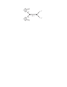
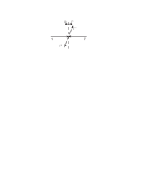
(a)	(b) lab frame	(c) CoM frame

Figure 7: Drell-Yan process at LHC: (a) Leading Feynman diagram; (b) kinematics in the lab frame, and (c) in the center-of-mass frame. The direction of the boost from the center-of-mass to the lab frame is taken at the forward direction to define $A_{\rm FB}$.

However, the leading partonic process consists of an asymmetric quark-antiquark pair, see Fig. 7 (a). On average, the quark momentum is expected to be larger than the antiquark momentum, since the quark may be a valence parton of the proton, whereas the antiquark necessarily stems from the sea parton distribution. Therefore, the final-state $\ell^{+}\ell^{-}$ will typically be boosted in the direction of the incoming quark, Fig. 7 (b). To evaluate $A_{\rm FB}$, the event must be tranformed to the center-of-mass frame, but one can use the boost direction of the event in the lab frame to define the forward direction for the asymmtry, Fig. 7 (c).

Given the large cross-section for $Z$-boson production at the LHC, there is the potential to perfrom high-precision measurements of $A_{\rm FB}$ at the ATLAS and CMS experiments. Nevertheless, the achievable precision is limited by systematic effects:

• The overall boost direction of the event is not a perfect proxy for the direction of the incident quark. To evaluate how often the forward and backward hemispheres get incorrectly assigned, precise parton distribution functions (PDFs) are needed. Thus the measurement precision for $A_{\rm FB}$ is limited by the PDF errors.

• Drell-Yan production receives large QCD corrections from gluon exchange among the initial-state $q\bar{q}$ system. Recently, the NNNLO corrections have been computed [50], but the error from unknown higher-order QCD contribution is still not negligible.

Let us conclude this section by highlighting some examples of EWPO measurements. The best measurement of the total $Z$ width has been obtained at LEP [5]:

$$\Gamma_{Z} =2495.5\pm 2.3\,\text{MeV}$$ (LEP) (94)

For the leptonic effective weak mixing angle, a number different measurements of left-right and forward-backward asymmetries at lepton and hadron colliders are similarly competitive [5, 51, 52]:

$$\sin^{2}\theta_{\rm eff}^{\ell}=\; 0.23098\pm 0.00026 (A_{\rm LR}\text{ @ SLD})$$

$$0.23221\pm 0.00029 (A_{\rm FB}^{b}\text{ @ LEP})$$

$$0.23148\pm 0.00033 (A_{\rm FB}^{e,\mu}\text{ @ TeVatron})$$

$$0.23140\pm 0.00036 (A_{\rm FB}^{e,\mu}\text{ @ ATLAS})$$ (95)

3.3 W-boson mass

The $W$-boson mass is typically not considered an input parameters, since it can be computed from the Fermi constant $G_{\mu}$, using eq. (57). Together with $g=e/s_{\scriptscriptstyle{\mathrm{W}}}=e/\sqrt{1-M_{W}^{2}/M_{Z}^{2}}$, this equation can be solved for

$$M_{W}^{2}=M_{Z}^{2}\biggl{[}\frac{1}{2}+\sqrt{\frac{1}{4}-\frac{\alpha\pi}{\sqrt{2}G_{\mu}M_{Z}^{2}}(1+\Delta r)}\biggr{]}$$ (96)

$\Delta r$ in general depends on all parameters in the SM, including $M_{W}$, so that (96) needs to be solved recursively.

This prediction of $M_{W}$ can be compared to direct measurements. Currently, the most precise determination of the $W$ mass is from hadron collider experiments, using the process $pp\to\ell^{\pm}\stackrel{{\scriptstyle\!\!\text{\tiny(}-\text{\tiny)}\!\!}}{{\nu}}_{\ell}$, which proceeds through an s-channel $W$-boson (at tree-level). The $W$-boson mass thus corresponds to a peak in the invariant mass distribution of the final state lepton-neutrino system:

$$m_{\rm inv}=\sqrt{(p_{\ell}+p_{\nu})^{2}}\approx\sqrt{2|\vec{p}_{\ell}||\vec{p}_{\nu}|-2\vec{p}_{\ell}\cdot\vec{p}_{\nu}}$$ (97)

where in the last step we have neglected the masses of the lepton and neutrino. The transverse component (perpendicular to the beam axis) of $\vec{p}_{\nu}$ can be reconstructed by using momentum conservation, $\vec{p}_{\nu,\rm T}=-\vec{p}_{\ell,\rm T}-\vec{p}_{X,\rm T}$, where $X$ are any jets or other particles stemming from the proton remnants. However, since only a fraction of the momenta of the incoming protons is transferred to the $W$ boson, the total longitudinal momentum of the event is unknown, and thus one cannot reconstruct $\vec{p}_{\nu,\rm L}$.

Instead of the invariant mass distribution, one can utilize the transverse mass

$$m_{\rm T}\equiv\sqrt{2|\vec{p}_{\ell,\rm T}||\vec{p}_{\nu,\rm T}|-2\vec{p}_{\ell,\rm T}\cdot\vec{p}_{\nu,\rm T}}$$ (98)

One can straightforwardly show that $m_{\rm T}\leq m_{\rm inv}$. When neglecting the $W$ width and assuming a perfect detector, $M_{W}$ thus corresponds to the endpoint of the $m_{T}$ distribution. In reality, finite width effects and detector smearing lead to a washed-out endpoint [53], see Fig. 8. Therefore, careful modeling of detector effects and photon radiation is required for a precision measurment of $M_{W}$ from the $m_{T}$ distribution.

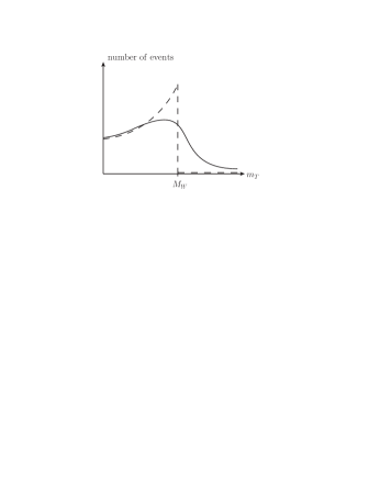
Figure 8: (a) Sketch of the transverse mass distribution for $W$-boson production at hadron colliders, for a perfect detectors and without width effects (dashed), and including detector smearing and width effects (solid).

At lepton colliders, the $W$-mass can be measured from the invariant mass distribution in the processes $e^{+}e^{-}\to W^{+}W^{-}\to qqqq$ and $e^{+}e^{-}\to W^{+}W^{-}\to qq\ell\nu$. The reconstruction of both the transverse and longitudinal components the neutrino momentum is possible here, since there is no ambiguity due to the momentum carried away by the proton remnants.

Alternatively, one may measure $M_{W}$ from a threshold scan, by measuring the cross-section for $e^{+}e^{-}\to W^{+}W^{-}$ at a few center-of-mass energies near $2M_{W}$. Since the cross-section near threshold is small, this approach requires a large amount of luminosity. With the available statistics at LEP, the achievable precision was rather low [54].

For the theoretical description of the cross-section as a function of $\sqrt{s}$ near threshold, one needs to compute the full process $e^{+}e^{-}\to qqqq/qq\ell\nu$, since contributions where the $W$-bosons are off-shell are important for $\sqrt{s}\lesssim 2M_{W}$. In fact, in this regime diagrams without a $W^{+}W^{-}$ pair also contribute significantly. The currently most accurate calculation includes full NLO corrections to the $e^{+}e^{-}\to 4f$ process [55].

The most precise available $M_{W}$ measurements are [54, 56, 57]

$$M_{W}=\; 80.376\pm 0.033\;\text{GeV} (m_{\rm inv}\text{ @ LEP})$$

$$80.387\pm 0.016\;\text{GeV} (m_{\rm T}\text{ @ TeVatron})$$

$$80.370\pm 0.019\;\text{GeV} (m_{\rm T}\text{ @ ATLAS})$$ (99)

3.4 Future $e^{+}e^{-}$ colliders

The experimental precision of EWPOs could be significantly improved at an $e^{+}e^{-}$ collider with much larger luminosity than LEP or SLD. Such machines are proposed primarily for the purpose of detailed measurements of Higgs boson properties, but they could also perform electroweak measurements at $\sqrt{s}\sim M_{Z}$ and $\sqrt{s}\sim 2M_{W}$. The FCC-ee [58] and CEPC [59] concepts are based on circular colliders, where the ILC concept [60, 61] envisions a linear setup. The baseline run scenario for ILC does not include any runs on the $Z$ pole and near the $WW$ threshold, but it can study electroweak physics at a higher energy $\sqrt{s}\sim 250$ GeV by using the radiative return method, where radiation of initial-state photons results in a lower effective center-of-mass energy [see eq. (91)].

The following table illustrates the expected improved precision for a few selected EWPOs:

	today	FCC-ee	CEPC	ILC
$\Gamma_{Z}$ [MeV]	2.3	0.1	0.5	–
$\sin^{2}\theta_{\rm eff}^{\ell}$ [$10^{-5}$]	13	0.5	$<1$	$\sim 2$
$M_{W}$ [MeV]	12	$\lesssim 1$	$\sim 1$	2.4

3.5 Low-Energy EWPOs

Electroweak physics can also be studies with precision experiments performed at lower energies, where the $W$ and $Z$ bosons appear only as virtual particles. An overview of some variety of such experiments can be found in Ref. [62]. In the following, two types of such electroweak precision tests will be briefly described.

Polarized electron scattering:

A beam of left- or right-handed $e^{-}$ is scattered off target particles $X$, where $X$ could be electrons, protons, deuterons, or heavier nuclei. If $X$ is a hadronic or nuclear target, it is advantageous to choose the kinematics such that the momentum transfer is small, $q^{2}\ll m_{p}^{2}$, so that the proton (or nucleus) can be regarded as approximately pointlike.

While the cross-section overall is strongly dominated by t-channel photon exchange, one can probe electroweak physics through the left-right asymmetry

$$A_{\rm LR} =\frac{\sigma_{\rm L}-\sigma_{\rm R}}{\sigma_{\rm L}+\sigma_{\rm R}}$$ (100)

For electron-proton scattering in the limit $$q^{2}\ll m_{p}^{2}$$, this asymmetry is given by, at tree-level,

$$A_{\rm LR}^{ep} \approx\frac{G_{\mu}(-q^{2})}{4\sqrt{2}\pi\alpha}(1-4s_{\scriptscriptstyle{\mathrm{W}}}^{2})$$ (101)

Thus a measurement of $A_{\rm LR}^{ep}$ can be used to determine the weak mixing angle.

Higher-order radiative corrections can be accounted for by replacing the on-shell weak mixing angle $s_{\scriptscriptstyle{\mathrm{W}}}$ with the effective weak mixing angle $\sin^{2}\theta_{\rm eff}$, and by including additional correction factors:

$$1-4s_{\scriptscriptstyle{\mathrm{W}}}^{2}\quad\to\quad 1-4\kappa\sin^{2}\theta_{\rm eff}^{\ell}+\Delta Q$$ (102)

$\kappa$ includes large corrections from the $\gamma$–$Z$ mixing self-energy, which are enhanced by large logarithms:

$$\kappa\approx 1-\frac{c_{\scriptscriptstyle{\mathrm{W}}}}{12\pi^{2}s_{\scriptscriptstyle{\mathrm{W}}}}\sum_{f}v_{f}(eQ_{f})\ln\frac{m_{f}^{2}}{M_{Z}^{2}}$$ (103)

Similar to the logarithms in the charge renormalization, eq. (25), these are ill-defined for light quarks, $f=u,d,s$.

Similar to what is done for $\Delta\alpha$, one may try to extract the hadronic corrections to $\kappa$ from data for $R(s)=\frac{\sigma[e^{+}e^{-}\to\text{hadrons}]}{\sigma[e^{+}e^{-}\to\mu^{+}\mu^{-}]}$ using a dispersion integral. However, this requires additional assumptions in this case, such as SU(3)_u,d,s flavor symmetry [63, 64, 65, 66], because the $Z$ couplings have a different dependence on the fermion flavor that $\gamma$ couplings.

Alternative, the leading hadronic effects can be absorbed into a running $\overline{{\mathrm{MS}}}$ weak mixing angle [67, 12],

$$\kappa\sin^{2}\theta_{\rm eff}^{\ell}\approx\sin^{2}\overline{\theta}(\mu^{2}=-q^{2})\equiv\frac{\overline{g}^{\prime 2}(\mu)}{\overline{g}^{2}(\mu)+\overline{g}^{\prime 2}(\mu)}\bigg{|}_{\mu^{2}=-q^{2}}$$ (104)

where the bar above an expression denotes that this quantity is defined in the $\overline{{\mathrm{MS}}}$ scheme.

The following table lists some of the current and near-future electron-electron and electro-proton scattering experiments, together with their precision in measuring the weak mixing angle [68, 69, 70, 71]:

	$ee$	$ep$
current	E158 (0.5%)	Qweak (0.5%)
future	MOLLER (0.1%)	P2 (0.1%)

The anticipated precision of the future MOLLER and P2 experiments will be comparable to the combined $Z$-pole analysis from LEP/SLC, but in an entirely different setup at low energies, with different sources of experimental and theoretical systematic errors. A more comprehensive exposition of these types of experiments can be found $e.\,g.$ in Ref. [72].

Muon anomalous magnetic moment:

Charged fermions have a magnetic moment with the magnitude $\frac{eQ_{f}}{2m_{f}}g_{f}$, where $g_{f}$ is called the Landé factor. At tree-level ($e.\,g.$ from the Dirac equation) $g_{f}=2$. However, the value of $g_{f}$ gets modified through radiative corrections, generating an anomalous magnetic moment $a_{f}=(g_{f}-2)/2\neq 0$.

In the following we focus on the anomalous magnetic moment of leptons [73, 74]. The main contribution to $a_{\ell}$ stems from QED, which has been computed up to ${\cal O}(\alpha^{5})$, see eq. (59).

Electroweak and hadronic corrections are suppressed by powers of $m_{\ell}^{2}/M_{W}^{2}$ and $m_{\ell}^{2}/\Lambda_{\rm QCD}^{2}$, respectively. Thus they are negligble for the electron magnetic moment, but they become imporant for $\ell=\mu$. The hadronic corrections are relatively large and are typically extracted from data for $R(s)=\frac{\sigma[e^{+}e^{-}\to\text{hadrons}]}{\sigma[e^{+}e^{-}\to\mu^{+}\mu^{-}]}$ [75, 14, 15]. The experimental error of this data is the dominant uncertainty in the theoretical prediction of $a_{\mu}$. Efforts to compute the hadronic corrections using lattice QCD have made a lot of progress recently [76, 77].

The electroweak effects are rather small,

$$a_{\mu}^{\rm EW}=\frac{g^{2}}{16\pi^{2}}\,\frac{m_{\mu}^{2}}{M_{W}^{2}}\times{\cal O}(1)\sim 1.5\times 10^{-9}$$ (105)

but need to be taken into account given the experimental precision for the measurement of $a_{\mu}$. The most precise experimental value is from the g–2 experiment at BNL [78], which yielded

$$a_{\mu}^{\rm exp}=(11\,659\,208.0\pm 6.3)\times 10^{-10}$$ (106)

which differs from the SM prediction [27]

$$a_{\mu}^{\rm exp}=(11\,659\,184.6\pm 4.7)\times 10^{-10}$$ (107)

by more than 3 standard deviations. An ongoing experiment at FNAL aims to improve the precision of $a_{\mu}^{\rm exp}$ by a factor 4 [79].

Exercise:

The electroweak corrections in (105) are proportional to $m_{\mu}^{2}$, and most corrections from BSM physics would have the same proportionality. One power of $m_{\mu}$ stems from the fact that the magnetic moment coupling ${\cal L}\supset\text{const.}\times\overline{\psi}\sigma_{\mu\nu}F^{\mu\nu}\psi$ involves a derivative inside the field strength tensor and thus is proportional to the overall energy scale of the process. Where does the other power of $m_{\mu}$ comes from? Can it be replaced by something else in some new physics model?

4 Tests of the Standard Model and Physics Beyond the Standard Model

4.1 Standard Model predictions

The consistency and accuracy of the SM as a description of electroweak physics can be tested by comparing experimental data for EWPOs with theoretical predictions, where the latter care computed within the SM in as a function of a set of input parameters. All the EWPOs discussed in the previous section can be used for this purpose: $\Gamma_{Z}$, $\sigma_{f}^{0}$, $\sin^{2}\theta_{\rm eff}^{f}$, $M_{W}$ (predicted from $G_{\mu}$), $a_{\mu}$, etc.

Owing to the precision of the available experimental data, higher-order corrections need to be included in this comparison. For all EWPOs listed above, complete two-loop corrections are known, as well as some partial higher-order contributions, in particular from QED and QCD effects (see Refs. [22, 80, 81, 82, 83, 84] and references therein). While the one-loop corrections can be evaluated analytically, with logarithms and dilogathrims appearing in the final result [21], the is in general not the case at the two-loop level and beyond. Instead one needs to result to either approximations or numerical methods. The numerical approaches can be divided into two groups:

• General techniques that can in principle be applied to problems with any number of loops, external legs and types of particles. The best-known approach in this category is sector decomposition [85], which allows one to extract all UV and IR singularities with an algorithm that can be implemented in computer programs and then integrate the coefficients of the singularities and the finite remainder numerically [86, 87, 88, 89]. Another approach, which is not fully general but works for many two- and three-loop applications, is based on Mellin-Barnes representations [90, 91]. The disadvantage of these techniques is their relatively large need of computing resources for the evaluation of multi-dimensional numerical integrals that are slowly converging.

• A range of numerical methods have been tailored for a particular type of problem, $i.\,e.$ self-energy or vertex integrals of a certain loop order. While limited in scope, these approaches tend to produce numerical integrals of lower dimensionality and more favorable convergence behavior than the general techniques. A review of can be found in Ref. [22].

It is instructive to look at some of the leading effects of the radiative corrections. For this purpose, let us consider the corrections to the Fermi constant, see eq. (57), and to the effective weak mixing angle, see eq. (86). They may be written as

$$\frac{G_{\mu}}{\sqrt{2}}=\frac{g^{2}}{8M_{W}^{2}}(1+\Delta r), \Delta r =\Delta\alpha-\frac{c_{\scriptscriptstyle{\mathrm{W}}}^{2}}{s_{\scriptscriptstyle{\mathrm{W}}}^{2}}\Delta\rho+\Delta r_{\rm rem},$$ (108)

$$\sin^{2}\theta_{\rm eff}^{f}=s_{\scriptscriptstyle{\mathrm{W}}}^{2}(1+\Delta\kappa), \Delta\kappa =\frac{c_{\scriptscriptstyle{\mathrm{W}}}^{2}}{s_{\scriptscriptstyle{\mathrm{W}}}^{2}}\Delta\rho+\Delta\kappa_{\rm rem}$$ (109)

Here $\Delta r$ and $\Delta\kappa$ include all higher-order corrections. Two leading contributions can be identified:

The shift in the fine structure constant, $\Delta\alpha$, has already been discussed on page 2.1. It receives numerically comparable contributions from both leptonic and hadronic loops, which add up to

$$\Delta\alpha=\Delta\alpha_{\rm lept}+\Delta\alpha_{\rm had}\approx 6\%$$ (110)

The numerical enhancement stems from the logarithmic dependence on light fermion masses, see eq. (25).

On the other hand, $\Delta\rho$ contains contributions that are proportional to the Yukawa couplings of fermions inside the loop, where the top Yukawa $y_{t}\approx 1$ dominates, whereas all other fermions are negligible:

$$\Delta\rho=\frac{3y_{t}^{2}}{32\pi^{2}}+\underbrace{...}_{\text{fermions other than the top}}\hskip 40.00006pt$$ (111)

It appears in $\Delta r$ and $\Delta\kappa$ in the combination $\frac{c_{\scriptscriptstyle{\mathrm{W}}}^{2}}{s_{\scriptscriptstyle{\mathrm{W}}}^{2}}\Delta\rho\approx 3\%$. The remaining corrections are numerically smaller: $\Delta r_{\rm rem}$, $\Delta\kappa_{\rm rem}\lesssim 1\%$.

When comparing $G_{\mu}$, $M_{W}$ and $\sin^{2}\theta_{\rm eff}^{f}$ to data, the dominant effect of $\Delta\rho$ leads to a relatively precise indirect determination of the top mass, $m_{t}=y_{t}v/\sqrt{2}=176.3\pm 1.9\,$GeV, which agrees reasonably well with the direct measurement from LHC and Tevatron, $m_{t}^{\rm exp}=172.9\pm 0.3\,$GeV (see section 10 of Ref. [27]).

On the other hand, the indirect determination of $M_{H}$ from electroweak precision data is much less accurate [27], since the $M_{H}$ only appears in the small terms $\Delta r_{\rm rem}$, $\Delta\kappa_{\rm rem}$, and the functional dependence on $M_{H}$ is only logarithmic.

The numerically large quadratic dependence on $y_{t}$ in $\Delta\rho$ can be explained through the breaking of custodial symmetry. This is a symmetry of the Higgs potential, which can be most easily seen by re-writing the Higgs field as a matrix. Since the complex Higgs field $\phi=\begin{pmatrix}\phi^{+}\\ \phi^{0}\end{pmatrix}$ has four physical degrees of freedom, one can arrange these four components into a matrix,

$$\Omega=\begin{pmatrix}\phi^{0*}&\phi^{+}\\ \phi^{-}&\phi^{0}\end{pmatrix}$$ (112)

where $\phi^{0*}$ and $\phi^{-}$ are the conjugate fields of $\phi^{0}$ and $\phi^{+}$, respectively. Then the scalar potential becomes

$$V=-\mu^{2}|\phi|^{2}+\lambda|\phi|^{4}=-\frac{\mu^{2}}{2}\,\text{Tr}\{\Omega^{\dagger}\Omega\}+\frac{\lambda}{4}\bigl{(}\text{Tr}\{\Omega^{\dagger}\Omega\}\bigr{)}^{2}$$ (113)

In this form, one can see that $V$ is manifestly invariant under transformations

$$\Omega\to L\Omega R^{\dagger},\qquad L\in\text{SU(2)}_{L},\quad R\in\text{SU(2)}_{R}$$ (114)

where $L,R$ are unitary SU(2) matrices. Since $L$ and $R$ can be independent of each other, they are part of two separate symmetry groups, labeled SU(2)_L,R. SU(2)_L is the usual weak symmetry group.

When $\phi$ obtains a vev, $\langle\Omega\rangle=\begin{pmatrix}v&0\\ 0&v\end{pmatrix}$, the symmetry (114) will be broken, but $\langle\Omega\rangle$ is still invariant under a symmetry sub-group where $L=R\equiv V$:

$$\langle\Omega\rangle\to V\langle\Omega\rangle V^{\dagger},\qquad V\in\text{SU(2)}_{\rm diag}$$ (115)

$\text{SU(2)}_{\rm diag}$ is called the “custodial symmetry” group. The SM Higgs potential, Higgs vev, and weak and QCD gauge interactions are invariant under it, but not the Yukawa couplings. As an example, let us consider the Yukawa couplings of the top and bottom quarks,

$${\cal L}_{\rm Yuk,tb}=-y_{t}\overline{Q}_{3L}\tilde{\phi}\,t_{R}-y_{b}\overline{Q}_{3L}\phi\,b_{R}+\text{h.c.},\qquad\overline{Q}_{3L}=\begin{pmatrix}t_{L}\\ b_{L}\end{pmatrix}$$ (116)

Here $\tilde{\phi}=C\phi^{*}$, and $C=i\sigma^{2}$ is the charge conjugation matrix. If $y_{t}$ and $y_{b}$ were equal, $y_{t}=y_{b}\equiv y$, this could be re-written as

$${\cal L}_{\rm Yuk,tb}=-y\,\overline{Q}_{3L}\Omega\,Q_{3R}+\text{h.c.},\qquad\overline{Q}_{3R}=\begin{pmatrix}t_{R}\\ b_{R}\end{pmatrix}$$ (117)

which would be invariant under $\text{SU(2)}_{\rm diag}$ if the quarks doublets transform as $Q_{L,R}\to VQ_{L,R}$.

However, the fact that $y_{t}\neq y_{b}$ leads to breaking of $\text{SU(2)}_{\rm diag}$. Any breaking effect must be proportional to some power of $(y_{t}-y_{b})^{2}\approx y_{t}^{2}$, so that is vanishes in the limit where $\text{SU(2)}_{\rm diag}$ is restored. This is the origin of the effect in $\Delta\rho$ proportional to $y_{t}^{2}$.

Note that $\text{SU(2)}_{\rm diag}$ is also broken by the hypercharge gauge coupling, but the numerical impact of that in EWPOs is smaller.

4.2 Constraints on Physics Beyond the Standard Model

A global fit to all relevant EWPOs yields good agreement within the SM [27], and there is no obvious hint for BSM physics, except for the discrepancy in the $a_{\mu}$ (see section 3.5). Thus the data can be used to set constraints on new physics models. Based on the discussion from the previous subsection, one can already conclude the models with new sources of custodial symmetry breaking will be severely bounded by electroweak precision data.

If one assumes that the new degree of freedom beyond the SM are heavy compared to the electroweak scale, one BSM effects in EWPOs can be parametrized in a model-independent way by adding higher-dimensional operators to the theory. This framework is often referred to as SMEFT (SM Effective Field Theory). The leading contribution for EWPOs stems from dimension-6 operators,

$${\cal L}={\cal L}_{\rm SM}+\sum_{i}\frac{C_{i}}{\Lambda^{2}}{\cal O}_{i},$$ (118)

where $\Lambda\gg v$ is the mass scale of the BSM physics (typically the smallest BSM mass if there is a more complex particle spectrum). The complete list of dimension-6 operators ${\cal O}_{i}$ can be found $e.\,g.$ in Ref. [92]. The values of the Wilson coefficients depend on the underlying BSM physics, and they can be computed in terms of the parameters of a specific hypothetical model (a procedure called “matching”).

By comparing data to predictions for EWPOs within SMEFT, constraints on the Wilson coefficients of a subset of operators can be derived. The subset that EWPOs are sensitive to includes operators that modify gauge-boson–fermion couplings, Higgs-boson–gauge-boson interactions, and certain four-fermion interactions. In principle, these constraints can be derived in a model-independent fashion, but since there are more operators than independent observables, certain assumptions are typically imposed. For example, one may assume flavor universality, which means that the Wilson coefficients for operators involving fermions are the same for all three fermion generations.

A more detailed description of SMEFT and its applications can be found in the lectures on “Standard Model Effective Field Theories” in this school [93].

In the following, we will instead focus on BSM models where the scale of new physics is lower, $\Lambda\lesssim v$, and thus the SMEFT is not applicable. In the spirit of the school’s theme, “The Obscure Universe: Neutrinos and Other Dark Matters,” the focus is on examples that relate to neutrino and dark matter physics.

4.3 Neutrino Counting

Decays of the $Z$ boson to neutrinos are invisible to collider detectors. However, the existence of this decay channel can be probed by determining the total width $\Gamma_{Z}$ from a fit to the Breit-Wigner lineshape and subtracting the rates for all visible decay channels from it,

$$\Gamma_{Z}=3\,\Gamma_{\ell}+N_{\nu}\Gamma_{\nu}+\Gamma_{\rm had}$$ (119)

Here the masses of charged leptons and neutrinos have been neglected, so that $\Gamma_{e}=\Gamma_{\mu}=\Gamma_{\tau}\equiv\Gamma_{\ell}$ and $\Gamma_{\nu_{e}}=\Gamma_{\nu_{\mu}}=\Gamma_{\nu_{\tau}}\equiv\Gamma_{\nu}$. $N_{\nu}$ is the number of neutrino species ($N_{\nu}=3$ in the SM).

$\Gamma_{\ell}$ and $\Gamma_{\nu}$ are not observables by themselves. However, they can be related to observables as follows [5, 47]:

$$N_{\nu} =\biggl{[}\biggl{(}\frac{12\pi}{M_{Z}^{2}}\,\frac{R_{\ell}}{\sigma^{0}_{\rm had}}\biggr{)}^{2}-R_{\ell}-3\biggr{]}\,\frac{\Gamma_{\ell}}{\Gamma_{\nu}}$$ (120)

Here

$$\sigma^{0}_{\rm had} =\sigma_{e^{+}e^{-}\to\rm had}(s{=}M_{Z}^{2})=\frac{12\pi}{M_{Z}^{2}}\,\frac{\Gamma_{\ell}\Gamma_{\rm had}}{\Gamma_{Z}^{2}},$$ (121)

$$R_{\ell} =\frac{\Gamma_{\rm had}}{\Gamma_{\ell}}=\frac{\sigma^{0}_{\rm had}}{\sigma^{0}_{\ell}}$$ (122)

can be determined from data, and “had” refers to all hadronic final state ($i.\,e.$ summing over all quarks $q\neq t$ in the partonic picture). On the other hand, $\Gamma_{\ell}/\Gamma_{\nu}$ is computed in the SM, but the result is correct also in a variety of models with extended neutrino sectors. Using measurements from LEP, one finds [47]

$$N_{\nu}=2.996\pm 0.007$$ (123)

in agreement with SM expectations.

If one assumes that any BSM neutrino is part of an SU(2)_L doublet together with a new charged lepton ($i.\,e.$ a fourth lepton family), an additional constraint follows from the contribution of this lepton doublet to $\Delta\rho$:

$$\Delta\rho_{\nu\ell 4}=\frac{1}{32\pi^{2}}\biggl{[}\underbrace{y^{2}_{\ell 4}+y^{2}_{\nu 4}-\frac{4y^{2}_{\ell 4}y^{2}_{\nu 4}}{y^{2}_{\ell 4}-y^{2}_{\nu 4}}\ln\frac{y_{\ell 4}}{y_{\nu 4}}}_{\geq(y_{\ell 4}-y_{\nu 4})^{2}}\biggr{]}$$ (124)

Here $y_{\ell 4}$ and $y_{\nu 4}$ are the Yukawa couplings of the extra charged lepton and extra neutrino, respectively. The expression in [ ] can be shown to be bounded from below by $(y_{\ell 4}-y_{\nu 4})^{2}$.

EWPO data puts a constraint on any new physics contributions to $\Delta\rho$, leading to the bound (at 90% confidence level) [27]

$$|y_{\ell 4}-y_{\nu 4}|<48\,\text{GeV}$$ (125)

Extra charged leptons would be visible in particles detectors, of course. Searches at LEP2 exclude the existence of any such particle with mass below 101 GeV [27]. Together with (125) this implies that a 4th generation neutrino with $m_{\nu 4}<50$ GeV is excluded.

At the same time, studies of the $H\to\gamma\gamma$ rate forbid the existence of a 4th lepton family where both the $\ell_{4}$ and $\nu_{4}$ are heavy [94], so that the combination of electroweak precision and Higgs data fully rules out the existence of a sequential 4th fermion generation.

4.4 Sterile Neutrinos

The bounds in the previous subsection do not apply to new neutral fermions that are singlets under SU(2)_L, $i.\,e.$ that do not (electro)weak interactions. Such particles are called sterile neutrinos or right-handed neutrinos, since they can form Yukawa couplings with the SM neutrinos.

Let us consider a model where two such sterile neutrinos are added, denoted $N_{R}^{1}$ and $N_{R}^{2}$, with the interaction Lagrangian [95]

$${\cal L}={\cal L}_{\rm SM}+\sum_{k}i\overline{N}_{R}^{k}\not{\partial}N_{R}^{k}-\Bigl{[}\sum_{\alpha}Y_{\nu\alpha}\overline{L}_{\alpha L}\tilde{\phi}N_{R}^{1}-M\,\overline{N}_{R}^{1}CN_{R}^{2}+\text{h.c.}\Bigr{]}$$ (126)

Here $L_{1L}=\begin{pmatrix}\nu_{eL}\\ e_{L}\end{pmatrix}$ etc. are the SM lepton doublets and $C$ is again the charge conjugation matrix.

In the limit that $M$ is much larger than the observed light neutrino masses, the mass eigenstates of the model are:

• A pseudo-Dirac sterile neutrino $N$ with mass $\approx M$. Here the term “pseudo-Dirac” is used for a pair of Majorana fields with nearly degenerate masses, which behave like a single Dirac particle in some phenomenological contexts. $N$ is mostly composed of $N_{R}^{1,2}$, with a small admixture of left-handed SM neutrinos $\nu_{\alpha L}$, so that is has strongly suppressed couplings to other SM particles and could have escaped detection until now.

• Active Majorana neutrinos $\nu^{\prime}_{e,\mu,\tau}$, which are mostly SM-like, with a small admixture of $N_{R}^{1,2}$, where the mixing angle is approximately given by $\theta_{\alpha}\approx\frac{Y_{\nu\alpha}v}{\sqrt{2}M}$.

Assuming that $M>v$, the main phenomenological effect of this model, compared to the SM, are reduced couplings of the active neutrinos to gauge bosons.

• In muon decay, $\mu\to e\nu^{\prime}_{\mu}\bar{\nu}^{\prime}_{e}$, the relationship between Fermi constant and SM parameters is modifieid according to

  $$\frac{G_{\mu}}{\sqrt{2}}=\frac{g^{2}}{8M_{W}^{2}}(1+\Delta r)(1-\theta_{e}^{2})(1-\theta_{\mu}^{2})$$ (127)

• The invisible $Z$ decay rate is reduced,

  $$\Gamma_{Z\to\rm inv}=\Gamma_{\nu}^{\rm SM}\Bigl{(}N_{\nu}-\sum_{\alpha,\beta}\theta_{\alpha}\theta_{\beta}\Bigr{)}$$ (128)

In the above formulae, $\sin\theta_{\alpha}$ and $\cos\theta_{\alpha}$ have been expanded for $\theta_{\alpha}\ll 1$. Comparing these expressions to electroweak precison data, one obtains the bounds [95]

$$\theta^{2}_{e},\theta^{2}_{\mu} \lesssim 2\times 10^{-3}, \theta^{2}_{\tau} \lesssim 7\times 10^{-3}$$ (today)

$$\lesssim 2\times 10^{-5}, \lesssim 10^{-3}$$ (FCC-ee)

$$\lesssim 2\times 10^{-5}, \lesssim 3\times 10^{-3}$$ (CEPC) (129)

Exercise:

Assuming a special scenario where $\theta_{e}=\theta_{\mu}=\theta_{\tau}\equiv\theta$, what bound on $\theta$ (at 95% C.L.) to you obtain from (128). Use numbers from section 10 in Ref. [27] for $\Gamma_{Z\to\rm inv}^{\rm exp}$ and $\Gamma_{\nu}^{\rm SM}$.

4.5 Dark Photon

Dark photon models are extensions of the SM with an additional U(1) gauge boson, $Z^{\prime}$ that can kinetically mix with the hypercharge gauge boson (see Ref. [96] for a recent review). Let us furthermore introduce a fermion $\chi$ as a dark matter (DM) candidate that couples to $Z^{\prime}$ with coupling strength $g_{D}$. The Lagrangian is given by

$${\cal L}={\cal L}_{\rm SM}-\frac{1}{4}Z^{\prime}_{\mu\nu}Z^{\prime\mu\nu}+\frac{M_{Z^{\prime}}^{2}}{2}Z^{\prime}_{\mu}Z^{\prime\mu}+\overline{\chi}(i\not{\partial}+g_{D}\not{Z}^{\prime}-m_{\chi})\chi+\frac{\epsilon}{2c_{\scriptscriptstyle{\mathrm{W}}}}Z^{\prime}_{\mu\nu}B^{\mu\nu}$$ (130)

Here we have written an explicit mass term for $Z^{\prime}$ for simplicity. In a realistic model this mass would need to be generated through the Higgs or Stückelberg mechanism, but the details are unimportant for the following discussion.

The kinetic terms can be diagonalized can canonically normalized by transforming $Z^{\prime}$ and $B$ to the new fields $Z^{\mu}_{D,0}$ and $B^{\mu}_{0}$ according to

$$\begin{pmatrix}Z^{\mu}_{D,0}\\ B^{\mu}_{0}\end{pmatrix}\approx\begin{pmatrix}1-2\epsilon^{2}/c_{\scriptscriptstyle{\mathrm{W}}}^{2}&0\\ -\epsilon/c_{\scriptscriptstyle{\mathrm{W}}}&1\end{pmatrix}\begin{pmatrix}Z^{\prime\mu}\\ B^{\mu}\end{pmatrix}+{\cal O}(\epsilon^{3})$$ (131)

When expressing ${\cal L}$ in terms of the $Z^{\mu}_{D,0}$ and $B^{\mu}_{0}$, one can see that the dark photon field $Z^{\mu}_{D,0}$ has ${\cal O}(\epsilon)$ couplings to the SM fermions.

After electroweak symmetry breaking, mass mixing between $B_{0}^{\mu}$, $W_{0}^{\mu}$ and $Z^{\mu}_{D,0}$ produces the observable photon and $Z$-boson, as well as the “dark photon” mass eigenstate $Z_{D}$ with mass $M_{Z_{D}}$. Note that the mass mixing between $Z^{\mu}_{D,0}$ and the other fields is also suppressed by $\epsilon$. As a result, the $Z$-boson mass is shifted by an ${\cal O}(\epsilon^{2})$ contribution relative to the SM [97],

$$M_{Z}^{2}\approx\frac{M_{W}^{2}}{c_{\scriptscriptstyle{\mathrm{W}}}^{2}}\Bigl{(}1+\epsilon^{2}\frac{s_{\scriptscriptstyle{\mathrm{W}}}^{2}}{c_{\scriptscriptstyle{\mathrm{W}}}^{2}}\Bigr{)}$$ (132)

where $s_{\scriptscriptstyle{\mathrm{W}}}$ and $c_{\scriptscriptstyle{\mathrm{W}}}$ are the sine and cosine of the weak mixing angle defined through the (tree-level) gauge-couplings, $s_{\scriptscriptstyle{\mathrm{W}}}=g^{\prime}/\sqrt{g^{2}+g^{\prime 2}}$, $c_{\scriptscriptstyle{\mathrm{W}}}=g/\sqrt{g^{2}+g^{\prime 2}}$.

The $Zff$ vector and axial-vector couplings, see eq. (78), are additionally modified through $Z$–$Z_{D}$ mass mixing, leading to [97]

$$v_{f} \approx\frac{e}{2s_{\scriptscriptstyle{\mathrm{W}}}c_{\scriptscriptstyle{\mathrm{W}}}}\biggl{[}\Bigl{(}1-\frac{\alpha^{2}}{2}\Bigr{)}\bigl{(}I_{f}^{3}-2s_{\scriptscriptstyle{\mathrm{W}}}^{2}Q_{f}\bigr{)}+\alpha\epsilon\frac{s_{\scriptscriptstyle{\mathrm{W}}}^{2}}{c_{\scriptscriptstyle{\mathrm{W}}}^{2}}\bigl{(}Q_{f}-I^{3}_{f}\bigr{)}\biggr{]},$$ (133)

$$a_{f} =v_{f}|_{Q_{f}\to 0}$$ (134)

where

$$\alpha =\frac{\epsilon s_{\scriptscriptstyle{\mathrm{W}}}}{c_{\scriptscriptstyle{\mathrm{W}}}(M^{2}_{Z^{\prime}}/M^{2}_{Z,0}-1)}\,,\qquad M_{Z,0}=\frac{M_{W}}{c_{\scriptscriptstyle{\mathrm{W}}}}$$ (135)

As a result, the predictions for all $Z$-pole EWPOs are modified, such as $\Gamma_{Z}$, the $Z$ branching ratios, and $\sin^{2}\theta_{\rm eff}^{f}$.

Additionally, the dark photon also leads to a correction of the electron and muon magnetic moments [98],

$$\delta a_{\ell}=\frac{\alpha\epsilon^{2}}{8\pi}\,F\Bigl{(}\frac{m^{2}_{\ell}}{M^{2}_{Z_{D}}}\Bigr{)}$$ (136)

where $F(x)$ is a function which is $F(x)\approx 1$ for $x\gg 1$ and $F(x)\approx\frac{2}{3}x$ for $x\ll 1$. For some range of $\epsilon$ and $M_{Z_{D}}$, (136) can explain the $>3\sigma$ discrepancy of the muon magnetic moment, see section 3.5. However, for very small values of $M_{Z_{D}}$ the correction to $a_{e}$ also can become sizeable and this region of parameter space is ruled out.

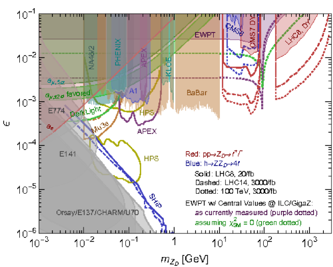
Figure 9: Constraints on the parameter space of the dark photon model (figure taken from Ref. [97]). Electroweak precision constraints from $Z$-pole data are labeled “EWPT” (shaded region for existing constraints and short-dashed lines for future constraints obtainable at ILC). “$a_{\mu,\pm 2\sigma}$ favored” indicates the region that would alleviate the muon magnetic moment discrepancy within 95% confidence level, while the region “$a_{\mu,5\sigma}$” is excluded because it would worsen the discrepancy to the level of 5 standard deviations. The shaded region labeled “$a_{e}$” is excluded from electron magnetic moment constraints. The other shaded regions are excluded by direct searches for $Z_{D}$.

The constraints from $Z$-pole EWPOs and magnetic moments are depicted in Fig. 9, together with bounds from direct searches for $Z_{D}$ at various experiments. Note, however, that the direct search limits assume that $Z_{D}$ only decays into SM particles. These bounds can be relaxed when the invisible decay channel into DM particles, $Z_{D}\to\chi\bar{\chi}$ is kinematically open ($m_{\chi}<M_{Z_{D}}/2$), whereas the bounds from electroweak precision data are independent from such assumptions.

Appendix A Answers to Exercise Questions

Page 2.1:

$$\Sigma_{T}(k^{2})=\frac{\alpha}{3\pi}\biggl{[}\frac{3(d/2-1)k^{2}+6m^{2}}{d-1}B_{0}(k^{2},m^{2},m^{2})-\frac{4(d-2)}{d-1}A_{0}(m^{2})\biggr{]}$$

$$\frac{\partial^{2}}{\partial k_{\mu}\partial k^{\mu}}f(k^{2})=\frac{\partial}{\partial k_{\mu}}\biggl{(}\frac{\partial f}{\partial(k^{2})}\underbrace{\frac{\partial(k^{2})}{\partial k^{\mu}}}_{2k_{\mu}}\biggr{)}=\frac{\partial f}{\partial(k^{2})}2d+\frac{\partial^{2}f}{\partial(k^{2})^{2}}\underbrace{(2k_{\mu})(2k^{\mu})}_{0\text{ for }k^{2}=0}$$

$$\begin{aligned} \frac{\partial}{\partial(k^{2})}&B_{0}(k^{2},m^{2},m^{2})\Big{|}_{k^{2}=0}\\ &=\frac{1}{2d}\,\frac{\partial^{2}}{\partial k_{\mu}\partial k^{\mu}}\biggl{[}\int\frac{d^{d}q\;\omega_{d}}{[q^{2}-m^{2}][(q+k)^{2}-m^{2}]}\biggr{]}_{k^{2}=0}\hskip 70.0001pt\biggl{(}\omega_{d}=\frac{(2\pi\mu)^{4-d}}{i\pi^{2}}\biggr{)}\\ &=\frac{1}{2d}\,\frac{\partial}{\partial k_{\mu}}\biggl{[}\int\frac{d^{d}q\;\omega_{d}\;(-2)(q_{\mu}+k_{\mu})}{[q^{2}-m^{2}][(q+k)^{2}-m^{2}]^{2}}\biggr{]}_{k^{2}=0}\\ &=\frac{1}{2d}\biggl{[}-\int\frac{d^{d}q\;\omega_{d}\;2d}{[q^{2}-m^{2}][(q+k)^{2}-m^{2}]^{2}}+\int\frac{d^{d}q\;\omega_{d}\;8(q+k)^{2}}{[q^{2}-m^{2}][(q+k)^{2}-m^{2}]^{3}}\biggr{]}_{k^{2}=0}\\ &=\frac{1}{2d}\biggl{[}(8-2d)\int\frac{d^{d}q\;\omega_{d}}{[q^{2}-m^{2}]^{3}}+8m^{2}\int\frac{d^{d}q\;\omega_{d}}{[q^{2}-m^{2}]^{4}}\biggr{]}\\ &=\frac{1}{2d}\bigl{[}(8-2d)\tfrac{1}{2}A^{\prime\prime}_{0}(m^{2})+8m^{2}\tfrac{1}{6}A^{\prime\prime\prime}_{0}(m^{2})\bigr{]}\end{aligned}$$

$$\Rightarrow\quad \Sigma^{\prime}_{T}(0)=\frac{\alpha}{3\pi}\biggl{[}\frac{3(d/2-1)}{d-1}\underbrace{B_{0}(0,m^{2},m^{2})}_{A^{\prime}_{0}(m^{2})}+\frac{6m^{2}}{(d-1)2d}\bigl{[}(4-d)A^{\prime\prime}_{0}(m^{2})+\tfrac{4}{3}m^{2}A^{\prime\prime\prime}_{0}(m^{2})\bigr{]}\biggr{]}$$

$$A^{\prime}_{0}(m^{2})=\frac{2}{4-d}-\gamma_{E}-\ln\frac{m^{2}}{4\pi\mu^{2}},\qquad A^{\prime\prime}_{0}(m^{2})=-\frac{1}{m^{2}},\qquad A^{\prime\prime\prime}_{0}(m^{2})=\frac{1}{m^{4}}$$

$$\Rightarrow\quad \Sigma^{\prime}_{T}(0)=\frac{\alpha}{3\pi}\biggl{[}\frac{2}{4-d}-\gamma_{E}-\ln\frac{m^{2}}{4\pi\mu^{2}}+{\cal O}(d-4)\biggr{]}$$

Page 2.2:

$$\delta V=[\text{terms in }\eqref{delV}] +\frac{M_{H}^{2}}{2v}\Bigl{(}\frac{\delta v}{v}+\frac{\delta M_{H}^{2}}{M_{H}^{2}}\Bigr{)}\,h(h^{2}+G_{0}^{2}+2G^{+}G^{-})$$

$$+\frac{M_{H}^{2}}{8v^{2}}\Bigl{(}\frac{\delta v}{v}+\frac{\delta M_{H}^{2}}{M_{H}^{2}}\Bigr{)}\,(h^{2}+G_{0}^{2}+2G^{+}G^{-})^{2}$$

Page 3.1:

• $\alpha$: protected by electromagnetic gauge symmetry;

• $G_{\mu}$: new physics decouples in effective Fermi model (as long as $m_{BSM}\gg m_{\mu}$);

• $\alpha_{\rm s}$: protected by QCD gauge symmetry (lattice), soft-collinear effective theory (event shapes, $\tau$ decays), or not at all (EWPOs);

• $m_{t}$: measurement based on kinematical feature (threshold);

• $M_{Z}$: measurement based on kinematical feature (resonance).

Page 3.5: The magnetic moment interaction flips the chirality of the fermion ($e.\,g.$ left- to right-handed). The only parameters in the SM that break conservation of chirality are the Yukawa couplings (or, equivalently, the fermion masses), and thus any chirality flip must be proportional to $m_{f}$. A new physics model that has an additional source of chirality breaking could change this behavior. For example, if one introduces a second Higgs doublet that does not obtain any vev (and thus does not contribute to the muon mass) but has a Yukawa couplings $Y^{\prime}_{\mu}$ with the muon, it could generate a correction to $a_{\mu}$ proportional to $m_{\mu}Y^{\prime}_{\mu}$ instead of $m_{\mu}^{2}$. Since there are few other bounds on the value of $Y^{\prime}_{\mu}$, this corrections could be relatively large (even though a two-loop diagram would be required).

Page 4.4: According to Tab. 10.6 in [27], $\Gamma_{Z\to\rm inv}^{\rm exp}=498.9\pm 2.5$ MeV and $3\Gamma_{\nu}^{\rm SM}=501.464$ MeV. The uncertainty in the latter is negligible. Using $\Gamma_{Z\to\rm inv}^{\rm exp}=3\Gamma_{\nu}^{\rm SM}(1-3\theta^{2})$ and assuming Gaussian error distribution, we then obtain $\theta^{2}<5\times 10^{-3}$ at 95% C.L.

References

- [1] S. Glashow, Partial Symmetries of Weak Interactions, Nucl. Phys. 22 (1961) 579.
- [2] S. Weinberg, A Model of Leptons, Phys. Rev. Lett. 19 (1967) 1264.
- [3] A. Salam, Weak and Electromagnetic Interactions, Conf. Proc. C 680519 (1968) 367.
- [4] G. ’t Hooft and M. Veltman, Regularization and Renormalization of Gauge Fields, Nucl. Phys. B 44 (1972) 189.
- [5] ALEPH, DELPHI, L3, OPAL, SLD, LEP Electroweak Working Group, SLD Electroweak Group, SLD Heavy Flavour Group collaboration, Precision electroweak measurements on the resonance, Phys. Rept. 427 (2006) 257 [hep-ex/0509008].
- [6] S. Novaes, Standard model: An Introduction, in 10th Jorge Andre Swieca Summer School: Particle and Fields, pp. 5–102, 1, 1999 [hep-ph/0001283].
- [7] M.E. Peskin, Lectures on the Theory of the Weak Interaction, in 2016 European School of High-Energy Physics, pp. 1–70, 2017, DOI [1708.09043].
- [8] A. Arbuzov, Quantum Field Theory and the Electroweak Standard Model, in Proceedings, 2015 European School of High-Energy Physics, M. Mulders and G. Zanderighi, eds., pp. 1–34, 2017, DOI [1801.05670].
- [9] M. Steinhauser, Leptonic contribution to the effective electromagnetic coupling constant up to three loops, Phys. Lett. B 429 (1998) 158 [hep-ph/9803313].
- [10] C. Sturm, Leptonic contributions to the effective electromagnetic coupling at four-loop order in QED, Nucl. Phys. B 874 (2013) 698 [1305.0581].
- [11] J. Erler, Calculation of the QED coupling alpha (M(Z)) in the modified minimal subtraction scheme, Phys. Rev. D 59 (1999) 054008 [hep-ph/9803453].
- [12] J. Erler and R. Ferro-Hernández, Weak Mixing Angle in the Thomson Limit, JHEP 03 (2018) 196 [1712.09146].
- [13] A. Blondel et al., Theory report on the 11th FCC-ee workshop, 1905.05078.
- [14] M. Davier, A. Hoecker, B. Malaescu and Z. Zhang, A new evaluation of the hadronic vacuum polarisation contributions to the muon anomalous magnetic moment and to , Eur. Phys. J. C 80 (2020) 241 [1908.00921].
- [15] A. Keshavarzi, D. Nomura and T. Teubner, of charged leptons, , and the hyperfine splitting of muonium, Phys. Rev. D 101 (2020) 014029 [1911.00367].
- [16] F. Burger, K. Jansen, M. Petschlies and G. Pientka, Leading hadronic contributions to the running of the electroweak coupling constants from lattice QCD, JHEP 11 (2015) 215 [1505.03283].
- [17] M. Cè, T.S. José, A. Gérardin, H.B. Meyer, K. Miura, K. Ottnad et al., The hadronic contribution to the running of the electromagnetic coupling and the electroweak mixing angle, PoS LATTICE2019 (2019) 010 [1910.09525].
- [18] OPAL collaboration, Measurement of the running of the QED coupling in small-angle Bhabha scattering at LEP, Eur. Phys. J. C 45 (2006) 1 [hep-ex/0505072].
- [19] L3 collaboration, Measurement of the running of the electromagnetic coupling at large momentum-transfer at LEP, Phys. Lett. B 623 (2005) 26 [hep-ex/0507078].
- [20] KLOE-2 collaboration, Measurement of the running of the fine structure constant below 1 GeV with the KLOE Detector, Phys. Lett. B 767 (2017) 485 [1609.06631].
- [21] A. Denner, Techniques for calculation of electroweak radiative corrections at the one loop level and results for W physics at LEP-200, Fortsch. Phys. 41 (1993) 307 [0709.1075].
- [22] A. Freitas, Numerical multi-loop integrals and applications, Prog. Part. Nucl. Phys. 90 (2016) 201 [1604.00406].
- [23] S. Willenbrock and G. Valencia, On the definition of the Z boson mass, Phys. Lett. B 259 (1991) 373.
- [24] A. Sirlin, Theoretical considerations concerning the Z0 mass, Phys. Rev. Lett. 67 (1991) 2127.
- [25] R.G. Stuart, Gauge invariance, analyticity and physical observables at the Z0 resonance, Phys. Lett. B 262 (1991) 113.
- [26] P. Gambino and P.A. Grassi, The Nielsen identities of the SM and the definition of mass, Phys. Rev. D 62 (2000) 076002 [hep-ph/9907254].
- [27] Particle Data Group collaboration, Review of Particle Physics, PTEP 2020 (2020) 083C01.
- [28] T. Aoyama, T. Kinoshita and M. Nio, Theory of the Anomalous Magnetic Moment of the Electron, Atoms 7 (2019) 28.
- [29] T. Aoyama, M. Hayakawa, T. Kinoshita and M. Nio, Complete Tenth-Order QED Contribution to the Muon g-2, Phys. Rev. Lett. 109 (2012) 111808 [1205.5370].
- [30] T. Aoyama, M. Hayakawa, T. Kinoshita and M. Nio, Quantum electrodynamics calculation of lepton anomalous magnetic moments: Numerical approach to the perturbation theory of QED, PTEP 2012 (2012) 01A107.
- [31] P. Baikov, A. Maier and P. Marquard, The QED vacuum polarization function at four loops and the anomalous magnetic moment at five loops, Nucl. Phys. B 877 (2013) 647 [1307.6105].
- [32] D. Hanneke, S. Fogwell and G. Gabrielse, New Measurement of the Electron Magnetic Moment and the Fine Structure Constant, Phys. Rev. Lett. 100 (2008) 120801 [0801.1134].
- [33] P.J. Mohr, D.B. Newell and B.N. Taylor, CODATA Recommended Values of the Fundamental Physical Constants: 2014, Rev. Mod. Phys. 88 (2016) 035009 [1507.07956].
- [34] T. Aoyama, T. Kinoshita and M. Nio, Revised and Improved Value of the QED Tenth-Order Electron Anomalous Magnetic Moment, Phys. Rev. D 97 (2018) 036001 [1712.06060].
- [35] R.H. Parker, C. Yu, W. Zhong, B. Estey and H. Muller, Measurement of the fine-structure constant as a test of the Standard Model, Science 360 (2018) 191 [1812.04130].
- [36] T. van Ritbergen and R.G. Stuart, On the precise determination of the Fermi coupling constant from the muon lifetime, Nucl. Phys. B 564 (2000) 343 [hep-ph/9904240].
- [37] M. Steinhauser and T. Seidensticker, Second order corrections to the muon lifetime and the semileptonic B decay, Phys. Lett. B 467 (1999) 271 [hep-ph/9909436].
- [38] A. Pak and A. Czarnecki, Mass effects in muon and semileptonic b —> c decays, Phys. Rev. Lett. 100 (2008) 241807 [0803.0960].
- [39] MuLan collaboration, Measurement of the Positive Muon Lifetime and Determination of the Fermi Constant to Part-per-Million Precision, Phys. Rev. Lett. 106 (2011) 041803 [1010.0991].
- [40] ALPHA collaboration, QCD Coupling from a Nonperturbative Determination of the Three-Flavor Parameter, Phys. Rev. Lett. 119 (2017) 102001 [1706.03821].
- [41] S. Zafeiropoulos, P. Boucaud, F. De Soto, J. Rodríguez-Quintero and J. Segovia, Strong Running Coupling from the Gauge Sector of Domain Wall Lattice QCD with Physical Quark Masses, Phys. Rev. Lett. 122 (2019) 162002 [1902.08148].
- [42] A.H. Hoang, S. Plätzer and D. Samitz, On the Cutoff Dependence of the Quark Mass Parameter in Angular Ordered Parton Showers, JHEP 10 (2018) 200 [1807.06617].
- [43] M. Beneke, P. Marquard, P. Nason and M. Steinhauser, On the ultimate uncertainty of the top quark pole mass, Phys. Lett. B 775 (2017) 63 [1605.03609].
- [44] F. Simon, Scanning Strategies at the Top Threshold at ILC, in International Workshop on Future Linear Colliders, 2, 2019 [1902.07246].
- [45] M. Beneke, Y. Kiyo, P. Marquard, A. Penin, J. Piclum and M. Steinhauser, Next-to-Next-to-Next-to-Leading Order QCD Prediction for the Top Antitop -Wave Pair Production Cross Section Near Threshold in Annihilation, Phys. Rev. Lett. 115 (2015) 192001 [1506.06864].
- [46] M. Beneke, Y. Kiyo, A. Maier and J. Piclum, Near-threshold production of heavy quarks with QQbar_threshold, Comput. Phys. Commun. 209 (2016) 96 [1605.03010].
- [47] P. Janot and S. Jadach, Improved Bhabha cross section at LEP and the number of light neutrino species, Phys. Lett. B 803 (2020) 135319 [1912.02067].
- [48] D. Bardin, A. Leike, T. Riemann and M. Sachwitz, Energy Dependent Width Effects in e+ e- Annihilation Near the Z Boson Pole, Phys. Lett. B 206 (1988) 539.
- [49] J. Ablinger, J. Blümlein, A. De Freitas and K. Schönwald, Subleading Logarithmic QED Initial State Corrections to to , Nucl. Phys. B 955 (2020) 115045 [2004.04287].
- [50] C. Duhr, F. Dulat and B. Mistlberger, The Drell-Yan cross section to third order in the strong coupling constant, 2001.07717.
- [51] CDF, DØ collaboration, Tevatron Run II combination of the effective leptonic electroweak mixing angle, Phys. Rev. D 97 (2018) 112007 [1801.06283].
- [52] ATLAS collaboration, Measurement of the effective leptonic weak mixing angle using electron and muon pairs from -boson decay in the ATLAS experiment at TeV, Tech. Rep. ATLAS-CONF-2018-037, CERN, Geneva (Jul, 2018).
- [53] J. Smith, W. van Neerven and J. Vermaseren, The Transverse Mass and Width of the Boson, Phys. Rev. Lett. 50 (1983) 1738.
- [54] ALEPH, DELPHI, L3, OPAL, LEP Electroweak collaboration, Electroweak Measurements in Electron-Positron Collisions at W-Boson-Pair Energies at LEP, Phys. Rept. 532 (2013) 119 [1302.3415].
- [55] A. Denner, S. Dittmaier, M. Roth and L. Wieders, Electroweak corrections to charged-current e+ e- — 4 fermion processes: Technical details and further results, Nucl. Phys. B 724 (2005) 247 [hep-ph/0505042].
- [56] CDF, DØ collaboration, Combination of CDF and D0 -Boson Mass Measurements, Phys. Rev. D 88 (2013) 052018 [1307.7627].
- [57] ATLAS collaboration, Measurement of the -boson mass in pp collisions at TeV with the ATLAS detector, Eur. Phys. J. C 78 (2018) 110 [1701.07240].
- [58] FCC collaboration, FCC-ee: The Lepton Collider: Future Circular Collider Conceptual Design Report Volume 2, Eur. Phys. J. ST 228 (2019) 261.
- [59] CEPC Study Group collaboration, CEPC Conceptual Design Report: Volume 2 - Physics \& Detector, 1811.10545.
- [60] H. Baer et al., eds., The International Linear Collider Technical Design Report - Volume 2: Physics, 1306.6352.
- [61] P. Bambade et al., The International Linear Collider: A Global Project, 1903.01629.
- [62] J. Erler and S. Su, The Weak Neutral Current, Prog. Part. Nucl. Phys. 71 (2013) 119 [1303.5522].
- [63] W. Wetzel, The Hadronic Contribution to the and Mass, Z. Phys. C 11 (1981) 117.
- [64] W.J. Marciano and A. Sirlin, Testing the Standard Model by Precise Determinations of W+- and Z Masses, Phys. Rev. D 29 (1984) 945.
- [65] F. Jegerlehner, Hadronic Contributions to Electroweak Parameter Shifts: A Detailed Analysis, Z. Phys. C 32 (1986) 195.
- [66] F. Jegerlehner, Variations on Photon Vacuum Polarization, EPJ Web Conf. 218 (2019) 01003 [1711.06089].
- [67] J. Erler and M.J. Ramsey-Musolf, The Weak mixing angle at low energies, Phys. Rev. D 72 (2005) 073003 [hep-ph/0409169].
- [68] SLAC E158 collaboration, Precision measurement of the weak mixing angle in Moller scattering, Phys. Rev. Lett. 95 (2005) 081601 [hep-ex/0504049].
- [69] Qweak collaboration, Precision measurement of the weak charge of the proton, Nature 557 (2018) 207 [1905.08283].
- [70] MOLLER collaboration, The MOLLER Experiment: An Ultra-Precise Measurement of the Weak Mixing Angle Using M{\o}ller Scattering, 1411.4088.
- [71] D. Becker et al., The P2 experiment, 1802.04759.
- [72] K. Kumar, S. Mantry, W. Marciano and P. Souder, Low Energy Measurements of the Weak Mixing Angle, Ann. Rev. Nucl. Part. Sci. 63 (2013) 237 [1302.6263].
- [73] F. Jegerlehner and A. Nyffeler, The Muon g-2, Phys. Rept. 477 (2009) 1 [0902.3360].
- [74] F. Jegerlehner, The Muon g-2 in Progress, Acta Phys. Polon. B 49 (2018) 1157 [1804.07409].
- [75] F. Jegerlehner, Muon g – 2 theory: The hadronic part, EPJ Web Conf. 166 (2018) 00022 [1705.00263].
- [76] H.B. Meyer and H. Wittig, Lattice QCD and the anomalous magnetic moment of the muon, Prog. Part. Nucl. Phys. 104 (2019) 46 [1807.09370].
- [77] S. Borsanyi et al., Leading-order hadronic vacuum polarization contribution to the muon magnetic momentfrom lattice QCD, 2002.12347.
- [78] Muon g-2 collaboration, Measurement of the negative muon anomalous magnetic moment to 0.7 ppm, Phys. Rev. Lett. 92 (2004) 161802 [hep-ex/0401008].
- [79] Muon g-2 collaboration, Muon (g-2) Technical Design Report, 1501.06858.
- [80] I. Dubovyk, A. Freitas, J. Gluza, T. Riemann and J. Usovitsch, Complete electroweak two-loop corrections to Z boson production and decay, Phys. Lett. B 783 (2018) 86 [1804.10236].
- [81] I. Dubovyk, A. Freitas, J. Gluza, T. Riemann and J. Usovitsch, Electroweak pseudo-observables and Z-boson form factors at two-loop accuracy, JHEP 08 (2019) 113 [1906.08815].
- [82] M. Awramik, M. Czakon, A. Freitas and G. Weiglein, Precise prediction for the W boson mass in the standard model, Phys. Rev. D 69 (2004) 053006 [hep-ph/0311148].
- [83] C. Gnendiger, D. Stöckinger and H. Stöckinger-Kim, The electroweak contributions to after the Higgs boson mass measurement, Phys. Rev. D 88 (2013) 053005 [1306.5546].
- [84] A. Czarnecki, W.J. Marciano and A. Vainshtein, Refinements in electroweak contributions to the muon anomalous magnetic moment, Phys. Rev. D 67 (2003) 073006 [hep-ph/0212229].
- [85] T. Binoth and G. Heinrich, An automatized algorithm to compute infrared divergent multiloop integrals, Nucl. Phys. B 585 (2000) 741 [hep-ph/0004013].
- [86] C. Bogner and S. Weinzierl, Resolution of singularities for multi-loop integrals, Comput. Phys. Commun. 178 (2008) 596 [0709.4092].
- [87] S. Borowka, G. Heinrich, S. Jones, M. Kerner, J. Schlenk and T. Zirke, SecDec-3.0: numerical evaluation of multi-scale integrals beyond one loop, Comput. Phys. Commun. 196 (2015) 470 [1502.06595].
- [88] S. Borowka, G. Heinrich, S. Jahn, S. Jones, M. Kerner, J. Schlenk et al., pySecDec: a toolbox for the numerical evaluation of multi-scale integrals, Comput. Phys. Commun. 222 (2018) 313 [1703.09692].
- [89] A.V. Smirnov, FIESTA4: Optimized Feynman integral calculations with GPU support, Comput. Phys. Commun. 204 (2016) 189 [1511.03614].
- [90] M. Czakon, Automatized analytic continuation of Mellin-Barnes integrals, Comput. Phys. Commun. 175 (2006) 559 [hep-ph/0511200].
- [91] I. Dubovyk, J. Gluza, T. Riemann and J. Usovitsch, Numerical integration of massive two-loop Mellin-Barnes integrals in Minkowskian regions, PoS LL2016 (2016) 034 [1607.07538].
- [92] B. Grzadkowski, M. Iskrzynski, M. Misiak and J. Rosiek, Dimension-Six Terms in the Standard Model Lagrangian, JHEP 10 (2010) 085 [1008.4884].
- [93] A. Martin, Standard Model Effective Field Theories, in TASI 2020 "The Obscure Universe: Neutrinos and Other Dark Matters, PoS TASI2020, to appear.
- [94] A. Lenz, Constraints on a fourth generation of fermions from Higgs Boson searches, Adv. High Energy Phys. 2013 (2013) 910275.
- [95] S. Antusch and O. Fischer, Testing sterile neutrino extensions of the Standard Model at future lepton colliders, JHEP 05 (2015) 053 [1502.05915].
- [96] M. Fabbrichesi, E. Gabrielli and G. Lanfranchi, The Dark Photon, 2005.01515.
- [97] D. Curtin, R. Essig, S. Gori and J. Shelton, Illuminating Dark Photons with High-Energy Colliders, JHEP 02 (2015) 157 [1412.0018].
- [98] M. Pospelov, Secluded U(1) below the weak scale, Phys. Rev. D 80 (2009) 095002 [0811.1030].