Shadow surface states in topological Kondo insulators

Abstract

The surface states of 3D topological insulators in general have negligible quantum oscillations when the chemical potential is tuned to the Dirac points. In contrast, we find that topological Kondo insulators can support surface states with an arbitrarily large Fermi surface when the chemical potential is pinned to the Dirac point. We illustrate that these Fermi surfaces give rise to finite-frequency quantum oscillations, which can become comparable to the extremal area of the unhybridized bulk bands. We show that this occurs when the crystal symmetry is lowered from cubic to tetragonal in a minimal two-orbital model. We label such surface modes as ‘shadow surface states’. Moreover, we show that the sufficient NNN out-of-plane hybridization leading to shadow surface states can be self-consistently stabilized for tetragonal topological Kondo insulators. Consequently, shadow surface states provide an important example of high-frequency quantum oscillations beyond the context of cubic topological Kondo insulators.

I Introduction

Kondo insulators are strongly correlated systems where the hybridization between the quasi-localized $f$-electrons and the itinerant conduction electrons leads to an insulating gap at low temperaturesFisk et al. (1995). The archetypal Kondo insulator SmB₆, discovered over 50 years agoMenth et al. (1969), drew revived interest with proposals advancing topological surface states as an explanation for the previously-reported low- temperature resistivity plateauDzero et al. (2010, 2012); Alexandrov et al. (2013); Dzero et al. (2016a). While angle-resolved photoemmission spectroscopy (ARPES) experiments have since resolved these topological surface statesJiang et al. (2013); Kim et al. (2014); Neupane et al. (2013); Frantzeskakis et al. (2013); Denlinger et al. (2014); Xu et al. (2016) a number of puzzles remain, most notably in the linear specific heat with a large Sommerfeld coefficientPhelan et al. (2014), gapless optical conductivityLaurita et al. (2016) and unconventional quantum oscillationsLi et al. (2014); Tan et al. (2015); Hartstein et al. (2018, 2020) (QO’s). Although specific heat and optical conductivity anomalies most likely originate from the bulk of SmB₆, the nature of the QO’s is still under debate. Similar unconventional QO’s have also been observed in another Kondo insulator YbB₁₂Liu et al. (2018); Xiang et al. (2018), suggesting a unified underlying mechanism. Several theoretical proposals based on magnetic breakdownKnolle and Cooper (2015); Zhang et al. (2016), excitonsKnolle and Cooper (2017), impurity statesShen and Fu (2018); Skinner (2019), contribution from Fermi sea Pal (2017), interplay between correlations and nonlocal hybridization Peters et al. (2019), oscillations of the Kondo screening Lu et al. (2020), fractionalizationBaskaran (2015); Erten et al. (2017); Chowdhury et al. (2018); Varma (2020) and surface driven mechanismsAlexandrov et al. (2015); Erten et al. (2016) have been advanced in this context.

A key aspect of QO experiments in SmB₆ is the observation of high-frequency oscillations which apparently match the extremal area of the unhybridized bulk bands. This naturally suggests that the bulk Landau-quantized states underpin the observed oscillations. However, ARPES experimentsJiang et al. (2013); Kim et al. (2014); Neupane et al. (2013); Frantzeskakis et al. (2013); Denlinger et al. (2014); Xu et al. (2016) on SmB₆ indicate a surface-state Fermi surface (FS) with total area which is comparable to the extremal area of the unhybridized bands, which raises the possibility that high QO frequencies are instead rooted in the surface states. Surface Kondo breakdownAlexandrov et al. (2015); Erten et al. (2016) has been proposed as one possible mechanism for the emergence of a ‘large’ FS for the surface states: the Kondo effect is suppressed on the surface, liberating the conduction electrons which contribute directly to the FS of the surface states which expands as a consequence.

Motivated by the well-studied case of SmB₆, we consider the possibility of high-frequency QO in a broader class of topological Kondo insulators (TKIs). In this context, we note that the areas of the surface states are not directly related with the topological nature and but depend in general on the bulk model parameters Roy et al. (2014). Starting from a minimal two-orbital model for cubic TKIs with nearest-neighbor (NN) hybridization, we analyze the effects of tetragonal anisotropy and next-nearest neighbor (NNN) hybridization on the surface-state spectrum. Remarkably, we find that the surface-states have two FS’s at charge neutrality in the extreme limit of vanishing NNN in-plane hybridization. Due to the Kondo effect, which hybridizes quasi-localized and conduction electrons, the two bands have very different effective masses, while having equal FS areas. We refer to these modes as ’shadow surface states.’ The emergence of these shadow states stands in stark contrast to the the surface states of a minimal cubic model at charge neutrality, since the presence of Dirac points in that case effectively excludes any QO due to the surface states. Moreover, the areas enclosed by either of the two FS can be made comparable to the unhybridized area of the bulk FS. In some respect surface states are insensitive to the bulk gap and are holographic projections of bulk unhybridized bands, hence justifying the name of ‘shadow surface states’. Because of the disparity in the effective masses of the ’heavy’ hole-like and ’light’ electron-like bands, the added contributions of the two FS in the presence of a magnetic field can give rise to high-frequency QO. For a finite NNN in-plane hybridization, the two FS’s become gapped and are replaced by a set of Dirac points, with a gap controlled by the relative amplitude of in-plane and out-of plane NNN hybridization. As we discuss in greater detail below, high-frequency QO are still possible in this case.

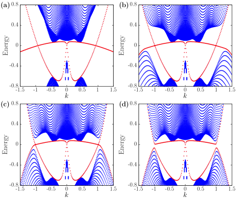
Figure 1: Evolution of the spectrum of a two-orbital model for topological Kondo insulators in the presence of NN and NNN hybridization terms with tetragonal symmetry. The panels correspond to solutions with increasing NNN in-plane hybridization, as determined by the parameter $\beta$ in (3). Blue and red points denote bulk and surface states, respectively. The momentum $k$ is chosen along the $\Gamma$ to $M$ direction ($\theta_{k}=\pi/4$). Panel (a) $(\beta=0)$ illustrates the emergence of shadow states. The second crossing of the two surface bands also occurs for finite momenta along an arbitrary in-plane axis, signaling the presence of a finite FS. Panels (b-d), corresponding to $\beta=0.2,0.3$ and $0.35$ respectively, illustrate the presence and gapping of Dirac points. The associated Lifshitz transitions are discussed in the text. The numerical solutions were obtained for a slab geometry using a lattice model corresponding to $H_{T}$ in (1) with open boundary conditions and 200 lattice sites along the $z$ direction. The parameters of the model are $M^{\prime}=m^{\prime}=-0.45$, $M=m=-0.55$, $v=1.0$ and $\alpha=-6.0$.

In most two-orbital models of non-interacting topological insulators (TIs), the bulk band structure and gap are determined by the direct hybridization between electrons in different orbitals. By contrast, in a minimal two-orbital model for TKIsAlexandrov et al. (2015), the effective hybridization between the orbitals, which leads to a finite gap, can be traced to the Kondo screening, at mean-field level. Consequently, the gap structure and the surface states in TKIs are not determined simply by the overlap of the weakly-interacting orbitals, but rather emerge as a consequence of Kondo interactions, and thus can exhibit a wider array of possible structures.

The TKI mean field model, with additional NNN coupling, retains a strong topological insulator classification upon lowering the point-group symmetry from cubic to tetragonal, as indicated by the changes in the surface-state spectrum. For general NNN hybridization anisotropy, an even number of additional Dirac points appear in the surface-state spectrum. When shadow states with a finite FS emerge, the chemical potential intersects the surface-state bands at an odd number of points along any axis extending from the center of the BZ, as shown in Fig. (1) (a) along $\Gamma$-M.

We further show that the relative strength of NNN and NN hybridization controls the size of the shadow state FS, which approaches the extremal area of the unhybridized bands for specific value of parameters. Although a finite gap opens along the surface-state FS for any finite in-plane NNN hybridization, as previously discussed, we expect it’s effect on the QO is negligible as long as the Landau level spacing is larger than the surface gap. Similar finite gap can also be opened through sharp disorder which initiates large momentum scattering. For sufficiently clean systems their effect on QO should still be minor. Therefore, while the realized shadow states are not symmetry protected, for specific range of NN and NNN hybridizations the QO response due to the shadow states is robust.

Shadow surface states emerge in a natural generalization of a minimal model for cubic TKIs which accounts for tetragonal anisotropy and NNN hybridization. While shadow surface states are not directly relevant to cubic TKIs such as SmB₆ and YbB₁₂, they provide a striking example of surface states which can support high-frequency QO, even near the charge neutrality point in TKIs with tetragonal symmetry. In addition modification of the cubic symmetry of natural materials which accrue on the edge of the system can potentially reduce the symmetry into tetragonal structure which is required to realize the shadow states. Although such difference between the structure of the edge and bulk in some Kondo systems and its effect on their electronic properties has been discussed Poelchen et al. (2020); Wang et al. (2021), realization of actual Kondo insulating material with edge or bulk properties that realize the shadow edge states is beyond the scope of this paper. We should note that recently, anomalous quantum oscillations in other materials have been observed Han et al. (2019); Czajka et al. (2021). Given the diversity of the electronic structures and electron-electron interactions in these materials, we believe that different microscopic mechanisms might lead to these novel phenomena. On the other hand, since the appearance of shadow FS in our model relies on simple properties of effective non-interacting model of the material, we believe that our result might help to understand phenomena in a much wider class of materials.

The rest of the paper is organized as follows. In Sec. II, we introduce effective non-interacting models for topological Kondo insulators with tetragonal symmetry and illustrate the emergence of shadow surface states in analytical and numerical solutions of the models. In Sec. III, we consider the Kondo interactions corresponding to the effective models in Sec. II. We show that the minimum-energy self-consistent saddle-point solutions lead to the emergence of shadow states. A detailed derivation of the analytical solutions of the the effective models introduced in Sec. II is presented in the Appendix.

II Shadow surface states

The minimal, two-orbital model for cubic 3D topological insulators (TI) in the continuum limit has the form Qi and Zhang (2011); Zhang et al. (2009); Liu et al. (2010); Zhang et al. (2010)

$$H_{0}=\left(M^{\prime}-m^{\prime}k^{2}\right)\tau_{0}+\left(M-mk^{2}\right)\tau_{z}+v\mathbf{k}\cdot\boldsymbol{\sigma}\tau_{x},$$ (1)

where $\tau$ ($\sigma$) acts on the orbital (spin) basis. We choose units where the lattice constant $a=1$. $H_{0}$ also describes the effective mean-field Hamiltonian for topological Kondo Insulators (TKIs)Alexandrov et al. (2015); Dzero et al. (2016a). In most minimal models of TKIs, the narrow band originates from quasi-localized $p$ orbitals while the wide band is due to the itinerant $s$ orbital conduction electrons, mimicking the $f$ and $d$ orbitals in real materials. In contrast to conventional TIs such as Bi₂Se₃, the gap in TKIs emerges due to the Kondo interactions, taken at mean-field level. The nature of the insulating state depends on the sign of the product of the two mass terms with $Mm>0$ ($Mm<0$) for strong topological or trivial insulators, respectively. The Fermi energy of the bulk unhybridized gapless bands ($v=0$) is determined by $E_{f}=M^{\prime}-\frac{m^{\prime}}{m}M$ corresponding to the energy where the two bands cross at momentum $k_{F}=\sqrt{M/m}$. An insulating gap appears as the hybridization $v$ is turned on, provided that $|m^{\prime}|<m$. Furthermore, we consider cases where $Mm>0$ such that the gapped phase corresponds to a strong TI. The indirect gap closes when $m=m^{\prime}$ and for $|m^{\prime}|>m$ the system transitions to a metallic state. We introduce boundary surfaces chosen for convenience to be perpendicular to the $z$ axis. In the strong TI phase, the dispersion of the surface states can be derived following the standard procedure Qi and Zhang (2011); Shan et al. (2010); Shen (2012)

$$E^{0}_{\pm}=E_{f}\pm vk_{||}\sqrt{1-\left(\frac{m^{\prime}}{m}\right)^{2}},$$ (2)

where $k_{||}=\sqrt{k^{2}_{x}+k^{2}_{y}}$. Without loss of generality, we consider the case where the chemical potential for the surface states coincides with the bulk Fermi energy $E_{f}$. The surface bands cross the Fermi energy at $k_{||}=0$, corresponding to a 2D Dirac point.

We now consider additional point-group symmetry-allowed NNN hybridization terms in the continuum limit:

$$V_{nnn}= \alpha v\left[k_{x}\left(\beta k_{y}^{2}+k_{z}^{2}\right)\sigma_{x}+k_{y}\left(\beta k_{x}^{2}+k_{z}^{2}\right)\sigma_{y}\right.$$

$$\hskip 60.0pt\left.+k_{z}\left(k_{x}^{2}+k_{y}^{2}\right)\sigma_{z}\right]\tau_{x}.$$ (3)

Note that the $\mathbf{k}\cdot\mathbf{\sigma}$ hybridization in (1) as well as $V_{nnn}$ are the limiting forms of NN and NNN hybridizations in a lattice model which preserves the $O_{h}$ cubic point-group symmetry, respectively, as shown in Sec III. $|\alpha|$, which was introduced in $V_{nnn}$, controls the relative strength of the NNN/NN hybridization. Importantly, we have generalized the cubic-symmetry allowed NNN terms to allow for tetragonal ansiotropy corresponding to $D_{4h}$ point-group symmetry, by introducing the anisotropy factors $\beta$. Indeed, $\beta=1$ and $\beta\neq 1$ correspond to cubic and tetragonal point-groups, respectively. Although the Hamiltonian in (1) should also reflect the tetragonal anisotropy we find that neglecting this does not qualitatively affect our results.

We now consider the Hamiltonian $H_{T}=H_{0}+V_{nnn}$, which includes the NNN hybridization terms. $H_{T}$ supports surface states as shown in the Appendix. To understand the structure of these states, we first consider the extreme case with vanising NNN in-plane hybridization corresponding to $\beta=0$. The surface state dispersion reads:

$$E_{\pm}= \frac{M^{\prime}m^{2}-Mmm^{\prime}}{m^{2}+\alpha^{2}v^{2}k^{2}_{||}}+\frac{\alpha v^{2}\left[m^{\prime}k^{2}_{||}+\alpha\left(M^{\prime}-m^{\prime}k^{2}_{||}\right)k^{2}_{||}\right]}{m^{2}+\alpha^{2}v^{2}k^{2}_{||}}$$

$$\pm\frac{vk_{||}\left|m+\alpha\left(M-mk^{2}_{||}\right)\right|}{m^{2}+\alpha^{2}v^{2}k^{2}_{||}}\sqrt{m^{2}-\left(m^{\prime}\right)^{2}+\alpha^{2}v^{2}k^{2}_{||}}.$$ (4)

where $k_{\parallel}$ is the momentum in the radial direction. In contrast to (1) where the two surface-state bands cross only at the Dirac point for $k_{1,\parallel}=0$, the presence of the additional bulk NNN hybridization in (3) leads to additional crossings of the two surface-state bands at radial momenta $k_{2,||}=\sqrt{M/m+1/\alpha}$. To understand why the additional crossings on the circle of radius $k_{2,||}$ occur , we examine the real-space representation of $H_{T}$ with open boundary conditions along $z$ and $\beta=0$:

$$\begin{split}H_{T}=&\left(M^{\prime}-m^{\prime}k_{x}^{2}+m^{\prime}\partial_{z}^{2}\right)\tau_{0}+\left(M-mk_{x}^{2}+m^{2}\partial_{z}^{2}\right)\tau_{z}\\ &+v\left[k_{x}\left(1-\alpha\partial_{z}^{2}\right)\sigma_{x}-i\partial_{z}\left(1+\alpha k^{2}_{x}\right)\sigma_{z}\right]\tau_{x}.\end{split}$$ (5)

The hybridization part of the Hamiltonian (5) which is proportional to $v$ has the structure of the Su-Schrieffer-Heeger Hamiltonian Su et al. (1980) and has a zero-energy edge state when $\alpha<0$ for any $k_{x}$. This edge state not being sensitive to the the presence of the bulk gap hints at the possibility that the Hamiltonian (5) has edge states with properties which resemble the bulk band structure when the bulk gap is closed. The condition for the presence of surface states at $E_{f}$ and non-zero momentum $k_{2,||}$ can be directly deduced from the full Hamiltonian $H_{T}$. We require two non-trivial eigenstates with the same sign decay lengths to satisfy the open boundary condition Qi and Zhang (2011). As outlined in the Appendix, the decay lengths of the two in-gap eigenstates of the Hamiltonian must satisfy

$$\lambda_{1}\lambda_{2}=-\frac{1}{\alpha},$$ (6)

which implies $\alpha<0$. We further require that the radial momentum of the additional crossing $k_{2,||}=\sqrt{M/m+1/\alpha}$ be real which implies the following condition for the emergence of edge states with finite size FS:

$$\alpha<-m/M.$$ (7)

In addition, with increasing $|\alpha|$, $k_{2,||}$ approaches the radius of the extremal area of the bulk unhybridized bands. In these cases, surface states which cross the Fermi energy at large momentum $k_{2,\parallel}$ are expected to lead to magnetic oscillations with a high frequency, which in many ways resemble the QO from the bulk Landau-levels or surface Kondo breakdown.

We illustrate these arguments via a comparison between the analytical solutions of $H_{T}$ in the continuum limit and the numerical solution of a lattice tight-binding model corresponding to $H_{T}$ discussed in detail in the next section. The results are summarized in Fig. 1 (a) and Fig. 2. Fig. 1 (a) shows the dependence of the lowest energy states of $H_{T}$ in a slab geometry with surfaces normal to the $\hat{z}$ direction.

The surface states clearly show two crossings at $k_{1,||}=0$ and at finite momentum $k_{2,||}$. Fig. 2 (a) shows the dependence of $k_{2,||}$ on $\alpha$ obtained from the formula presented above and from the tight binding equivalent of $H_{T}$, respectively. The numerical and analytical results are in close agreement and, for $\alpha<-6$, the surface state FS approaches the extremal surface of the bulk unhybridized bands, whenever the gap vanishes, as illustrated in Fig. 2 (b).

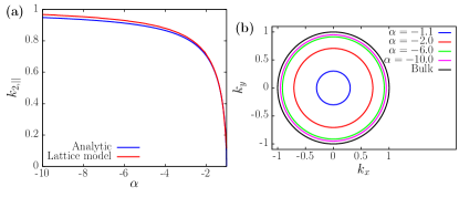
Figure 2: (a) Radius of shadow state Fermi circle $k_{2,||}$ versus the NNN hybridization strength $\alpha$ as determined from the numerical and analytical solutions of $H_{T}$. (b) Evolution of the shadow state FS with $\alpha$. The black line corresponds to the extremal-area section of the FS for the bulk unhybridized bands. For sufficiently large $\alpha$, the shadow state FS becomes comparable to the extremal area of the bulk unhybridized bands. The shadow state solutions were obtained for $\beta=0$ and all remaining parameters are the same as in Fig. 1.

For $\beta=0$, the FS, which is circularly symmetric for the chosen parameters with radius $k_{2,||}$ , corresponds to the crossing points of the two surface bands. For non-zero $\beta$, a gap opens on the surface-state FS, except for 8 points located at $\theta_{k}=m\pi/2$ and $\theta_{k}=\pi/4+m\pi/2$ ($m$ is integer and $\tan\theta_{k}=k_{y}/k_{x}$). These correspond to surface Dirac points. We distinguish between Dirac points at $\theta_{k}=m\pi/2$ and $\theta_{k}=\pi/4+m\pi/2$. For $\theta_{k}=m\pi/2$ the Dirac points are located at $k_{2,||}=\sqrt{M/m+1/\alpha}$ (since $\beta$ dependent terms do not contribute when either $k_{x}$ or $k_{y}$ is zero), while for $\theta_{k}=\pi/4+m\pi/2$ the Dirac points occur at $k^{\prime}_{2,||}=\sqrt{\left(m+M\alpha\right)/m\alpha\left(1-\beta/2\right)}$. As $\beta$ increases beyond a critical value $\beta_{c}=2/|\alpha|k^{2}_{F}=2m/|\alpha|M$, the bulk gap closes for $\theta_{k}=\pi/4+m\pi/2$ and the corresponding surface Dirac points become gapped. This is confirmed by the numerical results shown in Fig. 1 (b-d). At $\beta=\beta_{c}$ the bulk band structure contains four 3D Dirac points located in the $k_{z}=0$ plane, along directions $\theta_{k}=\pi/4+m\pi/2$ and at distance $k_{F}$ from the center of the BZ as shown in Fig. 3. For $\beta>\beta_{c}$ the FS of the surface state consists of four Fermi points at directions $\theta_{k}=m\pi/2$.

Fig. 4 shows the evolution of the surface-state band gap and corresponding FS extracted from the numerical solutions as a function of $\beta$. There are two Lifshitz transitions between the bands in panels (a) and (b) and (c) and (d) , respectively, as the point-group symmetry is enhanced from tetragonal to cubic by increasing $\beta$.

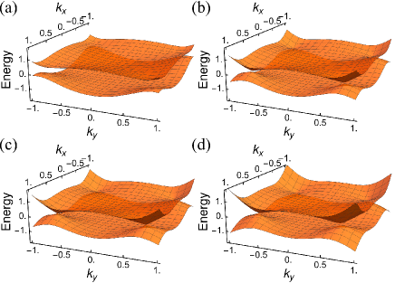
Figure 3: The bulk band structure for $\beta=0.2,0.3,1/3,0.4$ (a-d) at $k_{z}=0$. The remaining parameters are the same as in Fig. 1. For current parameters $\beta_{c}=1/3$.

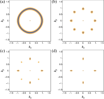
Figure 4: Density plot of the surface-state gap determined from the numerical solutions for $\beta=0.0,0.2,0.3,0.35$ (a-d) respectively. The remaining parameters are the same as in Fig. 1.

Quantum oscillations induced by the shadow surface states

The presence of shadow surface states with finite FS’s at charge neutrality, which emerge in the extreme limit where $\beta=0$, manifests in QO of the magnetization for arbitrarily small fields. For small NNN in-plane hybridization ($\beta>0$), the surface states become gapped except at an odd number of Dirac points. Provided that the gap is sufficiently small compared to the LL spacing, QO can still occur. Note that the surface state gap is tuned by the anisotropy parameter $\beta$ and can, in principle, be made arbitrarily small. In the most general case, QO from the surface states can thus occur for fields well below the threshold for QO from the gapped bulk. To show that this is the case, we calculated the magnetization of the ground state as a function of a magnetic field $B$ applied in a direction perpendicular to the surface for a set of values of the chemical potential $\mu$ and anisotropy parameter $\beta$. The results are shown in Fig. 5. Here, $E_{g}$ is the minimum value of the direct gap of the bulk states, while $\hbar\omega_{B}$ is the LL spacing for the unhybridized itinerant electron band in the presence of the field $B$. The ratio $E_{g}/\hbar\omega_{B}$ provides a threshold for QO from the gapped bulk. Indeed, this ratio decreases with increasing field and we expect QO from the gapped bulk whenever it drops below unity. By contrast, we observe QO from the surface states at ratios well above unity, or correspondingly for fields well below the threshold value for the bulk, as illustrated in the figure.

We now turn to a detailed discussion of the results. Note that the non-oscillating part of the magnetization was subtracted. Panels (a) and (b) of Fig. 5 show the QO for $\mu=0$ and for two values of the anisotropy parameter $\beta$. When $\beta=0$ we observe QO for all of the values of the ratio $E_{g}/\hbar\omega_{B}$, which are well away from the O(1) threshold value for QO from the gapped bulk. Note that the frequency of the oscillations is comparable to that of the unhybridized bulk bands FS for the same magnetic field B. For finite $\beta$, sharp QO are observed only for lower values of $E_{g}/\hbar\omega_{B}$ corresponding to higher fields. Due to the presence of a gap in surface state spectrum stronger magnetic fields are needed to observe quantum oscillations due to the magnetic breakdown.

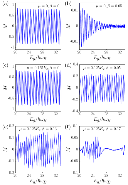
Figure 5: The QO of the magnetization at zero temperature for a set of values for the chemical potential and anisotropy parameter $\beta$. As discussed in the text, the ratio of the minimum direct bulk gap $E_{g}$ and the LL spacing of the unhybridized itinerant electron band $\hbar\omega_{B}$ for given magnetic field $B$ provides a measure of the contributions to the magnetic oscillations from the gapped bulk. The latter become important for $E_{g}/\hbar\omega_{B}\ll 1$. By contrast, we observe QO well above this threshold, due to the contribution of the surface states Note that the chemical potential is always in the bulk gap.All other parameters are the same as in Fig. 1

We also consider the magnetization for a finite value of $\mu$ for increasing values of $\beta$ in Fig. 5 (c)-(f). When both $\mu$ and $\beta$ are finite, a finite FS consisting of 8 small pockets emerges, as shown in Fig. 4. The contribution of these small pockets , which oscillates with a lower frequency, becomes discernible with increasing $\beta$, as seen in panels (e) and (f).

These results illustrate that, close to the limit where the NNN in-plane hybridization vanishes, QO from the surface states with a frequency comparable to that of the bulk bands are clearly seen for magnetic fields well below the threshold for QO from the gapped bulk.

One aspect of quantum oscillation, which is used to identify the two dimensional nature of conducting states, is the dependence of the frequency of oscillations on the tilt angle of the magnetic field. In conventional 2D electronic systems, the frequency of magnetic oscillations depends on the cross-sectional area of the Fermi surface normal to the field direction. This is related to the field component in the direction normal to the surface. For the shadow states, in addition to such dependence on the magnetic field direction, tilting of the field leads to gaping of the states and suppresses the magnetic oscillations. This is demonstrated numerically for the lattice model in Fig. 6. This effect results from hybridization of the two surface states due to the in plane component of the field and occurs at the Fermi energy where the bands cross. As a result, the effect of tilting of magnetic field can be used to distinguish the the surface states in this paper from other types of edge states.

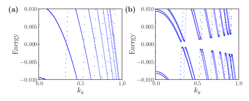
Figure 6: Gaping of the edge states in the presence of the in plane field. (a) and (b) corresponds to $\hbar\omega_{B\parallel}=0$ and $\hbar\omega_{B\parallel}=0.025$. The results are obtained for 2D lattice in $xz$ plane with $50\times 50$ sites and applying periodic boundary conditions in $x$ direction. $\beta=0$ and all the remaining parameters are the same as in Fig. 1.

III Lattice models and interaction-induced shadow states

The emergence of shadow states in the effective continuum model requires $\alpha<-m/M$. It is crucial to examine which microscopic model could lead to effective models as in (1) and (3) and illustrate how these microscopic models map onto the continuum limit discussed in Sec. II. In particular, such microscopic models involve small ratios of NN to NNN hybridizations which would be highly atypical of direct orbital overlaps in a non-interacting model. In this section we show that such hybridization structure can emerge as a result of strong interactions in TKIs.

The kinetic part of continuum model in (1) corresponds to the following form in the lattice model:

$$\begin{split}H_{k}=&\left[\left(M^{\prime}-6m^{\prime}\right)+2m^{\prime}\sum_{i}\cos\left(k_{i}a\right)\right]\left(f_{\textbf{k}}^{\dagger}f_{\textbf{k}}+c_{\textbf{k}}^{\dagger}c_{\textbf{k}}\right)+\\ &\left[\left(M-6m\right)+2m\sum_{i}\cos\left(k_{i}a\right)\right]\left(f_{\textbf{k}}^{\dagger}f_{\textbf{k}}-c_{\textbf{k}}^{\dagger}c_{\textbf{k}}\right),\end{split}$$ (8)

where $f_{\textbf{k}}$ and $c_{\textbf{k}}$ are destruction operators associated with localized and itinerant bands. For simplicity we choose half-filled localized band limit. Away from $f$-electron half-filling requires mole elaborate discussion of the interacting model (see Section III.4) which will be presented elsewhere. We should note that even though the localized $f$ band is at half-filling, the effective Heisenberg interaction between the localized moments leads to an effective dispersion for the bandSenthil et al. (2004a); Alexandrov et al. (2015); Ghaemi and Senthil (2007).

III.1 General form of the effective hybridization in a lattice model

We consider an effective $s-p$ orbital hybridization on a three-dimensional lattice in the presence of spin-orbit coupling with the most general tetragonal point-group symmetry. The form of these effective hybridization terms is determined by the point-group symmetry and does not depend on strong correlations. However, as we discuss in the next section, the effective hybridization gets renormalized due to strong correlations. We consider a general form which allows for tetragonal anisotropy. The NN and NNN, symmetry-allowed hybridization terms, which include the spin-orbit coupling, in second-quantized form areColeman (2015)

$$H_{\text{Hyb}}= \sum_{\mathbf{R},\mu}\bigg{[}t_{0\parallel}\left(f^{{\dagger}}_{\mathbf{R}\mu}\Psi_{0\parallel,\mathbf{R}\mu}+\text{H.c.}\right)+t_{0\perp}\left(f^{{\dagger}}_{\mathbf{R}\mu}\Psi_{0\perp,\mathbf{R}\mu}+\text{H.c.}\right)+t_{1\parallel}\left(f^{{\dagger}}_{\mathbf{R}\mu}\Psi_{1\parallel,\mathbf{R}\mu}+\text{H.c.}\right)+t_{1\perp}\left(f^{{\dagger}}_{\mathbf{R}\mu}\Psi_{1\perp,\mathbf{R}\mu}+\text{H.c.}\right)\bigg{]},$$ (9)

where $\mathbf{R}$ labels the sites of the cubic lattice and the $f^{{\dagger}}_{\mathbf{R}\mu}$ operator acts on the lowest-energy Kramers doublet which emerges under the effect of the cubic or tetragonal crystal field from the $p$-orbital with spin $1/2$. Since the spin in not conserved, $\mu\in\{1,2\}$ denotes the two components of the Kramers doublet. We introduced the Wannier states

$$\Psi_{0\parallel,\mathbf{R}\mu}= -\frac{i}{2}\sum_{\mathbf{\hat{r}}\in\{\pm\mathbf{\hat{x}},\pm\mathbf{\hat{y}}\}}\sum_{\nu}\left(\mathbf{\hat{r}}\cdot\mathbf{\sigma}\right)_{\mu\nu}c_{\mathbf{R}+\mathbf{\hat{r}}\nu}$$ (10)

$$\Psi_{0\perp,\mathbf{R}\mu}= -\frac{i}{2}\sum_{\mathbf{\hat{r}}\in\{\pm\mathbf{\hat{z}}\}}\sum_{\nu}\left(\mathbf{\hat{r}}\cdot\mathbf{\sigma}\right)_{\mu\nu}c_{\mathbf{R}+\mathbf{\hat{r}}\nu}$$ (11)

$$\Psi_{1\parallel,\mathbf{R}\mu}= -\frac{i}{2}\sum_{\mathbf{\hat{r}}\in\{\pm\mathbf{\hat{x}}\pm\mathbf{\hat{y}}\}}\sum_{\nu}\left(\mathbf{\hat{r}}\cdot\mathbf{\sigma}\right)_{\mu\nu}c_{\mathbf{R}+\mathbf{\hat{r}}\nu}$$ (12)

$$\Psi_{1\perp,\mathbf{R}\mu}= -\frac{i}{2}\sum_{\mathbf{\hat{r}}\in\begin{subarray}{c}\{\pm\mathbf{\hat{x}}\pm\mathbf{\hat{z}},\\ \pm\mathbf{\hat{y}}\pm\mathbf{\hat{z}}\}\end{subarray}}\sum_{\nu}\left(\mathbf{\hat{r}}\cdot\mathbf{\sigma}\right)_{\mu\nu}c_{\mathbf{R}+\mathbf{\hat{r}}\nu},$$ (13)

defined in terms of the $s$-orbital, spin-$1/2$ conduction electrons $c_{\mathbf{R}\nu}$. By construction, each of $\Psi$’s belong to the same doublet as the $f$ fermion operators. For the most general tetragonal anisotropy, the NN hybridization splits into in-plane $t_{0\parallel}$ and out-of-plane $t_{0\perp}$ contributions, and similarly for the NNN terms $t_{1\parallel}$ and $t_{1\perp}$. Under a straightforward Fourier transformation, the hybridization terms can be re-expressed as:

$$H_{\text{Hyb}}= \sum_{\mathbf{k},\mu\nu}\bigg{[}V_{0,\mu\nu}(\mathbf{k})+V_{1,\mu\nu}(\mathbf{k})\bigg{]}f^{{\dagger}}_{\mathbf{k}\mu}c_{\mathbf{k}\nu}+\text{H.c.}$$ (14)

where

$$V_{0,\mu\nu}(\mathbf{k})= t_{0\parallel}\sum_{i\in\{x,y\}}s_{i}\sigma_{i,\mu\nu}+t_{0\perp}\sigma_{z,\mu\nu}s_{z}$$ (15)

$$V_{1,\mu\nu}(\mathbf{k})= 2\bigg{[}\left(t_{1\parallel}c_{y}+t_{1\perp}c_{z}\right)s_{x}\sigma_{x}+\left(t_{1\parallel}c_{x}+t_{1\perp}c_{z}\right)s_{y}\sigma_{y}$$

$$+t_{1\perp}\left(c_{x}+c_{y}\right)s_{z}\sigma_{z}\bigg{]}$$ (16)

and where $s_{i}=\sin(k_{i}a),c_{i}=\cos(k_{i}a)$.

III.2 Continuum limit for cubic symmetry

For cases where the hybridization preserves the cubic point-group symmetry we set $t_{0\parallel}=t_{0\perp}$ and $t_{1\parallel}=t_{1\perp}$. Taking the continuum limit of the hybridization terms in (15) and (16) we arrive at (1) and (3) for $\beta=1$ by identifying

$$v =t_{0}+4t_{1}$$ (17)

$$\alpha v =-t_{1},$$ (18)

from which the condition for the emergence of shadow states, $\alpha<-m/M$, translates into

$$-4t_{1}<t_{0}<\left(\frac{M}{m}-4\right)t_{1}\quad\mathrm{if}\,t_{1}>0$$ (19)

$$\left(\frac{M}{m}-4\right)t_{1}<t_{0}<-4t_{1}\quad\qquad\mathrm{if}\,t_{1}<0.$$ (20)

III.3 Continuum limit for tetragonal symmetry

The parameters of the continuum model in (1) and (3) are related to the lattice model parameters in (15) and 16 via:

$$v_{\parallel} =2t_{1\parallel}+2t_{1\perp}+t_{0\parallel},$$ (21)

$$v_{\perp} =t_{0\perp}+4t_{1\perp},$$ (22)

$$\alpha =\frac{-t_{1\perp}}{t_{0\perp}+4t_{1\perp}},$$ (23)

$$\beta =\frac{t_{1\parallel}}{t_{1\perp}},$$ (24)

where $v_{\parallel}$ ($v_{\perp}$) is the hybridization amplitude in the $xy$ plane and along the $z$ direction, respectively in (1). As mentioned previously, the anisotropy of the NN hybridization does not have essential consequences .

For tetragonal lattices, the condition for the surface state crossings at finite parallel momentum (the equivalent of (7) when $v_{\parallel}\neq v_{\perp}$) reads as $\frac{\alpha v_{\perp}}{v_{\parallel}}<-\frac{m}{M}$. In terms of parameters of tight-binding, the required range of tight-binding model parameters read as:

$$\frac{-t_{1\perp}}{2t_{1\parallel}+2t_{1\perp}+t_{0\parallel}}<-\frac{m}{M}.$$ (25)

For $\beta=0$ ($t_{1\parallel}=0$), this condition implies

$$-2t_{1\perp}<t_{0\parallel}<\left(\frac{M}{m}-2\right)t_{1\perp}\quad\mathrm{if}\,t_{1\perp}>0$$ (26)

$$\left(\frac{M}{m}-2\right)t_{1\perp}<t_{0\parallel}<-2t_{1\perp}\quad\mathrm{if}\,t_{1\perp}<0.$$ (27)

This shows that if $k^{2}_{F}=M/m<2$ the emergence of shadow states requires that $t_{0\parallel}$ and $t_{1\perp}$ have opposite signs. Recall that this conclusion is a consequence of (25), and is therefore rigorous only in the continuum limit when $M/m<1$. We note that for larger values of $M/m$, shadow states could develop even if $t_{0\parallel}$ and $t_{1\perp}$ have the same sign. This case corresponds to very large shadow surface state FSs and is consequently relevant in a restricted parameter-space. Therefore, we focus on $t_{0\parallel}$ and $t_{1\perp}$ having opposite sign. In Sec.III.4 we demonstrate that for TKIs and due to the interacting nature of this material, such emergent pattern of parameters is energetically preferred.

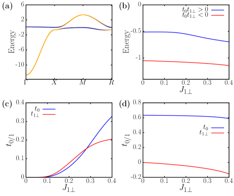
Figure 7: (a) Band structure determined from (38), (39) and (14) for the self-consistent solutions with effective $f$-electron level $\mu_{f}=0.66$, and NN and NNN hybridization $t_{0}=0.62$ and $t_{1}=-0.08$, respectively, which corresponds to $J_{1\perp}=0.3$. Yellow (blue) lines denote $c(f)$ character. (b) Ground-state energy per unit cell versus NNN Kondo coupling $J_{1\perp}$ for solutions where the NN and NNN effective hybridizations $t_{0}$ and $t_{1\perp}$, respectively, have equal (blue line) and opposite (red line) signs. The lowest-energy ground-state configuration occurs when the signs are opposite. Self-consistently determined NN and NNN effective hybridizations $t_{0}$ and $t_{1\perp}$, respectively, as functions of the NNN Kondo-coupling $J_{1\perp}$ for (c) $t_{0}t_{1\perp}>0$ and (d) $t_{0}t_{1\perp}<0$. The values of the parameters are: $t=1.0$, $t^{\prime}=0.5$, $J_{0\parallel}=J_{0\perp}=1.0$ and $J_{1\parallel}=0$, which correspond to $t_{0\parallel}=t_{0\perp}=t_{0}$ and $t_{1\parallel}=0$.

III.4 Effective hybridization from Kondo interactions

The Kondo interaction, effectively emerges from Anderson model at half-filling of localized fermionic band in the large interaction limit between electrons occupying the same localized orbital Coleman (2015); Hewson (1993). Kondo lattice model can be derived as a lower energy effective model from periodic Anderson model using Schrieffer–Wolff transformation Schrieffer and Wolff (1966). The resulting low energy Kondo model incorporates an interaction term which is of the form of anti-ferromagnetic coupling between the spin of electrons in the local band and the spin of itinerant electrons. Given that the Kondo model is still interacting we need to apply suitable treatment such as mean-field approximationColeman (2015); Ghaemi and Senthil (2007). Such treatments were used to capture phenomena such as large FS and heavy quasiparticle mass in heavy-Fermi liquidsSenthil et al. (2003, 2004b). In this section, we show that $t_{0\parallel}$ and $t_{1\perp}$ having opposite signs is energetically preferred at mean-field level for TKIs. In the half-filling limit, we consider the NN and NNN Kondo interactionDzero et al. (2016b); Alexandrov and Coleman (2014); Ghaemi and Senthil (2007); Ghaemi et al. (2008)

$$H_{K}= \sum_{\mathbf{R}}\bigg{[}J_{0\parallel}\mathbf{S}_{0\parallel,\mathbf{R}}\cdot\mathbf{S}_{f,\mathbf{R}}+J_{0\perp}\mathbf{S}_{0\perp,\mathbf{R}}\cdot\mathbf{S}_{f,\mathbf{R}}$$

$$+J_{1\parallel}\mathbf{S}_{1\parallel,\mathbf{R}}\cdot\mathbf{S}_{f,\mathbf{R}}+J_{1\perp}\mathbf{S}_{1\perp,\mathbf{R}}\cdot\mathbf{S}_{f,\mathbf{R}}\bigg{]}$$ (28)

where

$$\mathbf{S}_{f,\mathbf{R}}= \frac{1}{2}\sum_{\mu\nu}f^{{\dagger}}_{\mathbf{R}\mu}\mathbf{\sigma}_{\mu\nu}f_{\mathbf{R}\nu}.$$ (29)

For tetragonal symmetry, the in-plane and out-of-plane Kondo couplings are different with $J_{0/1\parallel}\neq J_{0/1\perp}$. Note that the $f$ fermion is constrained to the half-filled Fock space. Similarly, the operators

$$\mathbf{S}_{0\parallel,\mathbf{R}}= \frac{1}{2}\sum_{\mu\nu}\Psi^{{\dagger}}_{0\parallel,\mathbf{R}\mu}\mathbf{\sigma}_{\mu\nu}\Psi_{0\parallel,\mathbf{R}\nu}$$ (30)

$$\mathbf{S}_{0\perp,\mathbf{R}}= \frac{1}{2}\sum_{\mu\nu}\Psi^{{\dagger}}_{0\perp,\mathbf{R}\mu}\mathbf{\sigma}_{\mu\nu}\Psi_{0\perp,\mathbf{R}\nu}$$ (31)

$$\mathbf{S}_{1\parallel,\mathbf{R}}= \frac{1}{2}\sum_{\mu\nu}\Psi^{{\dagger}}_{1\parallel,\mathbf{R}\mu}\mathbf{\sigma}_{\mu\nu}\Psi_{1\parallel,\mathbf{R}\nu}$$ (32)

$$\mathbf{S}_{1\perp,\mathbf{R}}= \frac{1}{2}\sum_{\mu\nu}\Psi^{{\dagger}}_{1\perp,\mathbf{R}\mu}\mathbf{\sigma}_{\mu\nu}\Psi_{1\perp,\mathbf{R}\nu}$$ (33)

are defined in terms of the Wannier states in (10)-(13).

A straightforward decoupling of the Kondo interactions in the particle-hole channel reproduces (14) if we identify

$$t_{0\parallel}= -\frac{3J_{0\parallel}}{8}\bigg{\langle}\sum_{\mu}\Psi^{{\dagger}}_{0\parallel,\mathbf{R}\mu}f_{\mathbf{R}\mu}\bigg{\rangle}$$ (34)

$$t_{0\perp}= -\frac{3J_{0\perp}}{8}\bigg{\langle}\sum_{\mu}\Psi^{{\dagger}}_{0\perp,\mathbf{R}\mu}f_{\mathbf{R}\mu}\bigg{\rangle}$$ (35)

$$t_{1\parallel}= -\frac{3J_{1\parallel}}{8}\bigg{\langle}\sum_{\mu}\Psi^{{\dagger}}_{1\parallel,\mathbf{R}\mu}f_{\mathbf{R}\mu}\bigg{\rangle}$$ (36)

$$t_{1\perp}= -\frac{3J_{1\perp}}{8}\bigg{\langle}\sum_{\mu}\Psi^{{\dagger}}_{1\perp,\mathbf{R}\mu}f_{\mathbf{R}\mu}\bigg{\rangle}$$ (37)

We choose a tight-binding part for conduction and $f$ electrons Alexandrov et al. (2015):

$$\epsilon_{\mathbf{k}} =-2t\sum_{i}\cos k_{i}-4t^{\prime}\sum_{i\neq j}\cos k_{i}\cos k_{j},$$ (38)

$$\epsilon_{\mathbf{fk}} =-\eta\epsilon_{\mathbf{k}}+\mu_{f},$$ (39)

where $\eta=0.01$ and $\mu_{f}$ is the chemical potential for the $f$ electrons. We impose half-filling for both f and conduction electrons:

$$1 =\frac{1}{N_{k}}\langle\sum_{\mathbf{k}\mu}f^{\dagger}_{\mathbf{k}\mu}f_{\mathbf{k}\mu}\rangle,$$ (40)

$$1 =\frac{1}{N_{k}}\langle\sum_{\mathbf{k}\mu}c^{\dagger}_{\mathbf{k}\mu}c_{\mathbf{k}\mu}\rangle,$$ (41)

where $N_{k}$ is the number of points in the bulk BZ. Finally, both $t_{i\parallel/\perp}$ and $\mu_{f}$ are determined self-consistently.

Fig. 7 (a) shows the band structure of the Hamiltonian formed from (38), (39) and (14). The ground state has band inversion at the 3 $M$ points in the in the BZ and therefore has a nontrivial topological Z₂ index. Fig. 7 (b-d) shows the solution of (34-37) for half-filling, when $t_{0}=t_{0\parallel}=t_{0\perp}$ and $t_{1\parallel}=0$. We distinguish solutions with $t_{0}$ and $t_{1\perp}$ having the same and opposite sign. We find that the self-consistent solutions with $t_{0}t_{1\perp}<0$ minimize the ground-state energy whereas solutions with $t_{0}t_{1\perp}>0$ are always higher in energy as shown in Fig. 7 (b). Fig. 7 (c) and (d) show the corresponding $t_{0/1\perp}$ as a function of $J_{1}$ for $J_{0}$ = 1. At $J_{1}=0$ the lower energy solution corresponds to finite $t_{0}$ and $t_{1\perp}=0$. Moving away to finite $J_{1}$ the $t_{0}t_{1\perp}<0$ solution smoothly connects with that low energy solution, whereas $t_{0}t_{1\perp}>0$ solution develops in different region and is never preferred.

IV Conclusions

Motivated by the well-studied case of SmB₆, we considered a natural extension of a minimal two-orbital model with NN hybridization for cubic TKIs to cases with tetragonal anisotropy and additional NNN hybridization. In the tetragonal limit with strictly NNN out-of-plane hybridization, we found that the surface states show two FS’s with different effective masses at the charge neutrality point. The existence of two FS’s, one hole-like and another electron-like, with equal areas but very different effective masses is inherent to TKI’s, due to the hybridization between quasi-localized and itinerant electrons. These features, in turn make finite-frequency QO possible. This contrasts with the more common situation in TI’s, which typically exhibit Dirac points at charge neutrality and no QO from the surface states for vanishing magnetic fields. The QO due to the surface states can also occur in presence of finite NNN in-plane hybridization or disorder, provided that the gaps induced by these mechanisms are comparable to the Landau level spacing.

In addition, we showed that a predominantly NNN out-of-plane hybridization realizes the minimum-energy ground-state configuration in TKIs with tetragonal lattice symmetry. Consequently, shadow surface states provide a concrete example of how arbitrarily high-frequency QO can occur beyond the immediate context of cubic TKIs such as SmB₆.

Finally, we note that the ideal candidates for the emergence of shadow surface states with a small gap are compounds with a dominant NNN out-of plane hybridization. The most natural realizations are therefore topological Kondo insulators under strong compressive strain.

V Appendix

In this appendix, we discuss the analytical solutions of the surface states of continuum-limit Hamiltonian $H_{T}=H_{0}+V_{nnn}$ introduced in Sec. II. Taking into account the double-degeneracy of the states due to inversion and time-reversal symmetry, we consider the following two degenerate eigenstates ansatz for the general solutions of $H_{T}$ (in the basis $\left\{|1,\uparrow\rangle,|2,\uparrow\rangle,|1,\downarrow\rangle,|2,\downarrow\rangle\right\}$, $\{1,2\}$ denoting orbital index and $\{\uparrow,\downarrow\}$ denoting the spin):

$$\psi^{1}_{\xi}(z)=N_{1}\left(\begin{array}[]{c}L_{-}+m_{-}\lambda^{2}_{\xi}-E\\ iv\lambda_{\xi}\left(1+\alpha k^{2}\right)\\ 0\\ -vk_{x}\left(1+\alpha\left(\beta k^{2}_{y}-\lambda^{2}_{\xi}\right)\right)-ivk_{y}\left(1+\alpha\left(\beta k^{2}_{x}-\lambda^{2}_{\xi}\right)\right)\end{array}\right)e^{-\lambda_{\xi}z},$$ (42)

$$\psi^{2}_{\xi}(z)=N_{2}\left(\begin{array}[]{c}-vk_{x}\left(1+\alpha\left(\beta k^{2}_{y}-\lambda^{2}_{\xi}\right)\right)+ivk_{y}\left(1+\alpha\left(\beta k^{2}_{x}-\lambda^{2}_{\xi}\right)\right)\\ 0\\ -iv\lambda_{\xi}\left(1+\alpha k^{2}\right)\\ L_{+}+m_{+}\lambda^{2}_{\xi}-E\end{array}\right)e^{-\lambda_{\xi}z},$$ (43)

where $L_{\pm}=M_{\pm}-m_{\pm}k^{2}_{\parallel}$, $M_{\pm}=M^{\prime}\pm M$, $m_{\pm}=m^{\prime}\pm m$, $\xi=1,2$ and $\lambda_{\xi}$ are determined from a characteristic equationShan et al. (2010); Shen (2012). We focus on non-trivial surface states of a semi-infinite system with an open boundary condition at $z=0$ and normalization condition of the wave function in the region $z>0$. Therefore, we are only interested in $\lambda_{\xi}$ with positive real part. Using the definitions

$$F =m_{+}\left(L_{-}-E\right)+m_{-}\left(L_{+}-E\right)$$

$$+v^{2}\left(1+4\alpha k_{\parallel}^{2}+\alpha^{2}k_{\parallel}^{4}+4\alpha^{2}\beta k^{2}_{x}k^{2}_{y}\right)$$ (44)

$$R =F^{2}-4\left(m_{+}m_{-}-\alpha^{2}v^{2}k_{\parallel}^{2}\right)\times$$

$$\left[\left(L_{+}-E\right)\left(L_{-}-E\right)-v^{2}\left(k_{\parallel}^{2}+\alpha\beta k^{2}_{x}k^{2}_{y}\left(4+\alpha\beta k_{\parallel}^{2}\right)\right)\right]$$ (45)

we express the solutions via

$$\lambda_{\xi} =\left[2\left(m_{+}m_{-}-\alpha^{2}v^{2}k_{\parallel}^{2}\right)\right]^{-\frac{1}{2}}\times$$

$$\hskip 60.0pt\left(-F+(-1)^{\xi}\sqrt{R}\right)^{\frac{1}{2}}$$ (46)

Non-trivial solution satisfying boundary condition at $z=0$ are obtained from the requirement $\det\{\psi^{1}_{1}(0),\psi^{1}_{2}(0),\psi^{2}_{1}(0),\psi^{2}_{2}(0)\}=0$, which takes simple form at $k_{2,||}$ when $\beta=0$ or $\theta_{k}=m\pi/2$:

$$\lambda_{1}\lambda_{2}=-\frac{1}{\alpha},$$ (47)

For $\beta\neq 0$, and $\theta_{k}=\pi/4+m\pi/2$ also for $k^{\prime}_{2,||}$, the condition is

$$\lambda_{1}\lambda_{2}=\frac{1}{\beta-2}\left(\frac{M\beta}{m}+\frac{2}{\alpha}\right).$$ (48)

Non-trivial surface states thus require $\lambda_{1}\lambda_{2}>0$ and since $0<\beta<1$, the above conditions can only be satisfied if $\alpha<0$. In addition, the condition (48) requires $\alpha>-2m/M\beta$ which is equivalent to $\beta<\beta_{c}$ derived in main text.

For general momentum $k_{||}$, the non-trivial surface state spectrum is

$$E_{\pm}= \frac{M^{\prime}m^{2}-Mmm^{\prime}}{m^{2}+\alpha^{2}v^{2}k_{\parallel}^{2}}+\frac{\alpha v^{2}\left(m^{\prime}k_{\parallel}^{2}+\alpha\left(M^{\prime}-m^{\prime}k_{\parallel}^{2}\right)k_{\parallel}^{2}+2\alpha\beta m^{\prime}k^{2}_{x}k^{2}_{y}\right)}{m^{2}+\alpha^{2}v^{2}k_{\parallel}^{2}}\pm$$

$$\frac{v}{m^{2}+\alpha^{2}v^{2}k_{\parallel}^{2}}\left[\left(m^{2}-m^{\prime 2}+\alpha^{2}v^{2}k_{\parallel}^{2}\right)\left(\left(m+\alpha\left(M-mk_{\parallel}^{2}\right)\right)^{2}k_{\parallel}^{2}+\alpha^{2}\beta^{2}m^{2}k^{2}_{x}k^{2}_{y}k_{\parallel}^{2}+\right.\right.$$

$$\left.\left.4\alpha\beta mk^{2}_{x}k^{2}_{y}\left(m+\alpha\left(M-mk_{\parallel}^{2}\right)\right)+\alpha^{4}\beta^{2}v^{2}k^{2}_{x}k^{2}_{y}\left(k^{2}_{x}-k^{2}_{y}\right)^{2}\right)\right]^{1/2}.$$ (49)

Above spectrum reduces to the from given in (4) for $\beta=0$.

References

- Fisk et al. (1995) Z. Fisk, J. L. Sarrao, J. D. Thompson, D. Mandrus, M. F. Hundley, A. Migliori, B. Bucher, Z. Schlessinger, G. Aeppli, E. Bucher, J. F. DiTusa, C. S. Oglesby, H.-R. Ott, P. C. Canfield, and S. E. Brown, Physica B 206 & 207, 798 (1995).
- Menth et al. (1969) A. Menth, E. Buehler, and T. H. Geballe, Phys. Rev. Lett. 22, 295 (1969).
- Dzero et al. (2010) M. Dzero, K. Sun, V. Galitski, and P. Coleman, Phys. Rev. Lett. 104, 106408 (2010).
- Dzero et al. (2012) M. Dzero, K. Sun, P. Coleman, and V. Galitski, Phys. Rev. B 85, 045130 (2012).
- Alexandrov et al. (2013) V. Alexandrov, M. Dzero, and P. Coleman, Phys. Rev. Lett. 111, 226403 (2013).
- Dzero et al. (2016a) M. Dzero, J. Xia, V. Galitski, and P. Coleman, Annu. Rev. Condens. Matter Phys. 7, 249 (2016a).
- Jiang et al. (2013) J. Jiang, S. Li, T. Zhang, Z. Sun, F. Chen, Z. Ye, M. Xu, Q. Ge, S. Tan, X. Niu, M. Xia, B. Xie, Y. Li, X. Chen, H. Wen, and D. Feng, Nat. Comm. 4, 3010 (2013).
- Kim et al. (2014) D. J. Kim, J. Xia, and Z. Fisk, Nature Materials 13, 466 (2014).
- Neupane et al. (2013) M. Neupane, N. Alidoust, S.-Y. Xu, T. Kondo, Y. Ishida, D. J. Kim, C. Liu, I. Belopolski, Y. J. Jo, T.-R. Chang, H.-T. Jeng, T. Durakiewicz, L. Balicas, H. Lin, A. Bansil, S. Shin, Z. Fisk, and M. Z. Hasan, Nat. Comm. 4, 2991 (2013).
- Frantzeskakis et al. (2013) E. Frantzeskakis, N. de Jong, B. Zwartsenberg, Y. K. Huang, Y. Pan, X. Zhang, J. X. Zhang, F. X. Zhang, L. H. Bao, O. Tegus, A. Varykhalov, A. de Visser, and M. S. Golden, Phys. Rev. X 3, 041024 (2013).
- Denlinger et al. (2014) J. D. Denlinger, J. W. Allen, J.-S. Kang, K. Sun, B.-I. Min, D.-J. Kim, and Z. Fisk, “Smb¡sub¿6¡/sub¿ photoemission: Past and present,” in Proceedings of the International Conference on Strongly Correlated Electron Systems (SCES2013) (2014) p. 017038.
- Xu et al. (2016) N. Xu, H. Ding, and M. Shi, Journal of Physics: Condensed Matter 28, 363001 (2016).
- Phelan et al. (2014) W. A. Phelan, S. M. Koohpayeh, P. Cottingham, J. W. Freeland, J. C. Leiner, C. L. Broholm, and T. M. McQueen, Phys. Rev. X 4, 031012 (2014).
- Laurita et al. (2016) N. J. Laurita, C. M. Morris, S. M. Koohpayeh, P. F. S. Rosa, W. A. Phelan, Z. Fisk, T. M. McQueen, and N. P. Armitage, Phys. Rev. B 94, 165154 (2016).
- Li et al. (2014) G. Li, Z. Xiang, F. Yu, T. Asaba, B. Lawson, P. Cai, C. Tinsman, A. Berkley, S. Wolgast, Y. S. Eo, D.-J. Kim, C. Kurdak, J. W. Allen, K. Sun, X. H. Chen, Y. Y. Wang, Z. Fisk, and L. Li, Science 346, 1208 (2014).
- Tan et al. (2015) B. Tan, Y.-T. Hsu, B. Zeng, M. C. Hatnean, N. Harrison, Z. Zhu, M. Hartstein, M. Kiourlappou, A. Srivastava, M. Johannes, T. P. Murphy, J.-H. Park, L. Balicas, G. G. Lonzarich, G. Balakrishnan, and S. E. Sebastian, Science 349, 287 (2015).
- Hartstein et al. (2018) M. Hartstein, W. Toews, Y.-T. Hsu, B. Zeng, X. Chen, M. C. Hatnean, Q. Zhang, S. Nakamura, A. Padgett, G. Rodway-Gant, J. Berk, M. K. Kingston, G. H. Zhang, M. K. Chan, S. Yamashita, T. Sakakibara, Y. Takano, J.-H. Park, L. Balicas, N. Harrison, N. Shitsevalova, G. Balakrishnan, G. G. Lonzarich, R. W. Hill, M. Sutherland, and S. E. Sebastian, Nature Physics 14, 166 (2018).
- Hartstein et al. (2020) M. Hartstein, H. Liu, Y.-T. Hsu, B. S. Tan, M. C. Hatnean, G. Balakrishnan, and S. E. Sebastian, arXiv preprint arXiv:2007.01453 (2020).
- Liu et al. (2018) H. Liu, M. Hartstein, G. J. Wallace, A. J. Davies, M. C. Hatnean, M. D. Johannes, N. Shitsevalova, G. Balakrishnan, and S. E. Sebastian, Journal of Physics: Condensed Matter 30, 16LT01 (2018).
- Xiang et al. (2018) Z. Xiang, Y. Kasahara, T. Asaba, B. Lawson, C. Tinsman, L. Chen, K. Sugimoto, S. Kawaguchi, Y. Sato, G. Li, S. Yao, Y. L. Chen, F. Iga, J. Singleton, Y. Matsuda, and L. Li, Science 362, 65 (2018).
- Knolle and Cooper (2015) J. Knolle and N. R. Cooper, Phys. Rev. Lett. 115, 146401 (2015).
- Zhang et al. (2016) L. Zhang, X.-Y. Song, and F. Wang, Phys. Rev. Lett. 116, 046404 (2016).
- Knolle and Cooper (2017) J. Knolle and N. R. Cooper, Phys. Rev. Lett. 118, 096604 (2017).
- Shen and Fu (2018) H. Shen and L. Fu, Physical review letters 121, 026403 (2018).
- Skinner (2019) B. Skinner, Phys. Rev. Materials 3, 104601 (2019).
- Pal (2017) H. K. Pal, Physical Review B 95, 085111 (2017).
- Peters et al. (2019) R. Peters, T. Yoshida, and N. Kawakami, Physical Review B 100, 085124 (2019).
- Lu et al. (2020) Y.-W. Lu, P.-H. Chou, C.-H. Chung, T.-K. Lee, and C.-Y. Mou, Physical Review B 101, 115102 (2020).
- Baskaran (2015) G. Baskaran, ArXiv e-prints (2015), arXiv:1507.03477 .
- Erten et al. (2017) O. Erten, P.-Y. Chang, P. Coleman, and A. M. Tsvelik, Phys. Rev. Lett. 119, 057603 (2017).
- Chowdhury et al. (2018) D. Chowdhury, I. Sodemann, and T. Senthil, Nat Commun. 9, 1766 (2018).
- Varma (2020) C. M. Varma, arXiv , 2008.07042 (2020).
- Alexandrov et al. (2015) V. Alexandrov, P. Coleman, and O. Erten, Phys. Rev. Lett. 114, 177202 (2015).
- Erten et al. (2016) O. Erten, P. Ghaemi, and P. Coleman, Phys. Rev. Lett. 116, 046403 (2016).
- Roy et al. (2014) B. Roy, J. D. Sau, M. Dzero, and V. Galitski, Phys. Rev. B 90, 155314 (2014).
- Poelchen et al. (2020) G. Poelchen, S. Schulz, M. Mende, M. Güttler, A. Generalov, A. V. Fedorov, N. Caroca-Canales, C. Geibel, K. Kliemt, C. Krellner, S. Danzenbächer, D. Y. Usachov, P. Dudin, V. N. Antonov, J. W. Allen, C. Laubschat, K. Kummer, Y. Kucherenko, and D. V. Vyalikh, npj Quantum Materials 5, 70 (2020).
- Wang et al. (2021) Y.-C. Wang, Y.-J. Xu, Y. Liu, X.-J. Han, X.-G. Zhu, Y.-f. Yang, Y. Bi, H.-F. Liu, and H.-F. Song, Phys. Rev. B 103, 165140 (2021).
- Han et al. (2019) Z. Han, T. Li, L. Zhang, G. Sullivan, and R.-R. Du, Phys. Rev. Lett. 123, 126803 (2019).
- Czajka et al. (2021) P. Czajka, T. Gao, M. Hirschberger, P. Lampen-Kelley, A. Banerjee, J. Yan, D. G. Mandrus, S. E. Nagler, and N. Ong, Nature Phys. , 1 (2021).
- Qi and Zhang (2011) X.-L. Qi and S.-C. Zhang, Rev. Mod. Phys. 83, 1057 (2011).
- Zhang et al. (2009) H. Zhang, C.-X. Liu, X.-L. Qi, X. Dai, Z. Fang, and S.-C. Zhang, Nature physics 5, 438 (2009).
- Liu et al. (2010) C.-X. Liu, X.-L. Qi, H. Zhang, X. Dai, Z. Fang, and S.-C. Zhang, Phys. Rev. B 82, 045122 (2010).
- Zhang et al. (2010) W. Zhang, R. Yu, H.-J. Zhang, X. Dai, and Z. Fang, New Journal of Physics 12, 065013 (2010).
- Shan et al. (2010) W.-Y. Shan, H.-Z. Lu, and S.-Q. Shen, New J. Phys. 12, 043048 (2010).
- Shen (2012) S.-Q. Shen, Topological insulators, Vol. 174 (Springer, 2012).
- Su et al. (1980) W. P. Su, J. R. Schrieffer, and A. J. Heeger, Phys. Rev. B 22, 2099 (1980).
- Senthil et al. (2004a) T. Senthil, M. Vojta, and S. Sachdev, Phys. Rev. B 69, 035111 (2004a).
- Ghaemi and Senthil (2007) P. Ghaemi and T. Senthil, Phys. Rev. B 75, 144412 (2007).
- Coleman (2015) P. Coleman, Introduction to many-body physics (Cambridge University Press, 2015).
- Hewson (1993) A. C. Hewson, The Kondo Problem to Heavy Fermions (Cambridge University Press, 1993).
- Schrieffer and Wolff (1966) J. R. Schrieffer and P. A. Wolff, Phys. Rev. 149, 491 (1966).
- Senthil et al. (2003) T. Senthil, S. Sachdev, and M. Vojta, Phys. Rev. Lett. 90, 216403 (2003).
- Senthil et al. (2004b) T. Senthil, M. Vojta, and S. Sachdev, Physical Review B 69, 035111 (2004b).
- Dzero et al. (2016b) M. Dzero, J. Xia, V. Galitski, and P. Coleman, Annual Review of Condensed Matter Physics 7, 249 (2016b).
- Alexandrov and Coleman (2014) V. Alexandrov and P. Coleman, Phys. Rev. B 90, 115147 (2014).
- Ghaemi et al. (2008) P. Ghaemi, T. Senthil, and P. Coleman, Phys. Rev. B 77, 245108 (2008).