A composite particle construction of the Fibonacci fractional quantum Hall state

Abstract

The Fibonacci topological order is the simplest platform for a universal topological quantum computer, consisting of a single type of non-Abelian anyon, $\tau$, with fusion rule $\tau\times\tau=1+\tau$. While it has been proposed that the anyon spectrum of the $\nu=12/5$ fractional quantum Hall state includes a Fibonacci sector, a dynamical picture of how a pure Fibonacci state may emerge in a quantum Hall system has been lacking. Here we use recently proposed non-Abelian dualities to construct a Fibonacci state of bosons at filling $\nu=2$ starting from a trilayer of integer quantum Hall states. Our parent theory consists of bosonic “composite vortices” coupled to fluctuating $U(2)$ gauge fields, which is related to the standard theory of Laughlin quasiparticles by duality. The Fibonacci state is obtained by clustering the composite vortices between the layers, along with flux attachment, a procedure reminiscent of the clustering picture of the Read-Rezayi states. We further use this framework to motivate a wave function for the Fibonacci fractional quantum Hall state.

Introduction. Non-Abelian topological orders are among the most promising platforms for fault-tolerant quantum computation [1]. The excitations in these phases are non-Abelian anyons, which are quasiparticles with non-Abelian exchange statistics [2]. Non-Abelian anyons therefore provide a source of topological degeneracy, allowing for non-local storage of information. Information can then be manipulated through braiding of the anyons, a process which is resilient against decoherence from local perturbations because of its topological nature [3, 4, 5, 6, 7]. Among the most promising systems for realizing non-Abelian topological order are 2d gases of electrons in strong magnetic fields, which can form fractional quantum Hall (FQH) states. Excitingly, there is mounting experimental evidence for fractional statistics in FQH states [8], and for a non-Abelian FQH state at filling fraction $\nu=5/2$ supporting the simplest non-Abelian anyon, the Ising anyon [9, 10, 11, 12].

Ising anyons, however, are not sufficient for universal quantum computation [1]. In contrast, topological orders supporting the so-called Fibonacci anyon can serve as universal quantum computers [13]. This follows from the Fibonacci anyon’s fusion rule, $\tau\times\tau=1+\tau$, where $\tau$ is the Fibonacci anyon, $1$ is the trivial anyon, and $\times$ denotes anyon fusion. For this reason, there has been much interest in the observed $\nu=12/5$ FQH state, as numerics suggest this may correspond to the $\mathbb{Z}_{3}$ Read-Rezayi (RR) state [14], which supports the Fibonacci anyon among other, Abelian anyons [15, 16]. Unfortunately, the presence of the other anyons can complicate manipulation of the Fibonacci anyons by entering into braiding processes, a form of quasiparticle poisoning. It is thus of interest to understand if it is possible to realize a topological order supporting the Fibonacci anyon as its only excitation.

Several proposals have been put forward for realizing such a Fibonacci state. These include the nucleation of a Fibonacci state on top of an Abelian FQH state using proximity coupled superconductors [17], chiral superconducting islands with special couplings [18], and the possible realization of the Fibonacci state at an integer filling of Landau levels [19]. All these studies follow the spirit of coupled wire constructions [20] which, although providing concrete and analytically tractable microscopic models with topologically ordered ground states, do not provide a physical picture for the dynamics that could lead to the emergence of such states in an isotropic system. A quantum loop model for a Fibonacci state was proposed in Ref. [21]. In the context of Abelian FQH states, such a picture is provided by composite fermion/boson field theories [22, 23, 24]. While a composite particle picture is lacking for most non-Abelian states, including the Fibonacci state, notable exceptions include the Moore-Read FQH state (and its cousins) at $\nu=5/2$, which can be described as arising from the pairing of composite fermions [25], the Read-Rezayi sequence [26, 27], and a range of Blok-Wen states [28, 29]. Indeed, it is an open problem to establish a precise composite particle picture for any purely non-Abelian state, as flux attachment generically leads to Abelian anyon content .

In this article, we employ recently proposed Chern-Simons-matter field theory dualities [31, 32, 33] to construct a composite particle theory for the emergence of the Fibonacci state in a QH system of bosons at $\nu=2$, following our earlier approach in Refs. [27, 29]. These dualities can be interpreted as non-Abelian analogues of flux attachment. In the present work, we instead use duality to construct a Landau-Ginzburg description of a Fibonacci state of bosons starting from a trilayer of IQH states, using flux attachment to render the electric charges bosonic. In this setup, the dynamical mechanism leading to the Fibonacci state is manifest as inter-layer clustering of dual bosonic “composite vortices,” which couple to a fluctuating, non-Abelian gauge field. Our chosen clustering mechanism binds electric charges on two of the layers to holes on the third, breaking the inter-layer exchange symmetry. Our flux attachment procedure similarly breaks this symmetry, rendering two of the layers topologically trivial and endowing the remaining layer with the topological order of the Halperin $(2,2,1)$ state.

Our dynamical mechanism therefore has an element of clustering, which underlies the interpretation of the RR states, while retaining the character of a multilayer state, as the $(2,2,1)$ state is commonly interpreted as a bilayer (it has a $\mathbb{Z}_{2}$ exchange symmetry). In parallel to this intuition, we motivate an ideal wave function for the Fibonacci state, an as-yet unprecedented achievement. This wave function superficially describes a bilayer state, but nevertheless has the clustering properties of the $\mathbb{Z}_{3}$ RR state, which describes clusters of three local quasiparticles.

Parent model and non-Abelian duality. Our starting point is a trilayer of $\nu=2$ IQH states, as shown in Fig. 1. We will take each layer layer to be near a $\nu=2\rightarrow 1$ transition described by a free Dirac fermion in the clean limit,

$$\mathcal{L}_{\mathrm{IQH}} =\sum_{n=1}^{3}\left[\bar{\Psi}_{n}(i\not{D}_{A}-M)\Psi_{n}-\frac{3}{2}\frac{1}{4\pi}AdA\right]\,.$$ (1)

Here $\Psi_{n}$ is a two-component Dirac fermion on layer $n$ , $A_{\mu}$ is the background electromagnetic (EM) gauge field, and we use the notation $D_{B}^{\mu}=\partial^{\mu}-iB^{\mu}$, $BdC=\varepsilon^{\mu\nu\lambda}B_{\mu}\partial_{\nu}C_{\lambda}$, and $\not{B}=B^{\mu}\gamma_{\mu}$, where $\gamma^{\mu}$ are the Dirac gamma matrices. Integrating out the Dirac fermions yields a $\nu=2$ ($\nu=1$) IQH phase for $\operatorname{sgn}(M)<0$ ($\operatorname{sgn}(M)>0$). Note we define the filling as $\nu=-2\pi\rho_{e}/B$, $\rho_{e}=\langle\delta\mathcal{L}/\delta A_{0}\rangle,B=\varepsilon^{ij}\partial_{i}A_{j}$. Our interest will be in the physics near the quantum phase transition at $M=0$.

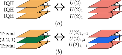
Figure 1: A schematic of our construction of LG theories for the (a) $U(2)_{3}$ and (b) $U(2)_{3,1}$ Fibonacci states. Here $\leftrightarrow$ denotes duality between the parent theories of ordinary Laughlin quasiparticles and dual theories of composite vortices coupled to $U(2)$ gauge fields. The non-Abelian state is obtained by clustering of the dual composite vortices between the layers.

Near $M=0$, this theory has been proposed to satisfy a large number of boson-fermion dualities [33], which are relativistic generalizations of the familiar flux attachment duality that relates the IQH transition of fermions to the condensation of composite bosons [23]. These relate the free Dirac fermion theory on each layer to one of a Wilson-Fisher boson, $\phi_{n}$, coupled to a fluctuating $U(N)$ Chern-Simons (CS) gauge field, $a_{n}$, in the fundamental representation [35, 36, 37]. While a free Dirac fermion has a bosonic dual for any value of $N$, our interest will be in the case of $N=2$,

$$\tilde{\mathcal{L}}_{\mathrm{IQH}}= \sum_{n=1}^{3}\left[|D_{a}\phi_{n}|^{2}-r|\phi_{n}|^{2}-|\phi_{n}|^{4}\right]$$

$$+\sum_{n=1}^{3}\mathcal{L}_{\mathrm{CS}}[a_{n}]+A_{\mu}j_{\mathrm{top}}^{\mu}\,,$$ (2)

$$\mathcal{L}_{\mathrm{CS}}[a_{n}]= \,\frac{1}{4\pi}\operatorname{Tr}\left[a_{n}da_{n}-\frac{2i}{3}(a_{n})^{3}\right]\,,$$ (3)

$$A_{\mu}j^{\mu}_{\mathrm{top}}= \,\frac{1}{2\pi}Ad\operatorname{Tr}[a_{1}-a_{2}+a_{3}]\,.$$ (4)

Here $-|\phi|^{4}$ denotes tuning such that the Wilson-Fisher fixed point occurs at $r=0$, and traces are over color (i.e. $U(2)$) indices. We have also selected the BF terms in Eq. (4) such that the second layer has opposite EM charge from the other two. Because each layer is decoupled from one another, we may freely determine the signs in Eq. (4) because the partition function has a charge conjugation symmetry.

The fact that the theory in Eq. (A composite particle construction of the Fibonacci fractional quantum Hall state) has the same phase diagram as that of Eq. (1) follows from the so-called level-rank duality of topological quantum field theories (TQFTs) [38, 39, 40, 35], which is an equivalence between $U(N)_{k}$ and $SU(k)_{-N}$ CS theories, where the subscript is the CS level. In particular, one can set $k=1$, leading to a duality between a trivial (i.e. IQH) theory and a $U(N)_{1}$ CS theory,

$$\mathcal{L}_{\mathrm{CS}}[b]+\frac{1}{2\pi}Ad\operatorname{Tr}[b] \longleftrightarrow-\frac{N}{4\pi}AdA\,,$$ (5)

where $b$ is a $U(N)$ gauge field, and we have suppressed gravitational Chern-Simons terms.

Using level-rank duality, we can check the phase diagram of Eq. (A composite particle construction of the Fibonacci fractional quantum Hall state): for $\operatorname{sgn}(r)>0$, the $\phi$ bosons are gapped, leading to a $U(2)_{1}$ theory on each layer, which describes a trilayer of $\nu=2$ IQH states by Eq. (5). Similarly, for $r<0$ the bosons condense, breaking the gauge group down to $U(1)$ on each layer. Integrating out the remaining $U(1)$ gauge fields leads to the desired trilayer $\nu=1$ response. The equivalence of the phase diagrams of the theories in Eqs. (1) and (A composite particle construction of the Fibonacci fractional quantum Hall state) has led to the conjecture that the critical points at $r=M=0$ are identical. Below we will assume this to be the case, our confidence bolstered by the large-$N,k$ derivations of Refs. [32, 31] and the Euclidean lattice derivation of Ref. [36].

Landau-Ginzburg theory. To target the Fibonacci phase, we first identify a CS TQFT representation of the state. It was recently shown [41] that one such representation is

$$U(2)_{3,1} =\frac{SU(2)_{3}\times U(1)_{2}}{\mathbb{Z}_{2}}.$$ (6)

This is a $U(2)$ CS gauge theory where the Abelian and non-Abelian parts of the gauge field have different CS levels. The quotient by $\mathbb{Z}_{2}$ simply enforces that these two components are part of the same $U(2)$ gauge field . The Lagrangian for this theory is written as

$$\mathcal{L}_{\mathrm{Fib}} =3\,\mathcal{L}_{\mathrm{CS}}[a]-\frac{1}{4\pi}\operatorname{Tr}[a]\,d\operatorname{Tr}[a]+\frac{1}{2\pi}Ad\operatorname{Tr}[a]\,,$$ (7)

where $a$ is again a $U(2)$ gauge field. One can check that this theory has a single nontrivial anyon, besides the vacuum, which transforms in the spin-1 representation of $U(2)$, satisfies the Fibonacci fusion rule, $\tau\times\tau=1+\tau$, and has topological spin $h_{\tau}=2/5$ [42]. We also comment that this theory is known to be dual to a $(G_{2})_{1}$ TQFT, where $G_{2}$ is the smallest exceptional simple Lie group [43, 16, 41].

To access the $U(2)_{3,1}$ state, we start by introducing inter-layer clustering to the composite vortex theory, Eq. (A composite particle construction of the Fibonacci fractional quantum Hall state), via coupling to a scalar field, $\Sigma_{nm}$,

$$\mathcal{L}_{\mathrm{cluster}} =-\sum_{n,m}\phi^{\dagger}_{m}\Sigma_{mn}\phi_{n}-V[\Sigma]\,.$$ (8)

Under gauge transformations, $\Sigma_{nm}\mapsto U_{m}\Sigma_{mn}U^{\dagger}_{n}$, where $U_{n}$ is a $U(2)$ gauge transformation on layer $n$. It can be understood as a Hubbard-Stratonovich field associated with the order parameter, $\phi^{\dagger}_{m}\phi_{n}$. We choose the potential $V[\Sigma]$ such that

$$\langle\Sigma_{mn}\rangle =M_{mn}\,\mathbf{1}_{2}\,,M_{mn}\neq 0\,,\,M_{nn}>0\,,\det M>0\,,$$ (9)

where $\mathbf{1}_{2}$ is the $2\times 2$ identity matrix in color space and $M_{mn}$ is a constant Hermitian matrix. In the resulting ground state, the $\phi_{n}$ fields are individually gapped, while the clustering order parameter, $\phi^{\dagger}_{m}\phi_{n}$ is condensed.

Because Eq. (9) is invariant under gauge transformations where $U_{1}=U_{2}=U_{3}$, the gauge group is broken as $U(2)\times U(2)\times U(2)\rightarrow U(2)$, Higgsing gauge field configurations except for those with $a_{1}=a_{2}=a_{3}\equiv a$. As a result, the CS terms for each of the $a_{n}$ gauge fields add, leading to a $U(2)_{3}$ theory,

$$\mathcal{L}_{U(3)_{3}}[a,A]=3\,\mathcal{L}_{\mathrm{CS}}[a]+\frac{1}{2\pi}Ad\operatorname{Tr}[a]\,.$$ (10)

Computing the Hall response by integrating out $\operatorname{Tr}[a]=\operatorname{Tr}[\tilde{a}\mathbf{1}_{2}]=2\tilde{a}$, one finds that the total filling fraction is now $\nu=2/3$, rather than $\nu=6$. The change in the filling fraction is related to our choice of charge assignments in Eq. (4), which results in the unit coefficient of the BF term in Eq. (10). While in the decoupled trilayer theory this choice of signs was immaterial, upon clustering the EM charge densities on each layer, $\rho_{n}=\varepsilon_{ij}\partial^{i}\operatorname{Tr}[a_{n}^{j}]/2\pi$, $i,j=x,y$, are pinned as $\rho_{1}=\rho_{3}=-\rho_{2}$, thereby breaking the discrete symmetry exchanging the layers and altering the filling fraction. The resulting minimal EM charge will prove crucial to obtaining the Fibonacci state.

The Fibonacci state, Eq. (7), is a descendant of the $U(2)_{3}$ state at $\nu=2/3$. To see this, we attach a single unit of flux to the “electrons,” the charges which couple to the background EM vector potential, $A_{\mu}$, and are understood to be the vortices of $\operatorname{Tr}[a]$ in the variables of Eq. (10). Since in our starting theory, Eq. (1), the EM charges are fermions, flux attachment shifts their statistics and renders the fundamental EM charges bosonic. Explicitly, introducing an Abelian statistical gauge field, $b$, we have

$$\mathcal{L} =\mathcal{L}_{U(3)_{3}}[a,b]+\frac{1}{4\pi}bdb+\frac{1}{2\pi}bdA+\frac{1}{4\pi}AdA\,.$$ (11)

Integrating out $b$, one immediately finds the Lagrangian in Eq. (7), which displays a $\nu=2$ Hall response. We have therefore found, using a combination of flux attachment and inter-layer clustering, a Fibonacci state of bosons at $\nu=2$.

The flux attachment transformation in Eq. (11) transmutes the original electric charges, which are fermions, to bosons, but it also mixes the three layers of the parent model, Eq. (1). A more physically transparent approach, which also leads to a Fibonacci state at $\nu=2$, proceeds by first attaching a positive flux to each electron on the first and third layers of the theory in Eq. (1) while attaching a negative flux to each electron on the second layer, explicitly breaking the layer exchange symmetry outright and leading to the parent theory depicted in Fig. 1(b). On the first and third layers, this results in theories of electrically charged Wilson-Fisher bosons on top of a $\nu=-2$ IQH state. On the second layer, however, this leads to Wilson-Fisher bosons coupled to the Halperin $(2,2,1)$ CS gauge theory at filling $\nu=+2/3$. One can show that clustering of composite vortices starting from this trilayer state leads to a Fibonacci FQH state [42]. We note that the Halperin $(2,2,1)$ state has appeared as a parent state for the Fibonacci order in related constructions [17, 44].

Using this bosonic parent description of Fig. 1(b), the final Landau-Ginzburg theory of the Fibonacci state can be expressed in terms of the clustering order parameter, $\Sigma$, after integrating out the composite vortices, $\phi$, and the auxiliary gauge fields associated with flux attachment,

$$\mathcal{L}= \sum_{m,n}\operatorname{Tr}\left[|\partial\Sigma_{mn}-ia_{m}\Sigma_{mn}+i\Sigma_{mn}a_{n}|^{2}\right]+\sum_{n}\mathcal{L}_{\mathrm{CS}}[a_{n}]$$

$$+\sum_{n}(-1)^{n}\left(\frac{1}{4\pi}\operatorname{Tr}[a_{n}]d\operatorname{Tr}[a_{n}]+\frac{1}{2\pi}Ad\operatorname{Tr}[a_{n}]\right)$$

$$-V_{r}[\Sigma]\,.$$ (12)

where the first term is a kinetic term generated by quantum corrections due to integrating out $\phi$, and $V_{r}$ is the renormalized potential for $\Sigma$. The trace is again over color indices. The phase diagram can be understood as in Fig. 2. For $\langle\Sigma\rangle=0$, the theory consists of three decoupled layers: two IQH insulators and a single Halperin $(2,2,1)$ layer. For $\langle\Sigma\rangle=M\neq 0$, the theory finds itself in a phase with Fibonacci topological order.

Furthermore, one can identify the Fibonacci anyons with gapped degrees of freedom in the Landau-Ginzburg theory; namely, the excitations of the adjoint bilinear of composite vortices, $\phi^{\dagger}t^{a}\phi$, where $t^{a}$ are the generators of $SU(2)\subset U(2)$. This can be observed from the fact that this operator transforms in the spin-1 representation of the gauge group and has vanishing electric charge, both properties of the Fibonacci anyon. Note that while the $\phi$ fields possess a layer index, in the Fibonacci state this does not lead to any unwanted degeneracy due to the condensation of $\langle\phi^{\dagger}_{m}\phi_{n}\rangle$, and so there is only one Fibonacci anyon.

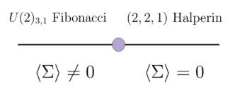
Figure 2: Phase diagram in terms of the clustering order parameter, $\Sigma$. The ordered state, $\langle\Sigma_{mn}\rangle=M_{mn}\mathbf{1}_{2}$, corresponds to the bosonic Fibonacci FQH state at filling $\nu=2$. The disordered phase, $\langle\Sigma_{mn}\rangle=0$, is a decoupled trilayer with the topological order of the Halperin $(2,2,1)$ state at total filling $\nu=-4+2/3=-10/3$.

Fibonacci wave function. Having developed an effective field theory that provides a concrete dynamical mechanism for how the Fibonacci state may be realized in a bosonic system at $\nu=2$, we now seek to develop an ideal wave function, which until now has also proven elusive. Ideal wave functions encode information about the clustering properties of electrons in non-Abelian states and can be compared with numerically obtained ground states in order to identify the topological order realized in realistic Hamiltonians. Remarkably, the wave function we will obtain displays a number of physical features that parallel the above effective field theory construction.

To obtain a wave function, we employ the standard conformal field theory (CFT) approach, in which the wave function is constructed in terms of correlation functions of the edge $(G_{2})_{1}\cong U(2)_{3,1}$ Wess-Zumino-Witten (WZW) CFT, $\Psi(\{z_{i}^{\sigma}\})=\langle\prod_{i=1}^{N}\Psi_{\sigma}(z_{i}^{\sigma})\rangle$ [2]. Here, $z_{i}^{\sigma}=x_{i}^{\sigma}+iy_{i}^{\sigma}$ are the complex coordinates of the electrons, $\sigma=1,\dots,n_{f}$ a type of “flavor” index, $n_{f}N$ is the number of electrons, and $\Psi_{\sigma}(z_{i})$ are operators in the CFT. Physically, $\Psi_{\sigma}(z)$ represents an electron operator and can in general be written as the product $\Psi_{\sigma}(z)=\psi_{\sigma}(z)e^{i\varphi(z)/\sqrt{\nu}}$, where $\nu$ is the filling fraction and $\varphi$ is a compact boson. The $\psi_{\sigma}(z)$ operators are electrically neutral. From Eq. (6), we observe that for the case at hand the $\psi_{\sigma}$’s are operators in the $SU(2)_{3}$ CFT, and $e^{i\varphi/\sqrt{\nu}}$, with $\nu=2$, is an operator in the $U(1)_{2}$ CFT.

The first step in constructing a wave function is therefore to determine the electron operators, $\Psi_{\sigma}$. We claim that the appropriate choice of electron operators is

$$\Psi_{\uparrow}\equiv\psi_{2}e^{i\phi/\sqrt{6}+i\varphi/\sqrt{2}},\quad\Psi_{\downarrow}\equiv\psi_{1}e^{-i\phi/\sqrt{6}+i\varphi/\sqrt{2}}.$$ (13)

Here we have made use of the fact that operators in the $SU(2)_{3}$ CFT can be expressed as products of vertex operators of another compact boson, $\phi$, and so-called $\mathbb{Z}_{3}$ parafermions [45], $\psi_{1}$ and $\psi_{2}$, which satisfy the operator product expansions (OPEs),

$$\psi_{1}(z)\psi_{1}(z^{\prime}) \sim(z-z^{\prime})^{-2/3}\psi_{2}(z^{\prime})+\dots\,\text{(likewise for }1\leftrightarrow 2)$$

$$\psi_{1}(z)\psi_{2}(z^{\prime}) \sim(z-z^{\prime})^{-4/3}+\dots\,.$$ (14)

The choice of the two electron operators (labeled by “spin” $\uparrow/\downarrow$) in Eq. (13) is motivated by the effective field theory construction discussed above. Indeed, the $(2,2,1)$ Halperin state involved in the parent state in Fig. 1(b) has two species of vortices satisfying a $\mathbb{Z}_{2}$ exchange symmetry and is commonly understood as a bilayer state; the remaining two layers in Fig. 1(b) are topologically trivial. We therefore anticipate that the Fibonacci wave function “knows” about this exchange symmetry and choose electron operators as such.

More formally, the need for two electron species arises from the fact that the electron operators must correspond to generators of the $(G_{2})_{1}$ current algebra, all of which represent local excitations. These can be labeled by the twelve roots of $G_{2}$, of which two are linearly independent. This suggests that we should have two distinct electron operators, as is the case for other FQH wave functions based on rank-two Lie algebras [46, 47, 48]. Following Refs. [46, 47], we require that our choice of electron operators is such that they have the same electric charge and opposite $SU(2)$ spin. The first requirement is satisfied via the two $e^{i\varphi/\sqrt{2}}$ factors; the second by the fact that their $SU(2)_{3}$ factors are conjugate to one another [42].

The Fibonacci wave function can thus be written as a $2N$-point correlation function of the $\Psi_{\uparrow/\downarrow}$ operators. The correlators of the vertex operators can be explicitly evaluated, and so we obtain (up to an overall Gaussian factor),

$$\begin{split}\Psi(\{z_{i},w_{i}\})&=\langle\prod_{i=1}^{N}\psi_{2}(z_{i})\psi_{1}(w_{i})\rangle\prod_{i,j}(z_{i}-w_{i})^{1/3}\\ &\qquad\times\prod_{i<j}(z_{i}-z_{j})^{2/3}\prod_{i<j}(w_{i}-w_{j})^{2/3},\end{split}$$ (15)

where $z_{i}$ ($w_{i}$) labels the position of the up (down) “spin.” This formal expression encodes key properties of the Fibonacci state. Indeed, the highest power of $z_{1}$ appearing in the factors multiplying the parafermion correlator is $2N(1/2)$, yielding a filling fraction of $\nu=2$, consistent with our field theory construction. Additionally, one can use Eq. (14) to see that the wave function satisfies the same three-body clustering as the $\mathbb{Z}_{3}$ RR wave function [14] separately in each of the $z_{i}$ and $w_{i}$ coordinates, dovetailing with our description in terms of clustering of composite vortices. These parallels between our proposed wave function and our dynamical construction above are encouraging, giving us confidence that Eq. (15) does indeed describe the Fibonacci state.

By using Eq. (14) to point-split $\psi_{2}$ into a product of $\psi_{1}$’s, one can explicitly evaluate the above parafermion correlator to express Eq. (15) as

$$\Psi(\{z_{i},w_{i}\}) =\frac{\Psi_{RR}^{k=3}(\{z_{i},z_{i},w_{i}\})}{\prod_{i<j}(z_{i}-z_{j})^{2}\prod_{i,j}(z_{i}-w_{j})},$$ (16)

where $\Psi_{RR}^{k=3}(\{z_{i},z_{i},w_{i}\})$ is the bosonic $\nu=3/2$ RR wave function for $3N$ particles, with the coordinates of $N$ pairs of particles set equal to one another [42]. The apparent asymmetry in $z_{i}$ and $w_{i}$ is an artifact of choosing to point-split the $\psi_{2}$’s. A manifestly symmetric wave function can be obtained via symmetric combination with the wave function obtained by point-splitting the $\psi_{1}$’s. Note that while the wave function exhibits a simple pole as we bring $z_{i}\to w_{i}$, we expect that this short-distance singularity can be regularized without altering the topological properties of the wave function.

Discussion. In this article, we have presented both a field-theoretic construction of the bosonic Fibonacci state at $\nu=2$ based on non-Abelian composite particle dualities, as well as an explicit wave function for this state. Our construction involves a parent trilayer system, in which the Fibonacci state is realized via clustering of dual “composite vortices” coupled to fluctuating $U(2)$ gauge fields. Leveraging this construction, we obtain a wave function for the Fibonacci state sharing many of the physical properties of our field-theoretic construction. Our approach can therefore be used to generate many other exotic states in need of a microscopic construction, as well as to motivate their wave functions.

Unlike other non-Abelian states, short-distance constructions of the Fibonacci state, particularly in isotropic systems, have proven elusive. The fact that our construction is based on a parent state involving fairly germane bosonic FQH phases suggests that a Fibonacci state may be realizable in the laboratory. Furthermore, the fact that the wave function for the $\nu=2$ bosonic Fibonacci state is manifestly holomorphic clearly suggests that it should be the ground state of a local Hamiltonian projected into a Landau level, and we hope that our wave function will motivate numerical studies in this direction. Additionally, going forward, it will be of interest to construct a transparent fermionic analogue of the bosonic Fibonacci state presented here, which would reproduce the state found in Ref. [29].

One may ask whether a different choice of electron operators would have yielded an equally reasonable candidate wave function. In particular, the $\Psi_{\uparrow/\downarrow}$ operators we defined are part of an $SU(2)$ quartet. For example, the wave function one obtains by choosing the other pair of operators within this quartet as the electrons describes the Abelian Halperin $(2,2,-1)$ state. While it is possible to obtain this state from our parent trilayer theory, it would be interesting to explore how different choices of electron operator in the CFT language may represent different parts of the bulk phase diagram.

Acknowledgements. We thank J. Alicea, B. Han, S. Raghu, S. Simon, T. Senthil, M. Stone, J.C.Y. Teo, and C. Xu for discussions and comments on the manuscript. This work was supported in part by the Gordon and Betty Moore Foundation EPiQS Initiative through Grant No. GBMF8684 at the Massachusetts Institute of Technology (HG), by the Natural Sciences and Engineering Research Council of Canada (NSERC) [funding reference number 6799-516762-2018] (RS), and by the US National Science Foundation grant DMR 1725401 at the University of Illinois (EF).

Appendix

.1 Chern-Simons conventions

Here we lay out our conventions for non-Abelian Chern-Simons gauge theories. We define $U(N)$ gauge fields $a_{\mu}=a^{b}_{\mu}t^{b}$, where $t^{b}$ are the (Hermitian) generators of the Lie algebra of $U(N)$, which satisfy $[t^{a},t^{b}]=if^{abc}t^{c}$, where $f^{abc}$ are the structure constants of $U(N)$. The generators are normalized so that $\operatorname{Tr}[t^{b}t^{c}]=\frac{1}{2}\delta^{bc}$. The trace of $a$ is a $U(1)$ gauge field, which we require to satisfy the Dirac quantization condition,

$$\int_{\Sigma}\frac{d\operatorname{Tr}[a]}{2\pi}=n\in\mathbb{Z}\,.$$ (17)

where $\Sigma\subset X$ is an oriented 2-cycle in spacetime, which we denote $X$. If $a_{\mu}$ couples to fermions, then it is a spin_c connection, and it satisfies a modified flux quantization condition

$$\int_{\Sigma}\frac{d\operatorname{Tr}[a]}{2\pi}=\int_{\Sigma}\frac{w_{2}}{2}+n\,,\,n\in\mathbb{Z}\,,$$ (18)

where $w_{2}$ is the second Stiefel-Whitney class of $X$. In general, the Chern-Simons levels for the $SU(N)$ and $U(1)$ components of $a$ can be different. We therefore adopt the standard notation [33],

$$U(N)_{k,k^{\prime}}=\frac{SU(N)_{k}\times U(1)_{Nk^{\prime}}}{\mathbb{Z}_{N}}\,.$$ (19)

By taking the quotient with $\mathbb{Z}_{N}$, we are restricting the difference of the $SU(N)$ and $U(1)$ levels to be an integer multiple of $N$,

$$k^{\prime}=k+nN\,,n\in\mathbb{Z}\,.$$ (20)

This enables us to glue the $U(1)$ and $SU(N)$ gauge fields together to form a gauge invariant theory of a single $U(N)$ gauge field $a=a_{SU(N)}+\tilde{a}\,\mathbf{1}$, with $\operatorname{Tr}[a]=N\tilde{a}$ having quantized fluxes as in Eq. (17). The Lagrangian for the $U(N)_{k,k^{\prime}}$ theory can be written as

$$\mathcal{L}_{U(N)_{k,k^{\prime}}} =\frac{k}{4\pi}\operatorname{Tr}[ada-\frac{2i}{3}a^{3}]+\frac{k^{\prime}-k}{4\pi N}\operatorname{Tr}[a]d\operatorname{Tr}[a]$$ (21)

$$=\frac{k}{4\pi}\operatorname{Tr}\left[a_{SU(N)}da_{SU(N)}-\frac{2i}{3}a_{SU(N)}^{3}\right]+\frac{Nk^{\prime}}{4\pi}\tilde{a}d\tilde{a}\,.$$ (22)

For the case $k=k^{\prime}$, we simply refer to the theory as $U(N)_{k}$.

Throughout this paper, we implicitly regulate non-Abelian (Abelian) gauge theories using Yang-Mills (Maxwell) terms, as opposed to dimensional regularization [49, 50]. In Yang-Mills regularization, there is a one-loop exact shift of the $SU(N)$ level, $k\rightarrow k+\operatorname{sgn}(k)N$, that does not appear in dimensional regularization. Consequently, to describe the same theory in dimensional regularization, one must start with a $SU(N)$ level $k_{\mathrm{DR}}=k+\operatorname{sgn}(k)N$. The dualities discussed in this paper therefore would take a somewhat different form in dimensional regularization.

.2 Derivation of the bosonic parent state from intra-layer flux attachment

Here we describe the intra-layer flux attachment procedure described in the main text, which yields the bosonic parent state depicted in Fig. 1(b). We start again with a trilayer of free Dirac fermions near a $\nu=2\rightarrow 1$ plateau transition,

$$\mathcal{L}_{\mathrm{IQH}} =\sum_{n=1}^{3}\left[\bar{\Psi}_{n}(i\not{D}_{A}-M)\Psi_{n}-\frac{3}{2}\frac{1}{4\pi}AdA\right]\,.$$ (23)

This theory is dual to a trilayer of Wilson-Fisher composite bosons, $\Phi_{n}$, coupled to fluctuating CS gauge fields, $\alpha_{n}$, [51, 52],

$$\mathcal{L}_{\mathrm{IQH}}[A]\leftrightarrow\sum_{n}{\mathcal{L}}^{\Phi}_{n}[\Phi_{n},\alpha_{n},A] =\sum_{n}\left[|D_{\alpha_{n}}\Phi_{n}|^{2}-r|\Phi_{n}|^{2}-|\Phi_{n}|^{4}+\frac{1}{4\pi}\alpha_{n}d\alpha_{n}+\frac{1}{2\pi}Ad\alpha_{n}-\frac{1}{4\pi}AdA\right]\,,$$ (24)

where $-|\Phi|^{4}$ again denotes tuning such that the theory is at its Wilson-Fisher fixed point when $r=0$, and the phase diagrams of the two theories match if $\operatorname{sgn}(r)=-\operatorname{sgn}(M)$.

We now attach a positive flux to the electric charges on layers $n=1$ and $3$ and a negative flux to those on layer $n=2$. This is implemented in a manifestly gauge invariant way by the following transformation on each layer’s Lagrangian [53, 54],

$$\mathcal{L}^{\Phi}_{n}[\Phi_{n},\alpha_{n},A]\rightarrow\mathcal{L}^{\Phi}_{n}[\Phi_{n},\alpha_{n},\gamma_{n}]+\frac{1}{2\pi}\gamma_{n}d\beta_{n}+\frac{(-1)^{n}}{4\pi}\beta_{n}d\beta_{n}+\frac{1}{2\pi}Ad\beta_{n},$$ (25)

where $\beta_{n},\gamma_{n}$ are new fluctuating $U(1)$ gauge fields. One can easily check that the electric charges in the gapped phases of this theory have had their statistics shifted by $\pm\pi$. Because the equation of motion for $\gamma_{n}$ is

$$d(\alpha_{n}+\beta_{n})=d\gamma_{n}\,,$$ (26)

$\gamma_{n}$ may be integrated out while preserving flux quantization. The resulting Lagrangian on each layer is

$$\mathcal{L}^{\Phi}_{n}\equiv|D_{\alpha_{n}}\Phi_{n}|^{2}-r|\Phi_{n}|^{2}-|\Phi_{n}|^{4}+\frac{2}{4\pi}\alpha_{n}d\alpha_{n}+\frac{1}{4\pi}\left[1+(-1)^{n}\right]\frac{1}{4\pi}\beta_{n}d\beta_{n}+\frac{1}{2\pi}\alpha_{n}d\beta_{n}+\frac{1}{2\pi}Ad\beta_{n}\,,$$ (27)

where we have redefined $\mathcal{L}^{\Phi}_{n}$ to minimize the number of labels in use. On layers $n=1,3$, the CS term for $\beta_{n}$ vanishes. Integrating it out therefore Higgses $\alpha_{n}$ (in other words, sets $d\alpha_{n}=dA$), leaving a topologically trivial theory near a superconductor-insulator transition. On layer $n=2$, however, the CS term for $\beta_{n}$ has level 2, meaning that the gauge theory is topologically nontrivial and has the $K$-matrix of the Halperin (2,2,1) state. Explicitly, renaming $\alpha_{2}\equiv\alpha,\beta_{2}\equiv\beta$,

$$\mathcal{L}^{\Phi}_{p} =|D_{A}\Phi_{p}|^{2}-r|\Phi_{p}|^{2}-|\Phi_{p}|^{4}+\frac{2}{4\pi}AdA\,,\,p=1,3\,;$$ (28)

$$\mathcal{L}^{\Phi}_{2} =|D_{\alpha}\Phi_{2}|^{2}-r|\Phi_{2}|^{2}-|\Phi_{2}|^{4}+\frac{2}{4\pi}\alpha d\alpha+\frac{2}{4\pi}\beta d\beta+\frac{1}{2\pi}\alpha d\beta+\frac{1}{2\pi}\beta dA\,.$$ (29)

The trilayer theory, $\sum_{n}\tilde{\mathcal{L}}^{\Phi}_{n}$, is the theory depicted in Fig. 1(b).

We now check that these theories are dual to theories of composite vortices, which on clustering yield the Fibonacci state. Applying the duality used in Eq. (A composite particle construction of the Fibonacci fractional quantum Hall state) of the main text along with the transformation flux attachment transformation in Eq. (25), the dual theories of composite vortices are

$$\tilde{\mathcal{L}}^{\phi}_{n}\leftrightarrow\tilde{\mathcal{L}}_{p}^{\phi}=\, |D_{a}\phi_{p}|^{2}-\tilde{r}|\phi_{n}|^{2}-|\phi_{n}|^{4}+\frac{1}{4\pi}\operatorname{Tr}\left[a_{n}da_{n}-\frac{2i}{3}a^{3}_{n}\right]$$

$$+\frac{1}{2\pi}\gamma_{n}d\operatorname{Tr}[a_{n}]+\frac{1}{2\pi}\gamma_{n}d\beta_{n}+\frac{(-1)^{n}}{4\pi}\beta_{n}d\beta_{n}+\frac{1}{2\pi}Ad\beta_{n}\,,$$ (30)

where again $a_{n}$ are $U(2)$ gauge fields. In this case, both $\gamma_{n}$ and $\beta_{n}$ can be safely integrated out without running afoul of flux quantization: integrating out $\gamma_{n}$ implements a constraint on (i.e. Higgses) $\beta_{n}$, $d\beta_{n}=-d\operatorname{Tr}[a_{n}]$. The resulting theories involve $U(2)_{1,-1}$ gauge theories on layers $n=1,3$, which is topologically trivial [35], and a $U(2)_{1,3}$ theory on the $n=2$ layer,

$$\tilde{\mathcal{L}}^{\phi}_{n}=|D_{a}\phi_{p}|^{2}-\tilde{r}|\phi_{n}|^{2}-|\phi_{n}|^{4}+\frac{1}{4\pi}\operatorname{Tr}\left[a_{n}da_{n}-\frac{2i}{3}a^{3}_{n}\right]+(-1)^{n}\left[\frac{1}{4\pi}\operatorname{Tr}[a_{n}]d\operatorname{Tr}[a_{n}]+\frac{1}{2\pi}Ad\operatorname{Tr}[a_{n}]\right]\,.$$ (31)

As in the discussion in the main text, we are free to invoke charge conjugation symmetry to flip the sign of the BF term on layer $n=2$ relative to those on layers $1,3$. From here, it is straightforward to see that a nonzero expectation value for the clustering order parameter, $\langle\Sigma_{mn}\rangle=\langle\phi^{\dagger}_{m}\phi_{n}\rangle\neq 0$, sets $a_{1}=a_{2}=a_{3}\equiv a$ and produces the Fibonacci $U(2)_{3,1}$ TQFT,

$$\mathcal{L}_{\mathrm{Fib}} =\frac{3}{4\pi}\operatorname{Tr}\left[a_{n}da_{n}-\frac{2i}{3}a^{3}_{n}\right]-\frac{1}{4\pi}\operatorname{Tr}[a]\,d\operatorname{Tr}[a]+\frac{1}{2\pi}Ad\operatorname{Tr}[a]\,.$$ (32)

Integrating out the $\phi_{n}$ fields but leaving the Fibonacci order parameter thus leads to the final Landau-Ginzburg theory obtained in the main text,

$$\mathcal{L}= \sum_{m,n}\operatorname{Tr}\left[|\partial\Sigma_{mn}-ia_{m}\Sigma_{mn}+i\Sigma_{mn}a_{n}|^{2}\right]-V_{r}[\Sigma]$$

$$+\sum_{n}\left[\mathcal{L}_{\mathrm{CS}}[a_{n}]+(-1)^{n}\left(\frac{1}{4\pi}\operatorname{Tr}[a_{n}]d\operatorname{Tr}[a_{n}]+\frac{1}{2\pi}Ad\operatorname{Tr}[a_{n}]\right)\right]\,.$$ (33)

.3 Representation of the Fibonacci order in terms of $U(2)_{3,1}$

In this section, we demonstrate explicitly that $U(2)_{3,1}=[SU(2)_{3}\times U(1)_{2}]/\mathbb{Z}_{2}$ possesses the same anyon content as that of $(G_{2})_{1}$, namely, just the Fibonacci anyon. There are multiple ways to describe the process of enforcing the $\mathbb{Z}_{2}$ quotient in the definition of $U(2)_{3,1}$. From the perspective of the anyon content of the theories, this quotient amounts to condensing [55] a bosonic anyon in the $SU(2)_{3}\times U(1)_{2}$ product theory with $\mathbb{Z}_{2}$ fusion rules and either $0$ or $\pi$ braiding statistics with all other anyons. The condensed anyon is then identified as a local quasiparticle, and so all anyons with which it braids nontrivially are projected out. In order to identify the anyon to be condensed, let us remind ourselves of the anyon content of the $SU(2)_{3}$ and $U(1)_{2}$ factors:

$$U(1)_{2} :\qquad 1,\,s$$ (34)

$$SU(2)_{3} :\qquad[0],\,[1/2],\,[1],\,[3/2].$$ (35)

Here, $s$ is the semion, which has topological spin $h_{s}=1/4$ and satisfies the fusion rule $s\times s=1$. We have labelled the anyons of $SU(2)_{3}$ by the representation of $SU(2)$ under which they transform. They are all self-dual, satisfying the fusion rules

$$[0]\times[0] =[0]$$ (36)

$$[1/2]\times[1/2] =[0]+[1]$$ (37)

$$[1]\times[1] =[0]+[1]$$ (38)

$$[3/2]\times[3/2] =[0].$$ (39)

From this, we see that $[1]$, which has spin $h_{[1]}=2/5$, is the Fibonacci. The only Abelian anyon is $[3/2]$, which has spin $h_{[3/2]}=3/4$, trivial braiding with $[1]$, and non-trivial braiding with $[1/2]$. We immediately see that, in the product theory, $[3/2]s$ is an Abelian anyon with spin unity. On condensing this anyon, all anyons aside from the Fibonacci will become confined, yielding the desired $(G_{2})_{1}$ Fibonacci topological order.

.4 Constructing the Electron Operators

As stated in the main text, the electron operators used in constructing the Fibonacci wave function must be selected from the generators of the $(G_{2})_{1}$ current algebra. We present the technical details of this process here. The $(G_{2})_{1}$ current algebra has fourteen generators, twelve of which are labeled by the roots of $G_{2}$. In order to obtain explicit expressions for these operators, we make use of the duality between $(G_{2})_{1}$ and $U(2)_{3,1}=[SU(2)_{3}\times U(1)_{2}]/\mathbb{Z}_{2}$, which will allow us to write the generators in terms of operators in the $SU(2)_{3}$ and $U(1)_{2}$ conformal field theories (CFTs).

The $U(1)_{2}$ factor is described by a chiral boson, $\varphi$, with compactification radius $R=1$. It supports a single anyon, the semion, represented by the vertex operator

$$s(z)\equiv e^{i\varphi(z)/\sqrt{2}},$$ (40)

which has scaling dimension $\Delta_{s}=1/4$. The operators $s^{2}=e^{i\sqrt{2}\varphi}$ and $\bar{s}^{2}=e^{-i\sqrt{2}\varphi}$ generate the $U(1)_{2}$ chiral algebra, and so correspond to local excitations.

As for $SU(2)_{3}$, its primary fields, like the anyons in the corresponding TQFT, fall into four topological sectors labelled by the $SU(2)$ representation under which they transform: $[j]$, $j=0,1/2,1,3/2$. In order to write down explicit forms of these fields and the current operators, we make use of the fact that the operators of $SU(2)_{3}$ can be expressed in terms of products of operators in the $k=3$ parafermion and $U(1)_{6}$ CFTs, the former of which we will write as $\text{Parafermion}_{3}$. The $U(1)_{6}$ CFT is described by a chiral boson $\phi$ at radius $R=1$, with primary fields

$$a^{l}(z)\equiv e^{il\phi/\sqrt{6}},\quad l=0,\dots,5$$ (41)

These fields have scaling dimensions $\Delta_{l}=l^{2}/12$, from which we see that the field $a^{6}$ represents a local excitation. The primary fields of the $\text{Parafermion}_{3}$CFT and their scaling dimensions are given in Table 1 while their fusion rules are given in Table 2. The raising and lowering operators of the $SU(2)_{3}$ algebra are given by the operators,

$$\psi_{1}a^{2}=\psi_{1}e^{i\sqrt{2/3}\phi},\quad\psi_{1}^{\dagger}\bar{a}^{2}=\psi_{2}e^{-i\sqrt{2/3}\phi}.$$ (42)

	$1$	$\psi_{1}$	$\psi_{2}$	$\sigma_{1}$	$\sigma_{2}$	$\epsilon$
$\Delta$	0	$2/3$	$2/3$	$1/15$	$1/15$	$2/5$

Table 1: Scaling dimensions of the $\text{Parafermion}_{3}$primary fields.

$\times$	$\psi_{1}$	$\psi_{2}$	$\sigma_{1}$	$\sigma_{2}$	$\epsilon$
$\psi_{1}$	$\psi_{2}$
$\psi_{2}$	$1$	$\psi_{1}$
$\sigma_{1}$	$\epsilon$	$\sigma_{2}$	$\sigma_{2}+\psi_{1}$
$\sigma_{2}$	$\sigma_{1}$	$\epsilon$	$1+\epsilon$	$\sigma_{1}+\psi_{2}$
$\epsilon$	$\sigma_{2}$	$\sigma_{1}$	$\sigma_{1}+\psi_{2}$	$\sigma_{2}+\psi_{1}$	$1+\epsilon$

Table 2: Fusion rules of $\text{Parafermion}_{3}$.

Now, in order to obtain the $(G_{2})_{1}$ algebra from $SU(2)_{3}\times U(1)_{2}$, we must perform the $\mathbb{Z}_{2}$ quotient. As in the TQFT description, this corresponds to condensing operators in the

$$\left[\frac{3}{2}\right]s$$ (43)

topological sectors. In the language of CFT, this “condensation” means that the operators in these topological sectors will be identified as generators of the $[SU(2)_{3}\times U(1)_{2}]/\mathbb{Z}_{2}$ (equivalently, $(G_{2})_{1}$) CFT. Explicitly, the operators

$$\bar{a}^{3},\quad\psi_{1}\bar{a},\quad\psi_{2}a,\quad a^{3}$$ (44)

are all in the $[3/2]$ sector, and so are topologically equivalent. Indeed, each is related to the other by fusion with the $SU(2)_{3}$ generators, forming an $SU(2)_{3}$ quartet. Hence, performing the $\mathbb{Z}_{2}$ quotient means condensing the operators

$$\begin{split}\bar{a}^{3}s,\quad\psi_{1}\bar{a}s,\quad\psi_{2}as,\quad a^{3}s\\ \bar{a}^{3}\bar{s},\quad\psi_{1}\bar{a}\bar{s},\quad\psi_{2}a\bar{s},\quad a^{3}\bar{s}\end{split}$$ (45)

This set of operators, combined with the generators of $SU(2)_{3}$ and $U(1)_{2}$ constitute the twelve generators of $(G_{2})_{1}$ labelled by its roots [56].

Fig. 3 depicts the $G_{2}$ root system labeled by the corresponding current generators. One can check that vector addition of the roots matches up with fusion of the corresponding current operators. Note also that the generators naturally organize themselves in terms of their transformation properties under $SU(2)$ and $U(1)$. The vertical coordinate of the root corresponds to the $U(1)$ charge and the horizontal coordinate to the $SU(2)$ spin.

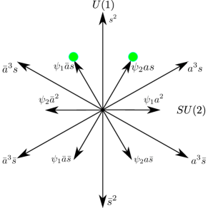
Figure 3: Root system of $G_{2}$ labelled by the corresponding $(G_{2})_{1}$ current generators. The green circles indicate the operators we identify as the electron operators.

It now remains to determine which generators we should identify as the physical electrons. In the spirit of Refs. [46, 47], we expect that we must choose two electron operators, by virtue of the fact that the root system is two-dimensional. The electrons should have the same positive charge, suggesting we should restrict ourselves to the upper half-plane of the root system. As described in the main text, we expect the Fibonacci wave function to describe a two-flavor system, and so the electron operators should have opposite $SU(2)$ spin. We thus claim that

$$\begin{split}\Psi_{\uparrow}&\equiv\psi_{2}as=\psi_{2}e^{i\phi/\sqrt{6}+i\varphi/\sqrt{2}},\\ \Psi_{\downarrow}&\equiv\psi_{1}\bar{a}s=\psi_{2}e^{-i\phi/\sqrt{6}+i\varphi/\sqrt{2}}\end{split}$$ (46)

are the appropriate electron operators.

We note that operators $\bar{a}^{3}s$ and $a^{3}s$ also satisfy our two criteria for charge and spin. In fact, $\Psi_{\uparrow}$ and $\Psi_{\downarrow}$ form an $SU(2)$ quartet with $\bar{a}^{3}s$ and $a^{3}s$ (as can be seen from Fig. 3), and so one may reasonably ask whether the latter two operators constitute equally valid choices for the electron operator. As it turns out, the wave function obtained from $\bar{a}^{3}s$ and $a^{3}s$ describes an Abelian state, as we demonstrate in the following section. This suggests, a posteriori, that $\Psi_{\uparrow/\downarrow}$ are the correct electron operators needed to obtain a wave function describing the non-Abelian Fibonacci state.

.5 Derivation of the Fibonacci Wave Function

In this section, we present a computation of the explicit form of the Fibonacci wave function provided in the main text. With the choice of electron operators given in Eq. (46), we can express the wave function as

$$\Psi(\{z_{i},w_{i}\})=\langle\prod_{i=1}^{N}\Psi_{\uparrow}(z_{i})\Psi_{\downarrow}(w_{i})O_{bg}\rangle=\langle\prod_{i=1}^{N}\psi_{2}as(z_{i})\psi_{1}\bar{a}s(w_{i})O_{bg}\rangle,$$ (47)

where $z_{i}$ and $w_{i}$ label the positions of the up and down spins (spin is used as a stand-in for some flavor index). Here $O_{bg}$ is a background charge operator that ensures the correlator of the $s$ fields is non-vanishing and yields the usual Gaussian factor on the plane [57]. Note that such an operator for the $a$ fields is not necessary, since there are an equal number of $a$ and $\bar{a}$ fields, ensuring their charge neutrality condition is satisfied. Physically, this is a consequence of the fact that it is the $U(1)_{2}$ sector and hence the $s$ fields which are charged under the external electromagnetic field. We thus obtain (dropping the usual overall Gaussian factor),

$$\Psi(\{z_{i},w_{i}\}) =\langle\prod_{i=1}^{N}\psi_{2}(z_{i})\psi_{1}(w_{i})\rangle\langle\prod_{i=1}^{N}e^{i\frac{1}{\sqrt{6}}\phi(z_{i})}e^{-i\frac{1}{\sqrt{6}}\phi(w_{i})}\rangle\langle\prod_{i=1}^{N}e^{i\frac{1}{\sqrt{2}}\varphi(z_{i})}e^{i\frac{1}{\sqrt{2}}\varphi(w_{i})}O_{bg}\rangle$$ (48)

$$=\langle\prod_{i=1}^{N}\psi_{2}(z_{i})\psi_{1}(w_{i})\rangle\prod_{i,j}(z_{i}-w_{i})^{1/3}\prod_{i<j}(z_{i}-z_{j})^{2/3}\prod_{i<j}(w_{i}-w_{j})^{2/3}.$$ (49)

In order to evaluate the remaining correlator, we can use the parafermion operator product expansions (OPEs),

$$\psi_{1}(z)\psi_{1}(z^{\prime}) \sim(z-z^{\prime})^{-2/3}\psi_{2}(z^{\prime})+\dots\,\text{(likewise for }1\leftrightarrow 2)$$

$$\psi_{1}(z)\psi_{2}(z^{\prime}) \sim(z-z^{\prime})^{-4/3}+\dots\,.$$ (50)

to effectively point-split the $\psi_{2}$ operators into products of $\psi_{1}$ operators:

$$\langle\prod_{i=1}^{N}\psi_{1}(z_{i}^{1})\psi_{1}(z_{i}^{2})\psi_{1}(w_{i})\rangle=\langle\prod_{i=1}^{N}(z_{i}^{1}-z_{i}^{2})^{-2/3}\psi_{2}(z_{i}^{2})\psi_{1}(w_{i})\rangle+\dots\,,$$ (51)

where, here and in the following, the limit $z_{i}^{1}\to z_{i}^{2}$ is taken implicitly. The ellipsis represent less singular terms in the $\psi_{1}\times\psi_{1}$ OPE which vanish in this limit, allowing us to isolate the desired parafermion correlator when we take $z_{i}^{1}=z_{i}^{2}\equiv z_{i}$ at the end of the computation.

Now, the correlator of $\psi_{1}$ fields is precisely given in terms of the Read-Rezayi (RR) wave functions:

$$\langle\prod_{i=1}^{N}\psi_{1}(z_{i}^{1})\psi_{1}(z_{i}^{2})\psi_{1}(w_{i})\rangle=\Psi_{RR}^{k=3}(\{z_{i}^{1},z_{i}^{2},w_{i}\})\Psi_{LJ}^{-2/3}(\{z_{1}^{1},z_{i}^{2},w_{i}\}).$$ (52)

Here, $\Psi_{RR}^{k=3}$ and $\Psi_{LJ}(\{z_{i}\})=\prod_{i<j}(z_{i}-z_{j})$ are the $\nu=3/2$ bosonic RR (taking $k=3$ and $M=0$ in the notation of Ref. [14]) and Landau-Jastrow wave functions, respectively. Hence,

$$\langle\prod_{i=1}^{N}\psi_{2}(z_{i}^{2})\psi_{1}(w_{i})\rangle+\ldots =\Psi_{RR}^{k=3}(\{z_{i}^{1},z_{i}^{2},w_{i}\})\Psi_{LJ}^{-2/3}(\{z_{1}^{1},z_{i}^{2},w_{i}\})\prod_{i=1}^{N}(z_{i}^{1}-z_{i}^{2})^{2/3}$$ (53)

$$\begin{split}&=\Psi_{RR}^{k=3}(\{z_{i}^{1},z_{i}^{2},w_{i}\})\prod_{i<j}(z_{i}^{1}-z_{j}^{1})^{-2/3}(z_{i}^{2}-z_{j}^{2})^{-2/3}(w_{i}-w_{j})^{-2/3}\\ &\qquad\qquad\times\prod_{i\neq j}(z_{i}^{1}-z_{j}^{2})^{-2/3}\prod_{i,j}(z_{i}^{1}-w_{j})^{-2/3}(z_{i}^{2}-w_{j})^{-2/3}.\end{split}$$ (54)

We can now safely set $z_{i}^{1}=z_{i}^{2}\equiv z_{i}$, in which case the terms contained in the ellipsis vanish identically. Combining terms and ignoring unimportant overall phase factors, we obtain

$$\Psi(\{z_{i},w_{i}\}) =\Psi_{RR}^{k=3}(\{z_{i},z_{i},w_{i}\})\prod_{i<j}(z_{i}-z_{j})^{-2}\prod_{i,j}(z_{i}-w_{j})^{-1}$$ (55)

as our Fibonacci wave function. Here, $\Psi_{RR}^{k=3}(\{z_{i},z_{i},w_{i}\})$ is the bosonic $\nu=3/2$ RR wave function for $3N$ particles, with the coordinates of $N$ pairs of these particles set equal to one another. As noted in the main text, the asymmetry in $z_{i}$ and $w_{i}$ is a consequence of having point-split the $\psi_{2}$ parafermions as opposed to the $\psi_{1}$ parafermions. Had we instead point-split the $\psi_{1}$ parafermions into products of $\psi_{2}$ parafermions, we would have obtained the above expression with $z_{i}$ and $w_{i}$ exchanged. Since the expressions obtained via these two different point-splitting procedures must necessarily be equal, we can write down the wave function in a manifestly symmetric way by taking their average:

$$\Psi(\{z_{i},w_{i}\}) =\frac{1}{2}\left(\frac{\Psi_{RR}^{k=3}(\{z_{i},z_{i},w_{i}\})}{\prod_{i<j}(z_{i}-z_{j})^{2}}+\frac{\Psi_{RR}^{k=3}(\{z_{i},w_{i},w_{i}\})}{\prod_{i<j}(w_{i}-w_{j})^{2}}\right)\prod_{i,j}(z_{i}-w_{j})^{-1}.$$ (56)

Finally, we return to the remark regarding the choice of electron operators made at the end of the preceding section. Had we instead attempted to construct a wave function using $\Psi_{\uparrow\uparrow}=a^{3}s$ and $\Psi_{\downarrow\downarrow}=\bar{a}^{3}s$ as the electron operators, we would have obtained

$$\tilde{\Psi}(\{z_{i},w_{i}\})=\langle\prod_{i=1}^{N}\Psi_{\uparrow\uparrow}(z_{i})\Psi_{\downarrow\downarrow}(w_{i})O_{bg}\rangle=\langle\prod_{i=1}^{N}e^{i\sqrt{\frac{3}{2}}\phi(z_{i})}e^{-i\sqrt{\frac{3}{2}}\phi(w_{i})}\rangle\langle\prod_{i=1}^{N}e^{i\frac{1}{\sqrt{2}}\varphi(z_{i})}e^{i\frac{1}{\sqrt{2}}\varphi(w_{i})}O_{bg}\rangle\,.$$ (57)

The correlators of vertex operators can be straightforwardly evaluated to obtain

$$\tilde{\Psi}(\{z_{i},w_{i}\})=\prod_{i<j}(z_{i}-z_{j})^{2}(w_{i}-w_{j})^{2}\prod_{i,j}(z_{i}-w_{j})^{-1},$$ (58)

which describes the Abelian Halperin $(2,2,-1)$ state, again at filling $\nu=2$. This gives us some confidence that $\Psi(\{z_{i},w_{i}\})$ correctly describes the Fibonacci state.

References

- Nayak et al. [2008] C. Nayak, S. H. Simon, A. Stern, M. Freedman, and S. Das Sarma, Non-Abelian anyons and topological quantum computation, Rev. Mod. Phys. 80, 1083 (2008).
- Moore and Read [1991] G. Moore and N. Read, Nonabelions in the fractional quantum hall effect, Nuclear Physics B 360, 362 (1991).
- Chamon et al. [1997] C. Chamon, D. E. Freed, S. A. Kivelson, S. L. Sondhi, and X. G. Wen, Two point-contact interferometer for quantum Hall systems, Phys. Rev. B 55, 2331 (1997).
- Fradkin et al. [1998] E. Fradkin, C. Nayak, A. Tsvelik, and F. Wilczek, A Chern-Simons effective field theory for the Pfaffian quantum Hall state, Nuclear Physics B 516, 704 (1998).
- Bonderson et al. [2006] P. Bonderson, A. Kitaev, and K. Shtengel, Detecting non-abelian statistics in the fractional quantum Hall state, Phys. Rev. Lett. 96, 016803 (2006).
- Stern and Halperin [2006] A. Stern and B. I. Halperin, Proposed Experiments to Probe the Non-Abelian Quantum Hall State, Phys. Rev. Lett. 96, 016802 (2006).
- Bishara et al. [2009] W. Bishara, P. Bonderson, C. Nayak, K. Shtengel, and J. K. Slingerland, Interferometric signature of non-Abelian anyons, Phys. Rev. B 80, 155303 (2009).
- Nakamura et al. [2020] J. Nakamura, S. Liang, G. C. Gardner, and M. J. Manfra, Direct observation of anyonic braiding statistics, Nature Physics 16, 931 (2020).
- Radu et al. [2008] I. P. Radu, J. B. Miller, C. M. Marcus, M. A. Kastner, L. N. Pfeiffer, and K. W. West, Quasi-Particle Properties from Tunneling in the v = 5/2 Fractional Quantum Hall State, Science 320, 899 (2008).
- Dolev et al. [2008] M. Dolev, M. Heiblum, V. Umansky, A. Stern, and D. Mahalu, Observation of a quarter of an electron charge at the quantum Hall state, Nature 452, 829 (2008).
- Willett et al. [2009] R. L. Willett, L. N. Pfeiffer, and K. W. West, Measurement of filling factor 5/2 quasiparticle interference with observation of charge e/4 and e/2 period oscillations, Proceedings of the National Academy of Sciences 106, 8853 (2009).
- Willett et al. [2013] R. L. Willett, C. Nayak, K. Shtengel, L. N. Pfeiffer, and K. W. West, Magnetic-Field-Tuned Aharonov-Bohm Oscillations and Evidence for Non-Abelian Anyons at , Phys. Rev. Lett. 111, 186401 (2013).
- Freedman et al. [2002] M. H. Freedman, M. Larsen, and Z. Wang, A Modular Functor Which is Universal for Quantum Computation, Communications in Mathematical Physics 227, 605 (2002).
- Read and Rezayi [1999] N. Read and E. Rezayi, Beyond paired quantum Hall states: Parafermions and incompressible states in the first excited Landau level, Phys. Rev. B 59, 8084 (1999).
- Pakrouski et al. [2016] K. Pakrouski, M. Troyer, Y.-L. Wu, S. Das Sarma, and M. R. Peterson, Enigmatic 12/5 fractional quantum Hall effect, Phys. Rev. B 94, 075108 (2016).
- Mong et al. [2017] R. S. K. Mong, M. P. Zaletel, F. Pollmann, and Z. Papić, Fibonacci anyons and charge density order in the 12/5 and 13/5 quantum Hall plateaus, Phys. Rev. B 95, 115136 (2017).
- Mong et al. [2014] R. S. K. Mong, D. J. Clarke, J. Alicea, N. H. Lindner, P. Fendley, C. Nayak, Y. Oreg, A. Stern, E. Berg, K. Shtengel, and M. P. A. Fisher, Universal Topological Quantum Computation from a Superconductor-Abelian Quantum Hall Heterostructure, Phys. Rev. X 4, 011036 (2014).
- Hu and Kane [2018] Y. Hu and C. L. Kane, Fibonacci Topological Superconductor, Phys. Rev. Lett. 120, 066801 (2018).
- Lopes et al. [2019] P. L. S. Lopes, V. L. Quito, B. Han, and J. C. Y. Teo, Non-Abelian twist to integer quantum Hall states, Phys. Rev. B 100, 085116 (2019).
- Teo and Kane [2014] J. C. Y. Teo and C. L. Kane, From Luttinger liquid to non-Abelian quantum Hall states, Phys. Rev. B 89, 085101 (2014).
- Fendley and Fradkin [2005] P. Fendley and E. Fradkin, Realizing non-abelian statistics in time-reversal-invariant systems, Phys. Rev. B 72, 024412 (2005).
- Jain [1989] J. K. Jain, Composite-fermion approach for the fractional quantum Hall effect, Phys. Rev. Lett. 63, 199 (1989).
- Zhang et al. [1989] S. C. Zhang, T. H. Hansson, and S. Kivelson, Effective-Field-Theory Model for the Fractional Quantum Hall Effect, Phys. Rev. Lett. 62, 82 (1989).
- López and Fradkin [1991] A. López and E. Fradkin, Fractional quantum Hall effect and Chern-Simons gauge theories, Phys. Rev. B 44, 5246 (1991).
- Read and Green [2000] N. Read and D. Green, Paired states of fermions in two dimensions with breaking of parity and time-reversal symmetries and the fractional quantum Hall effect, Phys. Rev. B 61, 10267 (2000).
- Fradkin et al. [1999] E. H. Fradkin, C. Nayak, and K. Schoutens, Landau-Ginzburg theories for nonAbelian quantum Hall states, Nucl. Phys. B546, 711 (1999), arXiv:cond-mat/9811005 [cond-mat] .
- Goldman et al. [2019] H. Goldman, R. Sohal, and E. Fradkin, Landau-Ginzburg theories of non-Abelian quantum Hall states from non-Abelian bosonization, Phys. Rev. B 100, 115111 (2019).
- Radicevic et al. [2016] D. Radicevic, D. Tong, and C. Turner, Non-Abelian 3d Bosonization and Quantum Hall States, JHEP 2016 (12), 067, 1608.04732 .
- Goldman et al. [2020] H. Goldman, R. Sohal, and E. Fradkin, Non-Abelian fermionization and the landscape of quantum Hall phases, Phys. Rev. B 102, 195151 (2020).
- Note [1] In Ref. [29], we already predicted a phase transition between a integer quantum Hall (IQH) state of fermions and a Fibonacci state at , but this transition involves very strongly interacting physics, and its physical interpretation remains mysterious.
- Aharony et al. [2012] O. Aharony, G. Gur-Ari, and R. Yacoby, d = 3 bosonic vector models coupled to Chern-Simons gauge theories, J. High Energy Phys. 03 (3), 37.
- Giombi et al. [2012] S. Giombi, S. Minwalla, S. Prakash, S. P. Trivedi, S. R. Wadia, and X. Yin, Chern-Simons theory with vector fermion matter, Eur. Phys. J. C 72, 1 (2012).
- Aharony [2016] O. Aharony, Baryons, monopoles and dualities in Chern-Simons-matter theories, J. High Energy Phys. 02 (2), 93.
- Note [2] Here we approximate the Atiyah-Patodi-Singer -invariant as a level- Chern-Simons term and include it in the Lagrangian.
- Hsin and Seiberg [2016] P.-S. Hsin and N. Seiberg, Level/rank Duality and Chern-Simons-Matter Theories, JHEP 09 (9), 095, arXiv:1607.07457 [hep-th] .
- Chen and Zimet [2018] J.-Y. Chen and M. Zimet, Strong-Weak Chern-Simons-Matter Dualities from a Lattice Construction, JHEP 08 (8), 015, arXiv:1806.04141 [hep-th] .
- Hui et al. [2019] A. Hui, E.-A. Kim, and M. Mulligan, Non-Abelian bosonization and modular transformation approach to superuniversality, Phys. Rev. B 99, 125135 (2019), arXiv:1712.04942 [cond-mat.str-el] .
- Camperi et al. [1990] M. Camperi, F. Levstein, and G. Zemba, The large N limit of Chern-Simons gauge theory, Physics Letters B 247, 549 (1990).
- Naculich and Schnitzer [1990] S. G. Naculich and H. J. Schnitzer, Duality between and WZW models, Nuclear Physics B 347, 687 (1990).
- Naculich et al. [1990] S. Naculich, H. Riggs, and H. Schnitzer, Group-level duality in WZW models and Chern-Simons theory, Physics Letters B 246, 417 (1990).
- Córdova et al. [2019] C. Córdova, P.-S. Hsin, and K. Ohmori, Exceptional Chern-Simons-Matter Dualities, SciPost Phys. 7, 056 (2019), arXiv:1812.11705 [hep-th] .
- Note [3] See Appendix for our CS conventions and technical details involved in our effective field theory and wave function constructions.
- Bonderson [2007] P. H. Bonderson, Non-Abelian anyons and interferometry, Ph.D. thesis, California Institute of Technology (2007).
- Clarke and Nayak [2015] D. J. Clarke and C. Nayak, Chern-Simons-Higgs transitions out of topological superconducting phases, Phys. Rev. B 92, 155110 (2015).
- Zamoldchikov and Fateev [1985] A. Zamoldchikov and V. Fateev, Nonlocal (parafermion) currents in two-dimensional conformal quantum field theory and self-dual critical points in zn-symmetric statistical systems, Sov. Phys. JETP 62, 215 (1985).
- Ardonne and Schoutens [1999] E. Ardonne and K. Schoutens, New class of non-abelian spin-singlet quantum hall states, Phys. Rev. Lett. 82, 5096 (1999).
- Ardonne et al. [2002] E. Ardonne, F. J. M. v. Lankvelt, A. W. W. Ludwig, and K. Schoutens, Separation of spin and charge in paired spin-singlet quantum hall states, Phys. Rev. B 65, 041305 (2002).
- Barkeshli and Wen [2010] M. Barkeshli and X.-G. Wen, Classification of abelian and non-abelian multilayer fractional quantum hall states through the pattern of zeros, Phys. Rev. B 82, 245301 (2010).
- Witten [1989] E. Witten, Quantum field theory and the Jones polynomial, Commun. Math. Phys. 121, 351 (1989).
- Chen et al. [1992] W. Chen, G. W. Semenoff, and Y.-S. Wu, Two loop analysis of nonAbelian Chern-Simons theory, Phys. Rev. D46, 5521 (1992), arXiv:hep-th/9209005 [hep-th] .
- Seiberg et al. [2016] N. Seiberg, T. Senthil, C. Wang, and E. Witten, A Duality Web in 2+1 Dimensions and Condensed Matter Physics, Annals of Physics 374, 395 (2016).
- Karch and Tong [2016] A. Karch and D. Tong, Particle-Vortex Duality from 3D Bosonization, Phys. Rev. X 6, 031043 (2016).
- Kivelson et al. [1992] S. Kivelson, D.-H. Lee, and S.-C. Zhang, Global phase diagram in the quantum Hall effect, Phys. Rev. B 46, 2223 (1992).
- Witten [2003] E. Witten, SL(2,Z) Action On Three-Dimensional Conformal Field Theories With Abelian Symmetry (2003), published in From Fields to Strings vol. 2, p. 1173, M. Shifman et al, eds., World Scientific, 2005, arXiv:0307041 .
- Bais and Slingerland [2009] F. A. Bais and J. K. Slingerland, Condensate-induced transitions between topologically ordered phases, Phys. Rev. B 79, 045316 (2009).
- Schoutens and Wen [2016] K. Schoutens and X.-G. Wen, Simple-current algebra constructions of 2+1-dimensional topological orders, Phys. Rev. B 93, 045109 (2016).
- Di Francesco et al. [1997] P. Di Francesco, P. Mathieu, and D. Sénéchal, Conformal Field Theory (Springer-Verlag, Berlin, 1997).