Symmetry Analysis of Tensors in the Honeycomb Lattice of Edge-Sharing Octahedra

Abstract

We obtain the most general forms of rank-2 and rank-3 tensors allowed by the crystal symmetries of the honeycomb lattice of edge-sharing octahedra for crystals belonging to different crystallographic point groups, including the monoclinic point group $2/m$ and the trigonal (or rhombohedral) point group $\bar{3}$. Our results are relevant for two-dimensional materials, such as $\alpha$-RuCl₃, CrI₃, and the honeycomb iridates. We focus on the magnetic-field-dependent thermal conductivity tensor $\kappa_{ij}(\mathbf{H})$, which describes a system’s longitudinal and thermal Hall responses, for the cases when the magnetic field is applied along high-symmetry directions, perpendicular to the plane and in the plane. We highlight some unexpected results, such as the equality of fully-longitudinal components to partially-transverse components in rank-3 tensors for systems with three-fold rotational symmetry, and make testable predictions for the thermal conductivity tensor.

I Introduction

Two-dimensional (2D) van der Waals crystals have been an active area of study ever since the recent discovery of 2D magnetism Zhang et al. (2015); Huang et al. (2017); Gong et al. (2017); Burch et al. (2018); Lado and Fernández-Rossier (2017); Huang et al. (2018); Jiang et al. (2018a); Wang et al. (2018); Liu et al. (2018); Chen et al. (2018); Lee et al. (2020); Chen et al. (2020); McCreary et al. (2020); Soriano et al. (2020), quantum spin liquids (QSL) Kitaev (2006); Jackeli and Khaliullin (2009); Chaloupka et al. (2010); Rau et al. (2014); Banerjee et al. (2016, 2017); Baek et al. (2017); Banerjee et al. (2018); Takagi et al. (2019), and topological properties Kane and Mele (2005); Hasan and Kane (2010); Lu and Vishwanath (2012); Owerre (2016); Kou et al. (2017); Pershoguba et al. (2018); McClarty et al. (2018); Chen et al. (2018) in these materials. In particular, the 2D van der Waals material $\alpha$-RuCl₃ has attracted a great deal of attention because it is a close physical realization of the Kitaev honeycomb model Plumb et al. (2014); Sears et al. (2015), which is known to host a QSL phase, and as such it has been experimentally observed to have a QSL phase in the presence of an external magnetic field Banerjee et al. (2016, 2017); Baek et al. (2017); Banerjee et al. (2018). Recently, a half-quantized thermal Hall effect was observed in the field-induced QSL phase of $\alpha$-RuCl₃ Kasahara et al. (2018a); Yokoi et al. (2020) for the magnetic field applied along different directions. Several theoretical works have also explored the effect of a magnetic field along different directions on the Kitaev QSL Janssen and Vojta (2019); Hickey and Trebst (2019); Ronquillo et al. (2019); Hickey et al. (2021); Gohlke et al. (2018); Gordon et al. (2019); Patel and Trivedi (2019); Nasu and Motome (2019); Pradhan et al. (2020); Jiang et al. (2018b). Motivated by these experiments, we perform a symmetry-based tensor analysis on the honeycomb lattice of edge-sharing octahedra (Fig. 1) in order to understand the directional dependence of physical responses in $\alpha$-RuCl₃ Ozel et al. (2019) and other 2D van der Waals materials with similar crystal structure McGuire (2017); Winter et al. (2017); Trebst (2017), such as CrI₃ Huang et al. (2017); Lado and Fernández-Rossier (2017); Huang et al. (2018); Jiang et al. (2018a); Wang et al. (2018); Liu et al. (2018); Chen et al. (2018); Lee et al. (2020); Chen et al. (2020); McCreary et al. (2020); Soriano et al. (2020) and the honeycomb iridates O’Malley et al. (2008); Choi et al. (2012); Singh et al. (2012); Rau et al. (2014); Hwan Chun et al. (2015); Winter et al. (2016).

The physical behavior of a system can be described using response tensors, which contain information about how the system’s properties respond to perturbations applied along different directions. A common example of a tensor is the magnetic susceptibility tensor $\chi_{ij}=(\partial M_{i}/\partial H_{j})|_{\mathbf{H}=\mathbf{0}}$, which describes how the $i$ component of the system’s magnetization $\mathbf{M}$ changes when we apply a weak magnetic field $\mathbf{H}$ along the $j$ direction.

In this work we use the symmetries of the honeycomb lattice of edge-sharing octahedra (see Fig. 1) to obtain the most general forms of rank-2 and rank-3 response tensors allowed in such systems. The driving principle in our analysis is that the crystal’s physical properties obey the crystal symmetries, often referred to as Neumann’s principle Birss (1964); Post (1978); Shapiro et al. (2015); Sorensen and Fisher (2020), and thus tensors describing its behavior remain invariant under the corresponding symmetry transformations. This allows us to find the constraints imposed by each crystal symmetry on the tensor components.

We consider tensors describing systems with and without external fields (magnetic or electric) applied, which we will refer to as field-dependent tensors and zero-field tensors, respectively. We also specifically examine the general form of the magnetic-field-dependent thermal conductivity tensor $\kappa_{ij}(\mathbf{H})$ Akgoz and Saunders (1975a), which describes a system’s longitudinal and thermal Hall responses, as it is of current experimental interest Hentrich et al. (2020); Yokoi et al. (2020); Hentrich et al. (2019); Kasahara et al. (2018a, b); Hentrich et al. (2018).

We note that there is a subtle but important distinction between a field-dependent tensor and a zero-field tensor that describes an experiment in which a small external field is used as a probe. For example, the magnetic susceptibility tensor $\chi_{ij}=(\partial M_{i}/\partial H_{j})|_{\mathbf{H}=\mathbf{0}}$ is a zero-field tensor, not a field-dependent tensor, even though its definition contains a magnetic field derivative. This is because the magnetic field being applied here is infinitesimally small and therefore does not alter the system’s ground state; it only serves to probe the properties of the system’s zero-field ground state. On the other hand, the field-dependent tensors describe the response of the finite-field ground state to an infinitesimal perturbation. This is not just a conceptual distinction, but also a mathematical distinction: tensors by definition transform linearly with respect to the vector indices they are composed of, whereas field-dependent tensors in general do not transform linearly with the fields on which they are functionally dependent.

For ease of comparison to experiments, we work in the Cartesian coordinates $e_{1}e_{2}e_{3}$, where $e_{1}$ is a zigzag direction, $e_{2}$ is the armchair direction perpendicular to $e_{1}$, and $e_{3}$ is the direction perpendicular to the plane (see Fig. 1). These coordinates are related to the octahedral coordinates $xyz$ through

$$\hat{\mathbf{e}}_{1} \equiv\frac{1}{\sqrt{6}}(-\hat{\mathbf{x}}-\hat{\mathbf{y}}+2\hat{\mathbf{z}})\,,$$ (1)

$$\hat{\mathbf{e}}_{2} \equiv\frac{1}{\sqrt{2}}(\hat{\mathbf{x}}-\hat{\mathbf{y}})\,,$$

$$\hat{\mathbf{e}}_{3} \equiv\frac{1}{\sqrt{3}}(\hat{\mathbf{x}}+\hat{\mathbf{y}}+\hat{\mathbf{z}})\,.$$

The paper is organized as follows:

• Section II: we describe the symmetries possible in the honeycomb lattice of edge-sharing octahedra and list the crystallographic point groups generated by these symmetries.

• Section III: we describe the constraints placed by these symmetries on the general forms of rank-2 and rank-3 for systems with no external fields, and make testable predictions for the magnetic field derivative of the thermal conductivity tensor, $(\partial\kappa_{ij}/\partial H_{k})|_{\mathbf{H}=\mathbf{0}}$.

• Section IV: we describe the types of symmetry constraints placed on tensors for systems with external fields, as well as the symmetry constraints on the magnetic-field-dependent thermal conductivity tensor $\kappa_{ij}(\mathbf{H})$.

• Section V: we summarize the main predictions of this paper.

• Section VI: we discuss potential uses and future directions for these results.

II Symmetries and Point Groups

The macroscopic properties of a crystal depend only on its point group symmetries (i.e., rotations, reflections, and inversions), and not on its translational or space group symmetries Birss (1964). We therefore only have to consider these symmetries in our analysis. For simplicity, in our analysis we only work with crystallographic point groups, and not with magnetic point groups, although we do consider the effect of magnetization on the system’s symmetries. All of the point group symmetries of the ideal honeycomb lattice of edge-sharing octahedra can be obtained from combinations of just three generating symmetries, so it will only be necessary to consider the constraints placed on response tensors by these three symmetries.

The three generating symmetries in the ideal honeycomb lattice of edge-sharing octahedra are $\{C_{2}^{e_{2}},C_{3}^{e_{3}},\mathcal{I}\}$ , which are described in more detail in the three subsections below. We will also consider the cases where some or all of these generating symmetries are broken, as is often the case in materials. A list of the crystallographic point groups formed by all of the subsets of these generating symmetries and examples of materials that belong to these point groups is given in Table 1.

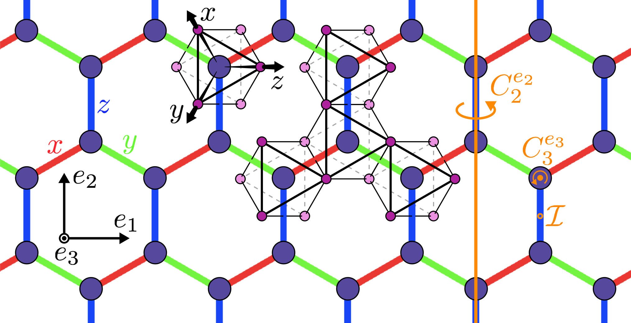
Figure 1: Honeycomb lattice of edge-sharing octahedra and its possible point group generating symmetries. The dark blue circles are magnetic metal ions, and the violet and pink circles surrounding them are ligands above and below the honeycomb plane, respectively, that form octahedra. Each metal ion interacts with its three neighboring metal ions through superexchange mediated by their shared non-magnetic ligands. This interaction is generally bond-dependent, so we can label the three different types of bonds as $x$-, $y$-, and $z$-bonds (shown in red, green, and blue, respectively). The three possible generating symmetries of the crystallographic point groups associated with this lattice are shown in orange. $C_{2}^{e_{2}}$ is the two-fold ($180^{\circ}$) rotational symmetry with respect to each $z$-bond axis, $C_{3}^{e_{3}}$ is the three-fold ($120^{\circ}$) rotational symmetry with respect to the out-of-plane axis through each site, and $\mathcal{I}$ is the inversion symmetry with respect to each bond center.

Crystal System	Point Group		Generating Symmetries	Examples of Materials
	Hermann–Mauguin Symbol	Schoenflies Symbol
Triclinic	$1$	$C_{1}$	$E$	—
	$\bar{1}$	$C_{i}$ ($S_{2}$)	$\mathcal{I}$	—
Monoclinic	$2$	$C_{2}$	$C_{2}^{e_{2}}$	—
	$2/m$	$C_{2h}$	$C_{2}^{e_{2}}$, $\mathcal{I}$	$\alpha$-RuCl3 Johnson et al. (2015), CrI3 McGuire et al. (2015), CrCl3 McGuire et al. (2017), Na2IrO3 Choi et al. (2012), $\alpha$-Li2IrO3 O’Malley et al. (2008), FePS3 Lee et al. (2016), IrCl3, IrBr3, IrI3, AlCl3, MoCl3, RhCl3, RhBr3, RhI3, TcCl3 McGuire (2017)
Trigonal	$3$	$C_{3}$	$C_{3}^{e_{3}}$	—
	$\bar{3}$	$C_{3i}$ ($S_{6}$)	$C_{3}^{e_{3}}$, $\mathcal{I}$	CrI3 McGuire et al. (2015); Ubrig et al. (2020), CrCl3 McGuire et al. (2017), CrBr3, VCl3, VBr3 McGuire (2017), VI3 Kong et al. (2019); Doležal et al. (2019), BiI3, FeCl3, TiCl3, TiBr3, Ti3O McGuire (2017), Cr2Ge2Te6 Carteaux et al. (1995), MnPSe3, FePSe3 Wiedenmann et al. (1981)
	$32$	$D_{3}$	$C_{2}^{e_{2}}$, $C_{3}^{e_{3}}$	FeCl3 McGuire (2017)
	$\bar{3}m$	$D_{3d}$	$C_{2}^{e_{2}}$, $C_{3}^{e_{3}}$, $\mathcal{I}$	—

Table 1: Generating symmetries and materials associated with the eight possible crystallographic point groups for the honeycomb lattices of edge-sharing octahedra. A given point group has rotation, reflection, and inversion symmetries that can be obtained from combinations of its generating symmetries. The symmetries $C_{2}^{e_{2}}$, $C_{3}^{e_{3}}$, $\mathcal{I}$ are described in Fig. 1, and the symmetry $E$ simply corresponds to the identity operation, which leaves the system unchanged (i.e., no rotation, reflection, or inversion). Trigonal crystals are sometimes referred to as rhombohedral, especially when they belong to a rhombohedral space group, such as $R\bar{3}$. Some materials are listed under more than one point group because can have different crystal structures depending on their temperature and sample thickness.

II.1 Two-Fold Rotational Symmetry ($C_{2}^{e_{2}}$)

The honeycomb lattice shown in Fig. 1 can have two-fold rotational symmetry (i.e., $180^{\circ}$ rotational symmetry) with respect to the armchair axis $e_{2}$ passing through each $z$-bond ($C_{2}^{e_{2}}$). This symmetry transformation corresponds to a rotation by $180^{\circ}$ with respect to the armchair axis $e_{2}$ and is described by the coordinate rotation matrix

$$\mathbf{C}_{2}^{e_{2}}=\begin{pmatrix}\cos(180^{\circ})&0&\sin(180^{\circ})\\ 0&1&0\\ -\sin(180^{\circ})&0&\cos(180^{\circ})\\ \end{pmatrix}=\begin{pmatrix}-1&0&0\\ 0&1&0\\ 0&0&-1\end{pmatrix}\,,$$ (2)

which effectively reverses a vector’s $e_{1}$ and $e_{3}$ components:

$$\begin{pmatrix}v_{e_{1}}\\ v_{e_{2}}\\ v_{e_{3}}\end{pmatrix}\xrightarrow{C_{2}^{e_{2}}}\mathbf{C}_{2}^{e_{2}}\begin{pmatrix}v_{e_{1}}\\ v_{e_{2}}\\ v_{e_{3}}\end{pmatrix}=\begin{pmatrix}-v_{e_{1}}\\ v_{e_{2}}\\ -v_{e_{3}}\end{pmatrix}\,.$$ (3)

We note that in crystals with $C_{2}^{e_{2}}$ symmetry (i.e., belonging to the monoclinic point groups $2$ or $2/m$, or to the trigonal point groups $32$, or $\bar{3}m$), the system’s $C_{2}^{e_{2}}$ symmetry can still be broken if it is magnetized along an axis that does not have $C_{2}$ symmetry.

II.2 Three-Fold Rotational Symmetry ($C_{3}^{e_{3}}$)

This lattice can also have three-fold rotational symmetry (i.e., $120^{\circ}$ rotational symmetry) with respect to the out-of-plane axis passing through each site ($C_{3}^{e_{3}}$). This symmetry transformation is described by the coordinate rotation matrix

$$\mathbf{C}_{3}^{e_{3}}=\begin{pmatrix}\cos(120^{\circ})&\sin(120^{\circ})&0\\ -\sin(120^{\circ})&\cos(120^{\circ})&0\\ 0&0&1\end{pmatrix}=\begin{pmatrix}-\frac{1}{2}&\frac{\sqrt{3}}{2}&0\\[2.0pt] -\frac{\sqrt{3}}{2}&-\frac{1}{2}&0\\[1.0pt] 0&0&1\end{pmatrix}\,,$$ (4)

which mixes a vector’s in-plane components:

$$\begin{pmatrix}v_{e_{1}}\\ v_{e_{2}}\\ v_{e_{3}}\end{pmatrix}\xrightarrow{C_{3}^{e_{3}}}\mathbf{C}_{3}^{e_{3}}\begin{pmatrix}v_{e_{1}}\\ v_{e_{2}}\\ v_{e_{3}}\end{pmatrix}=\begin{pmatrix}-\frac{1}{2}v_{e_{1}}+\frac{\sqrt{3}}{2}v_{e_{2}}\\[2.0pt] -\frac{\sqrt{3}}{2}v_{e_{1}}-\frac{1}{2}v_{e_{2}}\\ v_{e_{3}}\end{pmatrix}\,.$$ (5)

We note that in crystals with $C_{3}^{e_{3}}$ symmetry (i.e., belonging to the trigonal point groups $3$, $\bar{3}$, $32$ and $\bar{3}m$), the system’s $C_{3}^{e_{3}}$ symmetry can still be broken if it is magnetized along an axis other than the out-of-plane axis.

We now clarify a possible point of confusion in our definition of the in-plane axes $e_{1}$ and $e_{2}$. For systems with $C_{2}^{e_{2}}$ symmetry but without $C_{3}^{e_{3}}$ symmetry (i.e., belonging to the monoclinic point groups $2$ and $2/m$), there are two different types of armchair axes: the unique armchair axis that has $C_{2}$ symmetry, and the other two equivalent armchair axes that do not have this symmetry (see Fig. 2). For these systems, we define $e_{2}$ as this unique high-symmetry armchair axis, and similarly we define $z$-bonds as the bonds oriented along this axis. For systems with $C_{3}^{e_{3}}$ symmetry (i.e., belonging to the trigonal point groups $3$, $\bar{3}$, $32$ and $\bar{3}m$), the three armchair axes are equivalent, so we arbitrarily define $e_{2}$ as any one of these axes. Finally, for systems without $C_{2}^{e_{2}}$ or $C_{3}^{e_{3}}$ symmetry (i.e., belonging to the triclinic point groups $1$ and $\bar{1}$), the three armchair axes are all different, so we again arbitrarily define $e_{2}$ as any one of these axes. In all of these cases, we define $e_{1}$ as the zigzag axis perpendicular to the $e_{2}$-axis.

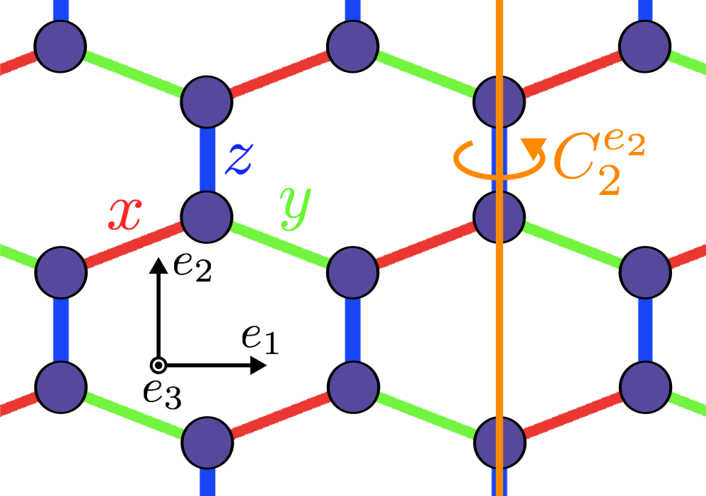
Figure 2: Honeycomb lattice for a monoclinic crystal (point groups $2$ or $2/m$). This lattice lacks three-fold ($120^{\circ}$) rotational symmetry because $z$-bonds do not have the same length as $x$- and $y$-bonds, and it has two-fold ($180^{\circ}$) rotational symmetry because $x$- and $y$-bonds have the same length. The high-symmetry armchair axis (shown in orange) along $z$-bonds therefore has two-fold rotational symmetry, whereas the other two armchair axes along $x$- and $y$-bonds lack this symmetry.

II.3 Inversion Symmetry ($\mathcal{I}$)

Finally, this system can also have bond-centered inversion symmetry ($\mathcal{I}$). Under inversion, vectors transform as

$$\mathbf{v}\xrightarrow{\mathcal{I}}\lambda_{\mathcal{I}}\mathbf{v}\,,$$ (6)

where the eigenvalue $\lambda_{\mathcal{I}}=\pm 1$ depends on the particular vector $\mathbf{v}$. Vectors that are odd under inversion ($\lambda_{\mathcal{I}}=-1$) are called polar vectors and include quantities such as electric field, electric current, temperature gradient, heat current, spin current, and momentum, whereas vectors that are even under inversion ($\lambda_{\mathcal{I}}=+1$) are called axial vectors (or pseudovectors) and include quantities like magnetic field, magnetization, and spin.

A more common way of describing how vectors transform under inversion is using the coordinate inversion matrix

$$\boldsymbol{\mathcal{I}}=\begin{pmatrix}-1&0&0\\ 0&-1&0\\ 0&0&-1\end{pmatrix}$$ (7)

and using the transformation rules

$$\mathbf{v} \xrightarrow{\mathcal{I}}\boldsymbol{\mathcal{I}}\mathbf{v}=-\mathbf{v}\quad \text{(polar vector)}\,,$$ (8)

$$\mathbf{v} \xrightarrow{\mathcal{I}}|\boldsymbol{\mathcal{I}}|\boldsymbol{\mathcal{I}}\mathbf{v}=\mathbf{v}\quad \hskip 1.0pt\text{(axial vector)}\,,$$

where $|\boldsymbol{\mathcal{I}}|=-1$ is the determinant of the transformation matrix $\boldsymbol{\mathcal{I}}$. This formulation is useful because it allows us to generalize the transformation rules for polar and axial vectors under any orthogonal transformation matrix $\mathbf{R}$ as

$$\mathbf{v} \xrightarrow{R}\mathbf{R}\mathbf{v}\quad \text{(polar vector)}\,,$$ (9)

$$\mathbf{v} \xrightarrow{R}|\mathbf{R}|\mathbf{R}\mathbf{v}\quad \hskip 1.0pt\text{(axial vector)}\,,$$

where transformation matrices with $|\mathbf{R}|=+1$ describe rotations, whereas those with $|\mathbf{R}|=-1$ describe improper rotations (i.e., the combination of a rotation and an inversion).

III Zero-Field Tensors

In this section we describe the general forms of tensors allowed by the symmetries described earlier for systems with no external magnetic or electric fields, and as an example we discuss and make testable predictions for the magnetic field derivative of the thermal conductivity tensor, $(\partial\kappa_{ij}/\partial H_{k})|_{\mathbf{H}=\mathbf{0}}$.

Generating Symmetry	Rank-2 Tensors (no external field)	Rank-3 Tensors (no external field)	Rank-$r$ Tensors (no external field)
$C_{2}^{e_{2}}$	$T_{e_{1}e_{2}}=T_{e_{2}e_{1}}=T_{e_{2}e_{3}}=T_{e_{3}e_{2}}=0$	$T_{e_{1}e_{1}e_{1}}=T_{e_{3}e_{3}e_{3}}=0$ $T_{e_{1}e_{1}e_{3}}=T_{e_{1}e_{3}e_{1}}=T_{e_{3}e_{1}e_{1}}=0$ $T_{e_{3}e_{3}e_{1}}=T_{e_{3}e_{1}e_{3}}=T_{e_{1}e_{3}e_{3}}=0$ $T_{e_{1}e_{2}e_{2}}=T_{e_{2}e_{1}e_{2}}=T_{e_{2}e_{2}e_{1}}=0$  $T_{e_{3}e_{2}e_{2}}=T_{e_{2}e_{3}e_{2}}=T_{e_{2}e_{2}e_{3}}=0$	$T_{i_{1}i_{2}\ldots i_{r}}=0$ if $N_{e_{1}}+N_{e_{3}}$ is odd ($N_{\alpha}=$ # of indices equal to $\alpha$)
$C_{3}^{e_{3}}$	$T_{e_{1}e_{1}}=T_{e_{2}e_{2}}$ $T_{e_{1}e_{2}}=-T_{e_{2}e_{1}}$ $T_{e_{1}e_{3}}=T_{e_{3}e_{1}}=T_{e_{2}e_{3}}=T_{e_{3}e_{2}}=0$	$T_{e_{1}e_{1}e_{1}}=-T_{e_{1}e_{2}e_{2}}=-T_{e_{2}e_{1}e_{2}}=-T_{e_{2}e_{2}e_{1}}$ $T_{e_{2}e_{2}e_{2}}=-T_{e_{2}e_{1}e_{1}}=-T_{e_{1}e_{2}e_{1}}=-T_{e_{1}e_{1}e_{2}}$ $T_{e_{1}e_{1}e_{3}}=T_{e_{2}e_{2}e_{3}}$ $T_{e_{1}e_{3}e_{1}}=T_{e_{2}e_{3}e_{2}}$ $T_{e_{3}e_{1}e_{1}}=T_{e_{3}e_{2}e_{2}}$ $T_{e_{1}e_{2}e_{3}}=-T_{e_{2}e_{1}e_{3}}$ $T_{e_{1}e_{3}e_{2}}=-T_{e_{2}e_{3}e_{1}}$ $T_{e_{3}e_{2}e_{1}}=-T_{e_{3}e_{1}e_{2}}$ $T_{e_{1}e_{3}e_{3}}=T_{e_{3}e_{1}e_{3}}=T_{e_{3}e_{3}e_{1}}=0$ $T_{e_{2}e_{3}e_{3}}=T_{e_{3}e_{2}e_{3}}=T_{e_{3}e_{3}e_{2}}=0$	No simple constraint
$\mathcal{I}$	$T_{ij}=0$ if exactly one of the indices $(i,j)$ corresponds to a polar vector	$T_{ijk}=0$ if exactly one or three of the indices $(i,j,k)$ correspond to polar vectors	$T_{i_{1}i_{2}\ldots i_{r}}=0$ if the number of indices corresponding to polar vectors is odd

Table 2: Constraints imposed by the point group generating symmetries on zero-field tensors. These symmetries are described in Fig. 1.

III.1 Rank-2 Tensors

We can express a general rank-2 tensor $T_{ij}$ for a system with no external field as a $3\times 3$ matrix in $e_{1}e_{2}e_{3}$ coordinates as

$$T_{ij}=\begin{pmatrix}T_{e_{1}e_{1}}&T_{e_{1}e_{2}}&T_{e_{1}e_{3}}\\ T_{e_{2}e_{1}}&T_{e_{2}e_{2}}&T_{e_{2}e_{3}}\\ T_{e_{3}e_{1}}&T_{e_{3}e_{2}}&T_{e_{3}e_{3}}\end{pmatrix}\,.$$ (10)

Under an orthogonal transformation matrix $\mathbf{R}$, rank-2 tensors transform as 

$$T_{ij}\xrightarrow{R}|\mathbf{R}|^{N_{\text{axial}}}R_{im}R_{jn}T_{mn}\,,$$ (11)

where $N_{\text{axial}}$ is the number of indices in the tensor $T$ corresponding to axial vectors. In matrix notation, this equation is

$$\mathbf{T}\xrightarrow{R}|\mathbf{R}|^{N_{\text{axial}}}\mathbf{R}\mathbf{T}\mathbf{R}^{\mathrm{T}}\,,$$ (12)

where $\mathbf{R}^{\mathrm{T}}$ denotes the transpose of $\mathbf{R}$.

For example, under $C_{2}^{e_{2}}$, rank-2 tensors transform as

$$\mathbf{T}\xrightarrow{C_{2}^{e_{2}}}\mathbf{T}^{\prime}=\mathbf{C}_{2}^{e_{2}}\mathbf{T}(\mathbf{C}_{2}^{e_{2}})^{\mathrm{T}}\,,$$ (13)

or explicitly,

$$\begin{pmatrix}T^{\prime}_{e_{1}e_{1}}&T^{\prime}_{e_{1}e_{2}}&T^{\prime}_{e_{1}e_{3}}\\ T^{\prime}_{e_{2}e_{1}}&T^{\prime}_{e_{2}e_{2}}&T^{\prime}_{e_{2}e_{3}}\\ T^{\prime}_{e_{3}e_{1}}&T^{\prime}_{e_{3}e_{2}}&T^{\prime}_{e_{3}e_{3}}\end{pmatrix}=\begin{pmatrix}T_{e_{1}e_{1}}&-T_{e_{1}e_{2}}&T_{e_{1}e_{3}}\\ -T_{e_{2}e_{1}}&T_{e_{2}e_{2}}&-T_{e_{2}e_{3}}\\ T_{e_{3}e_{1}}&-T_{e_{3}e_{2}}&T_{e_{3}e_{3}}\end{pmatrix}\,.$$ (14)

Invariance under this transformation ($T_{ij}=T^{\prime}_{ij}$) imposes the constraints

$$T_{e_{1}e_{2}}=T_{e_{2}e_{1}}=T_{e_{2}e_{3}}=T_{e_{3}e_{2}}=0\,.\qquad(C_{2}^{e_{2}})$$ (15)

Similarly, $C_{3}^{e_{3}}$ imposes the constraints

$$\begin{aligned} T_{e_{1}e_{1}}&=T_{e_{2}e_{2}}\,,\\ T_{e_{1}e_{2}}&=-T_{e_{2}e_{1}}\,,\\ T_{e_{1}e_{3}}=T_{e_{3}e_{1}}&=T_{e_{2}e_{3}}=T_{e_{3}e_{2}}=0\,.\end{aligned}\qquad(C_{3}^{e_{3}})$$ (16)

We note that for systems with $C_{3}^{e_{3}}$ symmetry, rank-2 zero-field tensors have continuous rotational symmetry with respect to the axis perpendicular to the plane, since they are invariant upon rotating the orientation of the in-plane axes $e_{1}$ and $e_{2}$ to point along any two perpendicular directions inside the plane:

$$\begin{pmatrix}\cos\theta&\sin\theta&0\\ -\sin\theta&\cos\theta&0\\ 0&0&1\end{pmatrix}\mathbf{T}\begin{pmatrix}\cos\theta&\sin\theta&0\\ -\sin\theta&\cos\theta&0\\ 0&0&1\end{pmatrix}^{\mathrm{T}}=\mathbf{T}\,.$$ (17)

In these systems, rank-2 physical responses (such as the magnetic susceptibility $\chi_{ij}=(\partial M_{i}/\partial H_{j})|_{\mathbf{H}=\mathbf{0}}$) therefore behave the same way along all in-plane directions Andrade et al. (2020), including low-symmetry directions.

Finally, inversion symmetry does not constrain the form of rank-2 tensors, but it does require that either none or both of the tensor indices ($i,j$) correspond to polar vectors, otherwise the tensor will equal zero.

The most general forms of rank-2 zero-field tensors for systems belonging to the eight point groups generated by these three symmetries (see Table 1) are given in Table 3.

III.2 Rank-3 Tensors

Higher-rank tensors, such as rank-3 tensors, can arise in a multilinear manner as a linear response to multiple perturbations, such as the bilinear response of the magnetization to a thermal gradient and an applied magnetic field. In addition, higher-rank tensors are necessary to describe higher-order or nonlinear responses to a perturbation.

We can express a general rank-3 tensor $T_{ijk}$ for a system with no external field as a set of three $3\times 3$ matrices in $e_{1}e_{2}e_{3}$ coordinates as

$$T_{e_{1}jk} =\begin{pmatrix}T_{e_{1}e_{1}e_{1}}&T_{e_{1}e_{1}e_{2}}&T_{e_{1}e_{1}e_{3}}\\ T_{e_{1}e_{2}e_{1}}&T_{e_{1}e_{2}e_{2}}&T_{e_{1}e_{2}e_{3}}\\ T_{e_{1}e_{3}e_{1}}&T_{e_{1}e_{3}e_{2}}&T_{e_{1}e_{3}e_{3}}\end{pmatrix}\,,$$ (18)

$$T_{e_{2}jk} =\begin{pmatrix}T_{e_{2}e_{1}e_{1}}&T_{e_{2}e_{1}e_{2}}&T_{e_{2}e_{1}e_{3}}\\ T_{e_{2}e_{2}e_{1}}&T_{e_{2}e_{2}e_{2}}&T_{e_{2}e_{2}e_{3}}\\ T_{e_{2}e_{3}e_{1}}&T_{e_{2}e_{3}e_{2}}&T_{e_{2}e_{3}e_{3}}\end{pmatrix}\,,$$

$$T_{e_{3}jk} =\begin{pmatrix}T_{e_{3}e_{1}e_{1}}&T_{e_{3}e_{1}e_{2}}&T_{e_{3}e_{1}e_{3}}\\ T_{e_{3}e_{2}e_{1}}&T_{e_{3}e_{2}e_{2}}&T_{e_{3}e_{2}e_{3}}\\ T_{e_{3}e_{3}e_{1}}&T_{e_{3}e_{3}e_{2}}&T_{e_{3}e_{3}e_{3}}\end{pmatrix}\,.$$

Under an orthogonal transformation described by a matrix $R_{ij}$, rank-3 tensors transform as

$$T_{ijk}\xrightarrow{R}|\mathbf{R}|^{N_{\text{axial}}}R_{i\ell}R_{jm}R_{kn}T_{\ell mn}\,,$$ (19)

or, in matrix notation,

$$\mathbf{T}_{i}\xrightarrow{R}|\mathbf{R}|^{N_{\text{axial}}}R_{i\ell}\mathbf{R}\mathbf{T}_{\ell}\mathbf{R}^{\mathrm{T}}\,,$$ (20)

where $\mathbf{T}_{i}$ is the matrix representation of $T_{ijk}$ for a given $i$.

$C_{2}^{e_{2}}$ symmetry imposes the constraints

$$\hskip 30.5pt\begin{aligned} T_{e_{1}e_{1}e_{1}}=T_{e_{3}e_{3}e_{3}}&=0\,,\\ T_{e_{1}e_{1}e_{3}}=T_{e_{1}e_{3}e_{1}}=T_{e_{3}e_{1}e_{1}}&=0\,,\\ T_{e_{3}e_{3}e_{1}}=T_{e_{3}e_{1}e_{3}}=T_{e_{1}e_{3}e_{3}}&=0\,,\\ T_{e_{1}e_{2}e_{2}}=T_{e_{2}e_{1}e_{2}}=T_{e_{2}e_{2}e_{1}}&=0\,,\\ T_{e_{3}e_{2}e_{2}}=T_{e_{2}e_{3}e_{2}}=T_{e_{2}e_{2}e_{3}}&=0\,,\end{aligned}\qquad(C_{2}^{e_{2}})$$ (21)

and $C_{3}^{e_{3}}$ symmetry imposes the constraints

$$\begin{aligned} T_{e_{1}e_{1}e_{1}}=-T_{e_{1}e_{2}e_{2}}&=-T_{e_{2}e_{1}e_{2}}=-T_{e_{2}e_{2}e_{1}}\,,\\ T_{e_{2}e_{2}e_{2}}=-T_{e_{2}e_{1}e_{1}}&=-T_{e_{1}e_{2}e_{1}}=-T_{e_{1}e_{1}e_{2}}\,,\\ T_{e_{1}e_{1}e_{3}}&=T_{e_{2}e_{2}e_{3}}\,,\\ T_{e_{1}e_{3}e_{1}}&=T_{e_{2}e_{3}e_{2}}\,,\\ T_{e_{3}e_{1}e_{1}}&=T_{e_{3}e_{2}e_{2}}\,,\\ T_{e_{1}e_{2}e_{3}}&=-T_{e_{2}e_{1}e_{3}}\,,\\ T_{e_{1}e_{3}e_{2}}&=-T_{e_{2}e_{3}e_{1}}\,,\\ T_{e_{3}e_{2}e_{1}}&=-T_{e_{3}e_{1}e_{2}}\,,\\ T_{e_{1}e_{3}e_{3}}&=T_{e_{3}e_{1}e_{3}}=T_{e_{3}e_{3}e_{1}}=0\,,\\ T_{e_{2}e_{3}e_{3}}&=T_{e_{3}e_{2}e_{3}}=T_{e_{3}e_{3}e_{2}}=0\,.\end{aligned}(C_{3}^{e_{3}})$$ (22)

Remarkably, for systems with $C_{3}^{e_{3}}$ symmetry, the fully longitudinal components along the zigzag and armchair in-plane directions $e_{1}$ and $e_{2}$ (namely $T_{e_{1}e_{1}e_{1}}$ and $T_{e_{2}e_{2}e_{2}}$) are equal in magnitude to some partly transverse components along these in-plane directions, as we can see in the first two lines in the equations above, namely

$$T_{e_{1}e_{1}e_{1}}=-T_{e_{1}e_{2}e_{2}} =-T_{e_{2}e_{1}e_{2}}=-T_{e_{2}e_{2}e_{1}}\,,$$ (23)

$$T_{e_{2}e_{2}e_{2}}=-T_{e_{2}e_{1}e_{1}} =-T_{e_{1}e_{2}e_{1}}=-T_{e_{1}e_{1}e_{2}}\,.$$ (24)

For example, although one might have expected that $T_{e_{2}e_{2}e_{2}}$ and $T_{e_{2}e_{1}e_{1}}$ describe different physical processes and therefore have different values, $C_{3}^{e_{3}}$ symmetry nevertheless requires them to be the same. We note that in systems that also have $C_{2}^{e_{2}}$ symmetry, the tensor components in Eq. 23 (but not those in Eq. 24) will be zero, so we expect that in systems with small distortions that weakly break $C_{2}^{e_{2}}$ symmetry, the components in Eq. 23 will be relatively small.

Unlike with rank-2 zero-field tensors, rank-3 zero-field tensors describing systems with $C_{3}^{e_{3}}$ symmetry do not generally have continuous rotational symmetry with respect to the axis perpendicular to the plane. In fact, for systems with $C_{3}^{e_{3}}$ or $C_{2}^{e_{2}}$ symmetry, the in-plane zigzag and armchair directions $e_{1}$ and $e_{2}$ generally behave differently for rank-3 zero-field tensors, so rank-3 tensors are more sensitive at probing differences directional differences within the plane.

Finally, inversion symmetry again does not constrain the form of rank-3 tensors, but it imposes that either none or two of the tensor indices correspond to the polar vectors, otherwise the tensor will equal zero.

The most general forms of rank-3 zero-field tensors for the eight point groups generated by these three symmetries are given in Table 3.

III.2.1 Example: Thermomagnetic Susceptibility Tensor $\chi^{\text{thermomag}}_{ijk}$

An example of a rank-3 zero-field tensor is the thermomagnetic susceptibility tensor

$$\chi^{\text{thermomag}}_{ijk}=\frac{\partial\kappa_{ij}}{\partial H_{k}}\biggr{|}_{\mathbf{H}=\mathbf{0}}\,,\vspace{-3pt}$$ (25)

Point Groups	Rank-2 Tensors (no external field)	Rank-3 Tensors (no external field)	Thermal Conductivity Tensor (in external magnetic field $\mathbf{H}$)
$1$,  $\bar{1}$	$T_{ij}=\begin{pmatrix}A&B&C\\ D&E&F\\ G&I&J\\ \vspace{-13.6pt}\hphantom{-B}&\hphantom{B}&\hphantom{-B}\end{pmatrix}$	$T_{e_{1}jk}=\begin{pmatrix}A_{1}&B_{1}&C_{1}\\ D_{1}&E_{1}&F_{1}\\ G_{1}&I_{1}&J_{1}\\ \vspace{-13.6pt}\hphantom{-D}&\hphantom{-B}&\hphantom{-D}\end{pmatrix}$ $T_{e_{2}jk}=\begin{pmatrix}A_{2}&B_{2}&C_{2}\\ D_{2}&E_{2}&F_{2}\\ G_{2}&I_{2}&J_{2}\\ \vspace{-13.6pt}\hphantom{-D}&\hphantom{-B}&\hphantom{-D}\end{pmatrix}$ $T_{e_{3}jk}=\begin{pmatrix}A_{3}&B_{3}&C_{3}\\ D_{3}&E_{3}&F_{3}\\ G_{3}&I_{3}&J_{3}\\ \vspace{-13.6pt}\hphantom{-D}&\hphantom{-B}&\hphantom{-D}\end{pmatrix}$	$\kappa_{ij}(H\hat{\mathbf{e}}_{1})=\overset{\overset{\textbf{\small Even in $H$}}{\vphantom{,}}}{\begin{pmatrix}A_{1}&B_{1}&C_{1}\\ B_{1}&D_{1}&E_{1}\\ C_{1}&E_{1}&F_{1}\\ \vspace{-13.6pt}\hphantom{B_{3}}&\hphantom{D_{3}}&\hphantom{B_{3}}\end{pmatrix}}+\overset{\overset{\textbf{\small Odd in $H$}}{\vphantom{,}}}{\begin{pmatrix}0&G_{1}&I_{1}\\ -G_{1}&0&J_{1}\\ -I_{1}&-J_{1}&0\\ \vspace{-13.6pt}\hphantom{-G_{3}}&\hphantom{-J_{3}}&\hphantom{-J_{3}}\end{pmatrix}}$ $\kappa_{ij}(H\hat{\mathbf{e}}_{2})=\begin{pmatrix}A_{2}&B_{2}&C_{2}\\ B_{2}&D_{2}&E_{2}\\ C_{2}&E_{2}&F_{2}\\ \vspace{-13.6pt}\hphantom{B_{3}}&\hphantom{D_{3}}&\hphantom{B_{3}}\end{pmatrix}+\begin{pmatrix}0&G_{2}&I_{2}\\ -G_{2}&0&J_{2}\\ -I_{2}&-J_{2}&0\\ \vspace{-13.6pt}\hphantom{-G_{3}}&\hphantom{-J_{3}}&\hphantom{-J_{3}}\end{pmatrix}$ $\kappa_{ij}(H\hat{\mathbf{e}}_{3})=\begin{pmatrix}A_{3}&B_{3}&C_{3}\\ B_{3}&D_{3}&E_{3}\\ C_{3}&E_{3}&F_{3}\\ \vspace{-13.6pt}\hphantom{B_{3}}&\hphantom{D_{3}}&\hphantom{B_{3}}\end{pmatrix}+\begin{pmatrix}0&G_{3}&I_{3}\\ -G_{3}&0&J_{3}\\ -I_{3}&-J_{3}&0\\ \vspace{-13.6pt}\hphantom{-G_{3}}&\hphantom{-J_{3}}&\hphantom{-J_{3}}\end{pmatrix}$
$2$,  $2/m$	$T_{ij}=\begin{pmatrix}A&0&B\\ 0&C&0\\ D&0&E\\ \vspace{-13.6pt}\hphantom{-B}&\hphantom{B}&\hphantom{-B}\end{pmatrix}$	$T_{e_{1}jk}=\begin{pmatrix}0&A&0\\ B&0&C\\ 0&D&0\\ \vspace{-13.6pt}\hphantom{-D}&\hphantom{-B}&\hphantom{-D}\end{pmatrix}$ $T_{e_{2}jk}=\begin{pmatrix}E&0&F\\ 0&G&0\\ I&0&J\\ \vspace{-13.6pt}\hphantom{-D}&\hphantom{-B}&\hphantom{-D}\end{pmatrix}$ $T_{e_{3}jk}=\begin{pmatrix}0&K&0\\ L&0&M\\ 0&N&0\\ \vspace{-13.6pt}\hphantom{-D}&\hphantom{-B}&\hphantom{-D}\end{pmatrix}$	$\kappa_{ij}(H\hat{\mathbf{e}}_{1})=\overset{\overset{\textbf{\small Even in $H$}}{\vphantom{,}}}{\begin{pmatrix}A&0&B\\ 0&C&0\\ B&0&D\\ \vspace{-13.6pt}\hphantom{B_{3}}&\hphantom{D_{3}}&\hphantom{B_{3}}\end{pmatrix}}+\overset{\overset{\textbf{\small Odd in $H$}}{\vphantom{,}}}{\begin{pmatrix}0&E&0\\ -E&0&F\\ 0&-F&0\\ \vspace{-13.6pt}\hphantom{-G_{3}}&\hphantom{-J_{3}}&\hphantom{-J_{3}}\end{pmatrix}}$ $\kappa_{ij}(H\hat{\mathbf{e}}_{2})=\begin{pmatrix}G&0&I\\ 0&J&0\\ I&0&K\\ \vspace{-13.6pt}\hphantom{B_{3}}&\hphantom{D_{3}}&\hphantom{B_{3}}\end{pmatrix}+\begin{pmatrix}0&0&L\\ 0&0&0\\ -L&0&0\\ \vspace{-13.6pt}\hphantom{-G_{3}}&\hphantom{-J_{3}}&\hphantom{-J_{3}}\end{pmatrix}$ $\kappa_{ij}(H\hat{\mathbf{e}}_{3})=\begin{pmatrix}M&0&N\\ 0&P&0\\ N&0&Q\\ \vspace{-13.6pt}\hphantom{B_{3}}&\hphantom{D_{3}}&\hphantom{B_{3}}\end{pmatrix}+\begin{pmatrix}0&R&0\\ -R&0&S\\ 0&-S&0\\ \vspace{-13.6pt}\hphantom{-G_{3}}&\hphantom{-J_{3}}&\hphantom{-J_{3}}\end{pmatrix}$
$3$,  $\bar{3}$	$T_{ij}=\begin{pmatrix}A&B&0\\ -B&A&0\\ 0&0&C\\ \vspace{-13.6pt}\hphantom{-B}&\hphantom{B}&\hphantom{-B}\end{pmatrix}$	$T_{e_{1}jk}=\begin{pmatrix}A&B&C\\ B&-A&D\\ E&F&0\\ \vspace{-13.6pt}\hphantom{-D}&\hphantom{-B}&\hphantom{-D}\end{pmatrix}$ $T_{e_{2}jk}=\begin{pmatrix}B&-A&-D\\ -A&-B&C\\ -F&E&0\\ \vspace{-13.6pt}\hphantom{-D}&\hphantom{-B}&\hphantom{-D}\end{pmatrix}$ $T_{e_{3}jk}=\begin{pmatrix}G&I&0\\ -I&G&0\\ 0&0&J\\ \vspace{-13.6pt}\hphantom{-D}&\hphantom{-B}&\hphantom{-D}\end{pmatrix}$	$\kappa_{ij}(H\hat{\mathbf{e}}_{1})=\overset{\overset{\textbf{\small Even in $H$}}{\vphantom{,}}}{\begin{pmatrix}A&B&C\\ B&D&E\\ C&E&F\\ \vspace{-13.6pt}\hphantom{B_{3}}&\hphantom{D_{3}}&\hphantom{B_{3}}\end{pmatrix}}+\overset{\overset{\textbf{\small Odd in $H$}}{\vphantom{,}}}{\begin{pmatrix}0&G&I\\ -G&0&J\\ -I&-J&0\\ \vspace{-13.6pt}\hphantom{-G_{3}}&\hphantom{-J_{3}}&\hphantom{-J_{3}}\end{pmatrix}}$ $\kappa_{ij}(H\hat{\mathbf{e}}_{2})=\begin{pmatrix}K&L&M\\ L&N&P\\ M&P&Q\\ \vspace{-13.6pt}\hphantom{B_{3}}&\hphantom{D_{3}}&\hphantom{B_{3}}\end{pmatrix}+\begin{pmatrix}0&R&S\\ -R&0&T\\ -S&-T&0\\ \vspace{-13.6pt}\hphantom{-G_{3}}&\hphantom{-J_{3}}&\hphantom{-J_{3}}\end{pmatrix}$ $\kappa_{ij}(H\hat{\mathbf{e}}_{3})=\begin{pmatrix}U&0&0\\ 0&U&0\\ 0&0&V\\ \vspace{-13.6pt}\hphantom{B_{3}}&\hphantom{D_{3}}&\hphantom{B_{3}}\end{pmatrix}+\begin{pmatrix}0&W&0\\ -W&0&0\\ 0&0&0\\ \vspace{-13.6pt}\hphantom{-G_{3}}&\hphantom{-J_{3}}&\hphantom{-J_{3}}\end{pmatrix}$
$32$,  $\bar{3}m$	$T_{ij}=\begin{pmatrix}A&0&0\\ 0&A&0\\ 0&0&B\\ \vspace{-13.6pt}\hphantom{-B}&\hphantom{B}&\hphantom{-B}\end{pmatrix}$	$T_{e_{1}jk}=\begin{pmatrix}0&A&0\\ A&0&B\\ 0&C&0\\ \vspace{-13.6pt}\hphantom{-D}&\hphantom{-B}&\hphantom{-D}\end{pmatrix}$ $T_{e_{2}jk}=\begin{pmatrix}A&0&-B\\ 0&-A&0\\ -C&0&0\\ \vspace{-13.6pt}\hphantom{-D}&\hphantom{-B}&\hphantom{-D}\end{pmatrix}$ $T_{e_{3}jk}=\begin{pmatrix}0&D&0\\ -D&0&0\\ 0&0&0\\ \vspace{-13.6pt}\hphantom{-D}&\hphantom{-B}&\hphantom{-D}\end{pmatrix}$	$\kappa_{ij}(H\hat{\mathbf{e}}_{1})=\overset{\overset{\textbf{\small Even in $H$}}{\vphantom{,}}}{\begin{pmatrix}A&0&B\\ 0&C&0\\ B&0&D\\ \vspace{-13.6pt}\hphantom{B_{3}}&\hphantom{D_{3}}&\hphantom{B_{3}}\end{pmatrix}}+\overset{\overset{\textbf{\small Odd in $H$}}{\vphantom{,}}}{\begin{pmatrix}0&E&0\\ -E&0&F\\ 0&-F&0\\ \vspace{-13.6pt}\hphantom{-G_{3}}&\hphantom{-J_{3}}&\hphantom{-J_{3}}\end{pmatrix}}$ $\kappa_{ij}(H\hat{\mathbf{e}}_{2})=\begin{pmatrix}G&0&I\\ 0&J&0\\ I&0&K\\ \vspace{-13.6pt}\hphantom{B_{3}}&\hphantom{D_{3}}&\hphantom{B_{3}}\end{pmatrix}+\begin{pmatrix}0&0&L\\ 0&0&0\\ -L&0&0\\ \vspace{-13.6pt}\hphantom{-G_{3}}&\hphantom{-J_{3}}&\hphantom{-J_{3}}\end{pmatrix}$ $\kappa_{ij}(H\hat{\mathbf{e}}_{3})=\begin{pmatrix}M&0&0\\ 0&M&0\\ 0&0&N\\ \vspace{-13.6pt}\hphantom{B_{3}}&\hphantom{D_{3}}&\hphantom{B_{3}}\end{pmatrix}+\begin{pmatrix}0&P&0\\ -P&0&0\\ 0&0&0\\ \vspace{-13.6pt}\hphantom{-G_{3}}&\hphantom{-J_{3}}&\hphantom{-J_{3}}\end{pmatrix}$

Table 3: General forms of rank-2 and rank-3 tensors in systems with no external field (magnetic or electric) and of the thermal conductivity tensor $\kappa_{ij}(\mathbf{H})$ in systems with an external magnetic field $\mathbf{H}$ along the high-symmetry directions $\alpha=e_{1},e_{2},e_{3}$ ($e_{1}$ = in-plane zigzag direction, $e_{2}$ = in-plane armchair direction, $e_{3}$ = out-of-plane direction; see Fig. 1) for systems of various point groups. The components of these tensors are expressed in $e_{1}e_{2}e_{3}$ coordinates (e.g., see Eqs. 10 and 18). The components of the thermal conductivity tensor that are even functions of $H$ correspond to the thermomagnetic conductivity, whereas those that are odd functions of $H$ correspond to the thermal Hall conductivity.

where $\kappa_{ij}$ is the thermal conductivity tensor, defined by

$$(J_{Q})_{i}=-\kappa_{ij}\nabla_{j}T\,,$$ (26)

$\mathbf{J}_{Q}$ is the heat current, $\boldsymbol{\nabla}T$ is the temperature gradient, and $\mathbf{H}$ is the external magnetic field. Even though we are taking a magnetic field derivative, this is still a zero-field tensor because we are evaluating the derivative in the zero-field limit (i.e., the infinitesimally small field is only being used to probe the zero-field ground state). Also note that while $\chi^{\text{thermomag}}_{ijk}$ is linear in the vectors $\mathbf{H}$ and $\boldsymbol{\nabla}T$, rank-3 tensors can also be quadratic in a given vector, such as the nonlinear magnetic susceptibility tensor Shivaram (2014); Shivaram et al. (2014, 2017, 2018)

$$\chi^{\text{nonlinear}}_{ijk}=\frac{\partial^{2}M_{i}}{\partial H_{j}\partial H_{k}}\,,$$ (27)

which is quadratic in $\mathbf{H}$.

For a material with $C_{3}^{e_{3}}$ symmetry, such as CrI₃ in the rhombohedral configuration $R\bar{3}$ McGuire et al. (2015); Ubrig et al. (2020), we expect that $\chi^{\text{thermomag}}_{e_{1}e_{2}e_{1}}=-\chi^{\text{thermomag}}_{e_{2}e_{2}e_{2}}$ (see Eq. 24), or more explicitly,

$$\frac{\partial\kappa_{e_{1}e_{2}}}{\partial H_{e_{1}}}\biggr{|}_{\mathbf{H}=\mathbf{0}}=-\frac{\partial\kappa_{e_{2}e_{2}}}{\partial H_{e_{2}}}\biggr{|}_{\mathbf{H}=\mathbf{0}}\,.$$ (28)

This result is surprising because the left side corresponds to the field derivative of a thermal Hall conductivity ($\mathbf{J}_{Q}\perp\boldsymbol{\nabla}T$) (Fig. 3a), whereas the right side corresponds to the field derivative of a longitudinal thermal conductivity ($\mathbf{J}_{Q}\parallel\boldsymbol{\nabla}T$) (Fig. 3b). These results still hold when the system is magnetized along the out-of-plane direction, as this does not break $C_{3}^{e_{3}}$ symmetry. We can obtain several other similar expressions using Eqs. 23 and 24.

Note that even though components such as $\chi^{\text{thermomag}}_{e_{3}e_{1}e_{2}}$ and $\chi^{\text{thermomag}}_{e_{1}e_{3}e_{2}}$ are always allowed to be nonzero for all eight point groups possible, we nevertheless expect them to be zero for monolayer systems, since heat currents and temperature gradients cannot physically be oriented perpendicular to a 2D system . We therefore only expect these components to become relevant for bulk systems.

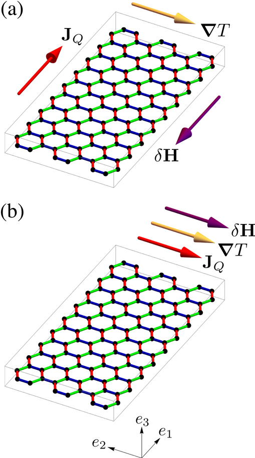
Figure 3: Example illustrating one of the unusual equalities for rank-3 tensors describing crystals with $C_{3}^{e_{3}}$ symmetry (i.e., belonging to the trigonal point groups $3$, $\bar{3}$, $32$, or $\bar{3}m$). In the absence of external magnetic or electric fields, (a) the change in the thermal Hall conductivity $\delta\kappa_{e_{1}e_{2}}$ that results from applying a small magnetic field $\delta\mathbf{H}$ along the zigzag direction $e_{1}$ will be the same as (b) the change in the longitudinal thermal conductivity $\delta\kappa_{e_{2}e_{2}}$ that results from applying a small magnetic field $\delta\mathbf{H}$ along the armchair direction $e_{2}$ (Eq. 28). $\mathbf{J}_{Q}$ is the heat current and $\boldsymbol{\nabla}T$ is the temperature gradient. Reversing the direction of any one of the three vectors simply reverses the sign of the change in the thermal conductivity. These results hold when the system is either not magnetized, or magnetized along the out-of-plane direction ($e_{3}$). Applying Eqs. 23 and 24 using the thermomagnetic susceptibility tensor $\chi^{\text{thermomag}}_{ijk}=(\partial\kappa_{ij}/\partial H_{k})|_{\mathbf{H}=\mathbf{0}}$ yields several other similar equalities, illustrated in Fig. 5.

III.3 Rank-$r$ Tensors

Under a transformation described by an orthogonal transformation matrix $R_{ij}$, a general rank-$r$ tensor $T_{i_{1}i_{2}\ldots i_{r}}$ transforms as

$$T_{i_{1}i_{2}\ldots i_{r}} \xrightarrow{R}|\mathbf{R}|^{N_{\text{axial}}}\left(\prod_{n=1}^{r}R_{i_{n}j_{n}}\right)T_{j_{1}j_{2}\ldots j_{r}}$$

$$\hskip 4.655pt=|\mathbf{R}|^{N_{\text{axial}}}R_{i_{1}j_{1}}R_{i_{2}j_{2}}\cdots R_{i_{r}j_{r}}T_{j_{1}j_{2}\ldots j_{r}}\,.$$ (29)

Under a $C_{2}^{e_{2}}$ transformation, the components of a rank-$r$ tensor transform as

$$T_{i_{1}i_{2}\ldots i_{r}}\xrightarrow{C_{2}^{e_{2}}}(-1)^{N_{e_{1}}+N_{e_{3}}}T_{i_{1}i_{2}\ldots i_{r}}\,,$$ (30)

where $N_{\alpha}$ ($\alpha=e_{1},e_{2},e_{3}$) is the number of indices in $\{i_{1},i_{2},\ldots,i_{r}\}$ equal to $\alpha$ . Invariance under $C_{2}^{e_{2}}$ therefore implies that

$$T_{i_{1}i_{2}\ldots i_{r}}=0\quad\text{if}\quad N_{e_{1}}+N_{e_{3}}\quad\text{is odd}\,.\quad(C_{2}^{e_{2}})$$ (31)

Under a $C_{3}^{e_{3}}$ transformation, the components of a rank-$r$ tensor do not transform in a straightforward manner due to the mixing of the $e_{1}$ and $e_{2}$ directions. We therefore do not have a simple generalization of the constraints this symmetry places on tensors of any rank.

Finally, under inversion, rank-$r$ tensors transform as

$$T_{i_{1}i_{2}\ldots i_{r}}\xrightarrow{\mathcal{I}}(-1)^{N_{\text{polar}}}T_{i_{1}i_{2}\ldots i_{r}}\,,$$ (32)

where $N_{\text{polar}}$ is the number of indices in $T_{i_{1}i_{2}\ldots i_{r}}$ corresponding to polar vectors . Invariance under inversion therefore implies that

$$T_{i_{1}i_{2}\ldots i_{r}}=0\quad\text{if}\quad N_{\text{polar}}\quad\text{is odd}\,.\quad(\mathcal{I})$$ (33)

In Table 2 we summarize the constraints placed on zero-field tensors by the three possible generating symmetries of the honeycomb lattice of edge-sharing octahedra.

IV Field-Dependent Tensors

In this section we describe the types of symmetry constraints placed on tensors for systems in an external magnetic or electric field, and as an example we obtain the symmetry constraints on the magnetic-field-dependent thermal conductivity tensor $\kappa_{ij}(\mathbf{H})$.

Tensors that depend on a magnetic or electric field $\mathbf{F}$ are constrained using the Grabner–Swanson symmetry constraint equation Grabner and Swanson (1962); Akgoz and Saunders (1975a, b)

$$T_{i_{1}i_{2}\ldots i_{r}}(\mathbf{F})=T^{\prime}_{i_{1}i_{2}\ldots i_{r}}(\tilde{\mathbf{F}})$$ (34)

for each coordinate transformation matrix $\boldsymbol{\mathcal{S}}$ corresponding to a crystallographic symmetry, where $T^{\prime}_{i_{1}i_{2}\ldots i_{r}}(\tilde{\mathbf{F}})=|\boldsymbol{\mathcal{S}}|^{N_{\text{axial}}}\mathcal{S}_{i_{1}j_{1}}\mathcal{S}_{i_{2}j_{2}}\cdots\mathcal{S}_{i_{r}j_{r}}T_{j_{1}j_{2}\ldots j_{r}}(\tilde{\mathbf{F}})$ is the original tensor expressed in the transformed coordinates (passive transformation); $\tilde{\mathbf{F}}=|\boldsymbol{\mathcal{S}}|^{\delta_{\text{axial}}}\boldsymbol{\mathcal{S}}^{\mathrm{T}}\mathbf{F}$ is the transformed field expressed in the original coordinates (active transformation); and $\delta_{\text{axial}}$ is 1 if $\mathbf{F}$ is an axial vector, and 0 if it is a polar vector . Note that we are not using the notation $\tilde{\mathbf{F}}$ for the actively transformed field because $\mathbf{F}^{\prime}$ corresponds to the original, untransformed field expressed in the transformed coordinates, whereas $\tilde{\mathbf{F}}$ corresponds to the transformed field expressed in the original coordinates.

For example, consider a magnetic-field-dependent rank-2 response tensor $T_{ij}(\mathbf{H})$ describing a square lattice with four-fold ($90^{\circ}$) rotational symmetry along the $z$-axis ($C_{4}^{z}$) in the presence of an external magnetic field in the $x$ direction ($\mathbf{H}=H\hat{\mathbf{x}}$), as shown in Fig. 4. Under $C_{4}^{z}$, the coordinate system $xyz$ will rotate counterclockwise by $90^{\circ}$ with respect to the $z$-axis, giving the transformed coordinates $x^{\prime}y^{\prime}z^{\prime}$. The passively transformed tensor $T^{\prime}_{ij}$ is expressed in terms of these transformed coordinates. The actively transformed field $\tilde{\mathbf{H}}$ is similarly obtained by rotating $\mathbf{H}$ counterclockwise by $90^{\circ}$ with respect to the $z$-axis, giving $\tilde{\mathbf{H}}=H\hat{\mathbf{x}}^{\prime}=H\hat{\mathbf{y}}$. Applying the Grabner–Swanson equation on the $xz$ element of this rank-2 tensor gives

$$T_{xz}(H\hat{\mathbf{x}}) =T_{x^{\prime}z^{\prime}}(H\hat{\mathbf{x}}^{\prime})$$ (35)

$$=T_{yz}(H\hat{\mathbf{y}})\,,$$ (36)

where $T_{xz}(H\hat{\mathbf{x}})$ describes the $xz$ response when $\mathbf{H}$ points along $\hat{\mathbf{x}}$ and $T_{x^{\prime}z^{\prime}}(H\hat{\mathbf{x}}^{\prime})$ describes the $x^{\prime}z^{\prime}$ response when $\mathbf{H}$ points along $\hat{\mathbf{x}}^{\prime}$. Since the $x^{\prime}$ direction is the same as the $y$ direction, and the $z^{\prime}$ direction is the same as the $z$ direction (Fig. 4), $T_{x^{\prime}z^{\prime}}(H\hat{\mathbf{x}}^{\prime})$ is therefore equal to $T_{yz}(H\hat{\mathbf{y}})$, which describes the $yz$ response when $\mathbf{H}$ points along $\hat{\mathbf{y}}$.

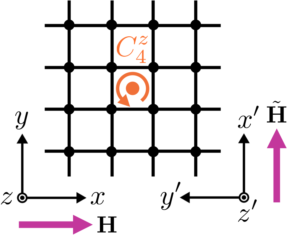
Figure 4: Example illustrating the type of symmetry constraint imposed by the Grabner–Swanson equation (Eq. 34) on systems in an external magnetic or electric field. For a square lattice with four-fold ($90^{\circ}$) rotational symmetry with respect to the $z$-axis ($C_{4}^{z}$) in the presence of an external magnetic field $\mathbf{H}$ applied along the $x$-axis, even though the magnetic field breaks the system’s $C_{4}^{z}$ symmetry, we can nevertheless use this symmetry to state that for a rank-2 field-dependent tensor $T_{ij}(\mathbf{H})$, we must have $T_{ij}(\mathbf{H})=T^{\prime}_{ij}(\tilde{\mathbf{H}})$, where $T^{\prime}_{ij}(\tilde{\mathbf{H}})$ is the tensor expressed in the transformed coordinates (passive transformation) and $\tilde{\mathbf{H}}$ is the transformed field (active transformation). For the element $T_{xz}(H\hat{\mathbf{x}})$, for example, this gives $T_{xz}(H\hat{\mathbf{x}})=T_{yz}(H\hat{\mathbf{y}})$.

IV.1 Example: Thermal Conductivity Tensor $\kappa_{ij}(\mathbf{H})$

An example of a field-dependent rank-2 tensor is the thermal conductivity tensor $\kappa_{ij}(\mathbf{H})$, given by

$$(J_{Q})_{i}=-\kappa_{ij}(\mathbf{H})\nabla_{j}T\,,$$ (37)

where $\mathbf{J}_{Q}$ is the heat current, $\boldsymbol{\nabla}T$ is the temperature gradient, and $\mathbf{H}$ is the external magnetic field. It is useful to express it as a sum of even and odd functions of the magnetic field,

$$\kappa_{ij}(\mathbf{H})=\kappa_{ij}^{\text{even}}(\mathbf{H})+\kappa_{ij}^{\text{odd}}(\mathbf{H})\,,$$ (38)

where $\kappa_{ij}^{\text{even}}(\mathbf{H})=\kappa_{ij}^{\text{even}}(-\mathbf{H})$ and $\kappa_{ij}^{\text{odd}}(\mathbf{H})=-\kappa_{ij}^{\text{odd}}(-\mathbf{H})$, and are experimentally obtained by reversing the direction of the applied field Akgoz and Saunders (1975a, b):

$$\kappa_{ij}^{\text{even}}(\mathbf{H}) =\frac{1}{2}[\kappa_{ij}(\mathbf{H})+\kappa_{ij}(-\mathbf{H})]\,,$$ (39)

$$\kappa_{ij}^{\text{odd}}(\mathbf{H}) =\frac{1}{2}[\kappa_{ij}(\mathbf{H})-\kappa_{ij}(-\mathbf{H})]\,.$$ (40)

Since $\kappa_{ij}(\mathbf{H})$ satisfies the Onsager relation Onsager (1931); Akgoz and Saunders (1975a, b)

$$\kappa_{ij}(\mathbf{H})=\kappa_{ji}(-\mathbf{H})\,,$$ (41)

then $\kappa_{ij}^{\text{even}}(\mathbf{H})$ must be a symmetric tensor and $\kappa_{ij}^{\text{odd}}(\mathbf{H})$ must be antisymmetric. In matrix form, Eq. 38 is therefore an equation of the general form

$$\kappa_{ij}(\mathbf{H})=\overset{\overset{\textbf{\small Even in $\mathbf{H}$}}{\vphantom{,}}}{\underbrace{\begin{pmatrix}A&B&C\\ B&D&E\\ C&E&F\end{pmatrix}}_{\kappa_{ij}^{\text{even}}(\mathbf{H})}}+\overset{\overset{\textbf{\small Odd in $\mathbf{H}$}}{\vphantom{,}}}{\underbrace{\begin{pmatrix}0&G&I\\ -G&0&J\\ -I&-J&0\end{pmatrix}}_{\kappa_{ij}^{\text{odd}}(\mathbf{H})}}$$ (42)

before placing any crystal symmetry constraints. Following Ref. Akgoz and Saunders (1975b), we identify $\kappa_{ij}^{\text{even}}(\mathbf{H})$ as the thermomagnetic conductivity and $\kappa_{ij}^{\text{odd}}(\mathbf{H})$ as the thermal Hall conductivity.

We will now obtain the symmetry constraints for $\kappa_{ij}(\mathbf{H})$ for the cases where the magnetic field points along a zigzag direction ($e_{1}$), an armchair direction ($e_{2}$), or the direction perpendicular to the plane ($e_{3}$). Applying the Grabner–Swanson equation (Eq. 34) using the symmetry $C_{2}^{e_{2}}$ for the case where the magnetic field points along the zigzag direction $e_{1}$ gives

$$\begin{pmatrix}\kappa_{e_{1}e_{1}}(H\hat{\mathbf{e}}_{1})&\kappa_{e_{1}e_{2}}(H\hat{\mathbf{e}}_{1})&\kappa_{e_{1}e_{3}}(H\hat{\mathbf{e}}_{1})\\ \kappa_{e_{2}e_{1}}(H\hat{\mathbf{e}}_{1})&\kappa_{e_{2}e_{2}}(H\hat{\mathbf{e}}_{1})&\kappa_{e_{2}e_{3}}(H\hat{\mathbf{e}}_{1})\\ \kappa_{e_{3}e_{1}}(H\hat{\mathbf{e}}_{1})&\kappa_{e_{3}e_{2}}(H\hat{\mathbf{e}}_{1})&\kappa_{e_{3}e_{3}}(H\hat{\mathbf{e}}_{1})\\ \vspace{-13.6pt}\hphantom{-\kappa_{e_{2}e_{1}}(-H\hat{\mathbf{e}}_{1})}&\hphantom{-\kappa_{e_{3}e_{2}}(-H\hat{\mathbf{e}}_{1})}&\hphantom{-\kappa_{e_{2}e_{3}}(-H\hat{\mathbf{e}}_{1})}\end{pmatrix}$$

$$=\begin{pmatrix}\kappa_{e_{1}e_{1}}(-H\hat{\mathbf{e}}_{1})&-\kappa_{e_{1}e_{2}}(-H\hat{\mathbf{e}}_{1})&\kappa_{e_{1}e_{3}}(-H\hat{\mathbf{e}}_{1})\\ -\kappa_{e_{2}e_{1}}(-H\hat{\mathbf{e}}_{1})&\kappa_{e_{2}e_{2}}(-H\hat{\mathbf{e}}_{1})&-\kappa_{e_{2}e_{3}}(-H\hat{\mathbf{e}}_{1})\\ \kappa_{e_{3}e_{1}}(-H\hat{\mathbf{e}}_{1})&-\kappa_{e_{3}e_{2}}(-H\hat{\mathbf{e}}_{1})&\kappa_{e_{3}e_{3}}(-H\hat{\mathbf{e}}_{1})\end{pmatrix}\,,$$ (43)

which constrains $\kappa_{ij}(H\hat{\mathbf{e}}_{1})$ to be of the form

$$\kappa_{ij}(H\hat{\mathbf{e}}_{1})=\overset{\overset{\textbf{\small Even in $H$}}{\vphantom{,}}}{\begin{pmatrix}A&0&B\\ 0&C&0\\ B&0&D\end{pmatrix}}+\overset{\overset{\textbf{\small Odd in $H$}}{\vphantom{,}}}{\begin{pmatrix}0&E&0\\ -E&0&F\\ 0&-F&0\end{pmatrix}}\,,\quad(C_{2}^{e_{2}})$$ (44)

and similarly for when the field points perpendicular to the plane (i.e., along $e_{3}$). However, if the magnetic field points along the armchair direction $e_{2}$, the Grabner–Swanson equation gives

$$\begin{pmatrix}\kappa_{e_{1}e_{1}}(H\hat{\mathbf{e}}_{2})&\kappa_{e_{1}e_{2}}(H\hat{\mathbf{e}}_{2})&\kappa_{e_{1}e_{3}}(H\hat{\mathbf{e}}_{2})\\ \kappa_{e_{2}e_{1}}(H\hat{\mathbf{e}}_{2})&\kappa_{e_{2}e_{2}}(H\hat{\mathbf{e}}_{2})&\kappa_{e_{2}e_{3}}(H\hat{\mathbf{e}}_{2})\\ \kappa_{e_{3}e_{1}}(H\hat{\mathbf{e}}_{2})&\kappa_{e_{3}e_{2}}(H\hat{\mathbf{e}}_{2})&\kappa_{e_{3}e_{3}}(H\hat{\mathbf{e}}_{2})\\ \vspace{-13.6pt}\hphantom{-\kappa_{e_{2}e_{1}}(H\hat{\mathbf{e}}_{2})}&\hphantom{-\kappa_{e_{3}e_{2}}(H\hat{\mathbf{e}}_{2})}&\hphantom{-\kappa_{e_{2}e_{3}}(H\hat{\mathbf{e}}_{2})}\end{pmatrix}$$

$$=\begin{pmatrix}\kappa_{e_{1}e_{1}}(H\hat{\mathbf{e}}_{2})&-\kappa_{e_{1}e_{2}}(H\hat{\mathbf{e}}_{2})&\kappa_{e_{1}e_{3}}(H\hat{\mathbf{e}}_{2})\\ -\kappa_{e_{2}e_{1}}(H\hat{\mathbf{e}}_{2})&\kappa_{e_{2}e_{2}}(H\hat{\mathbf{e}}_{2})&-\kappa_{e_{2}e_{3}}(H\hat{\mathbf{e}}_{2})\\ \kappa_{e_{3}e_{1}}(H\hat{\mathbf{e}}_{2})&-\kappa_{e_{3}e_{2}}(H\hat{\mathbf{e}}_{2})&\kappa_{e_{3}e_{3}}(H\hat{\mathbf{e}}_{2})\end{pmatrix}\,,$$ (45)

which constrains $\kappa_{ij}(H\hat{\mathbf{e}}_{2})$ to be of the form

$$\kappa_{ij}(H\hat{\mathbf{e}}_{2})=\overset{\overset{\textbf{\small Even in $H$}}{\vphantom{,}}}{\begin{pmatrix}G&0&I\\ 0&J&0\\ I&0&K\end{pmatrix}}+\overset{\overset{\textbf{\small Odd in $H$}}{\vphantom{,}}}{\begin{pmatrix}0&0&L\\ 0&0&0\\ -L&0&0\\ \vspace{-13.6pt}\hphantom{-Q}&\hphantom{-R}&\hphantom{R}\end{pmatrix}}\,.\quad(C_{2}^{e_{2}})$$ (46)

The symmetry $C_{3}^{e_{3}}$ does not constrain the form of $\kappa_{ij}(\mathbf{H})$ when the magnetic field points along the zigzag or armchair directions $e_{1}$ and $e_{2}$. This is because when $\mathbf{H}$ points along the zigzag direction $e_{1}$, the Grabner–Swanson equation gives $\kappa_{ij}(H\hat{\mathbf{e}}_{1})=\kappa^{\prime}_{ij}\bigl{(}H(-\tfrac{1}{2}\hat{\mathbf{e}}_{1}+\tfrac{\sqrt{3}}{2}\hat{\mathbf{e}}_{2})\bigr{)}$, which is not a useful constraint because the field on the right side of the equation does not point along any of the three high-symmetry axes that we are interested in (i.e., $e_{1},e_{2},e_{3}$), and similarly for when $\mathbf{H}$ points along the armchair direction $e_{2}$. However, for the case where the magnetic field points perpendicular to the plane ($e_{3}$ direction), $C_{3}^{e_{3}}$ imposes the same constraints as for the field-independent case (see Eq. 16), so $\kappa_{ij}(H\hat{\mathbf{e}}_{3})$ is of the form

$$\kappa_{ij}(H\hat{\mathbf{e}}_{3})=\begin{pmatrix}A&B&0\\ -B&A&0\\ 0&0&C\end{pmatrix}\,.\qquad(C_{3}^{e_{3}})$$ (47)

Identifying the symmetric and antisymmetric terms as even and odd functions of $H$, respectively, gives

$$\kappa_{ij}(H\hat{\mathbf{e}}_{3})=\overset{\overset{\textbf{\small Even in $H$}}{\vphantom{,}}}{\begin{pmatrix}A&0&0\\ 0&A&0\\ 0&0&C\end{pmatrix}}+\overset{\overset{\textbf{\small Odd in $H$}}{\vphantom{,}}}{\begin{pmatrix}0&B&0\\ -B&0&0\\ 0&0&0\end{pmatrix}}\,.\quad(C_{3}^{e_{3}})$$ (48)

Finally, inversion symmetry does not impose any constraints on $\kappa_{ij}(\mathbf{H})$, since $\mathbf{H}$ is not affected by inversion, and $\mathbf{J}_{Q}$ and $\boldsymbol{\nabla}T$ both change sign under inversion, which leaves $\kappa_{ij}$ unchanged.

The most general forms of the magnetic-field-dependent thermal conductivity tensor $\kappa_{ij}(\mathbf{H})$ for the eight point groups generated by these three symmetries (see Table 1) are given in Table 3. As an example, for a material of the monoclinic point group $2/m$ in an external magnetic field $\mathbf{H}$ along the zigzag axis $e_{1}$, the thermal Hall conductivity corresponding to a heat current $\mathbf{J}_{Q}$ along $e_{1}$ and a temperature gradient $\boldsymbol{\nabla}T$ along the armchair axis $e_{2}$ is given by the following boxed entry in Table 3:

$$2,~{}2/m:~{}\kappa_{ij}(H\hat{\mathbf{e}}_{1})=\overset{\overset{\textbf{\small Even in $H$}}{\vphantom{,}}}{\begin{pmatrix}A&0&B\\ 0&C&0\\ B&0&D\end{pmatrix}}+\overset{\overset{\textbf{\small Odd in $H$}}{\vphantom{,}}}{\begin{pmatrix}\cline{2-2}\cr 0&\vrule\lx@intercol\hfil E\hfil\lx@intercol\vrule\lx@intercol&0\\ \cline{2-2}\cr-E&0&F\\ 0&-F&0\\ \vspace{-13.6pt}\hphantom{-G_{3}}&\hphantom{-J_{3}}&\hphantom{-J_{3}}\end{pmatrix}.}$$ (49)

Similarly to the thermomagnetic susceptibility tensor discussed in Section III.2, even if components such as $\kappa_{e_{3}e_{1}}(\mathbf{H})$ and $\kappa_{e_{1}e_{3}}(\mathbf{H})$ are allowed by symmetry for a given point group and field orientation, we expect them to be zero for monolayer or few-layer systems.

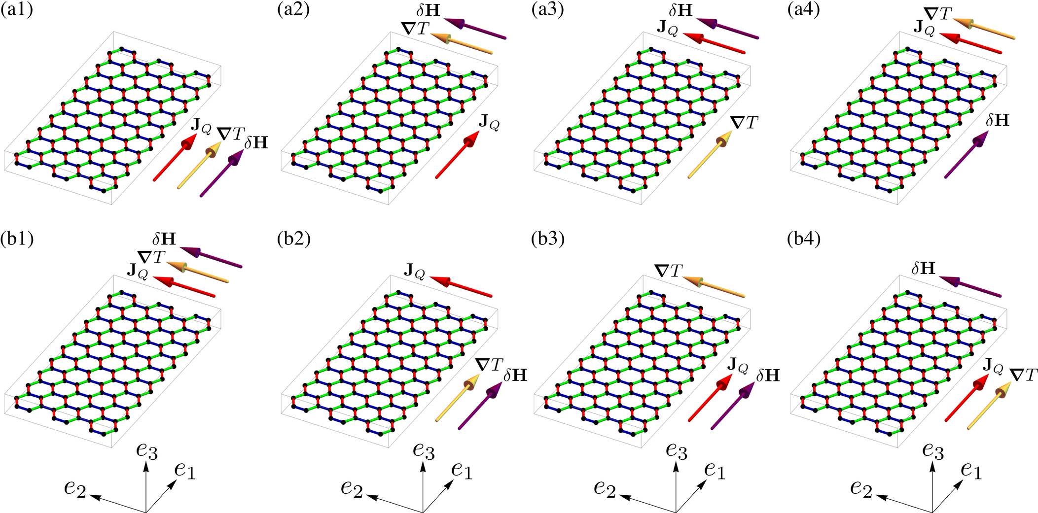
Figure 5: Illustration of the two sets of unusual equalities (Eqs. 23 and 24) for zero-field rank-3 tensors describing crystals with $C_{3}^{e_{3}}$ symmetry (i.e., belonging to the trigonal point groups $3$, $\bar{3}$, $32$, or $\bar{3}m$). The changes in the thermal conductivity that results from applying a small magnetic field $\delta\mathbf{H}$ in scenarios (a1)–(a4) all have the same magnitude, i.e. $|\delta\kappa_{e_{1}e_{1}}(\delta\mathbf{H}\parallel\hat{\mathbf{e}}_{1})|=|\delta\kappa_{e_{1}e_{2}}(\delta\mathbf{H}\parallel\hat{\mathbf{e}}_{2})|=|\delta\kappa_{e_{2}e_{1}}(\delta\mathbf{H}\parallel\hat{\mathbf{e}}_{2})|=|\delta\kappa_{e_{2}e_{2}}(\delta\mathbf{H}\parallel\hat{\mathbf{e}}_{1})|$, and similarly for scenarios (b1)–(b4). Reversing the direction of any one of these vectors simply reverses the sign of the change in the thermal conductivity. These results hold when the system is either not magnetized, or magnetized along the out-of-plane direction ($e_{3}$). Even though these illustrations describe the thermomagnetic susceptibility tensor $\chi^{\text{thermomag}}_{ijk}=(\partial\kappa_{ij}/\partial H_{k})|_{\mathbf{H}=\mathbf{0}}$ for concreteness, they more generally apply to any general rank-3 tensor describing a system in the absence of external magnetic or electric fields by simply replacing the heat current $\mathbf{J}_{Q}$, temperature gradient $\boldsymbol{\nabla}T$, and small magnetic field $\delta\mathbf{H}$ with any three vector quantities as long as they are not large external fields (however, small magnetic or electric fields that are used to probe the system, i.e. $\delta\mathbf{H}$ and $\delta\mathbf{E}$, are allowed).

V Summary of Predictions for Experiments

In this section we discuss the main predictions from our symmetry analysis and compare some of them with recent experiments.

V.1 Predictions for Zero-Field Tensors

We obtained the most general forms of rank-2 and rank-3 tensors expressed in the $e_{1}e_{2}e_{3}$ coordinates ($e_{1}$ = zigzag direction, $e_{2}$ = armchair direction, $e_{3}$ = out-of-plane direction; see Fig. 1) for crystals of various point groups in the absence of an external field. These results are listed in Table 3. We now highlight some notable predictions for these zero-field tensors for crystals of various point groups.

For systems with $C_{3}^{e_{3}}$ symmetry (i.e., crystals belonging to the trigonal point groups $3$, $\bar{3}$, $32$, or $\bar{3}m$ that are either not magnetized or magnetized along the out-of-plane direction) in the absence of an external field:

• Rank-3 tensors have several unusual equalities between fully longitudinal and partly transverse in-plane components, as illustrated in Fig. 5 using the thermomagnetic susceptibility tensor $\chi^{\text{thermomag}}_{ijk}=(\partial\kappa_{ij}/\partial H_{k})|_{\mathbf{H}=\mathbf{0}}$ (where $\kappa_{ij}$ is the thermal conductivity tensor) for concreteness.

• Rank-2 tensors have continuous rotational symmetry with respect to the axis perpendicular to the plane, so rank-2 responses (e.g., magnetic susceptibility $\chi_{ij}=(\partial M_{i}/\partial H_{j})|_{\mathbf{H}=\mathbf{0}}$) behave the same way along all in-plane directions, including low-symmetry directions.

For systems with $C_{2}^{e_{2}}$ symmetry (i.e., crystals belonging to the monoclinic point groups $2$ or $2/m$, or to the trigonal point groups $32$, or $\bar{3}m$ that are either not magnetized or magnetized along an axis that does not have $C_{2}$ symmetry) in the absence of an external field:

• For tensors of all ranks, all tensor components corresponding to an odd number of $e_{1}+e_{3}$ directions are zero; for example, the following magnetic susceptibilities are zero: $\chi_{e_{1}e_{2}}$, $\chi_{e_{2}e_{1}}$, $\chi_{e_{3}e_{2}}$, $\chi_{e_{2}e_{3}}$.

V.2 Predictions for the Thermal Conductivity Tensor $\kappa_{ij}(\mathbf{H})$

We also obtained the most general forms of the thermal conductivity tensor $\kappa_{ij}(\mathbf{H})$ for crystals of various point groups in an external magnetic field along the high-symmetry directions $e_{1}$, $e_{2}$, and $e_{3}$ ($e_{1}$ = zigzag direction, $e_{2}$ = armchair direction, $e_{3}$ = out-of-plane direction;). We looked at the components of $\kappa_{ij}(\mathbf{H})$ that are even and odd functions of the magnetic field $\mathbf{H}$ separately, where the even terms correspond to the thermomagnetic conductivity and the odd terms correspond to the thermal Hall conductivity. These results are also listed in Table 3. We now highlight some notable predictions for the thermal conductivity tensor for crystals of various point groups.

For crystals with $C_{3}^{e_{3}}$ symmetry (i.e., belonging to the trigonal point groups $3$, $\bar{3}$, $32$, or $\bar{3}m$) in an external magnetic field:

• When $\mathbf{H}$ points perpendicular to the plane (i.e., along $e_{3}$), $\kappa_{ij}(\mathbf{H})$ has continuous rotational symmetry with respect to this axis, so the thermal conductivity and thermal Hall conductivity behave the same way along all in-plane directions, including low-symmetry directions.

For crystals with $C_{2}^{e_{2}}$ symmetry (i.e., belonging to the monoclinic point groups $2$ or $2/m$, or to the trigonal point groups $32$, or $\bar{3}m$) in an external magnetic field:

• In an external magnetic field $\mathbf{H}$ along the in-plane zigzag axis $e_{1}$, applying a heat current $\mathbf{J}_{Q}$ along $e_{1}$ can produce a thermal Hall response (i.e., a transverse temperature gradient $\boldsymbol{\nabla}T$ along the high-symmetry armchair axis $e_{2}$ that reverses direction upon reversing the direction of $\mathbf{H}$). This has been observed in a recent thermal Hall experiment on $\alpha$-RuCl₃ (belonging to the monoclinic point group $2/m$ Johnson et al. (2015)) by Yokoi et al. Yokoi et al. (2020) (see Fig. 3a with $\delta\mathbf{H}$ replaced by $\mathbf{H}$ for an illustration of the orientations used in this experiment), as well as corroborated analytically and numerically by Chern, Zhang, & Kim Chern et al. (2020); Zhang et al. (2021).

• When $\mathbf{H}$ is along the in-plane high-symmetry armchair axis $e_{2}$, applying a heat current $\mathbf{J}_{Q}$ along the zigzag axis also $e_{1}$ cannot produce a thermal Hall response (i.e., a transverse temperature gradient $\boldsymbol{\nabla}T$ along $e_{2}$ that reverses direction upon reversing the direction of $\mathbf{H}$). This was also observed in $\alpha$-RuCl₃ by Yokoi et al. Yokoi et al. (2020) and corroborated analytically and numerically by Chern et al. Chern et al. (2020); Zhang et al. (2021).

• When $\mathbf{H}$ is along the in-plane high-symmetry armchair axis $e_{2}$, applying a heat current $\mathbf{J}_{Q}$ along $e_{2}$ cannot produce a thermal Hall response (i.e., a transverse temperature gradient $\boldsymbol{\nabla}T$ along the zigzag axis $e_{1}$ that reverses direction upon reversing the direction of $\mathbf{H}$). Relative to the orientations described in the first bullet point, this corresponds to interchanging which vectors point along $e_{1}$ and $e_{2}$ (i.e., $e_{1}\leftrightarrow e_{2}$), or equivalently, to rotating the three vectors by $90^{\circ}$ with respect to the out-of-plane axis.

Other experiments have also observed a thermal Hall effect in $\alpha$-RuCl₃ when the magnetic field is applied in the plane, although the direction of the field within the plane was not known Hentrich et al. (2018, 2019, 2020). More experiments are needed to get a better understanding of the tensorial character of the thermal Hall response in these materials.

VI Outlook

This work has the potential to guide future experiments seeking to probe new physical responses along different geometries in 2D materials, similarly to the unusual thermal Hall effect observed in $\alpha$-RuCl₃ when the magnetic field is applied in the plane Yokoi et al. (2020). Our analysis can also help inform the search for existing 2D materials or the design of novel materials having specific desirable properties (e.g., the presence or absence of a given longitudinal or transverse physical response). Finally, this analysis can aid in the identification of the crystal structure (specifically, the point group) of new 2D materials. The analysis presented here can also be extended to the magnetic point group symmetries following a similar procedure.

VII Acknowledgments

We thank Joshua E. Goldberger for useful discussions about crystal symmetries and point groups in these 2D systems. We also thank Joseph P. Heremans and Rolando Valdés Aguilar for their helpful feedback and for pointing us to various relevant references. Finally, we thank Brian Skinner, Zachariah Addison, Joseph Szabo, Humberto Gilmer, and Daniella Roberts for their feedback. This research was partially supported by the Center of Emergent Materials, an NSF MRSEC under award number DMR-2011876, and from BES-DOE grant DE-FG02-07ER46423.

References

- Zhang et al. (2015) W.-B. Zhang, Q. Qu, P. Zhu, and C.-H. Lam, J. Mater. Chem. C 3, 12457 (2015).
- Huang et al. (2017) B. Huang, G. Clark, E. Navarro-Moratalla, D. R. Klein, R. Cheng, K. L. Seyler, D. Zhong, E. Schmidgall, M. A. McGuire, D. H. Cobden, W. Yao, D. Xiao, P. Jarillo-Herrero, and X. Xu, Nature 546, 270 (2017).
- Gong et al. (2017) C. Gong, L. Li, Z. Li, H. Ji, A. Stern, Y. Xia, T. Cao, W. Bao, C. Wang, Y. Wang, Z. Q. Qiu, R. J. Cava, S. G. Louie, J. Xia, and X. Zhang, Nature 546, 265 (2017).
- Burch et al. (2018) K. S. Burch, D. Mandrus, and J.-G. Park, Nature 563, 47 (2018).
- Lado and Fernández-Rossier (2017) J. L. Lado and J. Fernández-Rossier, 2D Materials 4, 035002 (2017).
- Huang et al. (2018) B. Huang, G. Clark, D. R. Klein, D. MacNeill, E. Navarro-Moratalla, K. L. Seyler, N. Wilson, M. A. McGuire, D. H. Cobden, D. Xiao, W. Yao, P. Jarillo-Herrero, and X. Xu, Nature Nanotechnology 13, 544 (2018).
- Jiang et al. (2018a) S. Jiang, L. Li, Z. Wang, K. F. Mak, and J. Shan, Nature Nanotechnology 13, 549 (2018a).
- Wang et al. (2018) Z. Wang, I. Gutiérrez-Lezama, N. Ubrig, M. Kroner, M. Gibertini, T. Taniguchi, K. Watanabe, A. Imamoğlu, E. Giannini, and A. F. Morpurgo, Nature Communications 9, 2516 (2018).
- Liu et al. (2018) J. Liu, M. Shi, P. Mo, and J. Lu, AIP Advances 8, 055316 (2018).
- Chen et al. (2018) L. Chen, J.-H. Chung, B. Gao, T. Chen, M. B. Stone, A. I. Kolesnikov, Q. Huang, and P. Dai, Phys. Rev. X 8, 041028 (2018).
- Lee et al. (2020) I. Lee, F. G. Utermohlen, D. Weber, K. Hwang, C. Zhang, J. van Tol, J. E. Goldberger, N. Trivedi, and P. C. Hammel, Phys. Rev. Lett. 124, 017201 (2020).
- Chen et al. (2020) L. Chen, J.-H. Chung, T. Chen, C. Duan, A. Schneidewind, I. Radelytskyi, D. J. Voneshen, R. A. Ewings, M. B. Stone, A. I. Kolesnikov, B. Winn, S. Chi, R. A. Mole, D. H. Yu, B. Gao, and P. Dai, Phys. Rev. B 101, 134418 (2020).
- McCreary et al. (2020) A. McCreary, T. T. Mai, F. G. Utermohlen, J. R. Simpson, K. F. Garrity, X. Feng, D. Shcherbakov, Y. Zhu, J. Hu, D. Weber, K. Watanabe, T. Taniguchi, J. E. Goldberger, Z. Mao, C. N. Lau, Y. Lu, N. Trivedi, R. Valdés Aguilar, and A. R. Hight Walker, Nature Communications 11, 3879 (2020).
- Soriano et al. (2020) D. Soriano, M. I. Katsnelson, and J. Fernández-Rossier, Nano Letters 20, 6225 (2020), pMID: 32787171.
- Kitaev (2006) A. Kitaev, Annals of Physics 321, 2 (2006), January Special Issue.
- Jackeli and Khaliullin (2009) G. Jackeli and G. Khaliullin, Phys. Rev. Lett. 102, 017205 (2009).
- Chaloupka et al. (2010) J. Chaloupka, G. Jackeli, and G. Khaliullin, Phys. Rev. Lett. 105, 027204 (2010).
- Rau et al. (2014) J. G. Rau, E. K.-H. Lee, and H.-Y. Kee, Phys. Rev. Lett. 112, 077204 (2014).
- Banerjee et al. (2016) A. Banerjee, C. A. Bridges, J. Q. Yan, A. A. Aczel, L. Li, M. B. Stone, G. E. Granroth, M. D. Lumsden, Y. Yiu, J. Knolle, S. Bhattacharjee, D. L. Kovrizhin, R. Moessner, D. A. Tennant, D. G. Mandrus, and S. E. Nagler, Nature Materials 15, 733 (2016).
- Banerjee et al. (2017) A. Banerjee, J. Yan, J. Knolle, C. A. Bridges, M. B. Stone, M. D. Lumsden, D. G. Mandrus, D. A. Tennant, R. Moessner, and S. E. Nagler, Science 356, 1055 (2017).
- Baek et al. (2017) S.-H. Baek, S.-H. Do, K.-Y. Choi, Y. S. Kwon, A. U. B. Wolter, S. Nishimoto, J. van den Brink, and B. Büchner, Phys. Rev. Lett. 119, 037201 (2017).
- Banerjee et al. (2018) A. Banerjee, P. Lampen-Kelley, J. Knolle, C. Balz, A. A. Aczel, B. Winn, Y. Liu, D. Pajerowski, J. Yan, C. A. Bridges, A. T. Savici, B. C. Chakoumakos, M. D. Lumsden, D. A. Tennant, R. Moessner, D. G. Mandrus, and S. E. Nagler, npj Quantum Materials 3, 8 (2018).
- Takagi et al. (2019) H. Takagi, T. Takayama, G. Jackeli, G. Khaliullin, and S. E. Nagler, Nature Reviews Physics 1, 264 (2019).
- Kane and Mele (2005) C. L. Kane and E. J. Mele, Phys. Rev. Lett. 95, 146802 (2005).
- Hasan and Kane (2010) M. Z. Hasan and C. L. Kane, Rev. Mod. Phys. 82, 3045 (2010).
- Lu and Vishwanath (2012) Y.-M. Lu and A. Vishwanath, Phys. Rev. B 86, 125119 (2012).
- Owerre (2016) S. A. Owerre, Journal of Physics: Condensed Matter 28, 386001 (2016).
- Kou et al. (2017) L. Kou, Y. Ma, Z. Sun, T. Heine, and C. Chen, The Journal of Physical Chemistry Letters 8, 1905 (2017).
- Pershoguba et al. (2018) S. S. Pershoguba, S. Banerjee, J. C. Lashley, J. Park, H. Ågren, G. Aeppli, and A. V. Balatsky, Phys. Rev. X 8, 011010 (2018).
- McClarty et al. (2018) P. A. McClarty, X.-Y. Dong, M. Gohlke, J. G. Rau, F. Pollmann, R. Moessner, and K. Penc, Phys. Rev. B 98, 060404(R) (2018).
- Plumb et al. (2014) K. W. Plumb, J. P. Clancy, L. J. Sandilands, V. V. Shankar, Y. F. Hu, K. S. Burch, H.-Y. Kee, and Y.-J. Kim, Phys. Rev. B 90, 041112(R) (2014).
- Sears et al. (2015) J. A. Sears, M. Songvilay, K. W. Plumb, J. P. Clancy, Y. Qiu, Y. Zhao, D. Parshall, and Y.-J. Kim, Phys. Rev. B 91, 144420 (2015).
- Kasahara et al. (2018a) Y. Kasahara, T. Ohnishi, Y. Mizukami, O. Tanaka, S. Ma, K. Sugii, N. Kurita, H. Tanaka, J. Nasu, Y. Motome, T. Shibauchi, and Y. Matsuda, Nature 559, 227 (2018a).
- Yokoi et al. (2020) T. Yokoi, S. Ma, Y. Kasahara, S. Kasahara, T. Shibauchi, N. Kurita, H. Tanaka, J. Nasu, Y. Motome, C. Hickey, S. Trebst, and Y. Matsuda, (2020), arXiv:2001.01899 [cond-mat.str-el] .
- Janssen and Vojta (2019) L. Janssen and M. Vojta, Journal of Physics: Condensed Matter 31, 423002 (2019).
- Hickey and Trebst (2019) C. Hickey and S. Trebst, Nature Communications 10, 530 (2019).
- Ronquillo et al. (2019) D. C. Ronquillo, A. Vengal, and N. Trivedi, Phys. Rev. B 99, 140413(R) (2019).
- Hickey et al. (2021) C. Hickey, M. Gohlke, C. Berke, and S. Trebst, Phys. Rev. B 103, 064417 (2021).
- Gohlke et al. (2018) M. Gohlke, R. Moessner, and F. Pollmann, Phys. Rev. B 98, 014418 (2018).
- Gordon et al. (2019) J. S. Gordon, A. Catuneanu, E. S. Sørensen, and H.-Y. Kee, Nature Communications 10, 2470 (2019).
- Patel and Trivedi (2019) N. D. Patel and N. Trivedi, Proceedings of the National Academy of Sciences 116, 12199 (2019).
- Nasu and Motome (2019) J. Nasu and Y. Motome, Phys. Rev. Research 1, 033007 (2019).
- Pradhan et al. (2020) S. Pradhan, N. D. Patel, and N. Trivedi, Phys. Rev. B 101, 180401(R) (2020).
- Jiang et al. (2018b) H.-C. Jiang, C.-Y. Wang, B. Huang, and Y.-M. Lu, (2018b), arXiv:1809.08247 [cond-mat.str-el] .
- Ozel et al. (2019) I. O. Ozel, C. A. Belvin, E. Baldini, I. Kimchi, S. Do, K.-Y. Choi, and N. Gedik, Phys. Rev. B 100, 085108 (2019).
- McGuire (2017) M. A. McGuire, Crystals 7, 121 (2017).
- Winter et al. (2017) S. M. Winter, A. A. Tsirlin, M. Daghofer, J. van den Brink, Y. Singh, P. Gegenwart, and R. Valentí, Journal of Physics: Condensed Matter 29, 493002 (2017).
- Trebst (2017) S. Trebst, (2017), arXiv:1701.07056 [cond-mat.str-el] .
- O’Malley et al. (2008) M. J. O’Malley, H. Verweij, and P. M. Woodward, Journal of Solid State Chemistry 181, 1803 (2008).
- Choi et al. (2012) S. K. Choi, R. Coldea, A. N. Kolmogorov, T. Lancaster, I. I. Mazin, S. J. Blundell, P. G. Radaelli, Y. Singh, P. Gegenwart, K. R. Choi, S.-W. Cheong, P. J. Baker, C. Stock, and J. Taylor, Phys. Rev. Lett. 108, 127204 (2012).
- Singh et al. (2012) Y. Singh, S. Manni, J. Reuther, T. Berlijn, R. Thomale, W. Ku, S. Trebst, and P. Gegenwart, Phys. Rev. Lett. 108, 127203 (2012).
- Hwan Chun et al. (2015) S. Hwan Chun, J.-W. Kim, J. Kim, H. Zheng, C. C. Stoumpos, C. D. Malliakas, J. F. Mitchell, K. Mehlawat, Y. Singh, Y. Choi, T. Gog, A. Al-Zein, M. M. Sala, M. Krisch, J. Chaloupka, G. Jackeli, G. Khaliullin, and B. J. Kim, Nature Physics 11, 462 (2015).
- Winter et al. (2016) S. M. Winter, Y. Li, H. O. Jeschke, and R. Valentí, Phys. Rev. B 93, 214431 (2016).
- Birss (1964) R. Birss, Symmetry and Magnetism, Selected topics in solid state physics (North-Holland Publishing Company, 1964).
- Post (1978) E. J. Post, Foundations of Physics 8, 277 (1978).
- Shapiro et al. (2015) M. C. Shapiro, P. Hlobil, A. T. Hristov, A. V. Maharaj, and I. R. Fisher, Phys. Rev. B 92, 235147 (2015).
- Sorensen and Fisher (2020) M. E. Sorensen and I. R. Fisher, (2020), arXiv:2009.01975 [cond-mat.str-el] .
- Akgoz and Saunders (1975a) Y. C. Akgoz and G. A. Saunders, Journal of Physics C: Solid State Physics 8, 1387 (1975a).
- Hentrich et al. (2020) R. Hentrich, X. Hong, M. Gillig, F. Caglieris, M. Čulo, M. Shahrokhvand, U. Zeitler, M. Roslova, A. Isaeva, T. Doert, L. Janssen, M. Vojta, B. Büchner, and C. Hess, Phys. Rev. B 102, 235155 (2020).
- Hentrich et al. (2019) R. Hentrich, M. Roslova, A. Isaeva, T. Doert, W. Brenig, B. Büchner, and C. Hess, Phys. Rev. B 99, 085136 (2019).
- Kasahara et al. (2018b) Y. Kasahara, K. Sugii, T. Ohnishi, M. Shimozawa, M. Yamashita, N. Kurita, H. Tanaka, J. Nasu, Y. Motome, T. Shibauchi, and Y. Matsuda, Phys. Rev. Lett. 120, 217205 (2018b).
- Hentrich et al. (2018) R. Hentrich, A. U. B. Wolter, X. Zotos, W. Brenig, D. Nowak, A. Isaeva, T. Doert, A. Banerjee, P. Lampen-Kelley, D. G. Mandrus, S. E. Nagler, J. Sears, Y.-J. Kim, B. Büchner, and C. Hess, Phys. Rev. Lett. 120, 117204 (2018).
- Note (1) The choice of which three point group symmetries we use as the generating symmetries is not unique; they just have to be linearly independent. For example, we could have used a mirror symmetry instead of the inversion symmetry.
- Johnson et al. (2015) R. D. Johnson, S. C. Williams, A. A. Haghighirad, J. Singleton, V. Zapf, P. Manuel, I. I. Mazin, Y. Li, H. O. Jeschke, R. Valentí, and R. Coldea, Phys. Rev. B 92, 235119 (2015).
- McGuire et al. (2015) M. A. McGuire, H. Dixit, V. R. Cooper, and B. C. Sales, Chemistry of Materials 27, 612 (2015).
- McGuire et al. (2017) M. A. McGuire, G. Clark, K. C. Santosh, W. M. Chance, G. E. Jellison, V. R. Cooper, X. Xu, and B. C. Sales, Phys. Rev. Materials 1, 014001 (2017).
- Lee et al. (2016) J.-U. Lee, S. Lee, J. H. Ryoo, S. Kang, T. Y. Kim, P. Kim, C.-H. Park, J.-G. Park, and H. Cheong, Nano Letters 16, 7433 (2016).
- Ubrig et al. (2020) N. Ubrig, Z. Wang, J. Teyssier, T. Taniguchi, K. Watanabe, E. Giannini, A. F. Morpurgo, and M. Gibertini, 2D Materials 7, 015007 (2020).
- Kong et al. (2019) T. Kong, K. Stolze, E. I. Timmons, J. Tao, D. Ni, S. Guo, Z. Yang, R. Prozorov, and R. J. Cava, Advanced Materials 31, 1808074 (2019).
- Doležal et al. (2019) P. Doležal, M. Kratochvílová, V. Holý, P. Čermák, V. Sechovský, M. Dušek, M. Míšek, T. Chakraborty, Y. Noda, S. Son, and J.-G. Park, Phys. Rev. Materials 3, 121401(R) (2019).
- Carteaux et al. (1995) V. Carteaux, D. Brunet, G. Ouvrard, and G. Andre, Journal of Physics: Condensed Matter 7, 69 (1995).
- Wiedenmann et al. (1981) A. Wiedenmann, J. Rossat-Mignod, A. Louisy, R. Brec, and J. Rouxel, Solid State Communications 40, 1067 (1981).
- Note (2) We are using the Einstein summation convention for repeated indices throughout this paper.
- Andrade et al. (2020) E. C. Andrade, L. Janssen, and M. Vojta, Phys. Rev. B 102, 115160 (2020).
- Shivaram (2014) B. S. Shivaram, Review of Scientific Instruments 85, 046107 (2014).
- Shivaram et al. (2014) B. S. Shivaram, D. G. Hinks, M. B. Maple, M. A. deAndrade, and P. Kumar, Phys. Rev. B 89, 241107(R) (2014).
- Shivaram et al. (2017) B. S. Shivaram, E. Colineau, J. Griveau, P. Kumar, and V. Celli, Journal of Physics: Condensed Matter 29, 095805 (2017).
- Shivaram et al. (2018) B. S. Shivaram, J. Luo, G.-W. Chern, D. Phelan, R. Fittipaldi, and A. Vecchione, Phys. Rev. B 97, 100403(R) (2018).
- Note (3) Of course, the component can still be nonzero in monolayer systems, since the magnetic field can be oriented perpendicular to the honeycomb plane, as is commonly the case thermal Hall experiments Kasahara et al. (2018a).
- Note (4) For example, for the rank-3 tensor component , and .
- Note (5) Throughout this paper, we will assume that each tensor index transforms as either a polar vector or an axial vector. We will therefore not consider tensors of the form for polar and axial, for example, as these are just linear combinations of the types of tensors we will consider.
- Grabner and Swanson (1962) L. Grabner and J. A. Swanson, Journal of Mathematical Physics 3, 1050 (1962).
- Akgoz and Saunders (1975b) Y. C. Akgoz and G. A. Saunders, Journal of Physics C: Solid State Physics 8, 2962 (1975b).
- Note (6) For systems with more than one external field (, , ), the Grabner–Swanson equation (Eq. 34) generalizes to ).
- Onsager (1931) L. Onsager, Phys. Rev. 37, 405 (1931).
- Chern et al. (2020) L. E. Chern, E. Z. Zhang, and Y. B. Kim, (2020), arXiv:2008.12788 [cond-mat.str-el] .
- Zhang et al. (2021) E. Z. Zhang, L. E. Chern, and Y. B. Kim, (2021), arXiv:2102.00014 [cond-mat.str-el] .