Solar System, Astrophysics, and Cosmology from the Derivative Expansion

Nidal Haddad¹ and Fateen Haddad^2
1Department of Physics, Bethlehem University
P.O.Box 9, Bethlehem, Palestine

haddad.nidal02@gmail.com, f.a.assaleh@gmail.com

Abstract

In this paper we show how the solar system, the galactic, and the cosmological scales, are accommodated in a single framework, namely, in the derivative expansion framework. We construct a locally inertial static metric, based on the Einstein equations and on the derivative expansion method, which describes a Schwarzschild black hole immersed in dark matter and dark energy. The leading order metric in the expansion corresponds to the solar system, the first order metric to the galaxy, and the second order metric to cosmology. It is shown how this metric captures the main observations at each scale: in the solar system it trivially gives the Keplerian physics, in the galaxy it gives the flat part of the rotation curve and the Baryonic Tully-Fisher relation, and in the cosmological scale it gives the cosmological redshift, the accelerating expansion, and it coincides with the Robertson-Walker spacetime in the appropriate limit and approximation.

1 Introduction

The fact that a general coordinate transformation does not change the physics in General Relativity (the principle of general covariance) does not mean that all coordinate systems are of the same importance and relevance to our observations of the universe. After all, we are locally inertial observers of the universe (the principle of equivalence) and therefore using a locally inertial coordinate system would be the most appropriate for our observations. The Schwarzschild metric in the standard form is one fundamental solution of the Einstein equations that is written in locally inertial coordinates; the locally inertial observer is sitting far away from the spherical gravitational source (e.g., a star, a black hole, etc.) where the metric is approximately Minkowski. The Schwarzschild metric is the basis for the classical tests of General Relativity, and it is especially successful when applied to planetary motions about the Sun. This metric describes, however, an isolated source (from the rest of the universe) as the asymptotes are flat. On the other hand, the Friedmann–Lemaître–Robertson–Walker metric (in short FLRW) is another fundamental solution of the Einstein equations which describes the large scale structure of the universe such as the cosmological redshift and the accelerating expansion, but it is written in global coordinates and not in locally inertial ones. The search for a locally inertial metric that accommodates both the local observations (the physics around a nearby spherical source, given by the Schwarzschild metric) and the cosmological observations (given by the FLRW spacetime) is not new, but almost as old as General Relativity is (see for example [1, 2, 3, 4, 5, 6] and the references therein).

In this paper we introduce a new approach for solving this problem, based on the derivative expansion method applied to the Einstein equations. The idea is to take the Schwarzschild black hole as the seed metric that describes the local physics and build over it a more general metric describing a black hole immersed in dark matter and dark energy (being the main constituents of the universe). To observe the effects of dark matter and dark energy large distances are required from the point of view of the locally inertial observer, and similarly, significant changes in the cosmos due to dark matter and dark energy require large distances as well with respect to this observer. Thus, the contributions of dark matter and dark energy to our (locally inertial) metric seem to accept being expanded in derivatives; that is, the derivatives of those contributions to the metric seem to be very small compared to the local scales. We argue in this paper that the metric up to second order in derivatives is static and we show that: (1) The leading (zeroth) order metric in the expansion is the Schwarzschild metric corresponding to the solar system scale, (2) The first order metric corresponds to the galactic scale (the physics due to dark matter), as it gives the main features of the rotation curve of galaxies, like the flat part and the Baryonic Tully-Fisher relation [15, 16, 17], and (3) The second order metric corresponds to the cosmological scale (the physics due to dark energy) and it is shown to coincide with the FLRW spacetime in the appropriate limit and approximation, and it gives rise to the cosmological redshift and the accelerating expansion.

The intermediate scale (the galactic scale) was missed in the previous attempts at attacking this problem (in the references [1, 2, 3, 4, 5, 6] and subsequent works), whereas in this paper it is shown to be an important matching region between the solar system and cosmological scale. In this sense, one of the main results of this paper is to put the three fundamental scales (solar system, galactic, and cosmological) consistently in a single framework; in the derivative expansion framework.

An interesting result of this analysis is to show, qualitatively and quantitatively, from the locally inertial metric found in this paper, how the anisotropies in space die out as we move up from the galactic scale to the cosmological one, where the metric goes to the FLRW spacetime in the cosmological limit. Relatedly, the energy-momentum tensor of dark matter and dark energy sourcing this spacetime is found, with a nontrivial and interesting $r$-dependence, that is, it encodes information about dark matter and dark energy at all distances. The energy-momentum tensor is that of an anisotropic fluid and it is shown to reduce to an isotropic fluid in the cosmological limit.

The paper is organised as follows. In Sec.[2] we introduce the derivative expansion method and apply it to build our locally inertial metric up to second order in derivatives. The leading order terms of the metric are shown to correspond to the solar system, the first order terms to astrophysics of galaxies, and the second order terms to cosmology. In Sec.[3] we show how the derivative expansion method is applied to the FLRW metric and how it reduces to a static local form if we change coordinates and perform the expansion up to second order in derivatives. In Sec.[4] we show how the cosmological redshift is calculated from the locally inertial static metric. Sec.[5] is for discussion and it is followed by some appendices.

2 The Derivative Expansion in the Local Frame

The Schwarzschild solution of the Einstein equations

$$ds^{2}=-\left(1-\frac{2GM}{r}\right)dt^{2}+\left(1-\frac{2GM}{r}\right)^{-1}dr^{2}+r^{2}\left(d\theta^{2}+\sin^{2}\theta d\phi^{2}\right)$$ (2.1)

is an example of a locally inertial metric describing local physics. The black hole, the star, or in general, the spherical source, is at the centre of the coordinate system and the locally inertial observer is located far away, at $r>>2GM$, where the metric is almost Minkowski. Observers on Earth, for example, observing planets bound to the Sun use this metric. Nevertheless, the Schwarzschild metric is asymptotically flat, which means among other things, that it describes the gravitational field of a source isolated from the rest of the universe – i.e., isolated from the environment. But the solar system is immersed in the galaxy, the galaxy is immersed in the cluster, and the cluster in the supercluster, and each larger structure certainly has an influence (however small) on the smaller structure. There is no doubt that these influences will change the asymptotic behaviour of the Schwarzschild metric of the local observer, and ”they will be more detectable if the local region of the observer is made large enough”.

In this paper our focus will be on the influence of dark matter and dark energy on the local metric. That is, we will construct a solution to the Einstein equations which describes a black hole immersed in dark matter and dark energy. As is well observed, considerable changes in the local metric due to dark matter and dark energy require very large distances relative to the local observer. This leads us to expect that the derivative expansion method is supposed to work and be successful in this problem.

Dark matter is known to be spherically symmetric around galaxies (such distributions are called dark halos). Dark energy is known to be uniformly distributed in the universe, and so it is supposed to be spherically symmetric around local observers. This leads us to look for a solution with a spherical symmetry. Furthermore, for a local observer, changes in galaxies and in the cosmos demand very long times and so we are guided to look for a static metric. In fact, there is another reason to look for a static metric and it is a result that we will discuss in Sec.[3]: The FLRW metric if written in the local coordinates it will be static up to order $H_{0}^{2}$, where $H_{0}$ is the Hubble’s constant. Thus, if the metric of the largest scale (describing an expanding universe) is static in the local coordinates, then the metric at smaller scales has a greater reason to be so. The staticity assumption is also supported by some works like [2, 4].

The general static and spherical metric can be put in the form (see for instance [18, 19]),

$$ds^{2}=-f(r)dt^{2}+h(r)dr^{2}+r^{2}\left(d\theta^{2}+\sin^{2}\theta d\phi^{2}\right)$$ (2.2)

where we find it suitable for our purposes to write the functions $f(r)$ and $h(r)$ as

$$f(r)=1-\frac{2GM_{b}}{r}+V(r)\qquad\qquad h(r)=\left(1-\frac{2GM_{b}}{r}+U(r)\right)^{-1}$$ (2.3)

where $M_{b}$ is the baryonic mass of the local source, while $V(r)$ and $U(r)$ are two unknown functions. The two functions $V(r)$ and $U(r)$ clearly encode information about the background in which the local source is immersed; they are the contributions of dark matter and dark energy to the locally inertial metric.

2.1 Introducing the Derivative Expansion

Let us Taylor expand the contributions of dark matter and dark energy – the functions $V(r)$ and $U(r)$ – around some radius. Since we want to impose horizon regularity on our solution we find it suitable to expand about the black hole radius $r=r_{0}$:

$$V(r) =V_{0}+V_{1}(r-r_{0})+\frac{1}{2}V_{2}(r-r_{0})^{2}+...$$ (2.4)

$$U(r) =U_{0}+U_{1}(r-r_{0})+\frac{1}{2}U_{2}(r-r_{0})^{2}+...$$ (2.5)

where $V_{0}=V(r_{0})$ , $V_{1}=dV(r_{0})/dr$, $V_{2}=d^{2}V(r_{0})/dr^{2}$, etc., and the same for $U(r)$. Because the derivatives are very small the generic hierarchy in the Taylor terms

$$V_{0}>>V_{1}(r-r_{0})>>\frac{1}{2}V_{2}(r-r_{0})^{2}>>...$$ (2.6)

$$U_{0}>>U_{1}(r-r_{0})>>\frac{1}{2}U_{2}(r-r_{0})^{2}>>...$$ (2.7)

continues to hold even for large $r$’s; and hence one can consider only the first few terms of the Taylor series (depending on the desired precision) even for large radial coordinate $r$. This is one of the important benefits of the derivative expansion that we will rely on in this work.

An additional important and useful feature of the derivative expansion is that if you increase $r$ so much that the third term in the Taylor series, $\frac{1}{2}V_{2}(r-r_{0})^{2}$, becomes larger than the first two terms ($V_{0}$ and $V_{1}(r-r_{0})$), the higher order terms may still be negligible and the Taylor series with only the first three terms may still be an excellent approximation; this will be the case if the derivatives $V_{3},V_{4},...$ are sufficiently small. This feature will play an essential role in our analysis, when we move from the solar system scale to the galactic scale and from the galactic scale to the cosmological scale.

One of the main goals of this paper is to fix the unknown constants $V_{0},U_{0},V_{1},U_{1},V_{2},U_{2}$ from observational data and from physical principles.

2.2 Regularity of the Horizon

It is important to make sure that the black hole has a regular horizon, so as to prevent any absurd behaviour in the black hole vicinity. In order to have a regular horizon the functions $f(r)$ and $h(r)$ must satisfy (see Appendix A for details),

$$f(r)=h(r)^{-1}\quad\textrm{as}\quad r\rightarrow r_{0}$$ (2.8)

which is satisfied only if

$$U_{0}=V_{0}$$ (2.9)

The position of the horizon is obtained from the equation $h(r)^{-1}=0$, and it is easily found to be,

$$r_{0}=\frac{2GM_{b}}{1+V_{0}}$$ (2.10)

As the presence of dark matter and dark energy is supposed to increase the mass inside the black hole, and its radius too, we conclude that $V_{0}<0$.

2.3 Zeroth Order in Derivatives (Solar System)

At the leading order, with no derivatives, the functions $f(r)$ and $h(r)$ read, after imposing horizon regularity,

$$f(r)=1-\frac{2GM_{b}}{r}+V_{0}\qquad\qquad h(r)=\left(1-\frac{2GM_{b}}{r}+V_{0}\right)^{-1}$$ (2.11)

The constant $V_{0}$ is much smaller than the Newtonian term $2GM_{b}/r$ in the solar system since the effects of dark matter and dark energy are subdominant there compared to Newtonian physics.

Also in astrophysics and cosmology, that is, for very large $r$’s, we can neglect $V_{0}$ in front of the growing first order terms, $V_{1}(r-r_{0})$ and $U_{1}(r-r_{0})$, and second order terms, $\frac{1}{2}V_{2}(r-r_{0})^{2}$ and $\frac{1}{2}U_{2}(r-r_{0})^{2}$. Therefore, for all practical uses, it is justified to take,

$$U_{0}=V_{0}=0$$ (2.12)

Hence, we see that at zeroth order in derivatives the Schwarzschild metric dominates, corresponding to the solar system scale, or in general, to the local source scale.

2.4 First Order in Derivatives (Astrophysics)

The first order calculation was done in reference [20], and it was shown that it corresponds to the galactic scale. In what follows we will briefly summarise the general lines and results of [20], and we will also sharpens some points along the way. The metric up to first order in derivatives reads,

$$ds^{2}=-\left(1-\frac{2GM_{b}}{r}+V_{1}(r-2GM_{b})\right)dt^{2}+\frac{dr^{2}}{1-\frac{2GM_{b}}{r}+U_{1}(r-2GM_{b})}+r^{2}d\Omega^{2}$$ (2.13)

where, as a simplified model for galaxies, we are assuming that all the baryonic mass of the galaxy, $M_{b}$, lies inside a central black hole, when this black hole in turn is immersed in a very large dark matter halo (the reservoir).

Assuming that stars take circular orbits about the centre of the galaxy the rotation curve can be shown to take the simple form (see Appendix B),

$$v^{2}=\frac{GM_{b}}{r}+\frac{1}{2}V_{1}r$$ (2.14)

where the first term is the well-known baryonic (or Keplerian) term and where the second is the new term arising from dark matter. The constant $V_{1}$ must clearly be positive ($V_{1}>0$) since otherwise the rotation curve will be a monotonically decreasing function of $r$, at a rate that is even faster than the rate of $GM_{b}/r$ alone, and so a constant (or almost constant) rotation curve can not be obtained. Furthermore, if we use the basic circular motion relation $F_{r}=-mv^{2}/r$ we get that $F_{r}=-GM_{b}m/r^{2}-mV_{1}/2$ and so we see that dark matter induces a constant acceleration toward the centre of magnitude $V_{1}/2$ in the Newtonian limit. We will call the magnitude of this constant acceleration $a_{0}$,

$$a_{0}\equiv V_{1}/2$$ (2.15)

and from now on we find it more convenient to work with $a_{0}$ instead of $V_{1}$ since it has a more direct physical meaning. Then the rotation curve is written as,

$$v^{2}=\frac{GM_{b}}{r}+a_{0}r$$ (2.16)

Since in our derivative expansion the derivative $V_{1}$ (or equivalently $a_{0}$) is assumed small we see that for small $r$’s the Keplerian term $GM_{b}/r$ is much larger than the linear term $a_{0}r$ and thus we obtain the familiar Keplerian rotation curve $v=\sqrt{GM_{b}/r}$. As we increase $r$ the Keplerian term $GM_{b}/r$ continues in decreasing while the linear term $a_{0}r$ keeps increasing until a minimum velocity is reached after which a monotonic increase in the velocity is seen (see $Fig$.1). For large enough $r$’s the linear term dominates and the rotation curve becomes $v=\sqrt{a_{0}r}$. In fact, the flat rotation curve will appear naturally around the minimum velocity because firstly the slope is zero there and secondly because the curvature of the minimum is very small as will be shown as we proceed. In other words, the constant rotation curve of galaxies is a result of a very flat minimum.

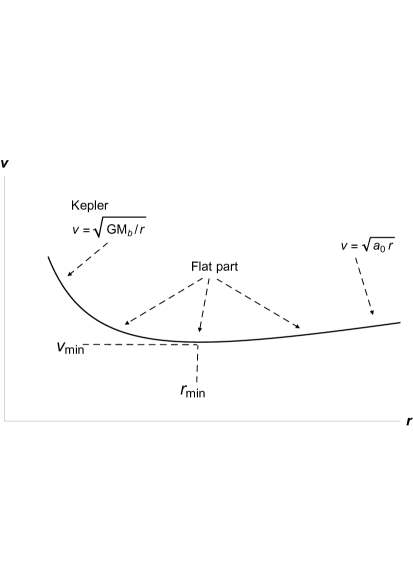
Figure 1: This is a plot of the rotation curve $v=\sqrt{\frac{GM_{b}}{r}+a_{0}r}$. Three parts are clear: the Keplerian part, the flat part around the minimum, and the increasing $\sqrt{a_{0}r}$ part. In galaxies there are no big amounts of baryonic matter outside the flat part and that is why we are not disturbed by the third part. The key is that the constant rotation curve of galaxies is a result of a very flat minimum.

The location of the minimum velocity (the location of the centre of the flat part of the rotation curve) is obtained from the equation $dv/dr=0$, which upon solving gives,

$$r_{min}=\sqrt{\frac{GM_{b}}{a_{0}}}\quad\quad\textrm{(the location of the centre of the flat part)}$$ (2.17)

Note that the larger the mass of the galaxy the more distant the flat part is, and note that a smaller $a_{0}$ makes the flat part further away. The minimum velocity (the constant velocity of the rotation curve) can then be easily computed,

$$v_{min}=\left(4GM_{b}a_{0}\right)^{1/4}\quad\quad\textrm{(the flat velocity)}$$ (2.18)

This last result can be reversed and rewritten as,

$$M_{b}=\frac{v_{min}^{4}}{4Ga_{0}}\quad\quad\textrm{(Baryonic Tully-Fisher relation)}$$ (2.19)

which can be identified with the Baryonic Tully-Fisher relation ($M_{b}\propto v^{4}$, see [15, 16, 17] ), if and only if $a_{0}$ is a universal constant (that does not depend on $M_{b}$). Therefore, we see that the empirical Baryonic Tully-Fisher relation requires that,

$$a_{0}=(\textrm{universal constant})$$ (2.20)

This last statement might not sound strange in our picture because $a_{0}$ (or equivalently $V_{1}$) is supposed to depend on the background fields (in this case on the reservoir of dark matter) and not on the local small system (the baryonic disk of the galaxy); if so then the Baryonic Tully-Fisher relation can be considered as a prediction of our analysis.

As for the width of the flat part of the rotation curve one can calculate the curvature of the curve about the minimum and find,

$$\frac{1}{v_{min}}\left(\frac{d^{2}v}{dr^{2}}\right)_{r_{min}}=\frac{a_{0}}{4GM_{b}}=\frac{1}{4r_{min}^{2}}$$ (2.21)

which is clearly small as it is proportional to $a_{0}$. In more details, if we expand about the minimum, $r=r_{min}+\Delta r$, we get that the velocity is

$$v=v_{min}\left(1+\frac{1}{8}\left(\frac{\Delta r}{r_{min}}\right)^{2}\right)+...$$ (2.22)

where the factor of $1/8$, the squared ratio $\left(\frac{\Delta r}{r_{min}}\right)^{2}$, and the large value of $r_{min}$, all together, tell that the flat part is noticeably wide. Quantitatively, for a typical spiral galaxy the order of magnitude of the flat velocity is $v_{min}\sim 10^{2}\ km/s$ and the order of magnitude of the location of the centre of the flat part is $r_{min}\sim 10\ kpc$. So that, for a displacement $\Delta r\sim 1\ kpc$ one has $(v-v_{min})\sim 10^{-1}\ km/s$ which clearly indicates the existence of a flat minimum in galactic scales (a constant rotation curve).

As for the order of magnitude of the universal constant $a_{0}$ it was found to be

$$a_{0}\sim 10^{-11}\ m/s^{2}$$ (2.23)

This order of magnitude of $a_{0}$ was found by using real data as follows. A typical spiral galaxy has the following approximate ranges for its parameters: the velocity in the flat part $v\in[200,250]\ km/s$, the baryonic mass $M_{b}\in[0.5\times 10^{11},2\times 10^{11}]M_{sun}$, and take a star that lies in the flat part in the range $r\in[30,40]\ kpc$ (see for example the review [21]). With these ranges of parameters, by using $Eq$.(2.16) to extract $a_{0}$, one gets that $a_{0}\sim 10^{-11}\ m/s^{2}$. We have chosen deliberately wide ranges for the parameters to show that the order of magnitude of $a_{0}$ is insensitive which gives further indication that it is a universal constant.

The smallness of $a_{0}$ is an indication of the correctness of the derivative expansion method, in the sense that this makes the linear term $a_{0}r$ (or equivalently $\frac{1}{2}V_{1}r$) change slowly along galactic distances (several kilo-parsecs) and also in the sense that several kilo-parsecs are required before this linear term becomes comparable with the baryonic term $GM_{b}/r$.

As an illustration of all this a plot of the rotation curve of the Milky Way, based on $Eq$.(2.16), is given in $Fig$.2, where we have made a rough estimation that

$$a_{0}=2.8\times 10^{-11}\ m/s^{2}$$ (2.24)

This rough estimation was made by using reasonable approximate values for a single point on the rotation curve of the Milky Way: $r=30\ kpc$, $v=200\ km/s$, and $M_{b}=10^{11}M_{sun}$ (see references [21, 22]). By inserting these values in the rotation curve $Eq.$(2.16) one obtains $a_{0}=2.8\times 10^{-11}\ m/s^{2}$.

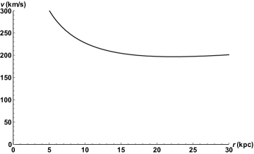
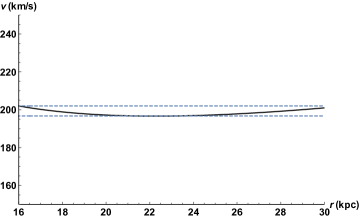
Figure 2: The two plots are taken from reference [20]. Left: This is a plot of the rotation curve of the Milky Way based on $Eq$.(2.16), with parameters $a_{0}=2.8\times 10^{-11}\ m/s^{2}$ and $M_{b}=10^{11}M_{sun}$. The flat part of the rotation curve is clear (concentrated at about $200\ km/s$) and also the Keplerian curve is clear just before the onset of the flat part. Right: Here we zoom in on the flat part (solid line), extending from $16\ kpc$ to $30\ kpc$ along which the velocity lies in the small range $[197\ km/s,202\ km/s]$ bounded by the two dashed lines. Here $r_{min}\approx 22\ kpc$ and $v_{min}\approx 197\ km/s$.

To fix the second constant $U_{1}$ we turn to the Einstein field equations $R_{\mu\nu}-\frac{1}{2}Rg_{\mu\nu}=8\pi GT_{\mu\nu}$. The time-time component gives the following energy density,

$$\rho=\frac{-U_{1}\left(r-GM_{b}\right)}{4\pi Gr^{2}}$$ (2.25)

which in the large radius (Newtonian) limit, $r>>2GM_{b}$, reduces to,

$$\rho=\frac{-U_{1}}{4\pi Gr}$$ (2.26)

On the other hand, in the Newtonian limit the Poisson equation $\nabla^{2}\phi=4\pi G\rho$ governs the physics, where the gravitational potential for our static spacetime is given by $\phi\approx-(g_{00}+1)/2=GM_{b}/r+a_{0}r$. Thus, from the Poisson equation and for $r>0$ one obtains,

$$\rho=\frac{a_{0}}{2\pi Gr}$$ (2.27)

where since we are talking about large $r$’s the delta function is irrelevant.

Thus, by comparing $Eq$.(2.26) with $Eq$.(2.27) we identify,

$$U_{1}=-2a_{0}$$ (2.28)

As a summary, the two first-order constants in the derivative expansion are,

$$V_{1}=-U_{1}=2a_{0}$$ (2.29)

and the metric reads,

$$ds^{2}=-\left(1-\frac{2GM_{b}}{r}+2a_{0}(r-2GM_{b})\right)dt^{2}+\frac{dr^{2}}{1-\frac{2GM_{b}}{r}-2a_{0}(r-2GM_{b})}+r^{2}d\Omega^{2}$$ (2.30)

One can now easily calculate the energy-momentum tensor of dark matter (sourcing this spacetime) by simply plugging the above metric into the Einstein equations, upon which one finds that,

$$T_{\mu}^{\nu}=\textrm{diagonal}(-\rho,P_{r},P_{\perp},P_{\perp})$$ (2.31)

with

$$\rho=\frac{a_{0}}{2\pi Gr}-\frac{a_{0}M_{b}}{2\pi r^{2}}\qquad\quad P_{r}=-\frac{a_{0}M_{b}}{2\pi r^{2}}\qquad\quad P_{\perp}=\frac{a_{0}M_{b}}{4\pi r^{2}}$$ (2.32)

The energy-momentum tensor is that of an anisotropic fluid ($P_{\perp}\neq P_{r}$, see [25]) and was shown in [20] to satisfy the four energy conditions (dominant, weak, null, and strong) outside the black hole horizon, making it clear that this is a physical matter field. Note also that the energy density of dark matter is much larger than the pressures for large radii, a result which is sometimes phrased in the literature by saying that ”dark mater is pressure-less”. Close to the black hole, however, the density and pressures are of the same order of magnitude, signalling a region of relativistic dark matter.

Finally, it is important to mention that our metric $Eq.$ (2.30) and the corresponding rotation curve $Eq.$(2.16) describe a realistic model for galaxies only outside the cores inside which most of the baryonic matter is concentrated; for the milky way that would be about $r>5\ kpc$ (see reference [20]). In our metric we are assuming – as a simplified model – that the baryonic matter of the core is concentrated inside the central black hole at $r=0$. However, if we want to be more precise inside the core we must take the real baryonic matter distribution there into account, that is, we must assume a certain mass density $\rho(r)$ for the baryonic matter inside the core and then solve the Einstein equations. As an illustration, if we assume a constant density of baryonic matter inside the core, $\rho=\textrm{constant}$, then, assuming non-relativistic physics, the velocity will increase linearly with distance like a rigid body, $v\propto r$. Then the combined rotation curve that contains the two regions, inside and outside the core, is given by $Fig.\ref{fig:FIG0}$,

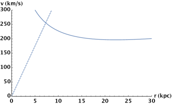
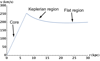
Figure 3: Left: Our plot of the rotation curve (solid line) and the plot of the rotation curve of a rigid body (dashed line), which we took for illustration only, are put together. Right: Since our plot is valid outside the core and the linear curve (straight line) is the model we took inside, the two plots can be merged (in a rough way) together by simply taking off the additional parts after their intersection.

This shows that the Keplerian rise (seen in our rotation curve) does not continue to the centre if real models in the core are assumed. The Keplerian rise in some galaxies (depending on the details) may be very small (barely seen) and in other galaxies may result in a clear peak in the rotation curve – observed rotation curves exhibit these two possibilities.

2.5 Second Order in Derivatives (Cosmology)

In this section we will fix the second order constants $V_{2}$ and $U_{2}$. To do so let us go to the largest scale, that is, to the limit ”$r\rightarrow\infty$”, where the second order terms $\frac{1}{2}V_{2}r^{2}$ and $\frac{1}{2}U_{2}r^{2}$ become dominant over the others in $Eq$.(2.4) and Eq.(2.5). The metric, Eq.(2.2), in this limit reads,

$$ds^{2}=-\left(1+\frac{1}{2}V_{2}r^{2}\right)dt^{2}+\frac{dr^{2}}{1+\frac{1}{2}U_{2}r^{2}}+r^{2}\left(d\theta^{2}+\sin^{2}\theta d\phi^{2}\right)$$ (2.33)

In this limit our metric must coincide with the Friedmann–Lemaître–Robertson–Walker spacetime (this is our boundary condition) since the latter is the spacetime which describes the largest scale; a homogeneous and isotropic universe. As we show in $Sec.$[3] if we take the FLRW metric, expand it in derivatives, and transform coordinates from global to local, then the metric up to second order in derivatives will read,

$$ds^{2}=-\left(1+q_{0}H_{0}^{2}r^{2}\right)dt^{2}+\frac{dr^{2}}{1-\Omega_{0}H_{0}^{2}r^{2}}+r^{2}\left(d\theta^{2}+\sin^{2}\theta d\phi^{2}\right)$$ (2.34)

where $H_{0}$, $q_{0}$, and $\Omega_{0}$ are the well-known cosmological parameters at the present time: $H_{0}$ is the Hubble constant, $q_{0}$ is the deceleration parameter, and $\Omega_{0}$ is the dimensionless density parameter. Thus, the form of our limiting metric $Eq.$(2.33) successfully coincides with the ”expanded” FLRW metric, $Eq.$(2.34), and hence we can identify our constants to be,

$$V_{2}=2q_{0}H_{0}^{2}\qquad\textrm{and}\qquad U_{2}=-2\Omega_{0}H_{0}^{2}$$ (2.35)

2.6 Solar System, Astrophysics, and Cosmology in One Metric, and the Validity of the Derivative Expansion

As an overview we write below the local metric up to second order in derivatives, which accommodates the three distinct scales (solar system, astrophysics, and cosmology) in a single framework:

$$ds^{2}= -\left[1-\frac{2GM_{b}}{r}+2a_{0}(r-2GM_{b})+q_{0}H_{0}^{2}(r-2GM_{b})^{2}\right]dt^{2}$$

$$+\left[1-\frac{2GM_{b}}{r}-2a_{0}(r-2GM_{b})-\Omega_{0}H_{0}^{2}(r-2GM_{b})^{2}\right]^{-1}dr^{2}+r^{2}d\Omega^{2}$$ (2.36)

where the constants $M_{b}$, $a_{0}$, $H_{0}$, $q_{0}$, and $\Omega_{0}$ were defined before.

Stars in Galaxies

For stars in galaxies one can easily calculate the rotation curve up to second order (see Appendix B),

$$v_{\phi}^{2}=rf^{\prime}(r)/2=GM_{b}/r+a_{0}r+q_{0}H_{0}^{2}r^{2}(1-2GM_{b}/r)$$ (2.37)

In the far region of the baryonic black hole, $r>>2GM_{b}$, we can neglect the ratio $2GM_{b}/r$ in the third term and the rotation curve becomes

$$v_{\phi}^{2}=GM_{b}/r+a_{0}r+q_{0}H_{0}^{2}r^{2}$$ (2.38)

The central force in the far region can be easily inferred from the circular motion equation $F_{r}=-mv^{2}/r$, which gives,

$$F_{r}=-GM_{b}m/r^{2}-ma_{0}-mq_{0}H_{0}^{2}r$$ (2.39)

where note that the first two forces are attractive while the third force $-mq_{0}H_{0}^{2}r$ is repulsive because the accelerating expansion of the universe requires $q_{0}<0$.

Galaxies in Clusters

For larger scales (clusters and superclusters) it is commonly assumed that there is no rotation. Galaxies do not rotate in clusters (in contrast to stars in galaxies) but they move radially with respect to the centre of the cluster with a velocity that is a combination of the Hubble flow and some peculiar velocity, $v_{r}=H_{0}r+v_{pec}$. Furthermore, in those large scales the baryonic mass contribution becomes less and less important. Now, the radial acceleration can be obtained from the geodesic equation (see Appendix B.5)

$$\frac{d^{2}r}{dt^{2}}+\left(\frac{h^{\prime}}{2h}-\frac{f^{\prime}}{f}\right)\left(\frac{dr}{dt}\right)^{2}-\frac{f^{2}J^{2}}{r^{3}h}+\frac{f^{\prime}}{2h}=0$$ (2.40)

Since there is no rotation we simply take $J=0$. Since the baryonic contribution is unimportant in those scales we can neglect all terms containing $M_{b}$. Since $dr/dt=v_{r}=H_{0}r+v_{pec}$ with $v_{pec}<<H_{0}r$, the above radial geodesic equation becomes up to second order,

$$\frac{d^{2}r}{dt^{2}} =-\frac{f^{\prime}}{2h}=-a_{0}-\left(q_{0}H_{0}^{2}-2a_{0}^{2}\right)r$$ (2.41)

Finally, one can check that $a_{0}^{2}/H_{0}^{2}\sim 10^{-4}$ and so the $a_{0}^{2}$ term above can be neglected as well, and we are left with the desired result,

$$\frac{d^{2}r}{dt^{2}}=-a_{0}-q_{0}H_{0}^{2}r$$ (2.42)

for the radial acceleration of galaxies in clusters; we see that at leading order galaxies freely fall toward the centre of the cluster with a constant acceleration $a_{0}\sim 10^{-11}\ m/s^{2}$ which tells, in particular, that the cluster is a gravitationally bound system. At next to leading order galaxies are participating in the expansion of the universe with a smaller acceleration $-q_{0}H_{0}^{2}r$.

Clusters and Superclusters

By the same logic one sees that $Eq.$(2.42) applies also to the motion of clusters in superclusters and to the motion of superclusters in the universe, with the difference that now the dark energy term $-q_{0}H_{0}^{2}r$ increases with each higher scale until it becomes comparable and finally larger than the dark matter term $-a_{0}$. The quantitive details follow in the coming section on the validity of the approximation.

Accelerating Expansion

As just said at the largest scale the repulsive force due to dark energy becomes dominant over the dark matter attractive force, and $Eq$.(2.42) becomes,

$$\frac{d^{2}r}{dt^{2}}=-q_{0}H_{0}^{2}r$$ (2.43)

which is the manifestation of the accelerating expansion of the universe in the local metric. In more details, if we use the definition of the deceleration parameter $q_{0}=-\ddot{R}_{0}/R_{0}H_{0}^{2}$ then the last equation can be rewritten as,

$$\frac{d^{2}r}{dt^{2}}/r=\ddot{R}_{0}/R_{0}$$ (2.44)

where remember that the ”dot” indicates a derivative with respect to the cosmological time of the FLRW metric. For the local observer this is the statement that distant galaxies are co-moving with the expanding universe.

Validity of the Approximation Method

It is to be noted that the smallness of the first and second derivatives $V_{1}$, $U_{1}$, $V_{2}$ and $U_{2}$ justifies (and gives strength to) the use of the derivative expansion method. At distances of order $10\ kpc$ (typical size of galaxies), one can check that

$$1>>a_{0}r\sim 10^{-7}>>H_{0}^{2}r^{2}\sim 10^{-11},$$ (2.45)

which is a good start for the derivative expansion method. This tells that it is justified indeed to reach galactic distances by the derivative expansion method. At distances of order $1\ Mpc$ (the typical size of a galaxy cluster) the linear dark matter term is still dominant over the Hubble’s term,

$$a_{0}r\sim 10^{-5}>>H_{0}^{2}r^{2}\sim 10^{-7},$$ (2.46)

which shows that the derivative expansion is still valid and which explains why galaxies in clusters are gravitationally bound systems; from $Eq$.(2.42) we see that dark matter induces an attractive central force $F_{r}=-ma_{0}$ that is much larger than the repulsive force induced by the Hubble’s term, $F_{r}=-mq_{0}H_{0}^{2}r$. At distances of order $10\ Mpc$ (the typical size of a supercluster) the linear term $a_{0}r$ is larger than the Hubble’s term $H_{0}^{2}r^{2}$ by one order of magnitude,

$$a_{0}r\sim 10^{-4}>H_{0}^{2}r^{2}\sim 10^{-5}$$ (2.47)

This again explains why superclusters are gravitationally bound systems as the attractive force due to dark matter is still larger than the repulsive force due to dark energy (see again $Eq$.(2.42)). At distances of order $100\ Mpc$ (the typical size of a large supercluster and larger) the two terms become of the same order,

$$a_{0}r\sim H_{0}^{2}r^{2}\sim 10^{-3}$$ (2.48)

and gravitational systems are not necessarily bound anymore, because the attraction and repulsion are of same order of magnitude. At a distance of order $1000\ Mpc$ (scales much larger than superclusters) the Hubble’s term finally dominates,

$$H_{0}^{2}r^{2}\sim 10^{-1}>a_{0}r\sim 10^{-2}$$ (2.49)

This shows that with the derivative expansion method we can indeed reach large cosmological distances, up to order $1000\ Mpc$. At this stage the expansion of the universe appears in a clear way as there are no bound systems anymore, but everything is flowing with the expansion of universe; because now – see again $Eq$.(2.42) – the repulsive force due to dark energy, $F_{r}=-q_{0}H_{0}^{2}r$, becomes stronger than the attractive force due to dark matter, $F_{r}=-a_{0}$, and so there are no bound systems from this scale and higher.

Yet, we can not go to larger distances by our method because then $H_{0}^{2}r^{2}\sim 1$ and our approximation breaks down, or at best becomes questionable. In any case, there is another reason that prevents us from going to distances much larger than order $1000\ Mpc$ and it is the presence of a cosmological horizon. Since observations favour $\Omega_{0}\approx 1$ one sees that our metric contains a cosmological horizon at $r\approx c/H_{0}\approx 4400\ Mpc$; this horizon is a combination of particle horizon and cosmological event horizon and it is similar to the horizon of static de Sitter spacetime (see for example the references [29, 30] for treating horizons in cosmology). Note that the latter value of the position of the horizon is only approximate, due to our approximation, whereas the real value is larger.

A schematic plot of the function $g_{rr}^{-1}(r)$ is given in $Fig$.4 for the case $\Omega_{0}>0$. A similar schematic plot can be obtained for the redshift function $f(r)=-g_{00}(r)$ as can be checked if you take $q_{0}<0$.

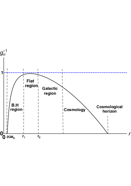
Figure 4: The inverse component $g_{rr}^{-1}$ is plotted (solid line) in a schematic way (not to scale) against the radial coordinate $r$. At the black hole radius $2GM_{b}$ the function vanishes. The region between $r_{1}$ and $r_{2}$ is the location of the locally inertial observer: it is a flat region (with $g_{00}\approx-1$ and $g_{rr}\approx 1$), it is far away from the black hole ($r_{1}>>2GM_{b}$), and it is small enough that the influence of the rest of the universe is negligible. In the regions $r<r_{1}$ and $r>r_{2}$ the function $g_{rr}^{-1}$ does not approximate to unity because the effects of curvature from the black hole and from the rest of the universe become important. The function $g_{rr}^{-1}$ vanishes as well at the position of the cosmological horizon.

We have chosen to plot the function $g_{rr}^{-1}$ because its zeros are the locations of horizons in a static spacetime. In fact, we do not have to worry much about the regularity of the cosmological horizon at this stage because our approximation method is supposed to break down there and higher order terms in the derivative expansion must be taken into account.

2.7 The Energy-Momentum Tensor

The energy-momentum tensor can be obtained easily by inserting the above metric, $Eq$.(2.6), in the Einstein equations,

$$R_{\mu\nu}-\frac{1}{2}Rg_{\mu\nu}=8\pi GT_{\mu\nu}$$ (2.50)

and expanding up to second order in derivatives, upon which one gets that,

$$T_{\mu}^{\nu}=\textrm{diagonal}(-\rho,P_{r},P_{\perp},P_{\perp})$$ (2.51)

where

$$\rho=\frac{a_{0}\left(1-GM_{b}/r\right)}{2\pi Gr}+\frac{3\Omega_{0}H_{0}^{2}}{8\pi G}\left(1-\frac{2GM_{b}}{r}\right)\left(1-\frac{2GM_{b}}{3r}\right)$$ (2.52)

$$P_{r}=-\frac{a_{0}M_{b}}{2\pi r^{2}}-\frac{1}{8\pi G}\left[\Omega_{0}H_{0}^{2}+8a_{0}^{2}-2q_{0}H_{0}^{2}\left(1-\frac{GM_{b}}{r}\right)\right]\left(1-\frac{2GM_{b}}{r}\right)$$ (2.53)

$$P_{\perp}=\frac{a_{0}M_{b}}{4\pi r^{2}}-\frac{1}{8\pi G}\left[\Omega_{0}H_{0}^{2}\left(1-\frac{GM_{b}}{r}\right)^{2}+6a_{0}^{2}-2q_{0}H_{0}^{2}\left(1-\frac{GM_{b}}{r}-\frac{G^{2}M^{2}_{b}}{2r^{2}}\right)\right]$$ (2.54)

where in each of the three expressions, the first term is the first order term and the second term is the second order term. The first order terms were already obtained in [20] and summarised in the previous section, while the second order terms are new results of this work. This energy-momentum tensor encodes information about dark matter (terms coupled to $a_{0}$) and dark energy (terms coupled to $H_{0}$, $q_{0}$, and $\Omega_{0}$) from small distances to very large distances through a nontrivial $r$ dependence.

Note that the energy-momentum tensor is anisotropic ($P_{\perp}\neq P_{r}$). However, at the largest scale (the cosmological scale) it becomes isotropic as expected. To see this let us take the large radius limit ($r\rightarrow\infty$) and obtain,

$$\rho=\frac{3\Omega_{0}H_{0}^{2}}{8\pi G}$$ (2.55)

$$P_{r}=-\frac{1}{8\pi G}\left[\left(\Omega_{0}-2q_{0}\right)H_{0}^{2}+8a_{0}^{2}\right]$$ (2.56)

$$P_{\perp}=-\frac{1}{8\pi G}\left[\left(\Omega_{0}-2q_{0}\right)H_{0}^{2}+6a_{0}^{2}\right]$$ (2.57)

where an anisotropy resulting from the terms $a_{0}^{2}$ still appears. Yet, this is a small anisotropy that can be neglected compared to the $H_{0}^{2}$ terms because

$$\frac{a_{0}^{2}}{H_{0}^{2}c^{2}}\sim 10^{-4}$$ (2.58)

where we have returned $c$ by unit analysis and where we have used the values $H_{0}=2.2\times 10^{-18}\ s^{-1}$ and $a_{0}\sim 10^{-11}\ m/s^{2}$. Therefore, at the cosmological scale we have, indeed, an isotropic energy-momentum tensor with $P_{r}=P_{\perp}\equiv P$, given by

$$\rho=\frac{3\Omega_{0}H_{0}^{2}}{8\pi G}\qquad\qquad P=\frac{-\left(\Omega_{0}-2q_{0}\right)H_{0}^{2}}{8\pi G}$$ (2.59)

One can check that these two last equations are simply the two Friedmann equations of cosmology, written up to second order in derivatives.

3 The Derivative Expansion of the FLRW Metric and the Transformation to the Local Frame

The Friedmann–Lemaître–Robertson–Walker metric is given by,

$$ds^{2}=-d\tau^{2}+R(\tau)^{2}\left[\frac{dr^{\prime 2}}{1-kr^{\prime 2}}+r^{\prime 2}d\Omega^{2}\right]$$ (3.1)

where $\tau$ is the cosmological time, $R(\tau)$ is the scale factor with dimension of length, $r^{\prime}$ is the dimensionless radial co-moving coordinate, $k=\{0,-1,+1\}$ is the curvature parameter, and $d\Omega^{2}=d\theta^{2}+\sin^{2}\theta d\phi^{2}$.

In order to move to the local coordinates, in which the FLRW spacetime takes the Schwarzschild form,

$$ds^{2}=-A(t,r)dt^{2}+B(t,r)dr^{2}+r^{2}d\Omega^{2}$$ (3.2)

we have clearly to perform the coordinate transformation

$$r=R(\tau)r^{\prime}$$ (3.3)

to take care of the angular part, upon which the metric becomes,

$$ds^{2}=-\left[1-\frac{H^{2}r^{2}}{1-kr^{2}/R^{2}}\right]d\tau^{2}-\frac{2Hr}{1-kr^{2}/R^{2}}d\tau dr+\frac{dr^{2}}{1-kr^{2}/R^{2}}+r^{2}d\Omega^{2}$$ (3.4)

where $H(\tau)\equiv\dot{R}(\tau)/R(\tau)$ is the Hubble parameter. Before we go on and cancel the cross term we find it a suitable place to stop and define the derivative expansion of the FLRW metric.

3.1 Defining the Derivative Expansion of the FLRW Metric

To motivate the derivative expansion method for the FLRW metric notice that significant changes of the cosmological metric occurs on large time scales (from the perspective of a local observer) and notice that significant changes in the radial direction also require large distances. In details, let us Taylor expand the scale factor $R(\tau)$ (as it encodes the time dependence of the metric) around the present time $\tau_{0}$,

$$R(\tau)=R(\tau_{0})+\dot{R}(\tau_{0})(\tau-\tau_{0})+\frac{1}{2}\ddot{R}(\tau_{0})(\tau-\tau_{0})^{2}+...$$ (3.5)

or equivalently,

$$R(\tau)=R_{0}\left[1+H_{0}(\tau-\tau_{0})-\frac{1}{2}q_{0}H_{0}^{2}(\tau-\tau_{0})^{2}+...\right]$$ (3.6)

where as usual $R_{0}\equiv R(\tau_{0})$ is the scale factor at the present time, $H_{0}\equiv\dot{R_{0}}/R_{0}$ is the Hubble’s constant, and $q_{0}\equiv-\ddot{R}_{0}R_{0}/\dot{R}_{0}^{2}$ is the deceleration parameter. Pay attention that since $H_{0}$ is very small the hierarchy in the Taylor terms

$$R(\tau_{0})>>\dot{R}(\tau_{0})(\tau-\tau_{0})>>\frac{1}{2}\ddot{R}(\tau_{0})(\tau-\tau_{0})^{2}$$ (3.7)

continues to hold even for large time intervals $\tau-\tau_{0}$ and that is due to the hierarchy in the derivatives

$$O(1)>>O(\partial_{\tau})=O(H_{0})>>O(\partial^{2}_{\tau})=O(H_{0}^{2})$$ (3.8)

As for the radial direction notice that the coordinate $r$ appears in the metric, $Eq$.(3.4), only through the ratio $r/R$, where we are excluding the angular part $r^{2}d\Omega^{2}$ from our discussion as it is already in the Schwarzschild form and so we will leave it as it is. Since the scale factor $R$ is very large it is clear that significant changes along the radial direction $r$ require large distances for a local observer. More precisely, if we Taylor expand any component of the metric $g(r)$ around $r=0$ we get,

$$g(r)=g(0)+\partial_{r}g(0)r+\frac{1}{2}\partial^{2}_{r}g(0)r^{2}+...=g(0)+\frac{\partial_{x}g(0)}{R}r+\frac{1}{2}\frac{\partial^{2}_{x}g(0)}{R^{2}}r^{2}+...$$ (3.9)

where $x=r/R$. Thus, similar to the case of time derivatives discussed above, here as well the generic hierarchy in the Taylor terms

$$g(0)>>\partial_{r}g(0)r>>\frac{1}{2}\partial^{2}_{r}g(0)r^{2}$$ (3.10)

continues to hold even for large $r$’s and that is because of the hierarchy in the derivatives

$$O(1)>>O(\partial_{r})=O(1/R)>>O(\partial^{2}_{r})=O(1/R^{2})$$ (3.11)

One more comment deserves being made. By looking at one of the Friedman equations,

$$\frac{\dot{R}^{2}}{R^{2}}=\frac{8\pi G}{3}\rho-\frac{k}{R^{2}}$$ (3.12)

one can see that generically the term $k/R^{2}$ is of the same order as $\dot{R}^{2}/R^{2}$ because they are terms in the same equation. Therefore, since $k/R^{2}=O(\partial^{2}_{r})$ and $\dot{R}^{2}/R^{2}=H^{2}=O(\partial^{2}_{\tau})$ we conclude that the time derivative and the radial derivative are generically of the same order,

$$O(\partial_{r})=O(\partial_{\tau})$$ (3.13)

3.2 The FLRW Spacetime in the Local Frame

Now we can go on and expand the FLRW metric Eq.(3.4) up to second order in derivatives and obtain,

$$ds^{2}=-\left[1-H_{0}^{2}r^{2}\right]d\tau^{2}-2\left[H_{0}+\dot{H}_{0}(\tau-\tau_{0})\right]rd\tau dr+\left[1+kr^{2}/R_{0}^{2}\right]dr^{2}+r^{2}d\Omega^{2}$$ (3.14)

To cancel the cross term we perform a general coordinate transformation of the form

$$\tau=\tau(t,r)$$ (3.15)

after which we get (all subsequent calculations are going to be up to second order in derivatives),

$$ds^{2} =-\left[1-H_{0}^{2}r^{2}\right]\left(\frac{\partial\tau}{\partial t}\right)^{2}dt^{2}-2\frac{\partial\tau}{\partial t}\left(\left[H_{0}+\dot{H}_{0}(\tau-\tau_{0})\right]r+\left[1-H_{0}^{2}r^{2}\right]\frac{\partial\tau}{\partial r}\right)dtdr$$

$$+\left(1+kr^{2}/R_{0}^{2}-\left[1-H_{0}^{2}r^{2}\right]\left(\frac{\partial\tau}{\partial r}\right)^{2}-2\left[H_{0}+\dot{H}_{0}(\tau-\tau_{0})\right]r\frac{\partial\tau}{\partial r}\right)dr^{2}+r^{2}d\Omega^{2}$$ (3.16)

To achieve $g_{tr}=0$ we must require that,

$$\frac{\partial\tau}{\partial r}=-\left[H_{0}+\dot{H}_{0}(\tau-\tau_{0})\right]r$$ (3.17)

Upon integration with respect to $r$ this yields,

$$\tau=-\frac{1}{2}\left[H_{0}+\dot{H}_{0}(\tau-\tau_{0})\right]r^{2}+\psi(t)$$ (3.18)

where $\psi(t)$ is an arbitrary (gauge) function of $t$. By inserting equation Eq.(3.18) into Eq.(3.2) one obtains,

$$ds^{2}=-\left[\left(\frac{d\psi}{dt}\right)^{2}-\left(H_{0}^{2}\left(\frac{d\psi}{dt}\right)^{2}+\dot{H}_{0}\frac{d\psi}{dt}\right)r^{2}\right]dt^{2}+\left[1+\left(H_{0}^{2}+\frac{k}{R_{0}^{2}}\right)r^{2}\right]dr^{2}+r^{2}d\Omega^{2}$$ (3.19)

We will choose the gauge,

$$d\psi/dt=1$$ (3.20)

in order to make $g_{tt}=-1$ at very small $r$’s since we are talking about the coordinates of a locally inertial observer. One can also easily check that,

$$\dot{H}_{0}=-\left(1+q_{0}\right)H_{0}^{2}$$ (3.21)

All in all, the metric Eq.(3.19) reads now,

$$ds^{2}=-\left(1+q_{0}H_{0}^{2}r^{2}\right)dt^{2}+\frac{dr^{2}}{1-\left(H_{0}^{2}+\frac{k}{R_{0}^{2}}\right)r^{2}}+r^{2}d\Omega^{2}$$ (3.22)

which has the required form. The last step is going to be for the sake of appearance only, and it is to use the definition of the dimensionless density parameter $\Omega_{0}=\left(H_{0}^{2}+\frac{k}{R_{0}^{2}}\right)/H_{0}^{2}$ and to rewrite the above metric in the final desired form,

$$ds^{2}=-\left(1+q_{0}H_{0}^{2}r^{2}\right)dt^{2}+\frac{dr^{2}}{1-\Omega_{0}H_{0}^{2}r^{2}}+r^{2}d\Omega^{2}$$ (3.23)

This is the FLRW spacetime written in the local coordinates $(t,r)$ up to second order in derivatives. It is to be said that this metric was found before in [4] by using a different approximation scheme. It is important to notice that the metric is static; the time-dependence does not appear at this order. The above FLRW metric (with a precision of order $H_{0}^{2}$) is supposed to cover many observations in cosmology. As will be shown in the next section this metric covers the region of small redshifts with $z<1$. For large redshifts, that is, for $z>1$, we must restore to the full FLRW metric.

4 The Cosmological Redshift from the Local Metric

In this section we firstly show how the cosmological redshift $z$ is obtained from the local metric and that it coincides with the familiar formula in the literature up to order $H_{0}^{2}$. Secondly, we show that up to this order the cosmological redshift is the sum of two effects: a gravitational shift and a special-relativistic Doppler redshift.

4.1 Calculation of the Cosmological Redshift

At cosmological distances the baryonic contributions become negligible and the local metric $Eq$.(2.6) reads,

$$ds^{2}=-fdt^{2}+hdr^{2}+r^{2}d\Omega^{2}=-\left(1+2a_{0}r+q_{0}H_{0}^{2}r^{2}\right)dt^{2}+\frac{dr^{2}}{1-2a_{0}r-\Omega_{0}H_{0}^{2}r^{2}}+r^{2}d\Omega^{2}$$ (4.1)

where we have neglected all terms containing the baryonic mass $M_{b}$ and kept the terms of dark matter and dark energy.

Take a galaxy with 4-velocity $V^{\mu}$ which sends a light signal toward us (relative to such large distances we are almost at the centre of the local coordinates $r=0$) with a wave vector $K^{\mu}=(K^{0},K^{r},0,0)$. The frequency of the emitted light as measured by the galaxy (the source) is $\omega_{s}=-K_{\mu}V^{\mu}$ evaluated at the position and time of emission $(t,r,\theta,\phi)$. Similarly, the frequency observed on Earth is $\omega_{o}=-K_{\mu}U^{\mu}$ evaluated at the position and time of observation $(t=0,r=0)$, where $U^{\mu}=(1,\vec{0})$ is the 4-velocity of the stationary observer situated at $r=0$. After using the conditions $V_{\mu}V^{\mu}=-1$ and $K_{\mu}K^{\mu}=0$ one obtains for the ingoing null ray and for the galaxy respectively,

$$K^{r}=-\sqrt{\frac{f}{h}}K^{0}\qquad\textrm{and}\qquad V^{0}=\frac{1}{\sqrt{f-h(\frac{dr}{dt})^{2}-r^{2}(\frac{d\phi}{dt})^{2}}}$$ (4.2)

where we have used the relations $V^{0}=\frac{dt}{d\tau}$, $V^{r}=\frac{dr}{d\tau}=\frac{dt}{d\tau}\frac{dr}{dt}=V^{0}\frac{dr}{dt}$, $V^{\phi}=\frac{d\phi}{d\tau}=V^{0}\frac{d\phi}{dt}$, and $V^{\theta}=0$ ^,. Since our metric is static with a corresponding killing vector $\xi^{\mu}=(dt)^{\mu}$ the energy of particles is conserved and we have $K_{\mu}\xi^{\mu}=\textrm{constant}$; this gives that $K^{0}(r)=K^{0}(0)/f(r)$.

Thus the frequency of the light ray as measured by the galaxy is,

$$\omega_{s}=-K_{\mu}V^{\mu}|_{(t,r)}=\frac{K^{0}(0)}{f(r)}\frac{f(r)+\sqrt{f(r)h(r)}\frac{dr}{dt}}{\sqrt{f(r)-h(r)(\frac{dr}{dt})^{2}-r^{2}(\frac{d\phi}{dt})^{2}}}$$ (4.3)

and the observed frequency on Earth is,

$$\omega_{o}=-K_{\mu}U^{\mu}|_{(t=0,r=0)}=K^{0}(0)$$ (4.4)

The redshift is therefore,

$$z=\frac{\omega_{s}}{\omega_{o}}-1=\frac{1}{\sqrt{f}}\frac{1+\sqrt{\frac{h}{f}}\frac{dr}{dt}}{\sqrt{1-\frac{h}{f}(\frac{dr}{dt})^{2}-\frac{r^{2}}{f}(\frac{d\phi}{dt})^{2}}}-1$$ (4.5)

By writing $dr/dt=v_{r}$ and $rd\phi/dt=v_{\phi}$ the redshift formula becomes,

$$z=\frac{1}{\sqrt{f}}\frac{1+\sqrt{\frac{h}{f}}v_{r}}{\sqrt{1-\frac{h}{f}v_{r}^{2}-\frac{1}{f}v_{\phi}^{2}}}-1$$ (4.6)

If the spacetime were flat, $f=h=1$, we would recover the special relativistic Doppler effect,

$$z=\frac{1+v_{r}}{\sqrt{1-(\vec{v})^{2}}}-1$$ (4.7)

If the emitting source were static we would obtain the purely gravitational shift,

$$z=\frac{1}{\sqrt{f}}-1$$ (4.8)

Going back to the full formula, $Eq.$(4.6), recall that in this particle-dynamics treatment of galaxies the initial distances and initial velocities of galaxies must be supplied by us as part of the initial value problem. Notice that the $r$, $v_{r}$, and $v_{\phi}$, appearing in the redshift formula $Eq.$(4.6) are the coordinate distance of the galaxy and its velocity components at the time of emission and hence can be taken as initial values. Galaxies in clusters are commonly known ”not” to have rotation about the centre of the cluster, that is, $v_{\phi}\approx 0$, while the radial velocity is observed to correspond to the Hubble flow plus some peculiar velocity,

$$v_{r}=H_{0}r+v_{pec}$$ (4.9)

It is to be said before we proceed that in this section the use of the coordinate distance $r$ or the proper distance $D$ to the galaxy (at the time of emission) does not change the results, because as can be checked,

$$D=\int_{0}^{r}\sqrt{h(r)}dr=r+O(a_{0})$$ (4.10)

which would give a correction of order $O(a_{0}H_{0})$ to the Hubble’s law which is smaller than the order $O(H_{0}^{2})$, up to which we want to work; one can check that $a_{0}/H_{0}\sim 10^{-2}$.

Now if we expand the full expression of the redshift $Eq$.(4.6) up to second order in derivatives by using our initial conditions $v_{\phi}\approx 0$ and $v_{r}=H_{0}r+v_{pec}$ (we are interested in cases where the peculiar velocity is very small compared to the Hubble flow, $v_{pec}=O(H_{0}^{2}r^{2})$ or smaller), then we obtain after some work,

$$z=H_{0}\left(1-\frac{a_{0}}{H_{0}}\right)r+\frac{1}{2}\left(1-q_{0}-2\frac{a_{0}}{H_{0}}+3\frac{a_{0}^{2}}{H_{0}^{2}}\right)H_{0}^{2}r^{2}+v_{pec}$$ (4.11)

In the second parenthesis $a_{0}^{2}/H_{0}^{2}\sim 10^{-4}$ and $a_{0}/H_{0}\sim 10^{-2}$ and so can be neglected since they give rise to terms much smaller than order $H_{0}^{2}$, and so,

$$z=H_{0}\left(1-\frac{a_{0}}{H_{0}}\right)r+\frac{1}{2}\left(1-q_{0}\right)H_{0}^{2}r^{2}+v_{pec}$$ (4.12)

The ratio $a_{0}/H_{0}\sim 10^{-2}$ is within the error in determining the value of Hubble’s constant, but nevertheless, it can not be ignored, in principle, if we are going to next order terms. Instead, we can rescale the Hubble’s constant by defining the observed Hubble’s constant,

$$H_{0}^{obs}\equiv H_{0}\left(1-\frac{a_{0}}{H_{0}}\right)$$ (4.13)

after which one obtains,

$$z=H^{obs}_{0}r+\frac{1}{2}\left(1-q_{0}\right)(H_{0}^{obs})^{2}r^{2}+v_{pec}$$ (4.14)

Since, as stated above, the initial peculiar velocity $v_{pec}$ is of the order of $H_{0}^{2}r^{2}$ or smaller we can write it as

$$v_{pec}=\frac{C}{2}(H_{0}^{obs})^{2}r^{2}$$ (4.15)

where $C$ is a constant that must be determined by the initial conditions. Upon this we obtain,

$$z=H^{obs}_{0}r+\frac{1}{2}\left(1-q_{0}+C\right)(H_{0}^{obs})^{2}r^{2}$$ (4.16)

If this last equation is inverted one obtains $r$ in terms of $z$,

$$r=\frac{1}{H_{0}^{obs}}\left[z-\frac{1}{2}\left(1-q_{0}+C\right)z^{2}\right]$$ (4.17)

To coincide with the literature (see for example [18, 26, 27]) we must fix

$$C=2q_{0}$$ (4.18)

upon which one gets the familiar distance-redshift relation for small redshifts ($z<1$),

$$r=\frac{1}{H_{0}^{obs}}\left[z-\frac{1}{2}\left(1+q_{0}\right)z^{2}\right]$$ (4.19)

which is the goal of this section.

It is worth to conclude this section with the following comment. After fixing the constant $C$ the velocity of the source galaxy at the time of emission, $Eq$.(4.9), can be written as

$$v_{r}=H_{0}r+q_{0}H_{0}^{2}r^{2}$$ (4.20)

where it does not differ whether we used $H_{0}$ or $H_{0}^{obs}$ as long as we are working up to order $H_{0}^{2}$. Since the light was sent from the source galaxy at negative time $t$ and received on Earth at time $t=0$ one can write $r=-t$ for the distance to the galaxy. Then one can write $v_{r}=v_{0}+at$, describing motion at constant acceleration in flat spacetime, where $v_{0}=H_{0}r$ is the initial velocity and $a=-q_{0}H_{0}^{2}r$ is the cosmological acceleration – see $Eq$.(2.43). This comment shows that the value we have fixed for the constant $C$ is consistent with the physical cosmological picture as it tells that the galaxy is accelerating at the rate of the cosmological acceleration of the universe.

4.2 The Cosmological Redshift is the Sum of Doppler and Gravitational Shifts

The special-relativistic Doppler shift from a source receding from a static observer at a constant velocity along the line of sight is given by,

$$z_{dop}=\frac{\omega_{s}}{\omega_{o}}-1=\sqrt{\frac{1+\beta}{1-\beta}}-1=\beta+\frac{1}{2}\beta^{2}+...$$ (4.21)

where $\beta$ is the velocity of the source and where we have expanded up to order $\beta^{2}$. In our case $\beta$ is the recessional velocity of some galaxy (that is, $\beta=H_{0}r+v_{pec}$) and so,

$$z_{dop}=H_{0}r+\frac{1}{2}H_{0}^{2}r^{2}+v_{pec}+...$$ (4.22)

where we have assumed as usual $v_{pec}<<H_{0}r$. The gravitational shift, on the other hand, in a light ray sent from a static source at distance $r$ and received by an observer at $r=0$ in our static spacetime is given by,

$$z_{grav}=\frac{1}{\sqrt{f(r)}}-1=-a_{0}r+\frac{1}{2}\left(-q_{0}+3\frac{a_{0}^{2}}{H_{0}^{2}}\right)H_{0}^{2}r^{2}+...$$ (4.23)

The total frequency shift is the sum of the above two shifts,

$$z=z_{dop}+z_{grav}=H_{0}\left(1-\frac{a_{0}}{H_{0}}\right)r+\frac{1}{2}\left(1-q_{0}+3\frac{a_{0}^{2}}{H_{0}^{2}}\right)H_{0}^{2}r^{2}+v_{pec}$$ (4.24)

By repeating the same approximations, the same rescaling of the Hubble’s constant, and the same treatment for $v_{pec}$, done in the previous section, we reproduce exactly the same cosmological redshift $z$ given in Eq.(4.16) which is the goal of this section. The redshift analysis of the previous section is more general and more complete than the one performed here. However, the different effects contributing to the redshift are entangled in one formula, Eq.(4.6), and are not split neatly from each other. The goal of this section was to split the contributing effects from each other and to identify each of them separately. A similar analysis was done for example in [28] but was restricted to specific cosmologies; the authors stated that the breaking of the full effect into two components (doppler and static gravitational shift) can be obtained in static universes only. Here we have shown that this breaking occurs for all cosmologies as long as we are working up to order $H_{0}^{2}$.

5 Discussion

The main result of this paper is to put the three significant scales - the solar system, the galactic, and the cosmological scales - in one framework. The unifying framework is argued to be the derivative expansion method. This framework can be seen as the natural one if we think from the point of view of a locally inertial observer, like us, as was discussed in detail in the bulk of the paper. In what follows we are going to give several comments that are thought to be important:

1. The galactic scale was missed in the previous works trying to connect the solar system with cosmology – see for instance [1, 2, 3, 4, 5, 6]. In this work it is shown that the galactic scale (first order in derivatives) connects the latter two scales. It is to be said that linear terms (in $r$) in the metric components $g_{00}$ and $g_{rr}$ were never correlated before [20] with dark matter, in contrast to quadratic terms (proportional to $r^{2}$) which were long ago correlated with dark energy. The consistency of the approach together with its success at giving the main observations in each scale give further support that those linear terms are indeed related to dark matter.

2. This framework suggests a new possible view of dark matter and dark energy. Dark matter and dark energy could be different ”projections” of the same matter field. That is, there could be a single dark field in space that changes very slowly, and so when it is Taylor expanded – that is, when we expand $V(r)$ and $U(r)$ – the first order terms are what we call dark matter and the second order terms are what we call dark energy.

3. When we talk about some distance $r$ then by the parameter $M_{b}$ we mean the baryonic mass inside this radius. If $r$ is just outside the solar system then $M_{b}$ is almost the mass of the Sun, if $r$ is just outside a galaxy then $M_{b}$ is the baryonic mass of the galaxy, and if $r$ is just outside a cluster of galaxies then $M_{b}$ is the baryonic mass of the cluster. It is interesting to note how our method was applied also to galaxy clusters. In $Sec.[$2.6] it was shown that our analysis predicts that galaxies in clusters are freely falling toward the centre of the cluster with a constant acceleration $a_{0}\sim 10^{-11}\ m/s^{2}$, and at the same time moving collectively along with the Hubble’s flow.

4. The spacetime proposed in this work (up to second order in derivatives) is anisotropic and the anisotropy is expressed by the result that the radial and perpendicular pressures of dark matter and dark energy are unequal, $P_{r}\neq P_{\perp}$, in general. It is interesting to see how our metric restores the isotropy when we take the limit of very large $r$. The same comment holds also for the energy-momentum tensor.

5. Finally, we would like to stress that our constructed metric is a local one (corresponding to small redshifts, $z<1$). Yet our local metric is valid up to great distances, up to distances that are only one order of magnitude smaller than the distance to the cosmological horizon (see $Sec.$ 2.6 and the discussion about validity). In numbers, our local metric is valid up to distances of order $1000\ Mpc$ (corresponding to $z<1$) while the distance to the cosmological horizon is of order $10,000\ Mpc$. Distances corresponding to large $z$ are packed close to the cosmological horizon.

   In order to discuss large redshifts ($z>1$) the time-dependence of the FLRW metric must be taken into account since such redshifts correspond to light rays sent at times when the scale factor of the universe was considerably smaller than at present. Thus our static local metric is not valid in this regime. In this case one simply has to turn to the FLRW metric which is our boundary condition. However, if one wishes one can continue with the derivative expansion method up to third order and higher but allow now for the time-dependence to enter; that is, one has to perform the derivative expansion in both the $r$ and $t$ coordinates and one has to match the local metric with the global FLRW metric in the matching region. From the local metric point of view the matching region is the large radius limit. The matching is done by fixing the higher order coefficients of the local metric so as to coincide with the FLRW metric (expanded up to the relevant order).

Appendix A Eddington-Finkelstein Coordinates and Regularity of the Horizon

Since we have spherical symmetry, in order to find the location of the horizon we look for the null $r=\textrm{constant}$ surface,

$$g^{\mu\nu}\partial_{\mu}r\partial_{\nu}r=0$$ (A.1)

which for our metric $Eq$.(2.2) gives

$$g^{rr}=h^{-1}=0$$ (A.2)

To make the horizon regularity manifest we move to the new coordinate $v=t+r_{*}$ where $dr_{*}/dr=\sqrt{h/f}$, upon which our metric $Eq$.(2.2) becomes

$$ds^{2}=-f(r)dv^{2}+2\sqrt{f(r)h(r)}dvdr+r^{2}\left(d\theta^{2}+\sin^{2}\theta d\phi^{2}\right)$$ (A.3)

In order to prevent a singularity in $g_{rv}$ at the horizon (as $h\rightarrow\infty$) clearly we must have

$$f(r)=h(r)^{-1}\qquad\textrm{as}\qquad r\rightarrow r_{0}$$ (A.4)

Appendix B Geodesic Equation in Spherically Symmetric Static Spacetimes

For the general spherically symmetric static metric

$$ds^{2}=-f(r)dt^{2}+h(r)dr^{2}+r^{2}\left(d\theta^{2}+\sin^{2}\theta d\phi^{2}\right)$$ (B.1)

the geodesic equations are

$$\frac{d^{2}x^{\mu}}{dp^{2}}+\Gamma^{\mu}_{\nu\lambda}\frac{dx^{\nu}}{dp}\frac{dx^{\lambda}}{dp}=0$$ (B.2)

where $p$ is a parameter along the trajectory. Because of spherical symmetry the motion will take place in a plane, and without loss of generality we will take it to be in the $\theta=\pi/2$ plane. The radial equation of motion will be (here we are going to follow reference [18])

$$\frac{d^{2}r}{dp^{2}}+\frac{h^{\prime}}{2h}\left(\frac{dr}{dp}\right)^{2}-\frac{J^{2}}{r^{3}h}+\frac{f^{\prime}}{2hf^{2}}=0$$ (B.3)

where the prime denotes derivative with respect to $r$. There are also the two familiar relations

$$\frac{dt}{dp}=\frac{1}{f(r)}\qquad\textrm{and}\qquad r^{2}\frac{d\phi}{dp}=J$$ (B.4)

where the constant $J$ is the angular momentum per unit mass. In terms of the time coordinate $t$ the radial equation becomes,

$$\frac{d^{2}r}{dt^{2}}+\left(\frac{h^{\prime}}{2h}-\frac{f^{\prime}}{f}\right)\left(\frac{dr}{dt}\right)^{2}-\frac{f^{2}J^{2}}{r^{3}h}+\frac{f^{\prime}}{2h}=0$$ (B.5)

For a circular motion, $r=\textrm{constant}$, the equation B.5 simply becomes

$$\frac{J^{2}}{r^{3}}=\frac{f^{\prime}}{2f^{2}}$$ (B.6)

On the other hand, upon combining the two equations in B.4 one gets that

$$J=r^{2}\frac{d\phi}{dt}f^{-1}$$ (B.7)

Finally, if we insert equation B.7 into equation B.6 we get

$$\frac{(v_{\phi})^{2}}{r}=\frac{1}{2}f^{\prime}$$ (B.8)

where $v_{\phi}=rd\phi/dt$ is the angular velocity. Thus, finally, the rotation curve for circular orbits takes the simple form,

$$(v_{\phi})^{2}=\frac{1}{2}f^{\prime}r$$ (B.9)

References

- [1] G. C. McVittie, “The mass-particle in an expanding universe,” Mon. Not. Roy. Astron. Soc. 93 (1933), 325-339 doi:10.1093/mnras/93.5.325
- [2] A. Einstein and E. G. Straus, “The influence of the expansion of space on the gravitation fields surrounding the individual stars,” Rev. Mod. Phys. 17 (1945), 120-124 doi:10.1103/RevModPhys.17.120
- [3] F. I. Cooperstock, V. Faraoni and D. N. Vollick, “The Influence of the cosmological expansion on local systems,” Astrophys. J. 503 (1998), 61 doi:10.1086/305956 [arXiv:astro-ph/9803097 [astro-ph]].
- [4] M. Mizony and M. Lachieze-Rey, “Cosmological effects in the local static frame,” Astron. Astrophys. 434 (2005), 45-52 doi:10.1051/0004-6361:20042195 [arXiv:gr-qc/0412084 [gr-qc]].
- [5] V. Faraoni and A. Jacques, “Cosmological expansion and local physics,” Phys. Rev. D 76 (2007), 063510 doi:10.1103/PhysRevD.76.063510 [arXiv:0707.1350 [gr-qc]].
- [6] A. Mitra, “Friedmann-Robertson-Walker metric in curvature coordinates and its applications,” Grav. Cosmol. 19 (2013), 134-137 doi:10.1134/S0202289313020072
- [7] F. K. Manasse and C. W. Misner, “Fermi Normal Coordinates and Some Basic Concepts in Differential Geometry,” J. Math. Phys. 4 (1963), 735-745 doi:10.1063/1.1724316
- [8] W. T. Ni and M. Zimmermann, “Inertial and gravitational effects in the proper reference frame of an accelerated, rotating observer,” Phys. Rev. D 17 (1978), 1473-1476 doi:10.1103/PhysRevD.17.1473
- [9] K. P. Marzlin, “On the physical meaning of Fermi coordinates,” Gen. Rel. Grav. 26 (1994), 619 doi:10.1007/BF02108003 [arXiv:gr-qc/9402010 [gr-qc]].
- [10] C. W. Misner, K. S. Thorne and J. A. Wheeler, “Gravitation,”
- [11] E. Pajer, F. Schmidt and M. Zaldarriaga, “The Observed Squeezed Limit of Cosmological Three-Point Functions,” Phys. Rev. D 88 (2013) no.8, 083502 doi:10.1103/PhysRevD.88.083502 [arXiv:1305.0824 [astro-ph.CO]].
- [12] L. Dai, E. Pajer and F. Schmidt, “On Separate Universes,” JCAP 10 (2015), 059 doi:10.1088/1475-7516/2015/10/059 [arXiv:1504.00351 [astro-ph.CO]].
- [13] G. Cabass, E. Pajer and F. Schmidt, “How Gaussian can our Universe be?,” JCAP 01 (2017), 003 doi:10.1088/1475-7516/2017/01/003 [arXiv:1612.00033 [hep-th]].
- [14] L. Dai, E. Pajer and F. Schmidt, “Conformal Fermi Coordinates,” JCAP 11 (2015), 043 doi:10.1088/1475-7516/2015/11/043 [arXiv:1502.02011 [gr-qc]].
- [15] R. B. Tully and J. R. Fisher, “A New method of determining distances to galaxies,” Astron. Astrophys. 54 (1977) 661.
- [16] S. S. McGaugh, J. M. Schombert, G. D. Bothun and W. J. G. de Blok, “The Baryonic Tully-Fisher relation,” Astrophys. J. 533 (2000) L99 doi:10.1086/312628 [astro-ph/0003001].
- [17] S. McGaugh, “The Baryonic Tully-Fisher Relation of Gas Rich Galaxies as a Test of LCDM and MOND,” Astron. J. 143 (2012) 40 doi:10.1088/0004-6256/143/2/40 [arXiv:1107.2934 [astro-ph.CO]].
- [18] S. Weinberg, “Gravitation and Cosmology : Principles and Applications of the General Theory of Relativity”, (New York : Wiley, 1972), isbn: 978-0-471-92567-5
- [19] R. M. Wald, “General Relativity,” doi:10.7208/chicago/9780226870373.001.0001
- [20] F. Haddad and N. Haddad, “A Black Hole inside Dark Matter and the Rotation Curves of Galaxies,” International Journal of Modern Physics D Vol. 29, No. 15, 2050107 (2020), doi:10.1142/S0218271820501072 [arXiv:2002.12772 [gr-qc]].
- [21] Y. Sufue, ”Rotation and mass in the Milky Way and spiral galaxies”, Publications of the Astronomical Society of Japan, Volume 69, Issue 1, February 2017, R1, https://doi.org/10.1093/pasj/psw103
- [22] Y. Sufue, ”Dark halos of M31 and the Milky Way”, Publications of the Astronomical Society of Japan, Volume 67, Issue 4, August 2015, 75, https://doi.org/10.1093/pasj/psv042
- [23] M. Milgrom, “MOND theory,” Can. J. Phys. 93 (2015) no.2, 107-118 doi:10.1139/cjp-2014-0211 [arXiv:1404.7661 [astro-ph.CO]].
- [24] M. Milgrom, “MOND vs. dark matter in light of historical parallels,” Stud. Hist. Phil. Sci. B 71 (2020), 170-195 doi:10.1016/j.shpsb.2020.02.004 [arXiv:1910.04368 [astro-ph.GA]].
- [25] R. L. Bowers and E. P. T. Liang, “Anisotropic Spheres in General Relativity,” Astrophys. J. 188 (1974) 657. doi:10.1086/152760
- [26] S. Weinberg, “Cosmology,” Published in: Oxford, UK: Oxford Univ. Pr. (2008) 593 p ISBN: 9780198526827
- [27] B. Ryden, “Introduction to cosmology,” Published in: San Francisco, USA: Addison-Wesley (2003) 244 p ISBN: 9781107154834 (Print), 9781316889848
- [28] A. B. Whiting, “The Expansion of space: Free particle motion and the cosmological redshift,” Observatory 124 (2004), 174 [arXiv:astro-ph/0404095 [astro-ph]].
- [29] S. Hawking, G. Ellis, (1973). ”The Large Scale Structure of Space-Time” (Cambridge Monographs on Mathematical Physics). Cambridge: Cambridge University Press. doi:10.1017/CBO9780511524646
- [30] E. Harrison, ”Hubble Spheres and Particle Horizons”, (1991) Astrophysical Journal v.383, p.60, doi:10.1086/170763