Making transport more robust and interpretable by moving data
through a small number of anchor points

Abstract

Optimal transport (OT) is a widely used technique for distribution alignment, with applications throughout the machine learning, graphics, and vision communities. Without any additional structural assumptions on transport, however, OT can be fragile to outliers or noise, especially in high dimensions. Here, we introduce Latent Optimal Transport (LOT ), a new approach for OT that simultaneously learns low-dimensional structure in data while leveraging this structure to solve the alignment task. The idea behind our approach is to learn two sets of “anchors” that constrain the flow of transport between a source and target distribution. In both theoretical and empirical studies, we show that LOT regularizes the rank of transport and makes it more robust to outliers and the sampling density. We show that by allowing the source and target to have different anchors, and using LOT to align the latent spaces between anchors, the resulting transport plan has better structural interpretability and highlights connections between both the individual data points and the local geometry of the datasets.

1 Introduction

Optimal transport (OT) (Villani, 2008) is a widely used technique for distribution alignment that learns a transport plan which moves mass from one distribution to match another. With recent advances in tools for regularizing and speeding up OT (Cuturi, 2013), this approach has found applications in many diverse areas of machine learning, including domain adaptation (Courty et al., 2014, 2017), generative modeling (Martin Arjovsky & Bottou, 2017; Tolstikhin et al., 2017), document retrieval (Kusner et al., 2015), computer graphics (Solomon et al., 2014, 2015; Bonneel et al., 2016), and computational neuroscience (Gramfort et al., 2015; Lee et al., 2019).

While the ground metric in OT can be used to impose geometric structure into transport, without any additional assumptions, OT can be fragile to outliers or noise, especially in high dimensions. To overcome this issue, additional structure, either in the data or in the transport plan, can be used to improve alignment or make transport more robust. Examples of methods that incorporate additional structure into OT include approaches that leverage hierarchical structure or cluster consistency (Lee et al., 2019; Yurochkin et al., 2019; Xu et al., 2020), partial class information (Courty et al., 2017, 2014), submodular cost functions (Alvarez-Melis et al., 2018), and low-rank constraints on the transport plan (Forrow et al., 2019; Altschuler et al., 2019). Because of the difficulty of incorporating structure into OT, many of these methods need low-dimensional structure in data to be specified in advance (e.g., estimated clusters or labels).

To simultaneously learn low-dimensional structure and use it to constrain transport, Forrow et al. (2019) recently introduced a statistical approach for OT that builds a factorization of the transport plan to regularize its rank. After factorization, transport from a source to target distribution can be visualized as the flow of mass through a small number of anchors (hubs), which serve as relay stations through which transportation must pass (see Figure 1, a vs. b). Although this idea of moving data through anchors is appealing, in previous work, the anchors used to constrain transport are shared by the source and target. As a result, when the source and target contain different structures or experience domain shift (Courty et al., 2014), shared anchors may not provide an adequate representation for both domains simultaneously.

In this work, we propose a new structured transport approach called Latent Optimal Transport (LOT ). The main idea behind LOT is to factorize the transport plan into three components, where mass is moved: (i) from individual source points to source anchors, (ii) from the source anchors to target anchors, and (iii) from target anchors to individual target points (Figure 1c-d). The intermediate transport plan captures the high-level structural similarity between the source and target, while the outer transport plans cluster data in their respective spaces. In both theoretical and empirical studies, we show that LOT regularizes the rank of transport and has the effect of denoising the transport plan, making it more robust to outliers and sampling. By allowing the source and target to have different anchors and aligning the latent spaces of the anchors, we show that the mapping between datasets can be more easily interpreted.

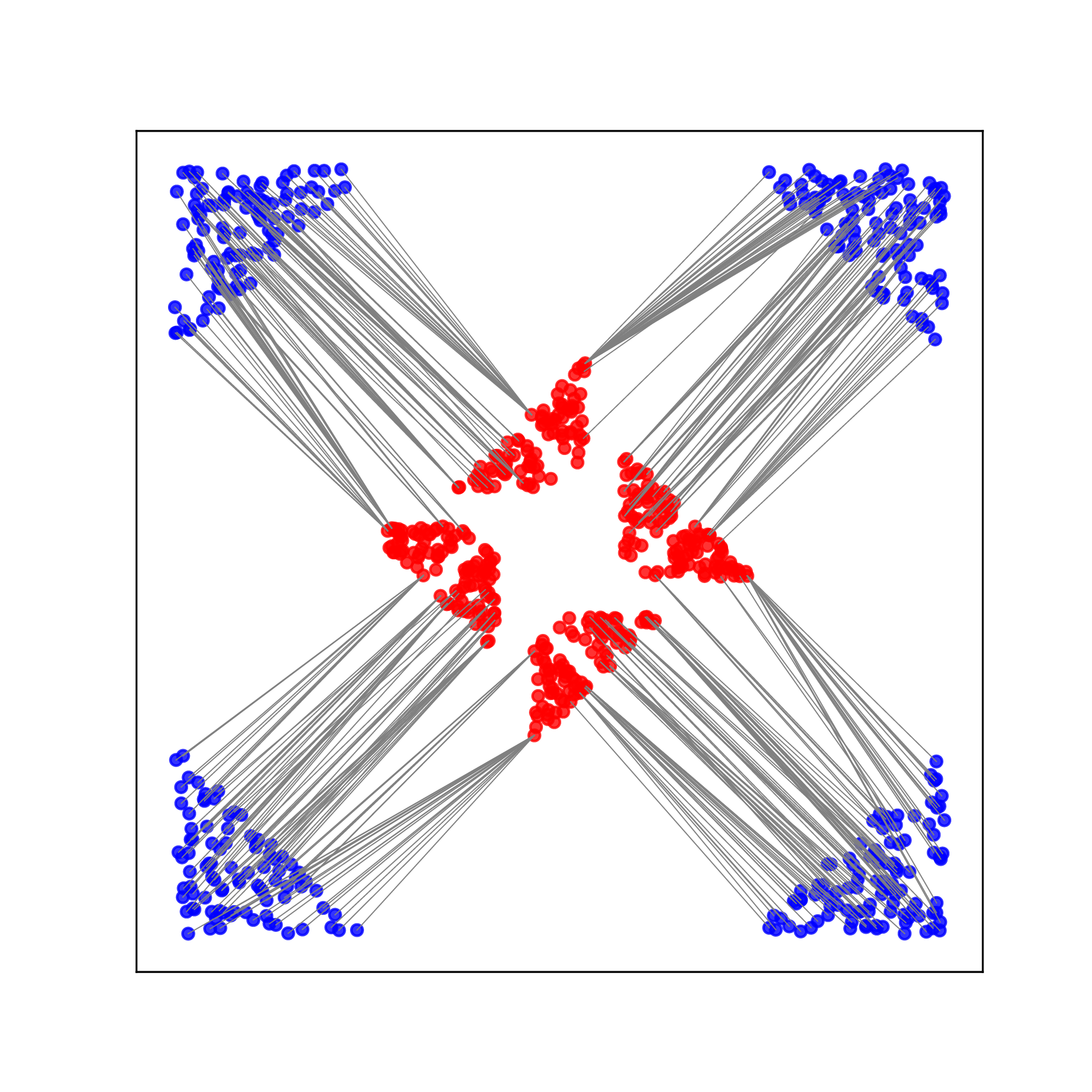
(a) OT 

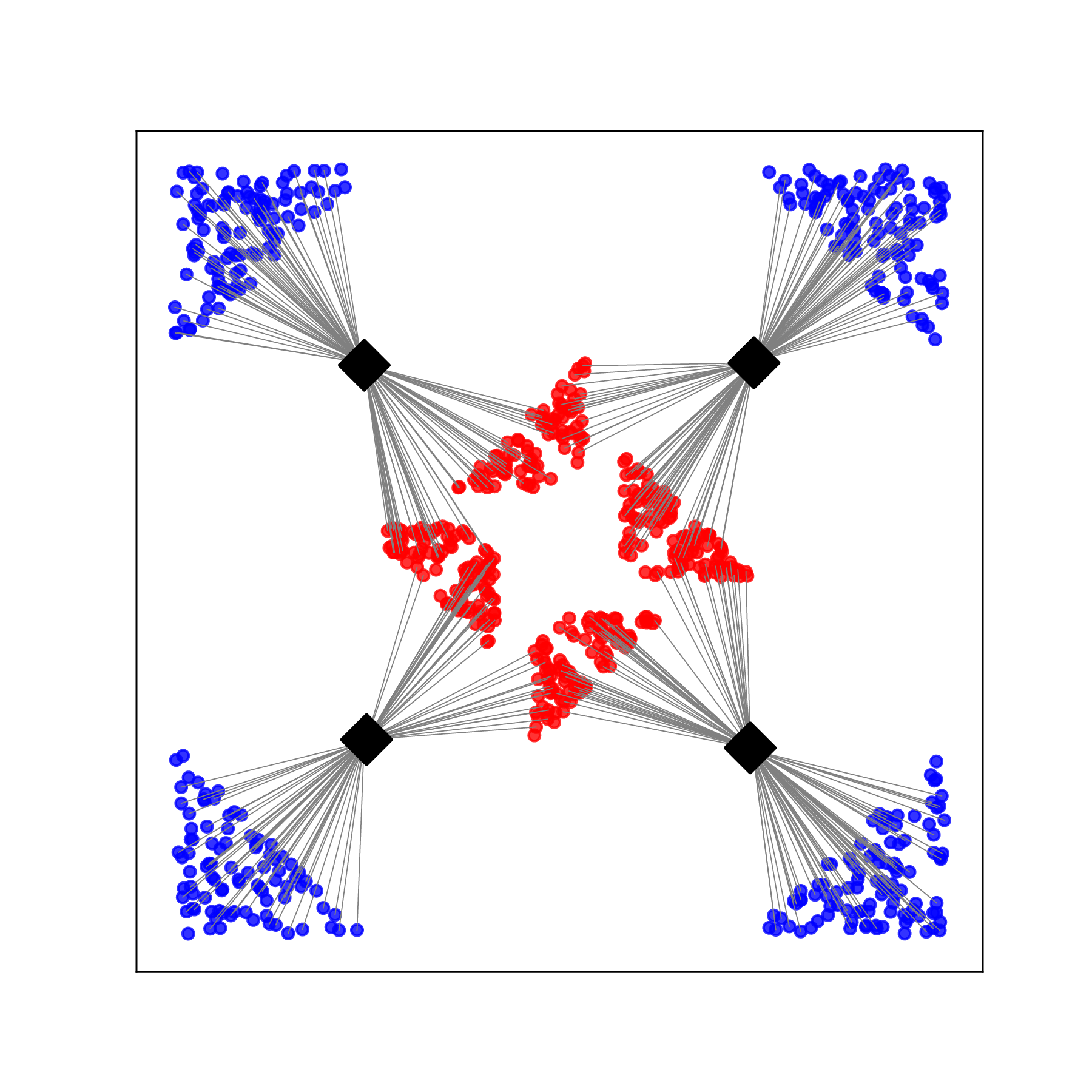
(b) FC 

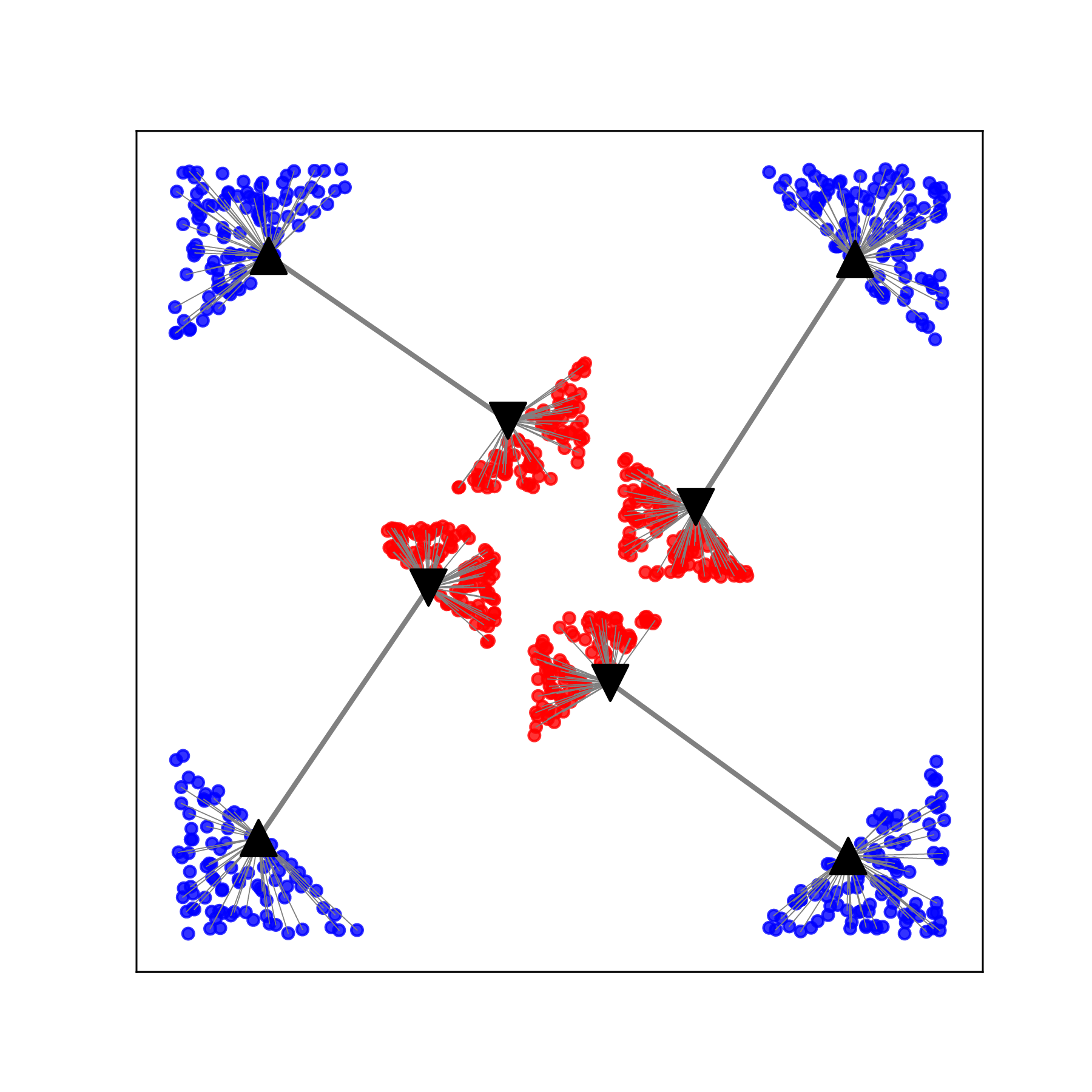
(c) LOT (4,4)

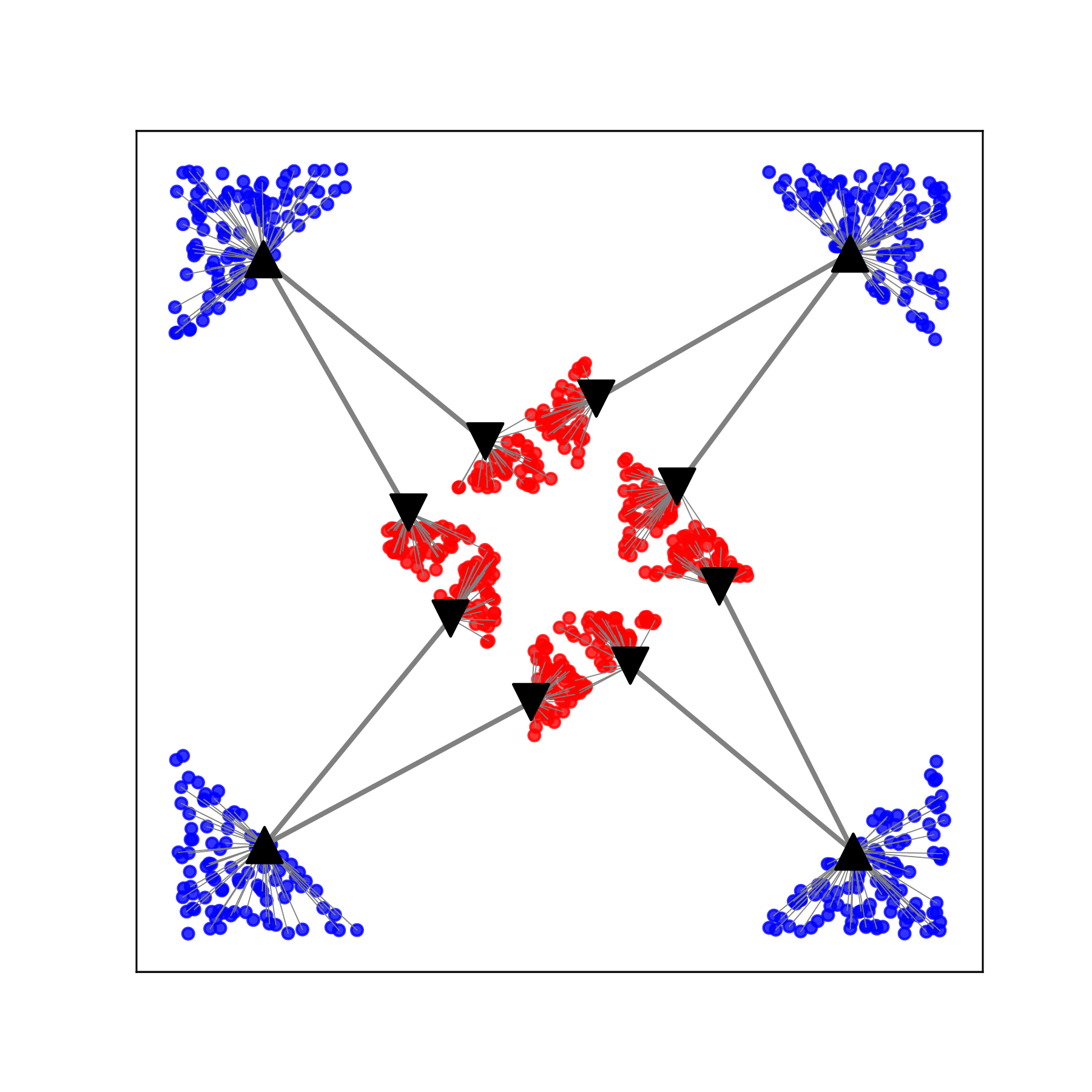
(d) LOT (8,4)

Figure 1: Comparisons of transport plans obtained for different methods applied to clustered data after domain shift. Here, we visualize the connection between the source (blue) $x$ and its estimated target (red) $\hat{y}=\mathop{\textnormal{argmax}}_{y}p(y|x)$. From left to right, we show the standard OT plan (a) and the factored coupling (FC) approach (b). To the right, we show the result of LOT when we use 4 anchors in the target with the same number in the target (c) and 8 anchors in the target (d).

Specifically, our contributions are as follows. (i) We introduce LOT , a new form of structured transport, and propose an efficient algorithm that solves our proposed objective (Section 3), (ii) Theoretically, we show that LOT can be interpreted as a relaxation to OT, and from a statistical point-of-view, it overcomes the curse of dimensionality in terms of the sampling rate (Section 5), (iii) We study the robustness of the approach to noise, sampling, and various data perturbations when applied to both synthetic data and domain adaptation problems in computer vision (Section 6).

2 Background

Optimal Transport:

Optimal transport (OT) (Villani, 2008; Santambrogio, 2015; Peyré et al., 2019) is a distribution alignment technique that learns a transport plan that specifies how to move mass from one distribution to match another. Specifically, consider two sets of data points encoded in matrices, the source $\mathbf{X}=[\mathbf{x}_{1},\dots,\mathbf{x}_{n}]$ and the target $\mathbf{Y}=[\mathbf{y}_{1},\dots,\mathbf{y}_{m}]$, where $\mathbf{x}_{i}\in{\mathcal{X}}$, $\mathbf{y}_{j}\in{\mathcal{Y}}$, $\forall i,j$. Assume they are endowed with discrete measures $\mu=\sum_{i=1}^{N}p(\mathbf{x}_{i})\delta_{\mathbf{x}_{i}}$, $\nu=\sum_{j=1}^{M}p(\mathbf{y}_{j})\delta_{\mathbf{y}_{j}}$, respectively. The cost of transporting $\mathbf{x}_{i}$ to $\mathbf{y}_{j}$ is $c(\mathbf{x}_{i},\mathbf{y}_{j})$, where $c$ denotes some cost function. OT considers the most cost-efficient transport by solving the following problem:

$$\text{OT}_{\mathbf{C}}(\mu,\nu):=\min_{{\mathbf{P}\mathbf{1}}=\mu,{\mathbf{P}}^{T}{\mathbf{1}}=\nu}\langle{\mathbf{C}},{\mathbf{P}}\rangle,$$ (1)

where $\mathbf{P}:=[p(\mathbf{x}_{i},\mathbf{y}_{j})]_{i,j}$ is the source-to-target transport plan matrix (coupling), and ${\mathbf{C}}=[c(\mathbf{x}_{i},\mathbf{y}_{j})]_{i,j}$ is the cost matrix. When $c(\mathbf{x},\mathbf{y})=d(\mathbf{x},\mathbf{y})^{p}$, where $d$ is a distance function, ${\cal{W}}_{p}:=\text{OT}_{\textbf{C}}^{{1}/{p}}$ defines a distance called the $p$-Wasserstein distance. The objective in (1) is a linear programming problem, where computation speed can be prohibitive if $n$ is large (Pele & Werman, 2009). A common speedup is to replace the objective by an entropy-regularized proxy,

$$\text{OT}_{\mathbf{C},\varepsilon}(\mu,\nu): =\min_{{\mathbf{P}\mathbf{1}}=\mu,{\mathbf{P}}^{T}{\mathbf{1}}=\nu}\langle\mathbf{C},{\mathbf{P}}\rangle-\varepsilon\mathbf{H}(\mathbf{P})$$

$$=\min_{{\mathbf{P}\mathbf{1}}=\mu,{\mathbf{P}}^{T}{\mathbf{1}}=\nu}\varepsilon\text{KL}({\bf P}||{\bf K}),$$ (2)

where ${\bf K}$ is the Gibbs kernel induced by the element-wise exponential of the cost matrix $\mathbf{K}:=\exp(-\mathbf{C}/\varepsilon)$, $\mathbf{H}(\mathbf{P}):=-\sum_{ij}\mathbf{P}_{ij}\log(\mathbf{P}_{i,j})$ is the Shannon entropy, and $\varepsilon$ is a user-specified hyperparameter that controls the amount of entropic regularization that is introduced. We can alternatively write the objective function as a minimization of $\varepsilon\text{KL}(\mathbf{P}\|\mathbf{K})$, where KL denotes the Kullback-Leibler divergence. In practice, the entropy-regularized form is often used over the original objective (1) as it admits a fast method called the Sinkhorn algorithm (Cuturi, 2013; Altschuler et al., 2017). Hence, we will use OT to refer to the entropy-regularized form unless specified otherwise in the context.

Optimal Transport via Factored Couplings:  Factored Coupling (FC) is proposed in (Forrow et al., 2019) to reduce the sample complexity of OT in high dimensions. Specifically, it adds an additional constraint to (1) by enforcing the transport plan to be of the following factored form,

$$\vspace{-1mm}p(\mathbf{x}_{i},\mathbf{y}_{j})=\sum_{l=1}^{k}p(\mathbf{z}_{l})p(\mathbf{x}_{i}|\mathbf{z}_{l})p(\mathbf{y}_{j}|\mathbf{z}_{l}).\vspace{-2mm}$$ (3)

This has a nice interpretation: $\mathbf{z}_{l}$ serves as a common “anchor” that transportation from $\mathbf{x}_{i}$ to $\mathbf{y}_{j}$ must pass through. It turns out that FC is closely related to the Wasserstein barycenter problem (Agueh & Carlier, 2011; Cuturi & Doucet, 2014; Cuturi & Peyré, 2016), $\min_{\nu}\sum_{i=1}^{N}{\cal{W}}^{2}_{2}(\mu_{i},\nu)$, where $\nu$ is the Procrustes mean to distributions $\mu_{i}$, $i=1,\dots,N$ with respect to the squared 2-Wasserstein distance. A crucial insight from (Forrow et al., 2019) is that for $N=2$, the barycenter $\nu$ could approximate the optimal anchors to a transport plan of the form (3) that minimizes the objective in (1).

3 Latent Optimal Transport

3.1 Motivation

Most datasets have low-dimensional latent structure, but OT does not naturally use it during transport. This motivates the idea that distribution alignment methods should both reveal the latent structure in the data in addition to aligning these latent structures. An illustrative example is provided in Figure 1; here, we show the transport plan for a source (red points) and a target (blue points), both of which exhibit clear cluster structures. Because OT transports points independently, the points can be easily mapped outside of their original cluster (a). In comparison, low-rank OTs (b-d) induce transport plans that are better at preserving clusters. In (b), because factored coupling (FC) transports points via common anchors (black squares), the anchors need to interpolate between both distributions, and it loses the freedom of choosing different structures for the source and target. On the other hand, by specifying different numbers of anchors for the source and target individually (c vs. d), LOT can extract different structures and output different transport plans.

3.2 Problem formulation

Consider data matrices $\mathbf{X}$ and $\mathbf{Y}$ and their measures $\mu$, $\nu$, as detailed in Section 2. We introduce “anchors” through which points must flow, thus constraining the transportation. The anchors are stacked in data matrices $\mathbf{Z}_{x}:=[\mathbf{z}^{x}_{1},\dots,\mathbf{z}^{x}_{k_{x}}]$, $\mathbf{Z}_{y}:=[\mathbf{z}^{y}_{1},\dots,\mathbf{z}^{y}_{k_{y}}]$. We denote the measures of the source and target anchors as $\mu_{z}=\sum_{m=1}^{k_{x}}p(\mathbf{z}^{x}_{m})\delta_{\mathbf{z}^{x}_{m}}$ and $\nu_{z}=\sum_{n=1}^{k_{y}}p(\mathbf{z}^{y}_{n})\delta_{\mathbf{z}^{y}_{n}}$. For any set ${\cal{A}}$, we further denote $\Delta^{k}_{\cal{A}}:=\left\{\sum_{i=1}^{k}\mathbf{\omega}_{i}\delta_{\mathbf{a}_{i}}:\sum_{i=1}^{k}\mathbf{\omega}_{i}=1,\mathbf{\omega}_{i}\geq 0,\mathbf{a}_{i}\in{\cal{A}},\forall i\right\}$ as the set of probability measures on ${\cal{A}}$ that has discrete support of size up to $k$. Hence $\mu_{z}\in\Delta^{k_{x}}_{{\mathcal{Z}}_{x}}$, $\nu_{z}\in\Delta^{k_{y}}_{{\mathcal{Z}}_{y}}$, where ${\mathcal{Z}}_{x}$ (resp. ${\mathcal{Z}}_{y}$) is the space of source (resp. target) anchors. If we interpret the conditional probability $p(a|b)$ as the strength of transportation from $b$ to $a$, then, using the chain rule, the concurrence probability $p(\mathbf{x}_{i},\mathbf{y}_{j})$ of $\mathbf{x}_{i}$ and $\mathbf{y}_{j}$ can be written as,

$$p(\mathbf{x}_{i},\mathbf{y}_{j})= \sum_{m,n}p(\mathbf{x}_{i})p(\mathbf{z}_{m}^{x}|\mathbf{x}_{i})p(\mathbf{z}^{y}_{n}|\mathbf{z}_{m}^{x})p(\mathbf{y}_{j}|\mathbf{z}^{y}_{n})$$

$$= \sum_{m,n}p(\mathbf{x}_{i},\mathbf{z}_{m}^{x})\frac{p(\mathbf{z}_{m}^{x},\mathbf{z}^{y}_{n})}{p(\mathbf{z}_{m}^{x})p(\mathbf{z}^{y}_{n})}p(\mathbf{z}^{y}_{n},\mathbf{y}_{j}).$$ (4)

When encoding these probabilities using a transport matrix $\mathbf{P}:=[p(\mathbf{x}_{i},\mathbf{y}_{j})]_{i,j}$, the factorized form (3.2) can be written as,

$$\vspace{-1mm}\mathbf{P}=\mathbf{P}_{x}\text{diag}(\mathbf{u}_{z}^{-1})\mathbf{P}_{z}\text{diag}(\mathbf{v}_{z}^{-1})\mathbf{P}_{y},$$ (5)

where $\mathbf{P}_{x}$ encodes transport from source space to source anchor space (i.e., $p(\mathbf{x}_{i},\mathbf{z}^{x}_{m})$), $\mathbf{P}_{z}$ encodes transport from source anchor space to target anchor space, $\mathbf{P}_{y}$ encodes transport from target anchor space to target space , and $\mathbf{u}_{z}:=[p(\mathbf{z}^{x}_{1}),\cdots,p(\mathbf{z}^{x}_{k_{x}})]$, $\mathbf{v}_{z}:=[p(\mathbf{z}^{y}_{1}),\cdots,p(\mathbf{z}^{y}_{k_{y}})]$ encode the latent distributions of anchors. To learn each of these transport plans, we must first designate the ground metric used to define the cost in each of the three stages. The cost matrices $\mathbf{C}_{x},\mathbf{C}_{y}$ determine how points will be transported to their respective anchors and thus dictate how the data structure will be extracted. We will elaborate on the choice of costs in Section 3.3.

We now formalize our proposed approach to transport in the following definition.

Definition 1.

Let $\mathbf{C}_{x}$, $\mathbf{C}_{y}$ denote the cost matrices between the source/target and their representative anchors, and let $\mathbf{C}_{z}$ denote the cost matrix between anchors. We define the latent optimal transport (LOT ) problem as,

$$\rm{OT}^{{L}}(\mu,\nu): =\inf_{\mu_{z}\in\Delta_{{\mathcal{Z}}_{x}}^{k_{x}},\nu_{z}\in\Delta_{{\mathcal{Z}}_{y}}^{k_{y}}}\big{\{}\rm{OT}_{\mathbf{C}_{x}}(\mu,\mu_{z})$$

$$+ \rm{OT}_{\mathbf{C}_{z}}(\mu_{z},\nu_{z})+\rm{OT}_{\mathbf{C}_{y}}(\nu_{z},\nu)\big{\}},\vspace{-3mm}$$

where ${\mathcal{Z}}_{x}$ and ${\mathcal{Z}}_{y}$ are the latent spaces of the source and target anchors, respectively.

The intuition behind Def. 1 is that we use $\rm{OT}_{\mathbf{C}_{x}}(\mu,\mu_{z})$ and $\rm{OT}_{\mathbf{C}_{y}}(\nu_{z},\nu)$ to capture group structure in each space, and then $\rm{OT}_{\mathbf{C}_{z}}(\mu_{z},\nu_{z})$ to align the source and target by determining the transportation across anchors. Hence, LOT can be interpreted as an optimization of joint clustering and alignment. The flexibility of cost matrices allows LOT to capture different structures and induce different transport plans. In Section 5, we further show that LOT can be regarded as a relaxation of an OT problem.

Remark 1.

In Forrow et al. (2019), the authors introduce the notion of the transport rank for a transport plan $\mathbf{P}$ as the minimum number of product probability measures that its corresponding coupling can be composed from, i.e., $p(\mathbf{x},\mathbf{y})=\sum_{i=1}^{r}\lambda_{i}\left(p_{i}(\mathbf{x})\otimes p_{i}(\mathbf{y})\right)$, $\lambda_{i}\geq 0$, $\forall i$. In general, given a transportation plan $\mathbf{P}$, the transport rank ${\rm rank}_{+}(\mathbf{P})$ is lower bounded by its usual matrix rank ${\rm rank}(\mathbf{P})$. In the case of LOT, the transport plan induced by Def. 1 satisfies ${\rm rank}(\mathbf{P})\leq{\rm rank}_{+}(\mathbf{P})\leq\min(k_{x},k_{y})$. Thus, by selecting a small number of anchors we naturally induce a low-rank solution for transport.

Next, we show some properties of LOT that highlight its similarity to a metric.

Proposition 1.

Suppose the latent spaces ${\cal{Z}}_{x}={\cal{Z}}_{y}$ are the same as the original data spaces ${\cal{X}}={\cal{Y}}$, and the cost matrices are defined by $\mathbf{C}_{x}[a,b]=\mathbf{C}_{z}[a,b]=\mathbf{C}_{y}[a,b]=d(a,b)^{p}$, where $p\geq 1$ and $d$ is some distance function. If we define the latent Wasserstein discrepancy as ${\cal{W}}^{L}_{p}:={(\rm{OT}^{L})}^{1/p}$, then there exist $\kappa>0$ such that, for any $\mu$, $\nu$ and $\zeta$ having latent distributions of support sizes up to $k$, the discrepancy satisfies,

• ${\cal{W}}_{p}^{L}(\mu,\nu)\geq 0$

• ${\cal{W}}_{p}^{L}(\mu,\nu)={\cal{W}}_{p}^{L}(\nu,\mu)$

• ${\cal{W}}_{p}^{L}(\mu,\nu)\leq\kappa\left({\cal{W}}_{p}^{L}(\mu,\zeta)+{\cal{W}}_{p}^{L}(\zeta,\nu)\right)$

The low-rank nature of LOT has a biasing effect that results in ${\cal{W}}_{p}^{L}(\mu,\mu)>0$ for a general $\mu$. We can debias it by defining its variant $\tilde{{\cal{W}}}_{p}^{L}(\mu,\nu):=\left(\left({\cal{W}}_{p}^{L}(\mu,\nu)\right)^{p}-\min\limits_{z_{k}\in{\Phi}_{x}}{\cal{W}}_{p}^{p}(\mu,z_{k})-\min\limits_{z^{\prime}_{k}\in{\Phi}_{y}}{\cal{W}}_{p}^{p}(\nu,z^{\prime}_{k})\right)^{1/p}$, where ${{\Phi}}_{x}=\Delta_{{\cal{Z}}_{x}}^{k_{x}}$, ${{\Phi}}_{y}=\Delta_{{\cal{Z}}_{y}}^{k_{y}}$. The following property connects $\tilde{{\cal{W}}}_{p}^{L}(\mu,\nu)$ to k-means clustering.

Corollary 1.

Under the assumptions of Proposition 1, if $p=2$ and $k_{x}=k_{y}=k$, then $\forall\mu,\nu$, we have $\tilde{{\cal{W}}}_{2}^{L}(\mu,\nu)\geq 0$. Furthermore, $\tilde{{\cal{W}}}_{2}^{L}(\mu,\nu)>0$ if their k-means centroids or sizes of their k-means clusters differ.

3.3 Establishing a ground metric

In what follows, we will focus on the Euclidean space ${\cal{X}}={\cal{Y}}=\mathbb{R}^{d}$. Instead of considering every source-to-target distance to build our transportation cost, we can use anchors as proxies for each point. A well-established way of encoding the distance that each point needs to travel to get to its nearest anchor, is to define the cost as:

$$\mathbf{C}_{x}=d_{\mathbf{M}_{x}},\mathbf{C}_{z}=d_{\mathbf{M}_{z}},\mathbf{C}_{y}=d_{\mathbf{M}_{y}},$$ (6)

where $d_{\mathbf{M}}$ denotes the Mahalanobis distance: $d^{2}_{\mathbf{M}}(\mathbf{x},\mathbf{y}):=(\mathbf{x}-\mathbf{y})^{T}{\mathbf{M}}(\mathbf{x}-\mathbf{y})$ and ${\mathbf{M}}$ is some positive semidefinite matrix. The Mahalanobis distance generalizes the squared Euclidean distance and allows us to consider different costs based on correlations between features. The framework of Mahalanobis distance benefits from efficient metric learning techniques (Cuturi & Avis, 2014); recent research also establishes connections between it and robust OT (Paty & Cuturi, 2019; Dhouib et al., 2020). When a simple L2-distance is used ($\mathbf{M}=\mathbf{I}$), we will denote this specific variant as LOT -L2 .

When LOT moves source points through anchors, the anchors impose a type of bottleneck, and this results in a loss of information that makes it difficult to estimate the corresponding point in the target space. In cases where accurate point-to-point alignment is desired, we propose an alternative strategy for defining the cost matrix $\mathbf{C}_{z}$. The idea is to represent an anchor as the distribution of points assigned to it. Specifically, we represent $\mathbf{z}^{x},\mathbf{z}^{y}$ as measures in $\mathbb{R}^{d}$: $\tilde{\mathbf{z}}^{x}=\sum_{i=1}^{N}\mathbf{P}_{x}(\mathbf{x}_{i}|\mathbf{z}^{x})\delta_{\mathbf{x}_{i}},$ $\tilde{\mathbf{z}}^{y}=\sum_{j=1}^{M}\mathbf{P}_{y}(\mathbf{y}_{j}|\mathbf{z}^{y})\delta_{\mathbf{y}_{j}}$. Then we measure the cost between anchors as the squared Wasserstein distance between their respective distributions,

$$\mathbf{C}_{z}:=[{\cal{W}}^{2}_{2}(\mathbf{P}_{x}(\cdot|\mathbf{z}^{x}_{m}),\mathbf{P}_{y}(\cdot|\mathbf{z}^{y}_{n}))]_{m,n}.$$ (7)

Besides the quantity itself, the transport plan returned by calculating $\mathbf{C}_{z}$ is also very important as it provides accurate point-to-point maps. Since the cost matrix is now a function of $\mathbf{P}_{x}$ and $\mathbf{P}_{y}$, we use an additional alternating scheme to solve the problem: we alternate between updating $\mathbf{C}_{z}$ while keeping $\mathbf{P}_{x}$ and $\mathbf{P}_{y}$ fixed, and then updating $\mathbf{P}_{x},\mathbf{P}_{y},\mathbf{P}_{z}$ while keeping $\mathbf{C}_{z}$ fixed. An efficient algorithm is presented in Appendix B.3 to reduce the computation complexity. This variant, LOT -WA , can yield better performance in downstream tasks that require precise alignment at the cost of additional computation.

3.4 Algorithm

In the rest of this section, we will develop our main approach for solving the problem in Def. 1. We provide an outline of the algorithm in Algorithm 1 and an implementation of the algorithm in Python at:  http://nerdslab.github.io/latentOT.

(1) Optimizing $\mathbf{P}_{x},\mathbf{P}_{y}$ and $\mathbf{P}_{z}$:

To begin, we assume that the anchors and cost matrices $\mathbf{C}_{x},\mathbf{C}_{z},\mathbf{C}_{y}$ are already specified. Let $\mathbf{K}_{x},\mathbf{K}_{z},\mathbf{K}_{y}$ be the Gibbs kernels induced from the cost matrices $\mathbf{C}_{x},\mathbf{C}_{z},\mathbf{C}_{y}$ as in (2). The optimization problem can be written as,

$$\min_{\mathbf{u}_{z},\mathbf{v}_{z},\mathbf{P}_{x},\mathbf{P}_{z},\mathbf{P}_{y}} \sum_{i\in\{x,y,z\}}\varepsilon_{i}\text{KL}(\mathbf{P}_{i}\|\mathbf{K}_{i}),$$

subject to: $$\mathbf{P}_{x}\mathbf{1}=\mu,\mathbf{P}^{T}_{x}\mathbf{1}=\mathbf{u}_{z},\mathbf{P}_{z}\mathbf{1}=\mathbf{u}_{z},$$

$$\mathbf{P}_{z}^{T}\mathbf{1}=\mathbf{v}_{z},\mathbf{P}_{y}\mathbf{1}=\mathbf{v}_{z},\mathbf{P}^{T}_{y}\mathbf{1}=\nu.$$ (8)

This is a Bregman projection problem with affine constraints. An iterative projection procedure can thus be applied to solve the problem (Benamou et al., 2015). We present the procedure as UpdatePlan in Algorithm 1, where $\mathbf{P}_{x},\mathbf{P}_{z},\mathbf{P}_{y}$ are successively projected onto the constrained sets of fixed marginal distributions. We defer the detailed derivation to Appendix B.1.

0:  Data matrices $\mathbf{X}$, $\mathbf{Y}$; metric costs ${\bf M}_{x},{\bf M}_{y},{\bf M}_{z}$; entropy regularization parameters $\varepsilon_{x}$, $\varepsilon_{y}$, $\varepsilon_{z}$; initial anchors $\mathbf{Z}_{x},\mathbf{Z}_{y}$.

0:  Transport plans $\mathbf{P}_{x},\mathbf{P}_{y},\mathbf{P}_{z}$; source and target anchors $\mathbf{Z}_{x}$, $\mathbf{Z}_{y}$.

0:  $\mathbf{P}_{x},\mathbf{P}_{y},\mathbf{P}_{z},\mathbf{Z}_{x},\mathbf{Z}_{y}$

1:  while not converging do

2:     $(\text{vec}(\mathbf{Z}_{x}),\text{vec}(\mathbf{Z}_{y}))\leftarrow$ Eqn. (9)

3:     $\mathbf{K}_{x}=\{\exp(-\|\mathbf{X}[i]-\mathbf{Z}_{x}[j]\|_{\mathbf{M}_{x}}^{2}/\varepsilon_{x})\}_{i,j}$

4:     $\mathbf{K}_{y}=\{\exp(-\|\mathbf{Y}[i]-\mathbf{Z}_{y}[j]\|_{\mathbf{M}_{y}}^{2}/\varepsilon_{y})\}_{j,q}$

5:     $\mathbf{K}_{z}=\{\exp(-\|\mathbf{Z}_{x}[i]-\mathbf{Z}_{y}[j]\|_{\mathbf{M}_{z}}^{2}/\varepsilon_{z})\}_{p,q}$

6:     $\mathbf{P}_{x},\mathbf{P}_{y},\mathbf{P}_{z}\leftarrow$UpdatePlan ($\mathbf{K}_{x},\mathbf{K}_{y},\mathbf{K}_{z}$)

7:  end while

7:  ${\bf P}_{x}$, ${\bf P}_{y}$, ${\bf P}_{z}$, ${\bf Z}_{x}$, ${\bf Z}_{y}$

Algorithm 1 Latent Optimal Transport (LOT)

UpdatePlan ($\mathbf{K}_{x},\mathbf{K}_{y},\mathbf{K}_{z}$)

0:  $\mathbf{\alpha}_{x}\leftarrow\mathbf{1}_{N};\mathbf{\beta}_{x}\leftarrow\mathbf{1}_{k_{1}};\mathbf{\alpha}_{y}\leftarrow\mathbf{1}_{k_{2}}$;      $\mathbf{\beta}_{y}\leftarrow\mathbf{1}_{M};\mathbf{\alpha}_{z}\leftarrow\mathbf{1}_{k_{1}};\mathbf{\beta}_{z}\leftarrow\mathbf{1}_{k_{2}}$

1:  while not converging do

2:     $\alpha_{x}\leftarrow\mu\oslash\mathbf{K}_{x}\beta_{x}$; $\beta_{y}\leftarrow\nu\oslash\mathbf{K}_{y}^{T}\alpha_{y}$

3:     $\mathbf{u}_{z}\leftarrow((\alpha_{z}\odot\mathbf{K}_{z}\beta_{z})\odot(\beta_{x}\odot\mathbf{K}_{x}^{T}\alpha_{x}))^{\frac{1}{2}}$

4:     $\beta_{x}\leftarrow\mathbf{u}_{z}\oslash\mathbf{K}_{x}^{T}\alpha_{x}$; $\alpha_{z}\leftarrow\mathbf{u}_{z}\oslash\mathbf{K}_{z}\beta_{z}$

5:     $\mathbf{v}_{z}\leftarrow((\alpha_{y}\odot\mathbf{K}_{y}\beta_{y})\odot(\beta_{z}\odot\mathbf{K}_{z}^{T}\alpha_{z}))^{\frac{1}{2}}$

6:     $\beta_{z}\leftarrow\mathbf{v}_{z}\oslash\mathbf{K}_{z}^{T}\alpha_{z}$; $\alpha_{y}\leftarrow\mathbf{v}_{z}\oslash\mathbf{K}_{y}\beta_{y}$

7:  end while

7:  $\mathbf{P}_{i}={\text{diag}}(\alpha_{i})\mathbf{K}_{i}{\text{diag}}(\beta_{i})$, $i\in\{x,y,z\}$

Algorithm 1    Latent Optimal Transport - LOT 

(2) Optimizing the anchor locations:

Now we consider the case where we are free to select the anchor locations in $\mathbb{R}^{d}$. We consider the class of Mahalanobis costs described in Section 3.3. Let ${\mathbf{M}}_{x}$, ${\mathbf{M}}_{z}$, ${\mathbf{M}}_{y}$ be the Mahalanobis matrices correspond to $\mathbf{C}_{x}$, $\mathbf{C}_{z}$, and $\mathbf{C}_{y}$, respectively.

Given the transport plans generated after solving (3.4), we can derive the the first-order stationary condition of OT^L with respect to $\mathbf{Z}_{x}$ and $\mathbf{Z}_{y}$. Let

$${\bf A}=\begin{bmatrix}D(\mathbf{u}_{z})\otimes(\mathbf{M}_{x}+\mathbf{M}_{z})&\mathbf{P}_{z}\otimes\mathbf{M}_{z}\\ -\mathbf{P}_{z}^{T}\otimes\mathbf{M}_{z}&D(\mathbf{v}_{z})\otimes(\mathbf{M}_{y}+\mathbf{M}_{z})\end{bmatrix}$$

The update formula is given by

$$\begin{bmatrix}\text{vec}(\mathbf{Z}_{x}^{*})\\ \text{vec}(\textbf{Z}_{y}^{*})\end{bmatrix}={\bf A}^{-1}\times\begin{bmatrix}(\mathbf{P}_{x}^{T}\otimes\mathbf{M}_{x})\text{vec}(\mathbf{X})\\ (\mathbf{P}_{y}\otimes\mathbf{M}_{y})\text{vec}(\mathbf{Y})\end{bmatrix},$$ (9)

where $\text{vec}(\cdot)$ denotes the operator converting a matrix to a column vector, and $D(\cdot)$ denotes the operator converting a vector to a diagonal matrix. We defer the detailed derivation to Appendix B.2. Pseudo-code for the combined scheme can be found in Algorithm 1.

(3) Robust estimation of data transport:

LOT provides robust transport in the target domain by aligning the data through anchors, which can facilitate regression, and classification in downstream applications. We denote the centroids of the source and target by $\mathbf{Q}_{x}=\text{diag}(\mathbf{u}_{z}^{-1})\mathbf{P}_{x}^{T}\mathbf{X}^{T}$, $\mathbf{Q}_{y}=\text{diag}(\mathbf{v}_{z}^{-1})\mathbf{P}_{y}\mathbf{Y}^{T}$. We propose the estimator $\hat{\mathbf{X}}:=\sum_{m,n}p(\mathbf{z}_{m}^{x},\mathbf{z}_{n}^{y}|\mathbf{x})(\mathbf{Q}^{y}_{m}-\mathbf{Q}^{x}_{n})=\text{diag}(\mu^{-1})\mathbf{P}_{x}\text{diag}((\mathbf{P}_{z}\mathbf{1})^{-1})\mathbf{P}_{z}(\mathbf{Q}_{y}-\mathbf{Q}_{x}).$ In contrast to factored coupling (Forrow et al., 2019), where $\mathbf{Z}_{x}=\mathbf{Z}_{y}$, LOT is robust even when the source and target have different structures (see Table 1 MNIST-DU, Figure 5).

(4) Implementation details:

LOT has two primary hyperparameters that must be specified: (i) the number of the source and target anchors $k_{x},k_{y}$ and (ii) the regularization parameter $\varepsilon$. For details on the tuning of these parameters, please refer to Appendix F. In practice, we use centroids from k-means clustering (Arthur & Vassilvitskii, 2006) to initialize the anchors, and for all the experiments we have conducted, LOT typically converges within $20$ iterations.

4 Related Work

Interpolation between factored coupling and k-means clustering:  Assume we select the Mahalanobis matrices of the costs defined in Section 3.3 to be $\mathbf{M}_{x}=\mathbf{M}_{y}=\mathbf{I},$ and $\mathbf{M}_{z}=\lambda\mathbf{I}$. If we let $\lambda\to\infty$ when estimating the transport between source and target anchors, the anchors merge, and our approach reduces to the case of factored coupling (Forrow et al., 2019). At the other end, if we let $\lambda\to 0$, then LOT becomes separable, and the middle term vanishes. In this case, each remaining term exactly corresponds to a pure clustering task, and LOT reduces to k-means clustering (Arthur & Vassilvitskii, 2006).

Relationship to OT -based clustering methods:  Many methods that combine OT and clustering (Li & Wang, 2008; Ye et al., 2017; Ho et al., 2017; Dessein et al., 2017; Genevay et al., 2019; Alvarez-Melis & Fusi, 2020) focus on using the Wasserstein distance to identify barycenters that serve as the centroids of clusters. When finding barycenters for the source and target separately, this could be seen as LOT with $\mathbf{C}_{z}=0$ and $\mathbf{C}_{x}$, $\mathbf{C}_{y}$ defined using a squared L2 distance. In other related work (Laclau et al., 2017), co-clustering is applied to a transport plan as a post-processing operation, and no additional regularization on the transportation cost in OT is imposed. In contrast, our approach induces explicit regularization by separately defining cost matrices for the transport between the source/target points and their anchors. This yields a transport plan guided by a cluster-level matching.

Relationship to hierarchical OT :  Hierarchical OT (Chen et al., 2018; Lee et al., 2019; Yurochkin et al., 2019; Xu et al., 2020) transports points by moving them within some predetermined subgroup simultaneously based on either their class label or pre-specified structures, and then forms a matching of these subgroups using the Wasserstein distance. The resulting problem solves a multi-layer OT problem which gives rise to its name. With a Wasserstein distance used to build the $\mathbf{C}_{z}$ cost matrix, LOT effectively reduces to hierarchical OT for fixed and hard-class assignment $\mathbf{P}_{x}$ and $\mathbf{P}_{y}$. However, a crucial difference between LOT and hierarchical OT lies in that the latter imposes the known structure information. In contrast, LOT discovers this structure by simultaneously learning $\mathbf{P}_{x}$ and $\mathbf{P}_{y}$.

Transportation with anchors:  The notion of moving data points with anchors to match points in heterogeneous spaces has appeared in other work (Sato et al., 2020; Manay et al., 2006). These approaches map each point from one domain into a distribution of the costs, which effectively builds up a common representation for the points from both spaces. In contrast to this work, we use the anchors to encourage clustering of data and to impose rank constraints on the transport plan.

5 Theoretical Analysis

LOT as a relaxation of OT:  We now ask how the optimal value of our original rank-constrained objective in (3.4) is related to the transportation cost defined in entropy-regularized OT. It turns out their objectives are connected by an inequality described below (see Appendix A for a proof).

Proposition 2.

Let $\bf P$ be a transport plan of the form in (5). Assume that $\mathbf{K}$ is some Gibbs kernel that satisfies,

$$\mathbf{K}_{x}\mathbf{K}_{z}\mathbf{K}_{y}\leq\mathbf{K},$$ (10)

where the inequality is over each entry. Then we have,

$$\varepsilon\text{KL}(\mathbf{P}\|\mathbf{K})\leq \varepsilon(\text{KL}(\mathbf{P}_{x}\|\mathbf{K}_{x})+\text{KL}(\mathbf{P}_{z}\|\mathbf{K}_{z})$$

$$+ \text{KL}(\mathbf{P}_{y}\|\mathbf{K}_{y}))+\varepsilon(\mathbf{H}(\mathbf{u}_{z})+\mathbf{H}(\mathbf{v}_{z})),$$ (11)

where $\mathbf{H}(\mathbf{a}):=-\sum_{i}\mathbf{a}_{i}\log\mathbf{a}_{i}$ denotes the entropy.

The proposition shows that an OT objective, corresponding to a kernel $\mathbf{K}$ (resp. $\mathbf{C}$), can be upper bounded by three sub-OT problems defined by subsequent kernels $\mathbf{K}_{x},\mathbf{K}_{z},\mathbf{K}_{y}$ (resp. $\mathbf{C}_{x},\mathbf{C}_{z},\mathbf{C}_{y}$) that satisfies (10) (resp. $\exp(-\mathbf{C}_{x}/\varepsilon)\exp(-\mathbf{C}_{z}/\varepsilon)\exp(-\mathbf{C}_{y}/\varepsilon)\leq\exp(-\mathbf{C}/\varepsilon)$).

Let us compare the upper bound given by Proposition 2 with Def. 1 and ignore the entropy terms; we recognize that it is precisely the entropy-regularized objective of LOT . In other words, with suitable cost matrices satisfying (10), LOT could be interpreted as a relaxation of an OT problem in a decomposed form. We then ask what $\mathbf{C}_{x}$, $\mathbf{C}_{z}$, $\mathbf{C}_{y}$ should be to satisfy (10). In cases where cost $\mathbf{C}$ is defined by the $L^{p}$-norm to the power $p$, the following corollary shows that the same form suffices.

Corollary 2.

Let $d(\mathbf{x},\mathbf{y}):=\|\mathbf{x}-\mathbf{y}\|_{p}^{p}$. Consider an optimal transport problem OT_C,ε with cost $\mathbf{C}[i,j]=d(\mathbf{x}_{i},\mathbf{y}_{j})$, where $p\geq 1$. Then for a sufficiently small $\varepsilon$, the latent optimal transport OT^L with cost matrices, $\mathbf{C}_{x}[i,m]=3^{p-1}d(\mathbf{x}_{i}-\mathbf{z}^{x}_{m}),\mathbf{C}_{z}[m,n]=3^{p-1}d(\mathbf{z}^{x}_{m}-\mathbf{z}^{y}_{n}),\mathbf{C}_{y}[n,j]=3^{p-1}d(\mathbf{z}^{y}_{n}-\mathbf{y}_{j})$ minimizes an upper bound of the entropy-regularized OT objective in (2).

Corollary (2) provides natural costs for LOT to be posed as a relaxation to a OT problem with $L^{p}$ norm. More generally, finding the optimal cost functions that obey (10) and minimize the gap in the inequality in Proposition 2 is outside the scope of this work but would be an interesting topic for future investigation.

(a)

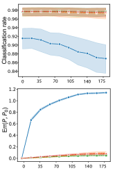
(a) Rotation angle

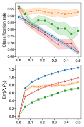
(b) Outlier rate

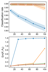
(c) Dimensionality

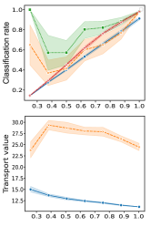
(d) Cluster mismatch

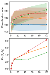
(e) Transport rank

Figure 2: Results on Gaussian mixture models. In (a), we apply a rotation between the source and target, in (b) we add outliers, in (c) we vary the ambient dimension, in (d) the target is set to have $8$ components, and we vary the number of components in the source to simulate source-target mismatch, in (e) we fix the rank to 10 and vary the number of factors (anchors) used in the approximation. Throughout, we simulate data according to a GMM and evaluate performance by measuring the classification accuracy (top) and computing the deviation between the transport plans before and after the perturbations with respect to the Fröbenius norm (bottom).

Sampling complexity:  Below we analyze LOT from a statistical point of view. Specifically, we bound the sampling rate of $\rm{OT}^{L}$ in Def. 1 when the true distributions $\mu$ and $\nu$ are estimated by their empirical distributions.

Proposition 3.

Suppose $X$ and $Y$ have distributions $\mu$ and $\nu$ supported on a compact region $\Omega$ in $\mathbb{R}^{d}$, the cost functions $c_{x}(\cdot,\cdot)$ and $c_{y}(\cdot,\cdot)$ are defined as the squared Euclidean distance, and $\hat{\mu}$, $\hat{\nu}$ are empirical distributions of $n$ and $m$ i.i.d. samples from $\mu$ and $\nu$, respectively. If the spaces for latent distributions are equal to ${\cal{Z}}_{x}={\cal{Z}}_{y}=\mathbb{R}^{d}$, and there are $k_{x}$ and $k_{y}$ anchors in the source and target, respectively, then with probability at least $1-\delta$,

$${\rm Err}\leavevmode\nobreak\ \leq\leavevmode\nobreak\ C\sqrt{\frac{k_{max}^{3}d\log k_{max}+\log(2/\delta)}{N}},$$ (12)

where ${\rm Err}=|{\rm OT}^{L}(\mu,\nu)-{\rm OT}^{L}(\hat{\mu},\hat{\nu})|$, $k_{max}=\max\{k_{x},k_{y}\}$, $N=\min\{n,m\}$ and $C\geq 0$ is some constant not depending on $N$.

As shown in (Weed et al., 2019), the general sampling rate of a plug-in OT scales with $N^{\frac{1}{d}}$, suffering from the “curse of dimensionality”. On the other hand, as evidence from (Forrow et al., 2019), structural optimal transport paves ways to overcome the issue. In particular, LOT achieves $N^{-\frac{1}{2}}$ scaling by regularizing the transport rank.

Time complexity: We can bound the time complexity as $O(T_{\rm i}+T_{\rm{bcd}}(T_{\rm k}+T_{\rm au}+T_{\rm pu}))$, where $T_{\rm i}$ is the initialization complexity, e.g., if we use k-means, then it equals to $O(nk_{x}dT_{x}+mk_{y}dT_{y})$ where $T_{x}$ and $T_{y}$ are the iteration numbers of the Floyd algorithm applied to the source and target, respectively, $T_{\rm bcd}$ is the total number of iterations of block-coordinate descent, $T_{\rm k}=O(nk_{x}+mk_{y})$ is the computation time for updating the kernels, $T_{\rm au}=O((k_{x}+k_{y})^{3}+d(nk_{x}+mk_{y}))$ is the complexity of updating anchors, and $T_{\rm pu}$ is the complexity for updating plans. Because our updates are based on iterative Bregman projections similar to the Sinkhorn algorithm, it has complexity comparable to OT. Therefore, the overall complexity of LOT is approximately $T_{\rm bcd}$ times of OT, assuming $n,\leavevmode\nobreak\ m\geq d(k_{x}+k_{y})$. Empirically, $T_{\rm bcd}$ depends on the structure of data, but we observed that it is usually under $20$. Note that the same applies to FC with $k_{x}=k_{y}=k$. In Figure 3, we complement our analysis by simulating a comparison of the time complexity for LOT and FC vs. OT in the setting of a 7-component Gaussian mixture model. We can see the compute time of LOT scales similarly to FC.

Transport cost:

We also compare the transport loss returned by LOT (blue), FC (orange), and OT (green) as a function of the number of anchors in Figure 3. For a fair comparison, we considered a balanced scenario where 7-component GMMs generate the source and target. The anchors of the source and target are chosen to be equal for LOT . The result shows that the losses are indeed higher for LOT and FC compared to OT but are fairly insensitive with to the chosen number of anchors. Moreover, we find that LOT has a slightly lower loss compared to FC even when we choose the number of source and target anchors to be equal.

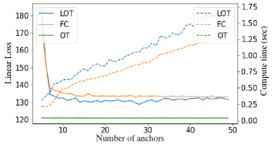
(a)

Figure 3: Comparisons of the time complexity and loss. The figure compares the time complexity (dashed) and linear loss (solid) of LOT, FC, and OT in the setting of the 7-component GMM model.

6 Experiments

In this section, we conduct empirical investigations. Details of hyperparameter tuning can be found in Appendix F.

E1) Testing robustness to various data perturbations: To better understand how different types of domain shift impact the transport plans generated by our approach, we considered different transformations between the source and target. To create synthetic data for this task, we generated multiple clusters/components using a k-dimensional Gaussian with random mean and covariance sampled from a Wishart distribution, randomly projected to a 5-dimensional subspace. The source and target are generated independently: we randomly sample a fixed number of points according to the true distribution for each cluster. We compared the performance of the LOT variants proposed in Section 3.3: LOT -L2 (orange curves) and LOT -WA (green curves) with baselines OT (blue curves) and rank regularized factored coupling (FC ) (Graf & Luschgy, 2007) (red curves) in terms of their (i) classification rates and (ii) deviation from the original transport plan without perturbations, which we compute as $\text{Err}({\bf P}-{\bf P}_{0})=\|{\bf P}-{\bf P}_{0}\|_{F}/\|{\bf P}_{0}\|_{F}$, where ${\bf P}_{0}$ is the transport plan obtained before perturbations. The results are averaged over 20 runs, and a 75% confidence interval is used. See Appendix E for further details.

When compared with OT, both our method and FC provide more stable class recovery, even with significant amounts of perturbations (Figure 2). When we examine the error term in the transport plan, we observe that, in most cases, the OT plan deviates rapidly, even for small amounts of perturbations. Both FC and LOT appear to have similar performances across rotations while OT’s performance decreases quickly. In experiment (b), we found that both LOT variants provide substantial improvements on classification subject to outliers, implying the applicability of LOT for noisy data. In experiment (c), we study LOT in the high-dimensional setting; we find that LOT -WA behaves similarly to FC with some degradation in performance after the dimension increases beyond $70$. Next, in experiment (d), we fix the number of components in the target to be $10$, while varying the number in the source from 4 to 10. In contrast to the outlier experiment in (b), LOT -WA shows more resilience to mismatches between the source and target. At the bottom of plot (d), we show the 2-Wasserstein distance (blue) and latent Wasserstein discrepancy (orange) defined in Proposition 1. This shows that the latent Wasserstein discrepancy does indeed provide an upper bound on the 2-Wasserstein distance. Finally, we look at the effect of transport rank on LOT and FC in (e). The plot shows that the slope for LOT is flatter than FC while maintaining similar performances.

E2) Domain adaptation application: In our next experiment, we used LOT to correct for domain shift in a neural network that is trained on one dataset but underperforms on a new but similar dataset (Table 1, Figure 5). MNIST and USPS are two handwritten digits datasets that are semantically similar but that have different pixel-level distributions and thus introduce domain shift (Figure 5a). We train a multi-layer perceptron (MLP) on the training set of the MNIST dataset, freeze the network, and use it for the remaining experiments. The classifier achieves 100% training accuracy and a 98% validation accuracy on MNIST but only achieves 79.3% accuracy on the USPS validation set. We project MNIST’s training samples in the classifier’s output space (logits) and consider the 10D projection to be the target distribution. Similarly, we project images from the USPS dataset in the network’s output space to get our source distribution. We study the performance of LOT in correcting the classifier’s outputs and compare with FC , k-means OT (KOT ) (Forrow et al., 2019), and subspace alignment (SA) (Fernando et al., 2013).

In Table 1, we summarize the results of our comparisons on the domain adaptation task (MNIST-USPS). Our results suggest that both FC and LOT perform pretty well on this task, with LOT beating FC by 2% in terms of their final classification accuracy. We also show that LOT does better than naive KOT . In Figure 5a, we use Isomap to project the distribution of USPS images as well as the alignment results for LOT , FC , and OT. For both LOT and FC , we also display the anchors; note that for LOT , we have two different sets of anchors (source, red; target, blue). This example highlights the alignment of the anchors in our approach and contrasts it with that of FC .

Table 1: Results for concept drift and domain adaptation for handwritten digits. The classification accuracy and L2-error are computed after transport for MNIST to USPS (left) and coarse dropout (right). Our method is compared with the accuracy before alignment (Original), entropy-regularized OT, k-means plus OT (KOT  ), and subspace alignment (SA).

	MNIST-USPS	MNIST-DU
	Accuracy	Accuracy	L2 error
Original	79.3	72.6	0.72
OT	76.9	61.5	0.71
KOT	79.4	60.9	0.73
SA	81.3	72.3	-
FC	84.1	67.2	0.59
LOT -WA	86.2	77.7	0.56

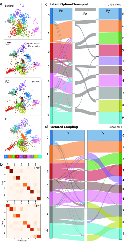
(a)

Figure 5: Visualization of results on handwritten digits and examples of domain shift. (a) 2D projections of representations formed in deep neural network before (top) and after different alignment methods (LOT , FC , OT). (b) confusion matrices for LOT (top) and FC (bottom) after alignment. The transport plans are visualized for LOT (c) and FC (d) in the unbalanced case.

Taking inspiration from studies in self-supervised learning (Doersch et al., 2015; He et al., 2020) that use different transformations of an input image (e.g., masking parts of the image) to build invariances into a network’s representations, here we ask how augmentations of the images introduce domain shift and whether our approach can correct/identify it. To test this, we apply coarse dropout on test samples in MNIST and feed them to the classifier to get a new source distribution. We do this in a balanced (all digits in source and target) and an unbalanced setting (2, 4, 8 removed from source, all digits in target). The results of the unbalanced dropout are summarized in Table 1 (MNIST-DU), and the other results are provided in Table S1 in the Appendix. In this case, we have the features of the testing samples pre-transformation, and thus, we can compare the transported features to the ground truth features in terms of their point-to-point error (L2 distance). In the unbalanced case, we observe even more significant gaps between FC and LOT , as the source and target datasets have different structures. To quantify these different class-level errors, we compare the confusion matrices for the classifier’s output after alignment (Figure 5b). By examining the columns corresponding to the removed digits, we see that FC is more likely to misclassify these images. Our results suggest that LOT has comparable performance with FC in a balanced setting and outperforms FC in an unbalanced case.

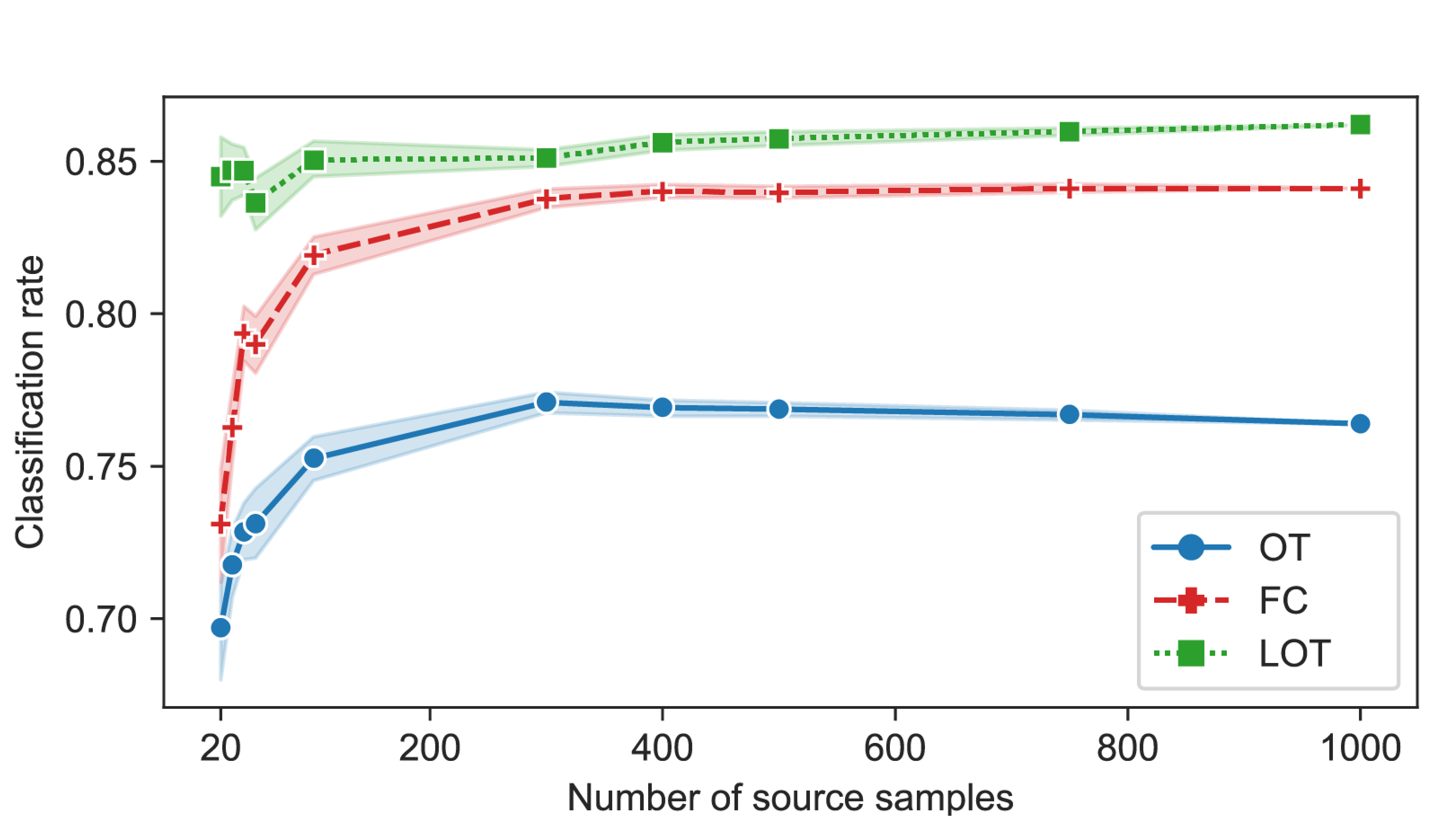
(a)

Figure 6: LOT provides robust alignment, even when given very few samples. We compare our method with OT and FC on the MNIST-USPS domain adaptation task when different numbers of USPS samples are available. Reported classification rates are averaged over 50 random sets.

The decomposition in both LOT and FC allows us to visualize transport between the source, anchors, and the target (Figure 5c-d, S3). This visualization highlights the interpretability of the transport plans learned via our approach, with the middle transport plan ${\bf P}_{z}$ providing a concise map of interactions between class manifolds in the unbalanced setting. With LOT (Figure 5c), we find that each source anchor is mapped to the correct target anchor, with some minor interactions with the target anchors corresponding to the removed digits. In comparison, FC (Figure 5d, S3) has more spurious interactions between source, anchors, and target.

E3) Robustness to sampling: We examined the robustness to sampling for the MNIST to USPS example (Figure 6). In this case, we find that LOT has a stable alignment as we subsample the source dataset, with very little degradation in classification accuracy, even as we reduce the source to only 20 samples. We also observe a significant gap between LOT and other approaches in this experiment, with more than a 10% gap between FC and LOT when very few source samples are provided. Our results demonstrate that LOT is robust to subsampling, providing empirical evidence for Proposition 3.

7 Discussion

In this paper, we introduced LOT , a new form of structured transport leading to an approach for jointly clustering and aligning data. We provided an efficient optimization method to solve for the transport, and studied its statistical rate via theoretical analysis and robustness to data perturbations with empirical experiments. In the future, we would like to explore the application of LOT to non-Euclidean spaces, and incorporate metric learning into our framework.

Appendix

Appendix A Detailed proofs

A.1 Proof of Proposition 1

Proposition 1.

Suppose the latent spaces ${\cal{Z}}_{x}={\cal{Z}}_{y}$ are the same as the original data spaces ${\cal{X}}={\cal{Y}}$, and the cost matrices are defined by $\mathbf{C}_{x}[a,b]=\mathbf{C}_{z}[a,b]=\mathbf{C}_{y}[a,b]=d(a,b)^{p}$, where $p\geq 1$ and $d$ is some distance function. If we define the latent Wasserstein discrepancy as ${\cal{W}}^{L}_{p}:={(\rm{OT}^{L})}^{1/p}$, then there exist $\kappa>0$ such that, for any $\mu$, $\nu$ and $\zeta$ having latent distributions of support sizes up to $k$, the discrepancy satisfies,

• ${\cal{W}}_{p}^{L}(\mu,\nu)\geq 0,$ (Non-negativity)

• ${\cal{W}}_{p}^{L}(\mu,\nu)={\cal{W}}_{p}^{L}(\nu,\mu),$ (Symmetry)

• $\exists\kappa>0$ such that ${\cal{W}}_{p}^{L}(\mu,\nu)\leq\kappa\left({\cal{W}}_{p}^{L}(\mu,\zeta)+{\cal{W}}_{p}^{L}(\zeta,\nu)\right),$ (Quasi-Triangle inequality)

Proof.

The first two properties are easy to verify by non-negativity and symmetry of the Wasserstein distance. Hence we will prove the last property. For brevity, we denote ${\cal{Z}}={\cal{Z}}_{x}={\cal{Z}}_{y}$. Under the assumptions on the cost matrices, we have ${\rm OT}_{\mathbf{C}}={\cal{W}}^{p}_{p}$. Hence there exist latent distributions $\mu_{z}^{*},\zeta_{z}^{*},\zeta_{z}^{\prime*},\nu_{z}^{*}\in\Delta^{k}_{{\cal{Z}}}$ satisfy,

$${(\rm{OT}^{L})}(\mu,\zeta) ={\cal{W}}^{p}_{p}(\mu,\mu_{z}^{*})+{\cal{W}}^{p}_{p}(\mu_{z}^{*},\zeta_{z}^{*})+{\cal{W}}^{p}_{p}(\zeta_{z}^{*},\zeta),$$

$${(\rm{OT}^{L})}(\zeta,\nu) ={\cal{W}}^{p}_{p}(\zeta,{\zeta^{\prime}}^{*}_{z})+{\cal{W}}^{p}_{p}({\zeta^{\prime}}^{*}_{z},\nu_{z}^{*})+{\cal{W}}^{p}_{p}(\nu_{z}^{*},\nu).$$

As $d$ is a distance function, we know that ${\cal{W}}_{p}$ is a metric (Peyré et al., 2019) that satisfies the triangle inequality:

$${\cal{W}}_{p}(\mu,\zeta_{z}^{\prime*})\leq{\cal{W}}_{p}(\mu,\mu_{z}^{*})+{\cal{W}}_{p}(\mu_{z}^{*},\zeta_{z}^{*})+{\cal{W}}_{p}(\zeta^{*}_{z},\zeta)+{\cal{W}}_{p}(\zeta,{\zeta^{\prime}}^{*}_{z}).$$ (13)

On the other hand, Jensen’s inequality tells us that $(a+b+c+d)^{p}\leq 4^{p-1}(a^{p}+b^{p}+c^{p}+d^{p})$ for any non-negative $a,b,c,d$. We apply this inequality to (13) and get,

$${\cal{W}}^{p}_{p}(\mu,{\zeta^{\prime}}^{*}_{z})\leq 4^{p-1}({\cal{W}}^{p}_{p}(\mu,\mu_{z}^{*})+{\cal{W}}^{p}_{p}(\mu_{z}^{*},\zeta_{z}^{*})+{\cal{W}}^{p}_{p}(\zeta^{*}_{z},\zeta)+{\cal{W}}^{p}_{p}(\zeta,{\zeta^{\prime}}^{*}_{z})).$$ (14)

Thus,

$${\cal{W}}_{p}^{L}(\mu,\nu)=\left({(\rm{OT}^{L})}(\mu,\nu)\right)^{\frac{1}{p}}\leq({\cal{W}}^{p}_{p}(\mu,{\zeta^{\prime}}^{*}_{z})+{\cal{W}}^{p}_{p}({\zeta^{\prime}}^{*}_{z},\nu_{z}^{*})+{\cal{W}}^{p}_{p}(\nu_{z}^{*},\nu))^{\frac{1}{p}}$$

$$\overset{(\ref{jentri})}{\leq} 4^{1-\frac{1}{p}}({\cal{W}}^{p}_{p}(\mu,\mu_{z}^{*})+{\cal{W}}^{p}_{p}(\mu_{z}^{*},\zeta_{z}^{*})+{\cal{W}}^{p}_{p}(\zeta^{*}_{z},\zeta)+{\cal{W}}^{p}_{p}(\zeta,{\zeta^{\prime}}^{*}_{z})+{\cal{W}}^{p}_{p}({\zeta^{\prime}}^{*}_{z},\nu_{z}^{*})+{\cal{W}}^{p}_{p}(\nu_{z}^{*},\nu))^{\frac{1}{p}}$$

$$\leq 4^{1-\frac{1}{p}}({\cal{W}}^{p}_{p}(\mu,\mu_{z}^{*})+{\cal{W}}^{p}_{p}(\mu_{z}^{*},\zeta_{z}^{*})+{\cal{W}}^{p}_{p}(\zeta^{*}_{z},\zeta))^{\frac{1}{p}}+({\cal{W}}^{p}_{p}(\zeta,{\zeta^{\prime}}^{*}_{z})+{\cal{W}}^{p}_{p}({\zeta^{\prime}}^{*}_{z},\nu_{z}^{*})+{\cal{W}}^{p}_{p}(\nu_{z}^{*},\nu))^{\frac{1}{p}},$$

where the last inequality follows from $(a+b)^{\frac{1}{p}}\leq a^{\frac{1}{p}}+b^{\frac{1}{p}}$ for any nonnegative $a,b$. Choosing $\kappa=4^{1-\frac{1}{p}}$ completes the proof. ∎

A.2 Proof of Corollary 1

Proof.

Without ambiguity the optimizations in the followings are over $\Delta_{{\cal{Z}}}^{k}$. Recall the definition,

$$\tilde{{\cal{W}}}_{p}^{L}(\mu,\nu):=\left(\left({\cal{W}}_{p}^{L}(\mu,\nu)\right)^{p}-\min\limits_{z_{k}}{\cal{W}}_{p}^{p}(\mu,z_{k})-\min\limits_{z^{\prime}_{k}}{\cal{W}}_{p}^{p}(\nu,z^{\prime}_{k})\right)^{1/p}$$ (15)

$$= \left(\min\limits_{\mu_{z},\nu_{z}}\left({\cal{W}}_{p}^{p}(\mu,\mu_{z})+{\cal{W}}_{p}^{p}(\mu_{z},\nu_{z})+{\cal{W}}_{p}^{p}(\nu_{z},\nu)\right)-\min\limits_{z_{k}}{\cal{W}}_{p}^{p}(\mu,z_{k})-\min\limits_{z^{\prime}_{k}}{\cal{W}}_{p}^{p}(\nu,z^{\prime}_{k})\right)^{1/p}$$ (16)

$$= \left(\left({\cal{W}}_{p}^{p}(\mu,\mu^{*}_{z})-\min\limits_{z_{k}}{\cal{W}}_{p}^{p}(\mu,z_{k})\right)+{\cal{W}}_{p}^{p}(\mu^{*}_{z},\nu^{*}_{z})+\left({\cal{W}}_{p}^{p}(\nu,\nu^{*}_{z})-\min\limits_{z^{\prime}_{k}}{\cal{W}}_{p}^{p}(\nu,z^{\prime}_{k})\right)\right)^{1/p}\geq{\cal{W}}_{p}(\mu^{*}_{z},\nu^{*}_{z})\geq 0,$$ (17)

where $(\mu^{*}_{z},\nu_{z}^{*})\in\arg\min\limits_{\mu_{z},\nu_{z}}\left({\cal{W}}_{p}^{p}(\mu,\mu_{z})+{\cal{W}}_{p}^{p}(\mu_{z},\nu_{z})+{\cal{W}}_{p}^{p}(\nu_{z},\nu)\right)$. Observe that the three terms in (17) are non-negative, thus $\tilde{{\cal{W}}}_{p}^{L}(\mu,\nu)=0$ only if the followings are simultaneously satisfied,

$${\cal{W}}_{p}^{p}(\mu,\mu^{*}_{z})=\min\limits_{z_{k}}{\cal{W}}_{p}^{p}(\mu,z_{k}),$$ (18)

$${\cal{W}}_{p}^{p}(\nu,\nu^{*}_{z})=\min\limits_{z^{\prime}_{k}}{\cal{W}}_{p}^{p}(\nu,z^{\prime}_{k}),$$ (19)

$${\cal{W}}_{p}^{p}(\mu^{*}_{z},\nu^{*}_{z})=0.$$ (20)

The last condition implies $\mu^{*}_{z}=\nu_{z}^{*}=:\xi_{z}$, so the other conditions become ${\cal{W}}_{p}^{p}(\mu,\xi_{z})=\min\limits_{z_{k}}{\cal{W}}_{p}^{p}(\mu,z_{k})$ and ${\cal{W}}_{p}^{p}(\mu,\xi_{z})=\min\limits_{z^{\prime}_{k}}{\cal{W}}_{p}^{p}(\nu,z^{\prime}_{k})$. We recognize that $\min\limits_{z_{k}}{\cal{W}}_{p}^{p}(\mu,z_{k})$ is a Wasserstein barycenter problem such that the barycenter supports on up to $k$ locations. So the conditions imply that the barycenters of $\mu$ and $\nu$ must coincide. On the other hand, when $p=2$, (Peyré et al., 2019; Ho et al., 2017) show that the solution $z_{k}$ to the barycenter problem is the distribution of k-means centroids of $\mu$ with a distribution proportional to the mass of clusters. The same conclusion also applies to $\nu$. Hence, the condition (20) shows that not only the centroids of k-means to $\mu$ and $\nu$ must be the same, but also the proportions of their corresponding clusters must be equal, which completes the proof of the corollary. ∎

A.3 Proof of Proposition 2

The proof of Proposition 2 will rely on the following lemma.

Lemma 1.

(Log-sum inequality) : Let $x_{m}$ and $y_{m}$, $m=1,\dots,n$, be nonnegative sequences, then

$$\left(\sum_{m=1}^{n}x_{m}\right)\log\left(\frac{\sum_{m=1}^{n}x_{m}}{\sum_{m=1}^{n}y_{m}}\right)\leq\sum_{m=1}^{n}x_{m}\log\left(\frac{x_{m}}{y_{m}}\right).$$ (21)

Proof.

Denote $x=\sum_{m}x_{m}$ and $y=\sum_{m}y_{m}$. By concavity of the $\log$ function and Jensen’s inequality, we have,

$$\sum_{m}{\frac{x_{m}}{x}}\log\left(\frac{y_{m}}{x_{m}}\right)\leq\log\left(\sum_{m}\frac{x_{m}}{x}\frac{y_{m}}{x_{m}}\right)=\log\left(\frac{y}{x}\right).$$ (22)

Multiplying both sides of the above inequality with $-x$ yields the lemma. ∎

Proposition 2.

Let $\bf P$ be transport plan of the form in (5). Assume $\mathbf{K}$ is some Gibbs kernel satisfying $\mathbf{K}_{x}\mathbf{K}_{z}\mathbf{K}_{y}\leq\mathbf{K}$, where the inequality is over each entry. The following inequality holds,

$$\varepsilon\text{KL}(\mathbf{P}\|\mathbf{K})\leq\varepsilon(\text{KL}(\mathbf{P}_{x}\|\mathbf{K}_{x})+\text{KL}(\mathbf{P}_{z}\|\mathbf{K}_{z})+\text{KL}(\mathbf{P}_{y}\|\mathbf{K}_{y})+\mathbf{H}(\mathbf{u}_{z})+\mathbf{H}(\mathbf{v}_{z})),$$ (23)

where $\mathbf{H}(\mathbf{a}):=-\sum_{i}\mathbf{a}_{i}\log\mathbf{a}_{i}$ denotes the Shannon entropy.

Proof.

As the transport cost is monotonically decreasing in the entries of $\mathbf{K}$, we only need to prove the case when $\mathbf{K}_{x}\mathbf{K}_{z}\mathbf{K}_{y}=\mathbf{K}$. To simplify notations, we define $\tilde{\mathbf{P}}_{z}:=\text{diag}(\mathbf{u}_{z}^{-1})\mathbf{P}_{z}\text{diag}(\mathbf{v}_{z}^{-1})$, $\tilde{\mathbf{P}}_{y}:=\text{diag}(\mathbf{v}_{z}^{-1})\mathbf{P}_{y}$. Now by definition of $\mathbf{P}$ with the form (5) we have,

$$\text{KL}(\mathbf{P}\|\mathbf{K})=\sum_{i,j}\left(\sum_{m}\left((\mathbf{P}_{x})_{i,m}(\tilde{\mathbf{P}}_{z}{\mathbf{P}}_{y})_{m,j}\right)\log{\frac{\sum_{m}(\mathbf{P}_{x})_{i,m}(\tilde{\mathbf{P}}_{z}{\mathbf{P}}_{y})_{m,j}}{\sum_{m}(\mathbf{K}_{x})_{i,m}(\mathbf{K}_{z}\mathbf{K}_{y})_{m,j}}}\right)=:\sum_{i,j}a_{i,j}.$$ (24)

Apply Lemma 1 to $a_{i,j}$ with $x_{m}=(\mathbf{P}_{x})_{i,m}(\tilde{\mathbf{P}}_{z}\mathbf{P}_{y})_{m,j}$ and $y_{m}=\sum_{m}(\mathbf{K}_{x})_{i,m}(\mathbf{K}_{z}\mathbf{K}_{y})_{m,j}$ we have,

$$a_{i,j}\leq\sum_{m}(\mathbf{P}_{x})_{i,m}(\tilde{\mathbf{P}}_{z}\mathbf{P}_{y})_{m,j}\log{\frac{(\mathbf{P}_{x})_{i,m}}{(\mathbf{K}_{x})_{i,m}}}+\sum_{m}(\mathbf{P}_{x})_{i,m}(\tilde{\mathbf{P}}_{z}\mathbf{P}_{y})_{m,j}\log{\frac{(\tilde{\mathbf{P}}_{z}\mathbf{P}_{y})_{m,j}}{(\mathbf{K}_{z}\mathbf{K}_{y})_{m,j}}}=:b_{i,j}+c_{i,j}.$$ (25)

Since $\tilde{\mathbf{P}}_{z}\mathbf{P}_{y}\mathbf{1}=\text{diag}(\mathbf{u}_{z}^{-1})\mathbf{P}_{z}\text{diag}(\mathbf{v}_{z}^{-1})\mathbf{v}_{z}=\text{diag}(\mathbf{u}_{z}^{-1})\mathbf{u}_{z}=\mathbf{1}$, we have $\sum_{j}(\tilde{\mathbf{P}}_{z}\mathbf{P}_{y})_{m,j}=1$, $\forall m$, and

$$\sum_{i,j}b_{i,j}=\sum_{i}\sum_{m}(\mathbf{P}_{x})_{i,m}\left(\sum_{j}(\tilde{\mathbf{P}}_{z}\mathbf{P}_{y})_{m,j}\right)\log{\frac{(\mathbf{P}_{x})_{i,m}}{(\mathbf{K}_{x})_{i,m}}}=\sum_{i,m}(\mathbf{P}_{x})_{i,m}\log{\frac{(\mathbf{P}_{x})_{i,m}}{(\mathbf{K}_{x})_{i,m}}}=\text{KL}(\mathbf{P}_{x}\|\mathbf{K}_{x}).$$ (26)

On the other hand, $\mathbf{P}_{x}^{T}\mathbf{1}=\mathbf{u}_{z}$ implies $\sum_{i}(\mathbf{P}_{x})_{i,m}=(\mathbf{u}_{z})_{m}$, $\forall m$, and

$$\sum_{i,j}c_{i,j}= \sum_{m,j}(\mathbf{u}_{z})_{m}(\tilde{\mathbf{P}}_{z}\mathbf{P}_{y})_{m,j}\log{\frac{(\tilde{\mathbf{P}}_{z}\mathbf{P}_{y})_{m,j}}{(\mathbf{K}_{z}\mathbf{K}_{y})_{m,j}}}=\sum_{m,j}({\mathbf{P}}_{z}\text{diag}(\mathbf{v}_{z}^{-1})\mathbf{P}_{y})_{m,j}\log{\frac{({\mathbf{P}}_{z}\text{diag}(\mathbf{v}_{z}^{-1})\mathbf{P}_{y})_{m,j}}{(\mathbf{u}_{z})_{m}(\mathbf{K}_{z}\mathbf{K}_{y})_{m,j}}}$$

$$\overset{(i)}{=} \mathbf{H}(\mathbf{u}_{z})+\sum_{m,j}({\mathbf{P}}_{z}\text{diag}(\mathbf{v}_{z}^{-1})\mathbf{P}_{y})_{m,j}\log{\frac{({\mathbf{P}}_{z}\text{diag}(\mathbf{v}_{z}^{-1})\mathbf{P}_{y})_{m,j}}{(\mathbf{K}_{z}\mathbf{K}_{y})_{m,j}}}$$

$$\overset{(ii)}{=} \mathbf{H}(\mathbf{u}_{z})+\sum_{m,j}({\mathbf{P}}_{z}\tilde{\mathbf{P}}_{y})_{m,j}\log{\frac{({\mathbf{P}}_{z}\tilde{\mathbf{P}}_{y})_{m,j}}{(\mathbf{K}_{z}\mathbf{K}_{y})_{m,j}}}=:\mathbf{H}(\mathbf{u}_{z})+\sum_{m,j}d_{m,j},$$ (27)

where (i) follows from $\mathbf{P}_{z}\text{diag}(\mathbf{v}_{z}^{-1})\mathbf{P}_{y}\mathbf{1}=\mathbf{u}_{z}$ and (ii) from the definition of $\tilde{\mathbf{P}}_{y}$. Now applying Lemma 1 again to $d_{m,j}$ with $x_{l}=(\mathbf{P}_{z})_{m,l}(\tilde{\mathbf{P}}_{y})_{l,j},\leavevmode\nobreak\ y_{l}=(\mathbf{K}_{z})_{m,l}(\mathbf{K}_{y})_{l,j}$ leads to

$$d_{m,j}\leq \sum_{l}\left((\mathbf{P}_{z})_{m,l}(\tilde{\mathbf{P}}_{y})_{l,j}\right)\log\frac{(\mathbf{P}_{z})_{m,l}(\tilde{\mathbf{P}}_{y})_{l,j}}{(\mathbf{K}_{z})_{m,l}(\mathbf{K}_{y})_{l,j}}$$

$$= \sum_{l}\left((\mathbf{P}_{z})_{m,l}(\tilde{\mathbf{P}}_{y})_{l,j}\right)\log\frac{(\mathbf{P}_{z})_{m,l}}{(\mathbf{K}_{z})_{m,l}}+\sum_{l}\left((\mathbf{P}_{z})_{m,l}(\tilde{\mathbf{P}}_{y})_{l,j}\right)\log\frac{(\tilde{\mathbf{P}}_{y})_{l,j}}{(\mathbf{K}_{y})_{l,j}}=:e_{m,j}+f_{m,j}.$$ (28)

From $\tilde{\mathbf{P}}_{y}\mathbf{1}=\text{diag}(\mathbf{v}_{z}^{-1})\mathbf{P}_{y}\mathbf{1}=(\mathbf{v}_{z}^{-1})\mathbf{v}_{z}=\mathbf{1}$, we get $\sum_{j}({\tilde{\mathbf{P}}}_{y})_{l,j}=1$ and

$$\sum_{m,j}e_{m,j}=\sum_{m}(\mathbf{P}_{z})_{m,l}\sum_{j}\left((\tilde{\mathbf{P}}_{y})_{l,j}\right)\log\frac{(\mathbf{P}_{z})_{m,l}}{(\mathbf{K}_{z})_{m,l}}=\text{KL}(\mathbf{P}_{z}\|\mathbf{K}_{z}).$$ (29)

Similarly, using $\mathbf{P}_{z}^{T}\mathbf{1}=\mathbf{v_{z}}$, we also get $\sum_{m}(\mathbf{P}_{z})_{m,l}=(\mathbf{v}_{z})_{l}$, $\forall l$, and

$$\sum_{m,j}f_{mj}= -\sum_{m,j,l}(\mathbf{P}_{z})_{m,l}(\tilde{\mathbf{P}}_{y})_{l,j}\log(\mathbf{v}_{z})_{l}+\sum_{m,j,l}(\mathbf{P}_{z})_{m,l}(\tilde{\mathbf{P}}_{y})_{l,j}\log\frac{(\mathbf{P}_{y})_{l,j}}{(\mathbf{K}_{y})_{l,j}}$$

$$= \leavevmode\nobreak\ \mathbf{H}(\mathbf{v}_{z})+\text{KL}(\mathbf{P}_{y}\|\mathbf{K}_{y}),$$ (30)

where the last equality follows from $\sum_{j}({\tilde{\mathbf{P}}}_{y})_{l,j}=1$ and $\sum_{m}(\mathbf{P}_{z})_{m,l}(\tilde{\mathbf{P}}_{y})_{l,j}=(\mathbf{v}_{z})_{l}(\mathbf{v}_{z})^{-1}_{l}({\mathbf{P}}_{y})_{l,j}$. Finally, combining equations from (24-30) completes the proof. ∎

A.4 Proof of Corollary 2

Proof.

By the assumptions on the cost matrices, the condition $\mathbf{K}_{x}\mathbf{K}_{z}\mathbf{K}_{y}\leq\mathbf{K}$ is equivalent to

$$\|\mathbf{x}_{i}-\mathbf{y}_{j}\|_{p}^{p}\leq-\varepsilon\log\left(\sum_{l,m}\exp\left(\frac{-1}{\varepsilon}\left(3^{p-1}\|\mathbf{x}_{i}-\mathbf{z}^{x}_{l}\|_{p}^{p}+3^{p-1}\|\mathbf{z}_{l}^{x}-\mathbf{z}^{y}_{m}\|_{p}^{p}+3^{p-1}\|y_{j}-\mathbf{z}^{y}_{m}\|_{p}^{p}\right)\right)\right).$$ (31)

Observe on the right-hand side is nothing more than the soft-min of the set

$${\cal{A}}:=\{3^{p-1}\|\mathbf{x}_{i}-\mathbf{z}^{x}_{l}\|_{p}^{p}+3^{p-1}\|\mathbf{z}_{l}^{x}-\mathbf{z}^{y}_{m}\|_{p}^{p}+3^{p-1}\|y_{j}-\mathbf{z}^{y}_{m}\|_{p}^{p}:\forall l,m\},$$ (32)

where soft-min${}_{\varepsilon}({\cal{A}}):=-\varepsilon\log(\sum_{\alpha\in{\cal{A}}}\exp\left(-\alpha/\varepsilon)\right)$, which approaches the minimum of the set $\min{\cal{A}}$ as $\varepsilon\to 0$. On the other hand, any element in the set is at least $\|\mathbf{x}_{i}-\mathbf{y}_{j}\|_{p}^{p}$ because

$$\|\mathbf{x}_{i}-\mathbf{y}_{j}\|_{p}^{p}\overset{(i)}{\leq} \leavevmode\nobreak\ (\|\mathbf{x}_{i}-\mathbf{z}_{l}^{x}\|_{p}+\|\mathbf{z}_{l}^{x}-\mathbf{z}_{m}^{y}\|_{p}+\|\mathbf{y}_{j}-\mathbf{z}_{m}^{y}\|_{p})^{p}$$

$$\overset{(ii)}{\leq} \leavevmode\nobreak\ 3^{p-1}(\|\mathbf{x}_{i}-\mathbf{z}_{l}^{x}\|_{p}+\|\mathbf{z}_{l}^{x}-\mathbf{z}_{m}^{y}\|_{p}+\|\mathbf{y}_{j}-\mathbf{z}_{m}^{y}\|_{p}),$$ (33)

where (i) follows from Minkowski inequality and (ii) from applying Jensen’s inequality to convex function $x^{p}$. Hence, (31) holds for sufficient small $\varepsilon$, and thus LOT with these cost matrices gives a transport plan according to the upper bound in proposition 2. ∎

A.5 Proof of Proposition 3

Proposition 3.

Suppose $X$ and $Y$ have distributions $\mu$ and $\nu$ supported on a compact region $\Omega$ in $\mathbb{R}^{d}$, the cost functions $c_{x}(\cdot,\cdot)$ and $c_{y}(\cdot,\cdot)$ are defined as the squared Euclidean distance, and $\hat{\mu}$, $\hat{\nu}$ are empirical distributions of $n$ and $m$ i.i.d. samples from $\mu$ and $\nu$, respectively. If the spaces for latent distributions are equal to ${\cal{Z}}_{x}={\cal{Z}}_{y}=\mathbb{R}^{d}$, and there are $k_{x}$ and $k_{y}$ anchors in the source and target, respectively, then with probability at least $1-\delta$,

$${\rm Err}\leavevmode\nobreak\ \leq\leavevmode\nobreak\ C\sqrt{\frac{k_{max}^{3}d\log k_{max}+\log(2/\delta)}{N}},$$ (34)

where ${\rm Err}=|{\rm OT}^{L}(\mu,\nu)-{\rm OT}^{L}(\hat{\mu},\hat{\nu})|$, $k_{max}=\max\{k_{x},k_{y}\}$ and $N=\min\{n,m\}$ and $C\geq 0$ is some constant not depending on $N$.

The proof is an application of the following Lemma.

Lemma 2.

(Theorem 4 in  (Forrow et al., 2019)). Suppose $\mu$ is a distribution supported in a compact region $K\subseteq\mathbb{R}^{d}$. Let $\hat{\mu}$ be an empirical distribution of $n$ i.i.d. samples from $\mu$, then there exists a constant $C>0$ such that for any distribution $\mu_{z}$ supported on up to $k$ points, with probability $1-\delta$, we have,

$$|{\cal{W}}_{2}^{2}(\mu,\mu_{z})-{\cal{W}}_{2}^{2}(\hat{\mu},\mu_{z})|\leq C\sqrt{\frac{k^{3}d\log k+\log(2/\delta)}{n}}.$$ (35)

Proof.

(of Proposition 3). Following the assumptions of the proposition, $OT^{L}(\mu,\nu)$, $OT^{L}(\hat{\mu},\hat{\nu})$ can be rewritten into optimizations involving the 2-Wasserstein distance,

$${\rm OT}^{L}(\mu,\nu)=\min_{\mu_{z}\in\Delta_{\mathbb{R}^{d}}^{k_{x}},\nu_{z}\in\Delta_{\mathbb{R}^{d}}^{k_{y}}}{{\cal{W}}}_{2}^{2}(\mu,\mu_{z})+{{\cal{W}}}_{2}^{2}(\mu_{z},\nu_{z})+{{\cal{W}}}_{2}^{2}(\nu_{z},\nu),$$ (36)

$${\rm OT}^{L}(\hat{\mu},\hat{\nu})=\min_{\mu_{z}\in\Delta_{\mathbb{R}^{d}}^{k_{x}},\nu_{z}\in\Delta_{\mathbb{R}^{d}}^{k_{y}}}{{\cal{W}}}_{2}^{2}(\hat{\mu},\mu_{z})+{{\cal{W}}}_{2}^{2}(\mu_{z},\nu_{z})+{{\cal{W}}}_{2}^{2}(\nu_{z},\hat{\nu}).$$ (37)

Without lose of generality, we assume that ${\rm OT}^{L}(\mu,\nu)\geq{\rm OT}^{L}(\hat{\mu},\hat{\nu})$. Let $(\mu_{z}^{*},\nu_{z}^{*})$ and $(\hat{\mu}_{z}^{*},\hat{\nu}_{z}^{*})$ denote the optimal solutions to the two optimization problems. Then,

$$\leavevmode\nobreak\ {\rm OT}^{L}(\mu,\nu)-{\rm OT}^{L}(\hat{\mu},\hat{\nu})$$

$$= \leavevmode\nobreak\ {{\cal{W}}}_{2}^{2}(\mu,\mu_{z}^{*})+{{\cal{W}}}_{2}^{2}(\mu_{z}^{*},\nu_{z}^{*})+{{\cal{W}}}_{2}^{2}(\nu_{z}^{*},\nu)-\left({{\cal{W}}}_{2}^{2}(\hat{\mu},\hat{\mu}_{z}^{*})+{{\cal{W}}}_{2}^{2}(\hat{\mu}_{z}^{*},\hat{\nu}_{z}^{*})+{{\cal{W}}}_{2}^{2}(\hat{\nu}_{z}^{*},\hat{\nu})\right)$$

$$\overset{(a)}{\leq}\leavevmode\nobreak\ {{\cal{W}}}_{2}^{2}(\mu,\hat{\mu}_{z}^{*})+{{\cal{W}}}_{2}^{2}(\hat{\mu}_{z}^{*},\hat{\nu}_{z}^{*})+{{\cal{W}}}_{2}^{2}(\hat{\nu}_{z}^{*},\nu)-\left({{\cal{W}}}_{2}^{2}(\hat{\mu},\hat{\mu}_{z}^{*})+{{\cal{W}}}_{2}^{2}(\hat{\mu}_{z}^{*},\hat{\nu}_{z}^{*})+{{\cal{W}}}_{2}^{2}(\hat{\nu}_{z}^{*},\hat{\nu})\right)$$

$$\leq\leavevmode\nobreak\ |{{\cal{W}}}_{2}^{2}(\mu,\hat{\mu}_{z}^{*})-{{\cal{W}}}_{2}^{2}(\hat{\mu},\hat{\mu}_{z}^{*})|+|{{\cal{W}}}_{2}^{2}(\nu,\hat{\nu}_{z}^{*})-{{\cal{W}}}_{2}^{2}(\hat{\nu},\hat{\nu}_{z}^{*})|$$

$$\overset{(b)}{\leq}\leavevmode\nobreak\ C_{1}\sqrt{\frac{k_{x}^{3}d\log k_{x}+\log(2/\delta)}{n}}+C_{2}\sqrt{\frac{k_{y}^{3}d\log k_{y}+\log(2/\delta)}{m}}$$

$$\leq\leavevmode\nobreak\ (C_{1}+C_{2})\sqrt{\frac{k_{\rm max}^{3}d\log k_{\rm max}+\log(2/\delta)}{N}},$$

where $(a)$ follows from the optimality of $(\mu_{z}^{*},\nu_{z}^{*})$ to the objective (36), (b) by applying Lemma 1 twice. By symmetry, we get a similar result for the case where ${\rm OT}^{L}(\mu,\nu)\leq{\rm OT}^{L}(\hat{\mu},\hat{\nu})$ which completes the proof. ∎

0:  $\mathbf{K}$

0:  $\mathbf{P}$

0:   $\mathbf{P}\leftarrow\mathbf{K}$

1:  while not converging do

2:     for $i=1,\dots,k$ do

3:        $\mathbf{P}\leftarrow\Pi_{{\cal{C}}_{i}}^{\text{KL}}(\mathbf{P})$

4:     end for

5:  end while

Algorithm 2 Iterative Bregman Projection

Appendix B Additional algorithms and derivations

B.1 Derivation of Algorithm 1

In this section, we provide the detailed derivation of the algorithm 1. It is based on the Dykstra’s algorithm (Dykstra, 1983) which considers problems of the form:

$$\min_{\mathbf{P}\in\mathbf{R}^{n\times m}}\text{KL}(\mathbf{P}||\mathbf{K})$$

$$\text{subject to }\mathbf{P}\in{\bigcap_{i=1}^{k}{\cal{C}}_{i}},$$ (38)

where $\mathbf{K}\in\mathbb{R}_{+}^{n\times m}$ is some non-negative fixed matrix and ${\cal{C}}_{i}$, $\forall i$ are closed convex sets. When in addition ${\cal{C}}_{i}$ are affine, an iterative Bregman projection (Benamou et al., 2015) solves the problem and has the form of algorithm 2. Here $\Pi_{{\cal{C}}}^{\text{KL}}(\mathbf{P})$ denotes the Bregman projection of $\mathbf{P}$ onto $\cal{C}$ defined as $\Pi_{{\cal{C}}}^{\text{KL}}(\mathbf{P}):=\mathop{\textnormal{argmin}}_{\mathbf{\gamma}\in{\cal{C}}}\text{KL}(\gamma||\mathbf{P})$.

Recall that the objective of algorithm 1 is

$$\min_{\mathbf{P}_{x},\mathbf{P}_{z},\mathbf{P}_{y}} \varepsilon(\text{KL}(\mathbf{P}_{x}\|\mathbf{K}_{x})+\text{KL}(\mathbf{P}_{z}\|\mathbf{K}_{z})+\text{KL}(\mathbf{P}_{y}\|\mathbf{K}_{y})),$$

subject to: $$\exists\mathbf{u}_{z},\mathbf{v}_{z}:\mathbf{P}_{x}\mathbf{1}=\mu,\mathbf{P}^{T}_{x}\mathbf{1}=\mathbf{u}_{z},\mathbf{P}_{z}\mathbf{1}=\mathbf{u}_{z},\mathbf{P}_{z}^{T}\mathbf{1}=\mathbf{v}_{z},\mathbf{P}_{y}\mathbf{1}=\mathbf{v}_{z},\mathbf{P}^{T}_{y}\mathbf{1}=\nu.$$ (39)

Hence, we can write (B.1) into the form of (B.1) by defining

$${\cal{C}}_{1}=\{\mathbf{P}_{x}:\mathbf{P}_{x}\mathbf{1}=\mu\},{\cal{C}}_{2}=\{\mathbf{P}_{y}:\mathbf{P}_{y}^{T}\mathbf{1}=\nu\},$$

$${\cal{C}}_{3}=\{(\mathbf{P}_{x},\mathbf{P}_{z}):\exists\mathbf{v}_{z},\mathbf{P}^{T}_{x}\mathbf{1}=\mathbf{P}_{z}\mathbf{1}=\mathbf{u}_{z}\},{\cal{C}}_{4}=\{(\mathbf{P}_{z},\mathbf{P}_{y}):\exists\mathbf{u}_{z},\mathbf{P}^{T}_{z}\mathbf{1}=\mathbf{P}_{y}\mathbf{1}=\mathbf{v}_{z}\}.$$ (40)

For further simplifications, observe that each transport matrix is a Bregman projection per iteration, so it can be easily verified that the transport plan must be of the form $\mathbf{P}_{i}=\text{diag}(\alpha_{i})\mathbf{K}_{i}\text{diag}(\beta_{i})$, for some $\alpha_{i}\in\mathbb{R}_{+}^{n},\beta_{i}\in\mathbb{R}_{+}^{m}$, $i\in\{x,y,z\}$. Now, using a standard technique of Lagrange multipliers, the projections to each of these sets (B.1) can be written as

$$\Pi_{{\cal{C}}_{1}}^{\text{KL}}(\mathbf{P}_{x})=\text{diag}(\mu\oslash\mathbf{K}_{x}\beta)\mathbf{K}_{x}\text{diag}(\beta_{x}),$$

$$\Pi_{{\cal{C}}_{2}}^{\text{KL}}(\mathbf{P}_{y})=\text{diag}(\alpha_{y})\mathbf{K}_{y}\text{diag}(\nu\oslash\mathbf{K}_{y}^{T}\alpha_{y}),$$

$$\Pi_{{\cal{C}}_{3}}^{\text{KL}}(\mathbf{P}_{x})=\text{diag}(\alpha_{x})\mathbf{K}_{x}\text{diag}(\mathbf{u}_{z}\oslash\mathbf{K}_{x}^{T}\alpha_{x}),\leavevmode\nobreak\ \Pi_{{\cal{C}}_{3}}^{\text{KL}}(\mathbf{P}_{z})=\text{diag}(\mathbf{u}_{z}\oslash\mathbf{K}_{z}\beta_{z})\mathbf{K}_{x}\text{diag}(\beta_{z}),$$

$$\text{where }\mathbf{u}_{z}=((\alpha_{z}\odot\mathbf{K}_{z}\beta_{z})\odot(\beta_{x}\odot\mathbf{K}_{x}^{T}\alpha_{x}))^{\frac{1}{2}}$$

$$\Pi_{{\cal{C}}_{4}}^{\text{KL}}(\mathbf{P}_{z})=\text{diag}(\alpha_{z})\mathbf{K}_{z}\text{diag}(\mathbf{v}_{z}\oslash\mathbf{K}_{z}^{T}\alpha_{z}),\leavevmode\nobreak\ \Pi_{{\cal{C}}_{4}}^{\text{KL}}(\mathbf{P}_{y})=\text{diag}(\mathbf{v}_{z}\oslash\mathbf{K}_{y}\beta_{y})\mathbf{K}_{y}\text{diag}(\beta_{y}),$$

$$\text{where }\mathbf{v}_{z}=((\alpha_{y}\odot\mathbf{K}_{y}\beta_{y})\odot(\beta_{z}\odot\mathbf{K}_{z}^{T}\alpha_{z}))^{\frac{1}{2}}.$$

Finally, by keeping track with $\alpha_{i},\beta_{i}$, we arrive at the algorithm 1.

B.2 Rule of anchor update

When $\mathbf{C}_{x}=[d_{\mathbf{M}_{x}}(\mathbf{x}_{i},\mathbf{z}^{x}_{m})]_{i,m},\mathbf{C}_{z}:=[d_{\mathbf{M}_{z}}(\mathbf{z}^{x}_{m},\mathbf{z}^{y}_{n})]_{m,n},\mathbf{C}_{y}=[d_{\mathbf{M}_{y}}(\mathbf{x}_{j},\mathbf{z}^{y}_{n})]_{n,j}$, we can rewrite the objective of LOT explicitly as a function of $\mathbf{Z}_{x}$ and $\mathbf{Z}_{y}$:

$$\text{OT}^{\text{L}}= \text{tr}\left(\mathbf{Z}_{x}^{T}(\mathbf{M}_{x}+\mathbf{M}_{y})\mathbf{Z}_{x}\text{diag}(\mathbf{u}_{z})\right)+\text{tr}\left(\mathbf{Z}_{y}^{T}(\mathbf{M}_{y}+\mathbf{M}_{z})\mathbf{Z}_{y}\text{diag}(\mathbf{v}_{z})\right)$$

$$- 2\text{tr}\left(\mathbf{P}_{x}^{T}\mathbf{X}^{T}\mathbf{M}_{x}\mathbf{Z}_{x}\right)-2\text{tr}\left(\mathbf{P}_{z}^{T}\mathbf{Z}_{x}^{T}\mathbf{M}_{z}\mathbf{Z}_{y})-2\text{tr}(\mathbf{P}_{y}^{T}\mathbf{Z}_{y}^{T}\mathbf{M}_{y}\mathbf{Y}\right).$$ (41)

We get the first-order stationary point by setting the gradient of ${\rm OT^{\text{L}}}$ with respect to $\mathbf{Z}_{x}$ and $\mathbf{Z}_{y}$ to zero, which results in the closed-form formula,

$$\begin{bmatrix}\text{vec}(\mathbf{Z}_{x}^{*})\\ \text{vec}(\textbf{Z}_{y}^{*})\end{bmatrix}= \begin{bmatrix}\text{diag}(\mathbf{u}_{z})\otimes(\mathbf{M}_{x}+\mathbf{M}_{z})&\mathbf{P}_{z}\otimes\mathbf{M}_{z}\\ -\mathbf{P}_{z}^{T}\otimes\mathbf{M}_{z}&\text{diag}(\mathbf{v}_{z})\otimes(\mathbf{M}_{y}+\mathbf{M}_{z})\end{bmatrix}^{-1}\begin{bmatrix}(\mathbf{P}_{x}^{T}\otimes\mathbf{M}_{x})\text{vec}(\mathbf{X})\\ (\mathbf{P}_{y}\otimes\mathbf{M}_{y})\text{vec}(\mathbf{Y})\end{bmatrix}.$$ (42)

Based on the formula, we present a Floyd-type algorithm in Algorithm 1 by alternatively the optimization of transport plans $({\mathbf{P}}_{x},{\mathbf{P}}_{y},{\mathbf{P}}_{z})$ and the optimization of anchors $({\mathbf{Z}}_{x},\mathbf{Z}_{y})$.

B.3 Wasserstein distance as ground metric and estimation of transported points

This section we consider the inner cost matrix to be defined by the Wasserstein distances of the clustered distributions as $\mathbf{C}_{z}:=[{\cal{W}}^{2}_{2}(\mathbf{P}_{x}(\cdot|\mathbf{z}^{x}_{m}),\mathbf{P}_{y}(\cdot|\mathbf{z}^{y}_{n}))]_{m,n}$. This form arises when we represent the centroids by measures of points as $\tilde{\mathbf{z}}^{x}=\sum_{i=1}^{N}\mathbf{P}_{x}(\mathbf{x}_{i}|\mathbf{z}^{x})\delta_{\mathbf{x}_{i}},$ $\tilde{\mathbf{z}}^{y}=\sum_{j=1}^{M}\mathbf{P}_{y}(\mathbf{y}_{j}|\mathbf{z}^{y})\delta_{\mathbf{x}_{j}}$. Intuitively, $\tilde{\mathbf{z}}^{x}$ represents the distribution of the source points associated with the anchor $\mathbf{z}^{x}$ while $\tilde{\mathbf{z}}^{y}$ represents that of the target points associated with the anchor $\mathbf{z}^{y}$. We thus measure the distance between the anchors using the minimal transportation cost between the two distributions, which is then equivalent to the Wasserstein distance between the two measures. The additional challenges in optimizing LOT here is that the inner cost matrix depends on the transport plans of outer OTs. We propose to use an alternating optimization scheme that optimize transports plans $(\mathbf{P}_{x},\mathbf{P}_{y},\mathbf{P}_{z})$ while keeping fixed $\mathbf{C}_{z}$ and then optimize $\mathbf{C}_{z}$ while keeping $(\mathbf{P}_{x},\mathbf{P}_{y},\mathbf{P}_{z})$ fixed. However, the computation complexity of $\mathbf{C}_{z}$ could be high as it requires solving $k_{x}k_{y}$ OTs per iteration, where $k_{x}$, $k_{y}$ are the numbers of anchors in the source and target, respectively. We can reduce the computation by only solving a few OTs corresponding to anchor pairs $(m,n)\in[k_{x}]\times[k_{y}]$ that have high transportation probabilities $\mathbf{P}_{z}$. Specifically, for each $(m,n)\in[k_{x}]\times[k_{y}]$, we adopt the criteria of only calculating ${\cal{W}}^{2}_{2}(\mathbf{P}_{x}(\cdot|\mathbf{z}^{x}_{m}),\mathbf{P}_{y}(\cdot|\mathbf{z}^{y}_{n}))$ when $\mathbf{P}_{z}(\mathbf{z}^{x}_{m},\mathbf{z}^{y}_{n})>\theta\max_{n}\mathbf{P}_{z}(\mathbf{z}^{x}_{m},\mathbf{z}^{y}_{n})$, where $\theta$ is some predefined threshold (we use $\theta=0.5$ in the experiment). For the uncalculated Wasserstein distances, we set the costs to be infinity. We summarize the pseudo-code in algorithm 3, where SolveOT represents any OT solver, e.g. (Cuturi, 2013), and UpdatePlan is the subroutine in Algorithm 1. The side-product $\mathbf{P}_{in}$ is a tensor that allows us to do accurate point to point alignment. Based on it, we propose the following estimated transportation of $\mathbf{x}_{i}$,

$$\hat{x}_{i}=\mathbf{P}_{in}[m^{*},n^{*},i,:]\mathbf{Y},\leavevmode\nobreak\ \text{where }m^{*}=\mathop{\textnormal{argmax}}_{m}\mathbf{P}_{x}[i,m],\text{and }n^{*}=\mathop{\textnormal{argmax}}_{n}\mathbf{P}_{z}[m^{*},n].$$ (43)

0:  $\mathbf{P}_{x},\mathbf{P}_{y},\mathbf{P}_{z},\mathbf{P}_{in},\mathbf{K}_{x},\mathbf{K}_{y},\theta$.

0:  $\mathbf{P}_{x},\mathbf{P}_{y},\mathbf{P}_{z},\mathbf{P}_{in},\mathbf{Z}_{x},\mathbf{Z}_{y}$

1:  while not converging do

2:     for $m=1,\dots,k_{x}$ do

3:        for $n=1,\dots,k_{y}$ do

4:           if $\mathbf{P}_{z}(\mathbf{z}^{x}_{m},\mathbf{z}^{y}_{n})>\theta\max_{n}\mathbf{P}_{z}(\mathbf{z}^{x}_{m},\mathbf{z}^{y}_{n})$ then

5:              $\mathbf{C}_{z}[m,n],\mathbf{P}_{in}[m,n]={\color[rgb]{0,0,1}{\textsc{ SolveOT}}}\left({\mathbf{P}_{x}(\cdot|\mathbf{z}^{x}_{m}),\mathbf{P}_{y}(\cdot|\mathbf{z}^{y}_{n})}\right)$ {//calculate ${\cal{W}}^{2}_{2}(\mathbf{P}_{x}(\cdot|\mathbf{z}^{x}_{m}),\mathbf{P}_{y}(\cdot|\mathbf{z}^{y}_{n}))$}

6:           else

7:              $\mathbf{C}_{z}[m,n]=\infty$

8:           end if

9:        end for

10:     end for

11:     $\mathbf{P}_{x},\mathbf{P}_{y},\mathbf{P}_{z}\leftarrow{{\color[rgb]{0,0,1}{\textsc{ UpdatePlan}}}}{\left(\mathbf{K}_{x},\mathbf{K}_{y},\exp(-\mathbf{C}_{z}/\varepsilon)\right)}$

12:  end while

Algorithm 3 Latent Optimal Transport - Wasserstein Ground Metric (LOT-WA)

Appendix C Variants of LOT 

In this section, we discuss some natural extensions of LOT and their applications.

1) Data alignment under a global transformation:

In many alignment applications, it is often the case that the learned features of the source and target are subject to some shift or transformation (Alvarez-Melis et al., 2019). For example, in neuroscience (Lee et al., 2019), subspaces of the data clusters from neural and motor activities are subject to transformations preserving their principal angles. Formally, this is equivalent to saying that a transformation from the Stiefel manifold ${\cal{V}}_{d}:=\{\mathbf{O}\in\mathbb{R}^{d\times d}:\mathbf{O}^{T}\mathbf{O}=\mathbf{I}_{d}\}$ exists between them. Using the squared $\ell_{2}$-distance as the ground truth metric, we can thus pose an OT problem under this transformation as,

$$\min_{\mathbf{M}\in{\cal{V}}_{d}}\min_{{{\mathbf{P}\mathbbm{1}}=\mu,{\mathbf{P}}^{T}{\mathbbm{1}}=\nu}}\sum_{i=1}^{N}\sum_{j=1}^{M}\|\mathbf{M}\mathbf{x}_{i}-\mathbf{y}_{j}\|_{2}^{2}\mathbf{P}_{i,j},$$ (44)

where $d$ is the dimension of the data. Observe that (44) is a sum over the number of all data points (with an order of ${\cal{O}}(NM)$), it could be fragile to outliers or noise. On the other hand, LOT could remedy the issue by casting an optimization only on the anchors $\mathbf{z}^{x}$, $\mathbf{z}^{y}$. Since the anchors are some averaged representations of data points, they are smooth and robust to data perturbations. The resultant optimization is,

$$\min_{\mathbf{M}\in{\cal{V}}_{d}}\min_{{{\mathbf{P}_{z}\mathbbm{1}}=\mu_{z},{\mathbf{P}_{z}}^{T}{\mathbbm{1}}=\nu_{z}},\mathbf{P}_{x},\mathbf{P}_{y}}\langle\mathbf{C}_{x},\mathbf{P}_{x}\rangle+{\color[rgb]{0,0,1}\sum_{i=1}^{k_{1}}\sum_{j=1}^{k_{2}}\|\mathbf{M}\mathbf{z}^{x}_{i}-\mathbf{z}^{y}_{j}\|_{2}^{2}(\mathbf{P}_{z})_{i,j}}+\langle\mathbf{C}_{y},\mathbf{P}_{y}\rangle.$$ (45)

Now the order of the number of terms in the objective is greatly reduced to ${\cal{O}}(k_{1}k_{2})$. As the transformation is cast upon the anchors, the solution tends to be more robust to perturbations.

Below we propose a simple procedure to optimize $\mathbf{M}$. Our method is based on an alternating strategy, where we alternate between two procedures: (1) $\mathbf{P}_{x},\mathbf{P}_{z},\mathbf{P}_{y}$ are fixed when we update $\mathbf{M}$; (2) $\mathbf{M}$ is fixed when we update $\mathbf{P}_{x},\mathbf{P}_{z},\mathbf{P}_{y}$. The later is nothing more than the algorithm 1 with $\mathbf{C}_{z}:=[\|\mathbf{M}\mathbf{z}^{x}_{i}-\mathbf{z}^{y}_{j}\|_{2}^{2}]_{i,j}$. Hence we would focus on the procedure (1). Given a fixed $\mathbf{P}_{z}^{*}$, the minimization of the middle term of (45), after simplification, is equivalent to,

$$\max_{\mathbf{M}\in{\cal{V}}_{d}}\langle\mathbf{M}\mathbf{Z}_{x}{\mathbf{P}_{z}^{*}},\mathbf{Z}_{y}\rangle.$$ (46)

The problem admits an elegant solution according to the following lemma.

Lemma 3.

(Lemma 3.1 (Alvarez-Melis et al., 2019)) Let $\mathbf{U}\mathbf{\Sigma}\mathbf{V}^{T}$ be the SVD decompostion of $\mathbf{Z}_{y}(\mathbf{Z}_{x}{\mathbf{P}_{z}^{*}})^{T}$, then $\mathbf{M}^{*}=\mathbf{U}\mathbf{V}^{T}$ is the optimal solution to (46).

Finally, we note that the class of transformations depends on the application, and the applicability of LOT could go beyond the Stiefel manifold considered here.

0:  $\mathbf{K}_{x},\mathbf{K}_{y},\mathbf{K}_{z}$,$\tau_{1},\tau_{2},\epsilon$.

0:  $\mathbf{P}_{x},\mathbf{P}_{y},\mathbf{P}_{z},\mathbf{u}_{z},\mathbf{v}_{z},{\mathbf{z}}_{1},{\mathbf{z}}_{2}$

0:   $\alpha_{x}\leftarrow\mathbbm{1}_{N},\beta_{x}\leftarrow\mathbbm{1}_{k_{1}},\alpha_{y}\leftarrow\mathbbm{1}_{k_{2}},\beta_{y}\leftarrow\mathbbm{1}_{M},\alpha_{z}\leftarrow\mathbbm{1}_{k_{1}},\beta_{z}\leftarrow\mathbbm{1}_{k_{2}}$, ${\mathbf{z}}_{1}\leftarrow\mu,{\mathbf{z}}_{2}\leftarrow\nu$

1:  while not converging do

2:     $({\mathbf{z}}_{1},\alpha_{x})\leftarrow\left((\alpha_{x}\odot\mathbf{K}_{x}\beta_{x})^{\frac{\epsilon}{\tau_{1}+\epsilon}}\odot{\mathbf{z}}_{1}^{\frac{\tau_{1}}{\tau_{1}+\epsilon}},\leavevmode\nobreak\ \leavevmode\nobreak\ \leavevmode\nobreak\ \alpha_{x}^{\frac{\epsilon}{\tau_{1}+\epsilon}}\odot({\mathbf{z}}_{1}\oslash\mathbf{K}_{x}\beta_{x})^{\frac{\tau_{1}}{\tau_{1}+\epsilon}}\right)$

3:     $({\mathbf{z}}_{2},\beta_{y})\leftarrow\left((\beta_{y}\odot\mathbf{K}_{y}^{T}\alpha_{y})^{\frac{\epsilon}{\tau_{2}+\epsilon}}\odot{\mathbf{z}}_{2}^{\frac{\tau_{2}}{\tau_{2}+\epsilon}},\leavevmode\nobreak\ \leavevmode\nobreak\ \leavevmode\nobreak\ \beta_{y}^{\frac{\epsilon}{\tau_{2}+\epsilon}}\odot({\mathbf{z}}_{2}\oslash\mathbf{K}_{y}^{T}\alpha_{x})^{\frac{\tau_{2}}{\tau_{2}+\epsilon}}\right)$

4:     $\mathbf{u}_{z}\leftarrow((\alpha_{z}\odot\mathbf{K}_{z}\beta_{z})\odot(\beta_{x}\odot\mathbf{K}_{x}^{T}\alpha_{x}))^{\frac{1}{2}}$

5:     $\beta_{x}\leftarrow\mathbf{u}_{z}\oslash\mathbf{K}_{x}^{T}\alpha_{x}$; $\alpha_{z}\leftarrow\mathbf{u}_{z}\oslash\mathbf{K}_{z}\beta_{z}$

6:     $\mathbf{v}_{z}\leftarrow((\alpha_{y}\odot\mathbf{K}_{y}\beta_{y})\odot(\beta_{z}\odot\mathbf{K}_{z}^{T}\alpha_{z}))^{\frac{1}{2}}$

7:     $\beta_{z}\leftarrow w_{zy}\oslash\mathbf{K}_{z}^{T}\alpha_{z}$; $\alpha_{y}\leftarrow\mathbf{v}_{z}\oslash K_{y}\beta_{y}$

8:  end while

8:  $\mathbf{P}_{x}={\bf D}(\alpha_{x})\mathbf{K}_{x}{\bf D}(\beta_{x}),\mathbf{P}_{y}={\bf D}(\alpha_{y})\mathbf{K}_{y}{\bf D}(\beta_{y}),\mathbf{P}_{z}={\bf D}(\alpha_{z})\mathbf{K}_{z}{\bf D}(\beta_{z}),\mathbf{u}_{z},\mathbf{v}_{z},{\mathbf{z}}_{1},{\mathbf{z}}_{2}$

Algorithm 4 Unbalanced Latent Optimal Transport

2) Unbalanced variant of LOT :

There are often cases in practice where the distribution of data is not normalized so the total mass of the source and target are not equal. In this case, OT preserving marginal distributions does not admit a solution. To deal with this problem, the unbalanced optimal transport (UOT) is among one of the most prominent proposed method (Liero et al., 2018). Instead of putting hard constraints on the marginal distributions, UOT considers an optimization problem regularized by the deviation to the marginal distributions measured by the KL-divergence. Just as in OT, LOT can be naturally extended in this case by modifying the objective in Eqn. (3.4) to,

$$\min_{\mathbf{P}_{x},\mathbf{P}_{y},\mathbf{P}_{z},\mathbf{z}_{1},\mathbf{z}_{2}}\epsilon\text{KL}(\mathbf{P}_{x}|\mathbf{K}_{x})+\tau_{1}\text{KL}(\mathbf{z}_{1}|\mu)+\epsilon\text{KL}(\mathbf{P}_{z}|\mathbf{K}_{z})+\epsilon\text{KL}(\mathbf{P}_{y}|\mathbf{K}_{y})+\tau_{2}\text{KL}(\mathbf{z}_{2}|\nu)$$ (47)

$$\text{subject to: }\mathbf{P}_{x}\mathbbm{1}=\mathbf{z}_{1},\mathbf{P}^{T}_{x}\mathbbm{1}=\mathbf{u}_{z},\mathbf{P}_{z}\mathbbm{1}=\mathbf{u}_{z},\mathbf{P}_{z}^{T}\mathbbm{1}=\mathbf{v}_{z},\mathbf{P}_{y}\mathbbm{1}=\mathbf{v}_{z},\mathbf{P}^{T}_{y}\mathbbm{1}=\mathbf{z}_{2}.$$

The algorithm could be derived similarly as in Appendix B.1, and we provide the pseudocode in Algorithm 4.

3) Barycenter of hubs:

Finding the barycenter is a classical problem of summarizing several data points with a single “mean”. In optimal transport, this amounts to the Wasserstein barycenter problem (Cuturi & Doucet, 2014). LOT casts an unique variant of the problem in the following scenario. Consider a shipping company ships items worldwide. The company has several hubs in its country to gather the items and then ship them to other countries. On the other hand, each country also has its own receiving hubs to receive the items. The company then must decide the locations of its hubs in its country to minimize the transport effort. The above scenario poses an unique barycenter problem in terms of optimizing locations of the hubs. By using an analogy of hubs to anchors, we can transform the problem into the framework of LOT , where one seeks the optimal sources’ anchors $Z_{x}$ by solving the optimization,

$$\min_{{Z_{x}}}\min_{Z_{{y_{i}},i\in[K]}}\sum_{k=1}^{K}{\rm OT^{L}}(\mu,\nu_{k}).$$ (48)

Note the inner optimization is related to the hubs of the receiving countries, which depending on the applications, could be either fixed or free to optimize. To solve this problem, one can simply extend Algorithm 1 to make it distributed. This is done by applying Algorithm 1 to each term in the summation.

Appendix D Additional experiments

In this section, we describe the results for additional experiments that carried out to test LOT .

D.1 Domain adaptation task

Neural network implementation details:

The classifier is a multi-layer perceptron with two 256-units hidden layers and ReLU activation functions. We use dropout to regularize the network. $28\times 28$ Images are first normalized using $\text{mean}=0.1307$ and $\text{std}=0.3081$, then flattened to 784 dimensions before being fed to the network, which then outputs a 10-d logits vector. The classifier is trained using a cross-entropy loss. To get the predicted class, we used the argmax operator. The network only learns from the training samples of MNIST, and then its weights are frozen. USPS images are smaller with $16\times 16$ pixels. To feed them to our classifier, we apply zero-padding to get the desired input size.

Domain shift in neural networks experiments:

For our experiment, we use 1000 randomly sampled images from each of these sets: the training and testing sets from MNIST and the testing set from USPS. The sampling isn’t done in any particular way, so there is a different number of samples for each class in each set. For all experiments using the classifier, we use the argmax operator on the transported features to get the predictions after aligning source and target. We then compare to the ground truth labels to get the accuracy. All results can be found in Table S1.

For the first experiment (Table S1-DA), we align the testing set of USPS with the training set of MNIST (Figure S1a). For the second and third experiments (Table S1-D, DU), we study the influence of perturbations on the output space of the classifier. So we align a perturbed version of the testing set of MNIST with the training set of MNIST. For both experiments, we use coarse dropout, which sets rectangular areas within images to zero. These areas have large sizes. We generate a coarse dropout mask once and apply it to all images in our testing set (Figure S1b). In addition to coarse dropout, we also eliminate some classes (2, 4, and 8 digit classes) to get the unbalanced case for the third experiment (Table S1-DU).

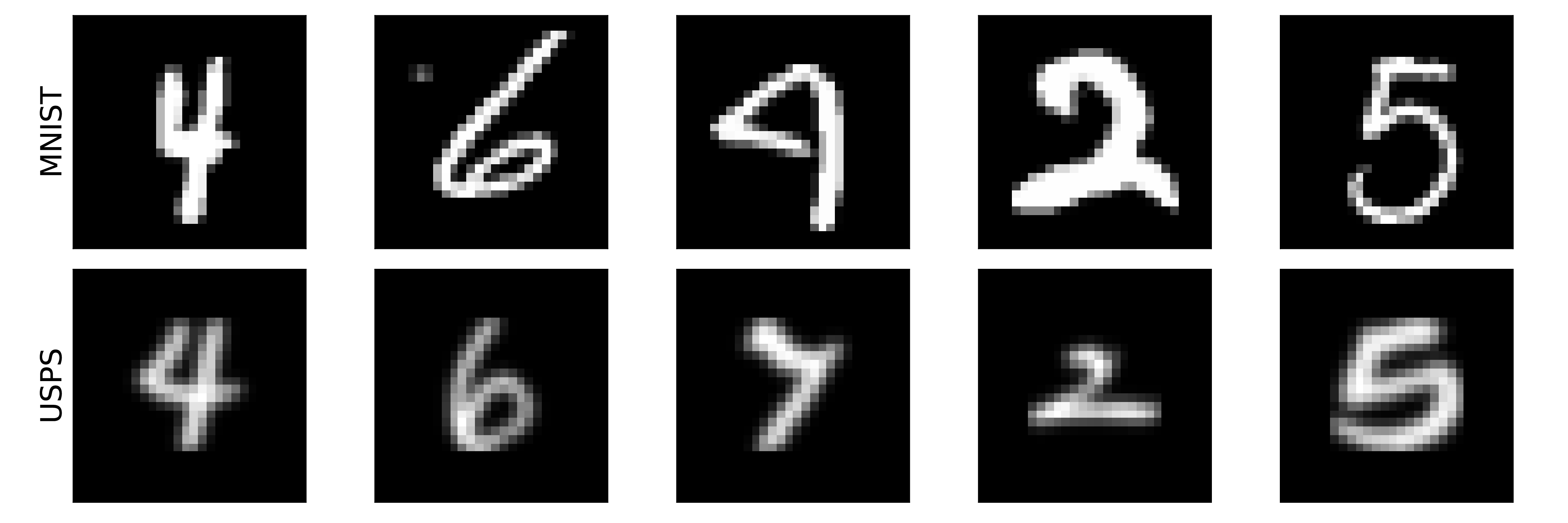
(a) MNIST-USPS Samples

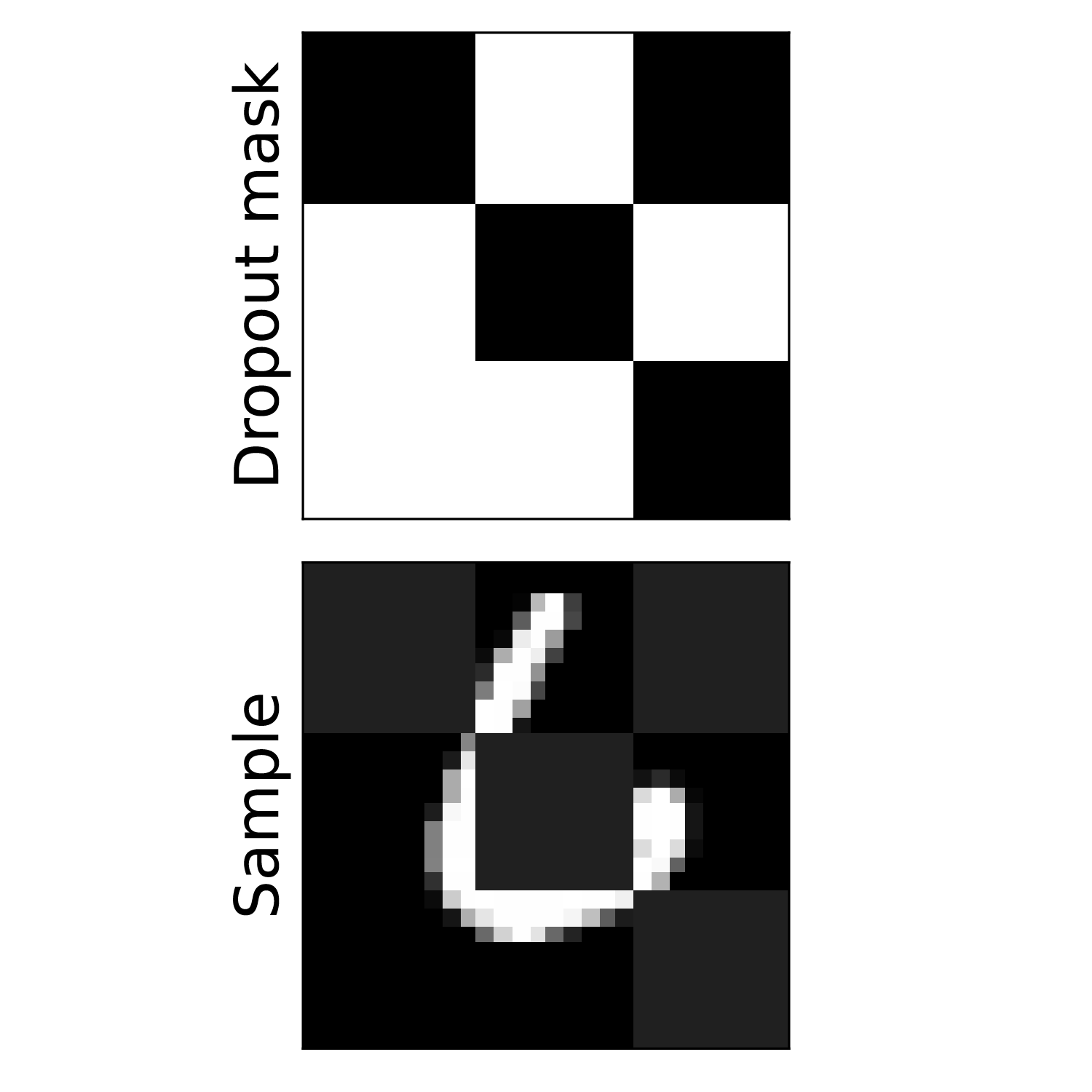
(b) Dropout Mask

Figure S1: Samples used in deep neural network experiments. (a) MNIST samples vs. USPS samples (after zero-padding), used in the Domain Adaptation experiment. (b) Coarse dropout mask applied over all samples in MNIST’s testing set and a sample of the perturbed images, used in the domain shift experiment.

	MNIST-USPS (DA)	MNIST (D)		MNIST (DU)
	Accuracy	Accuracy	L2 error	Accuracy	L2 error
Original	79.3	65.7	0.74	72.6	0.72
OT	76.9	73.4	0.59	61.5	0.71
kOT	79.4	74.0	0.53	60.9	0.73
SA	81.3	64.9	-	72.3	-
FC	84.1	77.6	0.51	67.2	0.59
LOT -L2	86.2	78.2	0.53	77.7	0.56

Table S1: Results for concept drift and domain adaptation for handwritten digits. The classification accuracy and L2-error (transported samples vs. ground truth test samples) are computed for the synthetic drift experiment: Coarse dropout (left) and for the domain adaptation experiment: MNIST to USPS (right). Our method is compared with the accuracy before alignment (Original), entropy-regularized OT, k-means plus OT (kOT), and subspace alignment (SA).

Visualization of transported distributions:

In Figure 5a, we project the distribution of the neural network’s output features (for each set) in 2D using Isomap fit to the MNIST training set’s output features. We use 50 neighbor points in the Isomap algorithm to get a reasonable estimate of the geodesic distance, as we have $10$ well-separated clusters in the output space of the deep neural network in the case of MNIST’s training set. To ensure consistency, we use the projection learned on the MNIST training set with all other sets.

Visualization of transport plans:

We provide further visualization of the transport plans obtained by LOT and FC , for the Domain Adaptation experiment and the unbalanced alignment experiment (Figure S3).

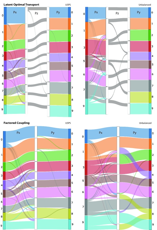
(a)

Figure S3: Visualization of transport plans obtained with LOT and factored coupling. We show the transport plans for LOT (top) and FC (bottom) for the USPS (left) and unbalanced dropout example (right).

Visualization of transported points:

To get a better understanding of how the embedding of each sample is changing after transportation, we provide visualizations of where samples are being transported to in the target space. To describe the target space locally, we find the five nearest neighbors of a sample according to the L2 distance between the transported features of the source sample and the features of the target samples. In Figure S5, we show some of the cases where the three methods, OT , FC and LOT , disagree.

In the top two rows (Figure S5a-b), we see cases where LOT outperforms OT and FC . When all neighbors have the same labels, we can safely assume that we are not in a boundary between classes but deep within a class cluster, so this reflects on the confidence these methods have in their transportation. Both OT and FC confidently map the sample to the wrong region of the space (Figure S5a).

In the bottom two rows (Figure S5c-d), we see more difficult cases. In (Figure S5c), we see that even though the closest neighbor (4 in light green) doesn’t correspond to the ground truth label (7), LOT -L2 seems to be mapping the point to the boundary between classes 7 and 4, and it does in fact classify it correctly. Lastly, in (d), we see that none of the methods is able to recover information lost due to dropout.

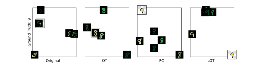
(a)

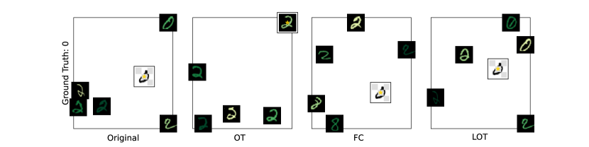
(b)

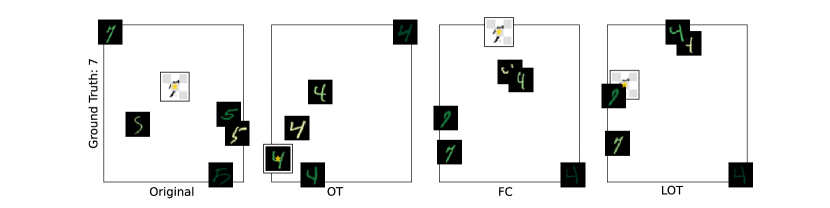
(c)

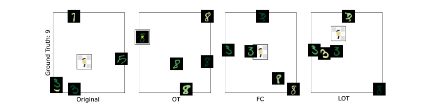
(d)

Figure S5: Neighborhood change after transportation (DU) For the unbalanced transport experiment, we show for multiple perturbed samples (white, marked with a $\star$) the change in the closest neighbors landscape before (Original) and after the transportation, for different methods (OT , FC and LOT ). We find the five nearest neighbors (black) according to the L2 distance between the transported output features of the sample and the features from the target training samples, and arrange the samples in 2D space using the Isomap projection. We apply a gradient filter over the neighbors’ images such that the closest neighbor is light green.

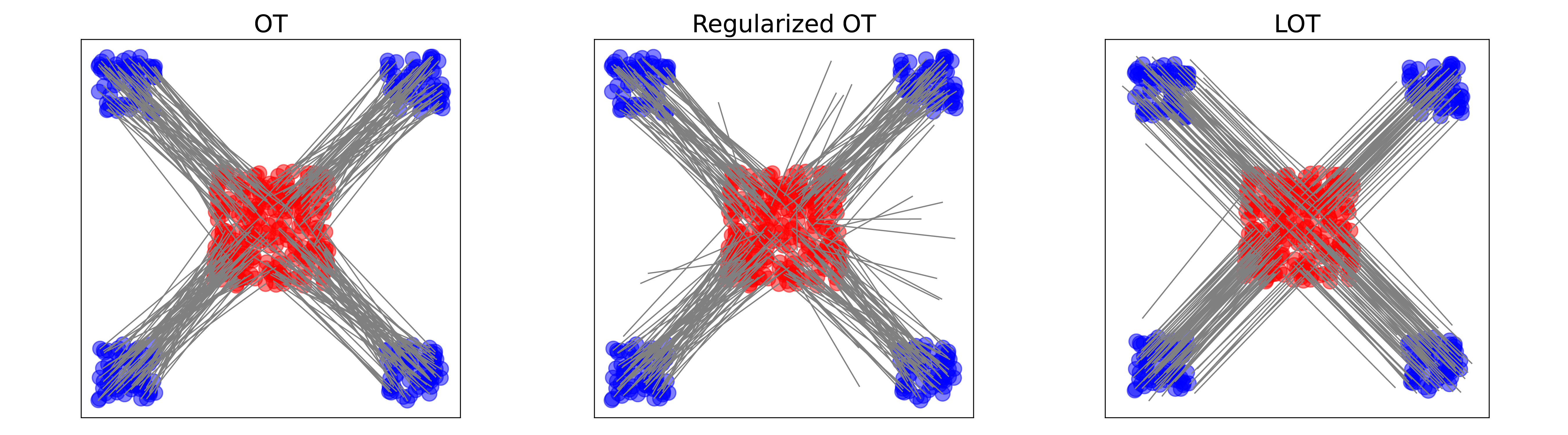
(a)

Figure S6: Fragmented Hypercube. We visualize the estimated transports $\hat{x}=\int yp(y|x)dx$  for OT, regularized OT, and LOT .

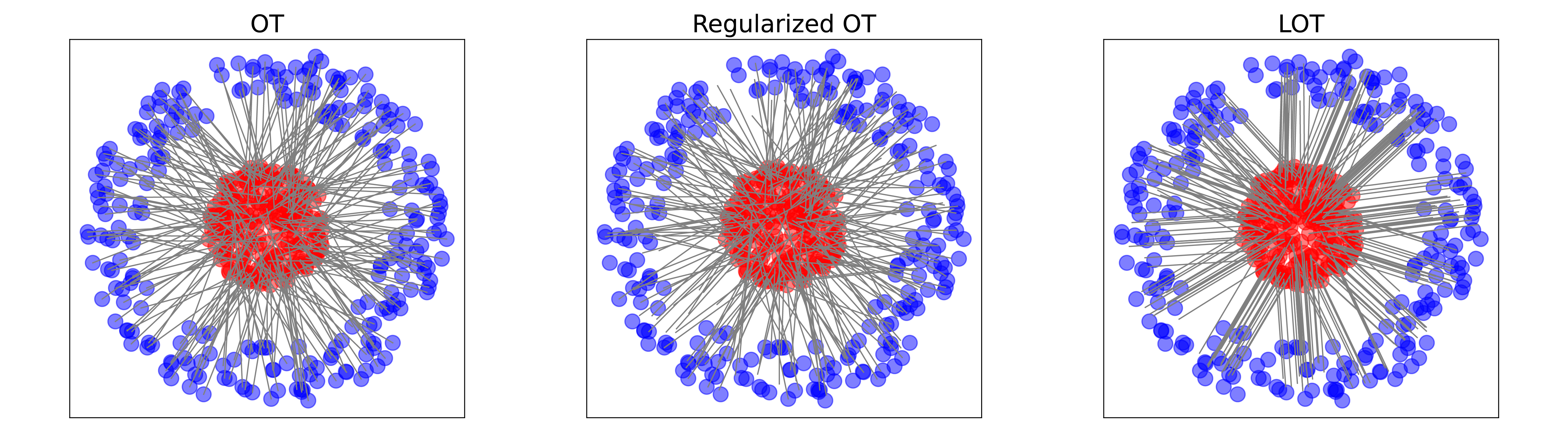
(a)

Figure S7: Disk to Annulus. We visualize the estimated transports $\hat{x}=\int yp(y|x)dx$  for OT, regularized OT, and LOT .

D.2 Additional synthetic experiments

We study the behaviors of LOT for two synthetic experiments performed in (Forrow et al., 2019; Paty & Cuturi, 2019).

Fragmented Hypercube:

In the first experiment, the source distribution is $\mu={\cal{U}}([-1,1]^{d})$ and the target distribution is $\nu=T_{\#}\mu$ (i.e., $\nu\overset{d}{=}T(x),x\overset{d}{=}\mu$), where $T(x)=x+2\text{sign}(x)\odot(e_{1}+e_{2})$, and $e_{i}$ is the canonical basis of $\mathbf{R}^{d}$. In this example, the signal lies only in the first $2$ dimensions while the remaining $d-2$ dimensions are noises. The data shows explicit clustering structure. We investigate the estimated transports $\hat{x}=\int yp(y|x)dx$ produced by OT, entropy- regularized OT, and LOT with $k_{x}=k_{y}=4$ to see if LOT can capture the data structure and whether it provides robust transport. We choose $d=30$ and draw $N=250$ points from each distribution. The result is shown in Figure S6. We see that all methods capture the cluster structure, but both OT and regularized are sensitive to noise in $d-2$ dimensions, while LOT provides a data transport that is more robust against noise in high dimensional space.

Disk to annulus:

In the second experiment, we consider data without separate clustering structure. In this example, the source and target distributions are

$$\mu ={\cal{U}}\{\mathbf{x}\in\mathbb{R}^{d}:0\leq\|(\mathbf{x}_{1},\mathbf{x}_{2})\|_{2}\leq 1,\mathbf{x}_{i}\in\{0,1\},i=3,\dots,d\}$$

$$\nu ={\cal{U}}\{\mathbf{x}\in\mathbb{R}^{d}:2\leq\|(\mathbf{x}_{1},\mathbf{x}_{2})\|_{2}\leq 3,\mathbf{x}_{i}\in\{0,1\},i=3,\dots,d\}.$$

Again only the first $2$ dimensions contain the signal while the rest $d-2$ are noise. We draw $250$ points from each distribution and choose $d=30$. We compare the estimated transports $\hat{x}=\int yp(y|x)dx$ for OT, entropy-regularized OT, and LOT with $k_{x}=k_{y}=15$. In this example, we increase the number of anchors as the annulus can be regarded as having infinite clusters. We visualize the result in Figure S7. We observe that LOT is more regular than the other two, but the support of the target is not fully covered by the transportation. This is because the rank constraint imposed on LOT limits its degree of freedom to transport data.

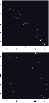
(a) Optimal Transport

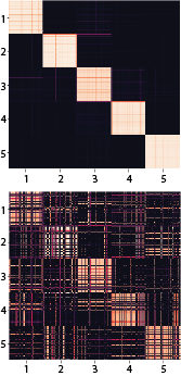
(b) LOT -L2 

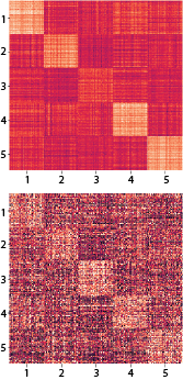
(c) Cross-Correlation

Figure S8: Examining the connection between cluster coherence and transport. In (a-b), we visualize the transport plan obtained by OT and LOT when the different mixture components in the model are weakly correlated (top) and strongly correlated (bottom). In (c), we examine the cross-correlation between points in the source and target for the two conditions.

D.3 Examining the impact of cluster correlation on performance

Next, we study the ability of LOT of capturing clustering structure as the correlation between clusters increases. It is observed in (Lee et al., 2019) that equally spaced clusters (i.e., uniformly distributed subspace angles) are harder to align. In the spirit of measuring cluster similarity as in (Soltanolkotabi et al., 2012), we define the cross-correlation between two clusters ${{\cal{Y}}_{i}}$ and ${{\cal{Y}}_{j}}$ as $\mu_{c}({{\cal{Y}}_{i}},{{\cal{Y}}_{j}}):=\sum_{x\in{{\cal{Y}}_{i}},y\in{{\cal{Y}}_{i}}}\langle x,y\rangle/|{{\cal{Y}}_{i}}||{{\cal{Y}}_{j}}|$. In Fig. S8, we plot the transport plans for GMM with $5$ clusters in two different correlation regimes: (i) the top row shows the regime where the cross-correlation is strong within the same class; (ii) the bottom row shows the uniform correlation case where clusters are approximately equally spaced and the correlations are much more uniform across classes. We observe in both results that LOT has transport plans similar to the cross-correlation in the pattern, while for uniform case, the transport plan of OT seems less structured. This example suggests that LOT can be a useful tool for data visualization.

Appendix E Details of GMM Experiment (E2)

In this experiment, we use a Gaussian mixture model (GMM) with $M$ components in $\mathbb{R}^{d}$ to generate the data for the source and target. For each component, the mean is randomly generated from a random standard normal distribution, and the covariance matrix is generated from a Wishart distribution. To model low-dimensional latent structure, we then apply random $k$-dimensional projection and add a $d$-dimensional standard normal noise to each component. The source and target draw $100$ points from each component independently.

Below we provide the details to each plot of (a) to (e). The default $k$ is set to 5.

Parameters of the data generation:

• (a) We set $M=4,d=30$. We choose a random unit vector and rotate the mean of the component by $\theta$-degree using the vector as the axis.

• (b) $M=4,d=30$. For any ratio $r$ of outliers, we randomly pick up $rn$ number of points and modify its distribution by a linear combination of Gaussian noise and the original point. The variance of Gaussian noise is equal to half the squared mean of the component.

• (c) $M=4$. We increase the dimension $d$. As the signal lies in a $k$-dimensional space, the rest of $d-k$-dimensions are noisy.

• (d) $d=30$. Here we generate a GMM with $10$ components. While the target has $10$ classes with $100$ points per class initially, we vary the number of the source class from $2$ to $10$. The $x$-axis denotes the ratio between the number of components to the source and to the target.

• (e) $d=30,M=4$. We set the number of the source and target anchors to be equal and increase the number from $2$ to $100$. Note that this number also upper bounds the rank of the associated transport plan.

Algorithmic implementation:

• We use the POT: Python Optimal Transport package (Flamary & Courty, 2017) https://pythonot.github.io/ as the implementation for a vanilla optimal transport.

• In all of our GMM experiments, the entropy regularization parameter $\varepsilon$ is set to $10$.

• For the transport estimation, we use the expected transportation defined by a transport plan, which is:

  $$\hat{\mathbf{X}}=\text{diag}(\mu)\mathbf{P}\mathbf{Z}_{2},\text{ for OT\leavevmode\nobreak\ .}$$ (49)

  $$\hat{\mathbf{X}}=\text{diag}(\mu)\mathbf{P}_{x}(\mathbf{Q}_{y}-\mathbf{Q}_{x}),\text{ for {FC}\leavevmode\nobreak\ \cite[citep]{(\@@bibref{AuthorsPhrase1Year}{forrow2019statistical}{\@@citephrase{, }}{})}}$$ (50)

  $$\hat{\mathbf{X}}=\text{diag}(\mu^{-1})\mathbf{P}_{x}\text{diag}((\mathbf{P}_{z}\mathbf{1})^{-1})\mathbf{P}_{z}(\mathbf{Q}_{y}-\mathbf{Q}_{x}),\text{ for {LOT}\leavevmode\nobreak\ (the estimator in Section \ref{sec:algorithm})},$$ (51)

  where $\mathbf{Q}_{x}=\text{diag}(\mu^{-1})\mathbf{P}_{x}^{T}\mathbf{X}^{T}$, $\mathbf{Q}_{y}=\text{diag}(\nu^{-1})\mathbf{P}_{y}\mathbf{Y}$ denote the centroids for FC and LOT .

• We adopt the 1-NN classification rule where the class of a point from the source is predicted by the class of the nearest neighbor (among the target points) of its estimated transportation.

Appendix F Choice of hyperparameters

Code availability:

We provide an implementation of LOT and a demo for a dropout experiment on MNIST in the supplementary file. We use the POT: Python Optimal Transport package (Flamary & Courty, 2017) https://pythonot.github.io/ as the implementation for a vanilla optimal transport.

Hyperparameter tuning:

LOT has two main hyperparameters that must be specified: (i) the number of anchors and (ii) the entropy-regularization parameter epsilon. For domain adaptation experiments (E2-3), the number of anchors was set to $10$, using the prior we had about there being 10 classes of digits. The regularization parameter epsilon was set to $50$; this parameter depends on the scale of the data. We note that in the case of (E2), the standard deviation of the logit outputs of the network was around $10^{3}$. More generally, we proceed as follows when choosing the hyperparameters:

• Number of anchors.  To optimize the number of anchors, one can use domain knowledge or model selection procedures common in clustering. For instance, in the case of MNIST-USPS, we know to expect $10$ clusters, each corresponding to a digit, and set the number of anchors to be at least this amount. In cases where we do not have a priori knowledge about the number of clusters in the data, we can use standard approaches for model selection in clustering (e.g., silhouette score (Rousseeuw, 1987), Calinski-Harabaz index (Caliński & Harabasz, 1974)). In our experiments, we find that the number of anchors can be increased progressively before observing a phase transition (or change point) where the accuracy increases significantly (see Figure 2.e). This change point typically coincides with the number of clusters in the data and can be used to select the number of anchors. Furthermore, while some interpretability may be sacrificed when we overestimate the number of anchors, we find that this does not hinder the performance of the method in terms of the quality of overall transport (see Figure 2.e). This is reminiscent of the elbow phenomena found with clustering methods, so we can imagine utilizing established clustering metrics for tuning these two parameters. This is left for future work, as the simple elbow method was found to be sufficient.

• Entropy- regularization parameter.  The choice of the regularization parameter mainly depends on the scale of the data. In our experiments, we search for the lowest epsilon for which LOT converges using a simple Bisection method. This same approach is used for selecting epsilon for OT in our experiments. We find that the regularization value is inherent to the data and not the task (Exp 2).

References

- Agueh & Carlier (2011) Agueh, M. and Carlier, G. Barycenters in the wasserstein space. SIAM Journal on Mathematical Analysis, 43(2):904–924, 2011.
- Altschuler et al. (2017) Altschuler, J., Niles-Weed, J., and Rigollet, P. Near-linear time approximation algorithms for optimal transport via sinkhorn iteration. In Advances in neural information processing systems, pp. 1964–1974, 2017.
- Altschuler et al. (2019) Altschuler, J., Bach, F., Rudi, A., and Niles-Weed, J. Massively scalable sinkhorn distances via the nyström method. In Advances in Neural Information Processing Systems, pp. 4427–4437, 2019.
- Alvarez-Melis & Fusi (2020) Alvarez-Melis, D. and Fusi, N. Geometric dataset distances via optimal transport. arXiv preprint arXiv:2002.02923, 2020.
- Alvarez-Melis et al. (2018) Alvarez-Melis, D., Jaakkola, T., and Jegelka, S. Structured optimal transport. In Proceedings of the Twenty-First International Conference on Artificial Intelligence and Statistics, pp. 1771–1780, 2018.
- Alvarez-Melis et al. (2019) Alvarez-Melis, D., Jegelka, S., and Jaakkola, T. S. Towards optimal transport with global invariances. In Proceedings of the Twenty-Second International Conference on Artificial Intelligence and Statistics, pp. 1870–1879. PMLR, 2019.
- Arthur & Vassilvitskii (2006) Arthur, D. and Vassilvitskii, S. k-means++: The advantages of careful seeding. Technical report, Stanford, 2006.
- Benamou et al. (2015) Benamou, J.-D., Carlier, G., Cuturi, M., Nenna, L., and Peyré, G. Iterative bregman projections for regularized transportation problems. SIAM Journal on Scientific Computing, 37(2):A1111–A1138, 2015.
- Bonneel et al. (2016) Bonneel, N., Peyré, G., and Cuturi, M. Wasserstein barycentric coordinates: histogram regression using optimal transport. ACM Trans. Graph., 35(4):71–1, 2016.
- Caliński & Harabasz (1974) Caliński, T. and Harabasz, J. A dendrite method for cluster analysis. Communications in Statistics, 3(1):1–27, 1974. doi: 10.1080/03610927408827101. URL https://www.tandfonline.com/doi/abs/10.1080/03610927408827101.
- Chen et al. (2018) Chen, Y., Georgiou, T. T., and Tannenbaum, A. Optimal transport for gaussian mixture models. IEEE Access, 7:6269–6278, 2018.
- Courty et al. (2014) Courty, N., Flamary, R., and Tuia, D. Domain adaptation with regularized optimal transport. In Machine Learning and Knowledge Discovery in Databases, pp. 274–289. Springer, 2014.
- Courty et al. (2017) Courty, N., Flamary, R., Tuia, D., and Rakotomamonjy, A. Optimal transport for domain adaptation. IEEE Transactions on Pattern Analysis and Machine Intelligence, 39(9):1853–1865, 2017.
- Cuturi (2013) Cuturi, M. Sinkhorn distances: Lightspeed computation of optimal transport. In Advances in Neural Information Processing Systems, pp. 2292–2300, 2013.
- Cuturi & Avis (2014) Cuturi, M. and Avis, D. Ground metric learning. J. Mach. Learn. Res., 15(1):533–564, 2014.
- Cuturi & Doucet (2014) Cuturi, M. and Doucet, A. Fast computation of wasserstein barycenters. pp. 685–693, 2014.
- Cuturi & Peyré (2016) Cuturi, M. and Peyré, G. A smoothed dual approach for variational wasserstein problems. SIAM Journal on Imaging Sciences, 9(1):320–343, 2016.
- Dessein et al. (2017) Dessein, A., Papadakis, N., and Deledalle, C.-A. Parameter estimation in finite mixture models by regularized optimal transport: A unified framework for hard and soft clustering. arXiv preprint arXiv:1711.04366, 2017.
- Dhouib et al. (2020) Dhouib, S., Redko, I., Kerdoncuff, T., Emonet, R., and Sebban, M. A swiss army knife for minimax optimal transport. In Proceedings of the 37th International Conference on Machine Learning, 2020.
- Doersch et al. (2015) Doersch, C., Gupta, A., and Efros, A. A. Unsupervised visual representation learning by context prediction. In IEEE International Conference on Computer Vision, pp. 1422–1430, 2015.
- Dykstra (1983) Dykstra, R. L. An algorithm for restricted least squares regression. Journal of the American Statistical Association, 78(384):837–842, 1983.
- Fernando et al. (2013) Fernando, B., Habrard, A., Sebban, M., and Tuytelaars, T. Unsupervised visual domain adaptation using subspace alignment. In IEEE International Conference on Computer Vision, pp. 2960–2967, 2013.
- Flamary & Courty (2017) Flamary, R. and Courty, N. POT Python optimal transport library, 2017. URL https://pythonot.github.io/.
- Forrow et al. (2019) Forrow, A., Hütter, J.-C., Nitzan, M., Rigollet, P., Schiebinger, G., and Weed, J. Statistical optimal transport via factored couplings. In Proceedings of the Twenty-Second International Conference on Artificial Intelligence and Statistics, pp. 2454–2465, 2019.
- Genevay et al. (2019) Genevay, A., Dulac-Arnold, G., and Vert, J.-P. Differentiable deep clustering with cluster size constraints. arXiv preprint arXiv:1910.09036, 2019.
- Graf & Luschgy (2007) Graf, S. and Luschgy, H. Foundations of quantization for probability distributions. Springer, 2007.
- Gramfort et al. (2015) Gramfort, A., Peyré, G., and Cuturi, M. Fast optimal transport averaging of neuroimaging data. In Information Processing in Medical Imaging, pp. 261–272. Springer, 2015.
- He et al. (2020) He, K., Fan, H., Wu, Y., Xie, S., and Girshick, R. Momentum contrast for unsupervised visual representation learning. In Proceedings of the IEEE/CVF Conference on Computer Vision and Pattern Recognition, pp. 9729–9738, 2020.
- Ho et al. (2017) Ho, N., Nguyen, X., Yurochkin, M., Bui, H. H., Huynh, V., and Phung, D. Multilevel clustering via wasserstein means. arXiv preprint arXiv:1706.03883, 2017.
- Kusner et al. (2015) Kusner, M., Sun, Y., Kolkin, N., and Weinberger, K. From word embeddings to document distances. In Proceedings of the Thirty-Forth International Conference on Artificial Intelligence and Statistics, pp. 957–966, 2015.
- Laclau et al. (2017) Laclau, C., Redko, I., Matei, B., Bennani, Y., and Brault, V. Co-clustering through optimal transport. arXiv preprint arXiv:1705.06189, 2017.
- Lee et al. (2019) Lee, J., Dabagia, M., Dyer, E., and Rozell, C. Hierarchical optimal transport for multimodal distribution alignment. In Advances in Neural Information Processing Systems, pp. 13474–13484, 2019.
- Li & Wang (2008) Li, J. and Wang, J. Z. Real-time computerized annotation of pictures. IEEE transactions on pattern analysis and machine intelligence, 30(6):985–1002, 2008.
- Liero et al. (2018) Liero, M., Mielke, A., and Savaré, G. Optimal entropy-transport problems and a new hellinger–kantorovich distance between positive measures. Inventiones mathematicae, 211(3):969–1117, 2018.
- Manay et al. (2006) Manay, S., Cremers, D., Hong, B.-W., Yezzi, A. J., and Soatto, S. Integral invariants for shape matching. IEEE Transactions on pattern analysis and machine intelligence, 28(10):1602–1618, 2006.
- Martin Arjovsky & Bottou (2017) Martin Arjovsky, S. and Bottou, L. Wasserstein generative adversarial networks. In Proceedings of the 34th International Conference on Machine Learning, 2017.
- Paty & Cuturi (2019) Paty, F.-P. and Cuturi, M. Subspace robust wasserstein distances. 2019.
- Pele & Werman (2009) Pele, O. and Werman, M. Fast and robust earth mover’s distances. In 2009 IEEE 12th International Conference on Computer Vision, pp. 460–467. IEEE, 2009.
- Peyré et al. (2019) Peyré, G., Cuturi, M., et al. Computational optimal transport: With applications to data science. Foundations and Trends® in Machine Learning, 11(5-6):355–607, 2019.
- Rousseeuw (1987) Rousseeuw, P. J. Silhouettes: A graphical aid to the interpretation and validation of cluster analysis. Journal of Computational and Applied Mathematics, 20:53 – 65, 1987. ISSN 0377-0427. doi: https://doi.org/10.1016/0377-0427(87)90125-7. URL http://www.sciencedirect.com/science/article/pii/0377042787901257.
- Santambrogio (2015) Santambrogio, F. Optimal transport for applied mathematicians. Birkäuser, NY, 55(58-63):94, 2015.
- Sato et al. (2020) Sato, R., Cuturi, M., Yamada, M., and Kashima, H. Fast and robust comparison of probability measures in heterogeneous spaces. arXiv preprint arXiv:2002.01615, 2020.
- Solomon et al. (2014) Solomon, J., Rustamov, R., Guibas, L., and Butscher, A. Earth mover’s distances on discrete surfaces. ACM Trans. Graph., 33(4):1–12, 2014.
- Solomon et al. (2015) Solomon, J., De Goes, F., Peyré, G., Cuturi, M., Butscher, A., Nguyen, A., Du, T., and Guibas, L. Convolutional wasserstein distances: Efficient optimal transportation on geometric domains. ACM Trans. Graph., 34(4):1–11, 2015.
- Soltanolkotabi et al. (2012) Soltanolkotabi, M., Candes, E. J., et al. A geometric analysis of subspace clustering with outliers. The Annals of Statistics, 40(4):2195–2238, 2012.
- Tolstikhin et al. (2017) Tolstikhin, I., Bousquet, O., Gelly, S., and Schoelkopf, B. Wasserstein auto-encoders. arXiv preprint arXiv:1711.01558, 2017.
- Villani (2008) Villani, C. Optimal transport: old and new, volume 338. Springer Science & Business Media, 2008.
- Weed et al. (2019) Weed, J., Bach, F., et al. Sharp asymptotic and finite-sample rates of convergence of empirical measures in wasserstein distance. Bernoulli, 25(4A):2620–2648, 2019.
- Xu et al. (2020) Xu, H., Luo, D., Henao, R., Shah, S., and Carin, L. Learning autoencoders with relational regularization. 2020.
- Ye et al. (2017) Ye, J., Wu, P., Wang, J. Z., and Li, J. Fast discrete distribution clustering using wasserstein barycenter with sparse support. IEEE Transactions on Signal Processing, 65(9):2317–2332, 2017.
- Yurochkin et al. (2019) Yurochkin, M., Claici, S., Chien, E., Mirzazadeh, F., and Solomon, J. M. Hierarchical optimal transport for document representation. In Advances in Neural Information Processing Systems, pp. 1601–1611, 2019.