OBoW: Online Bag-of-Visual-Words Generation for Self-Supervised Learning

Abstract

Learning image representations without human supervision is an important and active research field. Several recent approaches have successfully leveraged the idea of making such a representation invariant under different types of perturbations, especially via contrastive-based instance discrimination training. Although effective visual representations should indeed exhibit such invariances, there are other important characteristics, such as encoding contextual reasoning skills, for which alternative reconstruction-based approaches might be better suited.

With this in mind, we propose a teacher-student scheme to learn representations by training a convolutional net to reconstruct a bag-of-visual-words (BoW) representation of an image, given as input a perturbed version of that same image. Our strategy performs an online training of both the teacher network (whose role is to generate the BoW targets) and the student network (whose role is to learn representations), along with an online update of the visual-words vocabulary (used for the BoW targets). This idea effectively enables fully online BoW-guided unsupervised learning. Extensive experiments demonstrate the interest of our BoW-based strategy, which surpasses previous state-of-the-art methods (including contrastive-based ones) in several applications. For instance, in downstream tasks such Pascal object detection, Pascal classification and Places205 classification, our method improves over all prior unsupervised approaches, thus establishing new state-of-the-art results that are also significantly better even than those of supervised pre-training. We provide the implementation code at https://github.com/valeoai/obow.

1 Introduction

Learning unsupervised image representations based on convolutional neural nets (convnets) has attracted a significant amount of attention recently. Many different types of convnet-based methods have been proposed in this regard, including methods that rely on using annotation-free pretext tasks [16, 28, 46, 53, 57, 85], generative methods that model the image data distribution [17, 18, 21], as well as clustering-based approaches [4, 6, 7].

Several recent methods opt to learn representations via instance-discrimination training [9, 20, 35, 80], typically implemented in a contrastive learning framework [12, 34]. The primary focus here is to learn low-dimensional image / instance embeddings that are invariant to intra-image variations while being discriminative among different images. Although these methods manage to achieve impressive results, they focus less on other important aspects in representation learning, such as contextual reasoning, for which alternative reconstruction-based approaches [15, 57, 85, 86] might be better suited. For instance, the task of predicting from an image region the contents of the entire image requires to recognize the visual concepts depicted in the provided region and then to infer from them the structure of the entire scene. So, training for such a task has the potential of squeezing out more information from the training images and of learning richer and more powerful representations.

However, reconstructing image pixels is an ambiguous and hard-to-optimize task that forces the convnet to spend a lot of capacity on modeling low-level pixel details. It is all the more unnecessary when the final goal deals with high-level image understanding, such as image classification. To leverage the advantages of the reconstruction principle without focusing on unimportant pixel details, one can focus on reconstruction over high-level visual concepts, referred to as visual words. For instance, BoWNet [26] derived a teacher-student learning scheme following this principle. In this teacher-student setting, given an image, the teacher extracts feature maps that are then quantized in a spatially-dense way over a vocabulary of visual words. Then, the resulting visual words-based image description is exploited for training the student on the self-supervised task of reconstructing the distribution of the visual words of an image, i.e., its bag-of-words (BoW) representation [81], given as input a perturbed version of that same image. By solving this reconstruction task the student is forced to learn perturbation-invariant and context-aware representations while “ignoring” pixel details.

Despite its advantages, the BoWNet approach exhibits some important limitations that do not allow it to fully exploit the potential of the BoW-based reconstruction task. One of them is that it relies on the availability of an already pre-trained teacher network. More importantly, it assumes that this teacher remains static throughout training. However, due to the fact that during the training process the quality of the student’s representations will surpass the teacher’s ones, a static teacher is prone to offer a suboptimal supervisory signal to the student and to lead to an inefficient usage of the computational budget for training.

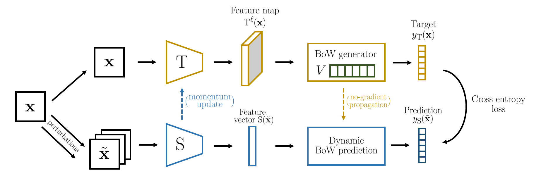
Figure 1: Unsupervised learning with Bag-of-Words guidance. Two encoders $\mathrm{T}$ and $\mathrm{S}$ learn at different tempos by interacting and learning from each other. An image $\mathbf{x}$ is passed through the encoder $\mathrm{T}$ and its output feature maps $\mathrm{T}^{\ell}(\mathbf{x})$ are embedded into a BoW representation $y_{\mathrm{T}}(\mathbf{x})$ over a vocabulary $V$ of features from $\mathrm{T}$. The vocabulary $V$ is updated at each step. The encoder $\mathrm{S}$ aims to reconstruct $y_{\mathrm{T}}(\mathbf{x})$ from data-augmented instances $\tilde{\mathbf{x}}$. A dynamic BoW-prediction head learns to leverage the continuously updated vocabulary $V$ to compute the BoW representation from the features $\mathrm{S}(\tilde{\mathbf{x}})$. $\mathrm{T}$ follows slowly the learning trajectory of $\mathrm{S}$ via momentum updates.

In this paper, we propose a BoW-based self-supervised approach that overcomes the aforementioned limitations. To that end, our main technical contributions are three-fold:

1. We design a novel fully online teacher-student learning scheme for BoW-based self-supervised training (Fig. 1). This is achieved by online training of the teacher and the student networks.

2. We significantly revisit key elements of the BoW-guided reconstruction task. This includes the proposal of a dynamic BoW prediction module used for reconstructing the BoW representation of the student image. This module is carefully combined with adequate online updates of the visual-words vocabulary used for the BoW targets.

3. We enforce the learning of powerful contextual reasoning skills in our image representations. Revisiting data augmentation with aggressive cropping and spatial image perturbations, and exploiting multi-scale BoW reconstruction targets, we equip our student network with a powerful feature representation.

Overall, the proposed method leads to a simpler and much more efficient training methodology for the BoW-guided reconstruction task that manages to learn significantly better image representations and therefore achieves or even surpasses the state of the art in several unsupervised learning benchmarks. We call our method OBoW after the online BoW generation mechanism that it uses.

2 Related Work

Bags of visual words.   Bag-of-visual-words representations are powerful image models able to encode image statistics from hundreds of local features. Thanks to that, they were used extensively in the past [13, 42, 58, 66, 71] and continue to be a key ingredient of several recent deep learning approaches [2, 26, 29, 40]. Among them, BoWNet [26] was the first work to use BoWs as reconstruction targets for unsupervised representation learning. Inspired by it, we propose a novel BoW-based self-supervised method with a more simple and effective training methodology that includes generating BoW targets in a fully online manner and further enforcing the learning of context-aware representations.

Self-supervised learning.   A prominent paradigm for unsupervised representation learning is to train a convnet on an artificially designed annotation-free pretext task, e.g., [3, 10, 16, 28, 47, 52, 53, 76, 78, 84, 88]. Many works rely on pretext reconstruction tasks [1, 30, 46, 57, 59, 74, 85, 86, 88], where the reconstruction target is defined at image pixel level. This is in stark contrast with our method, which uses a reconstruction task defined over high-level visual concepts (i.e., visual words) that are learnt with a teacher-student scheme in a fully online manner.

Instance discrimination and contrastive objectives.   Recently, unsupervised methods based on contrastive learning objectives [8, 9, 23, 24, 35, 38, 41, 51, 54, 69, 77, 80] have shown great results. Among them, contrastive-based instance discrimination training [9, 19, 35, 43, 80] is the most prominent example. In this case, a convnet is trained to learn image representations that are invariant to several perturbations and at the same time discriminative among different images (instances). Our method also learns intra-image invariant representations, since the convnet must predict the same BoW target (computed from the original image) regardless of the applied perturbation. More than that however, our work also places emphasis on learning context-aware representations, which, we believe, is another important characteristic that effective representations should have. In that respect, it is closer to contrastive-based approaches that target to learn context-aware representations by predicting (in a contrastive way) the state of missing image patches [38, 54, 72].

Teacher-student approaches.   This paradigm has a long research history [25, 65] and it is frequently used for distilling a single large network or an ensemble, the teacher, into a smaller network, the student [5, 39, 44, 56]. This setting has been revisited in the context of semi-supervised learning where the teacher is no longer fixed but evolves during training [45, 68, 73]. In self-supervised learning, BowNet [26] trains a student to match the BoW representations produced by a self-supervised pre-trained teacher. MoCo [35] relies on a slow-moving momentum-updated teacher to generate up-to-date representations to fill a memory bank of negative images. BYOL [33], which is a method concurrent to our work, also uses a momentum-updated teacher and trains the student to predict features generated by the teacher. However, BYOL, similar to contrastive-based instance discrimination methods, uses low-dimensional global image embeddings as targets (produced from the final convnet output) and primarily focuses on making them intra-image invariant. On the contrary, our training targets are produced by converting the intermediate teacher feature maps to high-dimensional BoW vectors that capture multiple local visual concepts, thus constituting a richer target representation. Moreover, they are built over an online-updated vocabulary from randomly sampled local features, expressing the current image as statistics over this vocabulary (see § 3.1). Therefore, our BoW targets expose fewer learning “shortcuts” (a critical aspect in self-supervised learning [3, 16, 53, 78]), thus preventing to a larger extent teacher-student collapse and overfitting.

Relation to SwAV [8].   OBoW presents some similarity (e.g., using online vocabularies) with SwAV [8]. However, the prediction tasks fundamentally differ: OBoW exploits a BoW prediction task while SwAV uses an image-cluster prediction task  [4, 6, 7]. BoW targets are much richer representations than image-cluster assignments: a BoW encodes all the local-feature statistics of an image whereas an image-cluster assignment encodes only one global image feature.

3 Our approach

Here we explain our proposed approach for learning image representations by reconstructing bags of visual words. We start with an overview of our method.

Overview.   The bag-of-words reconstruction task involves a student convnet $\mathrm{S}(\cdot)$ that learns image representations, and a teacher convnet $\mathrm{T}(\cdot)$ that generates BoW targets used for training the student network. The student $\mathrm{S}(\cdot)$ is parameterized by $\theta_{\mathrm{S}}$ and the teacher $\mathrm{T}(\cdot)$ by $\theta_{\mathrm{T}}$.

To generate a BoW representation $y_{\mathrm{T}}(\mathbf{x})$ out of an image $\mathbf{x}$, the teacher first extracts the feature map $\mathrm{T}^{\ell}(\mathbf{x})\in\mathbb{R}^{c_{\ell}\times h_{\ell}\times w_{\ell}}$, of spatial size $h_{\ell}\times w_{\ell}$ with $c_{\ell}$ channels, from its $\ell^{\rm th}$ layer (in our experiments $\ell$ is either the last $L$ or penultimate $L\!-\!1$ convolutional layer of $\mathrm{T}(\cdot)$). It quantizes the $c_{\ell}$-dimensional feature vectors $\mathrm{T}^{\ell}(\mathbf{x})[u]$ at each location $u\in\{1,\cdots,h_{\ell}\times w_{\ell}\}$ of the feature map over a vocabulary $V=[\mathbf{v}_{1},\ldots,\mathbf{v}_{K}]$ of $K$ visual words of dimension $c_{\ell}$. This quantization process produces for each location $u$ a $K$-dimensional code vector $q(\mathbf{x})[u]$ that encodes the assignment of $\mathrm{T}(\mathbf{x})[u]$ to its closest (in terms of squared Euclidean distance) visual word(s). Then, the teacher reduces the quantized feature maps $q(\mathbf{x})$ to a $K$-dimensional BoW, $\tilde{y}_{\mathrm{T}}(\mathbf{x})$, by channel-wise max-pooling, i.e., $\tilde{y}_{\mathrm{T}}(\mathbf{x})[k]=\max_{u}q(\mathbf{x})[u][k]$ (alternatively, the reduction can be performed with average pooling), where $q(\mathbf{x})[u][k]$ is the assignment value of the code $q(\mathbf{x})[u]$ for the $k^{\mathrm{th}}$ word. Finally, $\tilde{y}_{\mathrm{T}}(\mathbf{x})$ is converted into a probability distribution over the visual words by $L_{1}$-normalization, i.e., $y_{\mathrm{T}}(\mathbf{x})[k]=\frac{\tilde{y}_{\mathrm{T}}(\mathbf{x})[k]}{\sum_{k^{\prime}}\tilde{y}_{\mathrm{T}}(\mathbf{x})[k^{\prime}]}$.

To learn image representations, the student gets as input a perturbed version of the image $\mathbf{x}$, denoted as $\tilde{\mathbf{x}}$, and is trained to reconstruct the BoW representation $y_{\mathrm{T}}(\mathbf{x})$, produced by the teacher, of the original unperturbed image $\mathbf{x}$. To that end, it first extracts a global vector representation $\mathrm{S}(\tilde{\mathbf{x}})\in\mathbb{R}^{c}$ (with $c$ channels) from the entire image $\tilde{\mathbf{x}}$ and then applies a linear-plus-softmax layer to $\mathrm{S}(\tilde{\mathbf{x}})$, as follows:

$$y_{\mathrm{S}}(\tilde{\mathbf{x}})[k]=\frac{\exp(\mathbf{w}_{k}^{\top}\mathrm{S}(\tilde{\mathbf{x}}))}{\sum_{k^{\prime}}\exp(\mathbf{w}_{k^{\prime}}^{\top}\mathrm{S}(\tilde{\mathbf{x}}))},$$ (1)

where $W=[\mathbf{w}_{1},\cdots,\mathbf{w}_{K}]$ are the $c$-dimensional weight vectors (one per word) of the linear layer. The $K$-dimensional vector $y_{\mathrm{S}}(\tilde{\mathbf{x}})$ is the predicted softmax probability of the target $y_{\mathrm{T}}(\mathbf{x})$. Hence, the training loss that is minimized for a single image $\mathbf{x}$ is the cross-entropy loss

$$\mathrm{CE}\big{(}y_{\mathrm{S}}(\tilde{\mathbf{x}}),y_{\mathrm{T}}(\mathbf{x})\big{)}=-\sum_{k=1}^{K}y_{\mathrm{T}}(\mathbf{x})[k]\log\big{(}y_{\mathrm{S}}(\tilde{\mathbf{x}})[k]\big{)}$$ (2)

between the softmax distribution $y_{\mathrm{S}}(\tilde{\mathbf{x}})$ predicted by the student from the perturbed image $\tilde{\mathbf{x}}$, and the BoW distribution $y_{\mathrm{T}}(\mathbf{x})$ of the unperturbed image $\mathbf{x}$ given by the teacher.

Our technical contributions.   In the following, we explain (i) in § 3.1, how to construct a fully online training methodology for the teacher, the student and the visual-words vocabulary, (ii) in § 3.2, how to implement a dynamic approach for the BoW prediction that can adapt to continuously-changing vocabularies of visual words, and finally (iii) in § 3.3, how to significantly enhance the learning of contextual reasoning skills by utilizing multi-scale BoW reconstruction targets and by revisiting the image augmentation schemes.

3.1 Fully online BoW-based learning

To make the BoW targets encode more high-level features, BoWNet pre-trains the teacher convnet $\mathrm{T}(\cdot)$ with another unsupervised method, such as RotNet [28], and computes the vocabulary $V$ for quantizing the teacher feature maps off-line by applying k-means on a set of teacher feature maps extracted from training images. After the end of the student training, during which the teacher’s parameters remain frozen, the student becomes the new teacher $\mathrm{T}(\cdot)\leftarrow\mathrm{S}(\cdot)$, a new vocabulary $V$ is learned off-line from the new teacher, and a new student is trained, starting a new training cycle. In this case however, (a) the final success depends on the quality of the first pre-trained teacher, (b) the teacher and the BoW reconstruction targets $y_{\mathrm{T}}(\mathbf{x})$ remain frozen for long periods of time, which, as already explained, results in a suboptimal training signal, and (c) multiple training cycles are required, making the overall training time consuming.

To address these important limitations, in this work we propose a fully online training methodology that allows the teacher to be continuously updated as the student training progresses, with no need for off-line k-means stages. This requires an online updating scheme for the teacher as well as for the vocabulary of visual words used for generating the BoW targets, both of which are detailed below.

Updating the teacher network.   Inspired by MoCo [35], the parameters $\theta_{\mathrm{T}}$ of the teacher convnet are an exponential moving average of the student parameters. Specifically, at each training iteration the parameters $\theta_{\mathrm{T}}$ are updated as

$$\theta_{\mathrm{T}}\leftarrow\alpha\cdot\theta_{\mathrm{T}}+(1-\alpha)\cdot\theta_{\mathrm{S}},$$ (3)

where $\alpha\in[0,1]$ is a momentum coefficient. Note that, as a consequence, the teacher has to share exactly the same architecture as the student. With a proper tuning of $\alpha$, e.g., $\alpha=0.99$, this update rule allows slow and continuous updates of the teacher, avoiding rapid changes of its parameters, such as with $\alpha=0$, which would make the training unstable. As in MoCo, for its batch-norm units, the teacher maintains different batch-norm statistics from the student.

Updating the visual-words vocabulary.   Since the teacher is continuously updated, off-line learning of $V$ is not a viable option. Instead, we explore two solutions for computing $V,$ online k-means and a queue-based vocabulary.

Online k-means. One possible choice for updating the vocabulary is to apply online k-means clustering after each training step. Specifically, as proposed in VQ-VAE [55, 62], we use exponential moving average for vocabulary updates. A critical issue that arises in this case is that, as training progresses, the features distribution changes over time. The visual words computed by online k-means do not adapt to this distribution shift leading to extremely unbalanced cluster assignments and even to assignments that collapse to a single cluster. In order to counter this effect, we investigate different strategies: (a) detection of rarely used visual words over several mini-batches and replacement of these words with a randomly sampled feature vector from the current mini-batch; (b) enforcing uniform assignments to each cluster thanks to the Sinkhorn optimization as in, e.g., [4, 8]. For more details see §D.

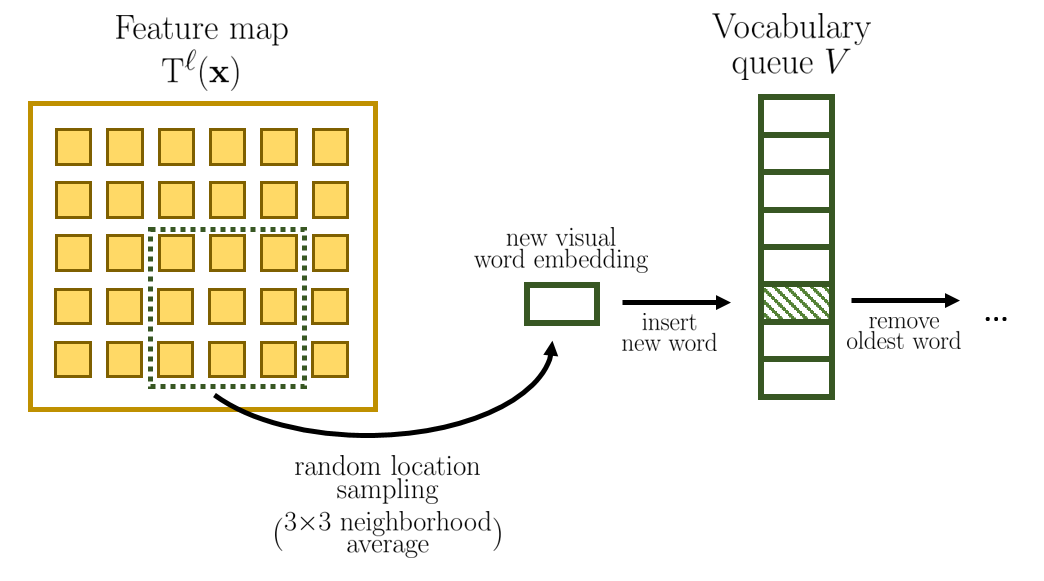
Figure 2: Vocabulary queue from randomly sampled local features. For each input image $\mathbf{x}$ to $\mathrm{T}$, “local” features are pooled from $\mathrm{T}^{\ell}(\mathbf{x})$ by averaging over $3\times 3$ sliding windows. One of the resulting vectors is selected randomly and added as visual word to the vocabulary queue, replacing the oldest word in the vocabulary.

A queue-based vocabulary. In this case, the vocabulary $V$ of visual words is a $K$-sized queue of random features. At each step, after computing the assignment codes over the current vocabulary $V,$ we update $V$ by selecting one feature vector per image from the current mini-batch, inserting it to the queue, and removing the oldest item in the queue if its size exceeds $K$. Hence, the visual words in $V$ are always feature vectors from past mini-batches. We explore three different ways to select these local feature vectors: (a) uniform random sampling of one feature vector in $\mathrm{T}^{\ell}(\mathbf{x})$; (b) global average pooling of $\mathrm{T}^{\ell}(\mathbf{x})$ (average feature vector of each image); (c) an intermediate approach between (a) and (b) which consists of a local average pooling with a $3\times 3$ kernel (stride $1$, padding $0$) of the feature map $\mathrm{T}^{\ell}(\mathbf{x})$ followed by a uniform random sampling of one of the resulting feature vectors (Fig. 2). Our intuition for option (c) is that, assuming that the local features in a $3\times 3$ neighborhood belong to one common visual concept, then local averaging selects a more representative visual-word feature from this neighborhood than simply sampling at random one local feature (option (a)). Likewise, the global averaging option (b) produces a representative feature from an entire image, which however, might result in overly coarse visual word features.

The advantage of the queue-based solution over online k-means is that it is simpler to implement and it does not require any extra mechanism for avoiding unbalanced clusters, since at each step the queue is updated with new randomly sampled features. Indeed, in our experiments, the queue-based vocabulary with option (c) provided the best results.

Generating BoW targets with soft-assignment codes.   For generating the BoW targets, we use soft-assignments instead of the hard-assignments used in BoWNet. This is preferable from an optimization perspective due to the fact that the vocabulary of visual words is continuously evolving. We thus compute the assignment codes $q(\mathbf{x})[u]$ as

$$q(\mathbf{x})[u][k]=\frac{\exp(-\frac{1}{\delta}\,\|\mathrm{T}^{\ell}(\mathbf{x})[u]-\mathbf{v}_{k}\|^{2}_{2})}{\sum_{k^{\prime}}\exp(-\frac{1}{\delta}\,\|\mathrm{T}^{\ell}(\mathbf{x})[u]-\mathbf{v}_{k^{\prime}}\|^{2}_{2})}.$$ (4)

The parameter $\delta$ is a temperature value that controls the softness of the assignment. We use $\delta=\delta_{\rm base}\cdot\bar{\mu}_{\text{MSD}}$, where $\delta_{\rm base}>0$ and $\bar{\mu}_{\text{MSD}}$ is the exponential moving average (with momentum $0.99$) of the mean squared distance of the feature vectors in $\mathrm{T}^{\ell}(\mathbf{x})$ from their closest visual words. The reason for using an adaptive temperature instead of a constant one is due to the change of magnitude of the feature activations during training, which induces a change of scale of the distances between the feature vectors and the words.

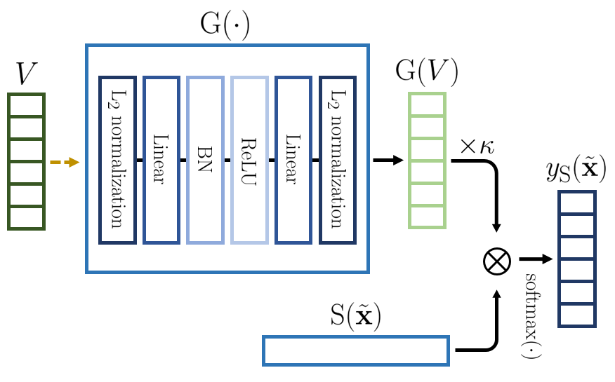
Figure 3: Dynamic BoW-prediction head. $\mathrm{G}(\cdot)$ learns to quickly adapt to the visual words in the continuously refreshed vocabulary $V$. The outputs $\mathrm{G}(V)$ are in fact weights that are used for mapping the features $\mathrm{S}(\tilde{\mathbf{x}})$ to the corresponding BoW vector $y_{\mathrm{S}}(\tilde{\mathbf{x}})$.

3.2 Dynamic bag-of-visual-word prediction

To learn effective image representations, the student must predict the BoW distribution over $V$ of an image using as input a perturbed version of that same image. However, in our method the vocabulary is constantly updated and the visual words are changing or being replaced from one step to the next. Therefore, predicting the BoW distribution over a continuously updating vocabulary $V$ with a fixed linear layer would make training unstable, if not impossible. To address this issue we propose to use a dynamic BoW-prediction head that can adapt to the evolving nature of the vocabulary. To that end, instead of using fixed weights as in (1), we employ a generation network $\mathrm{G}(\cdot)$ that takes as input the current vocabulary of visual words $V=[\mathbf{v}_{1},\dots,\mathbf{v}_{K}]$ and produces prediction weights for them as $\mathrm{G}(V)=[\mathrm{G}(\mathbf{v}_{1}),\dots,\mathrm{G}(\mathbf{v}_{K})]$, where $\mathrm{G}(\cdot):\mathbb{R}^{c_{\ell}}\rightarrow\mathbb{R}^{c}$ is parameterized by $\theta_{\mathrm{G}}$ and $\mathrm{G}(\mathbf{v}_{k})$ represents the prediction weight vector for the $k^{\mathrm{th}}$ visual word. Therefore, Equation 1 becomes

$$y_{\mathrm{S}}(\tilde{\mathbf{x}})[k]=\frac{\exp(\kappa\cdot\mathrm{G}(\mathbf{v}_{k})^{\top}\mathrm{S}(\tilde{\mathbf{x}}))}{\sum_{k^{\prime}}\exp(\kappa\cdot\mathrm{G}(\mathbf{v}_{k^{\prime}})^{\top}\mathrm{S}(\tilde{\mathbf{x}}))},$$ (5)

where $\kappa$ is a fixed coefficient that equally scales the magnitudes of all the predicted weights $\mathrm{G}(V)=[\mathrm{G}(\mathbf{v}_{1}),\dots,\mathrm{G}(\mathbf{v}_{K})]$, which by design are $L_{2}$-normalized. We implement $\mathrm{G}(\cdot)$ with a 2-layer perceptron whose input and output vectors are $L_{2}$-normalized (see Fig. 3). Its hidden layer has size $2\times c$.

We highlight that dynamic weight-generation modules are extensively used in the context of few-shot learning for producing classification weight vectors of novel classes using as input a limited set of training examples [27, 31, 61]. The advantages of using $\mathrm{G}(\cdot)$ instead of fixed weights, which BoWNet uses, are the equivariance to permutations of the visual words, the increased stability to the frequent and abrupt updates of the visual words, a number of parameters $|\theta_{\mathrm{G}}|$ independent from the number of visual words $K$, hence requiring fewer parameters than a fixed-weights linear layer for large vocabularies.

3.3 Representation learning based on enhanced contextual reasoning

Data augmentation.   The key factor for the success of many recent self-supervised representation learning methods [8, 9, 11, 33, 70] is to leverage several image augmentation/perturbation techniques, such as Gaussian blur [9], color jittering and random cropping techniques, as cutmix [82] that substitutes one random-size patch of an image with that of another. In our method, we want to fully exploit the possibility of building strong image representations by hiding local information. As the teacher is randomly initialised, it is important to hide large regions of the original image from the student so as to prevent the student from relying only on low-level image statistics for reconstructing the distributions $y_{\mathrm{T}}(\mathbf{x})$ over the teacher visual words, which capture low-level visual cues at the beginning of the training. Therefore, we carefully design our image perturbations scheme to make sure that the student has access to only a very small portion of the original image. Specifically, similar to [8, 51], we extract from a training image multiple crops with two different mechanisms: one that outputs $160\times 160$-sized crops that cover less than $60\%$ of the original image and one with $96\times 96$-sized crops that cover less than $14\%$ of the original image (see Fig. 4). Given those image crops, the student must reconstruct the full bags of visual words from each of them independently. Therefore, our cropping strategy definitively forces the student network to understand and learn spatial dependency between visual parts.

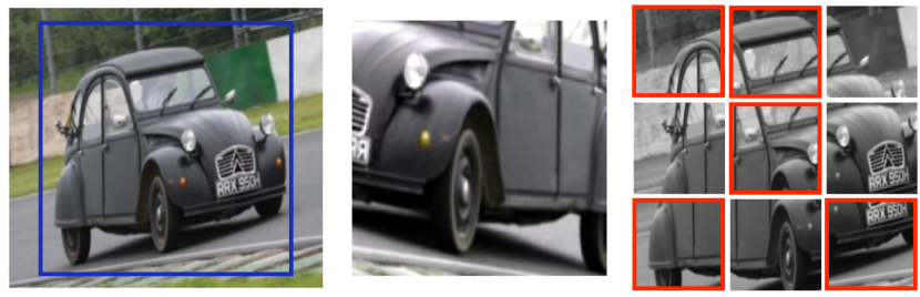
Figure 4: Reconstructing BoWs from small parts of the original image. Given a training image (left), we extract two types of image crops. The first type (middle) is obtained by randomly sampling an image region whose area covers no more than $60\%$ of the entire image, resizing it to $160\times 160$ and then giving it as input to the student as part of the reconstruction task. The second type (right) is obtained by randomly selecting an area that covers between $60\%$ to $100\%$ of the entire image, resizing it to a $256\times 256$ image, dividing it into $3\times 3$ overlapping patches of size $96\times 96$, and randomly choosing $5$ out of these $9$ patches (indicated with red rectangles) that are given as $5$ separate inputs to the student. The student must then reconstruct the original BoW target independently for each patch. The blue rectangle on the left image indicates the central $224\times 224$ crop from which the teacher produces the BoW target. Note that, except from horizontal flipping, no other perturbation is applied on the teacher’s inputs.

Multi-scale BoW reconstruction targets.   We also consider reconstructing BoW from multiple network layers that correspond to different scale levels. In particular, we experiment with using both the last scale level $L$ (i.e., layer conv5 in ResNet) and the penultimate scale level $L\!-\!1$ (i.e., layer conv4 in ResNet). The reasoning behind this is that the features of level $L\!-\!1$ still encode semantically important concepts but have a smaller receptive field than those in the last level. As a result, the visual words of level $L\!-\!1$ that belong to image regions hidden to the student are less likely to be influenced by pixels of image regions the student is given as input. Therefore, by using BoW from this extra feature level, the student is further enforced to learn contextual reasoning skills (and in fact, at a level with higher spatial details due to the higher resolution of level $L\!-\!1$), thus learning richer and more powerful representations. When using BoW extracted from two layers, our method includes a separate vocabulary for each layer, denoted by $V_{L}$ and $V_{L-1}$ for layers $L$ and $L\!-\!1$ respectively, and two different weight generators, denoted by $\mathrm{G}_{L}(\cdot)$ and $\mathrm{G}_{L\!-\!1}(\cdot)$ for layers $L$ and $L\!-\!1$, respectively. Regardless of what layer the BoW target comes from, the student uses a single global image representation $\mathrm{S}(\tilde{\mathbf{x}})$, typically coming from the global average pooling layer after the last convolutional layer (i.e., layer pool5 in ResNet), to perform the reconstruction task.

We show empirically in Section 4.1 that the contextual reasoning skills implicitly developed via using the above two schemes are decisive to learn effective image representations with the BoW-reconstruction task.

4 Experiments and results

We evaluate our method (OBoW) on the ImageNet [64], Places205 [87] and VOC07 [22] classification datasets as well as on the V0C07+12 detection dataset.

Implementation details.   For our models, the vocabulary size is set to $K=8192$ words and, as in BoWNet, when computing the BoW targets we ignore the visual words that correspond to the feature vectors on the edge of the teacher feature maps. The momentum coefficient $\alpha$ for the teacher updates is initialized at $0.99$ and is annealed to $1.0$ during training with a cosine schedule. The hyper-parameters $\kappa$ and $\delta_{\rm base}$ are set to $5$ and $1/10$ respectively for the results in § 4.1, to $8$ and $1/15$ respectively for the results in § 4.3. For more implementation details see § C.

4.1 Analysis

Here we perform a detailed analysis of our method. Due to the computationally intensive nature of pre-training on ImageNet, we use a smaller but still representative version created by keeping only $20\%$ of its images and we implement our model with the light-weight ResNet18 architecture. For training we use SGD for $80$ epochs with cosine learning rate initialized at $0.05$, batch size $128$ and weight decay $5\mathrm{e-}4$. We evaluate models trained with two versions of our method, the vanilla version that uses single-scale BoWs and from each training image extracts one $160\times 160$-sized crop (with which it trains the student), and the full version that uses multi-scale BoWs and extracts from each training image two $160\times 160$-sized crops plus five $96\times 96$-sized patches.

Evaluation protocols.   After pre-training, we freeze the learned representations and use two evaluation protocols. (1) The first one consists in training $1000$-way linear classifiers for the ImageNet classification task. (2) For the second protocol, our goal is to analyze the ability of the representations to learn with few training examples. To that end, we use $300$ ImageNet classes and run with them multiple ($200$) episodes of $50$-way classification tasks with $1$ or $5$ training examples per class and a Prototypical-Networks [67] classifier.

4.2 Results

	Few-shot
Updating method	1-shot	5-shot	Linear
Online k-means
(a) replacing rare clusters	40.98	60.35	44.45
(b) Sinkhorn-based balancing	37.20	55.22	39.74
Queue-based vocabulary
(a) local features	40.29	60.81	44.39
(b) globally-averaged features	41.57	62.54	45.79
(c) locally-averaged features	42.11	62.44	45.86
Queue-based vocabulary – multi-scale BoW
(b) globally-averaged features	41.29	63.09	49.40
(c) locally-averaged features	44.18	64.89	50.89

Table 1: Comparison of online vocabulary-update approaches. The results in the first two sections are with the vanilla version of our method and with the full version in the third section.

Online vocabulary updates.   In Tab. 1, we compare the approaches for online vocabulary updates described § 3.1. The queue-based solutions achieve in general better results than online k-means. Among the queue-based options, random sampling of locally averaged features, opt. (c), provides the best results. Its advantage over option (b) with global averaging is more evident with multi-scale BoWs where an extra feature level with a higher resolution and more localized features is used, in which case global averaging produces visual words that are too coarse. In all remaining experiments, we use a queue-based vocabulary with option (c).

Momentum for teacher updates.   In Table 2, we study the sensitivity of our method w.r.t. the momentum $\alpha$ for the teacher updates (Equation 3). We notice a strong drop in performance when decreasing $\alpha$ from $0.9$ to $0.5$ (a rapidly-changing teacher), and to $0$ (the teacher and student have identical parameters), while keeping the initial learning rate fixed ($lr=0.05$). However, we noticed that this was not due to any cluster/mode collapse issue. The issue is that the teacher signal is more noisy at low $\alpha$ because of the rapid change of its parameters. This prevents the student to converge when keeping the learning rate as high as $0.05$. We notice in Table 2 that a reduction of the learning rate to adapt to the reduction of $\alpha$ reduces the performance gap. This indicates that our method is not as sensitive to the choice of the momentum as MoCo and BYOL were shown to be.

		Few-shot
$\alpha$	lr	1-shot	1-shot	Linear
$0.99\rightarrow 1$	$0.05$	42.11	62.44	45.86
$0.999$	$0.05$	40.87	61.41	45.76
$0.99$	$0.05$	41.19	61.65	46.25
$0.9$	$0.05$	40.79	60.92	44.89
$0.5$	$0.05$	12.70	23.20	15.41
$0.0$	$0.05$	13.19	24.85	17.47
$0.5$	$0.03$	39.52	60.18	43.82
$0.0$	$0.01$	33.80	55.02	39.90

Table 2: Influence of the momentum coefficient $\alpha$ used for the teacher updates. For these results, we used the vanilla version. In the “$0.99\rightarrow 1$” row, $\alpha$ is initialized to $0.99$ and annealed to $1.0$ with cosine schedule. The other entries use constant $\alpha$ values.

		Few-shot
Soft	Dyn	1-shot	5-shot	Linear
✓	✓	42.11	62.44	45.86
	✓	38.61	59.98	44.64
✓		2.00	2.00	0.10

Table 3: Ablation of dynamic BoW prediction and soft-quantization. For these results, we used the vanilla version of our method. “Soft”: soft assignment instead of hard assignment. “Dyn”: dynamic weight generation instead of fixed weights.

Image crops	Multi-scale	Linear
$1\times 224^{2}$		31.39
$1\times 224^{2}$ + cutmix		39.46
$1\times 160^{2}$		45.86
$2\times 160^{2}$		47.64
$5\times 96^{2}$		44.24
$2\times 160^{2}$ + $5\times 96^{2}$		49.64
$2\times 160^{2}$	✓	49.00
$2\times 160^{2}$ + $5\times 96^{2}$	✓	50.89

Table 4: Evaluation of image crop augmentations and of multi-scale BoWs. See text.

		Few-shot
Method	EP	$n=1$	$n=5$	Linear
BoWNet	200	33.80	55.02	41.30
BoWNet ($160^{2}$ crops)	200	29.26	49.68	43.59
OBoW (vanilla)	80	42.11	62.44	45.86
OBoW (full)	80	44.18	64.89	50.89

Table 5: Comparison with BoW-like methods. “EP”: total number of epochs used for pre-training. Note that the BoWNet method consists of $40$ epochs for teacher pre-training with the RotNet method followed by two BoWNet training rounds of $80$ epochs.

			Linear Classification			VOC Detection			Semi-supervised learning
Method	Epochs	Batch	ImageNet	Places205	VOC07	$\text{AP}^{\text{50}}$	$\text{AP}^{75}$	$\text{AP}^{\text{all}}$	$1\%$ Labels	$10\%$ Labels
Supervised	100	256	76.5	53.2	87.5	81.3	58.8	53.5	48.4	80.4
BoWNet [26]	325	256	62.1	51.1	79.3	81.3	61.1	55.8	-	-
PCL [48]	200	256	67.6	50.3	85.4	-	-	-	75.3	85.6
MoCo v2 [35]	200	256	67.5	-	-	82.4	63.6	57.0	-	-
SimCLR [9]	200	4096	66.8	-	-	-	-	-	-	-
SwAV [8]	200	256	72.7	56.2†	87.2†	81.8†	60.0†	54.4†	76.7†	88.7†
BYOL [33]	300	4096	72.5	-	-	-	-	-	-	-
OBoW (Ours)	200	256	73.8	56.8	89.3	82.9	64.8	57.9	82.9	90.7
PIRL [51]	800	1024	63.6	49.8	81.1	80.7	59.7	54.0	57.2	83.8
MoCo v2 [35]	800	256	71.1	52.9	87.1	82.5	64.0	57.4	-	-
SimCLR [9]	1000	4096	69.3	53.3	86.4	-	-	-	75.5	87.8
BYOL [33]	1000	4096	74.3	-	-	-	-	-	78.4	89.0
SwAV [8]	800	4096	75.3	56.5	88.9	82.6	62.7	56.1	78.5	89.9

Table 6: Evaluation of ImageNet pre-trained ResNet50 models. The “Epochs” and “Batch” columns provide the number of pre-training epochs and the batch size of each model respectively. The first section includes models pre-trained with a similar number of epochs as our model (second section). We boldfaced the best results among all sections as well as of only the top two. For the linear classification tasks, we provide the top-1 accuracy. For object detection, we fine-tuned Faster R-CNN (R50-C4) on VOC trainval07+12 and report detection AP scores by testing on test07. For semi-supervised learning, we fine-tune the pre-trained models on $1\%$ and $10\%$ of ImageNet and report the top-5 accuracy. Note that, in this case the “Supervised” entry results come from [83] and are obtained by supervised training using only $1\%$ or $10\%$ of the labelled data. All the classification results are computed with single-crop testing. ^†: results computed by us.

Dynamic BoW prediction and soft quantization.   In Table 3, we study the impact of the dynamic BoW prediction and of using soft assignment for the codes instead of hard assignment. We see that (1), as expected, the network is unable to learn useful features without the proposed dynamic BoW prediction, i.e., when using fixed weights; (2) soft assignment indeed provides a performance boost.

Enforcing context-aware representations.   In Table 4 we study different types of image crops for the BoW reconstruction tasks, as well as the impact of multi-scale BoW targets. We observe that: (1) as we discussed in § 3.3, smaller crops that hide significant portions of the original image are better suited for our reconstruction task thus leading to dramatic increase in performance (compare entries $1\times 224^{2}$ with the $1\times 160^{2}$ and $5\times 96^{2}$ entries). (2) Randomly sampling two $160\times 160$-sized crops (entries $2\times 160^{2}$) and using $96\times 96$-sized patches leads to another significant increase in performance. (3) Finally, employing multi-scale BoWs improves the performance even further.

BoW-like comparison.   In Table 5, we compare our method with the reference BoW-like method BoWNet. For a fair comparison, we implemented BoWNet both with its proposed augmentations, i.e., using one $224\times 224$-sized crop with cutmix (“BoWNet” row), and with the image augmentation we propose in the vanilla version of our method, i.e., one $160\times 160$-sized crop (“BoWNet ($160^{2}$ crops)”). We see that our method, even in its vanilla version, achieves significantly better results, while using at least two times fewer training epochs, which validates the efficiency of our proposed fully-online training methodology.

4.3 Self-supervised training on ImageNet

Here we evaluate our method by pre-training with it convnet-based representations on the full ImageNet dataset. We implement the full solution of our method (as described in § 4.1) using the ResNet50 (v1) [37] architecture. We evaluate the learned representations on ImageNet, Places205, and VOC07 classification tasks as well as on VOC07+12 detection task and provide results in Table 6. On the ImageNet classification we evaluate on two settings: (1) training linear classifiers with $100\%$ of the data, and (2) fine-tuning the model using $1\%$ or $10\%$ of the data, which is referred to as semi-supervised learning.

Results.   Pre-training on the full ImageNet and then transferring to downstream tasks is the most popular benchmark for unsupervised representations and thus many methods have configurations specifically tuned on it. In our case, due to the computational intensive nature of pre-training on ImageNet, no full tuning of OBoW took place. Nevertheless, it achieves very strong empirical results across the board. Its classification performance on ImageNet is $73.8\%$, which is substantially better than instance discrimination methods MoCo v2 and SimCLR, and even improves over the recently proposed BYOL and SwAV methods when considering a similar amount of pre-training epochs. Moreover, in VOC07 classification and Places205 classification, it achieves a new state of the art despite using significantly fewer pre-training epochs than related methods. On the semi-supervised ImageNet ResNet50 setting, it significantly surpasses the state of the art for $1\%$ labels, and is also better for $10\%$ labels using again much fewer epochs. On VOC detection, it outperforms previous state-of-the-art methods while demonstrating strong performance improvements over supervised pre-training.

5 Conclusion

In this work, we introduce OBoW, a novel unsupervised teacher-student scheme that learns convnet-based representations with a BoW-guided reconstruction task. By employing an efficient fully-online training strategy and promoting the learning of context-aware representations, it delivers strong results that surpass prior state-of-the-art approaches on most evaluation protocols. For instance, when evaluating the derived unsupervised representations on the Places205 classification, Pascal classification or Pascal object detection tasks, OBoW attains a new state of the art, surpassing prior methods while demonstrating significant improvements over supervised representations.

Appendix A Comparing with MoCo for the same image augmentations

In the main paper we saw that the image augmentation techniques that we designed for our method have a strong positive impact on the quality of the learned representations. However, we stress that the performance improvement of our method over state-of-the-art instance-discrimination methods is not simply due a better mix of augmentations.

For example, in Table 7 we compare OBoW with MoCo v2, when the latter is implemented with the same image augmentations as those in the full solution of OBoW. We see that indeed, although the proposed augmentations also improve MoCo v2, our method is still significantly better, even in its vanilla version that employs simpler augmentations (i.e., only a single $160\times 160$-sized crop). Therefore, the ability of OBoW to learn state-of-the-art representations is mainly due to its BoW-guided reconstruction formulation.

Appendix B Visualization of the vocabulary features

In Figures 5 and  6 we illustrate visual words from the conv5 and conv4 teacher feature maps of a ResNet50 OBoW model trained on ImageNet. Since we use a queue-based vocabulary that is constantly updated, for the visualizations we used the state of the vocabulary at the end of training. In order to visualize a visual word, we retrieve multiple image patches from images in the ImageNet training set and depict the 8 patches with the highest assignment score for that visual word. As it can be noticed, visual words encode high level visual concepts.

		Few-shot
Method	EP	$n=1$	$n=5$	Linear
OBoW (vanilla)	80	42.11	62.44	45.86
OBoW (full)	80	44.18	64.89	50.89
MoCo v2	80	24.75	43.89	35.00
MoCo v2 (our aug.)	80	36.90	55.87	43.13

Table 7: Comparison with MoCo v2 for the same image augmentations. “EP”: total number of epochs used for pre-training. The results are obtained by training ResNet18-based models on $20\%$ of ImageNet, similar to Sections 4.1 and 4.2 of the main paper. “MoCo v2 (our aug.) ” is a MoCo v2 model implemented with the same augmentations that we use in the full version of our work, i.e., two $160\times 160$-sized crops plus five $96\times 96$-sized patches.

Figure 5: Examples of visual-word members from the conv5 layer of ResNet50. The visualizations are created by using the state of the queue-based visual-words vocabulary at the end of training. For each visual word, we depict the 8 image patches retrieved from ImageNet with the highest assignment score for that word.

Figure 6: Examples of visual-word members from the conv4 layer of ResNet50. The visualizations are created by using the state of the queue-based visual-words vocabulary at the end of training. For each visual word, we depict the 8 image patches retrieved from ImageNet with the highest assignment score for that word.

Appendix C Implementation details

C.1 Image augmentation during pre-training

In Section 3.3 of the main paper, we described the two types of image crops that we extract from a training image in order to train the student network with them. In addition, beyond image cropping, similar to SimCLR [9], we also applied color jittering, color-to-grayscale conversion, Gaussian blurring and horizontal flipping as augmentation techniques. All implementation details are provided in Section G in the form of PyTorch code.

C.2 Evaluation protocols in Section 4.1

To evaluate the quality of the learned representations, we use two protocols. (1) The first protocol consists in freezing the convnet and then training on its features $1000$-way linear classifiers for the ImageNet classification task. The classifier is applied on top of the $512$-dimensional feature vectors produced from the final global pooling layer of ResNet18. It is trained with SGD for $50$ epochs using a learning rate of $10$ that is divided by a factor of $10$ every $15$ epochs. The batch size is $256$ and the weight decay $2\rm e{-}6$. For fast experimentation, we train the linear classifier with precached features extracted from the $224\times 224$ central crop of the image and its horizontally flipped version. (2) For the second protocol, we use a few-shot episodic setting [75]. We choose $300$ classes from ImageNet and run $200$ episodes of $50$-way few-shot classification tasks. Essentially, for each episode, we randomly select $50$ classes from the $300$ ones and, for each of these selected classes, $n$ training examples and $m=1$ test example (both randomly sampled from the validation images of ImageNet). For $n$, we use $1$ and $5$ examples corresponding to $1$-shot and $5$-shot classification settings, respectively. The $m$ test examples per class are classified using a cosine-distance Prototypical-Networks [67] classifier applied on top of the frozen self-supervised representations. We report the mean accuracy over the $200$ episodes. The purpose of this metric is to analyze the ability of the representations to be used for learning with few training examples. Furthermore, it has the advantage of not requiring tuning of any hyper-parameters, such as the learning rate of a linear classifier, the number of training steps, etc.

C.3 Self-supervised training on ImageNet

Here we provide implementation details for the pre-training of the ResNet50-based OBoW model that we use in Section 4.3 of the main paper. We present the full implementation of our method, which includes multi-scale BoWs from the conv4 and conv5 layers of ResNet50, and extraction of two crops of size $160\times 160$ plus five patches of size $96\times 96$ per training image. To extract BoW targets, we use $K=8192$ as vocabulary size and we ignore the local feature vectors on the edge / border of the teacher’s feature maps. The momentum coefficient $\alpha$ for the teacher updates is initialized at $0.99$ and is annealed to $1.0$ during training with a cosine schedule. Finally, the hyper-parameters $\kappa$ and $\delta_{\mathrm{base}}$ are set to $8$ and $1/15$ respectively.

We train the model for $200$ training epochs with SGD using $1\rm e{-}4$ weight decay and $256$-sized mini-batches. As a learning-rate schedule, we warm up the learning rate from $0$ to $0.03$ with linear annealing during the first $10$ epochs and then, for the remaining $190$ epochs, we decrease it from $0.03$ to $0.00003$ with cosine-based schedule. To train the model we use 4 Tesla V100 GPUs with data-distributed training (i.e., the mini-batch is divided across the 4 GPUs) while keeping the batch-norm statistics synchronized across all GPUs (i.e., use the SyncBatchNorm units of PyTorch).

C.4 Evaluation protocols in Section 4.3

Here we describe the evaluation protocols that we use in Section 4.3 of the main paper.

ImageNet linear classification.   In this case, we evaluate the performance on the $1000$-way ImageNet classification task by applying a linear classifier on top of the $2048$-dimensional frozen features of the pool5 layer of ResNet50. We train the linear classifier using SGD for $100$ training epochs with $0.9$ momentum, $0$ weight decay, $1024$-sized mini-batches and cosine learning-rate schedule initialized at $10.0$. We use the typical image augmentations used for the fully-supervised training of ResNet50 models on this dataset.

Places205 linear classification.   For this protocol, we evaluate the performance on the $205$-way Places classification task by applying a linear classifier on top of the $2048$-dimensional frozen features of the pool5 layer of ResNet50. We follow the guidelines of [32] and train the linear classifier using SGD for $14$ training epochs and a learning rate of $0.01$ that is multiplied by $0.1$ after $5$ and $10$ epochs. The batch size is $256$ and the weight decay is $1\rm e{-}4$.

VOC07 linear classification with SVMs.   Here we evaluate on the VOC07 classification task by training and testing linear SVMs on top of the $2048$-dimensional frozen features of the pool5 layer. To this end, we use the publicly available code for benchmarking self-supervised methods provided in [32] that trains the SVMs using the VOC07 train+val splits and tests them using the VOC07 test split.

Semi-supervised learning setting on ImageNet.   For this semi-supervised setting, we fine-tune the self-supervised ResNet50 model (pre-trained on all ImageNet unlabelled images) on $1\%$ or $10\%$ of ImageNet labelled images. We use the same $1\%$ and $10\%$ splits as in SimCLR (i.e., we downloaded and use the split files of their official code release). We train using SGD with $256$-sized mini-batches, $0$ weight decay, and two distinct learning rates for the classification head and the feature extractor trunk network components respectively. Specifically, in the $1\%$ setting, we use $40$ epochs and the initial learning rates $0.5$ and $0.0002$ for the classification head and feature extractor trunk components, respectively, which are then multiplied by a factor of $0.2$ after $24$ and $32$ epochs. In the $10\%$ setting, we use $20$ epochs and the initial learning rates $0.5$ and $0.0002$ for the classification head and feature extractor trunk components, respectively, which are multiplied by a factor of $0.2$ after $12$ and $16$ epochs.

VOC object detection.   Here we evaluate the utility of OBoW on a complex downstream task: object detection. We follow the setup considered in prior works [8, 26, 32, 35, 51]: we fine-tune the pre-trained OBoW with a Faster R-CNN [63] model using a ResNet50 backbone [36] (R50-C4 in Detectron2 [79]). We use the fine-tuning protocol and most hyper-parameters from He et al. [35]: fine-tune on trainval07+12 and evaluate on test07. In detail, we train with mini-batches of size $16$ across $4$ GPUs for $24$K steps, using SyncBatchNorm to finetune BatchNorm parameters, as well as inserting an additional BatchNorm layer for the RoI head after conv5, i.e., Res5ROIHeadsExtraNorm layer in Detectron2. The initial learning rate $0.01$ is warmed-up with a slope of $1\rm e{-}3$ for $100$ steps and then reduced by a factor of $10$ after $18$K and $22$K steps. We report results for the final checkpoint averaged over 3 different runs.

Appendix D On-line k-means vocabulary updates

As explained in the main paper, one of the explored choices for updating the vocabulary is to use online k-means after each training step. Specifically, as proposed in VQ-VAE [55, 62], we use exponential moving average for vocabulary updates. In this case, for each mini-batch, we compute the number $n_{k}$ of feature vectors assigned to each cluster $k$ and $\mathbf{m}_{k}$ the element-wise sum of all feature vectors assigned to cluster $k$ and update

$$N_{k} \leftarrow\gamma N_{k}+(1-\gamma)n_{k},$$ (6)

$$\mathbf{M}_{k} \leftarrow\gamma\mathbf{M}_{k}+(1-\gamma)\mathbf{m}_{k},$$ (7)

with $\gamma=0.99$. The $k^{\rm th}$ visual word of the vocabulary $V$ satisfies $\mathbf{v}_{k}={\mathbf{M}_{k}}/{N_{k}}$. A critical issue that arises in this case is that, as training progresses, the features distribution changes over time. The visual words computed by online k-means do not adapt to this distribution shift leading to extremely unbalanced cluster assignments and even to assignments that collapse to a single cluster. In order to counter this effect, we investigate two different strategies:

(a) Detection and replacement of rare visual words.   In this case, for each visual word we keep track of the time of its most recent assignment as closest cluster centroid to a feature vector. If more than $1000$ training steps have passed since then, then we replace it with a local feature vector randomly sampled with uniform distribution from the current mini-batch.

(b) Enforcing uniform assignments via Sinkhorn optimization.   Let $\mathbf{x}_{1},\ldots,\mathbf{x}_{b}$ be the $b$ images of the current mini-batch and $D$ be the $K\times B$ matrix ($B=h_{\ell}\times w_{\ell}\times b$) whose $i^{\rm th}$ row $D_{i}$ contains the squared distances between all the local features in the mini-batch (across all images and spatial dimensions) and the $i^{\rm th}$ visual word: $D_{i}=\big{[}\,\|\mathrm{T}(\mathbf{x}_{1})[1]-\mathbf{v}_{i}\|_{2}^{2},\ldots,\|\mathrm{T}(\mathbf{x}_{b})[h_{\ell}\times w_{\ell}]-\mathbf{v}_{i}\|_{2}^{2},\big{]}$. Similarly to [4, 8], we compute the assignment codes by solving the regularised optimal transport problem $\min_{Q\in\mathcal{Q}}\sum_{i,j}Q_{i,j}D_{i,j}+\varepsilon\,Q_{i,j}\log Q_{i,j}$, where $\varepsilon$ is a coefficient that controls the softness of the assignments. The set $\mathcal{Q}$ permits us to enforce uniform assignments among all the visual words and satisfies $\mathcal{Q}=\{Q\in\mathbb{R}_{+}^{K\times B}|Q\mathbf{1}_{B}=\frac{1}{K}\mathbf{1}_{K},Q^{\top}\mathbf{1}_{K}=\frac{1}{B}\mathbf{1}_{B}\}$, where $\mathbf{1}_{K}$ and $\mathbf{1}_{B}$ are vectors of length $K$ and $B$, respectively, with all entries equal to $1$. We compute $Q$ with the Sinkhorn algorithm [14] and use the resulting assignment codes for the on-line k-means updates and for the computation of the BoW targets.

	Sup.	OBoW	MoCo v2	BYOL
Epochs	100	200	800	300
Measured with $256$-sized mini-batches
Time per epoch	1.00	3.91	1.58	3.47
Training time	1.00	7.82	12.64	10.41
Memory per GPU	1.00	2.00	1.13	1.72
ImageNet linear classification accuracy
batch size = $256$	76.5	73.8	71.1	-
batch size = $4096$	-	-	-	72.5†

Table 8: Time and memory consumption relative to supervised training. “Sup.” is the supervised ImageNet training. To measure the time and memory consumption, for all methods we used ResNet50-based implementations, $256$-sized mini-batches and data-distributed training with 4 Tesla V100 GPUs. We measured the time consumption based on a single training epoch (“Time per epoch”). We also provide the projected time for the full training of a method (“Training time”), which is estimated based on the specified number of training epochs (“Epochs”). For OBoW, we used its full implementation. ^†: for BYOL we provide the time and memory consumption w.r.t. $256$-sized mini-batches, but BYOL uses $4096$-sized mini-batches to achieve the reported ImageNet classification accuracy. So, in reality BYOL has higher total GPU memory requirements.

Appendix E Time and memory consumption

In Table 8, we provide the time and memory consumption of our method as well as of MoCo v2 and BYOL. We observe that OBoW achieves state-of-the-art results in less time (“Training time” row) than the competing methods. In terms of GPU memory consumption, with $256$-sized mini-batches our method requires $15775$Mb per GPU in a 4-GPU machine (or $8901$Mb per GPU in a 8-GPU machine).

Appendix F COCO detection and instance segmentation

In Table 9 we evaluate the learned representations on the downstream tasks of object detection and instance segmentation on COCO [50]. To this end, we fine-tune the pre-trained representations with a Mask R-CNN [36] model with a ResNet50 backbone and feature pyramid networks [49] (Mask R-CNN R50-FPN) implemented in Detectron2. We train the Mask R-CNN model on train2017 for $12$ epochs ($1\times$ schedule) and report the box detection AP (AP${}^{\text{bb}}_{\text{~{}}}$) and instance segmentation AP (AP${}^{\text{mk}}_{\text{~{}}}$) on COCO val2017. Similar to VOC detection experiments, BatchNorm layers are fine-tuned and synchronized. We see that OBoW achieves better or comparable results to prior methods despite the fact that it used only 200 pre-training epochs.

method	Epochs	Batch	AP${}^{\text{bb}}_{\text{~{}}}$	AP${}^{\text{mk}}_{\text{~{}}}$
Supervised	100	256	39.6	35.6
VADeR [60]	600	128	39.2	35.6
SimCLR [9]	1000	4096	39.7	35.8
MoCo v2 [11]	800	256	40.4	36.4
InfoMin [70]	200	256	40.6	36.7
BYOL [33]	1000	4096	41.6	37.2
SwAV [8]	800	4096	41.6	37.8
OBoW (ours)	200	256	40.8	36.4

Table 9: Results of object detection and instance segmentation on COCO. We report the box detection AP (AP${}^{\text{bb}}_{\text{~{}}}$) and instance segmentation AP (AP${}^{\text{mk}}_{\text{~{}}}$) on val2017. All methods are pretrained on ImageNet and then fined-tuned on COCO for $12$ epochs ($1\times$ schedule). We use the ResNet50-based Mask-RCNN model equipped with feature pyramid networks (Mask R-CNN R50-FPN). The “Epochs” and “Batch” columns provide the number of pre-training epochs and the batch size of each model respectively.

Appendix G PyTorch code of Image augmentations

Here we provide the PyTorch implementation of the image augmentations used in our work.

⬇

1import random

2import torch

3import torchvision.transforms as T

4from PIL import ImageFilter

5

6class CropImagePatches:

7 """Crops from an image 3 x 3 overlapping patches."""

8 def __init__(self, patch_size=96, patch_jitter=24, num_patches=5):

9 self.patch_size = patch_size

10 self.patch_jitter = patch_jitter

11 self.num_patches = num_patches

12

13 def __call__(self, img):

14 _, height, width = img.size()

15 split_per_side = 3

16 offset_y = (height - self.patch_size - self.patch_jitter) // (split_per_side-1)

17 offset_x = (width - self.patch_size - self.patch_jitter) // (split_per_side-1)

18

19 patches = []

20 for i in range(split_per_side):

21 for j in range(split_per_side):

22 y_top = i * offset_y + random.randint(0, self.patch_jitter)

23 x_left = j * offset_x + random.randint(0, self.patch_jitter)

24 y_bottom = y_top + self.patch_size

25 x_right = x_left + self.patch_size

26 patches.append(img[:, y_top:y_bottom, x_left:x_right])

27

28 if self.num_patches < (split_per_side * split_per_side):

29 indices = torch.randperm(len(patches))[:self.num_patches]

30 patches = [patches[i] for i in indices.tolist()]

31

32 return torch.stack(patches, dim=0)

33

34class StackMultipleViews:

35 def __init__(self, transform, num_views):

36 self.transform = transform

37 self.num_views = num_views

38

39 def __call__(self, img):

40 return torch.stack([self.transform(img) for _ in range(self.num_views)], dim=0)

41

42class GaussianBlur:

43 def __init__(self, sigma=[.1, 2.]):

44 self.sigma = sigma

45

46 def __call__(self, img):

47 sigma = random.uniform(self.sigma[0], self.sigma[1])

48 return img.filter(ImageFilter.GaussianBlur(radius=sigma))

49

50normalize = T.Normalize(mean=[0.485, 0.456, 0.406], std=[0.229, 0.224, 0.225])

51

52# Define the transformations for extracting the central from of the original image.

53transform_original_image = T.Compose([

54 T.Resize(256),

55 T.CenterCrop(224),

56 T.RandomHorizontalFlip(),

57 T.ToTensor(),

58 normalize])

59

60# Define the transformations for generating two 160x160-sized image crops.

61transform_two_160x160_image_crops = StackMultipleViews(

62 transform=T.Compose([

63 T.RandomResizedCrop(160, scale=[0.08, 0.6]),

64 T.RandomApply([T.ColorJitter(0.4, 0.4, 0.4, 0.1)], p=0.8),

65 T.RandomGrayscale(p=0.2),

66 T.RandomApply([GaussianBlur(sigma=[0.1, 2.0])], p=0.5),

67 T.RandomHorizontalFlip(),

68 T.ToTensor(),

69 normalize]),

70 num_views=2)

71

72# Define the transformations for generating two 160x160-sized image crops.

73transform_five_96x96_image_patches = T.Compose([

74 T.RandomResizedCrop(256, scale=[0.6, 1.0]),

75 T.RandomApply([T.ColorJitter(0.4, 0.4, 0.4, 0.1)], p=0.8),

76 T.RandomGrayscale(p=0.2),

77 T.RandomHorizontalFlip(),

78 T.ToTensor(),

79 normalize,

80 CropImagePatches(patch_size=96, patch_jitter=24, num_patches=5)])

References

- [1] Jean-Baptiste Alayrac, Joao Carreira, and Andrew Zisserman. The visual centrifuge: Model-free layered video representations. In CVPR, 2019.
- [2] Relja Arandjelovic, Petr Gronat, Akihiko Torii, Tomas Pajdla, and Josef Sivic. NetVLAD: CNN architecture for weakly supervised place recognition. In CVPR, 2016.
- [3] Relja Arandjelovic and Andrew Zisserman. Look, listen and learn. In ICCV, 2017.
- [4] Yuki Markus Asano, Christian Rupprecht, and Andrea Vedaldi. Self-labelling via simultaneous clustering and representation learning. In ICLR, 2020.
- [5] Cristian Bucilǎ, Rich Caruana, and Alexandru Niculescu-Mizil. Model compression. In KDD, 2006.
- [6] Mathilde Caron, Piotr Bojanowski, Armand Joulin, and Matthijs Douze. Deep clustering for unsupervised learning of visual features. In ECCV, 2018.
- [7] Mathilde Caron, Piotr Bojanowski, Julien Mairal, and Armand Joulin. Unsupervised pre-training of image features on non-curated data. In ICCV, 2019.
- [8] Mathilde Caron, Ishan Misra, Julien Mairal, Priya Goyal, Piotr Bojanowski, and Armand Joulin. Unsupervised learning of visual features by contrasting cluster assignments. In NeurIPS, 2020.
- [9] Ting Chen, Simon Kornblith, Mohammad Norouzi, and Geoffrey Hinton. A simple framework for contrastive learning of visual representations. In ICML, 2020.
- [10] Ting Chen, Xiaohua Zhai, Marvin Ritter, Mario Lucic, and Neil Houlsby. Self-supervised GANs via auxiliary rotation loss. In CVPR, 2019.
- [11] Xinlei Chen, Haoqi Fan, Ross Girshick, and Kaiming He. Improved baselines with momentum contrastive learning. arXiv, 2020.
- [12] Sumit Chopra, Raia Hadsell, and Yann LeCun. Learning a similarity metric discriminatively, with application to face verification. In CVPR, 2005.
- [13] Gabriella Csurka, Christopher Dance, Lixin Fan, Jutta Willamowski, and Cédric Bray. Visual categorization with bags of keypoints. In ECCVW, 2004.
- [14] Marco Cuturi. Sinkhorn distances: Lightspeed computation of optimal transport. In NeurIPS, 2013.
- [15] Arnaud Dapogny, Matthieu Cord, and Patrick Pérez. The missing data encoder: Cross-channel image completion with hide-and-seek adversarial network. In AAAI, 2020.
- [16] Carl Doersch, Abhinav Gupta, and Alexei Efros. Unsupervised visual representation learning by context prediction. In ICCV, 2015.
- [17] Jeff Donahue, Philipp Krähenbühl, and Trevor Darrell. Adversarial feature learning. In ICLR, 2017.
- [18] Jeff Donahue and Karen Simonyan. Large scale adversarial representation learning. In NeurIPS, 2019.
- [19] Alexey Dosovitskiy, Philipp Fischer, Jost Tobias Springenberg, Martin Riedmiller, and Thomas Brox. Discriminative unsupervised feature learning with exemplar convolutional neural networks. IEEE Trans. PAMI, 38(9), 2015.
- [20] Alexey Dosovitskiy, Jost Tobias Springenberg, Martin Riedmiller, and Thomas Brox. Discriminative unsupervised feature learning with convolutional neural networks. In NeurIPS, 2014.
- [21] Vincent Dumoulin, Ishmael Belghazi, Ben Poole, Olivier Mastropietro, Alex Lamb, Martin Arjovsky, and Aaron Courville. Adversarially learned inference. In ICLR, 2017.
- [22] Mark Everingham, Luc Van Gool, Chris Williams, John Winn, and Andrew Zisserman. The Pascal visual object classes (VOC) challenge. IJCV, 88(2), 2010.
- [23] William Falcon and Kyunghyun Cho. A framework for contrastive self-supervised learning and designing a new approach. arXiv, 2020.
- [24] Jonathan Frankle, David J Schwab, and Ari Morcos. Are all negatives created equal in contrastive instance discrimination? arXiv, 2020.
- [25] Elizabeth Gardner and Bernard Derrida. Three unfinished works on the optimal storage capacity of networks. Journal of Physics A: Mathematical and General, 22(12), 1989.
- [26] Spyros Gidaris, Andrei Bursuc, Nikos Komodakis, Patrick Pérez, and Matthieu Cord. Learning representations by predicting bags of visual words. In CVPR, 2020.
- [27] Spyros Gidaris and Nikos Komodakis. Dynamic few-shot visual learning without forgetting. In CVPR, 2018.
- [28] Spyros Gidaris, Praveer Singh, and Nikos Komodakis. Unsupervised representation learning by predicting image rotations. In ICLR, 2018.
- [29] Rohit Girdhar, Deva Ramanan, Abhinav Gupta, Josef Sivic, and Bryan Russell. ActionVLAD: Learning spatio-temporal aggregation for action classification. In CVPR, 2017.
- [30] Clément Godard, Oisin Mac Aodha, and Gabriel J Brostow. Unsupervised monocular depth estimation with left-right consistency. In CVPR, 2017.
- [31] Faustino Gomez and Jürgen Schmidhuber. Evolving modular fast-weight networks for control. In ICANN, 2005.
- [32] Priya Goyal, Dhruv Mahajan, Abhinav Gupta, and Ishan Misra. Scaling and benchmarking self-supervised visual representation learning. In ICCV, 2019.
- [33] Jean-Bastien Grill, Florian Strub, Florent Altché, Corentin Tallec, Pierre H Richemond, Elena Buchatskaya, Carl Doersch, Bernardo Avila Pires, Zhaohan Daniel Guo, Mohammad Gheshlaghi Azar, Bilal Piot, Koray Kavukcuoglu, Rémi Munos, and Michal Valko. Bootstrap your own latent: A new approach to self-supervised learning. In NeurIPS, 2020.
- [34] Raia Hadsell, Sumit Chopra, and Yann LeCun. Dimensionality reduction by learning an invariant mapping. In CVPR, 2006.
- [35] Kaiming He, Haoqi Fan, Yuxin Wu, Saining Xie, and Ross Girshick. Momentum contrast for unsupervised visual representation learning. In CVPR, 2020.
- [36] Kaiming He, Georgia Gkioxari, Piotr Dollár, and Ross Girshick. Mask R-CNN. In ICCV, 2017.
- [37] Kaiming He, Xiangyu Zhang, Shaoqing Ren, and Jian Sun. Deep residual learning for image recognition. In CVPR, 2016.
- [38] Olivier Henaff. Data-efficient image recognition with contrastive predictive coding. In ICML, 2020.
- [39] Geoffrey Hinton, Oriol Vinyals, and Jeff Dean. Distilling the knowledge in a neural network. In NIPSW, 2014.
- [40] Himalaya Jain, Spyros Gidaris, Nikos Komodakis, Patrick Pérez, and Matthieu Cord. QuEST: Quantized embedding space for transferring knowledge. In ECCV, 2020.
- [41] Ashish Jaiswal, Ashwin Ramesh Babu, Mohammad Zaki Zadeh, Debapriya Banerjee, and Fillia Makedon. A survey on contrastive self-supervised learning. arXiv, 2020.
- [42] Hervé Jégou, Matthijs Douze, Cordelia Schmid, and Patrick Pérez. Aggregating local descriptors into a compact image representation. In CVPR, 2010.
- [43] Yannis Kalantidis, Mert Bulent Sariyildiz, Noe Pion, Philippe Weinzaepfel, and Diane Larlus. Hard negative mixing for contrastive learning. In NeurIPS, 2020.
- [44] Anoop Korattikara Balan, Vivek Rathod, Kevin P Murphy, and Max Welling. Bayesian dark knowledge. In NeurIPS, 2015.
- [45] Samuli Laine and Timo Aila. Temporal ensembling for semi-supervised learning. In ICLR, 2017.
- [46] Gustav Larsson, Michael Maire, and Gregory Shakhnarovich. Learning representations for automatic colorization. In ECCV, 2016.
- [47] Hsin-Ying Lee, Jia-Bin Huang, Maneesh Singh, and Ming-Hsuan Yang. Unsupervised representation learning by sorting sequences. In ICCV, 2017.
- [48] Junnan Li, Pan Zhou, Caiming Xiong, Richard Socher, and Steven Hoi. Prototypical contrastive learning of unsupervised representations. In ICLR, 2021.
- [49] Tsung-Yi Lin, Piotr Dollár, Ross Girshick, Kaiming He, Bharath Hariharan, and Serge Belongie. Feature pyramid networks for object detection. In CVPR, 2017.
- [50] Tsung-Yi Lin, Michael Maire, Serge Belongie, James Hays, Pietro Perona, Deva Ramanan, Piotr Dollár, and C Lawrence Zitnick. Microsoft coco: Common objects in context. In ECCV. Springer, 2014.
- [51] Ishan Misra and Laurens van der Maaten. Self-supervised learning of pretext-invariant representations. In CVPR, 2020.
- [52] Ishan Misra, Lawrence Zitnick, and Martial Hebert. Shuffle and learn: unsupervised learning using temporal order verification. In ECCV, 2016.
- [53] Mehdi Noroozi and Paolo Favaro. Unsupervised learning of visual representations by solving jigsaw puzzles. In ECCV, 2016.
- [54] Aaron van den Oord, Yazhe Li, and Oriol Vinyals. Representation learning with contrastive predictive coding. arXiv, 2018.
- [55] Aaron van den Oord, Oriol Vinyals, and Koray Kavukcuoglu. Neural discrete representation learning. In NeurIPS, 2017.
- [56] George Papamakarios. Distilling model knowledge. arXiv, 2015.
- [57] Deepak Pathak, Philipp Krahenbuhl, Jeff Donahue, Trevor Darrell, and Alexei Efros. Context encoders: Feature learning by inpainting. In CVPR, 2016.
- [58] Florent Perronnin and Christopher Dance. Fisher kernels on visual vocabularies for image categorization. In CVPR, 2007.
- [59] Sudeep Pillai, Rareş Ambruş, and Adrien Gaidon. Superdepth: Self-supervised, super-resolved monocular depth estimation. In ICRA, 2019.
- [60] Pedro O Pinheiro, Amjad Almahairi, Ryan Y Benmalek, Florian Golemo, and Aaron Courville. Unsupervised learning of dense visual representations. In NeurIPS, 2020.
- [61] Siyuan Qiao, Chenxi Liu, Wei Shen, and Alan L Yuille. Few-shot image recognition by predicting parameters from activations. In CVPR, 2018.
- [62] Ali Razavi, Aaron van den Oord, and Oriol Vinyals. Generating diverse high-fidelity images with VQ-VAE-2. In NeurIPS, 2019.
- [63] Shaoqing Ren, Kaiming He, Ross Girshick, and Jian Sun. Faster R-CNN: Towards real-time object detection with region proposal networks. In NeurIPS, 2015.
- [64] Olga Russakovsky, Jia Deng, Hao Su, Jonathan Krause, Sanjeev Satheesh, Sean Ma, Zhiheng Huang, Andrej Karpathy, Aditya Khosla, Michael Bernstein, et al. Imagenet large scale visual recognition challenge. IJCV, 115(3), 2015.
- [65] David Saad and Sara A Solla. Dynamics of on-line gradient descent learning for multilayer neural networks. In NeurIPS, 1996.
- [66] Josef Sivic and Andrew Zisserman. Video google: Efficient visual search of videos. In Toward category-level object recognition. Springer, 2006.
- [67] Jake Snell, Kevin Swersky, and Richard Zemel. Prototypical networks for few-shot learning. In NeurIPS, 2017.
- [68] Antti Tarvainen and Harri Valpola. Mean teachers are better role models: Weight-averaged consistency targets improve semi-supervised deep learning results. In NeurIPS, 2017.
- [69] Yonglong Tian, Dilip Krishnan, and Phillip Isola. Contrastive multiview coding. In ECCV, 2020.
- [70] Yonglong Tian, Chen Sun, Ben Poole, Dilip Krishnan, Cordelia Schmid, and Phillip Isola. What makes for good views for contrastive learning. In NeurIPS, 2020.
- [71] Giorgos Tolias, Yannis Avrithis, and Hervé Jégou. To aggregate or not to aggregate: Selective match kernels for image search. In ICCV, 2013.
- [72] Trieu H Trinh, Minh-Thang Luong, and Quoc V Le. Selfie: Self-supervised pretraining for image embedding. arXiv, 2019.
- [73] Vikas Verma, Alex Lamb, Juho Kannala, Yoshua Bengio, and David Lopez-Paz. Interpolation consistency training for semi-supervised learning. In IJCAI, 2019.
- [74] Pascal Vincent, Hugo Larochelle, Yoshua Bengio, and Pierre-Antoine Manzagol. Extracting and composing robust features with denoising autoencoders. In ICML, 2008.
- [75] Oriol Vinyals, Charles Blundell, Tim Lillicrap, and Daan Wierstra. Matching networks for one shot learning. In NeurIPS, 2016.
- [76] Carl Vondrick, Abhinav Shrivastava, Alireza Fathi, Sergio Guadarrama, and Kevin Murphy. Tracking emerges by colorizing videos. In ECCV, 2018.
- [77] Tongzhou Wang and Phillip Isola. Understanding contrastive representation learning through alignment and uniformity on the hypersphere. In ICML, 2020.
- [78] Donglai Wei, Joseph J Lim, Andrew Zisserman, and William T Freeman. Learning and using the arrow of time. In CVPR, 2018.
- [79] Yuxin Wu, Alexander Kirillov, Francisco Massa, Wan-Yen Lo, and Ross Girshick. Detectron2, 2019.
- [80] Zhirong Wu, Yuanjun Xiong, Stella Yu, and Dahua Lin. Unsupervised feature learning via non-parametric instance-level discrimination. In CVPR, 2018.
- [81] Jun Yang, Yu-Gang Jiang, Alexander G Hauptmann, and Chong-Wah Ngo. Evaluating bag-of-visual-words representations in scene classification. In MIR, 2007.
- [82] Sangdoo Yun, Dongyoon Han, Seong Joon Oh, Sanghyuk Chun, Junsuk Choe, and Youngjoon Yoo. CutMix: Regularization strategy to train strong classifiers with localizable features. In ICCV, 2019.
- [83] Xiaohua Zhai, Avital Oliver, Alexander Kolesnikov, and Lucas Beyer. S4L: Self-supervised semi-supervised learning. In ICCV, 2019.
- [84] Liheng Zhang, Guo-Jun Qi, Liqiang Wang, and Jiebo Luo. AET vs. AED: Unsupervised representation learning by auto-encoding transformations rather than data. In CVPR, 2019.
- [85] Richard Zhang, Phillip Isola, and Alexei Efros. Colorful image colorization. In ECCV, 2016.
- [86] Richard Zhang, Phillip Isola, and Alexei Efros. Split-brain autoencoders: Unsupervised learning by cross-channel prediction. In CVPR, 2017.
- [87] Bolei Zhou, Agata Lapedriza, Jianxiong Xiao, Antonio Torralba, and Aude Oliva. Learning deep features for scene recognition using places database. In NeurIPS, 2014.
- [88] Tinghui Zhou, Matthew Brown, Noah Snavely, and David G Lowe. Unsupervised learning of depth and ego-motion from video. In CVPR, 2017.