Nonlinearity managed dissipative solitons

Abstract

We study the dynamics of localized pulses in the complex cubic-quintic Ginzburg-Landau (GL) equation with strong nonlinearity management. The generalized complex GL equation, averaged over rapid modulations of the nonlinearity, is derived. We employ the variational approach to this averaged equation to derive a dynamical system for the dissipative soliton parameters. By using numerical simulations of this dynamical system and the full GP equation, we show that nonlinearity-managed dissipative solitons exist in the model. The parameter regions for stabilization of exploding soliton are obtained.

1 Introduction

Dissipative solitons attract much attention nowadays due to a general importance for the theory of nonlinear waves and applications, such as mode-locked lasers, optical devices with gain/loss parameters, and other areas [1, 2]. In optics, a wide range of systems possessing dissipative solitons is described by the complex Ginzburg-Landau (GL) equation [1]. As many studies show, this equation has a rich variety of solutions, including stationary solitons, pulsating solitons, exploding solitons, and fronts (see e.g. [3]).

Pulsating solitons represent localized solutions with periodically or quasi-periodically varying amplitudes and widths. Pulsating solitons in the complex GL equation were found numerically in works [3, 4, 5]. Such solitons has been observed experimentally in fiber lasers [5]. It was shown that pulsating solitons are stable limit cycles (LC) of a finite dimensional dynamical system [6].

Exploding solitons(ES) are solitons with abrupt spreading and explosions of the pulse. Usually explosions are different from each other. After an explosion, a pulse has almost the same shape, though the pulse position can change. An interval between explosions and a shift of the pulse position seem to be random. Exploding solitons were observed experimentally in a sapphire laser [7], in a mode-locked fiber laser [8], and in an anomalous dispersion fiber laser [9].

Different schemes for stabilization and control of these pulses have been suggested. One of them is to take into account the higher-order effects. This leads to a formation of periodic, non-chaotic one-side explosions [10], and it can provide the shape stabilization of ESs [11]. Also, the dispersion management (DM) method, based on the rapid and strong variations of the dispersion on the evolutional variable, can be used to generate stable pulses with the enhanced energy. For dispersion-managed optical systems, some numerical results were obtained in works [12, 1], while an experiment was performed in Ref. [13]. In works [14, 15], the averaged GL equation has been derived. It was shown that the dispersion-managed GL equation is well approximated by the averaged over dispersion variations of nonlinear Schrödinger equation with the gain/loss terms of the same form as the original GL equation. The moments method has been applied to this problem in Ref. [16]. Mathematical aspects of the theory of dispersion managed optical solitons are discussed in the work  [17].

Another method that can be applied for soliton stabilization is the nonlinearity management (NM),which is based on the rapid and strong variations of the nonlinearity. For conservative systems, it was shown that nonlinearity management has many advantages for a generation of stable solitons in optical communication systems, in fiber lasers [18], and for generation of stable 2D spatial solitons [19, 20]. In attractive Bose-Einstein condensates (BECs), described by the focusing multi-dimensional nonlinear Schrödinger equation, the NM stabilization of solitons in BECs has been developed in Refs. [21, 22, 23, 24]. Therefore, it is of interest to study a possibility of dynamical stabilization of solitons in the complex cubic-quintic Ginzburg-Landau equation by the nonlinearity management.

In this work, we consider the dynamics of dissipative solitons in the complex cubic-quintic Ginzburg-Landau equation with a strong nonlinearity management. Such variations can be realized, for example, in a fiber ring laser with two-step (focusing and defocusing ) variations of nonlinearity.

The structure of the paper is as follows. In the Section 2, we describe a nonlinearity management model, and derive the generalized complex GL equation, averaged over the period of rapid modulations of nonlinearity. This complex GL equation is analyzed using the variational approach and the system of equations for dissipative soliton parameters is derived in Sec. 3. Results of numerical simulations of the system of variational equations for the pulse parameters and the full complex GL equation are given in Sec. 4. A possibility of stabilization of ES solutions is investigated also in this section.

2 The averaged complex GL equation

We consider the complex Ginzburg-Landau equation with nonlinearity management

$$iu_{t}+\frac{1}{2}u_{xx}+\gamma(t)|u|^{2}u+\chi|u|^{4}u=i\delta u+i\beta u_{xx}$$

$$+\ i\alpha|u|^{2}u+i\kappa|u|^{4}u\,,$$ (1)

where $\gamma(t)=\gamma_{0}+\gamma_{1}(t/\epsilon)/\epsilon$, and $\epsilon\ll 1.$ This equation models mode-locked lasers [25], long optical communication lines [26], and a soliton fiber lasers with two segments of alternating signs of nonlinearity [18]. In the case of passive mode-looked fiber lasers, $u$ is the normalized envelope of the field, $t$ is the propagation distance, $x$ is the number of trips (retarded time), $\gamma$ and $\chi$ correspond to the Kerr and saturating nonlinearities, $\delta$ is the linear gain (loss) coefficient, $\beta$ is the spectral filtering, and $\alpha$ and $\kappa$ describe nonlinear gain and absorption, respectively. We mention that a case of the rapidly varying dissipation in the framework of the nonlinear Schrodinger equation ($\chi=\alpha=\beta=\kappa=0$) is considered in Ref. [27].

We address here the case of periodic management $\gamma_{1}(\tau+1)=\gamma_{1}(\tau),\tau=t/\epsilon$ and $\int_{0}^{1}\gamma_{1}(\tau)d\tau=0$. We denote by $\Gamma_{1}$ the zero-mean antiderivative of $\gamma_{1}$ i.e.

$$\Gamma_{1}=\int_{0}^{\tau}\gamma_{1}(\tau)d\tau-\int_{0}^{1}d\tau\int_{0}^{\tau}\gamma_{1}(\tau^{\prime})d\tau^{\prime}.$$

Following the procedure developed in Refs. [28, 29], we average the complex Ginzburg-Landau equation over fast variations. Following these works, we represent field $u$ as the following

$$u=ve^{i\Gamma_{1}|v|^{2}}.$$ (2)

Substituting this transformation into Eq. (2) we obtain the following equation

$$iv_{t} - \Gamma_{1}v(|v|^{2})_{t}+\frac{1}{2}v_{xx}+\gamma_{0}|v|^{2}v$$ (3)

$$+ \chi|v|^{4}v+2i\Gamma_{1}(|v|^{2})_{x}v_{x}+i\Gamma_{1}(|v|^{2})_{xx}v-\Gamma_{1}^{2}(|v|^{2})_{x}v$$

$$= i\delta v+i\beta[v_{xx}+2i\Gamma_{1}(|v|^{2})_{x}v_{x}+i\Gamma_{1}(|v|^{2})_{xx}v$$

$$- \Gamma_{1}^{2}\left[(|v|^{2})_{x}\right]^{2}v]+i\alpha|v|^{2}v+i\kappa|v|^{4}v.$$

We consider that the solution depends on the fast time $\tau$ and the usual $T=t$. Looking for the solution

$$v(x,t)=w(x,T)+\epsilon v_{1}(x,\tau,T)+\epsilon^{2}v_{2}(x,\tau,T)+\dots$$

with $\epsilon\ll\beta,\alpha,\kappa$ and averaging over rapid oscillations we obtain the averaged complex Ginzburg-Landau equation for $w(x,t)$ (below we use notation $T\to t$)

$$iw_{t} + \frac{1}{2}w_{xx}+\gamma_{0}|w|^{2}w+\chi|w|^{4}w+\sigma^{2}\bigg{[}(|w|^{2})_{xx}|w|^{2}\bigg{.}$$ (4)

$$+ \frac{1}{2}(|w|_{x}^{2})^{2}\bigg{.}\bigg{]}w=R\equiv i\delta w+i\beta w_{xx}+i\alpha|w|^{2}w$$

$$+ i\kappa|w|^{4}w+i\beta\sigma^{2}(|w|^{2})_{x}w\bigg{[}2\left(w_{x}w^{\ast}-ww_{x}^{\ast}\right)\bigg{.}$$

$$- (|w|^{2})_{x}\bigg{.}\bigg{]}.$$

Here

$$\int_{0}^{1}d\tau\Gamma_{1}(\tau)=0,\int_{0}^{1}d\tau\Gamma_{1}^{2}(\tau)=\sigma^{2}.$$

Note that $\sigma^{2}\sim O(1)$, so we keep terms $\sim\sigma^{2}\beta$. In the case of weak management with $\sigma^{2}\ll 1$, these terms should be dropped [29].

Dissipative solitons exist when two balances are satisfied: the first one is the balance between nonlinearity and dispersion, and the second balance is between gain and loss. Comparing with the standard complex GL equation (Eq. 2 with $\gamma(t)=const$), we observe that two effects due to the nonlinearity management appear: the fourth order nonlinearity terms leading to the reduction of the nonlinearity [30], and the nonlinear renormalization of the filtering term $i\beta u_{xx}$. Thus, we can expect changes in the stability regions of dissipative solitons.

3 The system of equations for parameters of a nonlinearity managed dissipative soliton

For the conservative system ($\delta=\alpha=\beta=\kappa=0$), we have the Lagrangian density for Eq. (4)

$$L=\frac{i}{2}\bigg{(}w_{t}w^{\ast}-w^{\ast}w^{\ast}_{t}\bigg{)}-\frac{1}{2}|w_{x}|^{2}+\frac{\gamma_{0}}{2}|w|^{4}+\frac{\chi}{3}|w|^{6}-\frac{1}{2}\sigma^{2}|w|^{2}\left[(|w|^{2})_{x}\right]^{2}dx.$$ (5)

In order to derive the system of equations for the dissipative soliton parameters, we use the variational approach [31]. According to the variational approach, we should calculate the averaged Lagrangian

$$\bar{L}=\int_{-\infty}^{\infty}Ldx,$$

for a given ansatz for the wave profile $w(x,t)$. We will use the Gaussian ansatz for the dissipative soliton (DS) solution

$$w(x,t)=A(t)\exp\left\{-\frac{[x-x_{0}(t)]^{2}}{2a^{2}(t)}\right.$$

$$\Bigg{.}+ik(t)[x-x_{0}(t)]+ib(t)[x-x_{0}(t)]^{2}+i\phi(t)\Bigg{\}},$$ (6)

where $A(t),\ a(t)$ and $x_{0}$ are the amplitude, width and position of the pulse maximum, respectively, $k(t)$ is linear phase coefficient, $b(t)$ is the chirp parameter, and $\phi(t)$ is the phase shift. The Euler-Lagrange equations

$$\frac{\partial\bar{L}}{\partial\eta_{i}}-\frac{d}{dt}\frac{\partial\bar{L}}{\partial\eta_{i,t}}=\int_{-\infty}^{\infty}\left(\frac{\partial u^{\ast}}{\partial\eta_{i}}R+c.c.\right).$$ (7)

derived from the averaged Lagrangian, give a system of ordinary differential equations (ODEs) for the dissipative soliton parameters.

A calculation of the averaged Lagrangian $\bar{L}$ gives:

$$\frac{\bar{L}}{N}=-\frac{a^{2}b_{t}}{2}-\phi_{t}-\frac{1}{4a^{2}}-a^{2}b^{2}+\frac{\gamma_{0}N}{2\sqrt{2\pi}a}$$

$$+\frac{\chi N^{2}}{3\sqrt{3}\pi a^{2}}-\frac{\sigma^{2}N^{2}}{3\sqrt{3}\pi a^{4}}+kx_{0,t}-k^{2}.$$ (8)

Here, instead of amplitude A, we introduced the norm $N=\int_{-\infty}^{\infty}|w|^{2}dx=\sqrt{\pi}A^{2}a$. Then, from the Euler-Lagrange equations, we get

$$N_{t} = 2N\left[\delta-\beta\left(\frac{1}{2a^{2}}+2b^{2}a^{2}\right)-\frac{2\beta\sigma^{2}N^{2}}{3\sqrt{3}\pi a^{4}}+\frac{\alpha N}{\sqrt{2\pi}a}\right.$$ (9)

$$+ \left.\frac{\kappa N^{2}}{\sqrt{3}\pi a^{2}}\right],$$

$$a_{t} = 4ab-\frac{\alpha N}{2\sqrt{2\pi}}-\frac{2\kappa N^{2}}{3\sqrt{3}\pi a}+\beta\left(\frac{1}{a}-4b^{2}a^{3}\right),$$ (10)

$$b_{t} = \left(1-\frac{2\chi N^{2}}{3\sqrt{3}\pi}\right)\frac{1}{a^{4}}-4b^{2}-\frac{\gamma_{0}N}{2\sqrt{2\pi}a^{3}}$$ (11)

$$+ \frac{8\sigma^{2}N^{2}}{3\sqrt{3}\pi a^{6}}-\frac{4\beta b}{a^{2}},$$

$$k_{t} = -2\beta\left(\frac{1}{a^{2}}+4a^{2}b^{2}+\frac{4N^{2}\sigma^{2}}{3\sqrt{3}a^{4}\pi}\right)k,$$ (12)

$$x_{0,t} = \left(\frac{1}{2}-4a^{2}b\beta\right)k,$$ (13)

$$\phi_{t} = -\frac{1}{4a^{2}}+2b\beta+\left(\frac{1}{4}-4a^{2}b\beta\right)k^{2}+\frac{5N\gamma_{0}}{4a\sqrt{2\pi}}$$ (14)

$$+ \frac{2N^{2}}{3\sqrt{3}a^{2}\pi}\left(2\chi-\frac{5\sigma^{2}}{a^{2}}-4b\beta\sigma^{2}\right).$$

Firstly, we note that since $\beta>0$, $k$ tends to zero at $t\rightarrow\infty$, so that the velocity is zero, and $x_{0}\rightarrow\mathrm{const}$. The initial phase does not enter other equations. Then, we can restrict ourselves by three equations for the norm $N$, width $a$ and chirp $b$ (Eqs. (9) - (11)). We mention the moments method [32, 33, 6] gives a similar system of equations.

Fixed points (FPs) can be found by equating the right hand sides of these equations to zero. Due to the complexity of the system it is difficult to find FPs analytically, so FPs are found by numerically simulations. We can study the stability of these FPs by the linear stability analysis. This approach requires the investigation of eigenvalues of the corresponding Jacobian matrix. In numerical below we use simulations a set of parameters from articles [3, 6].

4 Numerical simulations

In this section we present results of numerical simulations of the full complex GL equation (2) with NM as well as of the dynamical system Eqs. (9)-(11), and we compare them with predictions of the variational approach. We consider modulation of nonlinearity of the form $\gamma=1+f\cos(\omega t)$. Then for $\sigma^{2}$ we get the expression $\sigma^{2}=f^{2}/(2\omega^{2})$

It should be noted that this system of ODEs (9)-(14) is obtained from the averaged complex GL equation (4). Numerical simulations show that the system (9)-(14) describes the dynamics of solutions of the complex GL equation (2) well.

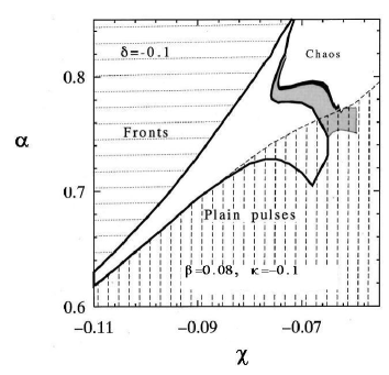
Figure 1: (a) Regions of existence of various solutions obtained from numerical simulations [3] of the complex GL equation (1) without NM. The parameters are $\delta=-0.1,\ \kappa=-0.1$ and $\beta=0.08,$ (b) Regions of existence and stability of FPs with NM. The parameters of NM are: $f=10$ and $\omega=63$.

In the Fig. 1a, regions of the existences of the different types of solutions of Eq. (2) and the corresponding boundaries are presented. Fig. 1a, taken from work [3], shows in plane $(\chi,\alpha)$ results of numerical simulations of the original complex GL equation (2) for values of parameters $\delta=-0.1$, $\kappa=-0.1$, $\beta=0.08$ and $f=0$. The region with vertical shading corresponds to stationary solitons. Solutions describing fronts exist in the region with horizontal shading. The central region between these two regions corresponds to the pulsating solitons with the single-period variation. A small grey area corresponds to multi-period pulsating solitons. An white area in the upper right corner denotes region of chaotic solitons. Stationary and pulsating solitons of Eq. (2) with $f=0$ correspond to stable FPs and LCs in dynamical model ((9)-(11) with $f=0$)(see e.g. [6]).

Stable FPs of Eqs (9)-(11) correspond to solitons with oscillating parameters are in Eq (2). Oscillations of the parameters are due to NM. Stable LCs of Eqs (9)-(11) might also manifest themselves as oscillating solitons in Eq (2). We do not distinguish between these two types, and all solitons with almost periodic variations of the parameters are referred as managed oscillating (MO) solitons.

Figure 2a shows the evolution of the soliton amplitude without and with NM. We see that a stationary soliton is transforming to a MO soliton under the action of NM. Figure 2b shows the corresponding evolution of the field.

We obtain an analogue of Fig. 1a for the case, when NM is applied, with the NM strength is $\sigma^{2}=0.013$ (or $f=10$ and $\omega=63$). The results obtained are displayed in Fig. 1b, where for comparison with Fig. 1a, the central region is copied.

The dash-dotted line and the dashed line are obtained from Eqs. (9)-(11). The dash-dotted line is the area boundary, below which FPs are stable in absence of NM. Under the action of NM, this boundary is shifted down into a position which is marked by the dashed line. The dotted line, obtained by numerical simulations of the complex GL equation (2) with NM, represents the upper boundary of MO solitons. It is seen, that the agreement between the VA system (9) - (11) and Eq. (2) is good. The region above the dotted line corresponds to irregular solutions (fronts, chaotic solutions and others).

Figure 2: (a) The pulse amplitude evolution without (line 1) and with (line 2) NM.  (b) Evolution of the MO soliton. The parameters are $\delta=-0.1,\ \kappa=-0.1,\ \beta=0.08,\ \chi=-0.08\ \alpha=0.61,\ f=10$ and $\omega=65$.

Numerical simulations of Eq (2) show that the strong management regime ($\sigma^{2}\sim O(1)$) is effective for stabilization of exploding solitons solutions, transforming them into oscillating solitons. In Fig. 3(a) the evolution of an ES in the absence of NM is presented. The evolution of solutions under NM at the same values of parameters and for $f=10$ and $\omega=10$ is displayed in Fig. 3(b). It is seen that the ES is transformed into a oscillating solution.

Figure 3: (a) An exploding soliton without NM. The parameters are $\delta=-0.1,\ \kappa=-0.1,\ \beta=0.125,\ \chi=-0.6$ ,  $\alpha=1.0$. (b) An oscillating solution for the same values parameters and with NM ($f=10$  and  $\omega=10$).

In Fig. 4(a), taken from work [3], the region of existence of ESs in the $(\chi,\alpha$) plane is shown. The upper white region corresponds to stationary solitons, while the lower white region corresponds to decaying solutions. The middle grey region is a region of ES solutions. We find by direct numerical simulations of Eq. (2) for $f=10$ and $\omega=10$ (see Fig. 4b) that under NM these regions are deformed. As can be seen, the region of the ES existence is strongly reduced. Nonlinearity management leads to the suppression of ESs, transforming them into oscillating solutions (i.e. enlarging the upper white area), or into decaying solutions (enlarging lower white area). Also, under the action of NM a part of stationary solutions transforms into irregular solutions (fronts, chaotic solutions and others), see the black area in Fig. 4b). Thus we conclude that ESs are effectively suppressed under the action of NM.

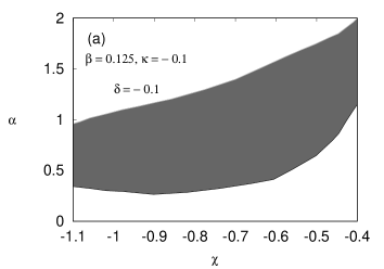
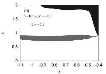
Figure 4: (a) A region in $(\alpha,\chi)$ plane different types of the the dynamics, found exist [3], in the absence NM. The middle grey area corresponds to ESs. (b) Same region when there is of NM with $f=10$  and  $\omega=10$.

5 Conclusion.

In conclusion, we have investigated the complex GL equation with the strong nonlinearity management. The averaged complex GL equation has been derived. We show the existence of nonlinearity managed dissipative solitons. We employ the variational approach to this averaged equation and derive the system of equations for dissipative soliton parameters. Numerical simulations show that the explosion regime in the evolution of the dissipative soliton is suppressed by this scheme. The region of parameters, where explosions are suppressed, has been obtained. This type of suppression can be observed in experiments that involve fiber-ring lasers with the nonlinearity management.

6 Acknowledgments

We thank Dr. E. N. Tsoy for fruitful discussions. The work was supposed by the grant FA-F2-004 of Ministry of Innovative Development of the Republic of Uzbekistan.

References

- [1] N. Akhmediev, A. Ankiewicz (Eds.), Dissipative Solitons, Springer, Berlin, Germany (2008)
- [2] P. Grelu, N. Akhmediev, Nat. Photonics 6 (2012) 84.
- [3] N. Akhmediev, J.M. Soto-Crespo, G. Town, Phys. E, Rev. 63 (2001) 056602.
- [4] R. J. Deissler H. R. Brand, Phys. Rev. Lett. 72 (1994) 478.
- [5] J. M. Soto-Crespo, M. Grapinet, Ph. Grelu, N. Akmediev, Phys.Rev. E 70 (2004) 066612.
- [6] E. N. Tsoy, N. A. Akhmediev, Phys.Lett. A 343 (2005) 417.
- [7] S. T. Cundiff, J. M. Soto-Crespo, N. Akhmediev, Phys.Rev.Lett. 88 (2002) 073903.
- [8] A. F. Runge, N. G. Broderick, M. Erkintalo, Optica 2 (2015) 36.
- [9] Z. W. Wei et al. Opt. Lett. 45 (2019) 382459.
- [10] S. V. Gurevich, S. Schelte, J. Javaloyes, Phys. Rev. A 99 (2019) 061803.
- [11] S. C. V. Lutas, M. F. S. Fereira, Opt. Lett. 35 (2010) 1771.
- [12] J. M. Soto-Crespo, N. Akhmediev, and A. Ankiewicz, Phys.Rev.Lett. 85 (2000) 2937.
- [13] Optics Express J. Fatome, S. Pitois, P. Tchofo Dinda, and G. Millot, Optics Express 11 (2003) 1553-1558
- [14] M. J. Ablowitz, T. P. Horkis, B. Ilan, Phys. Rev. A 77 (2008) 33814.
- [15] G. Biondini, Nonlinearity 21 (2008) 2849.
- [16] S. K. Turitsyn, B. J. Bale, M. Fedoryuk, Phys.Rep. 521 (2012) 135.
- [17] A. Biswas, D. Milovic, M. Edvards, Mathematical Therory of dispersion - managed optical solitons. Springer - Verlag, Heydelberg, 2010
- [18] F. O. Ilday, F. W. Wise, JOSA B 19 (2002) 470.
- [19] L. Berge, P. L. Christiansen, Yu. B. Gaididei, V. K. Mezentsev, J. J. Rasmussen, Opt. Lett. 25 (2000) 1037.
- [20] I. Towers, B. A. Malomed, JOSA B 22 (2005) 2200.
- [21] F. Kh. Abdullaev, R. A. Kraenkel, Phys. Lett. A 272 (2001) 395.
- [22] F. Kh. Abdullaev, J. G. Caputo. B. A. Malomed, R. A. Kraenkel, Phys. Rev A 67 (2003) 013605.
- [23] H. Saito, M. Ueda, Phys. Rev. Lett. 90 (2003) 040403.
- [24] G. D. Montesinos, V. M. Perez-Garcia, H. Michinel, Phys. Rev. Lett. 92 (2004) 133901.
- [25] E. P. Ippen, Appl. Phys. B 58 (1994) 159.
- [26] Z. Bakonyi, D. Michaelis, U. Peschel, G. Onishchukov, F. Lederer, J. Opt. Soc. Am., 19 (2002) 47.
- [27] S. Beheshti, K. Law, P. G. Kevrekidis, M. Porter, Phys.Rev. A 78 (2008) 025805.
- [28] D. E. Pelinovsky, P. G. Kevrekidis, D. J. Frantzeskakis, Phys.Rev. E 70 (2004) 047604.
- [29] F. Kh. Abdullaev, E. N. Tsoy, B. A. Malomed, R. A. Kraenkel, Phys. Rev. A 68 (2003) 053606.
- [30] F.Kh. Abdullaev, A. A. Abdumalikov, and R. M. Galimzyanov, Physica D 238 (2009) 1345.
- [31] D. Anderson, Phys. Rev. A (1983) 3135
- [32] S. N. Vlasov, V. A. Petrishev, V. I. Talanov, Radiofizika 14 (1975) 1353, (In Russian).
- [33] V. Filho, F. Kh. Abdulllaev, A. Gammal, L. Tomio, Phys.Rev. A 63 (2001) 053603
- [34] Y. Du, X. Shu, Opt. Express 26 (2018) 5564.
- [35] J. Peng, H. Zeng, Communications Physics 2 (2019) 34.
- [36] C. Cartes, O. Descalzi, Fibers and Integ. Optics 34 (2015) 14.