On the Darwin–Howie–Whelan equations for
the scattering of fast electrons described by
the Schrödinger equation

Abstract

The Darwin–Howie–Whelan equations are commonly used to describe and simulate the scattering of fast electrons in transmission electron microscopy. They are a system of infinitely many envelope functions, derived from the Schrödinger equation. However, for the simulation of images only a finite set of envelope functions is used, leading to a system of ordinary differential equations in thickness direction of the specimen. We study the mathematical structure of this system and provide error estimates to evaluate the accuracy of special approximations, like the two-beam and the systematic-row approximation.

35J10, 74J20

1 Introduction

The Darwin–Howie–Whelan (DHW) equations, which are often simply called Howie–Whelan equations (cf. [7, Sec. 2.3.2] or [10, Sec. 6.3]), are widely used for the numerical simulation of transmission-electron microscopy (TEM) images, e.g. see [15] for the software package pyTEM or [19, 26] for the software CUFOUR. They describe the propagation of electron beams through crystals and can be applied to semiconductor nanostructures, see [3, 17, 13, 14]. They provide a theoretical basis that allows one to construct suitable experimental set ups for obtaining microscopy data on the one hand, and can be used to analyze measured data in more details on the other hand. The origins of this model go back to Darwin in [2] with major generalizations by Howie and Whelan in [6]. Moreover, the DHW equations are closely related to the approach based on the Bethe potentials used in [23].

Currently, many quantitative methods emerge for applications in TEM [15, 26], holography [12, 8], scanning electron microscopy [18, 16], electron backscatter diffraction [25, 27], and electron channelling contrast imaging [17], where quantitative evaluations of micrographs are compared to simulation results to replace former qualitative observations by rigorous measurements of embedded structures in crystals. For that reason it is essential to evaluate the accuracy and the validity regime of the chosen modeling schemes and simulation tools. In electron microscopy this includes the heuristic approaches to select the relevant beams in multi-beam approaches [25, 15, 26]. The present work is devoted to the theory behind the DHW equations and thus provides mathematical arguments and refinements for the beam-selection problem.

The DHW equations can be derived from the time-dependent Schrödinger equation for the wave function $\psi(t,x)$ of the electrons:

(1) $$\mathrm{i}\hbar\,\frac{\partial\psi(t,x)}{\partial t}=-\frac{\hbar^{2}}{2m}\,\Delta\psi(t,x)-qV_{\mathrm{C}}(x)\psi(t,x),$$

such that $|\psi(t,x)|^{2}$ denotes the probability density of the electrons. Here $x$ denotes the position in the specimen, $V_{\mathrm{C}}$ is a periodic potential describing the electronic properties of the crystal, $m=m_{0}\gamma$, with $\gamma$ the relativistic mass ratio and $m_{0}$ the electron rest mass, $\hbar$ Planck’s constant and $q$ the elementary charge. Using $\psi(t,x)=\mathrm{e}^{-\mathrm{i}4\pi^{2}\frac{\hbar}{2m}|k_{0}|^{2}t}\Psi(x)$ we obtain the static Schrödinger equation

(2) $$\Delta\Psi(x)+(2\pi|k_{0}|)^{2}\Psi(x)=-4\pi^{2}{\mathcal{U}}(x)\Psi(x),$$

where $k_{0}$ is the wave vector of the incoming beam and ${\mathcal{U}}$ is the reduced electrostatic potential defined as ${\mathcal{U}}(x)=\frac{2mq}{\hbar^{2}}V_{\mathrm{C}}(x)$. The periodicity lattice of the crystal and its potential ${\mathcal{U}}$ is denoted by $\Lambda$ and its dual lattice by $\Lambda^{*}$.

We decompose the spatial variable $x$ into the transversal part $y$ orthogonal to the thickness variable $z\in[0,z_{*}]$, where $z=0$ is the side where the monochromatic electron beam $\psi(t,x)=\mathrm{e}^{\mathrm{i}(-4\pi^{2}\frac{\hbar}{2m}|k_{0}|^{2}t+2\pi k_{0}\cdot x)}$ with wave vector $k_{0}$ enters, and $z=z_{*}$ is the side where the scattered beam exits the specimen, see Figure 1.

  Figure 1: The incoming wave with wave vector $k_{0}$ enters the specimen, is partially transmitted, and generates waves with nearby wave vectors $k_{0}{+}g$.

The so-called “column approximation” restricts the focus to solutions of (2) that are exactly periodic in $y$ and are slow modulations in $z$ of a periodic profile in $z$. Hence, we seek solutions in the form

(3) $$\Psi(x)=\sum_{g\in\Lambda^{*}}\psi_{g}(z)\,\mathrm{e}^{\mathrm{i}\,2\pi k_{0}\cdot x}\,\mathrm{e}^{\mathrm{i}\,2\pi g\cdot x},$$

where $\Lambda^{*}\subset{\mathbb{R}}^{d}$ denotes the dual lattice and $\psi_{g}$ is the slowly varying envelope function of the beams in the directions of the wave vector $g\in\Lambda^{*}$. Note that now $g=0$ corresponds to the main incoming beam. Inserting (3) into (2) and dropping the term $\frac{{\mathrm{d}}^{2}}{{\mathrm{d}}z^{2}}\psi_{g}$ one obtains the DHW equations for infinitely many beams (see Section 2 for more details on the modeling):

(4) $$\frac{\rho_{g}}{\pi}\,\frac{{\mathrm{d}}}{{\mathrm{d}}z}\psi_{g}(z)=\mathrm{i}\Big{(}\sigma_{g}\psi_{g}(z)+\sum_{h\in\Lambda^{*}}U_{g-h}\psi_{h}(z)\Big{)},\quad\psi_{g}(0)=\delta_{0,g},\quad\text{for }g\in\Lambda^{*}$$

$$\text{where }\ \rho_{g}=(k_{0}{+}g)\cdot\nu\ \text{ and }\ \sigma_{g}=|k_{0}|^{2}-|k_{0}{+}g|^{2},$$

where $\nu=(0,...,0,1)^{\top}$ is the normal to the crystal surface and where $U_{g}$ are the Fourier coefficients of the periodic potential ${\mathcal{U}}$, i.e. ${\mathcal{U}}(x)=\sum_{g\in\Lambda^{*}}U_{g}\mathrm{e}^{\mathrm{i}2\pi g\cdot x}$.

In fact, to make (4) equivalent to the full static Schrödinger equation (2) one has to add the second derivatives with respect to $z$, namely $\frac{1}{4\pi^{2}}\frac{{\mathrm{d}}^{2}}{{\mathrm{d}}z^{2}}\psi_{g}(z)$. Dropping these terms constitutes the DHW equations, which are solved as an initial-value problem with the simple initial condition $\psi_{g}(0)=\delta_{0,g}$ (Kronecker symbol) for the incoming beam, and $\big{(}\psi_{g}(z_{*})\big{)}_{g\in\Lambda^{*}}$ describes all exiting beams. In contrast, the full second-order equations would need a careful setup of transmission and reflection conditions at $z=0$ and $z=z_{*}$, and then are able to account for the backscattering of electrons. We refer to [21] and our Remark 2.1 for the justification of this approximation for electrons with high energy that are typical for TEM.

Most often, the DHW equations are stated in the form that the equation for $\psi_{g}$ is divided by $\rho_{g}/\pi$, and then it features the important excitation error $s_{g}:=\sigma_{g}/(2\rho_{g})$. However, the mathematical structure can be seen better in the form (4): the right-hand side is given by the imaginary unit $\mathrm{i}$ multiplied by a Hermitian operator under our standard assumption that ${\mathcal{U}}$ is a real potential, i.e. $U_{-g}=\overline{U}_{g}$. This will be crucial for the subsequent analysis based on the associated Hamiltonian structure.

In the physical literature, the DHW equations are formally stated as a system for infinitely many beam amplitudes $\psi_{g}$ with $g$ running through the whole dual lattice $\Lambda^{*}$. For the numerical solution one has to select a finite set ${\mathbf{G}}\subset\Lambda^{*}$ of relevant beams, e.g. the classical two-beam approximation, see Section 4.3. To our knowledge there is no systematic discussion about the accuracy of approximations depending on the choice of ${\mathbf{G}}$. The main goal of this paper is to provide mathematical guidelines for optimal choices that are justified by exact error estimates.

First, we observe that (4) for all $g\in\Lambda^{*}$ is probably ill-posed, in particular, because of $\rho_{g}$ changing sign and, even worse, becoming $0$ or arbitrarily close to $0$. It is clear that neglecting the term $\frac{1}{4\pi^{2}}\frac{{\mathrm{d}}^{2}}{{\mathrm{d}}z^{2}}\psi_{g}(z)$ cannot be justified for such $g$’s. Hence, one should realize that the DHW equations (4) is only useful for $g$ where $\rho_{g}$ is close to $\rho_{0}=k_{0}\cdot\nu>0$, see Section 2.2. But the main questions of beam selection remain:
•  What does “close” mean?
•  How many and which beams are needed to obtain a reliable approximation for the
• solution of the Schrödinger equation, in particular for high-energy electron beams?

We approach these questions by systematically investigating the dependence of the solutions ${\bm{\psi}}^{\mathbf{G}}=(\psi_{g})_{g\in{\mathbf{G}}}$ on the chosen subset ${\mathbf{G}}$ of the dual lattice $\Lambda^{*}$ for which we solve (4). More precisely, for ${\mathbf{G}}\subset\Lambda^{*}$ we define DHW_G to be the set of equations

(5) $$\frac{\rho_{g}}{\pi}\,\frac{{\mathrm{d}}}{{\mathrm{d}}z}\psi_{g}(z)=\mathrm{i}\Big{(}\sigma_{g}\psi_{g}(z)+\sum_{h\in{\mathbf{G}}}U_{g-h}\psi_{h}(z)\Big{)},\quad\psi_{g}(0)=\delta_{0,g},\quad g\in{\mathbf{G}}.$$

We will shortly write this in vector-matrix form

(6) $$R\overset{\text{\LARGE.}}{{\bm{\psi}}}(z)=\mathrm{i}\big{(}\Sigma{+}{\mathbb{U}}\big{)}\,{\bm{\psi}}(z),\quad{\bm{\psi}}(0)=(\delta_{0,g})_{g\in\Lambda^{*}},\quad{\bm{\psi}}=(\psi_{g})_{g\in{\mathbf{G}}}.$$

For $\gamma\in{]0,1[}$ and $M>0$, we define two important classes of admissible beam sets by

$${\mathbf{G}}_{\gamma}:=\big{\{}\,g\in\Lambda^{*}\>\big{|}\>\rho_{g}\geq\gamma\rho_{0}\,\big{\}}\quad\text{and}\quad{\mathbf{G}}^{M}:=\big{\{}\,g\in\Lambda^{*}\>\big{|}\>|g|\leq M\,\big{\}},$$

such that always $0\in{\mathbf{G}}^{M}\cap{\mathbf{G}}_{\gamma}$ and $\rho_{g}>0$ for $g\in{\mathbf{G}}_{\gamma}$. Throughout we will only consider the case of such $M>0$ that ${\mathbf{G}}^{M}\subset{\mathbf{G}}_{\gamma}$ for some $\gamma>0$.

We first show in Proposition 3.1 that for each ${\mathbf{G}}\subset{\mathbf{G}}_{\gamma}$ the system DHW_G has a unique solution ${\bm{\psi}}^{\mathbf{G}}:{\mathbb{R}}\to\mathfrak{H}({\mathbf{G}})$, where $\mathfrak{H}({\mathbf{G}})$ is the Hilbert space generated by the scalar product

$$\big{\langle}{\bm{\psi}},{\bm{\varphi}}\big{\rangle}_{\mathbf{G}}:=\sum_{g\in{\mathbf{G}}}\rho_{g}\psi_{g}\overline{\bm{\varphi}}_{g}\quad\text{and the norm }\|{\bm{\psi}}\|_{\mathbf{G}}:=\big{\langle}{\bm{\psi}},{\bm{\psi}}\big{\rangle}_{\mathbf{G}}^{1/2}.$$

In Section 3.3 we will show that the influence of the exact choice of the set ${\mathbf{G}}$ is not important if we stay inside ${\mathbf{G}}_{\gamma}$ and if we have enough modes around $g=0$. More precisely, for two sets ${\mathbf{G}}^{(1)}$ and ${\mathbf{G}}^{(2)}$ satisfying ${\mathbf{G}}^{M}\subset{\mathbf{G}}^{(j)}\subset{\mathbf{G}}_{\gamma}$ the unique solutions ${\bm{\psi}}^{(j)}$ can be compared on ${\mathbf{G}}^{M}$ as follows:

(7) $$\big{\|}{\bm{\psi}}^{(1)}(z)|_{{\mathbf{G}}^{M}}-{\bm{\psi}}^{(2)}(z)|_{{\mathbf{G}}^{M}}\big{\|}_{{\mathbf{G}}^{M}}\leq\widehat{C}_{\mathcal{U}}\>\mathrm{e}^{\widehat{\kappa}|z|-\widehat{\alpha}M}\,\|{\bm{\psi}}(0)\|_{\mathbf{G}}\quad\text{for all }z\in{\mathbb{R}}\,.$$

The coefficients $\widehat{\kappa}$ and $\widehat{\alpha}$ can also be given explicitly, see Corollary 3.11. For this estimate, we use the fundamental assumption that the Fourier coefficients $U_{g}$ of the scattering potential ${\mathcal{U}}$ decay exponentially:

(8) $$|U_{g}|\leq C_{\mathbb{U}}\,\mathrm{e}^{-\alpha_{\mathbb{U}}|g|}\quad\text{for all }g\in\Lambda^{*}.$$

Hence, we see that scattering allows the energy to travel from the transmitted beam $g=0$ to the diffracted beams linearly with respect to the distance $|z|$. Note that we interpret equation (6) as an autonomous Hamiltonian system, such that estimates like (7) hold for all $z\in{\mathbb{R}}$. However, to evaluate realistic errors for a specimen we restrict to $z\in[0,z_{*}]$, see e.g. (9). In particular, (7) provides a good bound on $[0,z_{*}]$ as long as $z_{*}$ is much smaller than $\widehat{\alpha}M/\widehat{\kappa}$.

In a second step we are able to reduce the set ${\mathbf{G}}$ even further by restricting $g$ into a neighborhood of the Ewald sphere

$${\mathbb{S}}_{\mathrm{Ew}}:=\big{\{}\,g\in{\mathbb{R}}^{d}\>\>\big{|}\>\>|k_{0}|^{2}-|k_{0}{+}g|^{2}=0\,\big{\}}.$$

Indeed, in TEM the incoming beam with wave vector $k_{0}$ is chosen exactly in such a way that the intersection of the Ewald sphere ${\mathbb{S}}_{\mathrm{Ew}}$ with the dual lattice $\Lambda^{*}$ contains, in addition to the transmitted beam $g=0$, a special number of other points.

From the energetic point of view it is important to observe that the modulus $|s_{g}|=|\sigma_{g}|/(2\rho_{g})$ of the excitation errors for wave vectors $g$ not close to the Ewald sphere are much bigger than $|U_{g}|/\rho_{g}$. To exploit this, we use the classical norm and energy conservation for the linear Hamiltonian system (6), namely $\|{\bm{\psi}}(z)\|_{\mathbf{G}}=\|{\bm{\psi}}(0)\|_{\mathbf{G}}$ and $\|R^{-1}(\Sigma{+}{\mathbb{U}}){\bm{\psi}}(z)\|_{{\mathbf{G}}}=\|R^{-1}(\Sigma{+}{\mathbb{U}}){\bm{\psi}}(0)\|_{{\mathbf{G}}}$ together with the estimate

$$\|R^{-1}\Sigma{\bm{\psi}}(z)\|^{2}_{{\mathbf{G}}}\leq 2\|R^{-1}(\Sigma{+}{\mathbb{U}}){\bm{\psi}}(z)\|^{2}_{{\mathbf{G}}}+2\|R^{-1}{\mathbb{U}}{\bm{\psi}}(z)\|^{2}_{{\mathbf{G}}}.$$

Since $\|R^{-1}(\Sigma{+}{\mathbb{U}}){\bm{\psi}}(0)\|_{{\mathbf{G}}}$ is controlled by the initial value ${\bm{\psi}}(0)={\bm{\delta}}=(\delta_{0,g})$ and $\|R^{-1}{\mathbb{U}}{\bm{\psi}}(z)\|^{2}_{{\mathbf{G}}}\leq{\widehat{c}_{\mathbb{U}}}\|{\bm{\psi}}(z)\|^{2}_{{\mathbf{G}}}$, we obtain a good bound on $\sum_{g\in{\mathbf{G}}}\rho_{g}|s_{g}\psi_{g}(z)|^{2}$ in terms of the initial data. This allows us to quantify the smallness of the amplitudes $|\psi_{g}(z)|$ if the excitation error $|s_{g}|$ lies above a cut-off value $\widetilde{s}_{*}$, see Section 3.4.

With this, we provide an error bound for the so-called Laue-zone approximation ${\bm{\psi}}^{\mathrm{LOLZ}}$ (cf. Section 4.2), where we choose $M\sim|k_{0}|^{1/2}$ to approximate a spherical cap of the Ewald sphere, which has the height of one dual lattice spacing. For the cut-off $\widetilde{s}_{*}$ one can choose a constant that is proportional to the spacing of the dual lattice. The final error bound compares the solutions ${\bm{\psi}}^{\gamma}$ and ${\bm{\psi}}^{\mathrm{LOLZ}}$ of DHW${}_{{\mathbf{G}}_{\gamma}}$ and DHW${}_{{\mathbf{G}}_{\mathrm{LOLZ}}}$, respectively, on the interval $z\in[0,z_{*}]$:

(9) $$\|{\bm{\psi}}^{\mathrm{LOLZ}}(z)-{\bm{\psi}}^{\gamma}(z)|_{{\mathbf{G}}_{\mathrm{LOLZ}}}\|_{{\mathbf{G}}_{\mathrm{LOLZ}}}\leq N_{1}\Big{(}\frac{1}{|\alpha_{*}k_{0}|^{2}}+\frac{\alpha_{*}C_{\mathbb{U}}^{2}}{|k_{0}|^{2}}\,z_{*}\Big{)}\|{\bm{\delta}}\|_{\mathbf{G}}\,.$$

Here $N_{1}$ is a computable, dimensionless constant, and $\alpha_{*}$ is the lattice constant of $\Lambda$. The first error term arises from the restriction of ${\mathbf{G}}_{\gamma}$ to ${\mathbf{G}}^{M}$, and it is small for high energies, i.e. $|\alpha_{*}k_{0}|\gg 1$. The second error term arises from the restriction to the neighborhood of the Ewald sphere and has the form

$$\frac{\alpha_{*}}{\ell_{\mathrm{scatt}}}\>\frac{z_{*}}{\ell_{\mathrm{scatt}}}\qquad\text{with global scattering length }\ell_{\mathrm{scatt}}=\frac{|k_{0}|}{C_{\mathbb{U}}}.$$

Since we always have $z_{*}\approx\ell_{\mathrm{scatt}}$ we see that the error is small if the scattering length $\ell_{\mathrm{scatt}}$ is much bigger than the lattice constant $\alpha_{*}$, which is indeed the case in TEM experiments with specimens of about 100 atomic layer thickness.

A similar error analysis is then done for the two-beam approximation and the systematic-row approximation, see Sections 4.3 and 4.4. Finally, Section 5 presents numerical simulations that underpin the quality of the error bounds and thus provide a justification of the numerics done when solving the DHW equations as in [15].

The authors are not aware of any mathematical analysis for beam-like, high-energy solutions of the static Schrödinger equation. There is a large body of works on the semiclassical limit of the time-dependent Schrödinger equation $\mathrm{i}\varepsilon\partial_{t}\psi=-\varepsilon^{2}\Delta\psi+V(\frac{1}{\varepsilon}x)\psi$ with a periodic potential (cf. [5, 1, 9]) that are related in spirit. There, $|k|$ is of order $1/\varepsilon\gg 1$ such that $\varepsilon|k|\approx 1$ is a different regime as our case $\alpha_{*}|k_{0}|\gg 1$. Moreover, there initial-value problem for the time-dependent Schrödinger equations are studied assuming smooth envelope functions, while we are concerned with static scattering-type solutions of a Helmholtz-type Schrödinger equation.

We close this introduction with some remarks concerning the usage of the DHW equations in TEM imaging of objects embedded in crystals, such as quantum dots. There, the crystal structure changes slightly because of the different properties of the embedded materials. In the simplest case one assumes that the crystal lattice stays intact, but the potential ${\mathcal{U}}$ is no longer exactly periodic but varies on a larger length scale. Nevertheless one can assume that electron beams can propagate vertically through the crystal, i.e. the column approximation holds. As the embedded material has different chemical composition the potential remains locally periodic, but on a mesoscale depends on the thickness variable $z\in[0,z_{*}]$ as well as the horizontal variables $y_{1}$ and $y_{2}$. Using the column approximation the latter variables are considered as parameters that are used for scanning the probe pixel by pixel. The associated DHW equations then take the form

$$R\frac{{\mathrm{d}}}{{\mathrm{d}}z}{\bm{\psi}}=\mathrm{i}\big{(}\Sigma+{\mathbb{U}}(y_{1},y_{2},z)\big{)}{\bm{\psi}},\quad{\bm{\psi}}(0)={\bm{\delta}}.$$

Typically, the objective aperture of the microscope selects only a single beam ${\widehat{g}}\neq 0$ (e.g. $g=(0,4,0)$ in [14]), and its exit intensity

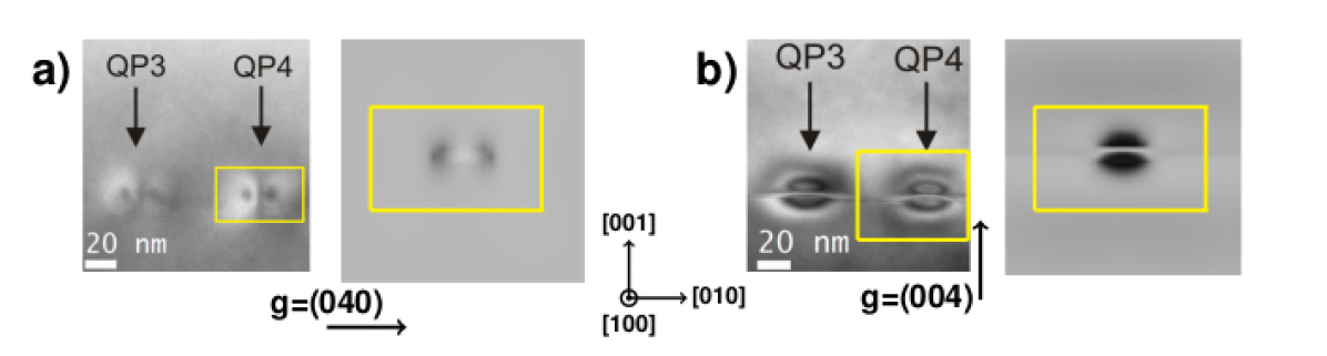
Figure 2: TEM images of lens-shaped InAs quantum dots embedded in a GaAs matrix: (a) Experimental dark field of (040) beam and the corresponding image from a DHW simulation. (b) Experimental dark field of (004) beam and the corresponding image from a DHW simulation. Yellow areas indicate the same areas in experimental and simulated images. Adapted by permission from Springer Nature: Optical and Quantum Electronics, [14, Fig. 6], $\copyright$ 2020.

$I_{\widehat{g}}(y_{1},y_{2}):=|\psi_{\widehat{g}}(z_{*};y_{1},y_{2})|^{2}$ is recorded in dependence of the horizontal position $(y_{1},y_{2})$. The analysis of the $(y_{1},y_{2})$-dependence goes beyond of this work and will be addressed in future research. In general, the term “bright-field image” is used, when the undiffracted beam related to ${\widehat{g}}=0$ is included in the aperture. The term “dark-field” is used for images, where only one diffracted beam ${\widehat{g}}\neq 0$ forms the image. In Figure 2 we see two dark-field TEM images of InAs quantum dots, for the $(040)$ beam and the $(004)$ beam, and the corresponding simulated images, all taken from [14].

The methods developed here for the DHW equations address more generally the question of beam selection for electron waves in crystals, which is also important for calculations based on the Bloch wave expansion [23] or electron backscatter diffraction [25]. In particular, our methods provide mathematical error estimates that allow us to understand and refine beam selection scheme in situations where the classical two-beam approach is not sufficient, see [22, 13, 26, 14]. The problem of beam selection will be even more important because of the recent trend to use lower acceleration voltages, see e.g. [16, 17], where $|k_{0}|$ is smaller and scattering into more beams occurs naturally. This is also why we try to make all estimates as explicit as possible in their dependence on the data such as $|k_{0}|$, $C_{\mathbb{U}}$, and $\alpha_{\mathbb{U}}$ (cf. (8)).

2 The modeling

2.1 Derivation of the DHW equations

Transmission electron microscopy uses high-energy electron beams, which can be described by the relativistic wave equation for an electron in an electrostatic field, see [3]:

(10) $$\Delta\Psi(x)+(2\pi|k_{0}|)^{2}\Psi(x)=-4\pi^{2}{\mathcal{U}}(x)\Psi(x),$$

where $k_{0}$ is the wave vector of the incoming beam, and ${\mathcal{U}}$ is the reduced electrostatic potential. The modulus of the wave vector is related to the (relativistic) wave length by $|k_{0}|=1/\lambda_{0}$. The wave length $\lambda_{0}$ is obtained from the acceleration voltage $E$ via

$$\lambda_{0}=\hbar\big{/}{\sqrt{2m_{0}qE\big{(}1{+}\tfrac{qE}{2m_{0}c_{0}^{2}}\big{)}}},$$

where $\hbar$ is the Planck’s constant, $m_{0}$ is the electron rest mass, $q$ is the elementary charge, and $c_{0}$ is the speed of light. The reduced electrostatic potential is given by

(11) $${\mathcal{U}}(x)=\frac{2m_{0}q}{\hbar^{2}}\,\gamma\,V_{\mathrm{C}}(x)\quad\text{with the relativistic mass ratio }\gamma=1+\frac{qE}{m_{0}c_{0}^{2}}\,.$$

Here $V_{\mathrm{C}}$ is the (possibly complex) electrostatic potential such that the reduced potential ${\mathcal{U}}$ has the unit $\mathrm{m}^{-2}$. The table in Figure 3 shows typical values for the wave vector $k_{0}$ and the mass ratio $\gamma$ for different values of the acceleration voltage $E$.

$E$ $k_{0}$ $\gamma$ $\beta=v/c_{0}$ 100 270.165 1.196 0.548 200 398.734 1.391 0.695 300 507.937 1.587 0.777 400 608.293 1.783 0.828    Figure 3:   Acceleration voltage $E$ in $\mathrm{kV}$, wave number $k_{0}$ in $\mathrm{nm^{-1}}$, mass ratio $\gamma$, and relative velocity $\beta=v/c_{0}$. (Table adapted from [3, p. 93 Table 2.2])

The periodicity of the potential ${\mathcal{U}}$ is given by the (primal) lattice $\Lambda\subset{\mathbb{R}}^{d}$ via ${\mathcal{U}}(x{+}r)={\mathcal{U}}(x)$ for all $x\in{\mathbb{R}}^{d}$ and all lattice vectors $r\in\Lambda$. The dual lattice is

$$\Lambda^{*}:=\big{\{}\,g\in{\mathbb{R}}^{d}\>\big{|}\>g\cdot r\in{\mathbb{Z}}\text{ for all }r\in\Lambda\,\big{\}}.$$

With this, we are able to write ${\mathcal{U}}$ by its Fourier expansion ${\mathcal{U}}(x)=\sum_{g\in\Lambda^{*}}\mathrm{e}^{\mathrm{i}\,2\pi g\cdot x}\>U_{g}.$

The solution $\Psi$ of the Schrödinger equation is assumed to have an envelope form given by a plane wave $\mathrm{e}^{\mathrm{i}\,2\pi k_{0}\cdot x}$ times a slowly varying function $\widetilde{\Psi}$, where $k_{0}$ is the wave vector for the incoming electron beam. Throughout the paper, we decompose $x\in{\mathbb{R}}^{d}$ into a in-plane component $y\in{\mathbb{R}}^{d-1}$ and a transversal component $z\in{\mathbb{R}}$, i.e. after rotating the coordinate axis we have $x=(y,z)$. To comply with physicists convention, the $z$ direction is orientated roughly parallel to the electron beam, while the outwards normal to the specimen at the exit plane $z=z_{*}$ denoted by ${\bm{\nu}}$, is assumed to be

$${\bm{\nu}}:=(0,\ldots,0,1)^{\top}.$$

We emphasize that the lattices $\Lambda$ and $\Lambda^{*}$ are not necessarily aligned with one of the directions ${\bm{\nu}}$ or $k_{0}$, but we always assume $k_{0}\cdot{\bm{\nu}}>0$, see Figure 1.

In accordance with the experimental setup of TEM we are looking for solutions that are slow modulations in the transversal direction $z$ of a periodic Bloch-type function $\widetilde{\Psi}=\sum_{g\in\Lambda^{*}}\psi_{g}\mathrm{e}^{2\pi\mathrm{i}g\cdot x}$ times the carrier wave $\mathrm{e}^{\mathrm{i}\,2\pi k_{0}\cdot x}$ (multi-beam approach). More precisely, we seek solutions in the form

(12) $$\Psi(x)=\Psi(y,z)=\sum_{g\in\Lambda^{*}}\psi_{g}(z)\,\mathrm{e}^{\mathrm{i}\,2\pi k_{0}\cdot x}\,\mathrm{e}^{\mathrm{i}\,2\pi g\cdot x},\quad\text{where }x=(y,z).$$

From a physics point of view, this multi-beam ansatz represents the diffraction of the incoming beam $\psi_{0}$ in different discrete directions $g$, given by the dual lattice. The use of an objective aperture in TEM allows for restricting the set of transmitted beams forming the image in the microscope. Bright field and dark field imaging allows us to access the specific components $\psi_{g}$ of the multi-beam ansatz.

Using the Fourier expansion of ${\mathcal{U}}$ we see that $\Psi$ given in (12) solves the Schrödinger equation (10) if and only if the following system of ODEs is satisfied:

(13) $$\partial_{z}^{2}\psi_{g}(z)+\mathrm{i}\;\!4\pi\;\!\rho_{g}\partial_{z}\psi_{g}(z)+4\pi^{2}\sigma_{g}\psi_{g}(z)=-4\pi^{2}\sum_{h\in\Lambda^{*}}U_{g-h}\psi_{h}(z)\quad\text{for }g\in\Lambda^{*},$$

$$\text{where }\rho_{g}:=(k_{0}{+}g)\cdot{\bm{\nu}}\ \text{ and }\sigma_{g}:=|k_{0}|^{2}-|k_{0}{+}g|^{2}=-|g|^{2}{-}2k_{0}\cdot g.$$

Recalling ${\bm{\nu}}=(0,..,1)^{\top}$, we see that $\rho_{g}$ is positive for $g\approx 0$, while $\sigma_{g}$ changes sign in balls around $g=0$.

Next we can use the fact that the variation in $z$ is small such that $\partial_{z}^{2}\psi$ is much smaller than typical values of $\partial_{z}\psi_{g}$. Thus, following the standard practice in TEM (see Remark 2.1 for the justification), we will neglect the second derivative and are left with an infinite system of first-order ordinary differential equations, called Darwin–Howie-Whelan (DHW) equation, see e.g. [21, Eqn. (2.2.1)] or [13, Eqn. (1)]. To simplify notations, we use the shorthand $\overset{\text{\LARGE.}}{\psi}_{g}(z)=\partial_{z}\psi_{g}(z)=\frac{{\mathrm{d}}}{{\mathrm{d}}z}\psi_{g}(z)$ and find for the vector ${\bm{\psi}}=(\psi_{g})_{g\in\Lambda^{*}}$ the system

(14) $$R\overset{\text{\LARGE.}}{{\bm{\psi}}}=\mathrm{i}\big{(}\Sigma+{\mathbb{U}}\big{)}{\bm{\psi}},\text{ where }$$

$$R=\mathop{\mathrm{diag}}\big{(}\frac{\rho_{g}}{\pi}\big{)}_{g\in\Lambda^{*}},\quad\Sigma=\mathop{\mathrm{diag}}(\sigma_{g})_{g\in\Lambda^{*}},\quad{\mathbb{U}}{\bm{\psi}}=\big{(}\textstyle\sum_{h\in\Lambda^{*}}U_{g-h}\psi_{h}\big{)}_{g\in\Lambda^{*}}$$

Denoting by ${\bm{\delta}}:=(\delta_{0,g})_{g\in\Lambda^{*}}$ (Kronecker symbol) the incoming beam, the solution ${\bm{\psi}}$ of the DHW equations can be written formally as ${\bm{\psi}}(z)=\mathrm{e}^{\mathrm{i}R^{-1}(\Sigma+{\mathbb{U}})z}{\bm{\delta}}$.

The following structural assumptions will be fundamental for the analysis:

(15) $$\forall\,g\in\Lambda^{*}:\quad\rho_{g}\in{\mathbb{R}},\quad\sigma_{g}\in{\mathbb{R}},\quad U_{-g}=\overline{U}_{g}.$$

Hence, the operator ${\mathbb{U}}$ is not only a simple convolution, but it is additionally Hermitian with respect to the standard complex scalar product. The latter is crucial for our later analysis. (Sometimes the Hermitian symmetry of $(U_{g{-}h})_{g,h\in\Lambda^{*}}$ is broken by adding terms to model further effects like absorption or radiation. As our approach does not cover this case, we will not address this point in the present work.)

We emphasize that system (14) has a good structure because it keeps the symmetries related to self-adjointness of the Schrödinger equation. However, as is done in the physical literature it is often useful, e.g. for computational reasons, to write the system as an explicit first-order equation in the form

(16) $$\overset{\text{\LARGE.}}{{\bm{\psi}}}=\mathrm{i}\big{(}2\pi S{+}{\mathbb{W}}){\bm{\psi}}\quad \text{with }S=\mathop{\mathrm{diag}}(s_{g})_{g\in\Lambda^{*}}\text{ and }\text{(}{\mathbb{W}}{\bm{\psi}})_{g}=\sum_{h\in\Lambda^{*}}W_{g,h}\,\psi_{h},$$

$$\text{where }s_{g}=\sigma_{g}/(2\rho_{g})\text{ and }W_{g,h}=\pi U_{g-h}/\rho_{g}.$$

The coefficients $s_{g}$ are called excitation errors and play a central role in TEM. They drive the phase of $\psi_{g}(z)\in{\mathbb{C}}$ and can be interpreted as modulational wave numbers.

The division by the diagonal operator $R=\mathop{\mathrm{diag}}(\rho_{g}/\pi)$ destroys two important properties of the operator ${\mathbb{U}}$. The scattering operator ${\mathbb{W}}$ is not described by a simple convolution anymore nor is it Hermitian. A serious problem occurs because the factor $\rho_{g}=(k_{0}{+}g)\cdot{\bm{\nu}}$ may become very small or even exactly $0$. This happens for $g$ such that $k_{0}{+}g$ has no component in $z$-direction, i.e. the wave travels orthogonal to ${\bm{\nu}}$. Such waves are not relevant in TEM, and next we explain below how $g$ is restricted to exclude this case.

2.2 Restriction to relevant wave vectors

The fundamental observation is that the DHW equations for all $g\in\Lambda^{*}$ is not really what is intended. The equation was derived with the aim to understand the behavior of $\psi_{g}$ for $g$ close to $g=0$, because in high-energy for reasonably thick specimens the diffraction remains small, i.e. we should only consider $g$ with $|g|\ll|k_{0}|$.

Moreover, the assumption that the second derivative $\partial^{2}_{z}\psi_{g}=\overset{\text{\LARGE.\!\>\!.}}{\psi}_{g}$ can be dropped in comparison to the other terms $\rho_{g}\overset{\text{\LARGE.}}{\psi}_{g}$, $\sigma_{g}\psi_{g}$, and $({\mathbb{U}}{\bm{\psi}})_{g}$ is only justified if the excitation error $s_{g}=\sigma_{g}/(2\rho_{g})$ are small compared to $1$. Indeed, if ${\mathbb{U}}$ is small with respect to $|k_{0}|$, which will be one of our standing assumptions, then ignoring the term with the second derivative in the left-hand side of

$$\frac{1}{4\pi\rho_{g}}\overset{\text{\LARGE.\!\>\!.}}{\psi}_{g}+\mathrm{i}\overset{\text{\LARGE.}}{\psi}_{g}+2\pi s_{g}\psi=-\frac{\pi}{\rho_{g}}({\mathbb{U}}{\bm{\psi}})_{g}$$

leads to the explicit homogeneous solution $\psi_{g}(z)=\mathrm{e}^{\mathrm{i}2\pi s_{g}z}$. The term with the second derivative with respect to $z$ is small relative to the other terms only if

(17) $$\big{|}\frac{1}{4\pi\rho_{g}}\overset{\text{\LARGE.\!\>\!.}}{\psi}_{g}\big{|}=\frac{\pi s_{g}^{2}}{|\rho_{g}|} \ll\;|\overset{\text{\LARGE.}}{\psi}_{g}|+|2\pi\;\!s_{g}\psi_{g}|=4\pi|s_{g}|$$

$$\qquad\qquad\Longleftrightarrow\ \ |s_{g}|\ll|\rho_{g}|\ \ \Longleftrightarrow\ \ |\sigma_{g}|\ll|\rho_{g}|^{2}.$$

Figure 4: Ewald sphere ${\mathbb{S}}_{\mathrm{Ew}}$ (blue) is shown together with the points of the dual lattice. Left: The areas around the Ewald sphere show the regions where $|\sigma_{g}|\leq 0.1\,|\rho_{g}|^{2}$. Only the upper half with $\rho_{g}>0$ is relevant for the DHW equations. Right: The sets ${\mathbf{G}}_{\gamma}$ and ${\mathbf{G}}^{M}$ lie above the hyperplane $\rho_{g}=0$ and contain $g=0$.

From now on, it will be essential that we restrict the DHW equations to a subset ${\mathbf{G}}$ part of the dual lattice $\Lambda^{*}$. Two classes of subsets will be used for technical reasons and exact mathematical estimates, namely

(18) $${\mathbf{G}}_{\gamma}:=\big{\{}\,g\in\Lambda^{*}\>\big{|}\>\rho_{g}\geq\gamma\rho_{0}\,\big{\}}\ \text{and }\ {\mathbf{G}}^{M}:=B_{M}(0)\cap\Lambda^{*}=\big{\{}\,g\in\Lambda^{*}\>\big{|}\>|g|\leq M\,\big{\}}.$$

Throughout we will assume $\gamma\in{]0,1[}$ such that recalling $\rho_{0}=k_{0}\cdot{\bm{\nu}}>0$ we see that ${\mathbf{G}}_{\gamma}$ lies above the hyperplane $\rho_{g}=(k_{0}{+}g)\cdot{\bm{\nu}}=0$ and that $0\in{\mathbf{G}}_{\gamma}$ because of $\gamma\leq 1$. While ${\mathbf{G}}_{\gamma}$ depends on $k_{0}$ and contains infinitely many points, the set ${\mathbf{G}}^{M}$ is finite and independent of $k_{0}$. However, we will always assume ${\mathbf{G}}^{M}\subset{\mathbf{G}}_{\gamma}$ for some $\gamma>0$, then the possible values of $M$ range from $0$ to $\widehat{m}(\gamma,k_{0})\approx(1{-}\gamma)|k_{0}|$.

From now on, we will use the shorthand “DHW_G” to denote the DHW equation, where the choice of wave vectors $g$ is restricted to ${\mathbf{G}}$, while all other $\psi_{h}$ are ignored, i.e. we set $\psi_{h}\equiv 0$ for $h\not\in{\mathbf{G}}$:

(19) $$\text{{DHW}${}_{\mathbf{G}}$:}\qquad\mathrm{i}\,\frac{\rho_{g}}{\pi}\,\overset{\text{\LARGE.}}{\psi}_{g}+\sigma_{g}\psi_{g}=-\sum_{h\in{\mathbf{G}}}U_{g-h}\psi_{h}\quad\text{ for }\ g\in{\mathbf{G}}.$$

We will write this equation also in the compact form

$$R_{\mathbf{G}}\overset{\text{\LARGE.}}{{\bm{\psi}}}=\mathrm{i}\!\;\big{(}\Sigma_{\mathbf{G}}+{\mathbb{U}}_{\mathbf{G}}\big{)}\;\!{\bm{\psi}}\quad\text{ for }{\bm{\psi}}=(\psi_{g})_{g\in{\mathbf{G}}}.$$

However, whenever possible without creating confusion we will drop the subscript ${\mathbf{G}}$ and simply write $R$, $\Sigma$, and ${\mathbb{U}}$. Throughout we will assume that $0\in{\mathbf{G}}\subset{\mathbf{G}}_{\gamma}\subset\Lambda^{*}$ for some $\gamma\in{]0,1[}$. Our estimates below will show that the difference in solutions for different sets ${\mathbf{G}}^{(1)}$ and ${\mathbf{G}}^{(2)}$ will be negligible as long as (i) they both contain a big ball $B_{M}(0)\cap\Lambda^{*}$ around $g=0$, (ii) they are both contained in ${\mathbf{G}}_{\gamma}$ for some $\gamma\in{]0,1[}$, and (iii) as long as $z_{*}$ is not too big, see Corollary 3.11.

Remark 2.1 (Justification of dropping $\partial^{2}_{z}\psi_{g}$).

In [21] the full equation (13) including the second-order derivative with respect to $z$ is abstractly written as

$$\frac{1}{4\pi^{2}}\overset{\text{\LARGE.\!\>\!.}}{{\bm{\psi}}}+\mathrm{i}R\overset{\text{\LARGE.}}{{\bm{\psi}}}+(\Sigma{+}{\mathbb{U}}){\bm{\psi}}=0,\quad{\bm{\psi}}=(\psi_{g})_{g\in{\mathbf{G}}}$$

such that the general solution can be written as the sum

$${\bm{\psi}}(z)=\mathrm{e}^{M_{1}z}C_{1}+\mathrm{e}^{M_{2}z}C_{2},\quad\text{where }\frac{1}{4\pi^{2}}M_{j}^{2}+\mathrm{i}RM_{j}+(\Sigma{+}{\mathbb{U}})I=0$$

with matrices $M_{j}$ and vectors $C_{j}$. Unfortunately the set ${\mathbf{G}}\subset\Lambda^{*}$ of considered wave vectors is not specified. The boundary conditions are derived in [21, Sec. 2.4] from the free equations for $z<0$ and $z>z_{*}$ (i.e. ${\mathbb{U}}=0$) such that

$${\bm{\psi}}(0)={\bm{\delta}}+{\bm{\psi}}_{\mathrm{reflect}},\quad\frac{1}{2\pi^{2}}\overset{\text{\LARGE.}}{{\bm{\psi}}}(0)+\mathrm{i}R{\bm{\psi}}(0)=\mathrm{i}R{\bm{\delta}}+\big{(}\mathrm{i}R{+}2{\mathbb{S}}^{\prime}\big{)}{\bm{\psi}}_{\mathrm{reflect}},$$

$${\bm{\psi}}(z_{*})={\bm{\psi}}_{\mathrm{transm}},\qquad\frac{1}{2\pi^{2}}\overset{\text{\LARGE.}}{{\bm{\psi}}}(z_{*})+\mathrm{i}R{\bm{\psi}}(z_{*})=\big{(}\mathrm{i}R{+}2{\mathbb{S}}\big{)}{\bm{\psi}}_{\mathrm{transm}}.$$

where ${\mathbb{S}}$ and ${\mathbb{S}}^{\prime}$ are suitable scattering matrices. It is then shown that ${\bm{\psi}}(z)$ differs from ${\bm{\psi}}_{\mathrm{DHW}}(z)=\mathrm{e}^{\mathrm{i}R^{-1}(\Sigma{+}{\mathbb{U}})z}{\bm{\delta}}$ only by an amount that is proportional to $1/|k_{0}|$, which can be neglected in most experimentally relevant cases.

3 Mathematical estimates

There are two main reasons that explain why it is possible to replace the infinite system (16) by a finite-dimensional one. First, the incoming beam uses only very few modes, usually exactly one. This means that the initial condition ${\bm{\psi}}(0)$ is strongly localized in the wave-vector space near $g=0$. Secondly, as we will explain in the application section (see Section 5), we may assume that the scattering kernel $U_{g-h}$ decays exponentially in the distance $|g{-}h|$. Thus, in Section 3.2 we will show that the solution ${\bm{\psi}}(z)$ remains localized on $\Lambda^{*}$ around the initial beams for all $z\in[0,z_{*}]$. Thus, we can show that cutting away modes with $|g|>M$, we obtain an error that decays like $\mathrm{e}^{-\lambda M}$ with $\lambda>0$.

The first result concerns the preservation of a specific quadratic form that can be used as a norm if we restrict the system to a region in $\Lambda^{*}$ where $\rho_{g}>0$. An additional reduction of the number of relevant modes is discussed in Section 3.4. It concerns averaging effects that occur by large excitation errors $s_{g}=\sigma_{g}/(2\rho_{g})$. The set

$${\mathbb{S}}_{\mathrm{Ew}}:=\big{\{}\,g\in{\mathbb{R}}^{d}\>\big{|}\>|k_{0}{+}g|^{2}=|k_{0}|^{2}\,\big{\}}$$

is called the Ewald sphere after [4]. For wave vectors $g\in\Lambda^{*}$ lying on or near ${\mathbb{S}}_{\mathrm{Ew}}$ the excitation error $s_{g}$ is $0$ or small, respectively. The condition $s_{g}=0$ means that the Bragg condition for diffraction holds.

However for $g$ lying far way from ${\mathbb{S}}_{\mathrm{Ew}}$ we have $|s_{g}|\geq s_{*}\gg 1$, which leads to fast oscillations that make the amplitudes of these modes small.

3.1 Conservation of norms

We now turn to the analysis of the DHW equations (19) for a subset ${\mathbf{G}}$ which may be a system of finite or of infinitely many coupled linear ODEs. One major impact of restriction to ${\mathbf{G}}\subset{\mathbf{G}}_{\gamma}$ lies in the fact that all $\rho_{g}$ are now positive. Thus, we can introduce the norm

$$\|\psi\|_{\mathbf{G}}:=\Big{(}\sum_{g\in{\mathbf{G}}}\rho_{g}\,|\psi_{g}|^{2}\Big{)}^{1/2}=\Big{(}\big{\langle}\pi R{\bm{\psi}},{\bm{\psi}}\big{\rangle}\Big{)}^{1/2}$$

The square $\|{\bm{\psi}}\|_{\mathbf{G}}^{2}$ can be related to the wave flux in the static Schrödinger equation, see Remark 3.3. We define the Hilbert spaces

$$\mathfrak{H}({\mathbf{G}}):=\big{\{}\,A\in\ell^{2}({\mathbf{G}})\>\big{|}\>\|A\|_{\mathbf{G}}<\infty\,\big{\}}\ \text{ with scalar product }\big{\langle}A,B\big{\rangle}_{\mathbf{G}}:=\sum_{g\in{\mathbf{G}}}\rho_{g}\,A_{g}\overline{B}_{g}.$$

The following classical result states the existence and uniqueness of solutions for DHW_G together with the property that the associated evolution preserves the Hilbert-space norm as well as the energy norm.

Proposition 3.1 (Existence, uniqueness, and conservation of norms).

Assume that $\rho_{g}$ and $\sigma_{g}$ are given as in (13) and that ${\mathbb{U}}=(U_{g-h})$ satisfies $U_{-g}=\overline{U}_{g}$ and $|U_{g}|\leq C_{\mathbb{U}}<\infty$. Then, DHW_G as given in (19) has for each ${\bm{\psi}}(0)\in\mathfrak{H}({\mathbf{G}})$ a unique solution ${\bm{\psi}}\in{\mathrm{C}}^{0}({\mathbb{R}};\mathfrak{H}({\mathbf{G}}))$. Moreover, the solution satisfies

(20) $$\|{\bm{\psi}}(z)\|_{\mathbf{G}}^{2}=\|{\bm{\psi}}(0)\|_{\mathbf{G}}^{2}\quad\text{and}\quad\|H{\bm{\psi}}(z)\|_{\mathbf{G}}^{2}=\|H{\bm{\psi}}(0)\|_{\mathbf{G}}^{2}\qquad\quad\text{for all }z\in{\mathbb{R}}.$$

Proof 3.2.

The result is a direct consequence of the standard theory of the generation of strongly continuous, unitary groups $\mathrm{e}^{\mathrm{i}zH}$, where $H=R^{-1}(\Sigma{+}{\mathbb{U}})$ is self-adjoint on $\mathfrak{H}({\mathbf{G}})$ equipped with the scalar product $\langle\cdot,\cdot\rangle_{\mathbf{G}}$.

The following remark shows that the conservation of the norm $\|{\bm{\psi}}\|_{\mathbf{G}}$ is not related to the classical mass conservation in the Schrödinger equation but should be interpreted as a wave-flux conservation, which is only approximately true in the Schrödinger equation, but becomes exact under the DHW approximation, i.e. by ignoring the term involving $\frac{{\mathrm{d}}^{2}}{{\mathrm{d}}z^{2}}\psi_{g}$ in (4).

Remark 3.3 (Wave flux in the static Schrödinger equation).

For general solutions $\psi(t,x)$ of the time-dependent Schrödinger equation 1 we can introduce the probability density $\varrho(t,x)=|\psi(t,x)|^{2}$ and obtain the conservation law

$$\frac{\partial\varrho}{\partial t}+\mathop{\mathrm{div}}{\mathbf{J}}=-\frac{2q}{\hbar}\mathop{\mathrm{Im}}(V_{\mathrm{C}})\varrho\quad\text{with }{\mathbf{J}}=\frac{\hbar}{m}\mathop{\mathrm{Im}}\big{(}\overline{\psi}\,\nabla\psi\big{)}\in{\mathbb{R}}^{d},$$

where ${\mathbf{J}}$ is called electron-flux vector, see e.g. [3, p.125]. Because of our assumption (15) we have $\mathop{\mathrm{Im}}(V_{\mathrm{C}})\equiv 0$, such that for solutions $\Psi$ of the static Schrödinger equation the electron flux satisfies $\mathop{\mathrm{div}}{\mathbf{J}}\equiv 0$.

Moreover, by column approximation (3) $\Psi(x)=\Psi(y,z)$ is exactly periodic in $y=(y_{1},...,y_{d-1})$ and a slowly varying periodic function in $z$. We denote by ${\mathcal{P}}={\mathcal{P}}^{\prime}_{y}{\times}[0,a_{0}]\subset{\mathbb{R}}^{d}$ the periodicity cell of the crystal, where $a_{0}$ is the lattice constant. Choosing $z_{1},z_{2}\in[0,z_{*}]$ and recalling ${\bm{\nu}}=(0,...,0,1)^{\top}$, the divergence theorem gives

$$0 =\int_{z_{1}}^{z_{2}}\int_{(0,z){+}{\mathcal{P}}}\mathop{\mathrm{div}}{\mathbf{J}}\;\!\mathrm{d}x\>\;\!\mathrm{d}z=\int_{z_{1}}^{z_{2}}\int_{(0,z)+\partial{\mathcal{P}}}{\mathbf{J}}\cdot\hat{n}\;\!\mathrm{d}a\,\;\!\mathrm{d}z$$

$$=\int_{z_{1}}^{z_{2}}\Big{(}\int_{{\mathcal{P}}_{y}\!{\times}\!\{z+a_{0}\}}{\mathbf{J}}\cdot{\bm{\nu}}\;\!\mathrm{d}a-\int_{{\mathcal{P}}_{y}\!{\times}\!\{z\}}{\mathbf{J}}\cdot{\bm{\nu}}\;\!\mathrm{d}a\Big{)}\>\;\!\mathrm{d}z=\int_{(0,z_{2})+{\mathcal{P}}}{\mathbf{J}}\cdot{\bm{\nu}}\;\!\mathrm{d}x-\int_{(0,z_{1})+{\mathcal{P}}}{\mathbf{J}}\cdot{\bm{\nu}}\;\!\mathrm{d}x.$$

Thus, we conclude that the wave flux ${\mathrm{W}}{\mathrm{F}}(z)$ is independent of $z\in[0,z_{*}]$, where

$${\mathrm{W}}{\mathrm{F}}(z):=\int_{(0,z)+{\mathcal{P}}}{\mathbf{J}}\cdot{\bm{\nu}}\;\!\mathrm{d}x=\frac{\hbar}{m}\int_{(0,z)+{\mathcal{P}}}\mathop{\mathrm{Im}}\big{(}\overline{\Psi}\frac{\partial}{\partial z}\Psi\big{)}\;\!\mathrm{d}x.$$

Inserting the Fourier expansion (3) into $\mathop{\mathrm{Im}}\big{(}\overline{\Psi}\frac{\partial}{\partial z}\Psi\big{)}$ we find that

$$\frac{m}{\hbar}{\mathrm{W}}{\mathrm{F}}(z) =\int_{(0,z)+{\mathcal{P}}}\mathop{\mathrm{Im}}\big{(}\overline{\Psi}(y,\hat{z})\frac{\partial}{\partial\hat{z}}\Psi(y,\hat{z})\big{)}\,\;\!\mathrm{d}(y,\hat{z})$$

$$=\sum_{g\in\Lambda^{*}}\mathop{\mathrm{Im}}\Big{(}\overline{\psi}_{g}(z)\,\big{(}\overset{\text{\LARGE.}}{\psi}_{g}(z)+\mathrm{i}\,2\pi(k_{0}{+}g)\psi_{g}(z)\big{)}\Big{)}$$

$$=2\pi\sum_{g\in\Lambda^{*}}(k_{0}{+}g)|\psi_{g}(z)|^{2}\ +\ \sum_{g\in\Lambda^{*}}\mathop{\mathrm{Im}}\big{(}\overline{\psi}_{g}(z)\,\overset{\text{\LARGE.}}{\psi}_{g}(z)\big{)}.$$

We see that the first sum corresponds to our conserved norm $\|{\bm{\psi}}(z)\|^{2}_{\mathbf{G}}$ if the contributions of $\psi_{g}(z)$ for $g\in\Lambda^{*}{\setminus}{\mathbf{G}}$ are negligible. The second sum is much smaller than the first sum, because of our assumption of slowly varying amplitudes, namely $|\overset{\text{\LARGE.}}{\psi}_{g}|\ll|k_{0}\psi_{g}|$, see (17).

Remark 3.4 (Dissipative version of the DHW equations).

Often the system (14) or (16) are modified on a phenomenological level to account for dissipative effects like absorption by making $V_{\mathrm{C}}$ complex. Hence, $U_{g}$ is replaced by $U_{g}+\mathrm{i}U^{\prime}_{g}$ with a suitable $U^{\prime}_{g}$. Under this assumption the above flux conservation is no longer true, but most modeling choices (e.g. in the case that $(U^{\prime}_{g-h})_{g,h\in{\mathbf{G}}}$ is negative definite) one can achieve the estimate $\|{\bm{\psi}}(z)\|^{2}_{\mathbf{G}}\leq\|{\bm{\psi}}(0)\|_{\mathbf{G}}^{2}$ for $z\geq 0$, i.e. the wave flux decays.

3.2 Exponential decay of modes

We first show that the solutions can be controlled in an exponentially weighted norm $\|\cdot\|_{\alpha}$ with $\alpha\in{\mathbb{R}}$, where the case $\alpha=0$ would correspond to the usual norm $\|\cdot\|_{\mathbf{G}}$ in $\mathfrak{H}({\mathbf{G}})$. We define

$$\|{\bm{\psi}}\|_{\alpha}^{2}:=\sum\nolimits_{g\in{\mathbf{G}}}\>\mathrm{e}^{2\alpha|g|}\rho_{g}|\psi_{g}|^{2}.$$

Introducing this norm will destroy the Hamiltonian structure of the system.

Our main assumption is that the potential operator ${\mathbb{U}}$ acts in such a way that the Fourier coefficients have exponential decay, namely

(21) $$\exists\,C_{\mathbb{U}}>0,\ \alpha_{\mathbb{U}}>0\ \forall\,g\in\Lambda^{*}:\quad|U_{g}|\leq C_{\mathbb{U}}\;\!\mathrm{e}^{-\alpha_{\mathbb{U}}|g|}.$$

Indeed, the scattering potential can be approximated by

(22) $$U_{g}\propto\sum\nolimits_{\nu}\>f_{\nu}({g})\mathrm{e}^{2\pi ig\cdot{\mathbf{x}}_{\nu}}\mathrm{e}^{-M_{\nu}|g|^{2}},$$

where ${\mathbf{x}}_{\nu}$ denotes the position of the atom $\nu$ in the unit cell, $f_{\nu}$ the atomic scattering factors, and $M_{\nu}>0$ is the Debye-Waller factor, see [24] and [20], respectively. Thus. assumption (21) is automatically satisfied. Figure 5 gives an example for GaAs.

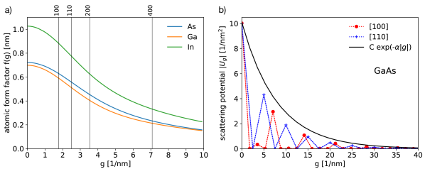
Figure 5: Atomic form factors and scattering potential:  a) atomic form factors in dependence on the wave vector $g$ for Ga, As, and In following [24]. The vertical lines indicate positions of the lattice planes (100), (110), (200) and (400) in GaAs.
b) Fourier coefficients of the scattering potential for GaAs along the [100]- (red) and [110]-crystallographic directions (blue) as computed by pyTEM [15] using (22). The blue and red lines are only for guiding of the eye. An exponential decay (solid black) as assumed in (21) can be observed with $C=10.1\,\mathrm{1/nm^{2}}$ and $\alpha=0.125\ \mathrm{nm}$.

With this assumption we are now able to control the size of the solutions of (16) in the weighted norm if $|\alpha|<\alpha_{\mathbb{U}}$. In the following result $\alpha$ may be positive or negative, but later on we are interested in $\alpha>0$.

Theorem 3.5 (Weighted norms).

Consider the DHW_G as in (19) with ${\mathbf{G}}\subset{\mathbf{G}}_{\gamma}\subset\Lambda^{*}$ with $\gamma\in{]0,1[}$. Moreover, assume that ${\mathcal{U}}$ satisfies (21). Then, for all $\alpha\in{]{-}\alpha_{\mathbb{U}},\alpha_{\mathbb{U}}[}$ and all initial conditions ${\bm{\psi}}^{0}\in\mathfrak{H}({\mathbf{G}})$ with $\|{\bm{\psi}}^{0}\|_{\alpha}<\infty$ the unique solution ${\bm{\psi}}$ of (19) with ${\bm{\psi}}(0)={\bm{\psi}}^{0}$ satisfies the estimate

(23) $$\|{\bm{\psi}}(z)\|_{\alpha}\leq\mathrm{e}^{\kappa(\alpha)|z|}\|{\bm{\psi}}^{0}\|_{\alpha}\quad\text{for }z\in{\mathbb{R}},$$

where the exponential growth rate $\kappa(\alpha)$ is explicitly given by

$$\kappa(\alpha)=\frac{\pi C_{\mathbb{U}}}{\gamma\rho_{0}}\>|\alpha|\;\!\mathfrak{S}_{1}(\alpha_{\mathbb{U}}{-}|\alpha|),\quad\text{where }\mathfrak{S}_{m}(\beta):=\sum_{\varkappa\in\Lambda^{*}}|\varkappa|^{m}\mathrm{e}^{-\beta|\varkappa|}\,.$$

Proof 3.6.

Step 1. Transformation of the equation: We introduce the new variables $B_{g}=\mathrm{e}^{\alpha|g|}\psi_{g}$ such that $\|{\bm{\psi}}\|_{\alpha}=\|B\|_{\mathbf{G}}$. In terms of $B$ we can rewrite DHW_G as

(24) $$\mathrm{i}R\overset{\text{\LARGE.}}{B}+\Sigma B=-{\mathbb{U}}^{(\alpha)}B=-{\mathbb{U}}B+{\mathbb{P}}^{(\alpha)}B\ \text{ with }{\mathbb{P}}^{(\alpha)}_{g,h}=\big{(}1-\mathrm{e}^{\alpha(|g|-|h|)}\big{)}U_{g-h}.$$

Here we used that $R$ and $\Sigma$ are diagonal operators, and hence commute with the multiplication of the exponential factor. Using the bound (21) for $U_{g}$, the coefficients of the perturbation operator ${\mathbb{P}}^{(\alpha)}$ can be bounded by

(25) $$|{\mathbb{P}}^{(\alpha)}_{g,h}|\leq C_{\mathbb{U}}\big{(}1-\mathrm{e}^{|\alpha|\,|g-h|}\big{)}\mathrm{e}^{-\alpha_{\mathbb{U}}|g-h|}\leq C_{\mathbb{U}}\,\min\{1,|\alpha|\,|g{-}h|\}\,\mathrm{e}^{-(\alpha_{\mathbb{U}}{-}|\alpha|)|g-h|}.$$

Step 2. Operator norm of $R^{-1}{\mathbb{P}}^{(\alpha)}$ in $\mathfrak{H}({\mathbf{G}})$. To control the perturbation $R^{-1}{\mathbb{P}}^{(\alpha)}B$ in terms of $\|B\|_{\mathbf{G}}$ we employ Lemma 3.7 to obtain $\|R^{-1}{\mathbb{P}}^{(\alpha)}B\|_{\mathbf{G}}\leq C^{(\alpha)}_{\mathbb{P}}\|B\|_{\mathbf{G}}$ with

$$C^{(\alpha)}_{\mathbb{P}}:=\Big{(}\sup_{g\in{\mathbf{G}}}\sum_{h\in{\mathbf{G}}}\frac{\pi|{\mathbb{P}}_{g,h}^{(\alpha)}|}{|\rho_{g}\rho_{h}|^{1/2}}\Big{)}^{1/2}\Big{(}\sup_{h\in{\mathbf{G}}}\sum_{g\in{\mathbf{G}}}\frac{\pi|{\mathbb{P}}_{g,h}^{(\alpha)}|}{|\rho_{g}\rho_{h}|^{1/2}}\Big{)}^{1/2}.$$

Because of $\rho_{g},\rho_{h}\in{\mathbf{G}}\subset{\mathbf{G}}_{\gamma}$, and (25) this yields

$$C^{(\alpha)}_{\mathbb{P}} \leq\pi C_{\mathbb{U}}\>\sup_{g\in{\mathbf{G}}}\sum_{h\in{\mathbf{G}}}\frac{|\alpha|\,|g{-}h|}{\gamma\rho_{0}}\>\mathrm{e}^{-(\alpha_{\mathbb{U}}{-}|\alpha|)|g-h|}\ \leq\ \frac{\pi C_{\mathbb{U}}}{\gamma\rho_{0}}\>|\alpha|\!\;\mathfrak{S}_{1}(\alpha_{\mathbb{U}}{-}\alpha)\ =\ \kappa(\alpha).$$

Step 3. Gronwall estimate. We now apply the variation-of-constants formula (Duhamel’s principle) to the solution $B$ for (24) in the $\mathfrak{H}({\mathbf{G}})$, where $H=R^{-1}(\Sigma{-}{\mathbb{U}})$ is the generator of the norm-preserving $C_{0}$ group $\mathrm{e}^{\mathrm{i}zH}$:

$$\|B(z)\|_{\mathbf{G}} \leq\|\mathrm{e}^{iHz}B(0)\|_{\mathbf{G}}+\int_{0}^{z}\|\mathrm{e}^{i(z-\zeta)H}\|_{\mathbf{G}}\|R^{-1}{\mathbb{P}}^{(\alpha)}B(\zeta)\|_{\mathbf{G}}\;\!\mathrm{d}\zeta$$

$$\leq\|{\bm{\psi}}(0)\|_{\alpha}+\int_{0}^{z}\kappa(\alpha)\,\|B(\zeta)\|_{\mathbf{G}}\;\!\mathrm{d}\zeta.$$

Now, Gronwall’s estimate gives $\|{\bm{\psi}}(z)\|_{\alpha}=\|B(z)\|_{\mathbf{G}}\leq\mathrm{e}^{\kappa(\alpha)z}\|{\bm{\psi}}(0)\|_{\alpha}$, and the proof is completed.

Step 2 of the above proof relies on the following elementary lemma, which will be used again to calculate the norm of convolution-type operators involving ${\mathbb{U}}$.

Lemma 3.7 (Operator norm).

Consider ${\mathbf{G}}^{(1)},{\mathbf{G}}^{(2)}\subset{\mathbf{G}}_{\gamma}$ with $\gamma>0$ and ${\mathbb{B}}:\mathfrak{H}({\mathbf{G}}^{(1)})\to\mathfrak{H}({\mathbf{G}}^{(2)})$ with $({\mathbb{B}}A)_{g}=\sum_{h\in{\mathbf{G}}^{(1)}}B_{gh}A_{h}$. Setting $\widetilde{B}_{gh}=\sqrt{\rho_{g}/\rho_{h}}\,B_{gh}$ gives

(26) $$\|{\mathbb{B}}A\|_{{\mathbf{G}}^{(2)}}\leq C_{\mathbb{B}}\|A\|_{{\mathbf{G}}^{(1)}},\ \ C_{\mathbb{B}}=\Big{(}\!\sup_{h\in{\mathbf{G}}^{(1)}}\!\sum_{g\in{\mathbf{G}}^{(2)}}\!\!|\widetilde{B}_{gh}|\Big{)}^{1/2}\Big{(}\!\sup_{g\in{\mathbf{G}}^{(2)}}\!\sum_{h\in{\mathbf{G}}^{(1)}}\!\!|\widetilde{B}_{gh}|\Big{)}^{1/2}\!,$$

which is the square root of the product of the row-sum and column-sum norm.

Proof 3.8.

With $r_{g}=\rho_{g}^{1/2}$ the desired result is obtained as follows:

$$\|{\mathbb{B}}A\|_{{\mathbf{G}}^{(2)}}^{2} =\!\!\sum_{g\in{\mathbf{G}}^{(2)}}\!\!r_{g}^{2}\Big{(}\!\sum_{h\in{\mathbf{G}}^{(1)}}\!\!\!B_{gh}A_{h}\Big{)}\overline{({\mathbb{B}}A)}_{g}\leq\!\!\sum_{g\in{\mathbf{G}}^{(2)}}\sum_{h\in{\mathbf{G}}^{(1)}}\!\!\!r_{h}|\widetilde{B}_{gh}|^{1/2}|A_{h}|r_{g}|\widetilde{B}_{gh}|^{1/2}|({\mathbb{B}}A)_{g}|$$

$$\leq_{\mathrm{CaSch}}\Big{(}\sum_{g\in{\mathbf{G}}^{(2)}}\sum_{h\in{\mathbf{G}}^{(1)}}\!\!|\widetilde{B}_{gh}|\,r_{h}^{2}|A_{h}|^{2}\Big{)}^{1/2}\Big{(}\sum_{g\in{\mathbf{G}}^{(2)}}\sum_{h\in{\mathbf{G}}^{(1)}}\!\!|\widetilde{B}_{gh}|\,r_{g}^{2}|({\mathbb{B}}A)_{g}|^{2}\Big{)}^{1/2}$$

$$\leq\ \Big{(}\sup_{h\in{\mathbf{G}}^{(1)}}\big{(}\sum_{g\in{\mathbf{G}}^{(2)}}\!\!|\widetilde{B}_{gh}|\big{)}\Big{)}^{1/2}\|A\|_{{\mathbf{G}}^{(1)}}\ \Big{(}\sup_{g\in{\mathbf{G}}^{(2)}}\big{(}\sum_{h\in{\mathbf{G}}^{(1)}}\!\!|\widetilde{B}_{gh}|\big{)}\Big{)}^{1/2}\,\|{\mathbb{B}}A\|_{{\mathbf{G}}^{(2)}}$$

$$\ =\ C_{\mathbb{B}}\|A\|_{{\mathbf{G}}^{(1)}}\|{\mathbb{B}}A\|_{{\mathbf{G}}^{(2)}}.$$

Thus, Lemma 3.7 is established.

The importance of Theorem 3.5 is that the growth rate $\kappa(\alpha)$ is completely independent of the domain ${\mathbf{G}}$ as long as ${\mathbf{G}}$ is contained in ${\mathbf{G}}_{\gamma}$. Thus, we will have the option to compare solutions obtained for different wave-vector sets ${\mathbf{G}}$.

As a first consequence we obtain that for all $z\in[0,z_{*}]$ the solutions ${\bm{\psi}}(z)=(\psi_{g}(z))_{g\in{\mathbf{G}}}$ decay with $|g|\to\infty$. Indeed, recalling that the initial condition is given by the incoming wave encoded in the ${\bm{\delta}}=(\delta_{0,g})_{g\in{\mathbf{G}}}$ (Kronecker symbol) we have

(27) $$\|{\bm{\psi}}(0)\|_{\alpha}=\|{\bm{\psi}}(0)\|_{\mathbf{G}}=\|{\bm{\delta}}\|_{\mathbf{G}}=\sqrt{\rho_{0}}=\sqrt{k_{0}\cdot{\bm{\nu}}}\approx\sqrt{|k_{0}|},$$

which is independent of the exponential weighting by $\alpha$. With this and $\alpha\in{]0,\alpha_{\mathbb{U}}[}$ we obtain

$$|\psi_{g}(z)|\ \leq\ \frac{\mathrm{e}^{-\alpha|g|}}{\sqrt{\rho_{g}}}\|{\bm{\psi}}(z)\|_{\alpha}\ \leq\ \mathrm{e}^{\kappa(\alpha)|z|-\alpha|g|}\sqrt{\frac{\rho_{0}}{\rho_{g}}}.$$

Thus, the exponential factor $\mathrm{e}^{\kappa(\alpha)|z|-\alpha|g|}$ shows that the solution ${\bm{\psi}}(z)$ can only have a nontrivial effect at $g\neq 0$ if $|z|>\alpha/\kappa(\alpha)\>|g|$. We may consider the quotient $\alpha/\kappa(\alpha)$ as a collective scattering length that describes how fast a beam has to travel through the specimen to generate nontrivial amplitudes at neighboring wave vectors $g$. In contrast, the extinction length $\xi_{g}$ is defined for each individual $g\in\Lambda^{*}$ (see [3, p.309]):

$$\frac{\alpha}{\kappa(\alpha)}=\frac{\gamma\,k_{0}\cdot{\bm{\nu}}}{\pi C_{\mathbb{U}}\mathfrak{S}_{1}(\alpha_{\mathbb{U}}{-}\alpha)}\quad\text{versus the extinction length }\xi_{g}:=\frac{|\rho_{g}|}{|U_{g}|}.$$

Hence, for doing a reasonable TEM experiment, one wants $\kappa(\alpha)z_{*}$ to be big enough to see some effect of scattering. However, it should not be too big such that the radius of possibly activated wave vectors with $|\psi_{g}|\geq\varepsilon$ is not too small, namely those with $|g|\leq\frac{1}{\alpha}\big{(}\kappa(\alpha)z_{*}+\log(1/\varepsilon)\big{)}$. In addition we define the excitation length to be $\ell_{\mathrm{excit}}(s_{g})=1/|s_{g}|$, which describes the period of the phase oscillation of $\psi_{g}(t)$.

3.3 Error estimates for finite-dimensional approximations

We now compare the DHW equations on different sets ${\mathbf{G}}^{(1)}$ and ${\mathbf{G}}^{(2)}$, both contained in ${\mathbf{G}}_{\gamma}\subset\Lambda^{*}$. We denote by ${\bm{\psi}}^{(j)}$ the solution of DHW${}_{{\mathbf{G}}^{(j)}}$ with the initial condition ${\bm{\psi}}^{(j)}(0)={\bm{\delta}}$.

Assuming ${\mathbf{G}}^{(1)}\subset{\mathbf{G}}^{(2)}$ we can decompose ${\bm{\psi}}^{(2)}$ into two pieces, namely

$${\bm{\psi}}^{(2)}=(B,C)\quad\text{with }B={\bm{\psi}}^{(2)}|_{{\mathbf{G}}^{(1)}}:=(\psi_{g})_{g\in{\mathbf{G}}^{(1)}}\text{ and }C={\bm{\psi}}^{(2)}|_{{\mathbf{G}}^{(2)}\setminus{\mathbf{G}}^{(1)}}.$$

We may rewrite the DHW${}_{{\mathbf{G}}^{(2)}}$ in block structure via

(28a) $$R_{(1)}\overset{\text{\LARGE.}}{B}\ \ =\mathrm{i}\big{(}\ \ \Sigma_{(1)}B\ \ +{\mathbb{U}}_{BB}B+{\mathbb{U}}_{BC}C\big{)}, B(0)=(\delta_{0,g})_{g\in{\mathbf{G}}^{(1)}}$$

(28b) $$R_{(2)\setminus(1)}\overset{\text{\LARGE.}}{C} =\mathrm{i}\big{(}\Sigma_{(2)\setminus(1)}B+{\mathbb{U}}_{CB}B+{\mathbb{U}}_{CC}C\big{)}, C(0)=0.$$

Here we used that the initial conditions ${\bm{\psi}}(0)$ is localized in the incoming beam such that $\psi_{g}(0)=0$ for $g\in{\mathbf{G}}^{(2)}\setminus{\mathbf{G}}^{(1)}$. Moreover, the DHW${}_{{\mathbf{G}}^{(1)}}$ is given by (28a) if we omit the coupling term “ $+{\mathbb{U}}_{BC}C$ ”:

(29) $$R_{(1)}M\overset{\text{\LARGE.}}{{\bm{\psi}}}^{(1)}=\mathrm{i}\,\big{(}\Sigma_{(1)}+{\mathbb{U}}_{BB}\big{)}{\bm{\psi}}^{(1)},\quad{\bm{\psi}}^{(1)}(0)=(\delta_{0,g})_{g\in{\mathbf{G}}^{M}}.$$

The following result provides a first estimate between the solution ${\bm{\psi}}^{(2)}=(B,C)$ on the larger wave-vector set ${\mathbf{G}}^{(2)}$ and ${\bm{\psi}}^{(1)}$ on the smaller set ${\mathbf{G}}^{(1)}$ by exploiting the exponential decay estimates established in Theorem 3.5. In this first case, we consider only the model sets ${\mathbf{G}}^{(1)}={\mathbf{G}}^{M}$ and ${\mathbf{G}}^{(2)}={\mathbf{G}}_{\gamma}$ with ${\mathbf{G}}^{M}\subset{\mathbf{G}}_{\gamma}$, see (18).

Theorem 3.9 (Control of approximation errors).

Assume that the assumptions (15) and (21) hold and that $k_{0}$, $M$ and $\gamma\in{]0,1[}$ are such that ${\mathbf{G}}^{M}\subset{\mathbf{G}}_{\gamma}$. Then, for $\alpha\in{]0,\alpha_{\mathbb{U}}[}$ the solutions ${\bm{\psi}}^{\gamma}$ and ${\bm{\psi}}^{M}$ of DHW${}_{{\mathbf{G}}_{\gamma}}$ and DHW${}_{{\mathbf{G}}^{M}}$ with initial condition ${\bm{\delta}}$ satisfy the estimates

(30a) $$\big{\|}{\bm{\psi}}^{M}(z)-{\bm{\psi}}^{\gamma}(z)|_{{\mathbf{G}}^{M}}\big{\|}_{{\mathbf{G}}^{M}} \leq\frac{\mathfrak{S}_{0}(\alpha_{\mathbb{U}})-1}{\alpha\,\mathfrak{S}_{1}(\alpha_{\mathbb{U}}{-}\alpha)}\>\mathrm{e}^{\kappa(\alpha)|z|-\alpha M}\>\|{\bm{\delta}}\|_{0}\ \ \text{ and }$$

(30b) $$\big{\|}{\bm{\psi}}^{\gamma}(z)|_{{\mathbf{G}}_{\gamma}\setminus{\mathbf{G}}^{M}}\big{\|}_{{\mathbf{G}}_{\gamma}\setminus{\mathbf{G}}^{M}}\ \ \leq\mathrm{e}^{\kappa(\alpha)|z|-\alpha M}\|{\bm{\delta}}\|_{0}\quad\text{for all }z\in{\mathbb{R}}.$$

where as before $\mathfrak{S}_{m}(\beta):=\sum_{\varkappa\in\Lambda^{*}}|\varkappa|^{m}\,\mathrm{e}^{-\beta|\varkappa|}$.

Proof 3.10.

We denote by ${\mathbf{G}}_{\mathrm{O}}:={\mathbf{G}}_{\gamma}\setminus{\mathbf{G}}^{M}$ the set of outer wave vectors.

Step 1: Estimate of $C$. The solution ${\bm{\psi}}^{\gamma}=(B,C)$ satisfies all assumptions of Theorem 3.5. Hence, we can rely on the exponential estimate and obtain

$$\|C(z)\|_{{\mathbf{G}}_{\mathrm{O}}}^{2}\ =\ \sum_{h\in{\mathbf{G}}_{\mathrm{O}}}\rho_{h}\,|\psi_{h}(z)|^{2}\ \leq\ \mathrm{e}^{-2\alpha M}\sum_{g\in{\mathbf{G}}_{\gamma}}\rho_{g}\,\mathrm{e}^{2\alpha|g|}\,|\psi_{g}(z)|^{2}$$

$$=\ \mathrm{e}^{-2\alpha M}\|{\bm{\psi}}^{M}(z)\|_{\alpha}^{2}\ \leq\ \mathrm{e}^{2\kappa(\alpha)|z|-2\alpha M}\|{\bm{\psi}}^{M}(0)\|_{\alpha}^{2}\ =\ \mathrm{e}^{2\kappa(\alpha)|z|-2\alpha M}\|{\bm{\delta}}\|_{0}^{2},$$

which is the desired result (30b).

Step 2. Estimate between $B$ and ${\bm{\psi}}^{M}$. For comparing $B$ and ${\bm{\psi}}^{M}$ we define $A=B-{\bm{\psi}}^{M}$ and see that $A$ satisfies

(31) $$R_{M}\overset{\text{\LARGE.}}{A}(z)=\mathrm{i}\big{(}\Sigma_{M}A(z)+{\mathbb{U}}_{BB}A(z)+{\mathbb{U}}_{BC}C(z)\big{)},\qquad A(0)=0,$$

where now the initial condition is $0$. Using the unitary group $\mathrm{e}^{\mathrm{i}zH_{M}}$ on $\mathfrak{H}({\mathbf{G}}^{M})$ defined via $H_{M}=R_{M}^{-1}(\Sigma_{M}{+}{\mathbb{U}}_{BB})$, the solution is given in terms of Duhamel’s principle via $A(z)=\int_{0}^{z}\mathrm{e}^{\mathrm{i}(z{-}\zeta)H_{M}}R_{M}^{-1}{\mathbb{U}}_{BC}C(\zeta)\;\!\mathrm{d}\zeta$. Taking the norm in $\mathfrak{H}({\mathbf{G}}^{M})$ we arrive at

$$\|A(z)\|_{{\mathbf{G}}^{M}}\leq\!\int_{0}^{z}\!\!\|R_{M}^{-1}{\mathbb{U}}_{BC}C(\zeta)\|_{{\mathbf{G}}^{M}}\;\!\mathrm{d}\zeta\leq\|R_{M}^{-1}{\mathbb{U}}_{BC}\|_{\mathfrak{H}({\mathbf{G}}_{\mathrm{O}}){\to}\mathfrak{H}({\mathbf{G}}^{M})}\!\int_{0}^{z}\!\|C(\zeta)\|_{{\mathbf{G}}_{\mathrm{O}}}\;\!\mathrm{d}\zeta.$$

Using Lemma 3.7, the operator norm $N_{\mathrm{cpl}}=\|R_{M}^{-1}{\mathbb{U}}_{BC}\|$ can be estimated by

$$N_{\mathrm{cpl}}\leq\Big{(}\sup_{h\in{\mathbf{G}}^{M}}\!\sum_{g\in{\mathbf{G}}_{\mathrm{O}}}\!\!\!\tfrac{\pi|U_{g-h}|}{\sqrt{\rho_{g}\rho_{h}}}\Big{)}^{1/2}\Big{(}\sup_{g\in{\mathbf{G}}_{\mathrm{O}}}\!\sum_{h\in{\mathbf{G}}^{M}}\!\!\!\tfrac{\pi|U_{g-h}|}{\sqrt{\rho_{g}\rho_{h}}}\Big{)}^{1/2}\!\leq\tfrac{\pi}{\gamma\rho_{0}}\sup_{g\in\Lambda^{*}}\!\sum_{h\in\Lambda^{*}\setminus\{g\}}\!\!\!\!C_{\mathbb{U}}\mathrm{e}^{-\alpha_{\mathbb{U}}|g{-}h|},$$

where we used $g\in{\mathbf{G}}_{\gamma}$ and (21). We also increased the sets ${\mathbf{G}}^{M}$ and ${\mathbf{G}}_{\mathrm{O}}$ but kept the information that they are disjoint by summing only over $h$ different from $g$. Thus, we find $N_{\mathrm{cpl}}\leq\pi C_{\mathbb{U}}\big{(}\mathfrak{S}_{0}(\alpha_{\mathbb{U}})-1\big{)}/(\gamma\rho_{0})$.

Inserting this into the bound for $\|A(z)\|_{{\mathbf{G}}^{M}}$ and integrating the bound (30b) for $C(\zeta)$ we see cancellations in the factor $N_{\mathrm{cpl}}/\kappa(\alpha)$, and the result (30a) follows.

The next result is dedicated to the case of two general sets ${\mathbf{G}}^{(1)}$ and ${\mathbf{G}}^{(2)}$ both of which satisfy ${\mathbf{G}}^{M}\subset{\mathbf{G}}^{(j)}\subset{\mathbf{G}}_{\gamma}$ for $j=1,2$. Denoting by ${\bm{\psi}}^{(j)}:[0,z_{*}]\to\mathfrak{H}({\mathbf{G}}^{(j)})$ the solutions of DHW${}_{{\mathbf{G}}^{(j)}}$, we will see that their restrictions to ${\mathbf{G}}^{M}$ will be exponentially close with a factor $\mathrm{e}^{-\alpha M}$. This explains why the exact choice of the subset ${\mathbf{G}}$ of the wave vectors is not relevant for $z\in[0,z_{*}]$ as long as it contains a sufficiently large subset ${\mathbf{G}}^{M}$, i.e. $M$ is much larger than $\kappa(\alpha)z_{*}/\alpha$.

Corollary 3.11 (Arbitrary sets ${\mathbf{G}}^{(j)}$ of wave vectors).

Consider $k_{0}$, $\gamma$, and $M$ as in Theorem 3.9 and consider two subsets ${\mathbf{G}}^{(j)}\subset\Lambda^{*}$ satisfying ${\mathbf{G}}^{M}\subset{\mathbf{G}}^{(j)}\subset{\mathbf{G}}_{\gamma}$ for $j=1,2$. Then, the solutions ${\bm{\psi}}^{(j)}$ of DHW${}_{{\mathbf{G}}^{(j)}}$ with initial condition ${\bm{\psi}}^{(j)}(0)={\bm{\delta}}$ satisfy the estimate

$$\big{\|}{\bm{\psi}}^{(1)}(z)|_{{\mathbf{G}}^{M}}-{\bm{\psi}}^{(2)}(z)|_{{\mathbf{G}}^{M}}\big{\|}_{{\mathbf{G}}^{M}}\leq\frac{2\>\big{(}\mathfrak{S}_{0}(\alpha_{\mathbb{U}})-1\big{)}}{\alpha\,\mathfrak{S}_{1}(\alpha_{\mathbb{U}}{-}\alpha)}\>\mathrm{e}^{\kappa(\alpha)|z|-\alpha M}\,\|{\bm{\delta}}\|_{0}\quad\text{for all }z\in{\mathbb{R}}\,.$$

Proof 3.12.

The proof follows simply by observing that Theorem 3.9 can easily be generalized by replacing the bigger set ${\mathbf{G}}_{\gamma}$ by any set ${\mathbf{G}}$ between ${\mathbf{G}}^{M}$ and ${\mathbf{G}}_{\gamma}$. Hence, we can compare the two solutions ${\bm{\psi}}^{(j)}$ on ${\mathbf{G}}^{M}$ with the solution ${\bm{\psi}}^{M}$ of DHW${}_{{\mathbf{G}}^{M}}$. Now the result follows by

$$\|{\bm{\psi}}^{(1)}|_{{\mathbf{G}}^{M}}-{\bm{\psi}}^{(2)}|_{{\mathbf{G}}^{M}}\|_{{\mathbf{G}}^{M}}\leq\|{\bm{\psi}}^{(1)}|_{{\mathbf{G}}^{M}}-{\bm{\psi}}^{M}\|_{{\mathbf{G}}^{M}}+\|{\bm{\psi}}^{M}-{\bm{\psi}}^{(2)}|_{{\mathbf{G}}^{M}}\|_{{\mathbf{G}}^{M}}$$

and applying (30a) with $\|{\bm{\psi}}(0)\|_{\alpha}=\|{\bm{\delta}}\|_{0}=\rho_{0}^{1/2}$.

From now on we will always choose $\alpha=\alpha_{\mathbb{U}}/2$, which is the intermediate value that makes all sums $\mathfrak{S}_{m}\big{(}\alpha_{\mathbb{U}}/2\big{)}$ finite. Thus, the critical exponential error term takes the form

$$\mathrm{e}^{\kappa(\alpha_{\mathbb{U}}/2)z-M\alpha_{\mathbb{U}}/2}\quad\text{for }z\in[0,z_{*}].$$

From practical purposes there is no reason of doing a calculation in a set ${\mathbf{G}}$ bigger than ${\mathbf{G}}^{M}$, since increasing the number of ODEs without a gain in accuracy is useless. Moreover, it is desirable to reduce $M$ as much as possible as the number of ODEs in DHW${}_{{\mathbf{G}}^{M}}$ with $M=\mu|k_{0}|$ is proportional to $M^{d}$. However, in a true experiment we want to see the effect of scattering such that $\kappa(\alpha)z_{*}$ needs to be big enough. The way to make this work is to choose $M$ proportional to a small power of $|k_{0}|$:

$$M\sim|k_{0}|^{\eta}\quad\text{with }\eta\in{]0,1[}.$$

For instance the first few Laue zones (see below) can be obtained by $\eta=1/2$.

While in a ball ${\mathbf{G}}^{M}$ of radius $M$ the number of wave vectors scales with $M^{d}$, there are further physical reasons that many of these wave vectors are not relevant, as they cannot be activated because of energetic criteria as discussed now.

3.4 Averaging via conservation of the energy norm

The relevance of the Ewald sphere lies in the fact that on ${\mathbb{S}}_{\mathrm{Ew}}$ the excitation error $s_{g}=\sigma_{g}/(2\rho_{g})$ equals $0$. This means that beams propagating with wave vectors $g\in{\mathbb{S}}_{\mathrm{Ew}}$ have much lower energy, because they have only little phase oscillations. Beams with wave vectors that are not close to the Ewald sphere will necessarily have much smaller amplitudes, because they have much larger phase oscillations than beams with wave vectors near the Ewald sphere. Mathematically this can be manifested by conservation of suitable energies. Another way of obtaining this result would be by performing a temporal averaging for the functions $\psi_{g}$ with large $|s_{g}|$.

We return to the DHW equations on ${\mathbf{G}}={\mathbf{G}}^{M}\subset{\mathbf{G}}_{\gamma}$. The linear finite-dimensional Hamiltonian system

(32) $$R\overset{\text{\LARGE.}}{{\bm{\psi}}}=\mathrm{i}\big{(}\Sigma{+}{\mathbb{U}}\big{)}{\bm{\psi}},\quad{\bm{\psi}}(0)={\bm{\delta}}\in\mathfrak{H}({\mathbf{G}}^{M}),$$

can be rewritten via the transformation $\widetilde{R}=R^{1/2}=\mathop{\mathrm{diag}}\big{(}(\rho_{g}/\pi)^{1/2}\big{)}_{g\in{\mathbf{G}}}$. Setting $A=\widetilde{R}{\bm{\psi}}$, system (32) takes the standard Hamiltonian form

(33) $$\overset{\text{\LARGE.}}{A}=\mathrm{i}\,{\mathbb{H}}A\quad\text{with }{\mathbb{H}}=\widetilde{R}^{-1}\,\big{(}\Sigma{+}{\mathbb{U}}\big{)}\,\widetilde{R}^{-1},$$

where ${\mathbb{H}}$ is now a Hermitian operator on $\ell^{2}({\mathbf{G}}^{M})$, now using the standard scalar product. This provides the explicit solution $A(z)=\mathrm{e}^{\mathrm{i}z{\mathbb{H}}}A(0)$ via the unitary group $z\mapsto\mathrm{e}^{\mathrm{i}z{\mathbb{H}}}$. An easy consequence is the invariance of the hierarchy of norms:

$$\forall\,k\in{\mathbb{N}}_{0}\ \forall\,z\in{\mathbb{R}}:\quad\big{\langle}{\mathbb{H}}^{k}A(z),A(z)\big{\rangle}=\big{\langle}{\mathbb{H}}^{k}A(0),A(0)\big{\rangle}\,.$$

For $k=0$ this is the simple wave-flux conservation established in Proposition 3.1. The result for $k=1$ is not useful, because the operator ${\mathbb{H}}$ is indefinite, since ${\mathbb{U}}$ is bounded and $\Sigma$ has many positive (associated with $g$ inside the Ewald sphere) and many negative eigenvalues (associated with $g$ outside the Ewald sphere).

Hence, we concentrate on the case $k=2$, where

$$0\leq{\mathbb{H}}^{2}=\widetilde{\Sigma}^{2}+\widetilde{\mathbb{U}}\widetilde{\Sigma}+\widetilde{\Sigma}\widetilde{\mathbb{U}}+\widetilde{\mathbb{U}}^{2},\quad\text{with }\widetilde{\Sigma}:=\widetilde{R}^{-1}\Sigma\widetilde{R}^{-1}=R^{-1}\Sigma\text{ and }\widetilde{\mathbb{U}}:=\widetilde{R}^{-1}{\mathbb{U}}\widetilde{R}^{-1}.$$

The following, rather trivial result highlights that ${\mathbb{H}}^{2}$ has suitable definiteness properties that will then be useful for estimating the solutions of the DHW equations.

Lemma 3.13 (Energy estimate).

Let ${\mathbb{H}}=\widetilde{\Sigma}+\widetilde{\mathbb{U}}$ where $\widetilde{\Sigma}$ and ${\mathbb{H}}$ are Hermitian, then we have the estimate

(34) $$\|{\mathbb{H}}A\|^{2} =\big{\langle}{\mathbb{H}}^{2}A,A\big{\rangle}\geq\frac{1}{2}\|\widetilde{\Sigma}A\|^{2}-\|\widetilde{\mathbb{U}}A\|^{2}\quad\text{for all }A\in\ell^{2}({\mathbf{G}}^{M}).$$

Proof 3.14.

We expand ${\mathbb{H}}^{2}$ in a suitable way:

$${\mathbb{H}}^{2} =(\widetilde{\Sigma}+\widetilde{\mathbb{U}})^{2}=\frac{1}{2}\widetilde{\Sigma}{}^{2}+\big{(}\frac{1}{2}\widetilde{\Sigma}{}^{2}+\widetilde{\Sigma}\widetilde{\mathbb{U}}+\widetilde{\mathbb{U}}\widetilde{\Sigma}+2\widetilde{\mathbb{U}}{}^{2}\big{)}-\widetilde{\mathbb{U}}{}^{2}$$

$$=\frac{1}{2}\widetilde{\Sigma}{}^{2}+\Big{(}\frac{1}{\sqrt{2}}\widetilde{\Sigma}+\sqrt{2}\widetilde{\mathbb{U}}\Big{)}^{2}-\widetilde{\mathbb{U}}{}^{2}\ \geq\ \frac{1}{2}\widetilde{\Sigma}{}^{2}-\widetilde{\mathbb{U}}{}^{2}.$$

This is the desired result.

It is instructive to transform estimate (34) back to the original variable ${\bm{\psi}}$ and the operator $H=R^{-1}(\Sigma{+}{\mathbb{U}})$, which yields

(35) $$\|R^{-1}\Sigma{\bm{\psi}}\|_{{\mathbf{G}}^{M}}^{2}\ \leq\ 2\,\|H{\bm{\psi}}\|^{2}_{{\mathbf{G}}^{M}}+2\,\|R^{-1}{\mathbb{U}}{\bm{\psi}}\|_{{\mathbf{G}}^{M}}^{2}.$$

Since along solutions $z\mapsto{\bm{\psi}}(z)\in\mathfrak{H}({\mathbf{G}}^{M})$ of DHW${}_{{\mathbf{G}}^{M}}$ the energy $\|H{\bm{\psi}}(z)\|^{2}_{{\mathbf{G}}^{M}}$ is constant, see (20), we can use this for bounding $\|R^{-1}\Sigma{\bm{\psi}}(z)\|_{{\mathbf{G}}^{M}}^{2}$.

Proposition 3.15 (Energy bound for solutions).

Consider $k_{0}$, $\gamma$, and $M$ such that ${\mathbf{G}}^{M}\subset{\mathbf{G}}_{\gamma}$. Let ${\bm{\psi}}$ be the solution of DHW${}_{{\mathbf{G}}^{M}}$ with initial condition ${\bm{\psi}}(0)={\bm{\delta}}$. Then, ${\bm{\psi}}$ satisfies the estimate

$$\|R^{-1}\Sigma{\bm{\psi}}(z)\|_{{\mathbf{G}}^{M}}\leq\frac{2\pi\;\!C_{\mathbb{U}}\mathfrak{S}_{0}(\alpha_{\mathbb{U}})}{\gamma\rho_{0}}\|{\bm{\delta}}\|_{{\mathbf{G}}^{M}}\quad\text{for all }z\in{\mathbb{R}}.$$

Proof 3.16.

Lemma 3.7 yields $\|R^{-1}{\mathbb{U}}{\bm{\psi}}\|_{{\mathbf{G}}^{M}}\leq{\widehat{c}_{\mathbb{U}}}\|{\bm{\psi}}\|_{{\mathbf{G}}^{M}}$ with ${\widehat{c}_{\mathbb{U}}}=\pi\;\!C_{\mathbb{U}}\mathfrak{S}_{0}(\alpha_{\mathbb{U}})/(\gamma\rho_{0})$. Exploiting (35) and the conservation of $\|H{\bm{\psi}}(z)\|^{2}_{{\mathbf{G}}^{M}}$ and $\|{\bm{\psi}}(z)\|_{{\mathbf{G}}^{M}}^{2}$ we find

$$\|R^{-1}\Sigma{\bm{\psi}}(z)\|_{{\mathbf{G}}^{M}}^{2} \leq 2\|H{\bm{\psi}}(z)\|^{2}_{{\mathbf{G}}^{M}}{+}2{\widehat{c}_{\mathbb{U}}^{2}}\|{\bm{\psi}}(z)\|_{{\mathbf{G}}^{M}}^{2}$$

$$=2\|H{\bm{\psi}}(0)\|^{2}_{{\mathbf{G}}^{M}}{+}2{\widehat{c}_{\mathbb{U}}^{2}}\|{\bm{\psi}}(0)\|_{{\mathbf{G}}^{M}}^{2}=2\|R^{-1}{\mathbb{U}}{\bm{\delta}}\|^{2}_{{\mathbf{G}}^{M}}{+}2{\widehat{c}_{\mathbb{U}}^{2}}\rho_{0}\leq 4{\widehat{c}_{\mathbb{U}}^{2}}\rho_{0},$$

where we used ${\bm{\psi}}(0)={\bm{\delta}}$ and $\sigma_{0}=0$. This shows the desired assertion.

Figure 6: Ewald sphere ${\mathbb{S}}_{\mathrm{Ew}}$ (blue), dual lattice $\Lambda^{*}$ (black dots), and the decomposition of ${\mathbf{G}}^{M}$ (light red ball) into ${\mathbf{G}}^{M}_{\mathrm{Ew}}$ (red annular arc, for $\widetilde{s}_{*}=3\pi$) and ${\mathbf{G}}^{M}_{\mathrm{far}}$. The boxes indicate the Laue zones: lowest order (yellow) to third order (green).

Using the energy bound, we can split the set ${\mathbf{G}}^{M}$ according to the size of the excitation errors $s_{g}=\sigma_{g}/(2\rho_{g})$ using a cut-off value $\widetilde{s}_{*}$ to be chosen later:

$${\mathbf{G}}^{M}={\mathbf{G}}^{M}_{\mathrm{Ew}}\,\overset{\text{\LARGE.}}{\cup}\,{\mathbf{G}}^{M}_{\mathrm{far}}\quad\text{with } {\mathbf{G}}^{M}_{\mathrm{Ew}}:=\big{\{}\,g\in{\mathbf{G}}^{M}\>\big{|}\>|\sigma_{g}|/(2\rho_{g})<\widetilde{s}_{*}\,\big{\}}$$

and $${\mathbf{G}}^{M}_{\mathrm{far}}\,:=\big{\{}\,g\in{\mathbf{G}}^{M}\>\big{|}\>|\sigma_{g}|/(2\rho_{g})\geq\widetilde{s}_{*}\,\big{\}}\,.$$

Of course, we always have $g=0\in{\mathbf{G}}^{M}_{\mathrm{Ew}}$, as $\sigma_{0}=0$ and $\widetilde{s}_{*}>0$.

Using the energy bound from Proposition 3.15 and $R^{-1}\Sigma=\mathop{\mathrm{diag}}(\pi\sigma_{g}/\rho_{g})$ we immediately see that solutions ${\bm{\psi}}$ of DHW${}_{{\mathbf{G}}^{M}}$ satisfy

(36) $$\|{\bm{\psi}}^{M}(z)|_{{\mathbf{G}}^{M}_{\mathrm{far}}}\|_{{\mathbf{G}}^{M}_{\mathrm{far}}}\leq\frac{1}{\widetilde{s}_{*}}\,\frac{C_{\mathbb{U}}\,\mathfrak{S}_{0}(\alpha_{\mathbb{U}})}{\gamma\rho_{0}}\|{\bm{\delta}}\|_{{\mathbf{G}}^{M}}\quad\text{for all }z\in{\mathbb{R}}.$$

The factor in front of $\|{\bm{\delta}}\|_{{\mathbf{G}}^{M}}=\rho_{0}$ is small if the “cut-off” excitation length $\ell_{\mathrm{excit}}(s_{*})=1/\widetilde{s}_{*}$ is small with respect to the global scattering length $\ell_{\mathrm{scatt}}=\rho_{0}/C_{\mathbb{U}}$. In such a case it may be reasonable to neglect these wave vectors and solve DHW on the much smaller set ${\mathbf{G}}^{M}_{\mathrm{Ew}}$ instead in all of ${\mathbf{G}}^{M}$. The error is controlled in the following result.

Theorem 3.17 (Reduction to Ewald sphere).

Under the above assumptions consider the solutions ${\bm{\psi}}^{M}$ and ${\bm{\psi}}^{M}_{\mathrm{Ew}}$ of DHW${}_{{\mathbf{G}}^{M}}$ and DHW${}_{{\mathbf{G}}^{M}_{\mathrm{Ew}}}$ with initial condition ${\bm{\delta}}$, respectively. If ${\mathbf{G}}^{M}_{\mathrm{Ew}}$ is given by $\widetilde{s}_{*}$, then for all $z\in{\mathbb{R}}$ we have the error estimate

(37) $$\|{\bm{\psi}}^{M}_{\mathrm{Ew}}(z)-{\bm{\psi}}^{M}(z)|_{{\mathbf{G}}^{M}_{\mathrm{Ew}}}\|_{{\mathbf{G}}^{M}_{\mathrm{Ew}}}\leq|z|\,\frac{\pi}{\widetilde{s}_{*}}\frac{C_{\mathbb{U}}^{2}\;\!(\mathfrak{S}_{0}(\alpha_{\mathbb{U}}){-}1)\;\!\mathfrak{S}_{0}(\alpha_{\mathbb{U}})}{\gamma^{2}\,\rho_{0}^{2}}\,\|{\bm{\delta}}\|_{{\mathbf{G}}^{M}}\,.$$

Proof 3.18.

We proceed exactly as in the proof of Theorem 3.9 but the nested couple $({\mathbf{G}}^{M},{\mathbf{G}}_{\gamma})$ there is replaced by the nested couple $({\mathbf{G}}^{M}_{\mathrm{Ew}},{\mathbf{G}}^{M})$ here. The bound in Step 1 is replaced by the bound for ${\bm{\psi}}^{M}(z)|_{{\mathbf{G}}^{M}_{\mathrm{far}}}$ in (36). In Step 2 the norm of the coupling operator can be estimated by the same constant $N_{\mathrm{cpl}}$. Now

$$\|{\bm{\psi}}^{M}_{\mathrm{Ew}}(z)-{\bm{\psi}}^{M}(z)|_{{\mathbf{G}}^{M}_{\mathrm{Ew}}}\|_{{\mathbf{G}}^{M}_{\mathrm{Ew}}}\leq\int_{0}^{z}N_{\mathrm{cpl}}\|{\bm{\psi}}^{M}(\zeta)|_{{\mathbf{G}}^{M}_{\mathrm{far}}}\|_{{\mathbf{G}}^{M}_{\mathrm{far}}}\;\!\mathrm{d}\zeta$$

gives the desired result.

Estimate (37) for $z\in[0,z_{*}]$ contains the main error term $\frac{z_{*}}{\ell_{\mathrm{scatt}}}\>\frac{\ell_{\mathrm{excit}}(\widetilde{s}_{*})}{\ell_{\mathrm{scatt}}}.$ Because of $z_{*}\approx\ell_{\mathrm{scatt}}$ it is important to have $\widetilde{s}_{*}$ big enough to obtain $\ell_{\mathrm{excit}}(\widetilde{s}_{*})=1/\widetilde{s}_{*}\ll\ell_{\mathrm{scatt}}$.

However, using the fact that $|\sigma_{g}|\approx 2|k_{0}|\mathop{\mathrm{dist}}(g,{\mathbb{S}}_{\mathrm{Ew}})$ and $|\rho_{g}|\approx|k_{0}|$ we see that the number of wave vectors in ${\mathbf{G}}^{M}_{\mathrm{Ew}}$ is proportional to $O(\widetilde{s}_{*}M^{d-1})$, while the number of wave vectors in ${\mathbf{G}}^{M}$ scales like $O(M^{d})$. Thus, it is desirable to make $\widetilde{s}_{*}$ even less than $1$, which means one spacing in $\Lambda^{*}$ perpendicular to ${\mathbb{S}}_{\mathrm{Ew}}$ (recall that $\widetilde{s}_{*}$ has the physical dimension of $|k_{0}|$ which is an inverse length).

4 Special approximations

Here we discuss approximations that are commonly used in the physical literature to interpret TEM measurements, see [7, 3, 10].

4.1 Free-beam approximation

For a mathematical comparison, it is instructive to consider the trivial approximation, where only the incoming beam is considered, i.e. we use ${\mathbf{G}}=\{0\}$, i.e. the equation DHW_{0} consists of the single ODE

(38) $$\frac{\rho_{0}}{\pi}\,\overset{\text{\LARGE.}}{\psi}_{0}=\mathrm{i}(\sigma_{0}{+}U_{0})\psi_{0},\quad\psi_{0}(0)=1.$$

Using $\sigma_{0}=0$ we obtain the trivial solution $\psi_{0}(z)=\mathrm{e}^{\mathrm{i}z\pi U_{0}/\rho_{0}}$ and obtain that the intensity $I_{0}$ remains constant: $I_{0}(z)=|\psi_{0}(z)|^{2}=1$. We will see that this is a reasonable approximation for $z\in[0,z_{*}]$, if $z_{*}C_{\mathbb{U}}/|k_{0}|=z_{*}/\ell_{\mathrm{scatt}}\ll 1$, which means that the scattering length is small compared to the thickness $z_{*}$ of the specimen.

Lemma 4.1 (Free beam).

Choose $\gamma\in{]0,1[}$ and consider ${\mathbf{G}}\subset{\mathbf{G}}_{\gamma}$ with $0\in{\mathbf{G}}$. Let the solution ${\bm{\psi}}=(\psi_{g})_{g\in{\mathbf{G}}}$ of DHW_G with initial condition ${\bm{\psi}}(0)={\bm{\delta}}$ and let $\widehat{\psi}_{0}$ be the solution of (38). Then we have the approximation errors

(39a) $$|\widehat{\psi}_{0}(z)-\psi_{0}(z)|\leq\min\{N_{\mathrm{cpl}}|z|,\,2\}\quad\text{with }N_{\mathrm{cpl}}=\frac{\pi C_{\mathbb{U}}(\mathfrak{S}_{0}(\alpha_{\mathbb{U}}){-}1)}{\gamma\rho_{0}},$$

(39b) $$\|{\bm{\psi}}(z)|_{{\mathbf{G}}\setminus\{0\}}\|_{{\mathbf{G}}\setminus\{0\}}\leq\min\{N_{\mathrm{cpl}}|z|,\,1\}\|{\bm{\delta}}\|_{{\mathbf{G}}}\quad\text{for all }z\in{\mathbb{R}}\,.$$

Proof 4.2.

This result follows exactly as in Theorem 3.17, where we now use the a priori estimate $\|{\bm{\psi}}(z)|_{{\mathbf{G}}\setminus\{0\}}\|_{{\mathbf{G}}\setminus\{0\}}\leq\|{\bm{\psi}}(z)\|_{{\mathbf{G}}}=\|{\bm{\delta}}\|_{{\mathbf{G}}}=|\rho_{0}|^{1/2}$. Then, the analog to (37) gives $|\rho_{0}|^{1/2}|\widehat{\psi}_{0}(z)-\psi_{0}(z)|\leq N_{\mathrm{cpl}}|\rho_{0}|^{1/2}|z|$. Together with the trivial bounds $|\rho_{0}|^{1/2}|\psi_{0}(z)|\leq\|{\bm{\psi}}(z)\|_{\mathbf{G}}=|\rho_{0}|^{1/2}$ we arrive at (39a).

To obtain the second equation we set $B(z)={\bm{\psi}}(z)|_{{\mathbf{G}}\setminus\{0\}}\in\mathfrak{H}({\mathbf{G}}{\setminus}\{0\})$ and apply Duhamel’s principle to $\mathrm{i}R\overset{\text{\LARGE.}}{B}+\Sigma B-{\mathbb{U}}_{BB}B={\mathbb{U}}_{B,\{0\}}\psi_{0}(z)$ and obtain

$$\|{\bm{\psi}}(z)|_{{\mathbf{G}}\setminus\{0\}}\|_{{\mathbf{G}}\setminus\{0\}}\leq\int_{0}^{z}\|{\mathbb{U}}_{B,\{0\}}\|\;\!\|\psi_{0}(\zeta)\|_{\{0\}}\;\!\mathrm{d}\zeta\leq\int_{0}^{z}N_{\mathrm{cpl}}|\rho_{0}|^{1/2}\;\!\mathrm{d}\zeta=N_{\mathrm{cpl}}|\rho_{0}|^{1/2}|z|.$$

Together with the trivial bound $\|{\bm{\psi}}(z)|_{{\mathbf{G}}\setminus\{0\}}\|_{{\mathbf{G}}\setminus\{0\}}\leq\|{\bm{\psi}}(z)\|_{{\mathbf{G}}}=|\rho_{0}|^{1/2}$ we find (39b).

Thus, this trivial result provides a rigorous quantitative estimate for the obvious fact that the incoming beam stays undisturbed only if the thickness $z_{*}$ of the specimen is significantly shorter than the scattering length $|k_{0}|/C_{\mathbb{U}}$, i.e. $N_{\mathrm{cpl}}z_{*}\ll 1$.

4.2 Approximation via the lowest-order Laue zone

The lowest-order Laue zone (LOLZ) is defined if the wave vectors in the tangent plane ${\mathbf{T}}_{k_{0}}:=\big{\{}\,\eta\in{\mathbb{R}}^{d}\>\big{|}\>\eta\cdot k_{0}=0\,\big{\}}$ to the Ewald sphere ${\mathbb{S}}_{\mathrm{Ew}}$ at $g=0$ form a lattice of dimension $d-1$. Denoting by $\kappa_{*}$ the minimal distance between different points in $\Lambda^{*}$ we define

$${\mathbf{G}}_{\mathrm{LOLZ}}:=\big{\{}\,g\in\Lambda^{*}\cap{\mathbf{T}}_{k_{0}}\>\big{|}\>\mathop{\mathrm{dist}}(g,{\mathbb{S}}_{\mathrm{Ew}})\leq\kappa_{*}/2\,\big{\}},$$

see Figure 6 for an illustration. Because the Ewald sphere can be approximated by the parabola $g_{z}=-|g_{x}|^{2}/(2|k_{0}|)$, the set ${\mathbf{G}}_{\mathrm{LOLZ}}$ is contained in a circle of radius $M:=m_{*}|k_{0}|^{1/2}$ inside ${\mathbf{T}}$, where $m_{*}=\kappa_{*}^{1/2}$. (To include higher-order Laue zones up to order $n$ one chooses $m_{*}=\big{(}(2n{+}1)\kappa_{*}\big{)}^{1/2}$.)

This observation allows us to assess the approximation error for the solution ${\bm{\psi}}^{\mathrm{LOLZ}}$ that is obtained by solving the DHW equations on $\mathfrak{H}({\mathbf{G}}_{\mathrm{LOLZ}})$. For this, we first use Theorem 3.9 to reduce to the set ${\mathbf{G}}^{M}$ with $M=m_{*}|k_{0}|^{1/2}$, and second we reduce to the ${\mathbf{G}}_{\mathrm{LOLZ}}={\mathbf{G}}^{M}_{\mathrm{Ew}}$ using Theorem 3.17 with a suitable $\widetilde{s}_{*}\sim\kappa_{*}$. In the following result we give up the exact formulas for the constants in the error estimate. In particular, we will drop the dependence on $\alpha_{\mathbb{U}}$, which we consider to be fixed. However, we keep the dependence on $|k_{0}|$ and $C_{\mathbb{U}}$ to the influence of the energy and the scattering. To achieve formulas with correct physical dimensions we sometimes use the length scale $\alpha_{*}$, which could be chosen as the lattice constant of $\Lambda$, as $1/\kappa_{*}$, or simply $\alpha_{\mathbb{U}}$. We will use generic, dimensionless constants $N$ and $N_{j}$ that may change from line to line and will depend on $\alpha_{*}$ and $\alpha_{\mathbb{U}}$, but do not depend on $|k_{0}|$ and $C_{\mathbb{U}}$.

Theorem 4.3 (LOLZ approximation).

Consider the solution ${\bm{\psi}}^{\gamma}$ of DHW${}_{{\mathbf{G}}_{\gamma}}$ with $\gamma=1/2$ and the solution ${\bm{\psi}}^{\mathrm{LOLZ}}$ of DHW${}_{{\mathbf{G}}_{\mathrm{LOLZ}}}$ for the initial condition ${\bm{\delta}}$. Given a constant $N_{0}>0$ there exists constants $k_{*}$ and $N_{1}$ such that the following holds:

(40a) $$\text{If }|k_{0}|\geq k_{*}\text{ and }z_{*}\leq N_{0}|\alpha_{*}k_{0}|^{1/3}\frac{|k_{0}|}{C_{\mathbb{U}}},\text{ then for all }z\in[0,z_{*}]\text{ we have}$$

(40b) $$\|{\bm{\psi}}^{\mathrm{LOLZ}}(z)-{\bm{\psi}}^{\gamma}(z)|_{{\mathbf{G}}_{\mathrm{LOLZ}}}\|_{{\mathbf{G}}_{\mathrm{LOLZ}}}\leq N_{1}\Big{(}\frac{1}{|\alpha_{*}k_{0}|^{2}}+\frac{\alpha_{*}C_{\mathbb{U}}^{2}}{|k_{0}|^{2}}\,z_{*}\Big{)}\|{\bm{\delta}}\|_{\mathbf{G}}\,.$$

Proof 4.4.

Step 1. Reduction to ${\mathbf{G}}^{M}$. Using $M=m_{*}|k_{0}|^{1/2}$ and $|k_{0}|\geq k_{*}$ we have ${\mathbf{G}}^{M}\subset{\mathbf{G}}_{\gamma}$, and Theorem 3.9 with $\alpha=\alpha_{\mathbb{U}}/2$ provides the error estimate

$$\|{\bm{\psi}}^{M}(z)-{\bm{\psi}}^{\gamma}(z)|_{{\mathbf{G}}^{M}}\|_{{\mathbf{G}}^{M}}\leq N_{2}\,\mathrm{e}^{N_{3}C_{\mathbb{U}}z/|k_{0}|-N_{4}|\alpha_{*}k_{0}|^{1/2}}\|{\bm{\delta}}\|_{\mathbf{G}}\,.$$

Step 2. Reduction to ${\mathbf{G}}_{\mathrm{LOLZ}}$. The theory in Section 3.4 reduces to the Ewald sphere. In particular, because of our given radius $M=m_{*}|k_{0}|^{1/2}$ the set ${\mathbf{G}}^{M}_{\mathrm{Ew}}$ exactly equals ${\mathbf{G}}_{\mathrm{LOLZ}}$ if we choose the cut-off value $\widetilde{s}_{*}$ suitably.

For this we have to identify the smallest value of $|\sigma_{g}/\rho_{g}|$ in ${\mathbf{G}}^{M}{\setminus}{\mathbf{G}}_{\mathrm{LOLZ}}$. Because $\rho_{g}=k_{0}\cdot{\bm{\nu}}+O(|k_{0}|^{1/2})$ in ${\mathbf{G}}^{M}$, it suffices to minimize $|\sigma_{g}|$ in ${\mathbf{G}}^{M}_{\mathrm{far}}={\mathbf{G}}^{M}{\setminus}{\mathbf{G}}_{\mathrm{LOLZ}}$, or simply minimize the distance to ${\mathbb{S}}_{\mathrm{Ew}}$. Hence, the points in the interior of the Ewald balls in the lattice layer right below ${\mathbf{G}}_{\mathrm{LOLZ}}\subset{\mathbf{T}}$ are most critical. All of them have distance $\kappa_{*}$ to ${\mathbf{T}}$ and thus their distance to the Ewald sphere is bigger or equal $\kappa_{*}-M^{2}/(2|k_{0}|)=\kappa_{*}/2>0$.

From this, for $g\in{\mathbf{G}}^{M}_{\mathrm{far}}$ one has $|s_{g}|\geq\frac{\kappa_{*}}{2}\;\!|k_{0}|$, and with $\rho_{0}\approx|k_{0}|$ we are able to apply Theorem 3.17 with $\widetilde{\sigma}_{*}=\kappa_{*}/3$, which is independent of $|k_{0}|$ and ${\mathbb{C}}_{\mathbb{U}}$. With this we conclude $\|{\bm{\psi}}^{\mathrm{LOLZ}}(z)-{\bm{\psi}}^{M}(z)|_{{\mathbf{G}}_{\mathrm{LOLZ}}}\|_{{\mathbf{G}}_{\mathrm{LOLZ}}}\leq|z|N_{4}C_{\mathbb{U}}^{2}\|{\bm{\delta}}\|_{\mathbf{G}}/|k_{0}|^{2}$ for all $z\in{\mathbb{R}}$.

Step 3. Combined estimate. We observe that the second relation in (40a) allows us to simplify the estimate in Step 1. For $z\in[0,z_{*}]$ the exponent can be estimated via

$$N_{3}C_{\mathbb{U}}z/|k_{0}|-N_{4}|\alpha_{*}k_{0}|^{1/2}\leq N_{3}N_{0}|\alpha_{*}k_{0}|^{1/3}-N_{4}|\alpha_{*}k_{0}|^{1/2}\leq N_{5}-\tfrac{N_{4}}{2}|\alpha_{*}k_{0}|^{1/2}.$$

Now, the final result follows $\mathrm{e}^{-N_{6}|k_{0}|^{1/2}}\leq N_{7}/|k_{0}|^{2}$ and the previous two steps.

4.3 Two-beam approximation and beating

The most simple nontrivial approximation is obtained by assuming that the incoming beam at $g=0$ interacts mainly with one other wave vector ${\widehat{g}}$. The energy exchange between $\psi_{0}$ and $\psi_{\widehat{g}}$ is called beating and occurs on a well controllable length scale. Thus, it can be used effectively for generating contrast in microscopy, see [2] or [14, Sec. 4].

The theory is often explained by the following two-equation approximation of DHW with ${\mathbf{G}}=\{0,{\widehat{g}}\}$, but even though it turns out that this model predicts nicely certain qualitative features it is not accurate enough for quantitative predictions. For a typical microscopical experiment, one chooses $k_{0}$ such that $g=0$ and $g={\widehat{g}}$ are the only two wave vectors on the Ewald sphere:

(41) $$\sigma_{0}=\sigma_{\widehat{g}}=0\quad\text{and}\quad\rho_{0}={\bm{\nu}}\cdot k_{0}=\rho_{\widehat{g}}.$$

Assuming ${\widehat{g}}=(0,n,0)\in{\mathbf{G}}$ with a small integer $n$ this can be achieved by setting $k_{0}=(\theta,{-}n/2,k)$ with $k\approx|k_{0}|\gg 1$ and $|\theta|<1$, see Figure 7.

Figure 7: A typical setup for the two-beam conditions: $g=0$ and $g={\widehat{g}}$ are the only two points in ${\mathbb{S}}_{\mathrm{Ew}}\cap\Lambda^{*}$.

Then, the two-equation model for $g=0$ and $g={\widehat{g}}$ reads:

(42) $$\frac{\rho_{0}}{\pi}\,\overset{\text{\LARGE.}}{\psi}_{0}=\mathrm{i}\big{(}\sigma_{0}\psi_{0}+U_{0}\psi_{0}+\overline{U}_{{\widehat{g}}}\psi_{\widehat{g}}\big{)},\quad\frac{\rho_{\widehat{g}}}{\pi}\overset{\text{\LARGE.}}{\psi}_{{\widehat{g}}}=\mathrm{i}\big{(}\sigma_{\widehat{g}}\psi_{\widehat{g}}+U_{\widehat{g}}\psi_{0}+U_{0}\psi_{\widehat{g}}\big{)}\,.$$

This complex two-dimensional and real four-dimensional system can be solved explicitly leading to quasi-periodic motions with the frequencies $\omega_{1,2}=\pi(U_{0}\pm|U_{\widehat{g}}|)/\rho_{0}$, where we used (41) to simplify the general expression.

Recalling the wave-flux conservation from Proposition 3.1 we obtain the relation $\rho_{0}|\psi_{0}(t)|^{2}+\rho_{\widehat{g}}|\psi_{\widehat{g}}(t)|^{2}=\rho_{0}$ by using the initial condition ${\bm{\psi}}(0)={\bm{\delta}}$. A direct, but lengthy calculation gives

(43) $$I_{0}(z):=|\psi_{0}(z)|^{2}=\big{(}\cos(\frac{\pi|U_{\widehat{g}}|}{\rho_{0}}\!\;z)\big{)}^{2}\ \text{ and }\ I_{\widehat{g}}(z):=|\psi_{\widehat{g}}(t)|^{2}=\big{(}\sin(\frac{\pi|U_{\widehat{g}}|}{\rho_{0}}\!\;z)\big{)}^{2},$$

which clearly displays the energy exchange, also called beating.

We do not give a proof for the validity of the two-beam approximation, but rather address its limitations. However, we refer to the systematic-row approximation in the next section, which includes the two-beam approximation as a special case. To see the limitation we simply argue that having the beams in $g=0$ and $g={\widehat{g}}=(0,n,0)$, we also have scattering from $g=0$ to the neighbors $(0,j,0)$. This scattering must be small if the two-beam approximation should be good. The smallness can happen if one of the following reasons occurs: (i) the scattering coefficient $U_{(0,j,0)}$ is $0$ or very small or (ii) the excitation error $s_{(0,j,0)}$ is already big. The first case may indeed occur, e.g. for symmetry reasons, however, because beating needs a reasonably large $U_{{\widehat{g}}}=U_{(0,n,0)}$ we also have that $U_{(0,-n,0)}=\overline{U}_{\widehat{g}}$ is reasonably large. Hence, in this case only the reason (ii) can be valid, i.e. we need $|s_{(0,-n,0)}|\gg\pi|U_{(0,-n,0)}|/\rho_{(0,-n,0)}\approx 3|U_{\widehat{g}}|/|k_{0}|$. Using $\sigma_{0}=\sigma_{\widehat{g}}=0$, the excitation error has the expansion $s_{(0,j,0)}\approx(nj{-}j^{2})/(n|k_{0}|)$, which leads with $j=-n$ to the condition $3|U_{\widehat{g}}|\ll|n|$, which is not easily satisfied.

Indeed, in [14] TEM imaging is done under two-beam conditions for ${\widehat{g}}=(0,4,0)$, where $U_{(0,j,0)}=0$ for odd $j$ and $U_{(0,2,0)}\approx-0.05\;\!U_{(0,4,0)}$. In particular, $j=4$ was chosen, because it gives the biggest value for $|U_{(0,j,0)}|$ for $j\neq 0$. Nevertheless, it was necessary to base the analysis of the TEM images in the solution ${\bm{\psi}}$ of DHW_G for ${\mathbf{G}}={\mathbf{G}}^{M}_{\mathrm{Ew}}$ obtained via the software package pyTEM. The simple usage of the approximations in (43) would not be sufficient.

We will see in Section 5 that even in simple examples the two-beam approximation is only a very rough approximation, see e.g. Figure 12.

4.4 Systematic-row approximation

We choose

$${\mathbf{G}}=\big{\{}\,n\,g_{*}\>\big{|}\>n_{\min}\leq n\leq n_{\max}\,\big{\}},$$

where $g_{*}$ is small and almost perpendicular to $k_{0}$, such that the convex hull of the set ${\mathbf{G}}$ is roughly tangent to the Ewald sphere ${\mathbb{S}}_{\mathrm{Ew}}$. Of course, this set should coincide with ${\mathbf{G}}^{M}_{\mathrm{Ew}}$ of Section 3.4, which can be achieved by choosing an appropriate $k_{0}$. In particular, the case of two-beam conditions of Section 4.3 can always be seen as embedded into a systematic-row case.

Indeed, consider the simple dual lattice $\Lambda^{*}={\mathbb{Z}}^{3}$ and choose $k_{0}=(k_{x},0,k_{z})$ where now $1\ll k_{x}\ll k_{z}\approx|k_{0}|$, i.e. the incoming wave has a small, but nontrivial angle to the normal ${\bm{\nu}}$ of the specimen. Assuming $k_{x}=c_{*}|k_{0}|^{2/3}$ and considering only $g\in{\mathbf{G}}^{M}=B^{M}(0)\cap{\mathbb{Z}}^{3}$ with $M=|k_{0}|^{1/4}$ we see that

$$\sigma_{g}=|k_{0}|^{2}-|k_{0}{+}g|^{2}\approx-g_{x}^{2}-g_{y}^{2}-g_{z}^{2}-2c_{*}|k_{0}|^{2/3}g_{x}-2|k_{0}|g_{z}$$

can only take values smaller than $O(|k_{0}|^{1/2})$ if the wave vectors satisfy $g_{x}=g_{z}=0$, i.e. $g=n(0,1,0)$ with $|n|\leq|k_{0}|^{1/4}$, which is a finite row of wave vectors.

Moreover, in ${\mathbf{G}}^{M}$ we have $\rho_{g}=(k_{0}{+}g)\cdot{\bm{\nu}}=|k_{0}|+O(|k_{0}|^{1/2})$ and conclude

$${\mathbf{G}}_{\mathrm{syrow}}:=\big{\{}\,(0,n,0)\>\big{|}\>|n|\leq|k_{0}|^{1/4}\,\big{\}}={\mathbf{G}}^{M}_{\mathrm{Ew}}:=\big{\{}\,g\in{\mathbf{G}}^{M}\>\big{|}\>|s_{g}|/(2\rho_{g})<\widehat{\sigma}_{*}\,\big{\}}$$

$$\qquad\qquad\text{with }M=\kappa_{*}^{3/4}|k_{0}|^{1/4}\text{ and }\widehat{\sigma}_{*}=\kappa_{*}^{3/2}|k_{0}|^{-1/2}.$$

Thus, as for the case of the lowest-order Laue zone we obtain an error estimate.

Theorem 4.5 (Systematic-row approximation).

Under the above assumptions consider the solutions ${\bm{\psi}}^{\gamma}$ and ${\bm{\psi}}_{\mathrm{syrow}}$ of DHW${}_{{\mathbf{G}}_{\gamma}}$ with $\gamma=1/2$ and DHW${}_{{\mathbf{G}}_{\mathrm{syrow}}}$, respectively. Then, for all $N_{0}$ there exists $k_{*}$ and $N_{1}$ such that the following holds:

(44a) $$\text{If }|k_{0}|\geq k_{*}\text{ and }z_{*}\leq N_{0}|\alpha_{*}k_{0}|^{1/5}\frac{|k_{0}|}{C_{\mathbb{U}}},\text{ then for all }z\in[0,z_{*}]\text{ we have}$$

(44b) $$\|{\bm{\psi}}_{\mathrm{syrow}}(z)-{\bm{\psi}}^{\gamma}(z)|_{{\mathbf{G}}_{\mathrm{syrow}}}\|_{{\mathbf{G}}_{\mathrm{syrow}}}\leq N_{1}\Big{(}\frac{1}{|\alpha_{*}k_{0}|^{2}}+\frac{\alpha_{*}^{3/2}C_{\mathbb{U}}^{2}}{|k_{0}|^{3/2}}\,z_{*}\Big{)}\|{\bm{\delta}}\|_{\mathbf{G}}\,.$$

Proof 4.6.

Step 1. Reduction to ${\mathbf{G}}^{M}$. Using $M=\kappa^{3/4}|k_{0}|^{1/4}$ and $|k_{0}|\geq k_{*}$ we have ${\mathbf{G}}^{M}\subset{\mathbf{G}}_{\gamma}={\mathbf{G}}_{1/2}$, and Theorem 3.9 with $\alpha=\alpha_{\mathbb{U}}/2$ provides the error estimate

$$\|{\bm{\psi}}^{M}(z)-{\bm{\psi}}^{\gamma}(z)|_{{\mathbf{G}}^{M}}\|_{{\mathbf{G}}^{M}}\leq N_{2}\,\mathrm{e}^{N_{3}C_{\mathbb{U}}z/|k_{0}|-N_{4}|\alpha_{*}k_{0}|^{1/4}}\|{\bm{\delta}}\|_{\mathbf{G}}\,.$$

Step 2. Reduction to ${\mathbf{G}}_{\mathrm{syrow}}$. Applying Theorem 3.17 with $\widetilde{s}_{*}=\kappa_{*}^{3/2}|k_{0}|^{-1/2}$ we obtain the error bound $\|{\bm{\psi}}_{\mathrm{syrow}}(z)-{\bm{\psi}}^{M}(z)|_{{\mathbf{G}}_{\mathrm{syrow}}}\|_{{\mathbf{G}}_{\mathrm{syrow}}}\leq N_{5}\frac{z_{*}}{\kappa_{*}^{3/2}}\frac{C_{\mathbb{U}}^{2}}{|k_{0}|^{3/2}}\,\|{\bm{\delta}}\|_{{\mathbf{G}}^{M}}.$

Step 3. Combined estimate. We conclude as in Step 3 of the proof of Theorem 4.3.

In contrast to the cut-off choice $\widetilde{\sigma}_{*}\sim 1$ for the Laue-zone approximation we have now chosen $\widetilde{s}_{*}\sim|k_{0}|^{-1/2}$. This reduces the number of points in the systematic-row approximation, i.e. the number of coupled ODEs to be solved is proportionally $|k_{0}|^{1/4}$, whereas for the Laue-zone approximation, the number of ODEs is proportional to $|k_{0}|$. However, the gain in computation power is accompanied by a loss of accuracy and a smaller domain of applicability, see Figure 8.

approximation Laue zone systematic row $(M,\widetilde{\sigma})$ $(|k_{0}|^{1/2},\,1\,)$ $(|k_{0}|^{1/4},|k_{0}|^{-1/2})$ number of points $|k_{0}|$ $|k_{0}|^{1/4}$ ​​thickness restriction​​ ​​ $z_{*}\leq N_{0}|k_{0}|^{1/3}\ell_{\mathrm{scatt}}$ ​​ ​​ $z_{*}\leq N_{0}|k_{0}|^{1/5}\ell_{\mathrm{scatt}}$​​ first error term $|\alpha_{*}k_{0}|^{-2}$ $|\alpha_{*}k_{0}|^{-2}$ second error term $\dfrac{\alpha_{*}z_{*}}{\ell_{\mathrm{scatt}}^{2}}$ $\dfrac{\alpha^{3/2}_{*}|k_{0}|^{1/2}z_{*}}{\ell_{\mathrm{scatt}}^{2}}$   Figure 8: Comparison of the Laue approximation in Section 4.2) and the systematic-row approximation.

5 Simulations for TEM experiments

Here we provide a numerical example of the DHW equations, compare the solutions for different choices of the wave-vector set ${\mathbf{G}}$, and relate the observed errors with the mathematical bounds established above.

To make our simulations close to values in real TEM, we choose the lattice constant $a_{0}=0.56503\,\mathrm{nm}$ of a GaAs crystal and the specimen thickness $z_{*}=200a_{0}=113.006\,\mathrm{nm}$. At the TEM typical acceleration voltage 400 kV, the wave length is $\lambda=1/|k_{0}|=1.644\,\mathrm{pm}$, which in normalized dimensions is $\lambda=0.00294a_{0}$. This gives us a wave vector of $|k_{0}|=608.293\mathrm{nm}^{-1}$. The full system to consist of 30 beams:

$${\mathbf{G}}=\big{\{}\,g=\frac{4}{a_{0}}(\tilde{g}_{y},\tilde{g}_{z})\>\big{|}\>\tilde{g}_{y}\in\{-2,\dots,3\}\text{ and }\tilde{g}_{z}\in\{-2,\dots,2\}\,\big{\}}.$$

One would expect to use a beam list of the form $\big{\{}\,g=\frac{1}{a_{0}}(\tilde{g}_{y},\tilde{g}_{z})\>\big{|}\>\tilde{g}_{y},\tilde{g}_{z}\in\mathbb{Z}\,\big{\}}$. But for GaAs the scattering potential has significant contributions $U_{g}$ only for beams of the form in ${\mathbf{G}}$, while the other $U_{g}$ are small or even 0, see Figure 3.5. This is due to the face-centered cubic lattice of the crystal and the properties of the Ga and As atomic form factors. Therefore, we restrict our beam list to that case in our example.

For the potential we use $U_{(0,0)}=10\,\mathrm{nm^{-2}}$, $U_{(\pm 1,0)}=U_{(0,\pm 1)}=3\,\mathrm{nm^{-2}}$, and $U_{(\pm 1,\pm 1)}=U_{(\pm 1,\mp 1)}=2\,\mathrm{nm^{-2}}$ and $U_{\tilde{g}}=0$ for the rest. We consider strong beam excitation $(\tilde{g}_{y},\tilde{g}_{z})=(1,0)$ corresponding to $g=\frac{1}{a_{0}}(4,0)$ and $k_{0}=(-2/a_{0},608.293)$.

We first solve the DHW equations for ${\mathbf{G}}$ with 30 beams as a reference solution. Note that in 2D there is no distinction between Laue zone and systematic-row approximation. Figure 9 displays the excitation errors $s_{g}$: In the middle row, which corresponds to the points close to the Ewald sphere, the entries have a modulus that is more than a factor of 10 smaller than in the rows above and below. We have a zero excitation error at $(0,0)$ and $(1,0)$, due to our strong beam excitation condition.

$\tilde{g}_{z}\,\backslash\,\tilde{g}_{y}$ -2 -1 0 1 2 3 -2 -14.07 -14.24 -14.33 -14.33 -14.24 -14.07 -1 -6.87 -7.04 -7.12 -7.12 -7.04 -6.87 0 0.25 0.08 0 0 0.08 0.25 1 7.28 7.12 7.04 7.04 7.12 7.28 2 14.24 14.09 14.00 14.00 14.08 14.24

Figure 9: Excitation errors $s_{g}=\sigma_{g}/(2\rho_{g})$ for every point $g=\frac{4}{a_{0}}(\tilde{g}_{y},\tilde{g}_{z})\in{\mathbf{G}}$. The middle row corresponds to beams of the systematic-row approximation.

Figure 10 shows that the amplitudes of the numerical solutions are related to the excitation errors. For each beam $g$, we plot a circle with center $(\tilde{g}_{y},\tilde{g}_{z})$ and radius proportional to $|\psi_{g}(z_{*})|$. We see that near the Ewald sphere, where the excitation error is small, the amplitude is significantly higher. It becomes obvious that there are four main modes, corresponding to the beams $(-1,0)$, $(0,0)$, $(1,0)$, and $(2,0)$.

Figure 10: The radius of the circles correspond to the amplitudes $|\psi_{g}(z_{*})|$. Close to the Ewald sphere (boundary of light green area) the excitation errors are significantly smaller and the amplitudes are much larger. All simulations are done in Julia.

Next, we reduce the beam list ${\mathbf{G}}$ to observe how the errors of the solutions change. We create three sets corresponding to the systematic-row approximation:

$${\mathbf{G}}_{1}=\big{\{}\,g=\frac{4}{a_{0}}(\tilde{g}_{y},\tilde{g}_{z})\>\big{|}\>\tilde{g}_{y}\in\{0,1\}\text{ and }\tilde{g}_{z}\in\{0\}\,\big{\}},$$

$${\mathbf{G}}_{2}=\big{\{}\,g=\frac{4}{a_{0}}(\tilde{g}_{y},\tilde{g}_{z})\>\big{|}\>\tilde{g}_{y}\in\{-1,\cdots,2\}\text{ and }\tilde{g}_{z}\in\{0\}\,\big{\}},$$

$${\mathbf{G}}_{3}=\big{\{}\,g=\frac{4}{a_{0}}(\tilde{g}_{y},\tilde{g}_{z})\>\big{|}\>\tilde{g}_{y}\in\{-2,\cdots,3\}\text{ and }\tilde{g}_{z}\in\{0\}\,\big{\}},$$

where the set ${\mathbf{G}}_{1}$ corresponds to the two-beam case, shown in Figure 11. For comparison, we also create a set including beams above and below the Ewald sphere

$${\mathbf{G}}_{4}=\big{\{}\,g=\frac{4}{a_{0}}(\tilde{g}_{y},\tilde{g}_{z})\>\big{|}\>\tilde{g}_{y}\in\{-2,\cdots,3\}\text{ and }\tilde{g}_{z}\in\{-1,\cdots,1\}\,\big{\}}.$$

$|\psi_{g}|$

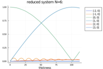
Figure 11: Beam amplitudes $|\psi_{g}(z)|$ of solutions for the three choices ${\mathbf{G}}_{1}$, ${\mathbf{G}}_{2}$, and ${\mathbf{G}}_{3}$. The same beating of the two main modes is observed in all the cases.

From Figure 11 we have a first qualitative comparison for the systematic-row cases. We see that the qualitative features, meaning the beating and the two main modes, namely $(0,0)$ and $(1,0)$, are captured in every case. The two beam case however fails to capture the other two main modes, for $(-1,0)$ and $(2,0)$.

To obtain a quantitative comparison of the different models we show the numerical values of $\psi_{(1,0)}(z_{*})$ and $\psi_{(2,0)}(z_{*})$ in Figure 12. As a first observation we see that the two-beam case has only one significant digit correct, making it a very rough approximation. Similar limitations of the two-beam approximation were observed in [19, 26] when doing simulations with CUFOUR.

Moving to ${\mathbf{G}}_{2}$ with four beams gives an accuracy of 4 significant digits, while increasing the size of the systematic-row approximation further does not bring higher accuracy as ${\mathbf{G}}_{3}$ with six beams still has only four significant digits. The accuracy of the solutions can only be improved by going beyond the systematic-row approximation (see Section 4.4). Indeed, we obtain 7 significant digits by adding the layer above and below the Ewald sphere in the ${\mathbf{G}}_{4}$ system, which has 18 beams.

​System​ $(0,0)$ mode $(1,0)$ mode ​digits​ ${\mathbf{G}}_{1}$ $-\underline{0.16}153606468-\underline{0.07}740830300\,\mathrm{i}$ $\underline{0.4}2515771142-\underline{0.8}8721717658\,\mathrm{i}$ 1 ${\mathbf{G}}_{2}$ $-\underline{0.1644}6909478-\underline{0.0676}6454587\,\mathrm{i}$ $\underline{0.3779}0257701-\underline{0.9077}5029000\,\mathrm{i}$ 4 ${\mathbf{G}}_{3}$ $-\underline{0.1644}5260546-\underline{0.067648}75833\,\mathrm{i}$ $\underline{0.377}89496977-\underline{0.9077}5362575\,\mathrm{i}$ 4 ${\mathbf{G}}_{4}$ $-\underline{0.1644425}2690-\underline{0.0676480}8597\,\mathrm{i}$ $\underline{0.3779141}0830-\underline{0.9077468}3865\,\mathrm{i}$ 7 ${\mathbf{G}}$ $-0.16444251537-0.06764807576\,\mathrm{i}$ $0.37791412093-0.90774682391\,\mathrm{i}$ —

Figure 12: Comparison of solutions for $\tilde{g}=(0,0)$ and $\tilde{g}=(1,0)$. The underlined decimals indicate which numbers are already correct (up to rounding) with respect to the last line, i.e. we take the ${\mathbf{G}}$ system as reference.

For comparing numerical errors with the mathematical error bounds in Figure 8, we observe that the scattering length is $\ell_{\mathrm{scatt}}=\frac{|k_{0}|}{|C_{U}|}=60.83\,\mathrm{nm}\approx z_{*}/2$. Choosing $\alpha_{*}=a_{0}=0.565\,\mathrm{nm}$ and using $|k_{0}|=0.608\cdot 10^{12}\,\mathrm{m}^{-1}$, we find the error terms

$$|\alpha_{*}k_{0}|^{-2}=0.0000084647989\lll 1\quad\text{and}\quad\frac{\alpha_{*}z_{*}}{\ell_{\mathrm{scatt}}^{2}}=0.01735570\ll 1,\vspace*{-0.2em}$$

which are indeed small for the chosen setup.

For many practical purposes, like the simulation of TEM images with pyTEM as in [15] (see Figure 2) an accuracy of 4 significant digits is certainly good enough. However, for other applications higher accuracy may be needed, e.g. for detecting phase differences for beams of low amplitudes like in electron holography, see e.g. [11].

In fact, the software pyTEM creates a beam list ${\mathbf{G}}$ in the following way. It first restricts to the LOLZ or systematic-row approximation by setting $g_{z}=0$. Next, a minimum for $|U_{g}|$ is chosen to restrict to the sublattice generated by those $g$ with $|U_{g}|\geq u_{\text{min}}$. For instance, the coefficients displayed in Figure 5(b) lead to the sublattice $\big{\{}\,g=\frac{1}{a_{0}}(0,2m,0)\>\big{|}\>m\in{\mathbb{Z}}\,\big{\}}$. Finally, a maximum value $\widetilde{s}_{*}$ is chosen for the excitation error $s_{g}$, which leads to a final systematic row approximation with 12 beams with $m\in\{-5,\ldots,6\}$. Thus, it covers the same range as our set ${\mathbf{G}}_{3}$.

Acknowledgments.

This research has been partially funded by Deutsche Forschungsgemeinschaft (DFG) through the Berlin Mathematics Research Center MATH+ (EXC-2046/1, project ID: 390685689) via the Berlin Mathematical School, the project EF3-1: Model-based geometry reconstruction from TEM images, and the project AA2-5 Data-driven electronic-structure calculations for nanostructures. The authors are grateful to Tore Niermann, TU Berlin, for helpful and stimulating discussions.

References

- [1] D. Benedetto, R. Esposito, and M. Pulvirenti, Asymptotic analysis of quantum scattering under mesoscopic scaling, Asympt. Analysis, 40 (2004), pp. 163–187.
- [2] C. G. Darwin, The theory of X-ray reflexion. Part I and II, Phil. Mag., 27 (1914), pp. 315–333 and 675–690.
- [3] M. De Graf, Introduction to Conventional Transmission Electron Microscopy, Cambridge University Press, 2003.
- [4] P. P. Ewald, Die Berechnung optischer und elektrostatischer Gitterpotentiale, Annalen der Physik, 3 (1921), pp. 253–287.
- [5] F. Hövermann, H. Spohn, and S. Teufel, Semiclassical limit for the Schrödinger equation with a short scale periodic potential, Commun. Math. Physics, 215 (2001), pp. 609–629.
- [6] A. Howie and M. J. Whelan, Diffraction contrast of electron microscope images of crystal lattice defects. ii. The development of a dynamical theory, Proc. Royal Soc. London Ser. A, 263 (1961), pp. 217–237.
- [7] R. James, Applications of perturbation theory in high energy electron diffraction, PhD thesis, University of Bath, 1990.
- [8] E. Javon, A. Lubk, R. Cours, S. Reboh, N. Cherkashin, F. Houdellier, C. Gatel, and M. J. Hÿtch, Dynamical effects in strain measurements by dark-field electron holography, Ultramicroscopy, 147 (2014), pp. 70–85.
- [9] S. Jin, P. Markowich, and C. Sparber, Mathematical and computational methods for semiclassical Schrödinger equations, Acta Numerica, (2011), pp. 121–209.
- [10] E. J. Kirkland, Advanced Computing in Electron Microscopy, Springer, 3rd ed., 2020.
- [11] H. Lichte, Electron holography: phases matter, Microscopy, 62 (2013), pp. S17–S28.
- [12] A. Lubk, E. Javon, N. Cherkashin, S. Reboh, C. Gatel, and M. Hÿtch, Dynamic scattering theory for dark-field electron holography of 3D strain fields, Ultramicroscopy, 136 (2014), pp. 42–49.
- [13] L. Meißner, T. Niermann, D. Berger, and M. Lehmann, Dynamical diffraction effects on the geometric phase of inhomogeneous strain fields, Ultramicroscopy, 207 (2019), p. 112844.
- [14] A. Maltsi, T. Niermann, T. Streckenbach, K. Tabelow, and T. Koprucki, Numerical simulation of tem images for in(ga)as/gaas quantum dots with various shapes, Opt. Quantum Electr., 52 (2020), pp. 1–11.
- [15] T. Niermann, pyTEM: A python-based TEM image simulation toolkit. Software, 2019.
- [16] E. Pascal, Dynamical models for novel diffraction techniques in SEM, PhD thesis, University of Strathclyde, 2019.
- [17] E. Pascal, B. Hourahine, G. Naresh-Kumar, K. Mingard, and C. Trager-Cowan, Dislocation contrast in electron channelling contrast images as projections of strain-like components, Materials Today: Proceedings, 5 (2018), pp. 14652–14661.
- [18] E. Pascal, S. Singh, P. G. Callahan, B. Hourahine, C. Trager-Cowan, and M. De Graef, Energy-weighted dynamical scattering simulations of electron diffraction modalities in the scanning electron microscope, Ultramicroscopy, 187 (2018), pp. 98–106.
- [19] R. Schäublin and P. Stadelmann, A method for simulating electron microscope dislocation images, Mater. Sci. Engin., A164 (1993), pp. 373–378.
- [20] M. Schowalter, A. Rosenauer, J. Titantah, and D. Lamoen, Computation and parametrization of the temperature dependence of Debye–Waller factors for group IV, III–V and II–VI semiconductors, Acta Crystall. A, 65 (2009), pp. 5–17.
- [21] D. van Dyck, The importance of backscattering in high-energy electron diffraction calculation, phys. stat. sol. (b), 77 (1976), pp. 301–308.
- [22] B. Viguier, M. Martinez, and J. Lacaze, Characterization of complex planar faults in FeAl(B) alloys, Intermetallics, 83 (2017), pp. 64–69.
- [23] A. Wang and M. De Graef, Modeling dynamical electron scattering with Bethe potentials and the scattering matrix, Ultramicroscopy, 160 (2016), pp. 35–43.
- [24] A. L. Weickenmeier and H. Kohl, Computation of absorptive form factors for high-energy electron diffraction, Acta Crystall. A, 47 (1991), pp. 590–597.
- [25] A. Winkelmann, C. Trager-Cowan, F. Sweeney, A. P. Day, and P. Peter, Many-beam dynamical simulation of electron backscatter diffraction patterns, Ultramicroscopy, 107 (2007), pp. 414–421.
- [26] W. Wu and R. Schaeublin, TEM diffraction contrast images simulation of dislocations, J. Microscopy, 275 (2019), pp. 11–23.
- [27] C. Zhu and M. De Graef, EBSD pattern simulations for an interaction volume containing lattice defects, Ultramicroscopy, 218 (2020), pp. 113088/1–12.