Lycoris - a large-area, high resolution beam telescope

Abstract

A high-resolution beam telescope is one of the most important and demanding infrastructure components at any test beam facility. Its main purpose is to provide reference particle tracks from the incoming test beam particles to the test beam users, which allows measurement of the performance of the device-under-test (DUT). Lycoris, a six-plane compact beam telescope with an active area of $\sim$10$\times$$10\text{\,}{\mathrm{cm}}^{2}$ (extensible to 10$\times$$20\text{\,}{\mathrm{cm}}^{2}$) was installed at the DESY II Test Beam Facility in 2019, to provide a precise momentum measurement in a $1\text{\,}\mathrm{T}$ solenoid magnet or to provide tracking over a large area.

The overall design of Lycoris will be described as well as the performance of the chosen silicon sensor. The $25\text{\,}\mathrm{\SIUnitSymbolMicro m}$ pitch micro-strip sensor used for Lycoris was originally designed for the SiD detector concept for the International Linear Collider. It adopts a second metallization layer to route signals from strips to the bump-bonded KPiX ASIC and uses a wire-bonded flex cable for the connection to the DAQ and the power supply system. This arrangement eliminates the need for a dedicated hybrid PCB. Its performance was tested for the first time in this project. The system has been evaluated at the DESY II Test Beam Facility in several test-beam campaigns and has demonstrated an average single-point resolution of $7.07\text{\,}\mathrm{\SIUnitSymbolMicro m}$.

1 Introduction

Beam telescopes have become the workhorse for many campaigns at test beam facilities. Typically, they consist of two stations or arms, each made up of a set of tracking sensors with a configurable spacing in between, where the Device-under-test (DUT) is usually placed. They provide very precise reference tracks and may also provide a common trigger, DAQ integration and even common reconstruction packages.

For over a decade, EUDET-style pixel beam telescopes [1] have been a success-story with a wide-ranging user community and strongly supported by the EU-funded EUDET [2], AIDA [3] and AIDA-2020 [4] projects. EUDET-style telescopes have six planes of Mimosa26 [5, 6] monolithic active pixel sensors providing high-precision beam tracking of around $2\text{\,}\mathrm{\SIUnitSymbolMicro m}$ in a small active area of 2$\times$$1\text{\,}{\mathrm{cm}}^{2}$. The telescope comes in a full package including a common trigger logic unit, the EUDET TLU [7], a DAQ framework called EUDAQ [8] allowing an easy integration of the user DAQ, and a complete reconstruction software suite called the EUTelescope package [9].

Seven copies of EUDET-style pixel beam telescopes have been made and are installed at CERN (PS and SPS), at the DESY II Test Beam Facility [10], ELSA in Bonn, and at ESTB [11] at SLAC. A large number of different user setups have been integrated into EUDAQ and benefited from the EUDET TLU [7] and used EUTelescope for the data reconstruction. The user community at the various test beam facilities has been very satisfied with the EUDET-style pixel beam telescopes but there were two requests which could not be met: having a telescope for large DUTs inside the PCMAG $1\text{\,}\mathrm{T}$ solenoid  [12] located at the DESY II Test Beam Facility and a large-area tracking coverage for e.g. calorimeter setups. The former is suffering from the fact that the EUDET-style telesopes have each sensor plane housed in a $1.5\text{\,}\mathrm{cm}$ thick aluminium case with a dedicated cooling pipe and an auxiliary board. While both the former and the later are limited by the small active area of the EUDET-style telescopes.

The design, construction and installation of a large active area, compact telescope at the DESY II Test Beam Facility became one of the deliverables [13] of AIDA-2020. This telescope, named Lycoris , was from the beginning based on six planes of silicon-strip sensors oriented in a small-angle-stereo configuration, to meet the desired coverage of at least 10$\times$$10\text{\,}{\mathrm{cm}}^{2}$.

Within AIDA-2020, there were strong activities on developing a successor of EUDET-TLU called the AIDA-TLU [14] and a successor of EUDAQ called EUDAQ2 [15]. AIDA-TLU distributes a common clock to all DUTs and timestamps the triggers, thus it enables time-stamp based event reconstruction and removes the readout bottlenecks. EUDAQ2 has upgraded significantly from EUDAQ with a lot extended protocols and synchronisation modes. Both upgrades altogether enable new data taking modes beyond the classical “trigger-busy” approach of the EUDET-TLU, where the system trigger rate has been limited by the device with the slowest readout, see details in [14]. All EUDET-style pixel telescopes have already upgraded to AIDA-TLU with EUDAQ2 or, are in the process of doing so. Hence it was decided for Lycoris to use EUDAQ2 and the AIDA-TLU right from the beginning.

This paper is organized as follows: first the design requirements and an overview of the telescope design is given, followed by a detailed description of the sensor plane, its components and the overall system (Section 2). Then the description of the DAQ and the on-line software (Section 3) and the performance of the Lycoris telescope (Section 4). Finally, there is a description of how to integrate a DUT (Section 5) followed by an overall summary (Section 6).

2 The Lycoris Telescope System

The design of Lycoris was driven by two different use-cases: providing a large-area coverage for test beam setups and providing precision tracking inside the PCMAG solenoid, where the Lycoris arms have to fit in the gap between the DUT and the inner wall of the PCMAG field cage. It was quickly concluded that the second use-case imposes much more stringent constraints and hence the requirements were derived from this use-case.

2.1 Overall Requirements

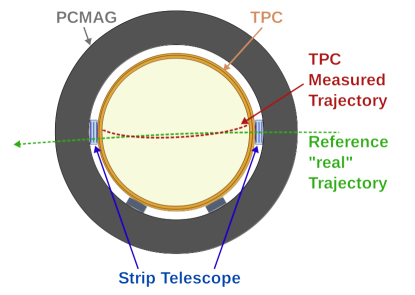
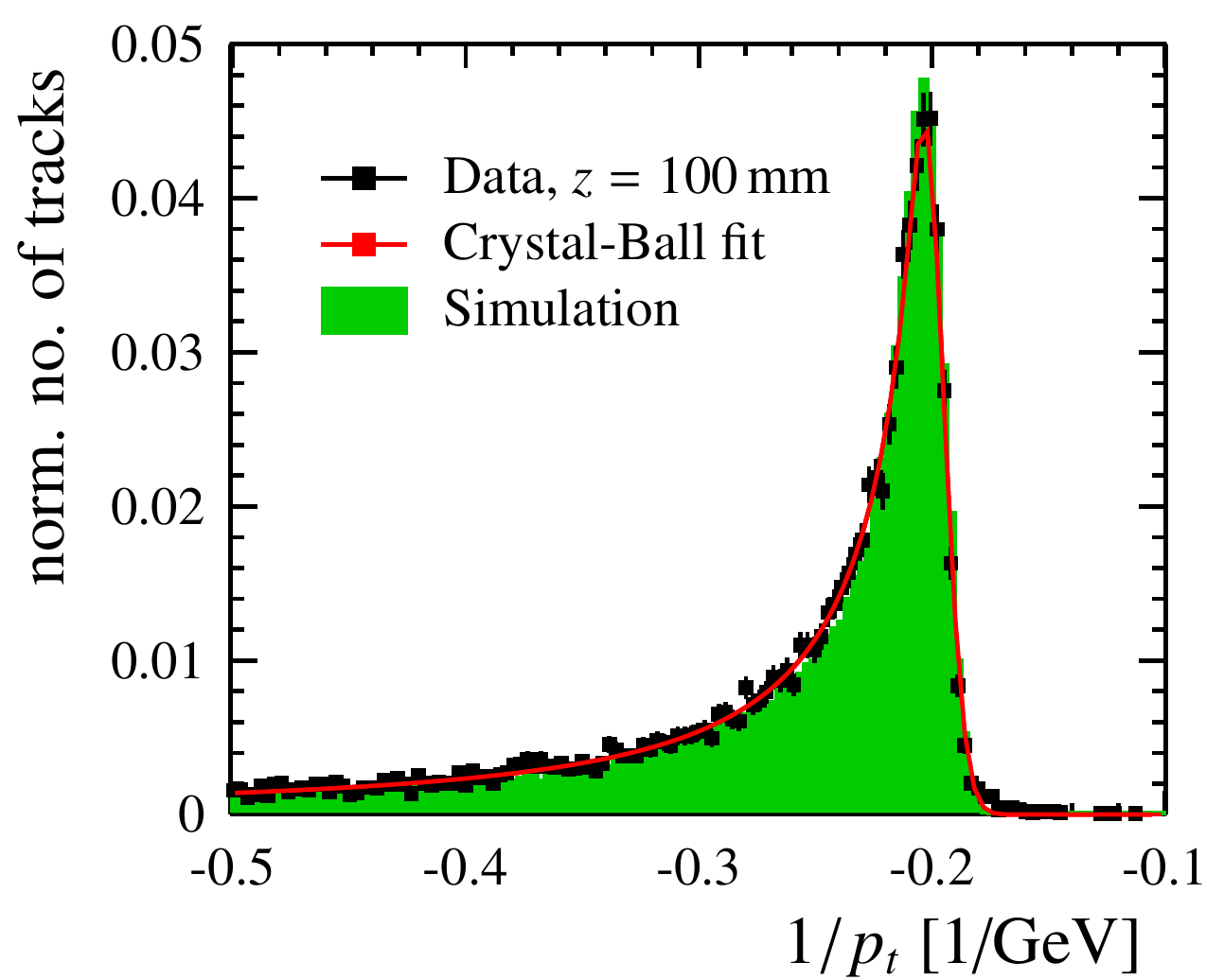
Figure 1: Picture of the PCMAG (left) [16] and the measured momentum spread (right) [17].

For tests in the PCMAG solenoid, the DUT (e.g. a Time Projection Chamber (TPC)) will be installed inside the PCMAG with a small gap on either side, where the Lycoris telescope will be installed. It will then be used to provide a precise measurement of the particle trajectory inside the magnet. As a result of interactions of the electrons with the magnet wall ($20\%$ radiation length $X_{0}$), the particles have a large momentum spread when entering the magnet volume (see Figure 1) compared to the momentum spread of the electron test beam itself. Effects such as poor momentum resolution due to potential electric field inhomogeneities within a TPC volume could be studied and corrected with precision information from Lycoris.

Simulation studies have been performed to determine the general requirements on such a system. A Geant4 [18, 19] simulation accurately describing the current infrastructure including the material and dimensions of the PCMAG and a TPC field cage (a detector taken as an example of one potential DUT) has been performed. These studies have shown that a spatial resolution of better than $10\text{\,}\mathrm{\SIUnitSymbolMicro m}$ is required in the bending plane of a homogeneous $1\text{\,}\mathrm{T}$ magnetic field, in order to provide a comparable momentum measurement to a TPC with resolution of $\sim$$5.0\text{\times}{10}^{-3}\text{\,}{\mathrm{GeV}}^{-1}$. The overall active area was required to be at least 10$\times$$10\text{\,}{\mathrm{cm}}^{2}$ in order to cover 96% of beam particles at $6\text{\,}\mathrm{GeV}$ according to the simulation results shown in Figure 2.

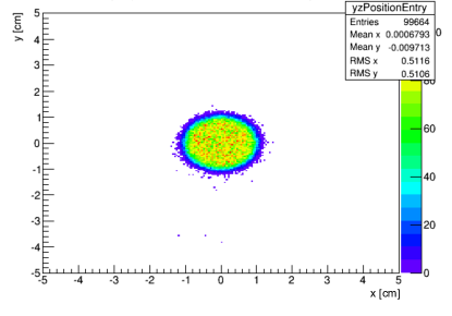
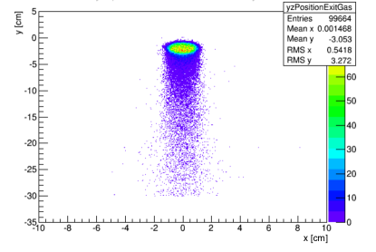
Figure 2: Simulated spread of $6\text{\,}\mathrm{GeV}$ beam at the silicon sensor plane before the TPC field cage (left) and at the last sensor plane (right). The coordination origin of the simulation is set to be the center of the PCMAG geometrical center. The beam spot is centered at $z=$ $2\text{\,}\mathrm{m}$ with radius of $0.5\text{\,}\mathrm{mm}$ and a spread of $2\text{\,}\mathrm{mrad}$, in order to well describe the beam status with a $1\text{\,}\mathrm{mm}$ diameter collimator at DESY II Test Beam Facility.

Two technology candidates – silicon-strip sensors and silicon-pixel sensors – have been considered. While the level of 3D information for a pixel system was superior, the available pixel sensors could not meet the area requirements at an affordable cost. Thus silicon-strip sensors with a sufficiently small pitch were chosen for this project. To provide the required 3D point resolution information, six silicon-strip sensors with a small-angle stereo configuration are used. The limiting factor guiding these choices is the available gap, which is as little as $3.5\text{\,}\mathrm{cm}$ and therefore provides a rather small lever arm. From these studies, it was decided to build a telescope with six layers in two stations of three sensors each and foresee configurations with 10$\times$$10\text{\,}{\mathrm{cm}}^{2}$ and 10$\times$$20\text{\,}{\mathrm{cm}}^{2}$ coverage, requiring six or twelve sensors in total. The key design requirements are summarized in Table 1.

Resolution in bending plane	$\sigma_{y}$	$<$ $10\text{\,}\mathrm{\SIUnitSymbolMicro m}$
Resolution orthogonal to the bending plane	$\sigma_{x}$	$<$ $1\text{\,}\mathrm{mm}$
Area coverage	$A_{xy}$	10$\times$ $10\text{\,}{\mathrm{cm}}^{2}$
Thickness of single station	d	$<$ $3.5\text{\,}\mathrm{cm}$

Table 1: The key design requirements for developing the Lycoris telescope.

Moreover, this design also meets the need to operate the telescope outside of the PCMAG, where several user groups have indicated their interest to make use of the large area coverage provided by Lycoris, e.g. from the CALICE Collaboration.

2.2 Overall Telescope Design

The resolution requirements described above imply a strip pitch of about $25\text{\,}\mathrm{\SIUnitSymbolMicro m}$ or smaller. Most silicon-strip sensors used in particle physics or nuclear physics experiments do not provide the required spatial resolution and/or the area coverage requirements for this telescope. For example, silicon-strip sensors developed for the HL-LHC mainly use a pitch of $\approx$ $75\text{\,}\mathrm{\SIUnitSymbolMicro m}$ [20, 21]. The silicon-strip sensor designed for the main tracker of the SiD detector [22, 23] for the ILC [24] was found to have the needed properties and was chosen for Lycoris.

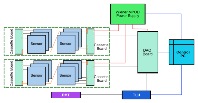
Figure 3: The overall design of the Lycoris telescope. The cassettes are indicated by the green dashes and host up to six sensor modules and two cassette boards. The High Voltage(HV)/Low Voltage(LV) connections are indicated in red, while the connections for the DAQ are indicated in dark grey, the Ethernet connections using TCP/IP in blue and the connections using the Kapton-flex in orange.

The overall architecture of Lycoris is shown in Figure 3. The two separate stations are called “cassettes” and provide the mechanical support for up to six sensor planes in total. Three sensor units – the modules – are controlled by one cassette board, which acts as the interface to the power supply crate (Wiener MPOD) and the DAQ using the SLAC KPiX DAQ board. The cassette board can be daisy-chained to a secondary cassette board to control six sensor planes. The DAQ board supports up to four cassette boards and interfaces with a control PC via Ethernet and with the AIDA-TLU [14] via an HDMI connector. Triggering is provided by a coincidence from a set of scintillators  read out by photo-multiplier tubes (PMT). The individual telescope components are described in detail in Section 2.3.

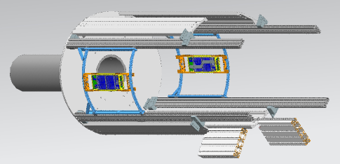
Figure 4: CAD drawing of the mechanical support to integrate Lycoris telescope inside the PCMAG, where the rails marked in light-blue are used by the two Lycoris cassettes.

The most stringent mechanical requirements are due to operating Lycoris inside the PCMAG solenoid. The available gap between the current TPC and inner wall of the PCMAG allows merely a cassette thickness of $3.5\text{\,}\mathrm{cm}$. The PCMAG provides a rail system to install a DUT, so it can be moved in and out with high accuracy. The cassettes are mounted on a separate rail system, so they can slide in and out independently of the DUT itself. This simplifies both installation and operation. A CAD drawing of the actual setup is shown in Figure 4.

2.3 The Lycoris Silicon Sensor Module

The central building block of Lycoris is the silicon sensor module shown in Figure 5 which is composed of one SiD tracker sensor, two KPiX ASICs [25] and a Kapton-flex cable. As the KPiX ASICs are bump-bonded directly on top of the silicon-sensor, there is no need for a hybrid PCB.

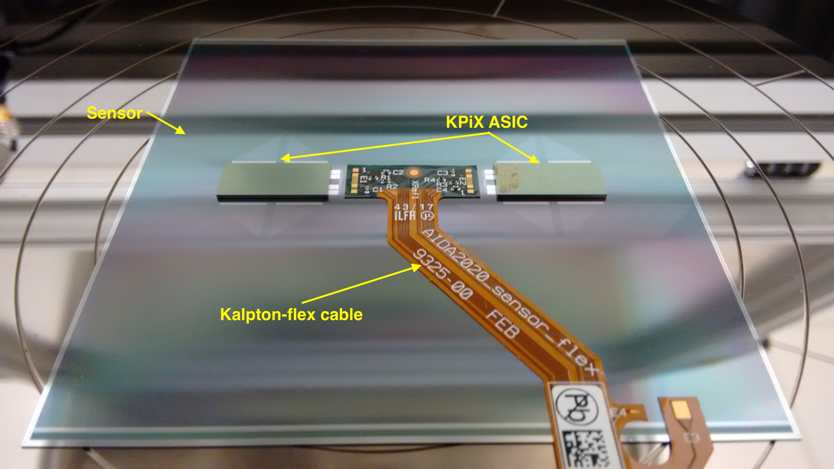
Figure 5: The Lycoris module composed of one SiD tracker sensor, two KPiX ASICs and a Kapton-flex readout cable.

2.3.1 The SiD Tracker Sensor

The sensor designed for the SiD tracker, called SiD-OUTER-SSSD 6972, is an n-type silicon micro-strip sensor with $25\text{\,}\mathrm{\SIUnitSymbolMicro m}$ pitch (read out on every other strip) manufactured by Hamamatsu [26]. It provides a spatial resolution of $\sim$$7.2\text{\,}\mathrm{\SIUnitSymbolMicro m}$ . The sensor is designed with two aluminum metallization layers, as shown in the schematic cross-section in Figure 6, which enables the hybrid-less design. Table 2 gives the detailed properties of this sensor.

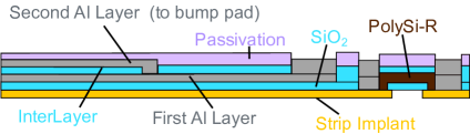
Figure 6: Schematic cross-section of the SiD tracker sensor.

The second metallization layer routes signals of each strip to a bump pad that is bonded directly to the KPiX readout ASIC. This layer is also used for powering the KPiX ASIC and transmitting other digital signals such as Command, Clock and Trigger. This approach to a hybrid-less strip sensor design has been tested for the first-time in this project.

	SiD-OUTER-SSSD 6972
Sensor size	$93.53\times$$93.53\text{\,}{\mathrm{mm}}^{2}$
Thickness	320$\pm$$15\text{\,}\mathrm{\SIUnitSymbolMicro m}$
Crystal Orientation	<100>
Wafer type	n-type
Strip implant	p+ type
Strip p+ width	$8\text{\,}\mathrm{\SIUnitSymbolMicro m}$
Strip Al width	$9\text{\,}\mathrm{\SIUnitSymbolMicro m}$
Readout Al width	$4\text{\,}\mathrm{\SIUnitSymbolMicro m}$
Strip bias resistance	10-$50\text{\,}\mathrm{M\SIUnitSymbolOhm}$/strip
Strip readout coupling	AC
Strip Pitch (readout)	$25\text{\,}\mathrm{\SIUnitSymbolMicro m}$ ($50\text{\,}\mathrm{\SIUnitSymbolMicro m}$)
Strip Multiplicity (readout)	3679 (1840)

Table 2: The SiD tracker sensor (SiD-OUTER-SSSD 6972) properties.

2.3.2 The KPiX ASIC

The KPiX readout chip was designed by SLAC as a multi-purpose read-out ASIC for the SiD detector concept for the ILC. It was manufactured using a $250\text{\,}\mathrm{nm}$ mixed-mode CMOS process from TSMC [27]. The chip consists of a 1024 channel fully digital readout with a 13-bit ADC and a timing generator controlling the data acquisition. Each channel consists of a charge amplifier, a shaper and a discriminator. The charge amplifier can be operated either in a high-gain or low-gain mode and additionally offers a dynamically switchable gain range. If the default range of $400\text{\,}\mathrm{fC}$ has been exceeded, which is detected in the range control circuitry, a $10\text{\,}\mathrm{pF}$ capacitor is automatically added to extend the range to $10\text{\,}\mathrm{pC}$. For a bare KPiX, the noise floor is about 1000 electrons in the low-gain mode and 700 electrons for the high-gain mode For a full assembled sensor, a noise floor of 5% of a Minimum Ionizing Particle (MIP) in the $320\text{\,}\mu\mathrm{m}$ thick silicon tracker sensor was achieved. The dynamic range switching then extends the available range to 2500 MIPs.

Figure 7 shows the block diagram of a single KPiX readout channel. Each channel has four sample and hold capacitors and four timing registers to permit four separate measurements of the signal amplitude and the time of threshold crossing. This results in four memory buckets for each channel. In normal operation, the charge amplifier is synchronously reset after each bunch-crossing.

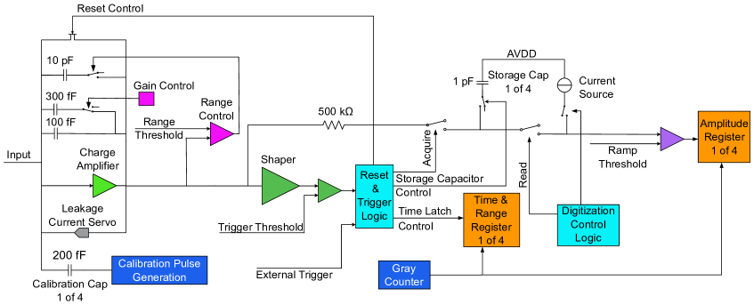
Figure 7: Simplified block diagram of a single KPiX readout channel (out of 1024 channels in total). Shown are the charge-amplifier in light green with its gain control and dynamic range-control circuitry (shown in pink) and the shaper (green). The main digital blocks are indicated in light and dark blue with the memory buckets shown in orange.

Each channel has a calibration system, leakage compensation, “DC” reset and polarity inversion. KPiX supports both AC and DC-coupled signals and in DC mode the leakage is compensated by a servo circuit. The total amount of leakage is determined without any signal being present during the data taking period. The “DC” reset works for asynchronous operation for cosmic-ray runs. KPiX can switch the input polarity for use with e.g. GEM detectors [28, 29]. The noise floor is about 1000 electrons in low-gain mode ($0.15\text{\,}\mathrm{fC}$) and the maximum signal charge is $10\text{\,}\mathrm{pC}$ with the full dynamic range corresponding to 17 bits. KPiX uses two separate power supply lines for its analog (AVDD) and digital (DVDD) circuits, requiring nominally $2.5\text{\,}\mathrm{V}$ and $2.0\text{\,}\mathrm{V}$ respectively. KPiX has been designed to achieve an average power consumption lower than $20\text{\,}\mu\mathrm{W}\mathrm{/}\mathrm{c}\mathrm{h}\mathrm{a}\mathrm{n}\mathrm{n}\mathrm{e}\mathrm{l}$ for applications at the ILC realized by power-pulsing. This is realized by powering the analog front end only when beam is present, i.e. during the signal acquisition period. This power-pulsing cycle is called the KPiX data acquisition cycle. It starts with an external Acquisition Start Signal followed by five different operational states and a shut-off idle phase. The sequence of the five states and the idle phase is shown in Figure 8.

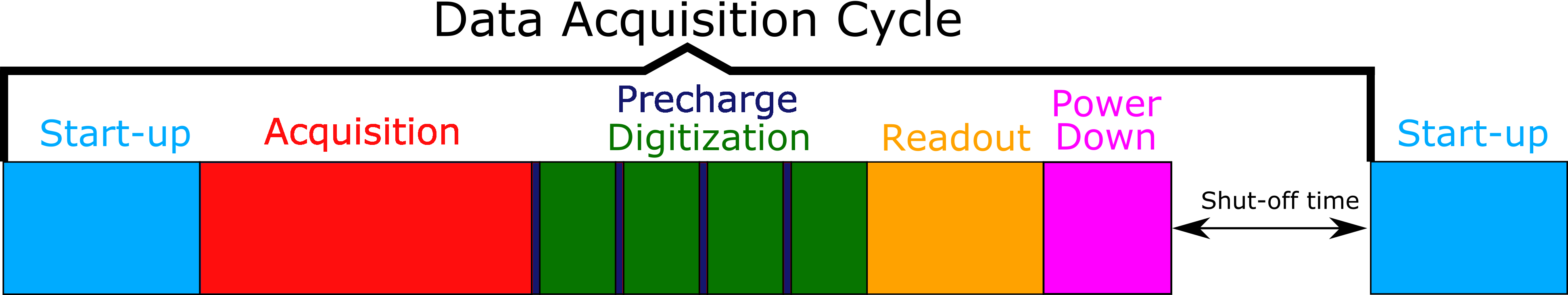
Figure 8: The five operational states of KPiX data acquisition cycle followed by the between beam bunches shut-off idle phase (relative time periods for states not to scale).

An externally provided DAQ board is able to adjust the period of the KPiX clock separately for each state, in $5\text{\,}\mathrm{ns}$ increments with a minimum period of $10\text{\,}\mathrm{ns}$. This allows a wider acquisition and pre-charge window to be achieved, while at the same time reducing the time spent on digitization and readout. Table 3 shows the typical clock periods to operate KPiX at each state, including the five data acquisition operational states and the shut-off idle phase. These unique properties of the KPiX ASIC make it ideal for the ILC environment. In addition to its use in the SiD tracking system, as discussed in Section 2.3.1, KPiX is also the proposed readout strategy for the SiD Silicon-tungsten sampling electromagnetic calorimeter [30, 31], as the many readout channels read out between beam bunch crossings through a power-pulsing cycle allow for a highly granular and compact calorimeter design with a minimal cooling system.

Clock	Typical clock period (ns)
$T_{\mathrm{Acquisition}}$	320
$T_{\mathrm{Digitization}}$	50
$T_{\mathrm{Pre-Charge}}$	6000
$T_{\mathrm{Readout}}$	200
$T_{\mathrm{Idle}}$	200

Table 3: The KPiX clock domains and the typical clock periods to operate KPiX at each state.

The five operational states of the KPiX data acquisition cycle (shown in Figure 8) are described in the following.

Start-up:

KPiX powers up after receiving the Acquisition Start Signal. The start up phase duration is configurable via the TimeBunchClkDelay setting and during this phase the KPiX uses the acquisition clock $T_{\mathrm{Acquisition}}$. KPiX operation during this phase includes the ramp up of analog and digital current to operation values and the resetting of internal KPiX registers and the Gray counter.

$$t_{\mathrm{Start-up}}=T_{\mathrm{Acquisition}}\cdot TimeBunchClkDelay$$

Acquisition:

The acquisition phase is the period when the chip records data and the clock used is the acquisition clock $T_{\mathrm{Acquisition}}$. During this phase, the chip is able to store per channel up to four events in the analog buffers and timestamp each event using a 13-bit counter called BunchClockCount (BCC) which increments by every eight clock pulses and is cleared every cycle. The opening time for this phase $t_{\mathrm{acquisition}}$ is configurable by setting the maximum BCC ($n_{BCC,max.}$) thus calculated as

$$t_{\mathrm{Acquisition}}=n_{BCC,max.}\cdot 1\;BCC=n_{BCC,max.}\cdot 8\;T_{\mathrm{Acquisition}}\,\,.$$

There is a small configurable pause between readout and digitization which is used to prepare the analog buffers for the upcoming digitization.

Digitization:

The analog information stored in four storage capacitors for each of the 1024 channels is now digitized in four cycles, doing 1024 analog buckets in parallel. The digitization is handled by a Wilkinson ADC with a 13-bit resolution for each channel. A current mirrored into each of the 1024 channels runs down the charge in the storage capacitor for each cycle. The duration of the so-called pre-charge period is $2\cdot$ $T_{\mathrm{Pre-Charge}}$ per individual storage capacitor or $8\cdot$$T_{\mathrm{Pre-Charge}}$ in total. During the pre-charge the analog bus connecting the storage capacitors to the Wilkinson converters is charged to a known level as it can contain charge from a previous event as such it has to be done before connecting to the next storage capacitor. In addition, the read-out bus is pre-charged to high as the read-out can only pull the bus low. A ramp-threshold discriminator then detects the transition through zero, and the content of a common Gray counter is then stored in the corresponding memory bucket together with the corresponding timestamp determined by BCC and the range identifier bits. The total time required for the digitization of a single bucket, excluding the time for the pre-charge is

$$t_{\mathrm{Single-Digitization}}=(8192+18)\cdot T_{\mathrm{Digitization}}$$

with the total digitization time being given by

$$t_{\mathrm{Digitization}}=4\cdot(8192+18)\cdot T_{\mathrm{Digitization}}\,\,.$$

Readout:

After digitization is complete, all data is sequentially read out using the $T_{\mathrm{Readout}}$ clock. A KPiX word corresponds to 13 bits, corresponding to the ADC resolution and the BCC. The readout is organized in rows of 32 channels, which corresponds to 416 bits equivalent to $416\cdot$$T_{\mathrm{Readout}}$. Reading out each shift register is preceded by the parallel loading of all the shift registers which takes $300\cdot$$T_{\mathrm{Readout}}$. In total the readout of one row takes $716\cdot$ $T_{\mathrm{Readout}}$. For each channel there are nine words in total and KPiX has 32 rows of 32 channels in total.

Overall the entire readout of KPiX takes $32\cdot 9\cdot 716\cdot$$T_{\mathrm{Readout}}$ $=206208\cdot$$T_{\mathrm{Readout}}$.

Power-down:

After the readout has completed, the current is pulsed down while maintaining the supply voltages.

Additional details on the various KPiX trigger modes, the calibration circuitry and the interconnects are given below.

KPiX Trigger Modes

KPiX can take data in two different operation modes, corresponding to two different triggering schemes:

Self triggering:

If the charge generated within a channel rises above a user defined threshold, it will be recorded by KPiX.

External triggering:

When an external trigger arrives, KPiX records the generated charge from all channels simultaneously.

In both modes a maximum of four triggers per channel can be stored by KPiX. Given the preferred beam telescope operation and the usual need of an external trigger by DUT setups, the KPiX external trigger mode is the preferred running mode for the Lycoris telescope.

Calibration

In order to calibrate the ADC response, each of the 1024 readout channels is equipped with a calibration module which injects a series of user defined calibration amplitudes through an 8-bit DAC for verifying the ADC response. The ADC has a linear response to the different calibration values and its slope is consequently used in the following studies to convert the raw ADC value to a charge in fC. The calibration data-taking is operated using the external triggering mode with a software-controlled start signal. All the four memory buckets for every channel can be calibrated individually to correct for potential pedestal and offset differences. The first calibration pulse can be selected for a high calibration range, so that the system can be tested up to the full-scale range of $10\text{\,}\mathrm{pC}$. For negative-polarity signals, an inverter is inserted after the charge amplifier so the polarity of the calibration signal is reversed as well.

Interconnects

KPiX has been designed to be bump-bonded to various Silicon sensors. The eutectic Sn-Pb bumps on a $200\times$$500\text{\,}\mathrm{\SIUnitSymbolMicro m}$ lattice are placed in wells on each KPiX pad. Figure 9 (left) shows a schematic diagram of the KPiX bump bonding array, where the center bump matrix (blue/red) provides connections to the KPiX readout channels while the two outermost columns (black/green) route the AVDD/DVDD power, the digital input signals including the clock, control, external trigger and the outgoing digital data stream. Two KPiX chips are necessary to read out the 1840 strips of one SiD tracker sensor, but only 920 (blue) out of the 1024 readout channels of a single KPiX are connected to a strip while the others (red) are bonded to the sensor bump pads and are left floating. The bump pads on each side of KPiX are designed with the same functionality. The SiD tracker sensor is designed to connect only one side (green) of the KPiX power/signal bump-pads, thereby the other side (black) is left open. Figure 9 (right) shows a microscope photo of the pads on the sensor surface for bump-bonding and wire-bonding, where the marginal bump-bonding pads to provide KPiX power and signals are routed to the wire-bonding pads via the second metallization layer.

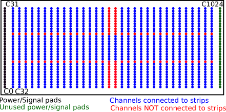
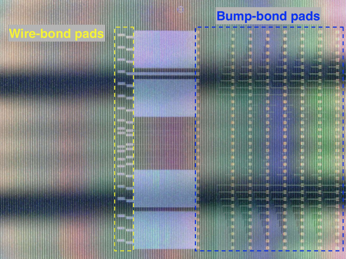
Figure 9: A schematic diagram of KPiX bump-bonding array (left) with the 920 connected channels in (blue). The two outermost columns (black/green) on each side route the AVDD/DVDD power to KPiX, as well as exchange digital signals. A microscope photo (right) of a section of the pad grid on the sensor surface. The bump-bonding pads (blue) connect to the used Power/Signal column (black on left sketch) of one KPiX and some of its neighboring pads. The wire-bonding pads (yellow) connect the Power/Signal column through the sensor’s second metallization layer to outside (via Kapton-Flex).

2.3.3 The Kapton-Flex Cable

The Kapton-Flex cable shown in Figure 10 is designed to route both HV and LV power and digital traces between the sensor module and the DAQ system. Both HV and LV lines are further filtered on the Kapton-Flex to further reduce the noise due to power supplies. It feeds the sensor bias voltage through wire-bonding from the HV bonding pad to the sensor bias ring, and the bias return is made by connecting the HV return to the sensor back plane using conductive silver epoxy paste. For the two KPiX chips on the same sensor, their low voltage traces (AVDD and DVDD) as well as their grounds, are tied together. For the same KPiX, the AGND and DGND are tied together through a $0\text{\,}\mathrm{\SIUnitSymbolOhm}$ resistor. The bias voltage is AC coupled to the KPiX AVDD through a bypass capacitor; KPiX is measuring through its analogue voltage instead of its analogue ground to avoid any mismeasurement from grounding differences. The clock and the trigger signals are Low Voltage Differential Signals (LVDS), of which the termination resistors are placed on this Kapton-Flex cable.

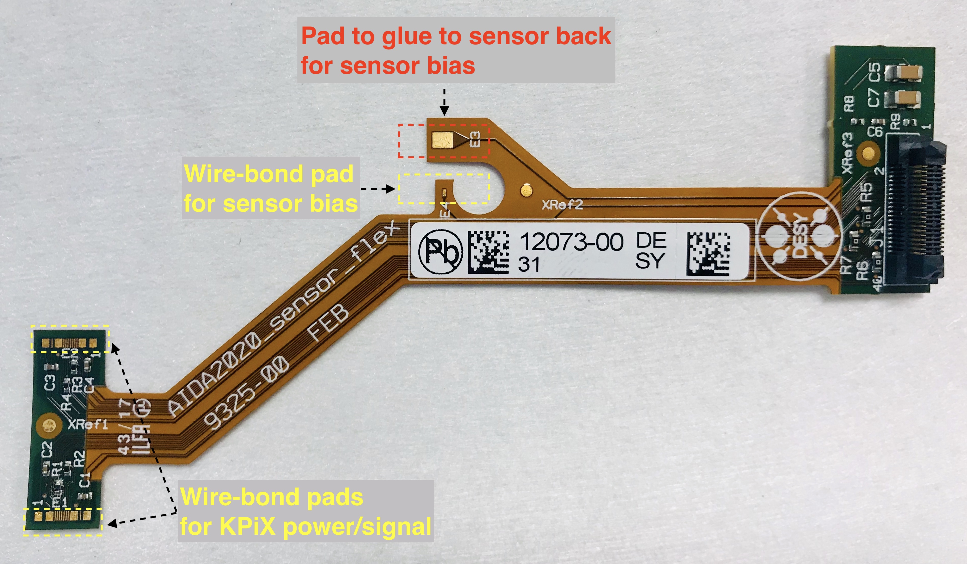
Figure 10: The Kapton-Flex cable used on the Lycoris module.

2.3.4 Module Assembly

Assembling a Lycoris module is a four-step process:

1. The bump-bonding between the two flipped KPiX chips and the silicon sensor;

2. Gluing the Kapton-Flex cable onto the silicon sensor;

3. Connecting the pads on Kapton-Flex cable with the corresponding pads on the silicon sensor using wire-bonding;

4. Silver epoxy glue the HV return pad on the Kapton-Flex cable to the sensor back plane.

Both bump-bonding and wire-bonding are well-established industry standard processes and have excellent track-records in assembling sensor modules for the LHC experiments. The bump-bonding were performed at Fraunhofer IZM. The bumps has been pre-applied on the KPiX by its manufacturer and the under bump metalization has also been pre-applied on the sensor by its manufacturer. The wire-bonding step were performed in-house at DESY. Placing a Kapton-Flex cable accurately on the active sensor surface using glue, however, is a highly customized process. Therefore, a dedicated gluing tool was designed to glue the Kapton-Flex to the sensor (see Figure 11). The non-conductive epoxy paste adhesive Araldite 2011 requiring 12 hours curing has been used based on the experiences of ATLAS [32] and the gluing procedure has been validated to ensure it meets the following requirements:

• No damage to the sensor when applying an even pressure on the glue area to obtain an optimal cure;

• The cable is positioned precisely to the area given by the edge of the three bonding areas and stays steady during the cure;

• No extra glue split over the wire-bonding pads which directly connects to the second metallization layer.

Among the 29 sensors produced, 24 have been successfully assembled, while two of them have not yet been fully assembled for future upgrades to the flex cable. The rest five sensors failed to be assembled for different reasons: one sensor was grinded down to validate the bump-bonding quality, two sensors failed to be wire-bonded due to aged bonding pads on the flex cable, and the rest two sensors were damaged by a high pressure during the gluing process. The quality of the 24 assembled sensor modules are further controlled by IV measurements. All the sensors show a typical development as shown in Section 4.4, except for two sensors that cannot deplete anymore .

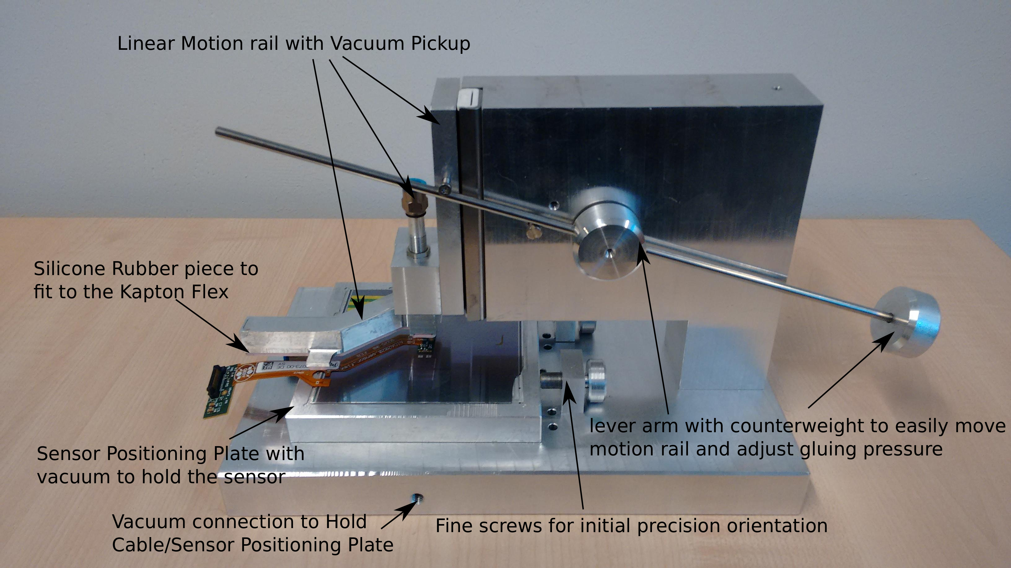
Figure 11: The custom gluing tool used to assemble the Lycoris modules.

2.4 The Cassette

The Lycoris cassette, which holds up to two stacks of three sensors, consists of an aluminum frame and two cassette boards and is covered by two carbon fiber windows as shown in Figure 12. The cassette is $3.3\text{\,}\mathrm{cm}$ tall, $12.1\text{\,}\mathrm{cm}$ wide and $32.1\text{\,}\mathrm{cm}$ deep. Each individual sensor module is glued to a frame which is designed together with the cassette so that the frame can be installed with three (+2, -2, 0 degree) different orientations. The frame is made out of Torlon, which is non-conductive but of similar strength as aluminum, so that it can be milled using standard techniques.

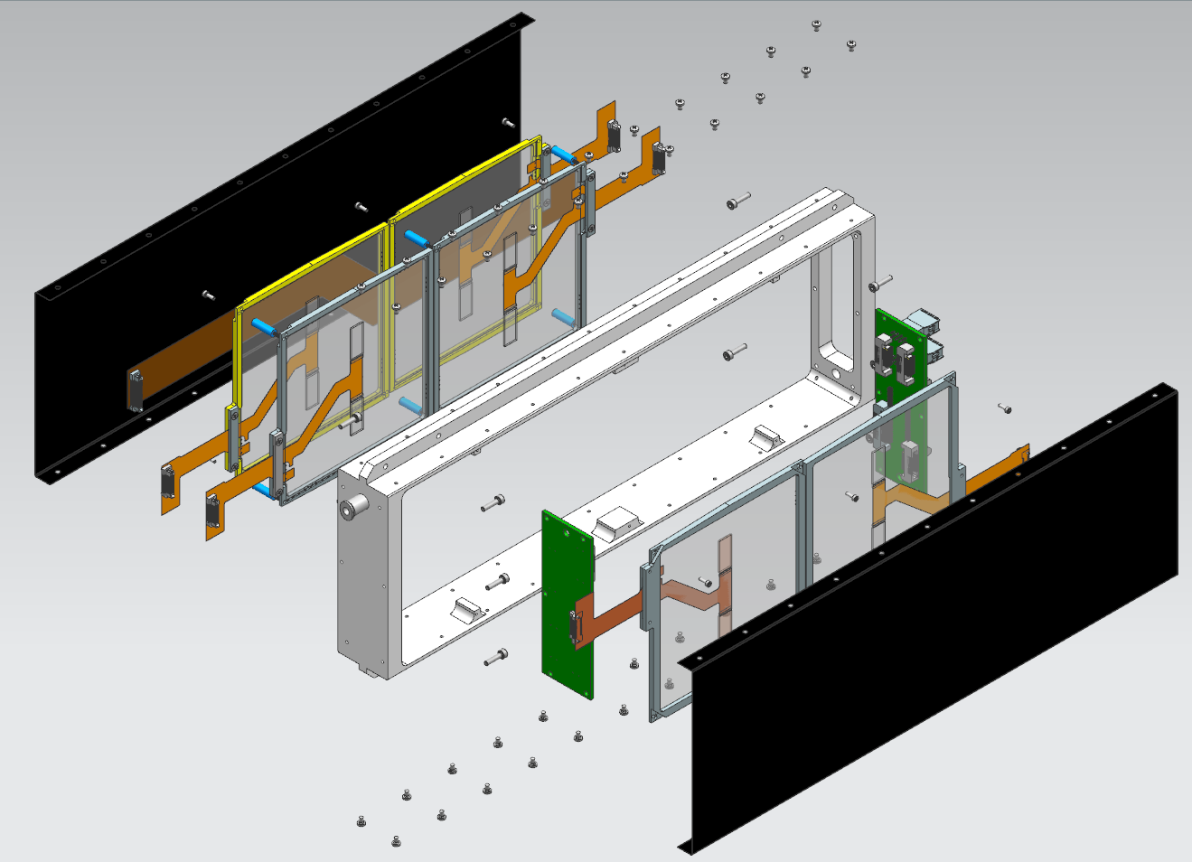
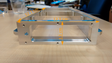
Figure 12: The Cassette: An exploded view of one Lycoris cassette holding two stacks of three sensors and two cassette boards (left) and a photo of the cassette frame with dimensions ($3.3\text{\,}\mathrm{cm}$ tall, $12.1\text{\,}\mathrm{cm}$ wide and $32.1\text{\,}\mathrm{cm}$ deep) (right).

2.4.1 The Cassette Board

The cassette board serves as a transition board between the DAQ board and the modules. It is designed to drive up to three sensor modules in a cassette. It distributes Low Voltage (LV) power to the connected KPiX chips through linear regulators with an input voltage of $3.0\text{\,}\mathrm{V}$, connects each High Voltage (HV) power line from the power supply to each connected sensor, and distributes all digital signals between the KPiX chips and the DAQ board. Each output line of the linear regulator is filtered separately for noise. AVDD (2.5V) is separately regulated for the two KPiX chips on the same sensor, while the digital power DVDD (2.0V) is shared by all KPiX ASICs from a single regulator.

Two versions of the cassette board exist and can be daisy-chained via a custom Kapton-Flex cable. One is installed at the front of the cassette and acts as the primary board while the other is installed at the other end of the cassette and serves as the secondary. They drive the connected sensor modules in the same way, but the primary cassette board has two extra functions. First, its outer side as shown in Figure 13 (left) hosts the interfaces with the DAQ board and the power supply for the sensors. Second, it has one I²C temperature and humidity sensor equipped on its inner side as shown in Figure 13 (middle) to monitor the environment inside the cassette.

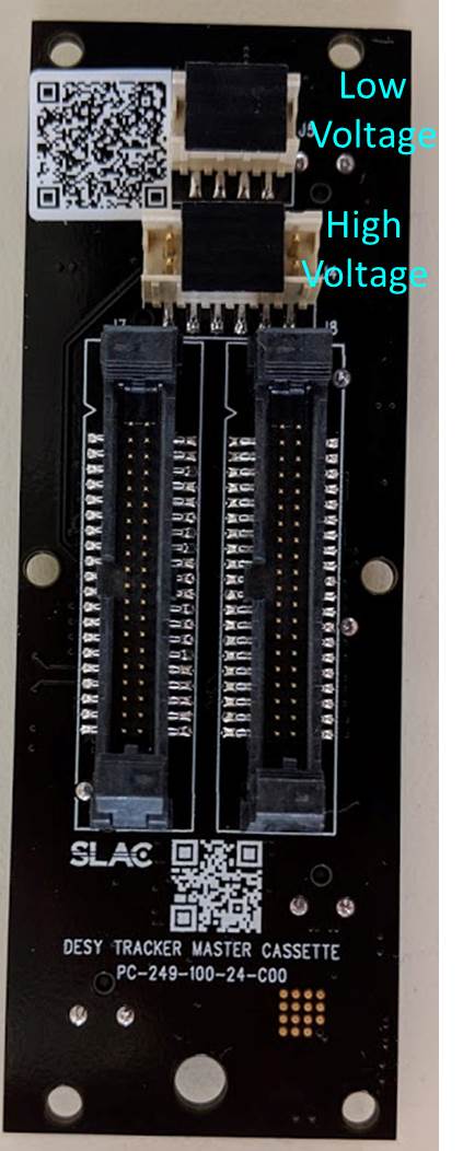
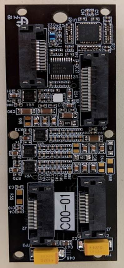
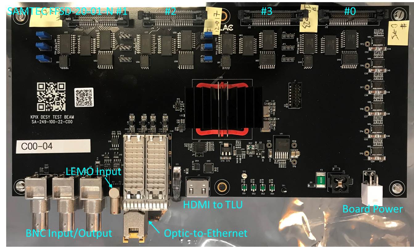
Figure 13: The primary cassette board (outer side - left and inner side - middle) and the DAQ board used by Lycoris (right).

2.5 Trigger and DAQ Hardware

The DAQ board used by Lycoris is shown in Figure 13 (right). It requires $12\text{\,}\mathrm{V}$ / $0.5\text{\,}\mathrm{A}$ for operation. It connects to the user control PC through an SFP port, allowing for flexibility in the physical interface used. Currently, the RJ-45 module is used for ease in connecting to standard 1000Base-T networking equipment, but it is possible to upgrade to optical Ethernet or a custom optical interface in the future if needed. The board is equipped with a Xilinx Kintex7 FPGA to provide I/O interfaces and event building. It has been designed with the following features:

• All signal interconnects with the connected cassette boards are communicated via isolation buffers, so that the DAQ board and all the connected KPiX chips are electrically isolated;

• Multiple input connections to provide acquisition start signals and external triggers for the KPiX data taking: two LEMO ports, two BNC ports and one HDMI port;

• An Ethernet interface using SFP+ plugins to connect to a PC running the DAQ software.

Lycoris is designed to synchronize with other devices using the AIDA-2020 Trigger Logic Unit (TLU). This has been implemented by correlating timestamps on triggers recorded respectively by Lycoris and by AIDA-2020 TLU. The DAQ board is able to record a global timestamp on each incoming trigger using a 64-bit counter which is incremented with every clock pulse of the $200\text{\,}\mathrm{MHz}$ FPGA system clock and is reset by an external start signal at the beginning of each data run. In order to correlate the Lycoris trigger timestamps to the TLU trigger timestamps, the DAQ board can use the $40\text{\,}\mathrm{MHz}$ TLU clock to generate its system clock and the 64-bit counter can be reset by the start signal $T_{0}$ sent out by the TLU. Both of the TLU clock and the $T_{0}$ signals are received through the HDMI input.

Besides the clock and the trigger signals, the TLU is also able to send out a so-called shutter signal to indicate the presence of the beam. This signal is generated with a configurable delay on the $E_{min}$ signal from the DESY II accelerator (see Section 4.2 for further details) and serves as the KPiX Acquisition Start Signal signal.

The latency of the trigger timestamps registered by Lycoris and by the TLU is important for the offline analysis in order to synchronize events between different devices. This latency has been measured and verified to be very stable for the same port of the same TLU unit. The variation among ports of different TLU units is very small resulting a typical latency of $105\text{\,}\mathrm{ns}$ .

2.5.1 DAQ Board FPGA Firmware

The FPGA firmware serves as a bridge between the DAQ software running on commodity PC hardware, and the interfaces required by the KPiX ASICs and the TLU timing system. The firmware allows for configuration and acquisition control of up to 24 attached KPiX chips. Configuration registers allow for acquisition to be driven by the TLU interface or a combination of DAQ software commands and TTL inputs. The later configuration is typically used for taking baseline and calibration data. Figure 14 shows the block diagram of the FPGA firmware. It reveals what is behind the digital traces between the DAQ board and the connected KPiX chips.

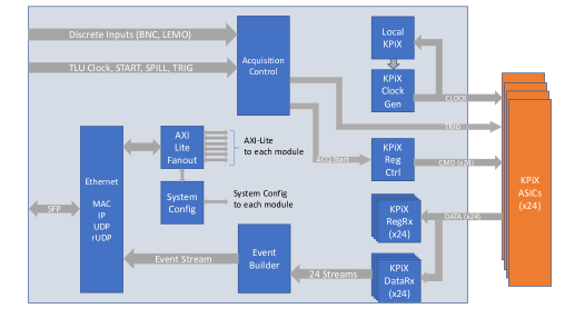
Figure 14: Block diagram of the DAQ firmware design.

The interface to the DAQ software consists of an Ethernet/IP/UDP stack, with an additional Reliable UDP (rUDP) layer on top to ensure reliable transmission of UDP packets. This entire stack actually accounts for over half of the firmware logic utilization of the design. The firmware uses an AXI-Lite bus internally for handling register transactions from software.

The KPiX ASIC digital interface consists of four signals: CLK, CMD, RSP, TRIG. Register read and write commands are sent serially on the CMD line. Register read responses arrive from the KPiX on the RSP line. Requests to start a new acquisition cycle are also sent on the CMD line, and the acquired data arrives serially on the RSP line once the acquisition is complete. Register access is not allowed during a KPiX acquisition. The firmware logic handles the serialization and deserialization of CMD and RSP, respectively. It also translates register access requests and acquisition start commands into the serial format expected by KPiX. During acquisition data readout, it reformats the serial data stream into 64-bit “samples", with each sample representing the ADC and timestamp data for a single channel/bucket in the system.

The firmware allows for the clock speed to change dynamically during each phase of the KPiX acquisition cycle. To accomplish this, the firmware runs a local copy of the KPiX digital logic, so that it can snoop on the current state of the KPiX. All KPiX chips in the system run in lockstep with each other, so the state of the local KPiX is the same as the chips on the sensors. The clock period to use during each phase is set via configuration registers prior to the start of each run.

For each acquisition, the Event Builder combines the 64-bit samples from each of the (up to) 24 attached KPiX ASICs into a single large data frame. Each KPiX has 1024 channels, and each channel has four buckets, so a data frame from an acquisition may contain up to 1024$\times$4$\times$24 samples. The data frame also contains a 4 $\times$ 64-bit word header containing timestamp and run count metadata.

2.6 Power Supplies

The power supply system used is a commercially available MPOD Mini system from Wiener which is mounted into a 19-inch rack. The WIENER LV MPV8016I provides all the LV (DAQ, AVDD and DVDD) and the one for HV is WIENER/ISEQ EHS F205x_106HV. This system can be remote-controlled via Ethernet using the SNMP protocol, thus providing online monitoring of the current and the voltage of each power line.

The power supply LV lines for the sensors in a cassette are common. They connect to a set of linear regulators on the cassette board and are then distributed to the sensors. Two LV lines serve each cassette board, cleanly separating analog and digital power provided to the KPiX chips. Each sensor has its a dedicated HV line, which allows the fine-tuning of depletion voltage for each sensor individually.

3 DAQ, Monitoring and Reconstruction Software

In this section the DAQ and Monitoring software packages required to operate Lycoris are described, together with the reconstruction software packages used in this paper. These packages are all part of the complete software suite, that is provided to the users, so they can easily analyze their test beam data taken with Lycoris. The overall data flow from the Lycoris hardware to disk and the offline reconstruction is shown in Figure 15.

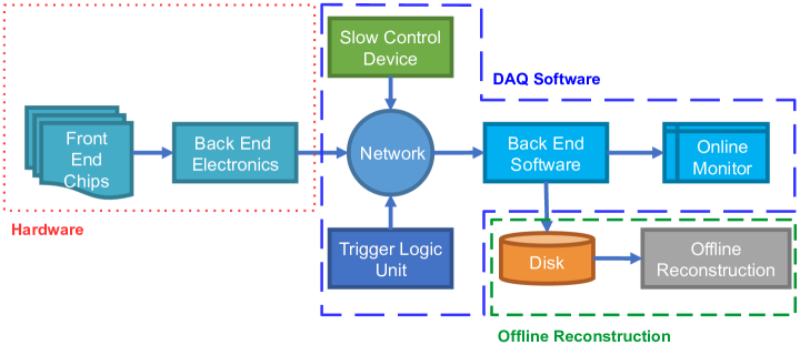
Figure 15: Flow chart highlighting the data flow in the DAQ back-end system for Lycoris.The components in the red box have been discussed in the Section 2, while the components inside the blue and green boxes are discussed in Section 3.

The back-end DAQ software runs on a Control PC, polling all the connected devices. It is responsible for collecting all the data and writing it to disk for the offline track reconstruction. Additionally, it provides online monitoring to provide a quick feedback on the data-quality during data-taking. This DAQ software for Lycoris consists of two separate layers: the layer communicating direct to the Lycoris hardware uses the Rogue DAQ framework while the interfacing of Lycoris with the AIDA TLU and the user DAQ is handled by EUDAQ2.

3.1 Rogue DAQ

The software employed to communicate with the DAQ board and KPiX chips is based on the Rogue platform [33]. Rogue was created by SLAC to facilitate development of software interfaces to hardware in DAQ systems. It has been designed with easy-to-understand mechanisms to connect independent management and data processing modules together and uses a set of well-defined and easy-to-understand interfaces. It has been developed using both C++ and Python and the interfacing between the C++ and Python parts is done using Boost.Python. Rogue provides a properly acquired and released global interpreter lock which enables true multi-threading and predefined handlers to access the data buffer pipelines and hardware interfaces, which EUDAQ2 is using to establish full control of the data taking with KPiX and Lycoris.

3.2 EUDAQ2 integration

The integration of Rogue into EUDAQ2 has been done using the Python interfaces of both packages. The Lycoris strip telescope has used two distinct versions of the KPiX DAQ system during its development history. The initial version was able to only synchronize Lycoris to an external device by merely counting the incoming triggers, while the final version can additionally synchronize the incoming triggers by timestamping with a centrally provided clock. Lycoris is using the new KPiX DAQ system which enables full synchronization with other devices such as the EUDET telescope via the AIDA TLU.

The KPiX Producer, which is a part of the EUDAQ2 package, is a Python-based Producer to operate Lycoris using the imported KPiX DAQ libraries. In the EUDAQ2 framework, the Producer acts as the interface between the user DAQ and the EUDAQ2 core components including the Run Control and the Data Collector. The EUDAQ2 Run Control is used to issue all commands to the connected Producers and the underlying DAQ systems including Lycoris. The EUDAQ2 Data Collector uses the KPiX binary data format libraries to store the incoming Lycoris data-stream and the DataConverter module converts KPiX binary format to the common format used by EUDAQ2. This is necessary to make the online monitoring in EUDAQ2 available.

Furthermore, the KPiX user module contains a customized GUI, which provides more detailed information like the data rate during a run, and an analysis executable called lycorisCliConverter, which produces a set of basic plots, e.g. the ADC distribution of each channel, and stores them into a ROOT file. Figure 16 show the interplay of the various DAQ software components.

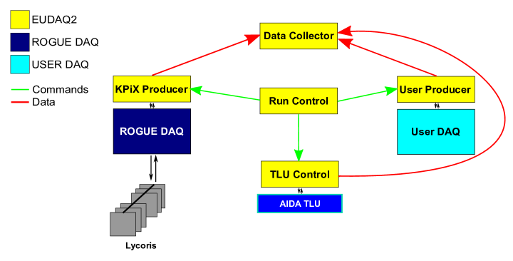
Figure 16: The interplay between the various EUDAQ2 producers and the EUDAQ2 Data Collector with the Lycoris DAQ system.

3.3 Online Monitoring & Slow Controls

3.3.1 Online Monitoring

The online monitor for data taking with the Lycoris telescope has been developed using the EUDAQ2 online monitor module StdEventMonitor. It provides a list of 2D histograms showing spatial correlations of hitted strips from two different sensor planes, which can be used to control the data quality, beam alignment and the beam spot position. Figure 17 is a screenshot of the online monitor during Lycoris data taking, where the shown example histogram shows a clear spatial correlation between the first and the third Lycoris telescope planes. Online monitor data streams are converted by the DataConverter, including data format decoding, ADC to charge conversion and baseline noise subtraction to remove pedestals and the common-mode noise, see details in Section 3.4.

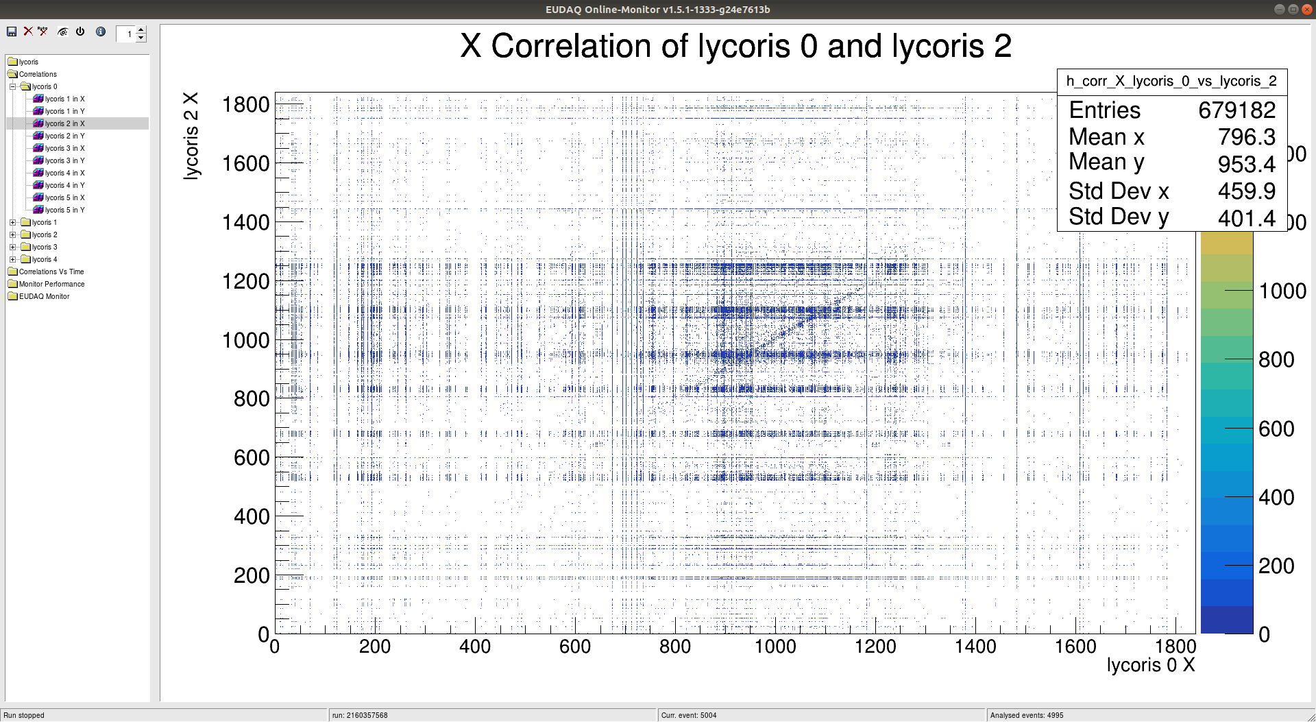
Figure 17: Online monitor showing spatial correlations of two Lycoris sensor planes from one example data taken outside the PCMAG with the EUDAQ2 and the AIDA TLU at the DESY II Test Beam Facility, where the x and y axes are in unit of the strip readout pitch ($50\text{\,}\mathrm{\SIUnitSymbolMicro m}$). This shows a good alingment between the two sensor planes and a beam spot of $20\text{\,}\mathrm{mm}$$\times$$20\text{\,}\mathrm{mm}$ (same size as the used collimator) located in the center of the sensor.

3.3.2 Slow Controls

The Lycoris slow control system monitors the humidity and temperature inside the cassette units and the bias voltages for each sensor. The humidity and temperature are monitored by an I²C sensor located on the master cassette board, which is polled by the KPiX DAQ. The HV modules of the WIENER MPOD system are controlled and monitored remotely through an SNMP v2c (Simple Network Management Protocol) compliant protocol. It is integrated into EUDAQ2 with a Producer to poll the measured current and voltage, and with one dedicated Data Collector the collected data can be stored directly in the format used by EUDAQ2.

Figure 18 shows the bias current in $\text{\,}\mathrm{nA}$ of a sensor measured over two hours during data taking, providing fast feedback on the status of each sensor.

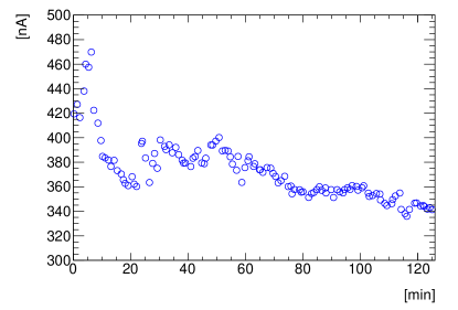
Figure 18: The bias current in nA vs. time in minute over two hours of sensor plane 0 from example data taken with the EUDAQ2 and the AIDA TLU at the DESY II Test Beam Facility.

3.4 Event Reconstruction

Two software packages are used for the track reconstruction; the first package loops over the raw data provided by Lycoris and produces hit clusters for the tracking algorithms, while the second one does the overall alignment, the track finding and fitting and produces both a fully aligned geometry and the fitted tracks. Figure 19 shows a simplified block diagram of data processing for track reconstruction with Lycoris.

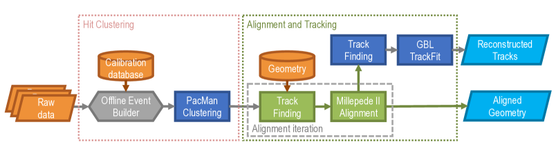
Figure 19: Flow chart of the tracking reconstruction algorithms.

3.4.1 Hit Clustering

The Hit Clustering analysis package reads in the raw data, applies the necessary corrections and then groups strips into hit clusters. The package is written in C++ and built with CMake [34]. There are two main steps in this package, the offline event builder and the PacMan clustering algorithm.

The Offline Event Builder

The first step converts the raw binary data into events suitable for reconstruction. The definition of an event depends on whether Lycoris is operated in external trigger mode or internal trigger mode (see Section 2.3.2). In external trigger mode, one event is a snapshot of the full telescope, i.e. one event consists of data from the same bucket of all 1024 channels of all KPiX chips in the same acquisition cycle. For the internal trigger mode, every readout channel is triggered individually but one event can still be defined by matching an internal trigger with an external trigger using timestamps. Therefore, one event in this case may contain data from different KPiX readout channels at different memory buckets of all the KPiX chips in the same acquisition cycle. As already explained in Section 2.3.2, Lycoris prefers to be operated using the external trigger mode and the all the following steps are targeted for this trigger mode.

The following is the baseline noise subtraction, which includes subtractions of the pedestals and the common-mode noise. The pedestal subtraction is performed separately for each memory bucket of each KPiX readout channel, and defined as the median of the charge response over a series of acquisition cycles in order to suppress the impact of outliers. The common-mode noise subtraction is applied on an event-by-event basis for each individual KPiX to ensure that data recorded in different memory buckets during different acquisition cycles are comparable. It is calculated as the median of the pedestal-subtracted charge responses of one KPiX chip for one event. Therefore, the calibration constants (see Section 2.3.2) have to be applied to convert the raw ADC value to a charge in $\mathrm{fC}$ beforehand so that charge response is comparable from one channel to another when calculating the common-mode noise.

At the end of the baseline noise subtraction, all KPiX readout channels that are not connected to a strip are removed, so every KPiX channel represents one readout strip on the sensor, and thus is referred to be the strip identity.

Before grouping strips into clusters, we apply the following quality criteria to remove strips with faulty ADC readings:

• The calibration slope has to be non-zero;

• The calibration needs to show a good linearity by requiring its Pearson correlation coefficient to be greater than $0.85$;

• The Median Absolute Deviation (MAD) of the measured charge of each bucket of each strip over all cycles must be non-zero.

The intrinsic noise level $N_{i}$ for one strip at one memory bucket is defined as the width of its noise-corrected charge response when no signal presents. For one charge measurement $q_{i}$ of one strip at one memory bucket, its significance is calculated as $q_{i}/N_{i}$. The results of the complete noise-removal procedure and the noise performance will be discussed in Section 4.

PacMan Clustering Algorithm

The next step in the chain is the clustering algorithm which follows right after the baseline noise removal. A relatively loose selection is applied on all strips before the clustering by requiring $S/N>2$ to ensure a sufficient cluster purity while retaining suitable statistics at this stage. The clustering algorithm then searches iteratively for the most significant strip as the cluster seed and groups its neighbor strips to form a cluster. For each cluster, the group process stops if the next-neighbor strip has a higher significance in order to keep clusters isolated.

The attributes assigned to each generated cluster are the charge $Q$, the significance (signal-to-noise ratio) and the cluster size (strip multiplicity). The cluster charge $Q$ is defined as the sum of the charges of all associated strips. Its noise $N$ is then calculated by adding the noise of all its associated strips in quadrature. As a result, its significance can be calculated as

$$\frac{Q}{N}=\frac{\sum^{n}_{i}q_{i}}{\sqrt{\sum^{n}_{i}N_{i}^{2}}},$$ (3.1)

where $n$ is the number of strips in the cluster, and $q_{i}$ and $N_{i}$ represent the signal charge and noise level for each associated strip. The position of each cluster perpendicular to the strip direction (the y-axis) is obtained by charge weighting

$$y_{cluster}=\frac{\sum^{n}_{i}q_{i}\cdot y_{i}}{\sum^{n}_{i}q_{i}}.$$ (3.2)

The results from the clustering procedure are called hits throughout the remainder of this section.

3.4.2 Alignment and Tracking

The alignment and tracking algorithms are part of a highly modular Python package. The three major algorithms of this package are the alignment code using Millepede II [35], the track-finding algorithm developed specifically for Lycoris and the track (re)fitting using the General Broken Lines (GBL) package [36].

For the reconstruction, the following global coordinate system is used throughout the paper: The z-axis is along the beam axis, orthogonal to the Lycoris sensor planes. The x-axis is defined to be parallel to the silicon-strips on the axial sensor and the y-axis is perpendicular to the silicon strips (See Figure 20).

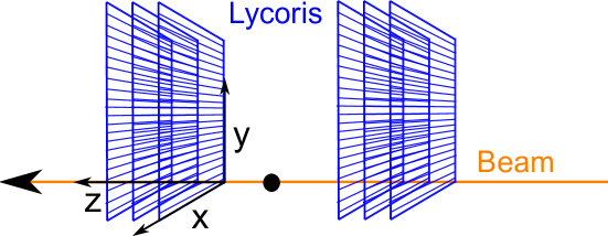
Figure 20: The global coordinate system used by the Lycoris Tracking and Alignment tool. The z-axis is along the beam axis, orthogonal to the Lycoris sensor planes. The x-axis is defined to be parallel to the silicon-strips on the axial sensor and the y-axis is perpendicular. The origin is located in the center of the telescope as indicated by the black dot.

Pre-selections

There is a series of pre-selection cuts that are applied to the raw hits before the alignment and tracking algorithm. First an event filter is applied to remove abnormal noisy events with at least 50 hits before any track finding algorithm is deployed. Subsequently, hits from the three layers in each cassette need to be correlated within a $1\text{\,}\mathrm{mm}$ window based on an initial geometry description. Hits that can not be correlated to others or hits with more than $5$ strips are all removed.

Alignment

The alignment uses the Millepede II algorithm which has already been used successfully by H1 [37, 38, 39], CMS [40, 41], BELLE-II [42] and others. Millepede II is responsible for relative position alignment, meaning a 3-D reference frame is always needed as input; which is usually given by fixing the first and the last plane of the whole tracking system. It builds on the case where least-squares fit problems with a very large number of parameters can be subdivided into two classes, global and local parameters. Millepede II then solves this to determine the alignment constants, where the global parameters are independent of the number of local parameters.

Track Finding

Two track finding algorithms are designed to reconstruct stand-alone tracks with Lycoris hits. The two algorithms can be used in any order and hits associated to one track candidate are not used for the subsequent algorithm to avoid double counting. The track model is a straight line. In the case that a magnetic field is present, a coordinate transformation is applied to tracking parameters to account for the impact of the B-field based on the beam energy.

Striplet finder:

It constructs Striplets in each cassette then matches them to form track candidates. The seed of Striplet is a doublet constructed by hits from the two stereo ($2\mathrm{°}$ stereo angle) layers in one cassette. By intersecting the two hits a 2D position is obtained in the x-y plane that is later interpolated to the axial layer for a third hit search. The third hit will be added to form the so-called Striplet when its distance to the doublet interpolation is smaller than $100\text{\,}\mathrm{\SIUnitSymbolMicro m}$. The four tracking parameters  of one Striplet are determined based on assumptions on slopes in both x-z and y-z planes for two reasons. First the three 1D measurements cannot determine four tracking parameters; second the doublet intersection needs both slopes for corrections due to the distance in z-axis between the two stereo layers. Assumptions on slopes are given by the beam direction with a correction if a magnetic field is present. Once all the Striplets are found in both cassettes, Striplet matching between cassettes starts. First their slopes on the y-z plane are matched by requiring the curvature difference to be smaller than $0.01\text{\,}\mathrm{rad}$. Then they are extrapolated to the center between two cassettes for position matching by requiring the deviation to be smaller than ($<$$10\text{\,}\mathrm{mm}$) in x and ($<$$1\text{\,}\mathrm{mm}$) in y. To increase the purity, the matched Striplets only become a valid track candidate if they are the unique match to each other.

Strip road search:

It first forms track roads using four hits from the seed layers, then adds in one to two test hits from other test layers to finalize the search. The track road needs four hits to provide the full spatial description of a track. The default choice is to use the four stereo layers as the seed layers while the two axial layers are used as test layers to maximize the x-z plane description. An event will be rejected if there are fewer than five layers with hits or any layer possesses more than eight hits. Once all track roads are found, they are interpolated to the test layers and only the unique hits within a distance of $200\text{\,}\mathrm{\SIUnitSymbolMicro m}$ are taken. The distance from the test hits to the interpolation is then used to calculate a $\chi^{2}$ to estimate the goodness of this track candidate. At the end, only the best track candidate is selected based on the number of associated hits and the goodness of fit $\chi^{2}/ndf$.

The combination of the high purity/low efficiency Striplet finder and low purity/high efficiency strip road search allows to reach a high overall track-finding efficiency to account for some possible inefficient telescope plane.

Track Fitting

After finding of all possible track candidates a re-fit of all valid track candidates using GBL is performed, taking into account all measurements and scattering materials in the path of the track. For a track with an initial trajectory from a pre-fit of the measurements (internal seed) or an external prediction (external seed) the description of multiple scattering is added by offsets in a local system. Along the initial trajectory points are defined which can describe a measurement or a (thin) scatterer (insensitive material) or both. Measurements are arbitrary functions of the local track parameters at a point (e.g. 2D: position, 4D: direction+position). The re-fit provides corrections to the local track parameters (in the local system) and the corresponding covariance matrix at any of those points. Non-diagonal covariance matrices of measurements will be diagonalized internally. Outliers can be down-weighted by use of M-estimators. A single measurement point can be omitted from the refit in order to calculate unbiased residuals.

4 Performance of the Lycoris telescope

This section presents all the results obtained using Lycoris starting from the bare sensor performance to the momentum resolution. Firstly the test-beam setups used are described, which are the basis for most results through this section.

All the shown performance studies use only data stored in the first memory bucket of each KPiX readout channel as no good-quality data have been collected using other three memory buckets. The observed symptoms for these cells are that most of the KPiX channels are found bad in either their ADC response or in their baseline noise level. The root-cause for this problem is yet to be understood, but studies conducted post data-taking, have indicated, that by increasing the $T_{\mathrm{Pre-Charge}}$ (see 2.3.2) by a factor of two, the data stored in the three other memory buckets can be recovered. Unless mentioned explicitly, all the data shown are taken in the high-gain mode using the external trigger, which is the default mode for the Lycoris telescope.

4.1 Test Beam Setup

The system performance of Lycoris telescope has been evaluated at the DESY II Test Beam Facility in several test-beam campaigns. They can be categorized into two different categories: one for performance measurements with an EUDET-style pixel telescope AZALEA outside the PCMAG solenoid; the other one for validating the system performance inside the PCMAG solenoid with the AZALEA telescope as DUT.

4.2 Operation at DESY II

The KPiX ASIC used in Lycoris requires an Acquisition Start Signal, so in order to operate Lycoris at the DESY II Test Beam Facility efficiently, several particular properties of DESY II have to be taken into account in order to synchronize Lycoris with the accelerator.

DESY II [43, 44] is a synchrotron using normal-conducting magnets with a circumference of $292.8\text{\,}\mathrm{m}$ and a maximum energy of $7.0\text{\,}\mathrm{GeV}$. Its standard operation without any extraction stores a bunch of electrons or positrons for two magnet cycles $\mathrm{T_{DESY\;Magnet\;Cycle}}$ of $80\text{\,}\mathrm{ms}$ which define the $160\text{\,}\mathrm{ms}$ DESY II cycle. One bunch of about 10¹⁰ electrons or positrons is injected on-axis at $E_{\rm min}=$0.45\text{\,}\mathrm{GeV}$$ from the linear accelerator LINAC II (LINear ACcelerator) via the accumulator storage ring PIA (Positron Intensity Accumulator) and is accelerated to $E_{\rm max}=$6.3\text{\,}\mathrm{GeV}$$. The beam is typically stored for two magnet cycles or one DESY II cycle and is then dumped about $160\text{\,}\mathrm{ms}$ after injection, just before the next injection from PIA.

The beam at the DESY II Test Beam Facility is generated using a carbon fiber, generating bremsstrahlung photons and then making electron-position pairs at a secondary target. A threshold on the particle energy $\mathrm{E}_{\rm cut}$ can be applied with a dipole magnet. Depending on the selected $\mathrm{E}_{\rm cut}$, beam will only be available if the DESY II beam energy is exceeding the selected particle energy [10], as shown in Figure 21.

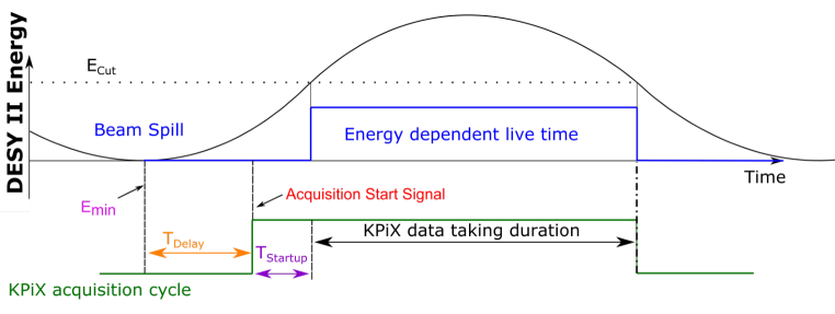
Figure 21: Synchronization of Lycoris with the DESY II accelerator cycle.

Therefore, to take data efficiently with the KPiX acquisition cycle, the Acquisition Start Signal (as described in Section 2.3.2) needs to be timed correctly that data taking commences after the DESY II beam energy exceeding $\mathrm{E}_{\rm cut}$. The $\mathrm{E}_{\rm min}$ signal from DESY II is used as a reference to generate the Acquisition Start Signal by applying a configurable delay timer $\mathrm{T_{Delay}}$, and the fixed $\mathrm{T_{Startup}}$ time of KPiX ASICs needs to be extracted in the calculation:

$$\mathrm{T_{Delay}(E_{cut})}=\frac{\mathrm{T_{DESY\;Magnet\;Cycle}}}{2\pi}\left(\arcsin\left(\frac{\mathrm{2E_{cut}-E_{max}+E_{min}}}{\mathrm{E_{max}-E_{min}}}\right)+\frac{\pi}{2}\right)-\mathrm{T_{Startup}}$$

This operation ensures that Lycoris is always ready for data taking right after particles with energy above the selected energy $\mathrm{E}_{\rm cut}$ start to arrive. The Data Acquisition period then lasts until the beam energy is below the threshold again, upon which the digitization and readout of all data take place. A sketch of the complete synchronization scheme is shown in Figure 21.

Setup outside of the PCMAG

The performance results shown in this paper are based on the latest data collected outside PCMAG in 2020 March. Lycoris was installed next to each other in between the up- and downstream arms of the AZALEA telescope, and with a close distance to the nearest AZALEA plane see Figure 22 (left). Data was taken with the beam energy threshold set at $4.4\text{\,}\mathrm{GeV}$; trigger coincidence was provided by two crossing scintillators located closely in front of the first AZALEA plane; the beam collimator is set to $x\times y=$$20\text{\,}\mathrm{mm}$$\times$$10\text{\,}\mathrm{mm}$ and the distance from the beam collimator to the first scintillator is about $220\text{\,}\mathrm{cm}$. The trigger rate under this configuration is high enough to fill all the four memory buckets of each KPiX channel at every acquisition cycle.

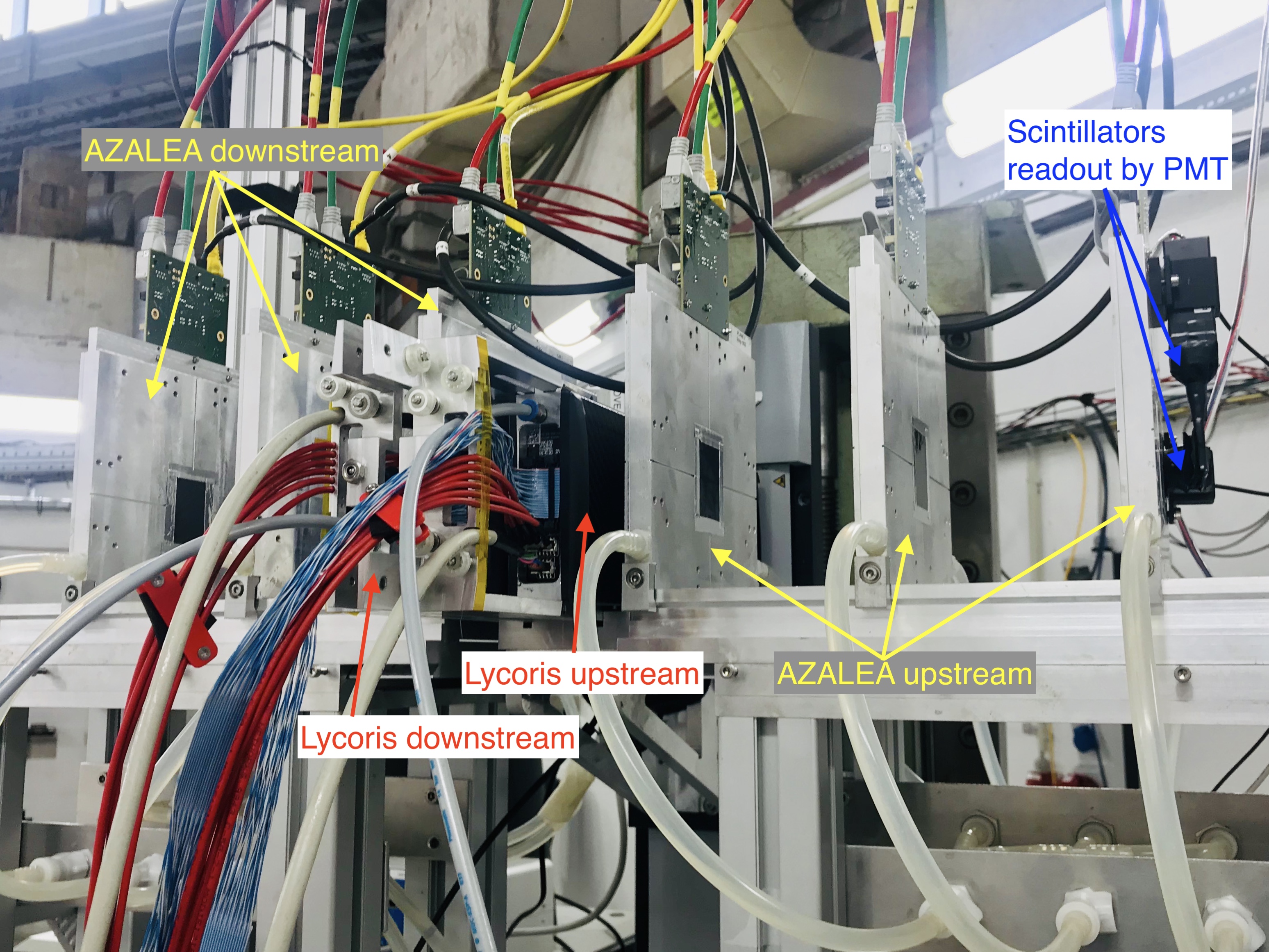
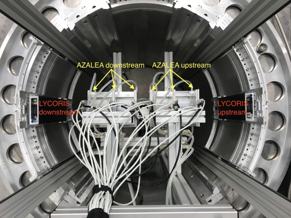
Figure 22: Setup for Lycoris tracking performance measurements with the AZALEA telescope outside the PCMAG solenoid at DESY II Test Beam Facility in March 2020 (left) and inside the PCMAG with the AZALEA telescope as a DUT in the center (right).

Setup inside the PCMAG

Lycoris was installed on its dedicated rail system with AZALEA telescope inside the PCMAG solenoid in TB24/1, see Figure 22 (right). In this configuration, AZALEA is used as a DUT for Lycoris and is installed in between the Lycoris up- and downstream cassettes. Data was taken with the magnetic field set to $0.9\text{\,}\mathrm{T}$ and a beam energy threshold at $4.4\text{\,}\mathrm{GeV}$. Three crossing scintillators are placed right after the beam collimator to provide coincidence, which is about $200\text{\,}\mathrm{cm}$ away from the solenoid wall. As TB24/1 is a subsequent area, its beam collimator is about $1157\text{\,}\mathrm{cm}$ far from the primary beam collimator. This results in a relatively low particle rate in TB24/1 with trigger coincidences varying from zero to four in one KPiX acquisition cycle.

4.3 Sensor Performance

Figure 23 shows the measured electric properties of all 29 bare sensors using a probe station. The measured IV curves (left) show that the dark current level of all sensors is very good, about 100 to $150\text{\,}\mathrm{nA}$. The backplane capacitance is measured through the bias ring with an LCR meter at $10\text{\,}\mathrm{kHz}$ AC frequency and the measured CV curve (see Figure 23 (right)) determines the depletion voltage that is at around $50\text{\,}\mathrm{V}$ for all the sensors.

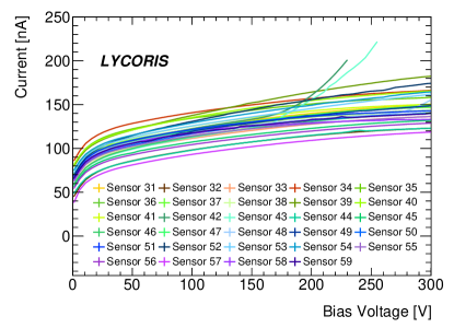
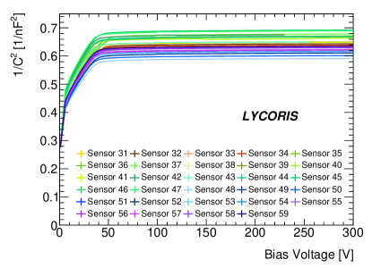
Figure 23: The IV (left) and CV (right) curves of all the bare sensors produced. 6 sensors, Sensor 59, Sensor 43, Sensor 40, Sensor 48, Sensor 47 and Sensor 46, forming an active area of 10$\times$$10\text{\,}{\mathrm{cm}}^{2}$ are used in studies in this paper.

The assembly quality is controlled by measuring the IV curve of the sensor after every major assembly step (see Section 2.3.4), namely after bump-bonding, after gluing the flex onto the sensor surface, and after wire-bonding. 22 sensors are successfully, fully assembled, and all except for two are showing an expected development. Figure 24 gives one example from the IV curves measured for the Sensor 41 during assembly. Overall, the dark current at each step stays at the same order of magnitude as the bare sensor, confirming no damage occurred to the sensor during the assembly process. The behaviors of the curves are also expected: the large increase after bump-bonding comes from impurities added from the treatment of the sensor surface during the bump-bonding procedure; the slight decrease in dark current from the "Assembled" curve (denoted for after the step of gluing the flex onto the sensor suface) to the curve after wire-bonding is understood due to an improvement of humidity of sensor storage.

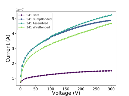
Figure 24: The IV curves of Sensor 41 at various assembly steps, where the "Assembled" refers to the assembly step after gluing the flex onto the sensor surface.

The measured bulk capacitance through bias ring of the entire sensor is $1.26\text{\,}\mathrm{nF}$ on average when fully depleted. Given the 3679 sense strips are the same in size and are coupled to the backplane in the same way, the backplane capacitance of each sense strip is therefore $1.26\text{\,}\mathrm{nF}$$/3679=$$0.34\text{\,}\mathrm{pF}$. The AC inter-strip capacitance is measured by the producer Hamamatsu when sensor is fully depleted ($60\text{\,}\mathrm{V}$) and the result on average is $8\text{\,}\mathrm{pF}$ per strip. A MIP creates about 3.5 to $4\text{\,}\mathrm{fC}$ in $320\text{\,}\mathrm{\SIUnitSymbolMicro m}$ silicon. According to the sensor design, $20\%$ of the signal charge generated in the intermediate strip goes to the backplane and the rest are shared by the neighbor strips for readout [45]. Assuming signal loss to the backplane is negligible for readout strips and the possibility to hit on a floating strip or a readout strip is equal, the expected signal charge on average is then 90% of the MIP charge thus 3.1 to $3.6\text{\,}\mathrm{fC}$.

4.4 KPiX Calibration Performance

As described in Section 2.3.2, ADC response of every readout channel is calibrated with an 8-bit DAC. The calibration data used for studies shown in this paper is taken with the most accurate configuration for the KPiX calibration system i.e. every available DAC value is measured, corresponding to 26 measurements varying from 0 to $40\text{\,}\mathrm{fC}$ for each channel. The interval of the 26 measurements is $1\text{\,}\mathrm{fC}$ from 0 to $10\text{\,}\mathrm{fC}$ and later $2\text{\,}\mathrm{fC}$ ($\sim 12500$ electrons) from 10 to $40\text{\,}\mathrm{fC}$. The slope required to convert the ADC response to $\mathrm{fC}$ (or number of electrons) can be determined by performing a linear fit on the ADC response against the DAC input value for each channel, see one example in Figure 25 (left). The kinks of single charge injection points reflect natural fluctuations at single measurement level which is not reproducible and expected. The most important is have the slope reproducible, i.e. stable charge response, which has been confirmed from various calibration data samples. Figure 25 (right) shows the distribution of the slopes of all the $1024$ channels from one KPiX.

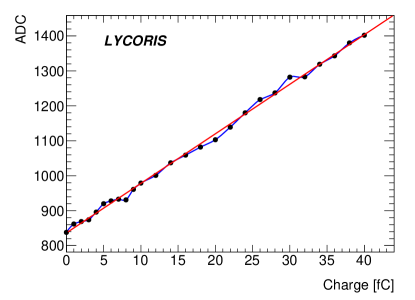
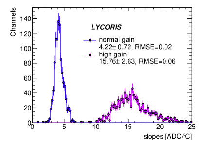
Figure 25: The ADC calibration curve of one example channel from one KPiX, a linear fit is performed in red (left). The slope distribution of the ADC response to the charge injected for all 1024 channels of a KPiX, the blue curve refers to calibration data in normal-gain mode while the violet one is using the high-gain mode; the mean value, its RMS and RMS error (RMSE) are given for each curve in the legend.

The two distributions shown were taken using the normal-gain and high-gain modes of KPiX respectively. The ratio of the mean values of the two curves is around $1:4$ as expected from the designed value of the coupling capacitors shown in Fig 7. The small RMS Error of the slope distributions in Figure 25 (right) shows a good uniformity of all channels over single KPiX chip. Figure 26 shows a profile histogram of the slope distribution in the high-gain mode for all twelve KPiX ASICs used by Lycoris, where eleven out of the twelve chips are showing a very uniform behavior.

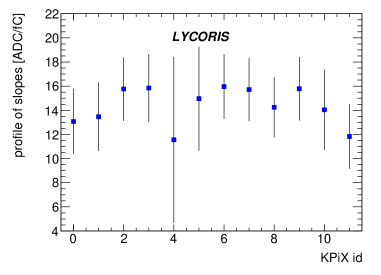
Figure 26: A profile histogram of the slope distribution of all twelve KPiX ASICs in the high-gain mode.

4.5 Module Performance

4.5.1 Noise Performance

In the external trigger mode, KPiX records the charge response of each channel when the external trigger arrives. As a result of the short opening window for one trigger and additionally due to the low particle rate at the test beam, only one to two out of the 1890 readout strips read out signal in every externally triggered event. As such, the majority of the KPiX channels are recording random noise. In this case, the charge distribution of one entire KPiX chip is expected to follow a Gaussian distribution centered at zero with outliers coming from signal contributions. The standard deviation of the Gaussian charge distribution defines the chip’s noise level and it is robustly estimated using the MAD: $\sigma=b\cdot MAD$ with $b=1.4826$ for Gaussian distributions.

As stated in Section 3.4, the baseline noise subtraction involves two steps: the pedestal subtraction and the common-mode noise subtraction. Figure 27 (left) shows the recorded charge distribution after the pedestal subtraction for one example KPiX chip, and its pedestal distribution against the KPiX channel number is shown using a candle plot in Figure 27 (right). The mean of the charge distribution is close to zero after pedestal subtraction, demonstrating the pedestal subtraction corrects the offset efficiently. However, the clearly asymmetric shape demonstrates the significant contribution from the event-by-event common-mode noise.

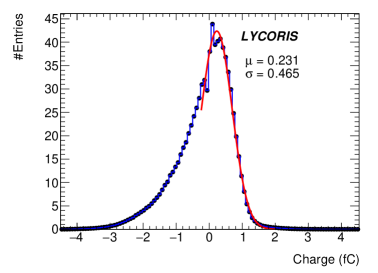
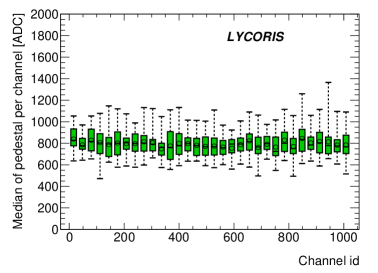
Figure 27: Charge distribution of one entire example KPiX chip after the pedestal subtraction (left) and its pedestal distribution over its channels in a candle plot (right).

After applying the common-mode subtraction, the charge distribution of the example chip shows an expected Gaussian shape with its mean value pushed closer to $0$ by two orders of magnitude, see Figure 28 (left). Besides, its width is reduced by a factor of more than two because the common-mode noise subtraction further compensate a time dependent pedestal drift which is found sufficiently uniform over time in each single KPiX chip. This pedestal drift is caused by the leakage of the charge stored in the memory buckets during the time between storage and digitization. Therefore, the amount of the drift varies according to the amount of time that the data is stored in the memory bucket before digitization, i.e. when the data was stored during the acquisition period. As a consequence, this drift is uniformly distributed over time in single KPiX chip, and thus contributing together with the common-mode noise to the asymmetric shape of the distribution in Figure 27 (left).

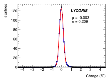
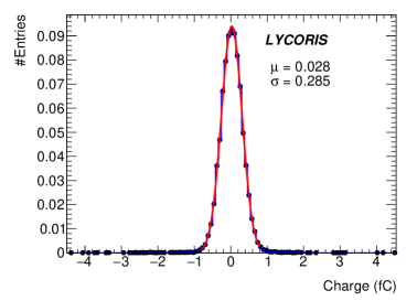
Figure 28: Charge distribution after common-mode subtraction from one entire example KPiX chip (left) and from one example KPiX channel that is connected to a strip (right).

Figure 28 (right) shows the Gaussian charge distribution read out from one example strip, i.e. one KPiX channel that connects to a strip. Its width of $0.29\text{\,}\mathrm{fC}$ defines its noise level N and with the measured charge value Q the significance can be calculated as Q/N which is the input for the subsequent clustering step.

4.5.2 Cluster reconstruction

The clusters are the reconstructed objects (see Section 3.4.1), which serve as the input hits to the alignment and tracking algorithms for track reconstruction. Figure 29 (left) shows the charge distribution of all the clusters found after clustering. A large noise peak is presents at lower cluster charges, which can be suppressed by a cut on the cluster significance. A signal amplitude of about $3.1\text{\,}\mathrm{fC}$ is expected, and the measured noise level is found to be $\sim$$0.25\text{\,}\mathrm{fC}$ on average, hence the signal-to-noise ratio ($S/N$) is expected to be $12:1$. As only every second strip is read out and 20% of the signal charge is expected to be lost to the backplane for hits on floating strips, the signal-to-noise ratio is reduced to $4.8:1$. Therefore, we applied a criterion of $S/N\geq 4$ on clusters, which serve as the input hits to the tracking algorithm. The cluster charge distribution after this selection is shown in Figure 29 (right) demonstrating a good trade-off between hit statistics and hit purity.

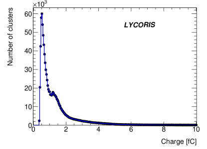
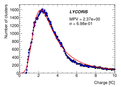
Figure 29: Charge distributions of the reconstructed clusters from one example sensor before (left) and after (right) the selection of $S/N\geq 4$.

4.6 Lycoris Performance

4.6.1 Tracking with EUDET telescope

In Lycoris performance studies, the EUDET telescope AZALEA was used to provide a reference track with which Lycoris hits can be associated to form a combined track.

Two track finding algorithms are used. They are similar to the ones used for Lycoris stand-alone track finding (see Section 3) but specialized for the pixel telescope. The two algorithms can be called in any order and all hits used to form a track candidate are not considered for the subsequent algorithm.

Triplet finder:

In each arm of AZALEA the first and the last layers are used to form doublets along the beam direction by applying a loose selection on slopes on x-z and y-z planes. To become a valid triplet, a doublet is interpolated to the middle layer to search for a matched third hit within a short distance. All valid triplets inherit the tracking parameters from the doublets and are later extrapolated to the center between the two AZALEA arms for a match. When a triplet from one arm matches to another triplet in the other arm, requiring a small deviation in both x and y as well as in the track angle in x and y, then a valid triplet track has been found. Same as for the Striplet finder, a double uniqueness is required, meaning triplets from the same doublet but different third hits will be rejected here.

Road search:

The road search first forms track roads along the beam direction using the first and the last layers of the both arms. If there are at least two other uniquely matched hits found within a short distance to the track road, i.e. at least four hits can be associated with this track, then a valid track candidate has been reconstructed.

For the combined track finding, the road search is used to associate the Lycoris hits to the track road defined by the AZALEA track candidate. One AZALEA track can be associated with up to six Lycoris hits that each is a unique match in a short distance.

4.6.2 Track Hit Performance

Track hits are the hits associated to a reconstructed track. The track hit performance shown here is using the Lycoris stand-alone tracking algorithm described in Sec 3. Figure 30 (left) shows the position of hits in local $y$ coordinate, which shows a clear 1D profile of the beam spot at the DESY II Test Beam Facility.

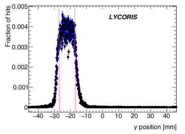
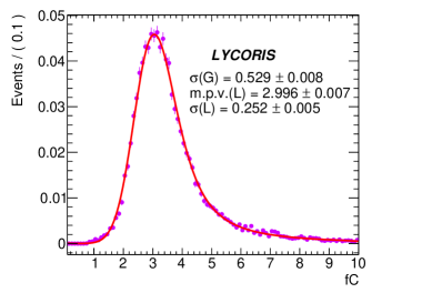
Figure 30: The hit position in the local Y-axis of all six Lycoris layers according to data taken with a beam collimator of $x\times y=$$20\text{\,}\mathrm{mm}$$\times$$10\text{\,}\mathrm{mm}$ (left), where the pink lines indicates the projection of the beam collimator size. The normalized charge distribution of all the hits on one example sensor plane associated to stand-alone Lycoris tracks, a Landau convoluted Gaussian fit is performed giving the Landau most probable value of $3.0\text{\,}\mathrm{fC}$.

Signal Amplitude

Figure 30 (right) shows the charge distribution of hits from one example sensor plane associated to stand-alone Lycoris tracks. A Landau convoluted Gaussian fit is performed giving the Landau most probable value of $2.9\text{\,}\mathrm{fC}$ and this is the measured signal amplitude for this sensor. The measured signal amplitude is consistent with the basic expectation on a MIP in this $320\text{\,}\mathrm{\SIUnitSymbolMicro m}$ thick sensor read by every other strip.

Signal-to-Noise Ratio

The signal-to-noise ratio is calculated for each hit cluster that is associated to a track, and its distribution for one of the Lycoris sensors is shown in Figure 31. The cut-off to the left is due to the quality selection of the clusters, that are used as input to the tracking algorithm while the majority of clusters are centered the mean value of $14.4$ giving a good estimate of the signal-to-noise ratio.

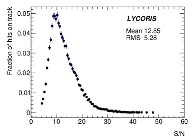
Figure 31: The signal-to-noise ratio distribution of the hits on track from one sensor.

Charge Sharing

The charge sharing has been studied with two methods in this paper. First, the spatial distribution of charge collected by the two neighbor readout strips is studied with the $\eta$ observable [46]:

$$\eta=\frac{Q_{R}}{Q_{L}+Q_{R}},$$ (4.1)

where $Q_{L}$ and $Q_{R}$ are charge collected by the two neighbor strips L and R respectively. A group of Lycoris hits with particles traversing between strips L and R are selected by demanding that its associated AZALEA track projection is between strips L and R. Figure 32 shows an example $dN/d\eta$, where contributions from different hit cluster sizes are overlaid. The $\eta$ distribution for single strip hit (cluster size 1) shows almost no charge sharing between two readout strips. This is expected as the diffusion is about a quarter of the readout pitch (half of the sense pitch). Charge sharing between readout strip and the floating strip is shown by the $\eta$ distribution for hits composed by two strips (cluster size 2). $\delta$ electron contributions is described by the curve for hits consisting of more than two strips.

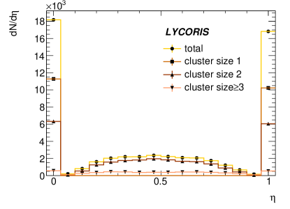
Figure 32: $dN/d\eta$ of hits from all six Lycoris layers.

Secondly, the charge sharing is studied by comparing signal amplitudes of hits from floating strips to hits from readout strips. The Lycoris hit is classified as hit generated from a readout strip if its associated AZALEA track projection is within one pitch ($25\text{\,}\mathrm{\SIUnitSymbolMicro m}$) window centered by a readout strip. Figure 33 shows the charge distributions of hits generated from floating strips (left) and from readout strips (right). The ratio of the amplitudes from the floating strip hits to the readout strip hits is about $0.85$. This means about $15\%$ charge loss to the backplane for floating strips assuming no charge loss of the readout strip hits, and this number is consistent with the designed value of $20\%$.

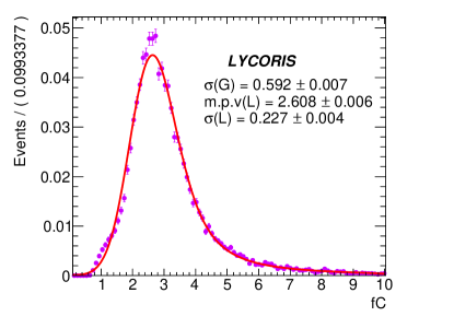
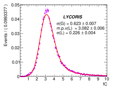
Figure 33: The charge distributions of Lycoris hits generated from floating strips (left) and from readout strips (right) and the classification on each hit uses its associated AZALEA track projection.

Cluster Size

Figure 34 (left) shows the cluster size of hits on Lycoris stand-alone tracks from one example sensor at bias voltages of $70\text{\,}\mathrm{V}$, $110\text{\,}\mathrm{V}$, and $150\text{\,}\mathrm{V}$. A slight increase on the number of single-strip clusters and a slight drop on the number of two-strip clusters can be observed with the increase of the bias voltage. It also demonstrates, that the default operation bias voltage $70\text{\,}\mathrm{V}$ is sufficient. Figure  34 (right) shows the hit cluster size for all six Lycoris sensor planes at the default bias voltage of $70\text{\,}\mathrm{V}$.

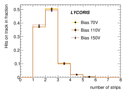
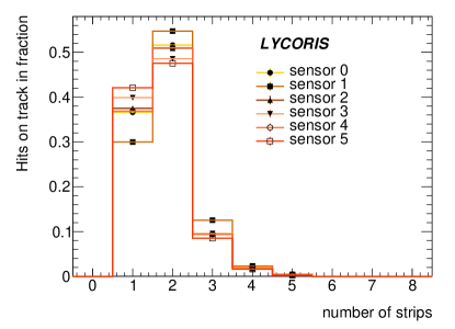
Figure 34: The hit cluster size for Lycoris standalone tracks for one example sensor at three bias voltages (left) and the hit cluster size for all Lycoris planes at the default $70\text{\,}\mathrm{V}$ bias voltage (right).

Hit Efficiency

The hit efficiency of the sensor planes has been derived using two separate approaches, using stand-alone tracks from Lycoris and using tracks from the AZALEA telescope as probe-tracks.

Assuming a similar single hit efficiency $e$ for each of the six sensor planes, the probability to get a six hits on-track is $P(6)=e^{6}$ while for five hits on-track the efficiency is $P(5)=6\cdot e^{5}(1-e)$. The ratio of six hits to five hits on-track is

$$f=\frac{P(6)}{P(6)+P(5)}=\frac{e}{6-5\cdot e},$$ (4.2)

hence the hit efficiency is $e=6f/(5f+1)$. Figure 35 shows the hit multiplicity for Lycoris stand-alone reconstructed tracks using the default hit selection used in this paper, from which the measured fraction is $0.86$ resulting in a single hit efficiency of approximately $97.3\%$.

The fake rate of the reconstructed tracks has been studied by applying the track reconstruction algorithm onto a pure noise dataset, i.e. data collected by random trigger without beam present. From a $25000$ events sample, only $29$ tracks consisting of five hits are found with a very poor $\chi^{2}$ value, validating the excellent noise rejection of the tracking algorithm developed for Lycoris.

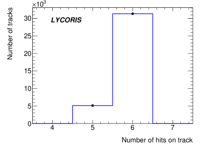
Figure 35: Hit multiplicity for Lycoris stand-alone reconstructed tracks.

An independent way to derive the single-plane tracking efficiency is to use tracks formed by AZALEA and using them as probe tracks to derive the efficiency of each Lycoris plane independently, removing any potential bias introduced by the stand-alone method. The AZALEA tracks are reconstructed using its standard reconstruction algorithms in the EUTelescope package and for the Lycoris hits to be matched, the default hit selection is used. The single-plane efficiencies found for each plane are shown in Table 4 and is very much compatible with the stand-alone method and also validating the previous assumption of very similar plane efficiencies.

4.6.3 Tracking performance

Spatial Resolution

The spatial resolution is defined as the width of a Gaussian fit of the distribution of the residuals, i.e. the spatial distance from the Lycoris measurement to the projection of the reference track provided by the AZALEA telescope. A single hit measured by Lycoris has only one axis information, the other axis information can only be obtained through the Striplet object. Therefore, the spatial resolution will be given separately.

The single point resolution for Lycoris is the resolution on the local y-axis (perpendicular to the strip direction) $\sigma_{y}$. It is given by the y-axis residuals, measured by comparing every hit on a Lycoris plane with respect to the intersection of the reference AZALEA track on this plane. AZALEA tracks can be reconstructed using Lycoris hits as input or not, respectively resulting in a biased or an unbiased measurement of the single point resolution. Figure 36 shows the biased (left) and the unbiased (right) y-axis residuals for one example Lycoris plane, each of which fits to a Gaussian well. The fitted results are both well centered at zero, showing a good alignment performance. The width of the two Gaussian fits gives a biased resolution $\sigma_{y}^{biased}=$$6.92\text{\,}\mathrm{\SIUnitSymbolMicro m}$ and an unbiased resolution $\sigma_{y}^{unbiased}=$$7.74\text{\,}\mathrm{\SIUnitSymbolMicro m}$.

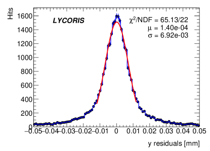
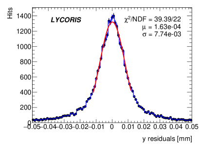
Figure 36: The biased (left) and the unbiased (right) residuals on the local y-axis (perpendicular to the strip direction) in $\mathrm{mm}$ for one example Lycoris plane.

The final single point resolution of each Lycoris sensor is estimated using the geometric mean [47] of the biased and the unbiased resolutions:

$$\sigma_{y}=\sqrt{\sigma_{y}^{unbias}\cdot\sigma_{y}^{bias}}.$$ (4.3)

Table 4 shows the unbiased, biased and the geometric mean of the single point resolution for all six sensor planes. The final single point resolution ranges from $6.92\text{\,}\mathrm{\SIUnitSymbolMicro m}$ to $7.32\text{\,}\mathrm{\SIUnitSymbolMicro m}$, significantly better than the required $10\text{\,}\mathrm{\SIUnitSymbolMicro m}$.

Sensor ID	Efficiency	$\sigma_{y}^{biased}$$\text{\,}{\mathrm{\SIUnitSymbolMicro}\mathrm{m}}$	$\sigma_{y}^{unbiased}$$\text{\,}{\mathrm{\SIUnitSymbolMicro}\mathrm{m}}$	$\sigma_{y}$$\text{\,}{\mathrm{\SIUnitSymbolMicro}\mathrm{m}}$
upstream 0	95.0%	$6.92\pm 0.06$	$7.74\pm 0.08$	$7.32\pm 0.07$
upstream 1	97.0%	$6.53\pm 0.05$	$7.33\pm 0.07$	$6.92\pm 0.06$
upstream 2	96.2%	$6.81\pm 0.06$	$7.67\pm 0.08$	$7.22\pm 0.07$
downstream 0	96.7%	$6.64\pm 0.05$	$7.41\pm 0.07$	$7.01\pm 0.08$
downstream 1	96.6%	$6.69\pm 0.05$	$7.45\pm 0.07$	$7.06\pm 0.06$
downstream 2	96.7%	$6.64\pm 0.06$	$7.59\pm 0.08$	$7.21\pm 0.07$

Table 4: The single plane hit efficiency and the three (biased, unbiased and their geometric mean) y-axis resolutions for all six sensor planes.

A single Lycoris plane measurement is not capable to retrieve information on the local x-axis (along the strip direction), while the Striplet object reconstructed from three planes in one cassette provides a 2D information with the $2\text{\,}\mathrm{\SIUnitSymbolDegree}$ stereo angle arrangement. Figure 37 shows the x-axis residuals of up- and downstream cassettes. Both residual distributions are fitted to a Gaussian that is well centered at zero. The width of the Gaussian fit gives an x-axis resolution $\sigma_{x}=$$0.224\text{\,}\mathrm{mm}$ for the upstream cassette and $\sigma_{x}=$$0.238\text{\,}\mathrm{mm}$ for the downstream cassette, exceeding the design requirement of $1\text{\,}\mathrm{mm}$ by a factor of around five.

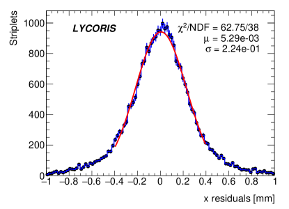
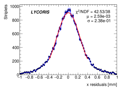
Figure 37: Residuals on the local x-axis (along the strip direction) in $\mathrm{mm}$ of Striplet from up- (left) and downstream (right) cassettes.

Momentum Resolution

The momentum resolution is defined as the error propagated on the curvature measurement of Lycoris stand-alone tracks. Data collected inside the PCMAG with the two Lycoris cassettes well separated is the ideal configuration for momentum measurements. As a result of a very low data rate inside the PCMAG and a lack of test beam time, only $251$ valid tracks have been reconstructed from the data collected by Lycoris inside the PCMAG. Therefore, a simulation is implemented to estimate the momentum resolution in this case, and the single point resolution is taken from the average measurement value of $7\text{\,}\mathrm{\SIUnitSymbolMicro m}$ shown in this paper. The simulation takes geometry input from the test beam setup of Lycoris installed inside the PCMAG, where the distance is $750\text{\,}\mathrm{mm}$ from the first to the last Lycoris planes, and the distance between sensor planes in each cassette is taken from the technical drawings. The simulated momentum resolution is $3.60\text{\times}{10}^{-3}\text{\,}{\mathrm{GeV}}^{-1}$ given the magnetic field is $1\text{\,}\mathrm{T}$. This aligns well with the desired momentum resolution of $5.0\text{\times}{10}^{-3}\text{\,}{\mathrm{GeV}}^{-1}$ expected from users for measurements inside PCMAG.

4.7 Summary

The Lycoris strip telescope has been successfully tested at the DESY II Test Beam Facility. It has demonstrated a single hit efficiency of approximately $97.3\%$. The single-point resolution orthogonal to the strip ($\sigma_{y}$) is on average $7.07\text{\,}\mathrm{\SIUnitSymbolMicro m}$ and the resolutions parallel to the strip ($\sigma_{x}$) for the up- and downstream cassettes are $0.22\text{\,}\mathrm{mm}$ and $0.24\text{\,}\mathrm{mm}$ respectively.

5 Possibilities for User DUT integration

The design of Lycoris was driven by the requirements of operating it inside the PCMAG at the DESY II Test Beam Facility, however, much care was taken to keep the design as flexible as possible. So Lycoris can also be operated at other test beam facilities world-wide, if there is a user need. Provided there is a suitable mechanical support for the cassettes, the only requirement to the facility is a suitable signal to derive a Acquisition Start Signal, in order to start up Lycoris.

The Lycoris telescope can receive an external clock and timestamp its events using this clock as a time base. Therefore, Lycoris can synchronize to a device that is able to issue or receive a common clock line and timestamp its events based on this clock. Therefore, integrating a user DUT can be realized in the following two methods:

• one is to synchronize the user DUT with Lycoris through an external trigger source, with which Lycoris is able to synchronize;

• the other is to synchronize the user DUT with Lycoris directly.

Both methods mentioned above can be used to operate Lycoris in a self or external trigger mode.

The Lycoris telescope has been designed from the beginning with a user DUT interface, that is fully compatible with the AIDA TLU and EUDAQ2, which simplifies the integration of a user DUT. By using this interface, the data taking sequencing is managed by EUDAQ2 and the synchronization is realized with the AIDA TLU. Therefore, the user DUT needs to be integrated with the AIDA TLU, which includes receiving the TLU triggers and synchronizing to the TLU events by receiving the trigger ID or timestamping the triggers using the TLU common clock.

It is also possible to integrate a DUT differently instead of using the AIDA TLU compatible interface. This can be done by synchronizing with Lycoris by providing a common clock signal through the NIM or the BNC port on the Lycoris DAQ board. Furthermore, a common external trigger can be fed through one of these ports as well. This of course requires additional engineering efforts and extra tests to verify the synchronization status and thus will vary case by case. Therefore, in this paper only basic guidelines are given for such an integration scheme:

• Lycoris needs to receive a common clock signal with a clock counter start signal $T_{0}$, and the clock has to be a fraction or multiples of $200\text{\,}\mathrm{MHz}$;

• If external triggers are going to be used, it is recommended but not necessary to veto all triggers outside the KPiX active data taking window to simplify the synchronization.

6 Summary and Outlook

The Lycoris telescope has been designed and built to meet the user requirements for a large-area coverage silicon-strip telescope for the DESY II Test Beam Facility with a resolution of better than $10\text{\,}\mathrm{\SIUnitSymbolMicro m}$.

The key building blocks are the Lycoris modules using a so-called hybrid-less design with two KPiX readout ASICs bump-bonded directly to the silicon sensor, which has a strip pitch of $25\text{\,}\mathrm{\SIUnitSymbolMicro m}$ with every second strip being read out. The entire telescope consists of six planes located in two cassettes with three modules each. The performance of Lycoris has been investigated in several test beam campaigns at the DESY II Test Beam Facility and the achieved resolution on the y-axis (orthogonal to the strip) per plane is on average $7.07\text{\,}\mathrm{\SIUnitSymbolMicro m}$. The results are consistent with the expected hit resolution of $7.2\text{\,}\mathrm{\SIUnitSymbolMicro m}$ estimated using $d/\sqrt{12}$, with $d$ corresponding to $25\text{\,}\mathrm{\SIUnitSymbolMicro m}$. This demonstrates the viability of the approach selected for Lycoris of only reading out every second strip and still maintaining the expected hit resolution. The resolutions on the x-axis (parallel to the strip) for up- and downstream cassettes are respectively $0.22\text{\,}\mathrm{mm}$ and $0.24\text{\,}\mathrm{mm}$, exceeding the $1\text{\,}\mathrm{mm}$ requirement by a factor of around five. The achieved resolutions are summarised in Table 5.

		Required	Achieved
Resolution in bending plane	$\sigma_{y}$	$<$ $10\text{\,}\mathrm{\SIUnitSymbolMicro m}$	$<$ $7.2\text{\,}\mathrm{\SIUnitSymbolMicro m}$
Resolution orthogonal to the bending plane	$\sigma_{x}$	$<$ $1\text{\,}\mathrm{mm}$	$<$ $0.24\text{\,}\mathrm{mm}$
Area coverage	$A_{xy}$	10$\times$ $10\text{\,}{\mathrm{cm}}^{2}$	10$\times$$10\text{\,}{\mathrm{cm}}^{2}$
Thickness of single station	d	$3.3\text{\,}\mathrm{cm}$	$<$ $3.5\text{\,}\mathrm{cm}$

Table 5: The key requirements for Lycoris and the achieved vlaues, where the achieved area can be extended to 10$\times$$20\text{\,}{\mathrm{cm}}^{2}$ by installing three more sensors inside each station.

Lycoris will now be rolled out to the users at the DESY II Test Beam Facility and further wishes for improvements and enhancements are to be expected. One obvious way for an improvement is possible second-generation cassette design that uses four sensor layers, two axial layers and one stereo (back-to-back) double layer in the center, which would yield three unbiased measurements on the y-axis.

References

- [1] H. Jansen et al., Performance of the EUDET-type beam telescopes, Eur. Phys. J. Tech. Instr. 3 (2016) 7.
- [2] EUDET project homepage, “EUDET: Detector R&D towards the International Linear Collider.” https://www.eudet.org/.
- [3] AIDA project homepage, “AIDA: Advanced European Infrastructures for Detectors at Accelerators.” http://aida2020.web.cern.ch/content/aida.
- [4] AIDA2020 project homepage, “AIDA2020: Advanced European Infrastructures for Detectors at Accelerators.” http://aida2020.web.cern.ch/.
- [5] J. Baudot, G. Bertolone, A. Brogna, G. Claus, C. Colledani, Y. Degerli et al., First test results of MIMOSA-26, a fast CMOS sensor with integrated zero suppression and digitized output, in Nuclear Science Symposium Conference Record (NSS/MIC), 2009 IEEE, pp. 1169–1173, Oct, 2009, DOI.
- [6] C. Hu-Guo et al., First reticule size MAPS with digital output and integrated zero suppression for the EUDET-JRA1 beam telescope, Nucl. Instrum. Methods Phys. Rev. A 623 (2010) 480.
- [7] D. Cussans, Description of the JRA1 Trigger Logic Unit (TLU), v0.2c, EUDET-MEMO 2009-04 (2009) .
- [8] P. Ahlburg, S. Arfaoui, J.-H. Arling, H. Augustin, D. Barney, M. Benoit et al., EUDAQ—a data acquisition software framework for common beam telescopes, Journal of Instrumentation 15 (2020) P01038.
- [9] T. Bisanz et al., EUTelescope: A modular reconstruction framework for beam telescope data, JINST 15 (2020) P09020 [2011.10356].
- [10] R. Diener et al., The DESY II Test Beam Facility, Nucl. Instrum. Meth. A922 (2019) 265.
- [11] M. Pivi, T. Fieguth, C. Hast, R. Iverson, J. Jaros, K. Jobe et al., ESTB: A New Beam Test Facility at SLAC, Conf. Proc. C110328 (2011) 1373.
- [12] A. Yamamoto, K. Anraku, R. Golden, T. Haga, Y. Higashi, M. Imori et al., Balloon-borne experiment with a superconducting solenoidal magnet spectrometer, Advances in Space Research 14 (1994) 2.
- [13] M. Wu, Silicon strip reference tracker at DESY, Tech. Rep. AIDA-2020-D15.2, AIDA2020, March, 2019.
- [14] P. Baesso, D. Cussans and J. Goldstein, The AIDA-2020 TLU: a flexible trigger logic unit for test beam facilities, Journal of Instrumentation 14 (2019) P09019.
- [15] Y. Liu, M. Amjad, P. Baesso, D. Cussans, J. Dreyling-Eschweiler, R. Ete et al., EUDAQ2—a flexible data acquisition software framework for common test beams, Journal of Instrumentation 14 (2019) P10033.
- [16] T. Behnke, R. Diener, U. Einhaus, U. Krämer, P. Malek, O. Schäfer et al., Recent Performance Studies of the GEM-based TPC Readout (DESY Module), in International Workshop on Future Linear Colliders, 6, 2020, 2006.08562.
- [17] F. J. Mueller, Development of a Triple GEM Readout Module for a Time Projection Chamber & Measurement Accuracies of Hadronic Higgs Branching Fractions in H at a 350 GeV ILC, Ph.D. thesis, Hamburg U., Hamburg, 2016. 10.3204/PUBDB-2016-02659.
- [18] J. Allison, K. Amako, J. Apostolakis, H. Araujo, P. A. Dubois, M. Asai et al., Geant4 developments and applications, IEEE Transactions on Nuclear Science 53 (2006) 270.
- [19] J. Allison, K. Amako, J. Apostolakis, P. Arce, M. Asai, T. Aso et al., Recent developments in Geant4, Nuclear Instruments and Methods in Physics Research Section A: Accelerators, Spectrometers, Detectors and Associated Equipment 835 (2016) 186 .
- [20] ATLAS collaboration, Technical Design Report for the ATLAS Inner Tracker Strip Detector, CERN-LHCC-2017-005 (2017) .
- [21] CMS collaboration, The Phase-2 Upgrade of the CMS Tracker, CERN-LHCC-2017-009 (2017) .
- [22] H. Aihara, P. Burrows, M. Oreglia, E. L. Berger, V. Guarino, J. Repond et al., SiD Letter of Intent, 0911.0006.
- [23] H. Abramowicz et al., The International Linear Collider Technical Design Report - Volume 4: Detectors, 1306.6329.
- [24] T. Behnke, J. E. Brau, B. Foster, J. Fuster, M. Harrison, J. M. Paterson et al., The International Linear Collider Technical Design Report - Volume 1: Executive Summary, 1306.6327.
- [25] J. Brau et al., KPiX - A 1,024 channel readout ASIC for the ILC, in 2012 IEEE Nuclear Science Symposium and Medical Imaging Conference Record (NSS/MIC), pp. 1857–1860, Oct, 2012, DOI.
- [26] “Hamamatsu Photonics Homepage.” http://www.hamamatsu.com.
- [27] “TSMC Homepage.” http://www.tsmc.com.
- [28] A. White, Development of GEM-based Digital Hadron Calorimetry using the SLAC KPiX chip, JINST 5 (2010) P01005.
- [29] J. Yu, E. Baldelomar, K. Park, S. Park, M. Sosebee, N. Tran et al., Application of Large Scale GEM for Digital Hadron Calorimetry, Phys. Procedia 37 (2012) 393 [1110.4326].
- [30] A. Steinhebel and J. Brau, Studies of the Response of the SiD Silicon-Tungsten ECal, in International Workshop on Future Linear Colliders, 3, 2017, 1703.08605.
- [31] J. Barkeloo, J. Brau, M. Breidenbach, R. Frey, D. Freytag, C. Gallagher et al., A silicon-tungsten electromagnetic calorimeter with integrated electronics for the international linear collider, Journal of Physics: Conference Series 1162 (2019) 012016.
- [32] A. Abdesselam et al., The barrel modules of the ATLAS semiconductor tracker, Nucl. Instrum. Meth. A568 (2006) 642.
- [33] ROGUE Software Developers, “ROGUE documentation.” http://slaclab.github.io/rogue/.
- [34] Kitware Inc., “CMake.” http://cmake.org.
- [35] V. Blobel, Software alignment for tracking detectors, Nucl. Instrum. Meth. A 566 (2006) 5.
- [36] C. Kleinwort, General Broken Lines as advanced track fitting method, Nucl. Instrum. Meth. A673 (2012) 107.
- [37] V. Blobel and C. Kleinwort, A New method for the high precision alignment of track detectors, in Conference on Advanced Statistical Techniques in Particle Physics, 6, 2002, hep-ex/0208021.
- [38] V. Blobel, Alignment algorithms, in 1st LHC Detection Alignment Workshop, pp. 5–12, 9, 2006.
- [39] H1 collaboration, H1 alignment experience, in 1st LHC Detection Alignment Workshop, pp. 41–50, 9, 2006.
- [40] G. Flucke, P. Schleper, G. Steinbruck and M. Stoye, CMS silicon tracker alignment strategy with the Millepede II algorithm, JINST 3 (2008) P09002.
- [41] CMS collaboration, Alignment of the CMS Silicon Tracker during Commissioning with Cosmic Rays, JINST 5 (2010) T03009 [0910.2505].
- [42] T. Bilka, K. Chilikin, D. Dossett, Y. Guan, J. Kandra, C. Kleinwort et al., Alignment and Calibration of the Belle II Detector, EPJ Web Conf. 214 (2019) 01040.
- [43] G. Hemmie, DESY II, a New Injector for the DESY Storage Rings PETRA and DORIS II, IEEE Transactions on Nuclear Science 30 (1983) 2028.
- [44] G. Hemmie, U. Berghaus, H. Bottcher, E. Dabkowski, H. R. Heller, G. Meyer et al., Design, Construction and Performance of the DESY II Magnets, IEEE Transactions on Nuclear Science 32 (1985) 3625.
- [45] T. K. Nelson. Private Communication, March, 2020.
- [46] E. Belau et al., The Charge Collection in Silicon Strip Detectors, Nucl. Instrum. Meth. 214 (1983) 253.
- [47] R. Carnegie, M. Dixit, J. Dubeau, D. Karlen, J.-P. Martin, H. Mes et al., Resolution studies of cosmic-ray tracks in a TPC with GEM readout, Nucl. Instrum. Meth. A 538 (2005) 372.