The Importance of Modeling Data Missingness
in Algorithmic Fairness: A Causal Perspective

Abstract

Training datasets for machine learning often have some form of missingness. For example, to learn a model for deciding whom to give a loan, the available training data includes individuals who were given a loan in the past, but not those who were not. This missingness, if ignored, nullifies any fairness guarantee of the training procedure when the model is deployed. Using causal graphs, we characterize the missingness mechanisms in different real-world scenarios. We show conditions under which various distributions, used in popular fairness algorithms, can or can not be recovered from the training data. Our theoretical results imply that many of these algorithms can not guarantee fairness in practice. Modeling missingness also helps to identify correct design principles for fair algorithms. For example, in multi-stage settings where decisions are made in multiple screening rounds, we use our framework to derive the minimal distributions required to design a fair algorithm. Our proposed algorithm decentralizes the decision-making process and still achieves similar performance to the optimal algorithm that requires centralization and non-recoverable distributions.

1 Introduction

Algorithmic decision making is increasingly being used in applications of societal importance such as hiring (Miller 2015), university admissions (Matthews 2019), lending (Levin 2019), predictive policing (Hvistendahl 2016), and criminal justice (Northpointe 2012). It is well known that algorithms can learn to discriminate between individuals based on their sensitive attributes such as gender and race, even if the sensitive attribute is not explicitly used (Barocas and Selbst 2016). As a result, there has been a lot of recent research on ensuring the fairness of automated (Barocas, Hardt, and Narayanan 2018), and machine-aided (Green and Chen 2019) decision making. A common way to mitigate fairness concerns is to include fairness constraints in the training process. For example, demographic parity constrains acceptance probability to be same across sensitive groups whereas equalized odds constrains acceptance probability given true outcome to be the same.

These fairness-enhanced classifiers are generally trained and evaluated on datasets containing historical outcomes and features. However, a critical (and often unavoidable) limitation of this approach is that the datasets present only one side of the reality. There are often systematic biases that determine whose data is included in (or excluded from) the datasets. For example, consider the German credit dataset (Dua and Graff 2017) that contains profiles of people whose loans were approved and the outcome measured is whether they repaid their loan or not. The phenomenon is further illustrated in Figure 1. One may train a classifier on this data that satisfies certain fairness constraints (e.g., as done by Hardt et al. (2016)) to predict potential defaulters. But when the classifier is used to decide credit-worthiness of future applicants, it can be arbitrarily unfair, even if it satisfies the fairness constraints on the training data (Kallus and Zhou 2018). The reason is, in the real-world, the classifier needs to decide for all incoming applications, whereas the training dataset only contains profiles of people who were given loans. Similar results follow for applications in recidivism prediction (Lakkaraju et al. 2017) and healthcare (Nordling 2019; Rajkomar et al. 2018).

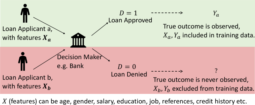
Figure 1: Missingness in Training Data due to Past Decisions

In this paper, we provide a formal framework to reason about the effect of data missingness on algorithmic fairness, a generalized version of the special cases discussed above. We use a recently proposed causal graph framework (Mohan and Pearl 2020) to model how different types of past decisions affect data missingness. We formally show, for example, that if the past decisions are fully automated, missingness in data is relatively easier to handle. On the other hand, if missingness is caused by human (or machine-aided) decisions, then it is often impossible to learn many distributions correctly, no matter how large the dataset is. This impossibility implies that the fairness guarantees of algorithms using such distributions cannot hold in practice.

Modeling data missingness also facilitates the design of better fairness algorithms for practical use. We demonstrate this by considering a multi-stage decision making scenario. At each stage of the selection process, decision makers observe new features about the individuals who pass the previous stage, and decide whether to forward an individual to the next stage or not. We show how to model data missingness in this setting using the causal graph framework and reason about the distributions that can (and can not) be used in a fair algorithm for multi-stage setting. We use these observations to propose the first detail-free and decentralized algorithm for multi-stage settings without compromising on accuracy, unlike past work that requires centralization and knowledge of non-recoverable distributions.

Summary of Our Main Contributions.

• We provide a causal graph-based framework for modeling data missingness in common scenarios from the fairness literature. We provide results on which parts of the joint data distribution can be recovered from incomplete available data and which cannot be recovered. Critically, in many scenarios of missingness, the distributions used in common fairness algorithms are not recoverable.

• We show how the above results can guide the design of fair algorithms in practice by proposing a detail-free, decentralized and fair algorithm for multi-stage setting. Our theoretical and empirical analysis on three real-world datasets shows that the algorithm provides same utility as an optimal algorithm which assumes full centralization and knowledge of non-recoverable distributions.

2 Background and Related Work

Distribution shift is a well-known problem in machine learning. This shift may be, for example, a covariate ($P(X)$) shift, a concept ($P(Y|X)$) shift or even a target ($P(Y)$) shift. While this is a broad research domain, we consider the specific setting of decision-making where the data available for training has a systematic missingness due to past decisions.

Notation.

We use the following notation throughout the paper. We use $X$ for the observed features about individuals, $U$ for the unobserved features, $Z$ for the sensitive attribute, $D$ for past binary decisions, $Y$ for the outcome realized under the given decision in the past, and $Y^{c}$ for the counterfactual outcome if the past decision was reversed. The term ‘unobserved variables’ here means that such variables are not at all measured (not considered during data collection or are impossible to be measured) whereas the term ‘missingness in data’ means that values of the observed variables are not present in some rows of the dataset.

Data Missingness in Fairness

While data missingness problem in fairness has received some attention, different papers consider different scenarios and lack a common terminology and framework for data missingness. We categorize the types of missingness studied in the fairness literature in Table 1. The first category corresponds to datasets where the outcome $Y$ is missing for certain rows and the second category addresses a bigger problem when entire rows of $(X,Y,Z)$ are missing. Thus, the first category is subsumed in the second category and addresses a relatively easier problem. Kilbertus et al. (2020) and Ensign et al. (2018) may also be placed in the first category since they consider sequential decision making settings and there is no hard constraint that $X,Z$ are missing for $D=0$. Kallus and Zhou (2018) study a setting where $X,Y,Z$ all are missing for $D=0$ and propose a weighting-based solution that assumes access to an unlabeled dataset with no missingness. We extend their work by providing a formal graphical framework to reason about missing data that can apply to any decision-making scenario.

The third category is for specialised scenarios where $D$ directly affects $Y$. The focus in our paper is on the second category where the decision itself does not affect a person’s outcome (e.g., awarding a loan does not increase the chances of a person paying it back), which is perhaps the most common setting for algorithmic decision-making. Finally, Liu et al. (2018); Hu and Chen (2018); Hu, Immorlica, and Vaughan (2019); Milli et al. (2019); Tabibian et al. (2019); Mouzannar, Ohannessian, and Srebro (2019); Creager et al. (2020) consider the effect of $D$ on future $X,Z$ distribution in sequential decision making, which is a different problem but also presents missingness related challenges.

Missingness in Variables	D affects Y?	Related Work
Only $Y$ is missing in the rows corresponding to $D=0$.	No	(Lakkaraju et al. 2017)
Entire rows ($X,Y,Z$) corresponding to $D=0$ are missing.	No	This Paper + (Kallus and Zhou 2018; Ensign et al. 2018; Kilbertus et al. 2020)
Only $Y^{c}$ is not observed, $X,Y,Z$ have no missingness.	Yes	(Jung et al. 2018; Coston et al. 2020; Kallus and Zhou 2019)

Table 1: Categorization of Related Work

Causal Graphs for Data Missingness

To model data missingness in a principled manner, we will use the causal graph framework proposed by [(Mohan and Pearl 2020; Mohan, Pearl, and Tian 2013; Mohan and Pearl 2014; Ilya, Karthika, and Judea 2015)]. The main idea in this framework is to model the missingness mechanism as a separate binary variable. If the missingness variable takes a value $0$, we observe the true value of the corresponding variable, otherwise the value is missing. Which variables affect the missingness variable decide the impact of missing data on estimating key quantities using the observed data. For example, if the missingness of a variable $X$ is caused by a variable independent from all others (e.g., a uniform random variable), then the missingness has no effect on computing $P(X)$. However, if the missingness of $X$ is caused by itself (e.g., people with $X<20$ deciding not to reveal their data), then using the d-separation criteria (Pearl 2009) and the results of Mohan and Pearl (2020), we can show that it is impossible to estimate (recover) $P(X)$. An illustrative example is included in the supplementary material; more details on identification with missing data are in Bhattacharya et al. (2020); Nabi, Bhattacharya, and Shpitser (2020).

3 Implications of Data Missingness for Fair Machine Learning Algorithms

We consider the settings where past binary decisions impact missingness in the training data $(X,Y,Z)$. If the decision $D$ for an individual was $1$, then the corresponding row containing $(X,Y,Z)$ is present in the dataset otherwise it is missing. Such missingness is perhaps the most common in datasets used in the fairness literature, including in loan decision datasets (Dua and Graff 2017) (no data from declined loan applicants) or law enforcement datasets such as search for a weapon (Goel et al. 2016) (no data for the individuals who are not searched by police). In this section, we show how missingness affects fairness algorithms by corrupting their estimation of error rates (for equalized odds (Hardt et al. 2016)), allocation rates (for demographic parity (Zafar et al. 2017)), and probabilities $P(Y|X)$, $P(Y|X,Z)$, $P(X,Z)$ and $P(X)$. All proofs are in the supplement.

Algorithms Requiring Error Rate or Allocation Rate Estimates

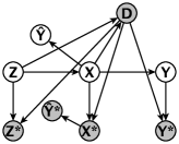
Figure 2: Data Missingness Mechanism as Causal Graph. Shaded nodes are observed, unshaded ones are not observed in the training data. For instance, the node $Y^{*}$ denotes the outcomes for people whose data is observed and $Y$ denotes the (possibly unobserved) outcomes for everyone.

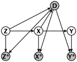
(a)

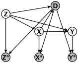
(b)

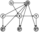
(c)

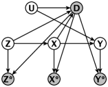
(d)

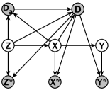
(e)

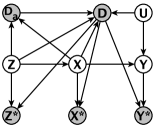
(f)

Figure 3: Data Missingness due to Fully Automated (3(a),3(b)), Human (3(c), 3(d)) and Machine-Aided Decision Making (3(e),3(f)).

Consider the causal graph shown in Figure 2. In this graph, nodes $X$, $Z$ and $Y$ represent the random variables for non-sensitive features, the sensitive attribute and the outcome respectively. For each of these nodes, we show a starred and shaded node. These nodes represent the random variables that we actually observe in the training data. Each starred node also has an incoming arrow from a “missingness variable”. In our case, this missingness variable is the same as past decisions variable $D$. $X^{*}=X$, $Z^{*}=Z$ and $Y^{*}=Y$ when $D=1$ and are missing otherwise. The incoming arrows to the missingness variable show which other variables affect the missingness in data. Figure 2 can be interpreted as showing the missingness mechanism for the lending scenario as follows: the past loan decision $D$ for an individual is based on their features $X$ (and possibly $Z$) and the features $X$ determine their payback outcome $Y$. Values for $X$, $Y$, $Z$ are observed in the training data only if $D=1$ as shown by the arrow from $D$ to $X^{*}$, $Y^{*}$, and $Z^{*}$. This causal graph captures simplistic settings but as we will show later, it is possible to represent more complex settings in a similar way. For our current discussion, this graph is sufficient.

Error Rate.

To ensure equal opportunity while predicting outcome $Y$, multiple algorithms have been proposed based on adjusting the error rates (Hardt et al. 2016; Pleiss et al. 2017) of classifiers. To obtain the error rate estimate of a classifier, the standard procedure is to use the classifier to predict $\hat{Y}$ on i.i.d. samples of the data and compare it to $Y$. However, since the data is incomplete, we do not have access to $\hat{Y}$ and $Y$. Instead, we observe $\hat{Y^{*}}$ (predictions on the available samples) and we compare them to $Y^{*}$ (outcomes for the available samples). Therefore, while the true error rate of the classifier for a group $Z$ is $P(\hat{Y}|Y,Z)$, we end up estimating $P(\hat{Y}^{*}|Y^{*},Z^{*})$ due to incomplete data. Since $P(\hat{Y}^{*}|Y^{*},Z^{*})=P(\hat{Y}|Y,Z,D=1)$ (by definition), $P(\hat{Y}^{*}|Y^{*},Z^{*})$ estimated from the available data is not equal to the true $P(\hat{Y}|Y,Z)$ unless $\hat{Y}$ and $D$ were independent given $Y$ and $Z$. Using d-separation, we can confirm in Figure 2 that $\hat{Y}\not\perp\!\!\!\perp D|Y,Z$. This leads to the following result.

Proposition 1.

For a classifier, its group error rates estimated naively from the incomplete data (with missingness mechanism shown in Figure 2) are inconsistent.

This result is neither surprising nor technically challenging to obtain but its implications are often ignored while designing fairness algorithms. The proposition implies that 1) no matter how many data samples we may have, naive error rate estimates based on data with systematic missingness will be incorrect, and 2) fairness algorithms that rely on estimating such estimates from incomplete data will fail to meet the constraints in practice. That is, if such a loan decision algorithm was deployed in practice and exposed to all applicants, fairness would not be guaranteed.

Allocation Rate.

A follow up question is whether fairness algorithms that guarantee demographic parity also fail in practice if trained on incomplete data. For demographic parity, one doesn’t need to equalize error rates across groups but only the allocation rates $P(\hat{Y}|Z)$. The question can be easily answered using a similar reasoning with the causal graph shown in Figure 2. The observed estimate of allocation rate is $P(\hat{Y^{*}}|Z^{*})=P(\hat{Y}|Z,D=1)$ whereas the true allocation rate is $P(\hat{Y}|Z)$. It is easy to see in Figure 2 that $P(\hat{Y}|Z,D=1)\neq P(\hat{Y}|Z)$ since $\hat{Y}$ is not d-separated from D given Z ($\hat{Y}\not\perp\!\!\!\perp D|Z$). We can conclude that if a fairness algorithm naively estimates allocation rates from incomplete data to enforce demographic parity constraints, then it will fail to meet the constraints on the general population.

We next show that causal graph based modeling is a powerful framework that allows us to compute general identification results by modeling data missingness in a wide variety of scenarios, including fully automated, human and machine-assisted decision-making. It is interesting to note that in our discussion, we make no assumption about the fairness or unfairness of the past decisions that cause missingness in the training data.

Algorithms Requiring Estimates of $P(Y|X)$, $P(Y|X,Z)$, $P(X),P(X,Z)$

Several algorithms in the fairness literature require distributions like $P(Y|X)$, $P(Y|X,Z)$, $P(X)$ or $P(X,Z)$ (Celis et al. 2019; Corbett-Davies et al. 2017; Valera, Singla, and Rodriguez 2018). However, it is unclear under what conditions these distributions can be recovered from the available data. We consider the different ways by which past decisions are typically made: by an algorithm, by a human, or by a human based on an algorithm’s recommendation. For each setting, we model the causal process by which the data may be missing and show how these variations effect the recoverability of true distributions from available data.

Fully Automated Decision-Making.

In fully automated decision-making, decisions are based on observed features. While a lending dataset may exclude people whose loans were not approved, for the included persons it is likely to include all features that were used by the loan approval algorithm to make its decision. Example causal graphs for this type of missingness are shown in Figures 3(a) and 3(b).

Proposition 2.

For the missingness mechanism shown in Figure 3(a), both $P(Y|X)$ and $P(Y|X,Z)$ can be consistently estimated from the incomplete data whereas $P(X)$ and $P(X,Z)$ are not recoverable.

The above proposition implies that, given enough data samples, the conditional distributions can be recovered easily from incomplete data even if past decisions were based on sensitive attributes. The main idea in the proof remains the same as we discussed for Proposition 1 i.e. using the d-separation criteria to determine whether $Y$ is conditionally independent of the missingness variable $D$ given $X$ or given $X$ and $Z$. However, the observation in this Proposition changes as soon as we relax one assumption and consider the causal graph shown in Figure 3(b) where the sensitive attribute $Z$ directly affects $Y$ (e.g., if person is likely to face direct discrimination based on $Z$ after being awarded the loan or after being hired, affecting their observed outcome).

Proposition 3.

For the missingness mechanism shown in Figure 3(b), $P(Y|X,Z)$ can be consistently estimated from the incomplete data but a naive estimate of $P(Y|X)$ is not consistent. $P(X)$ and $P(X,Z)$ are not recoverable.

The above proposition says that no matter how many data samples we have, our naive estimate of $P(Y|X)$ will not converge to the true value. However, it only establishes the inconsistency of a naive estimate of $P(Y|X)$ and it remains an interesting open question if $P(Y|X)$ is not recoverable (i.e. there exists no consistent estimator). Note that in both Propositions 2 and 3, $P(X)$ and $P(X,Z)$ are not recoverable i.e. there exist no estimators for $P(X)$ and $P(X,Z)$ that converge to the true values, even with infinitely many data samples. Non-recoverability of a distribution is a stronger result compared to non-consistency of its naive estimator. In general, if there is a direct edge between a variable and its missingness mechanism (in this case, between $X$ and $D$), then the corresponding distribution is non-recoverable (Mohan and Pearl 2020). Therefore, in typical datasets created from fully automated decision-making, it is not possible to “fix” a fairness algorithm that relies on $P(X)$ or $P(X,Z)$ by modifying the estimator. The only way is to assume external knowledge as Kallus and Zhou (2018) do or collect additional data for estimating $P(X)$. In further discussion, we will only focus on $P(Y|X,Z)$, $P(X)$ and $P(X,Z)$ and will assume $Z$ does not directly affect $Y$.

	(Pleiss et al. 2017) with FPR Constraints	(Pleiss et al. 2017) with FNR Constraints	(Kamiran et al. 2012) with SP Constraints	(Kamiran and Calders 2012)	(Celis et al. 2019) with FDR Constraints ($\tau_{fdr}=0.8$)
ADULT	FPRD: $0.0725$ ($-0.00724$)	FNRD: $0.0377$ ($0.00295$)	SPD: $-0.1137$ ($-0.0390$)	SPD: $-0.2410$ ($-0.0705$) DI: $0.5566$ ($0.7785$) AOD: $-0.1486$ ($0.0188$) EOD: $-0.1327$ ($0.0293$)	$\gamma_{fdr}$ $0.68$ ($0.63$)
COMPAS	FPRD: $0.061$ ($-0.00155$)	FNRD: $0.099$ ($0.0056$)	SPD: $-0.2651$ ($0.0229$)	SPD: $-0.2340$ ($-0.1188$ ) DI: $0.7402$ ($0.8342$) AOD: $-0.2237$ ($-0.0946$) EOD: $-0.2266$ ($0.0111$ )	N/A

Table 2: Difference in Test (and Train) Performance of Fair ML Algorithms under Training Data with Missingness. FPR stands for false positive rate, FNR for false negative rate, FDR for false discovery rate, SP for statistical parity, AO for average odds, EO for equal opportunity, DI for disparate impact, and $\gamma_{fdr}$ is the meta-fair classifier’s fairness metric (closer to $1$ is better for DI and $\gamma_{fdr}$). The suffix D denotes the difference in corresponding metric between the privileged and the unprivileged groups.

Human Decision-Making.

A distinguishing characteristic of human decision-making is that it may involve unobserved features. Lakkaraju et al. (2017) provide an example: a human judge can observe whether a defendant is accompanied by their family during trial and this may also affect their outcome (whether they recidivate or not). In the resulting training data, however, this feature may be absent (therefore, called unobserved). In addition, the recidivism outcome and features would only be available for defendants that were released. To illustrate, consider the causal graphs shown in Figures 3(c) and 3(d) (obtained from Figure 3(a) by adding $U$ for unobserved features). The difference between Figures 3(c) and 3(d) is whether $U$ affects $Y$ directly or through $X$.

Proposition 4.

For the missingness mechanism shown in Figure 3(c), $P(Y|X,Z)$ can be consistently estimated whereas for the mechanism shown in Figure 3(d), $P(Y|X,Z)$ is not recoverable. $P(X)$ and $P(X,Z)$ are not recoverable in either of the two mechanisms.

Machine Aided Decision-Making.

Another common form of decision making is machine aided decision making or algorithm-in-the-loop decision making. In this case, a human receives feedback from an algorithm before making their decision. Consider the causal graphs shown in Figures 3(e) and 3(f) (obtained from previous graphs by adding a variable $D_{a}$ representing algorithm’s feedback).

Proposition 5.

For the missingness mechanism shown in Figure 3(e), $P(Y|X,Z)$ can be consistently estimated from the incomplete data whereas for the mechanism shown in Figure 3(f), $P(Y|X,Z)$ is non-recoverable. $P(X)$ and $P(X,Z)$ are not recoverable in both these cases.

The above proposition implies that the new variable $D_{a}$ in hybrid decision making doesn’t pose additional challenges in the estimation of $P(Y|X,Z)$ distributions but the usual challenges due to human involvement continue to exist.

Empirical Implications of Data Missingness

Kallus and Zhou (2018) showed that a supposedly equal opportunity classifier of Hardt et al. (2016) trained on New York Stop, Question and Frisk dataset (NYCLU 2017) does not ensure equal opportunity in the general NYC population: it wrongly targets up to 20% of white-Hispanic, 16% of other, and 14-15% of black innocents, but only 11% of white-non-Hispanic innocents. We present several semi-synthetic experiments using the Adult (Dua and Graff 2017) and the COMPAS (Larson et al. 2016) datasets to show that this is a more general phenomenon, across different datasets, algorithms and fairness metrics.

We created synthetic missingness in these datasets based on the following procedure. We trained a logistic regression classifier from the scikit-learn library (Pedregosa et al. 2011) and then deleted the records from the training set for which the classifier’s predicted probability for the favourable class was below a certain threshold. We chose the threshold to be low enough ($0.06$ for Adult and $0.55$ for COMPAS) to ensure that the label distribution in the resulting dataset does not become very skewed. We did not delete any record from the test set (preserving the general distribution without any missingness). Note that such semi-synthetic experiments are necessary because of the unavailability of datasets with and without missingess. We then trained fairness algorithms with different underlying principles (pre-processing, in-processing and post-processing) on this semi-synthetic training data, using example code provided in IBM’s AI Fairness 360 library (Bellamy et al. 2019). In particular, we studied the calibrated equalized odds post-processing algorithm of Pleiss et al. (2017), the reject option classifier of  Kamiran, Karim, and Zhang (2012), the re-weighting pre-processing algorithm of  Kamiran and Calders (2012), and the meta-fair classifier of Celis et al. (2019). The choice of fairness metrics and datasets in the experiments is governed by the example code provided for respective algorithms. For the meta-fair classifier, we set the $\tau_{fdr}$ hyper-parameter to $0.8$ as provided in the example code.

The results are summarized in Table 2. For every algorithm, we compare the fairness measures observed on the test set and the censored training set (in parenthesis). For the pre-processing algorithm by Kamiran and Calders (2012), we show the fairness measures on the test set when there is synthetic missingness in the training set, and in parenthesis, we show the fairness measures on the test set when there is no missingness in the training set. The table shows that all algorithms show significant disparities in their fairness metric due to missing data. In many cases, there is an order of magnitude difference (over 10X) between the fairness metric on the test and (censored) train data, validating our theoretical claims about the implications of data missingness.

Discussion

Importance of Knowing Precise Causal Structure.

While the causal graphs we discussed are not exhaustive, the framework (and the same proof technique) can be used for deriving recoverability results in any new scenario. We also note that it is not enough to only model the existence of relation between variables; the direction of the causal relation is also important. For example, throughout our discussion, we assumed that the features $X$ cause the outcome $Y$. However, in some settings, the reverse may be true. That is, the target variable $Y$ (e.g. skill $Y$) of a person causes/determines their features $X$ (e.g. test scores). This may affect the conclusions about estimation of distributions. Consider, for example, the graph shown in Figure 3(c). Reversing the edge between $X$ and $Y$ in this graph affects the corresponding observation stated in Proposition 4: a naive estimate of the distribution $P(Y|X,Z)$ is not consistent in the new graph. Thus, it is important to understand the domain of interest and reason about the effects of the data censoring mechanism on the learning algorithms accordingly.

Better Data Collection Practices.

While missingness in the labels is unavoidable, missingness in the unlabeled data can be avoided by adopting better data collection practices. This may be exploited to provide better fairness guarantees, as in  Kallus and Zhou (2018). Similarly, challenges due to human involvement can be addressed by designing data (features) collection process that better capture human decision-making, or by exploiting random variations that remove the effect of unobserved variables (Kleinberg et al. 2017).

4 Application: Multi-Stage Decision Making

The framework and the results presented in the previous section are not only useful for critically evaluating existing fairness algorithms but also for designing new algorithms. In this section, we present one such example: the case of multi-stage decision-making. Multi-stage processes are common, e.g., in hiring, university admissions and even in lending. At each stage of the selection process, decision makers request or collect new features about the individuals and make decisions on whether to forward an individual to the next stage or not. Each stage of the selection process narrows down (subject to budget constraints) the pool of individuals and more features are observed in the subsequent stages for individuals who pass the previous stage.

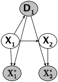
(a) Stage 1

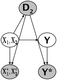
(b) Stage 2

Figure 4: Data Missingness in 2-Stage Process ($Z\in X_{1}$)

Figure 4 shows an example of a 2-stage decision process for hiring where stages represent independent organizations or teams evaluating the applicants (e.g., a recruitment agency in the first stage and the hiring entity itself in the second stage). As before, the decision $D_{1}$ in the first stage causes missingness in the features $X_{1}$ and the first stage’s outcome (whether additional features $X_{2}$ are collected for the individual). Similarly, in the second stage, the decision $D_{2}$ selects the final individuals and affects missingness of both $(X_{1},X_{2})$ and the outcome $Y$: success outcome $Y$ is observed only for individuals who passed the second stage (and consequently, also the first stage). Typically, $(X_{1},X_{2})$ is also recorded only for those individuals.

Proposition 6.

For the 2-stage missingness mechanism shown in Figure 4, $P(Y|X_{1})$ and $P(Y|X_{1},X_{2})$ can be recovered from the incomplete data but joint distribution $P(X_{1},X_{2})$ is not recoverable.

Consider a scenario where an incomplete dataset (resulting from past multi-stage decision making as shown in Figure 4) is available for learning distributions that we can use for a future application (which again is a similar multi-stage decision making application). Emelianov et al. (2019) propose an algorithm for a multi-stage decision-making application. However, the algorithm assumes full knowledge about the joint distribution of all features of the population, which according to Proposition 6 is not recoverable from incomplete data. Moreover, in decentralized settings each stage makes decisions on its own and feature distribution of all the applicants may not be shared between stages. Therefore, we explore another dimension of the solution space, which is to design algorithms without requiring distributions that cannot be recovered from incomplete data.

The $\bm{DF^{2}}$ Algorithm for Detail-Free, Decentralized and Fair Multi-Stage Decision Making

Problem Formulation.

Given a pool/batch of individuals, we want to find optimal decision rules $D_{i}$ for each stage $i$ such that the precision of the decision rule is maximized subject to constraints on the budget (fraction of individuals to be selected at that stage) and fairness. We assume that additional features are observed at each stage, so stage 1 observes $X_{1}$ features, and stage $i$ observes $\{X_{1},X_{2},...X_{i}\}$ features. Emelianov et al. (2019) have shown that when the budget is fixed, maximizing precision is equivalent to maximizing true positive rate, true negative rate, accuracy and f1-score; and minimizing false positive rate and false negative rate. Let $Y$ represent the true outcome (i.e. success in job) and $\hat{Y_{i}}$ denote the action taken for an individual at stage $i$ (whether the individual is given a job or not). $D_{i}$ is the optimization variable at stage $i$. It is a vector of real numbers between $0$ and $1$. The size of $D_{i}$ is equal to the total number of individuals at stage $i$. For an individual $j$, $D_{i}[j]$ is the probability of being selected at $j$th stage, i.e., probability that $\hat{Y_{i}}=1$. Assume $k$ stages in the entire process.

$\bm{DF^{2}}$ Algorithm.

The $DF^{2}$ algorithm solves the following optimization problem at every stage $i\in\{1,2,\dots k\}$:

$$\max_{D_{i}} P(Y=1|\hat{Y_{i}}=1)$$ (1)

s.t. $$P(\hat{Y_{i}}=1)=\alpha_{i}$$

$$f_{i}(\hat{Y_{i}})=0$$

where $P(Y=1|\hat{Y_{i}}=1)$ is the precision of the decisions taken at stage $i$, $P(\hat{Y_{i}}=1)=\alpha_{i}$ is the budget constraint at stage $i$, and $f_{i}(\hat{Y_{i}})=0$ is the fairness constraint at stage $i$.

Precision $P(Y=1|\hat{Y_{i}}=1)$ can be replaced by an empirical estimate using the conditional risk scores $P(Y|X_{1},\dots,X_{i})$ of the individuals at stage $i$, where {$X_{1},\dots,X_{i}\}$ is the set of features observed by the algorithm at stage $i$. We assume that the sensitive attribute is observed in the first stage, i.e. $Z\in X_{1}$. Let $n_{i}$ be the total number of individuals at stage $i$,

$$P(Y=1|\hat{Y_{i}}=1)\approx\frac{1}{\alpha_{i}}\sum_{j=1}^{n_{i}}\frac{D_{i}[j]\cdot P_{j}(Y|X_{1},\dots,X_{i})}{n_{i}}$$

For budget constraint on the fraction of individuals selected at stage $i$, we define this fraction w.r.t to the total number of individuals in the first stage (i.e. $n_{1}$). The constraint can be written as follows using an empirical estimate:

$$P(\hat{Y_{i}}=1)\approx\frac{\sum_{j=1}^{n_{i}}D_{i}[j]}{n_{1}}$$

Demographic parity fairness constraint is $P(\hat{Y_{i}}=1|Z=b)-P(\hat{Y_{i}}=1|Z=w)=0$; $Z$ being the sensitive attribute. Equality of opportunity fairness constraint is $P(\hat{Y_{i}}=1|Y=1,Z=b)-P(\hat{Y_{i}}=1|Y=1,Z=w)=0$. The probabilities in fairness constraints can again be replaced by their empirical estimates and in terms of only the decision variables $D_{i}$, the sensitive attribute $Z$ and the conditional distribution $P(Y|X_{1},\dots,X_{i})$. We thus get a linear optimization problem in the decision variables $D_{i}$. Note that we only used the conditional distributions $P(Y|X_{1}\dots X_{i})$ in the optimization problem, and as discussed earlier, these distributions can be consistently estimated from incomplete data. We enumerate the steps of $DF^{2}$ in a two stage process for more clarity in the supplementary material.

Advantages of $\bm{DF^{2}}$.

While the primary advantage of $DF^{2}$ is that it doesn’t require knowledge about the joint distributions $P(X_{1},\dots,X_{k})$ (hence the name detail-free), it also offers another interesting advantage over the optimal algorithm of Emelianov et al. (2019). Theirs is essentially a centralized approach assuming that a single decision maker is controlling all stages of the selection process and thus, is able to find and enforce the optimal parameters for each stage. But in many realistic scenarios, independent agencies are responsible for implementing different stages without any communication or data sharing. The $DF^{2}$ algorithm is a decentralized approach and each stage can make its decisions independently of others, without communication.

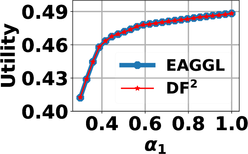
(a) ADULT

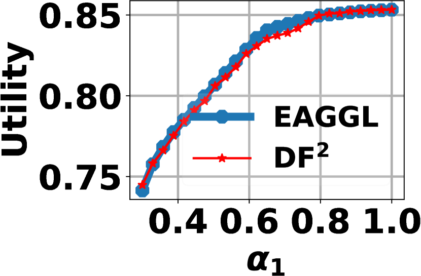
(b) GERMAN

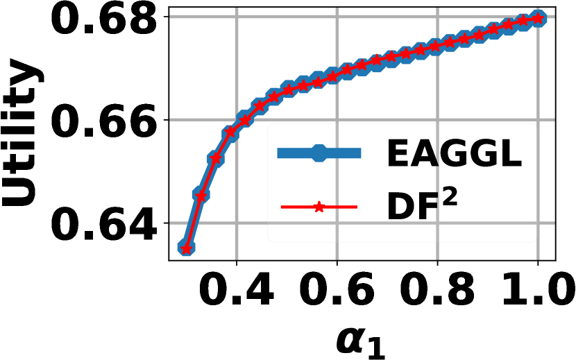
(c) COMPAS

Figure 5: Demographic Parity Fairness Constraints

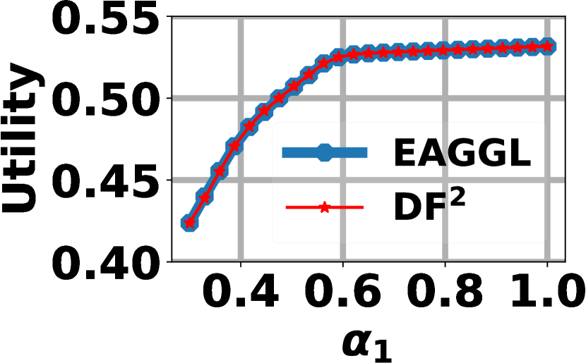
(d) ADULT

(e) GERMAN

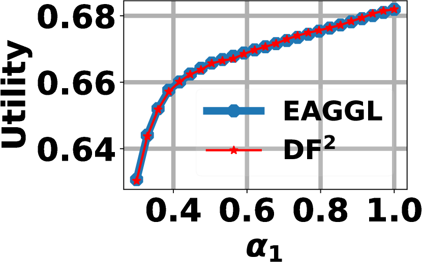
(f) COMPAS

Figure 6: Equality of Opportunity Fairness Constraints

Theoretical Analysis

While our proposed algorithm offers the advantages of being detail-free and decentralized, an important question is whether it returns a solution with lower precision compared to an optimal algorithm (an oracle algorithm that knows the joint distribution)? Consider a two stage selection process with fairness constraints and $\alpha_{1}$ and $\alpha_{2}$ budget constraints in the two stages. Let $r_{1}$ and $r_{2}$ denote the random variables $P(Y|X_{1})$ and $P(Y|X_{1},X_{2})$. We know from (Menon and Williamson 2018; Corbett-Davies et al. 2017) that optimization problem of the form used in $DF^{2}$ results in subgroup specific thresholds on the risk scores (i.e. individuals above their subgroup specific threshold are selected and everyone else is rejected). Let $\delta_{z}(\alpha_{1})$ be the threshold (for a subgroup $z$) on $r_{1}$, and let $\delta_{z}(\alpha_{2})$ be the threshold on $r_{2}$ assuming that the first stage doesn’t exist (i.e. all individuals from the first stage are made available to the second stage). Let $\alpha_{2}<\alpha_{1}<1$, which implies that $\delta_{z}(\alpha_{2})>\delta_{z}(\alpha_{1})$ since lower budget means higher threshold. Further, let $D$ denote $DF^{2}$’s output decision vector for all individuals that were initially present in the first stage (i.e. $D[j]=1$ for individuals selected in the final stage by the $DF^{2}$ algorithm and $D[j]=0$ for everyone else). Let $D^{O}$ be the output decision vector of an oracle algorithm for same pool of individuals, budget and fairness constraints. We further assume:

Assumption 1 (Coherent Features Assumption).

For any $m^{\prime},m\in[0,1]$ such that $m^{\prime}\geq m$, the following is true

$$P(r_{1}\geq\delta_{z}(\alpha_{1})|r_{2}\geq m^{\prime})\geq P(r_{1}\geq\delta_{z}(\alpha_{1})|r_{2}\geq m)$$

This fairly weak assumption intuitively means that knowing that someone has a higher $r_{2}$ does not decrease the probability of their $r_{1}$ being above a threshold. The assumption is quite natural if the feature sets $X_{1}$ and $X_{1},X_{2}$, in expectation, provide coherent information about the outcome $Y$. For example, when filtering job candidates, extra information (such as letters of recommendation) may be collected at a second stage. The assumption states that, on average, LoRs and first-stage scores don’t provide conflicting information.

Theorem 1.

Under the coherent features assumption, for budget constraints given by $\alpha_{1}$ and $\alpha_{2}$ on the fraction of individuals selected in the first and second stages, respectively, and demographic parity or equal opportunity constraint w.r.t outcome $Y$, the probability that $DF^{2}$’s output decision vector $D$ has lower precision compared to the oracle’s output decision vector $D^{O}$ (i.e. $P(D\neq D^{O})$) is upper bounded as

$$P(D^{O}\neq D)\leq P(r_{1}<\delta_{z}(\alpha_{1})|r_{2}=\delta_{z}(\alpha_{2})),$$

where $r_{1}$ and $r_{2}$ denote the random variables $P(Y|X_{1})$ and $P(Y|X_{1},X_{2})$, $\delta_{z}(\cdot)$ denotes the subgroup specific threshold discussed above, and $P(\cdot)$ denotes probability.

The above theorem shows that the probability of getting a suboptimal solution in $DF^{2}$ depends on: 1) the distribution of the risk scores $r_{1}$ and $r_{2}$ (which are derived from the feature sets $X_{1}$ and $X_{1},X_{2}$ respectively) used in the two stages, and 2) the budgets $\alpha_{1}$ and $\alpha_{2}$ of the two stages. With increasing positive correlation between $r_{1}$ and $r_{2}$ (e.g., more agreement between first-stage scores and LoR), and an increasing gap between the budgets $\alpha_{1}$ and $\alpha_{2}$ (e.g. final hiring being very selective compared to first stage screening), the probability of getting a suboptimal solution decreases. The analysis can be similarly extended to a $k$-stage process. In the next section, we empirically show that on real datasets, our algorithm’s performance is similar to the oracle algorithm.

Empirical Analysis

Datasets.

We use three real datasets for evaluation that were also used by Emelianov et al. (2019). In the ADULT dataset (Dua and Graff 2017), the outcome variable is salary and the sensitive attribute is gender. In the COMPAS dataset (Larson et al. 2016), the outcome variable is recidivism within two years and sensitive attribute is race. In the GERMAN dataset (Dua and Graff 2017), the outcome variable is returns which represents if an applicant paid back a loan and sensitive attribute is gender. We discretize all the features using the same procedure as Emelianov et al. (2019) (using their open source code on github). Details about the datasets and data processing are in the supplement.

Methodology

We simulated a two stage process using the same sequence of feature observations in the two stages as  Emelianov et al. (2019). In the ADULT dataset, the first stage observes gender, age, education while the second stage includes the previous features plus relationship and native country. In the COMPAS dataset, the first stage observes race, young (younger than 25) and drugs (arrest due to selling or possessing of drugs) while the second stage includes the previous features plus old (older than 45), gender, long sentence (sentence was longer than 30 days). In the GERMAN datatset, the first stage observes gender, job (is employed), housing (owns house), while the second stage includes the previous features plus savings (more than 500 DM), credit history (all credits payed back duly) and age (older than 50). We refer the method by Emelianov et al. (2019) as EAGGL and consider it the oracle method since it uses a centralized algorithm assuming knowledge of the full joint distribution. We compare the utility (equivalent to precision as discussed earlier) achieved by the $DF^{2}$ and the EAGGL (oracle) algorithms under fairness constraints (both methods return solutions satisfying fairness constraints). The purpose of our empirical analysis is to establish that it is possible to design fair algorithms without using non-recoverable distributions, with similar performance. The algorithm was implemented was in Python using CVXPY.

Observations.

Figures 5(a), 5(b) and 5(c) show the comparison between utility achieved by DF² and that by EAGGL in the three datasets, with demographic parity fairness constraints. The budget of the second stage was fixed at 0.3 ($\alpha_{2}=0.3$) to match the simulation parameters used by Emelianov et al. (2019). The budget of the first stage $\alpha_{1}$ was varied from $0.3$ to $1$. Clearly, the utility of DF² matches the optimal utility as achieved by EAGGL. Figures 5(d), 5(e) and 5(f) show the same trend for equality of opportunity fairness constraints as well. We note that EAGGL uses inequality in the budget constraints in non-final stages unlike $DF^{2}$ which uses equality in the budget constraints in all the stages. However, in our experimental data, we found that despite the inequality constraints, EAGGL uses the entire budget available to maximize the precision. So, this difference in optimization constraints is not a factor to be concerned about while drawing conclusions from the results. We observed similar results in a three stage process as well (details in the supplement).

Global Fairness.

Fairness constraints we discussed so far are also referred to as “local” in multi-stage settings (Emelianov et al. 2019). Unlike local fairness (that requires fairness at every stage), the concept of global fairness requires only the final stage to enforce fairness. Local fairness is a stronger concept (and in theory, a more costly one) compared to global fairness. As shown in (Emelianov et al. 2019; Bower et al. 2017), local fairness implies global fairness but the opposite is not true. Local fairness may be a more desired property in decentralized settings where individual stages are accountable for their own decisions and there is no central authority accountable on the behalf of all of them. $DF^{2}$, by design, satisfies both local and global fairness. Figure 7 shows that the difference in utilities of $DF^{2}$ with local (and thus also global) fairness constraints and EAGGL with only global fairness constraints is marginal.

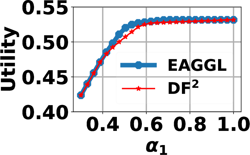
(a) ADULT

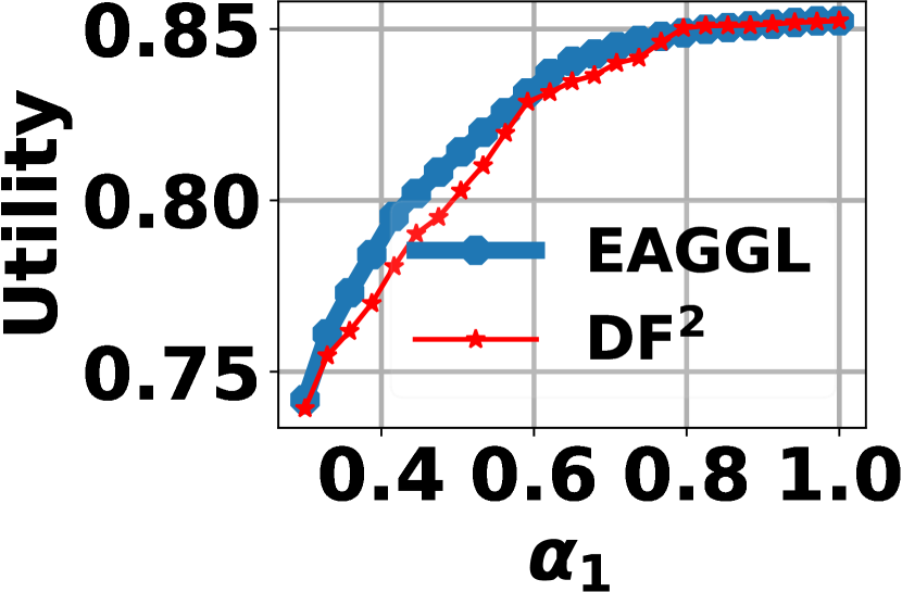
(b) GERMAN

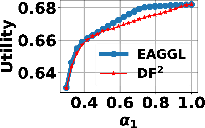
(c) COMPAS

Figure 7: EAGGL(Only Global Fairness) vs $DF^{2}$

5 Conclusions

Our results show that data missingness has significant implications for fairness algorithms and that it is important to model the missingness mechanism to accurately train fair classifiers. We used causal graphs to model missingness mechanisms in data for various real-world scenarios and discussed implications of missingness on correctly estimating distributions used in common fairness algorithms. Our results also provide useful perspective on correct data collection practices for fairness in machine learning. While the graph structures we discussed are not exhaustive, our framework can be applied to new settings by utilizing the causal structure to determine recoverability of quantities of interest. As an example, we applied our framework to develop a fair multi-stage decision making algorithm that requires no centralization between stages and uses only distributions that are recoverable from incomplete data.

Ethical/Societal Impact Statement

This paper discusses a fundamental assumption of availability of uncensored training data behind many fairness algorithms, that mostly does not hold in practice. We hope that the paper will be helpful in designing fair algorithms in the absence of this assumption. While disposing of this assumption may be possible in many settings, there may be new assumptions that may have to be introduced in the process. Specifically, we assumed knowledge of the causal graph and in the case of multi-stage decision making, the coherent feature assumption. It is always important to evaluate the suitability of such assumptions in specific applications since the performance and fairness of the algorithm may be unpredictable if the assumptions are not suitable for the given application.

References

- Barocas, Hardt, and Narayanan (2018) Barocas, S.; Hardt, M.; and Narayanan, A. 2018. Fairness and machine learning: Limitations and Opportunities.
- Barocas and Selbst (2016) Barocas, S.; and Selbst, A. D. 2016. Big data’s disparate impact. California Law Review 104: 671.
- Bellamy et al. (2019) Bellamy, R. K.; Dey, K.; Hind, M.; Hoffman, S. C.; Houde, S.; Kannan, K.; Lohia, P.; Martino, J.; Mehta, S.; Mojsilović, A.; et al. 2019. AI Fairness 360: An extensible toolkit for detecting and mitigating algorithmic bias. IBM Journal of Research and Development 63(4/5): 4–1.
- Bhattacharya et al. (2020) Bhattacharya, R.; Nabi, R.; Shpitser, I.; and Robins, J. M. 2020. Identification in missing data models represented by directed acyclic graphs. In Uncertainty in Artificial Intelligence, 1149–1158. PMLR.
- Bower et al. (2017) Bower, A.; Kitchen, S. N.; Niss, L.; Strauss, M. J.; Vargas, A.; and Venkatasubramanian, S. 2017. Fair pipelines. arXiv preprint arXiv:1707.00391 .
- Celis et al. (2019) Celis, L. E.; Huang, L.; Keswani, V.; and Vishnoi, N. K. 2019. Classification with fairness constraints: A meta-algorithm with provable guarantees. In Proceedings of the Conference on Fairness, Accountability, and Transparency, 319–328.
- Corbett-Davies et al. (2017) Corbett-Davies, S.; Pierson, E.; Feller, A.; Goel, S.; and Huq, A. 2017. Algorithmic decision making and the cost of fairness. In Proceedings of the 23rd ACM SIGKDD International Conference on Knowledge Discovery and Data Mining, 797–806.
- Coston et al. (2020) Coston, A.; Mishler, A.; Kennedy, E. H.; and Chouldechova, A. 2020. Counterfactual risk assessments, evaluation, and fairness. In Proceedings of the 2020 Conference on Fairness, Accountability, and Transparency, 582–593.
- Creager et al. (2020) Creager, E.; Madras, D.; Pitassi, T.; and Zemel, R. 2020. Causal Modeling for Fairness in Dynamical Systems. In Proceedings of 2020 International Conference on Machine Learning.
- Dua and Graff (2017) Dua, D.; and Graff, C. 2017. UCI machine learning repository .
- Emelianov et al. (2019) Emelianov, V.; Arvanitakis, G.; Gast, N.; Gummadi, K.; and Loiseau, P. 2019. The price of local fairness in multistage selection. In Proceedings of the 28th International Joint Conference on Artificial Intelligence, 5836–5842. AAAI Press.
- Ensign et al. (2018) Ensign, D.; Friedler, S. A.; Nevlle, S.; Scheidegger, C.; and Venkatasubramanian, S. 2018. Decision making with limited feedback: Error bounds for predictive policing and recidivism prediction. In Proceedings of Algorithmic Learning Theory,, volume 83.
- Goel et al. (2016) Goel, S.; Rao, J. M.; Shroff, R.; et al. 2016. Precinct or prejudice? Understanding racial disparities in New York City’s stop-and-frisk policy. The Annals of Applied Statistics 10(1): 365–394.
- Green and Chen (2019) Green, B.; and Chen, Y. 2019. The principles and limits of algorithm-in-the-loop decision making. Proceedings of the ACM on Human-Computer Interaction 3(CSCW): 1–24.
- Hardt et al. (2016) Hardt, M.; Price, E.; Srebro, N.; et al. 2016. Equality of opportunity in supervised learning. In Advances in neural information processing systems, 3315–3323.
- Hu and Chen (2018) Hu, L.; and Chen, Y. 2018. A short-term intervention for long-term fairness in the labor market. In Proceedings of the 2018 World Wide Web Conference, 1389–1398.
- Hu, Immorlica, and Vaughan (2019) Hu, L.; Immorlica, N.; and Vaughan, J. W. 2019. The disparate effects of strategic manipulation. In Proceedings of the Conference on Fairness, Accountability, and Transparency, 259–268.
- Hvistendahl (2016) Hvistendahl, M. 2016. Can ‘predictive policing’ prevent crime before it happens? AAAS Science Magazine .
- Ilya, Karthika, and Judea (2015) Ilya, S.; Karthika, M.; and Judea, P. 2015. Missing data as a causal and probabilistic problem In Proceedings of the Thirty-First Conference on Uncertainty in Artificial Intelligence.
- Jung et al. (2018) Jung, J.; Shroff, R.; Feller, A.; and Goel, S. 2018. Algorithmic decision making in the presence of unmeasured confounding. arXiv preprint arXiv:1805.01868 .
- Kallus and Zhou (2018) Kallus, N.; and Zhou, A. 2018. Residual Unfairness in Fair Machine Learning from Prejudiced Data. In Proceedings of the 35th International Conference on Machine Learning.
- Kallus and Zhou (2019) Kallus, N.; and Zhou, A. 2019. Assessing Disparate Impact of Personalized Interventions: Identifiability and Bounds. In Advances in Neural Information Processing Systems, 3421–3432.
- Kamiran and Calders (2012) Kamiran, F.; and Calders, T. 2012. Data preprocessing techniques for classification without discrimination. Knowledge and Information Systems 33(1): 1–33.
- Kamiran, Karim, and Zhang (2012) Kamiran, F.; Karim, A.; and Zhang, X. 2012. Decision theory for discrimination-aware classification. In 2012 IEEE 12th International Conference on Data Mining, 924–929. IEEE.
- Kilbertus et al. (2020) Kilbertus, N.; Gomez Rodriguez, M.; Schölkopf, B.; Muandet, K.; and Valera, I. 2020. Fair Decisions Despite Imperfect Predictions. In Proceedings of the 23rd International Conference on Artificial Intelligence and Statistics (AISTATS).
- Kleinberg et al. (2017) Kleinberg, J.; Lakkaraju, H.; Leskovec, J.; Ludwig, J.; and Mullainathan, S. 2017. Human Decisions and Machine Predictions*. The Quarterly Journal of Economics 133(1): 237–293. ISSN 0033-5533. doi:10.1093/qje/qjx032. URL https://doi.org/10.1093/qje/qjx032.
- Lakkaraju et al. (2017) Lakkaraju, H.; Kleinberg, J.; Leskovec, J.; Ludwig, J.; and Mullainathan, S. 2017. The selective labels problem: Evaluating algorithmic predictions in the presence of unobservables. In Proceedings of the 23rd ACM SIGKDD International Conference on Knowledge Discovery and Data Mining, 275–284.
- Larson et al. (2016) Larson, J.; Mattu, S.; Kirchner, L.; and Angwin, J. 2016. https://github.com/propublica/compas-analysis, 2016. .
- Levin (2019) Levin, J. 2019. Three Ways AI Will Impact The Lending Industry. Forbes .
- Liu et al. (2018) Liu, L. T.; Dean, S.; Rolf, E.; Simchowitz, M.; and Hardt, M. 2018. Delayed Impact of Fair Machine Learning. In International Conference on Machine Learning, 3150–3158.
- Matthews (2019) Matthews, D. 2019. Ethicist warns universities against using AI in admissions. Times Higher Education .
- Menon and Williamson (2018) Menon, A. K.; and Williamson, R. C. 2018. The cost of fairness in binary classification. In Conference on Fairness, Accountability and Transparency, 107–118.
- Miller (2015) Miller, C. C. 2015. Can an Algorithm Hire Better Than a Human? The New York Times .
- Milli et al. (2019) Milli, S.; Miller, J.; Dragan, A. D.; and Hardt, M. 2019. The social cost of strategic classification. In Proceedings of the Conference on Fairness, Accountability, and Transparency, 230–239.
- Mohan and Pearl (2014) Mohan, K.; and Pearl, J. 2014. Graphical models for recovering probabilistic and causal queries from missing data. In Advances in Neural Information Processing Systems, 1520–1528.
- Mohan and Pearl (2020) Mohan, K.; and Pearl, J. 2020. Graphical models for processing missing data. Journal of American Statistical Association(JASA) .
- Mohan, Pearl, and Tian (2013) Mohan, K.; Pearl, J.; and Tian, J. 2013. Graphical models for inference with missing data. In Advances in neural information processing systems, 1277–1285.
- Mouzannar, Ohannessian, and Srebro (2019) Mouzannar, H.; Ohannessian, M. I.; and Srebro, N. 2019. From fair decision making to social equality. In Proceedings of the Conference on Fairness, Accountability, and Transparency, 359–368.
- Nabi, Bhattacharya, and Shpitser (2020) Nabi, R.; Bhattacharya, R.; and Shpitser, I. 2020. Full Law Identification In Graphical Models Of Missing Data: Completeness Results. arXiv preprint arXiv:2004.04872 .
- Nordling (2019) Nordling, L. 2019. A fairer way forward for AI in health care. Nature 573(7775): S103.
- Northpointe (2012) Northpointe. 2012. COMPAS Risk and Need Assessment System URL www.northpointeinc.com/files/downloads/FAQDocument.pdf.
- NYCLU (2017) NYCLU. 2017. Stop and frisk data URL https://www.nyclu.org/en/stop-and-frisk-data.
- Pearl (2009) Pearl, J. 2009. Causality. Cambridge university press.
- Pedregosa et al. (2011) Pedregosa, F.; Varoquaux, G.; Gramfort, A.; Michel, V.; Thirion, B.; Grisel, O.; Blondel, M.; Prettenhofer, P.; Weiss, R.; Dubourg, V.; et al. 2011. Scikit-learn: Machine learning in Python. the Journal of machine Learning research 12: 2825–2830.
- Pleiss et al. (2017) Pleiss, G.; Raghavan, M.; Wu, F.; Kleinberg, J.; and Weinberger, K. Q. 2017. On fairness and calibration. In Advances in Neural Information Processing Systems, 5680–5689.
- Rajkomar et al. (2018) Rajkomar, A.; Hardt, M.; Howell, M. D.; Corrado, G.; and Chin, M. H. 2018. Ensuring fairness in machine learning to advance health equity. Annals of internal medicine 169(12): 866–872.
- Tabibian et al. (2019) Tabibian, B.; Tsirtsis, S.; Khajehnejad, M.; Singla, A.; Schölkopf, B.; and Gomez-Rodriguez, M. 2019. Optimal decision making under strategic behavior. arXiv preprint arXiv:1905.09239 .
- Valera, Singla, and Rodriguez (2018) Valera, I.; Singla, A.; and Rodriguez, M. G. 2018. Enhancing the accuracy and fairness of human decision making. In Advances in Neural Information Processing Systems, 1769–1778.
- Zafar et al. (2017) Zafar, M. B.; Valera, I.; Rodriguez, M. G.; and Gummadi, K. P. 2017. Fairness Beyond Disparate Treatment & Disparate Impact: Learning Classification without Disparate Mistreatment. In 26th International World Wide Wed Conference (WWW).