Charged polarons and molecules in a Bose-Einstein Condensate

Abstract

We investigate the properties a mobile ion immersed in a Bose-Einstein condensate (BEC) using different theoretical approaches. A coherent state variational ansatz predicts that the ion spectral function exhibits several branches in addition to polaronic quasiparticle states, and we employ a diagrammatic analysis of the ion-atom scattering in the BEC to identify them as arising from the binding of an increasing number of bosons to the ion. We develop a simplified model describing the formation of these molecular ions showing that their spectral weight scales with the number of bound atoms. The number of atoms in the dressing cloud around the ion are calculated from thermodynamic arguments, and we finally show that the dynamics ensuing the injection of an ion into the BEC exhibits various regimes governed by coherent quasiparticle propagation and decay.

The versatility and control of atomic gases make them powerful platforms for quantum simulation of many-body systems Bloch et al. (2008, 2012). Ions immersed in atomic gases represent an exciting new research direction due to their hybrid nature, which enables new functionalities and broader simulation capabilities. In particular, the excellent control of the motional and internal degrees of individual ions opens up new opportunities to explore the interaction between a small quantum system and its environment, and to address fundamental questions regarding cooling, decoherence, and entanglement. The ion can also act as a local probe, which has indeed already been exploited in classic experiments investigating vortices Yarmchuk et al. (1979) and the properties of superfluid liquid ⁴He Meyer and Reif (1958); Atkins (1959); Gross (1962) and ³He Ahonen et al. (1976); Roach et al. (1977); Ahonen et al. (1978); Salomaa et al. (1980); Baym et al. (1979).

Experiments on ions in atomic gases have explored atom-ion collisions, sympathetic cooling, controlled chemistry Grier et al. (2009); Zipkes et al. (2010); Härter et al. (2012a); Ratschbacher et al. (2012); Kleinbach et al. (2018); Sikorsky et al. (2018); Feldker et al. (2020); Schmidt et al. (2020), transport Dieterle et al. (2020a), and molecular formation Dieterle et al. (2020b). Theoretically, the Fröhlich model, valid for weak ion-atom interaction, was used to explore an ion in an atomic Bose-Einstein condensate (BEC) Casteels et al. (2011) and three-body recombination dynamics was studied in Refs. Gao (2010); Krükow et al. (2016). Several papers have predicted the formation of molecular ions based on kinetic and mean-field approaches Côté et al. (2002); Massignan et al. (2005), quantum defect theory Gao (2010), and time-dependent Hartree and Monte-Carlo calculations Schurer et al. (2017); Astrakharchik et al. (2020).

Inspired by this exciting development, we investigate here a mobile ion immersed in a BEC. Using a variational ansatz allowing for the dressing of an infinite number of Bogoliubov modes, we show that the ion spectral functions has several branches. A diagrammatic analysis of the ion-atom scattering shows that they arise from the binding of an increasing number of atoms to the ion. Inspired by this, we develop a simple model for the formation of these molecular ions and show that their spectral weight is proportional to the number of atoms bound to the ion. We use thermodynamic arguments to calculate the number of atoms in the dressing cloud around the ion, and finally demonstrate how the quantum dynamics after an ion is injected into the BEC is characterised by coherent evolution and decay into the molecules.

Model.-

Consider an ion of mass $m$ immersed in a BEC of atoms of mass $m_{B}$. The Hamiltonian is

$$\hat{H}= \sum_{\mathbf{k}}\left(\frac{\mathbf{k}^{2}}{2m}\hat{a}^{\dagger}_{\mathbf{k}}\hat{a}_{\mathbf{k}}+\frac{\mathbf{k}^{2}}{2m_{B}}\hat{b}^{\dagger}_{\mathbf{k}}\hat{b}_{\mathbf{k}}\right)+\frac{g_{\text{B}}}{2}\sum_{\mathbf{k},\mathbf{k^{\prime}},\mathbf{q}}\hat{b}^{\dagger}_{\mathbf{k+q}}\hat{b}^{\dagger}_{\mathbf{k^{\prime}-q}}\hat{b}_{\mathbf{k^{\prime}}}\hat{b}_{\mathbf{k}}$$

$$+\sum_{\mathbf{k},\mathbf{k^{\prime}},\mathbf{q}}V(\mathbf{q})\hat{a}^{\dagger}_{\mathbf{k^{\prime}-q}}\hat{a}_{\mathbf{k^{\prime}}}\hat{b}^{\dagger}_{\mathbf{k}+\mathbf{q}}\hat{b}_{\mathbf{k}},$$ (1)

where $\hat{a}^{\dagger}_{\mathbf{k}}$ and $\hat{b}^{\dagger}_{\mathbf{k}}$ creates an ion and a boson respectively with momentum ${\mathbf{k}}$. We describe the BEC of density $n_{0}$ using Bogoliubov theory giving the dispersion $E_{\mathbf{k}}=\sqrt{\epsilon_{\mathbf{k}}^{2}+2n_{0}g_{B}\epsilon_{\mathbf{k}}}$ with $\epsilon_{\mathbf{k}}=\mathbf{k}^{2}/2m_{B}$ and $g_{B}=4\pi a_{B}/m_{B}$ with $a_{B}$ the atom-atom scattering length. The atom-ion interaction is $V({\mathbf{k}})$, and we use units where the system volume and $\hbar$ are unity.

In real space, the atom-ion interaction has the long-range asymptotic form $V({\mathbf{r}})\sim-\alpha/r^{4}$, where $\alpha$ is proportional to the polarisability of the atoms Tomza et al. (2019). A characteristic length scale of the interaction is therefore $r_{\text{ion}}=\sqrt{2m_{r}\alpha}$ with $m_{r}^{-1}=m^{-1}+m_{B}^{-1}$, and using the polarisability of atoms like ⁸⁷Rb and ²³Na this gives $r_{\text{ion}}\sim{\mathcal{O}}(10^{2})$nm Massignan et al. (2005). This is of the same order as the average interparticle distance for a typical BEC with density $n_{0}\sim 10^{14}$cm^-3, and it is therefore crucial to include the asymptotic form of $V({\mathbf{r}})$ in our analysis. To do this, we use the effective interaction Krych and Idziaszek (2015)

$$V(r)=-\frac{\alpha}{(r^{2}+b^{2})^{2}}\frac{r^{2}-c^{2}}{r^{2}+c^{2}},$$ (2)

where the parameter $c$ establishes a repulsive barrier such that the potential is repulsive (attractive) for $c<r(c>r)$, while $b$ is related to the depth of the potential. We have $V(0)=\alpha/b^{4}$, which is large compared to any other relevant energy in order to mimic the strong repulsion when the electron clouds of the atom and the ion overlap. In the inset of Fig. 1, we plot $V(r)$ in units of $\mathcal{E}_{\text{ion}}=1/2m_{r}r_{\text{ion}}^{2}$ for two different values of $b$. Here and in the rest of the Letter, we take $c=0.0023r_{\text{ion}}$, which is experimentally relevant for ⁸⁷Rb where the potential is repulsive at $r\lesssim 10a_{0}$. Also, we use $m=m_{B}$.

Two-body physics.-

In Fig. 1, the atom-ion scattering length $a$, obtained by solving the zero energy $s$-wave Schrödinger equation with the potential $V(r)$, is plotted as a function of $b$. It exhibits several divergencies, which correspond to the emergence of two-body bound states. The first bound state appears for $b/r_{\text{ion}}\simeq 0.58,$ and more bound states appear as the atom-ion potential becomes deeper with decreasing $b$. As we shall now see, the long-range nature of the atom-ion interaction and the presence of several two-body bound states give rise to the presence of several quasiparticle and mesoscopic molecular states in the corresponding many-body problem.

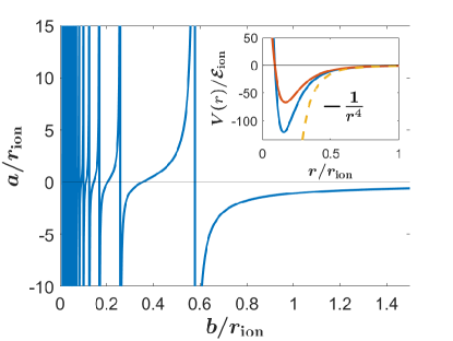
Figure 1: The atom-ion $s$-wave scattering length $a$ as a function of $b$. The inset shows the atom-ion potential for $b/r_{\text{ion}}=0.3$ and 0.35.

Variational ansatz.-

To analyse this challenging interplay between few- and many-body physics, we employ set of a different theoretical techniques. Anticipating the formation of molecular ions involving many bosons bound to ion, we first employ a time-dependent coherent state variational ansatz. In the frame co-moving with the ion, obtained by the unitary transformation $\hat{S}=\exp(-i\hat{\mathbf{r}}\cdot\hat{\mathbf{P}}_{B})$ where $\hat{\mathbf{r}}$ is the position of the ion and $\hat{\mathbf{P}}_{B}=\sum_{\mathbf{k}}\mathbf{k}\hat{\beta}^{\dagger}_{\mathbf{k}}\hat{\beta}_{\mathbf{k}}$ is the total momentum of the atoms Lee et al. (1953), it reads Shashi et al. (2014); Shchadilova et al. (2016)

$$|\Psi(t)\rangle=e^{-i\phi(t)}e^{\sum_{\mathbf{k}}[\gamma_{\mathbf{k}}(t)\hat{\beta}^{\dagger}_{\mathbf{k}}-\gamma^{\ast}_{\mathbf{k}}(t)\hat{\beta}_{\mathbf{k}}]}|\Psi(0)\rangle.$$ (3)

Here, the operator $\hat{\beta}^{\dagger}_{\mathbf{k}}=u_{\mathbf{k}}\hat{b}^{\dagger}_{\mathbf{k}}+v_{\mathbf{k}}\hat{b}_{-\mathbf{k}}$ creates a Bogoliubov mode with momentum ${\mathbf{k}}$ and energy $E_{\mathbf{k}}$. The initial state $|\Psi(0)\rangle=\hat{a}_{\mathbf{k}=0}^{\dagger}|\text{BEC}\rangle$ corresponds to the injection of a zero momentum ion in the BEC.

The Euler-Lagrange equations give the following equations of motion for the parameters $\phi$ and $\gamma_{\mathbf{k}}$ SM

$$\dot{\phi}=-\frac{P_{B}^{2}}{2m}+n_{0}V(\mathbf{0})+\frac{\sqrt{n_{0}}}{2}\sum_{\mathbf{k}}V(\mathbf{k})W_{\mathbf{k}}(\gamma^{\ast}_{\mathbf{k}}+\gamma_{\mathbf{k}}),$$ (4)

$$i\dot{\gamma}_{\mathbf{k}}=\sqrt{n_{0}}V(\mathbf{k})W_{\mathbf{k}}+\left(E_{\mathbf{k}}+\frac{\mathbf{k}^{2}}{2m}+\mathbf{k}\cdot\frac{\mathbf{P}_{B}}{m}\right)\gamma_{\mathbf{k}}$$

$$+\sum_{\mathbf{k^{\prime}}}V(\mathbf{k}^{\prime}-\mathbf{k})C_{\mathbf{k}\mathbf{k^{\prime}}}\gamma_{\mathbf{k^{\prime}}}-\sum_{\mathbf{k^{\prime}}}V(\mathbf{k}^{\prime}+\mathbf{k})\tilde{C}_{\mathbf{k}\mathbf{k^{\prime}}}\gamma_{\mathbf{k^{\prime}}}^{\ast},$$ (5)

where ${\mathbf{P}}_{B}=\sum_{\mathbf{k}}|\gamma_{\mathbf{k}}|^{2}{\mathbf{k}}$, $W_{\mathbf{k}}=\sqrt{\epsilon_{\mathbf{k}}/E_{\mathbf{k}}}$, $C_{\mathbf{k}\mathbf{k^{\prime}}}=u_{\mathbf{k}}u_{\mathbf{k}^{\prime}}+v_{\mathbf{k}}v_{\mathbf{k}}^{\prime}$, $\tilde{C}_{\mathbf{k}\mathbf{k}^{\prime}}=u_{\mathbf{k}}v_{\mathbf{k^{\prime}}}+v_{\mathbf{k}}u_{\mathbf{k^{\prime}}}$, and $u_{\mathbf{k}}^{2}/v_{\mathbf{k}}^{2}=[(\epsilon_{\mathbf{k}}+g_{B}n_{0})/E_{\mathbf{k}}\pm 1]/2$ the usual coherence factors.

We solve Eqs. (4)-(5) numerically, from which the dynamical overlap $S(t)=\langle\Psi(0)|\Psi(t)\rangle=e^{-i\phi(t)}e^{-\frac{1}{2}\sum_{\mathbf{k}}{|\gamma_{\mathbf{k}}|}^{2}}$ with the initial state can be calculated. The impurity spectral function can then be obtained by a Fourier transform $A(\omega)=\text{Re}\int_{0}^{\infty}S(t)e^{i\omega t}dt/\pi$ Knap et al. (2012); SM .

Dressing cloud.-

To further analyse the nature of the many-body states, we use a thermodynamic argument to calculate the number of atoms $\Delta N$ in the dressing cloud around the ion. This gives Massignan et al. (2005); Massignan and Bruun (2011)

$$\Delta N=-{\left(\frac{\partial\mu_{I}}{\partial n_{0}}\right)}{\left(\frac{\partial n_{0}}{\partial\mu_{B}}\right)}_{n_{I}=0}=-{\left(\frac{\partial\mu_{I}}{\partial\mu_{B}}\right)}_{n_{I}=0},$$ (6)

where $\mu_{I}$ is the energy change when the ion is added to the BEC, $\mu_{B}=g_{B}n_{0}$ is the chemical potential of the atoms, and $n_{I}$ is the ion density, which is zero for a single ion. For a given many-body state with energy $\mathcal{E}_{j}$, we set $\mu_{I}=\mathcal{E}_{j}$ in Eq. (6) to calculate $\Delta N$.

Polarons.-

The ion spectral function obtained from the variational ansatz is shown in Fig. 2(top) for a density $n_{0}r_{\text{ion}}^{3}=1$ and zero temperature as a function of $b$ and the corresponding scattering length $a$. For large $b$ meaning weak coupling $1/k_{n}a\ll-1$ with $k_{n}^{3}/6\pi^{2}=n_{0}$, there is a well-defined quasiparticle with mean-field energy $E=2\pi an_{0}/m_{r}$. Its energy decreases with decreasing $b$ (increasing $1/k_{n}a$) corresponding to an increasing depth of the potential, and the mean-field expression eventually breaks down. This quasiparticle is the attractive Bose polaron for the ion in direct analogy with what is observed for neutral impurities Jørgensen et al. (2016); Hu et al. (2016); Peña Ardila et al. (2019); Yan et al. (2020). In the inset of Fig. 2, we see that number of bosons in the dressing cloud around the ion can be quite large reflecting the strength and range of the atom-ion interaction. In the weak coupling limit $b/r_{ion}\gg 1$, we recover the mean-field result $\Delta N=-a/a_{B}$ Massignan et al. (2005). The attractive polaron remains a stable ground state with decreasing $b$ but with a very small residue. Since we have added a small imaginary part to the frequency for numerical reasons, its quasiparticle peak becomes indistinguishable from the many-body continuum starting at energies just above foo .

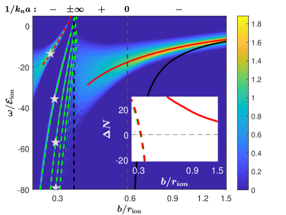
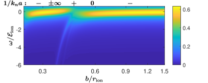
Figure 2: The zero momentum ion spectral function $A(\omega)$ as function of the potential parameter $b$ and the corresponding scattering length $a$ for $n_{0}r_{\text{ion}}^{3}=1$(top) and $n_{0}r_{\text{ion}}^{3}=0.01$ (bottom). The black dashed line is the mean-field energy, the red line is the ladder approximation for the attractive polaron present for $b/r_{\text{ion}}\gtrsim 0.5$, the red dashed line the attractive polaron present for $b/r_{\text{ion}}\lesssim 0.34$, and the green lines are the molecular states obtained from the Bethe-Salpeter equation. The stars $\star$ signify the breakdown of the Bogoliubov approximation. The number of atoms in the dressing cloud is shown in the inset with the same color coding as the main figure.

Figure 2 shows a number of new states that emerge in the regime $b/r_{ion}<0.58$ where the atom-ion interaction supports a two-body bound state. We have $a>0$ for $0.58>b/r_{ion}>0.35$ and $a\leq 0$ for $0.35\geq b/r_{ion}>0.26$ where another bound state emerges, see Fig. 1. Consider first the branch with the highest energy emerging for $b/r_{ion}\simeq 0.34\Rightarrow 1/k_{n}a\simeq-1.45$, highlighted by a red dashed line. Its energy $\varepsilon_{P}$ is larger than zero for $b/r_{ion}\gtrsim 0.32$ where the number of particles $\Delta N$ in its dressing cloud is negative as shown in the inset. From this we conclude that it is a repulsive polaron quasiparticle. Its energy becomes negative for $b/r_{ion}\lesssim 0.32$ where $\Delta N>0$ showing that it smoothly evolves into an attractive polaron with increasing depth of the ion-atom interaction potential. Note that there is no analogue of such an attractive polaron when there is a bound state for a short-range interaction.

Molecular ions.-

Furthermore, Fig. 2 shows several new low energy states emerging together with the repulsive polaron at $b/r_{ion}\lesssim 0.34$. As we will now demonstrate, they arise from the binding of $1,2,\ldots$ bosons to the ion. Consider the scattering matrix between an ion with momentum/energy $k_{1}=(\mathbf{k}_{1},i\omega_{1})$ and an atom with momentum/energy $k_{1}=(\mathbf{k}_{1},i\omega_{1})$. In the ladder approximation, it obeys the Bethe-Salpeter equation SM

$$\Gamma({\mathbf{k}}_{1},{\mathbf{k}}_{2},{\mathbf{q}};i\omega_{1}+i\omega_{2})=V({\mathbf{q}})-\sum_{q^{\prime}}V({\mathbf{q}}^{\prime})G_{11}({k}_{2}-q^{\prime})$$

$$\times G({k}_{1}+q^{\prime})\Gamma(\mathbf{k}_{1}+\mathbf{q}^{\prime},{\mathbf{k}}_{2}-\mathbf{q}^{\prime},\mathbf{q-q}^{\prime};i\omega_{1}+i\omega_{2}),$$ (7)

where ${\mathbf{q}}$ is the momentum transfer, $G({k})=1/(i\omega-{\mathbf{k}}^{2}/2m)$ is the ion Green’s function, and $G_{11}(k)=u^{2}_{\mathbf{k}}/(i\omega-E_{\mathbf{k}})-v^{2}_{\mathbf{k}}/(i\omega+E_{\mathbf{k}})$ is the normal BEC Green’s function for the atoms. The sum $\sum_{q^{\prime}}\equiv T\sum_{i\omega}\int d^{3}q/(2\pi)^{3}$ is both over momenta $\mathbf{q}$ and Matsubara frequencies $i\omega$, and we analytically continue $i\omega\rightarrow\omega+i0_{+}$ as usual. Due to the long range of the atom-ion potential, it is essential to retain its full momentum dependence in Eq. (7), in contrast to the usual case of a short-range interaction between neutral atoms.

The ion self-energy $\Sigma({\mathbf{k}},\omega)=n_{0}\Gamma({\mathbf{k}},0,0;\omega)$ describes the scattering of a single atom out of the BEC, and the quasiparticle energy is obtained by solving $\varepsilon_{P,\mathbf{k}}=k^{2}/2m+\Sigma({\mathbf{k}},\varepsilon_{P,\mathbf{k}})$. The resulting ladder approximation has successfully been applied to explain experimental results for neutral impurities in a BEC forming Bose polarons Rath and Schmidt (2013); Jørgensen et al. (2016); Hu et al. (2016); Peña Ardila et al. (2019); Yan et al. (2020). In the present case it yields the red line in Fig. 2, which agrees very well with the variational result for the attractive polaron stable, whereas it fails to capture the lower lying states.

This can however be addressed by noting that a possible pole of the zero momentum scattering matrix gives the energy of a bound state. Thus, by replacing in Eq. (7) the bare ion Green’s function with the polaron Green’s function $G_{j}({k})=1/(i\omega-\varepsilon_{P}-{\mathbf{k}}^{2}/2m)$ will give the energy of a possible dimer consisting of an atom bound to the polaron. This yields the top green line in Fig. 2. The excellent agreement with the variational ansatz show that this state indeed arises from the binding of an atom to the ion. We perform this procedure recursively by calculating the scattering matrix between this new molecular state and an atom, which then yields the second green line below the attractive polaron in Fig. 2 and so on. Since energies obtained from this procedure agree very well with those from the variational ansatz, we conclude that these branches involve the binding of one, two, $\ldots$ atoms to the ion. In the following, we refer for brevity to these states as molecular ions although they do have a non-zero quasiparticle residue as is evident from Fig. 2. We note that dimer states consisting of one atom bound to the ion have recently been observed Dieterle et al. (2020b), and our prediction of molecular states involving more atoms is consistent with earlier results based on different methods Côté et al. (2002); Massignan et al. (2005); Schurer et al. (2017); Astrakharchik et al. (2020).

Note that these molecules are stable only for $b$ significantly smaller than $b/r_{ion}=0.58$ where the two-body atom-ion state emerges. Hence, many-body effects destabilize the binding of atoms to the ion as compared to the vacuum case. The molecules are stable for $a>0$ and $a<0$ as opposed to the case of a short-range interaction, where similar states are predicted to exist only for $a<0$ Shchadilova et al. (2016).

The binding of additional atoms to the ion will eventually be halted by the repulsion between them giving a positive energy $\sim a_{B}\Delta N^{2}$. While this effect is not included in our theory, we can estimate when it becomes important by calculating the gas factor of the dressing cloud $\sqrt{n_{\text{cl}}a_{B}^{3}}$. Here, $n_{\text{cl}}=\Delta N/\bar{r}^{3}$ is the average density of atoms in the dressing cloud with $\bar{r}=[\int\!d^{3}rr^{2}|\phi({\mathbf{r}})|^{2}]^{1/2}$ the spatial size of the molecule with wave function $\phi({\mathbf{r}})$. As explicitly shown in the Supp. Mat. SM , the size of the molecular states is $\sim r_{\text{ion}}$ and decreases as they becomes increasingly bound. The $\star$’s in Fig. 2 indicate when the gas factor of a given molecular state becomes larger than $0.1$. A reliable description of this region requires one to go beyond Bogoliubov theory.

Simplified model.-

The basic physics of the binding of bosons to the ion can be described using the Hamiltonian

$$\hat{H}_{s}=\sum_{l=0}^{\infty}\left\{[\varepsilon_{P}+\varepsilon_{B}(l-1)]\hat{c}_{l}^{\dagger}\hat{c}_{l}+g\sqrt{n_{0}}\hat{c}_{l+1}^{\dagger}\hat{c}_{l}+\text{h.c.}\right\}.$$ (8)

Here, $\hat{c}_{l}$ creates a state with $l$ bosons bound the polaron, $\varepsilon_{B}<0$ is the energy released by the binding of a boson, and $g\sqrt{n_{0}}$ is the matrix element for this process. Note that this is proportional to $\sqrt{n_{0}}$ since the boson is taken from the BEC with density $n_{0}$. This also means that we can suppress the momentum since this is zero for all states. The model is easily solved giving a continued fraction form of the zero momentum ion Green’s function

$$G(\omega)^{-1}=\omega-\varepsilon_{P}-\cfrac{g^{2}n_{0}}{\omega-\varepsilon_{B}-\cfrac{g^{2}n_{0}}{\omega-2\varepsilon_{B}-\cfrac{g^{2}n_{0}}{\omega-3\varepsilon_{B}-\ldots}}}.$$ (9)

For $g^{2}n_{0}/\varepsilon_{B}^{2}\ll 1$, the highest energy pole is $\simeq\varepsilon_{P}$ corresponding to the repulsive polaron and there is an infinite ladder of poles with energies $\simeq\varepsilon_{P}-l\varepsilon_{B}$ corresponding to states with $l=1,2,\ldots$ bosons bound to the ion. The residue of these states is $(g^{2}n_{0}/\varepsilon_{B}^{2})^{l}\propto n_{0}^{l}$ reflecting that they involve $l$ bosons taken from the BEC. This scaling explains the decreasing spectral weight of the deeper molecular lines seen Fig. 2.

It also means that the relative spectral weight of the different lines depends on the BEC density. This is illustrated in Fig. 2(bottom), which shows the ion spectral function for $n_{0}r_{\text{ion}}^{3}=0.01$. We see that only two states with significant spectral weight emerge for $b/r_{ion}<0.58$ when the atom-ion potential supports a bound state: The new polaron and the highest molecular state with one boson bound to the ion. Since the ground state remains the attractive polaron, this is consistent with the finding that for a static ion in the dilute limit, there are $2\nu_{s}+1$ solutions to the Gross-Pitaevskii equation where $\nu_{s}$ is the number of two-body bound states of the atom-ion interaction potential Massignan et al. (2005); Pie . The small spectral weight of the bound states involving more than one boson also means that they are quite sensitive to additional damping.

Dynamics.-

We finally investigate the quantum dynamics after a zero momentum ion is injected in the BEC. The dynamical overlap $S(t)=\langle\Psi(0)|\Psi(t)\rangle$ is plotted in Fig. 3. For $b/r_{ion}=2$, we have $|S(t)|\rightarrow Z$ for $t\rightarrow\infty$ where $Z$ is the quasiparticle residue of the attractive polaron Shchadilova et al. (2016); Nielsen et al. (2019). For $b/r_{ion}=0.5$ on the other hand, $S(t)$ decreases monotonically to zero since there is no well-defined quasiparticle, see Fig. 2. In the right panel of Fig. 3, we plot $S(t)$ when the molecular states are present. For $b/r_{ion}=0.3$ (orange), $S(t)$ oscillates with an almost constant amplitude after an initial decay. These oscillations arise from a coherent population of the molecular states and the polaron, see Fig. 2. For $b/r_{ion}=0.25$ (blue) on the other hand, the polaron is strongly damped giving rise to decoherence and $S(t)$ therefore decays monotonically to zero, see Fig. 2.

Figure 3 shows that the many-body time-scale is $\tau_{\text{ion}}\approx 1/\mathcal{E}_{\text{ion}}=13.5\mu\text{s}$ for $r_{\text{ion}}=100\text{nm}$. This should be compared to the three-body recombination time $\tau_{\text{3B}}=1/K_{3}n_{0}^{2}$. Taking $K_{3}\approx 3.3-6\times 10^{25}\text{cm}^{6}/\text{s}$ Härter et al. (2012b); Dieterle et al. (2020a) and $n_{0}=10^{14}\text{cm}^{-3}$ for a typical BEC yields $\tau_{\text{3B}}\approx 160-300\mu\text{s}$, showing that the many-body phenomena described here should be observable before three-body decay sets in.

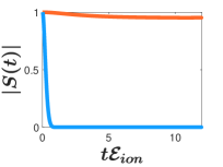
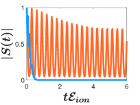
Figure 3: In the left panel $|S(t)|$ is shown for $b/r_{ion}=2$ (orange) and $b/r_{ion}=0.5$ (blue). The right panel shows $|S(t)|$ for $b/r_{ion}=0.3$ (orange) and $b/r_{ion}=0.25$ (blue).

Conclusions and outlook.- Using several theoretical methods, we studied the static and dynamical properties of a mobile ion in a BEC. The long-range nature of the atom-ion interaction was shown to result in a rich spectrum with several quasiparticle and molecular states. We demonstrated that the quantum dynamics after a quench where the ion is injected into the BEC is characterised by coherent oscillations between the different states as well as decay. Our work demonstrates the diverse and exciting physics that can be realised in ion-atom systems and motivates future investigations into these hybrid systems. In particular, dimer states consisting of one atom bound to the ion have recently been observed, and it would be very interesting to extend this experimental search to the predicted deeper lying larger molecular ions preferably using a high density BEC Dieterle et al. (2020b). Also, radio-frequency and Ramsey spectroscopy have been used to measure the spectral function and the dynamics for neutral impurities in a BEC Jørgensen et al. (2016); Hu et al. (2016); Peña Ardila et al. (2019); Yan et al. (2020); Skou et al. (2020), and analogous probes for charged impurities should be highly useful.

Acknowledgments.- We acknowledge financial support from the Villum Foundation, the Independent Research Fund Denmark-Natural Sciences via Grant No. DFF -8021-00233B, and US Army CCDC Atlantic Basic and Applied Research via grant W911NF-19-1-0403. We thank P. Massignan for very useful comments, and T. Pohl and K. Mølmer for discussions.

I Supplemental Material

I.1 Equations of motion

The Hamiltonian in Eq. [1] (main text) written explicitly in terms of the position $\hat{\mathbf{r}}$ and momentum $\hat{\mathbf{P}}$ operators of the ion reads

$$\hat{H}=\frac{\hat{\mathbf{P}}^{2}}{2m}+\sum_{\mathbf{k}}\epsilon_{\mathbf{k}}\hat{b}^{\dagger}_{\mathbf{k}}\hat{b}_{\mathbf{k}}+\frac{g_{B}}{2}\sum_{\mathbf{k},\mathbf{k^{\prime}},\mathbf{q}}\hat{b}^{\dagger}_{\mathbf{k^{\prime}+q}}\hat{b}^{\dagger}_{\mathbf{k-q}}\hat{b}_{\mathbf{k^{\prime}}}\hat{b}_{\mathbf{k}}+\sum_{\mathbf{k},\mathbf{q}}V(\mathbf{q})e^{-i\mathbf{q}\cdot\hat{\mathbf{r}}}\hat{b}^{\dagger}_{\mathbf{k+q}}\hat{b}_{\mathbf{k}}.$$ (10)

We perform the following Bogoliubov transformation

$$\hat{\beta}_{\mathbf{k}}=u_{\mathbf{k}}\hat{b}_{\mathbf{k}}-v_{\mathbf{k}}\hat{b}_{\mathbf{-k}}^{\dagger},\ \hat{\beta}_{\mathbf{k}}^{\dagger}=u_{\mathbf{k}}\hat{b}_{\mathbf{k}}^{\dagger}-v_{\mathbf{k}}\hat{b}_{\mathbf{-k}},$$ (11)

where $\mathbf{k}\neq\mathbf{0},$ and under the standard Bogoliubov approximations we arrive at an extended Fröhlich Hamiltonian that takes the form

$$\hat{H}=\frac{\hat{\mathbf{P}}^{2}}{2m}+n_{0}V(\mathbf{0})+\sum_{\mathbf{k\neq\mathbf{0}}}\omega_{\mathbf{k}}\hat{\beta}^{\dagger}_{\mathbf{k}}\hat{\beta}_{\mathbf{k}}+\sqrt{n_{0}}\sum_{\mathbf{q}}\sqrt{\epsilon_{\mathbf{q}}/\omega_{\mathbf{q}}}V(\mathbf{q})e^{-i\mathbf{q}\cdot\hat{\mathbf{r}}}\left(\hat{\beta}_{\mathbf{q}}^{\dagger}+\hat{\beta}_{\mathbf{-q}}\right)$$ (12)

$$+\sum_{\mathbf{k}\mathbf{k^{\prime}}}V(\mathbf{k}-\mathbf{k}^{\prime})e^{i(\mathbf{k^{\prime}}-\mathbf{k})\cdot\hat{\mathbf{r}}}(u_{\mathbf{k^{\prime}}}u_{\mathbf{k}}+v_{\mathbf{k^{\prime}}}v_{\mathbf{k}})\hat{\beta}^{\dagger}_{\mathbf{k}}\hat{\beta}_{\mathbf{k^{\prime}}}$$

$$-\sum_{\mathbf{k}\mathbf{k^{\prime}}}V(\mathbf{k}^{\prime}+\mathbf{k})e^{-i(\mathbf{k}+\mathbf{k}^{\prime})\cdot\hat{\mathbf{r}}}(v_{\mathbf{k^{\prime}}}u_{\mathbf{k}}+u_{\mathbf{k^{\prime}}}v_{\mathbf{k}})(\hat{\beta}_{\mathbf{k}}^{\dagger}\hat{\beta}_{\mathbf{k^{\prime}}}^{\dagger}+\hat{\beta}_{-\mathbf{k}}\hat{\beta}_{\mathbf{-k^{\prime}}}).$$

It is convenient to employ the following canonical transformation

$$\hat{S}=e^{-i\hat{\mathbf{r}}\cdot\hat{\mathbf{P}}_{B}}=e^{-i\hat{\mathbf{r}}\cdot\sum_{\mathbf{k}}\mathbf{k}\beta^{\dagger}_{\mathbf{k}}\beta_{\mathbf{k}}},$$ (13)

since the transformation eliminates the coordinates of the ion and the operator $\hat{\mathbf{P}}$ commutes with the final form of the Hamiltonian:

$$\hat{\mathcal{H}}=\hat{S}^{-1}\hat{H}\hat{S}=\frac{(\hat{\mathbf{P}}-\hat{\mathbf{P}}_{B})^{2}}{2m}+n_{0}V(\mathbf{0})+\sum_{\mathbf{k\neq\mathbf{0}}}\omega_{\mathbf{k}}\hat{\beta}^{\dagger}_{\mathbf{k}}\hat{\beta}_{\mathbf{k}}+\sqrt{n_{0}}\sum_{\mathbf{q}}\sqrt{\epsilon_{\mathbf{q}}/\omega_{\mathbf{q}}}V(\mathbf{q})\left(\hat{\beta}_{\mathbf{q}}^{\dagger}+\hat{\beta}_{\mathbf{-q}}\right)$$ (14)

$$+\sum_{\mathbf{k}\mathbf{k^{\prime}}}V(\mathbf{k}-\mathbf{k}^{\prime})(u_{\mathbf{k^{\prime}}}u_{\mathbf{k}}+v_{\mathbf{k^{\prime}}}v_{\mathbf{k}})\hat{\beta}^{\dagger}_{\mathbf{k}}\hat{\beta}_{\mathbf{k^{\prime}}}-\sum_{\mathbf{k}\mathbf{k^{\prime}}}V(\mathbf{k}^{\prime}+\mathbf{k})(v_{\mathbf{k^{\prime}}}u_{\mathbf{k}}+u_{\mathbf{k^{\prime}}}v_{\mathbf{k}})(\hat{\beta}_{\mathbf{k}}^{\dagger}\hat{\beta}_{\mathbf{k^{\prime}}}^{\dagger}+\hat{\beta}_{-\mathbf{k}}\hat{\beta}_{\mathbf{-k^{\prime}}}).$$

From the ansatz $|\Psi(t)\rangle=\exp(-i\phi(t))\hat{\mathcal{O}}|\Psi(0)\rangle$ we derive the equations of motion applying a time-dependent variational principle from the Euler-Lagrange equations

$$\frac{d}{dt}\frac{\partial L}{\partial\dot{f}}-\frac{\partial L}{\partial f}=0,$$ (15)

where $\hat{\mathcal{O}}=e^{\sum_{\mathbf{k}}(\gamma_{\mathbf{k}}(t)\hat{\beta}^{\dagger}_{\mathbf{k}}-\gamma^{\ast}_{\mathbf{k}}(t)\hat{\beta}_{\mathbf{k}})}$ and $f=\{\gamma,\gamma^{*}\}.$ Here, the Lagrangian is given by

$$L=\langle\Psi|i\partial_{t}-\hat{\mathcal{H}}|\Psi\rangle=i\langle\Psi|\partial_{t}|\Psi\rangle-\langle\Psi|\hat{\mathcal{H}}|\Psi\rangle.$$ (16)

After some algebra, we obtain the equations of motion for $\phi(t)$ and $\gamma(t)$ given in the main text (Eqs. [4] and [5]).

I.2 Numerical procedure: Variational Ansatz

We solve the equations of motions in Eqs. [4] and [5] (main text) by discretising the $\mathbf{k}$-space, this allows us to re-write the equations of motions for $\gamma$ as a finite system of equation of motions, which can be written in a matrix form Dzsotjan et al. (2020),

$$i\dot{\bm{\gamma}}=A\bm{\gamma}+\mathbf{K},$$ (17)

where $\bm{\gamma}=d/dt(\gamma_{1},\ldots,\gamma_{N_{\text{max}}},\gamma_{1}^{\ast},\ldots,\gamma_{N_{\text{max}}}^{\ast})$, $A$ is matrix that contains all the coefficients describing the system of equations, and $\mathbf{K}$ is a constant vector with the constant terms in the equations of motion. The solution is given by

$$\bm{\gamma}=\exp(-iAt)\mathbf{d}-A^{-1}\mathbf{K},$$ (18)

where $\mathbf{d}$ is a vector that is determined from the initial condition. In our case $\bm{\gamma}(0)=\mathbf{0}$ and thus $\mathbf{d}=A^{-1}\mathbf{K}$. Once the coefficients $\gamma_{\mathbf{k}}$ are obtained, we obtain the dynamics of $\phi$.

To numerically resolve the spectral function from the Fourier transform of the dynamical overlap, we multiply the latter by an exponential decay $S(t)\rightarrow S(t)e^{-\delta t}$, this procedure is equivalent to adding an artificial broadening to the spectral function. For our numerical calculations we take $\delta=0.5$. Finally, due to the finite size of the time interval, we correct the spectral function to maintain a positive value of $A(\omega)$ Dishan (1995).

I.3 $T$-matrix approach and few-body phonon states

Since the potential is frequency independent one can perform the Matsubara sum in Eq. [7] (main text) to arrive to the following Bethe-Salpeter equation

$$\Gamma(\mathbf{k},\mathbf{Q}-\mathbf{k},\mathbf{k}-\mathbf{k}^{\prime},\Omega)=V(\mathbf{k}-\mathbf{k}^{\prime})+\int\frac{d^{3}\mathbf{q}}{(2\pi)^{3}}V(\mathbf{k}-\mathbf{q})\Pi_{\mathbf{q}}(\mathbf{Q},\Omega)\Gamma(\mathbf{q},\mathbf{Q}-\mathbf{q},\mathbf{q}-\mathbf{k}^{\prime},\Omega),$$ (19)

that describes the interaction between a boson and an ion that scatters from states with momentum-energy $k=(\mathbf{k},\omega)$ and $Q-k=(\mathbf{Q}-\mathbf{k},\Omega-\omega)$ into states $k^{\prime}=(\mathbf{k}^{\prime},\omega^{\prime})$ and $Q-k^{\prime}=(\mathbf{Q}-\mathbf{k}^{\prime},\Omega-\omega^{\prime}).$ Here the propagator $\Pi_{\mathbf{q}}(\mathbf{Q},\Omega)$ is given at zero-temperature by

$$\Pi_{\mathbf{q}}(\mathbf{Q},\Omega)=\frac{u_{\mathbf{Q}/2-\mathbf{q}}^{2}}{\omega-\epsilon^{I}_{\mathbf{Q}/2+\mathbf{q}}-E_{\mathbf{Q}/2-\mathbf{q}}}$$ (20)

= +

Figure 4: Scattering matrix $\mathcal{T}$ for the ion-boson potential, the solid red lines correspond to the BEC Green’s function, while the blue denote the ion propagator. The wavy line depicts the boson-ion interaction potential $V(\mathbf{q})$.

We focus on the low-energy scattering of the Bethe-Salpeter equation in Fig. 4, thus we take $k=k^{\prime}=0$, and $\mathbf{Q}=0$ and simplify the notation for this scattering process by defining $\Gamma_{0}(\omega)$. We take a quasiparticle approach to study the ionic impurity dressed by the Bogoliubov excitations,

$$\Sigma(\omega)=n_{B}\Gamma_{0}(\omega),$$ (21)

and calculate the dressed impurity Green’s function given by

$$G_{I}(\mathbf{p},\omega)=\frac{1}{\omega-\epsilon_{\mathbf{p}}^{I}-\Sigma(p,\omega)},$$ (22)

here the poles of $G_{I}$ determine the quasiparticle energy, which can be obtained by solving self-consistently the following equation $\omega-\Sigma(\omega)=0.$

To determine the few-body states of many-phonons bound to the ion, we solve recursively the scattering the $T$-matrix by replacing the ion dispersion by the immediate upper polaron branch, that is, to solve the Bethe-Salpeter equation we take

$$\Pi_{\mathbf{q}}(\mathbf{Q},\Omega)\rightarrow\frac{u_{\mathbf{Q}/2-\mathbf{q}}^{2}}{\omega-E^{P,i}_{\mathbf{Q}/2+\mathbf{q}}-E_{\mathbf{Q}/2-\mathbf{q}}},$$ (23)

where $E^{P,i}$ denotes the polaron energy of the $i$-th upper branch.

I.4 Molecular radius

Fig. 5 shows that the size of the highest molecular state (the repulsive polaron with one Bogoliubov phonon bound) decreases as it becomes increasingly bound with increasing $1/k_{n}a$, as expected. For identical binding energy, the different molecular states will have the same radius. We can therefore calculate the gas factor for each molecular state and estimate at which interaction the Bogoliubov theory is no longer valid.

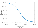
Figure 5: The spatial size of the highest molecular state as function of $1/k_{n}a$. As the interaction is increased, the molecular size decreases.

References

- Bloch et al. (2008) Immanuel Bloch, Jean Dalibard, and Wilhelm Zwerger, “Many-body physics with ultracold gases,” Rev. Mod. Phys. 80, 885–964 (2008).
- Bloch et al. (2012) Immanuel Bloch, Jean Dalibard, and Sylvain Nascimbene, “Quantum simulations with ultracold quantum gases,” Nature Physics 8, 267–276 (2012).
- Yarmchuk et al. (1979) E. J. Yarmchuk, M. J. V. Gordon, and R. E. Packard, “Observation of stationary vortex arrays in rotating superfluid helium,” Phys. Rev. Lett. 43, 214–217 (1979).
- Meyer and Reif (1958) Lothar Meyer and F. Reif, “Mobilities of he ions in liquid helium,” Phys. Rev. 110, 279–280 (1958).
- Atkins (1959) K. R. Atkins, “Ions in liquid helium,” Phys. Rev. 116, 1339–1343 (1959).
- Gross (1962) E.P Gross, “Motion of foreign bodies in boson systems,” Annals of Physics 19, 234 – 253 (1962).
- Ahonen et al. (1976) A. I. Ahonen, J. Kokko, O. V. Lounasmaa, M. A. Paalanen, R. C. Richardson, W. Schoepe, and Y. Takano, “Mobility of negative ions in superfluid ,” Phys. Rev. Lett. 37, 511–515 (1976).
- Roach et al. (1977) Paul D. Roach, J. B. Ketterson, and Pat R. Roach, “Mobility of positive and negative ions in superfluid ,” Phys. Rev. Lett. 39, 626–629 (1977).
- Ahonen et al. (1978) A. I. Ahonen, J. Kokko, M. A. Paalanen, R. C. Richardson, W. Schoepe, and Y. Takano, “Negative ion motion in normal and superfluid 3he,” Journal of Low Temperature Physics 30, 205–228 (1978).
- Salomaa et al. (1980) M. Salomaa, C. J. Pethick, and Gordon Baym, “Mobility tensor of the electron bubble in superfluid -,” Phys. Rev. Lett. 44, 998–1001 (1980).
- Baym et al. (1979) Gordon Baym, C. J. Pethick, and M. Salomaa, “Mobility of negative ions in superfluid 3he-b,” Journal of Low Temperature Physics 36, 431–466 (1979).
- Grier et al. (2009) Andrew T. Grier, Marko Cetina, Fedja Oručević, and Vladan Vuletić, “Observation of cold collisions between trapped ions and trapped atoms,” Phys. Rev. Lett. 102, 223201 (2009).
- Zipkes et al. (2010) Christoph Zipkes, Stefan Palzer, Carlo Sias, and Michael Köhl, “A trapped single ion inside a bose–einstein condensate,” Nature 464, 388–391 (2010).
- Härter et al. (2012a) Arne Härter, Artjom Krükow, Andreas Brunner, Wolfgang Schnitzler, Stefan Schmid, and Johannes Hecker Denschlag, “Single ion as a three-body reaction center in an ultracold atomic gas,” Phys. Rev. Lett. 109, 123201 (2012a).
- Ratschbacher et al. (2012) Lothar Ratschbacher, Christoph Zipkes, Carlo Sias, and Michael Köhl, “Controlling chemical reactions of a single particle,” Nature Physics 8, 649–652 (2012).
- Kleinbach et al. (2018) K. S. Kleinbach, F. Engel, T. Dieterle, R. Löw, T. Pfau, and F. Meinert, “Ionic impurity in a bose-einstein condensate at submicrokelvin temperatures,” Phys. Rev. Lett. 120, 193401 (2018).
- Sikorsky et al. (2018) Tomas Sikorsky, Ziv Meir, Ruti Ben-shlomi, Nitzan Akerman, and Roee Ozeri, “Spin-controlled atom–ion chemistry,” Nature Communications 9, 920 (2018).
- Feldker et al. (2020) T. Feldker, H. Fürst, H. Hirzler, N. V. Ewald, M. Mazzanti, D. Wiater, M. Tomza, and R. Gerritsma, “Buffer gas cooling of a trapped ion to the quantum regime,” Nature Physics 16, 413–416 (2020).
- Schmidt et al. (2020) J. Schmidt, P. Weckesser, F. Thielemann, T. Schaetz, and L. Karpa, “Optical traps for sympathetic cooling of ions with ultracold neutral atoms,” Phys. Rev. Lett. 124, 053402 (2020).
- Dieterle et al. (2020a) Thomas Dieterle, Moritz Berngruber, Christian Hölzl, Robert Löw, Krzysztof Jachymski, Tilman Pfau, and Florian Meinert, “Transport of a single cold ion immersed in a bose-einstein condensate,” (2020a), arXiv:2007.00309 [physics.atom-ph] .
- Dieterle et al. (2020b) T. Dieterle, M. Berngruber, C. Hölzl, R. Löw, K. Jachymski, T. Pfau, and F. Meinert, “Inelastic collision dynamics of a single cold ion immersed in a bose-einstein condensate,” Phys. Rev. A 102, 041301 (2020b).
- Casteels et al. (2011) W. Casteels, J. Tempere, and J. T. Devreese, “Polaronic properties of an ion in a bose-einstein condensate in the strong-coupling limit,” Journal of Low Temperature Physics 162, 266–273 (2011).
- Gao (2010) Bo Gao, “Universal properties in ultracold ion-atom interactions,” Phys. Rev. Lett. 104, 213201 (2010).
- Krükow et al. (2016) Artjom Krükow, Amir Mohammadi, Arne Härter, Johannes Hecker Denschlag, Jesús Pérez-Ríos, and Chris H. Greene, “Energy scaling of cold atom-atom-ion three-body recombination,” Phys. Rev. Lett. 116, 193201 (2016).
- Côté et al. (2002) R. Côté, V. Kharchenko, and M. D. Lukin, “Mesoscopic molecular ions in bose-einstein condensates,” Phys. Rev. Lett. 89, 093001 (2002).
- Massignan et al. (2005) P. Massignan, C. J. Pethick, and H. Smith, “Static properties of positive ions in atomic bose-einstein condensates,” Phys. Rev. A 71, 023606 (2005).
- Schurer et al. (2017) J. M. Schurer, A. Negretti, and P. Schmelcher, “Unraveling the structure of ultracold mesoscopic collinear molecular ions,” Phys. Rev. Lett. 119, 063001 (2017).
- Astrakharchik et al. (2020) G. E. Astrakharchik, L. A. Peña Ardila, R. Schmidt, K. Jachymski, and A. Negretti, “Ionic polaron in a bose-einstein condensate,” (2020), arXiv:2005.12033 [cond-mat.quant-gas] .
- Tomza et al. (2019) Michał Tomza, Krzysztof Jachymski, Rene Gerritsma, Antonio Negretti, Tommaso Calarco, Zbigniew Idziaszek, and Paul S. Julienne, “Cold hybrid ion-atom systems,” Rev. Mod. Phys. 91, 035001 (2019).
- Krych and Idziaszek (2015) Michał Krych and Zbigniew Idziaszek, “Description of ion motion in a paul trap immersed in a cold atomic gas,” Phys. Rev. A 91, 023430 (2015).
- Lee et al. (1953) T. D. Lee, F. E. Low, and D. Pines, “The motion of slow electrons in a polar crystal,” Phys. Rev. 90, 297–302 (1953).
- Shashi et al. (2014) Aditya Shashi, Fabian Grusdt, Dmitry A. Abanin, and Eugene Demler, “Radio-frequency spectroscopy of polarons in ultracold bose gases,” Phys. Rev. A 89, 053617 (2014).
- Shchadilova et al. (2016) Yulia E. Shchadilova, Richard Schmidt, Fabian Grusdt, and Eugene Demler, “Quantum dynamics of ultracold bose polarons,” Phys. Rev. Lett. 117, 113002 (2016).
- (34) See Supplemental Material online for details.
- Knap et al. (2012) Michael Knap, Aditya Shashi, Yusuke Nishida, Adilet Imambekov, Dmitry A. Abanin, and Eugene Demler, “Time-dependent impurity in ultracold fermions: Orthogonality catastrophe and beyond,” Phys. Rev. X 2, 041020 (2012).
- Massignan and Bruun (2011) P. Massignan and G.M. Bruun, “Repulsive polarons and itinerant ferromagnetism in strongly polarized fermi gases,” EPJ D 65, 83–89 (2011).
- Jørgensen et al. (2016) Nils B. Jørgensen, Lars Wacker, Kristoffer T. Skalmstang, Meera M. Parish, Jesper Levinsen, Rasmus S. Christensen, Georg M. Bruun, and Jan J. Arlt, “Observation of attractive and repulsive polarons in a bose-einstein condensate,” Phys. Rev. Lett. 117, 055302 (2016).
- Hu et al. (2016) Ming-Guang Hu, Michael J. Van de Graaff, Dhruv Kedar, John P. Corson, Eric A. Cornell, and Deborah S. Jin, “Bose polarons in the strongly interacting regime,” Phys. Rev. Lett. 117, 055301 (2016).
- Peña Ardila et al. (2019) L. A. Peña Ardila, N. B. Jørgensen, T. Pohl, S. Giorgini, G. M. Bruun, and J. J. Arlt, “Analyzing a bose polaron across resonant interactions,” Phys. Rev. A 99, 063607 (2019).
- Yan et al. (2020) Zoe Z. Yan, Yiqi Ni, Carsten Robens, and Martin W. Zwierlein, “Bose polarons near quantum criticality,” Science 368, 190–194 (2020), https://science.sciencemag.org/content/368/6487/190.full.pdf .
- (41) In the top panel of Fig. 2, we take the logarithm to the spectral function, which visualy makes the width appear larger.
- Rath and Schmidt (2013) Steffen Patrick Rath and Richard Schmidt, “Field-theoretical study of the bose polaron,” Phys. Rev. A 88, 053632 (2013).
- (43) We thank P. Massignan for pointing this result out for us.
- Nielsen et al. (2019) K Knakkergaard Nielsen, L A Peña Ardila, G M Bruun, and T Pohl, “Critical slowdown of non-equilibrium polaron dynamics,” New Journal of Physics 21, 043014 (2019).
- Härter et al. (2012b) Arne Härter, Artjom Krükow, Andreas Brunner, Wolfgang Schnitzler, Stefan Schmid, and Johannes Hecker Denschlag, “Single ion as a three-body reaction center in an ultracold atomic gas,” Phys. Rev. Lett. 109, 123201 (2012b).
- Skou et al. (2020) Magnus G. Skou, Thomas G. Skov, Nils B. Jørgensen, Kristian K. Nielsen, Arturo Camacho-Guardian, Thomas Pohl, Georg M. Bruun, and Jan J. Arlt, “Non-equilibrium dynamics of quantum impurities,” arXiv e-prints , arXiv:2005.00424 (2020), arXiv:2005.00424 [cond-mat.quant-gas] .
- Dzsotjan et al. (2020) David Dzsotjan, Richard Schmidt, and Michael Fleischhauer, “Dynamical variational approach to bose polarons at finite temperatures,” Phys. Rev. Lett. 124, 223401 (2020).
- Dishan (1995) Huang Dishan, “Phase error in fast fourier transform analysis,” Mechanical Systems and Signal Processing 9, 113 – 118 (1995).