Detectability of biosignatures on LHS 1140 b

Abstract

Context. Terrestrial extrasolar planets around low-mass stars are prime targets when searching for atmospheric biosignatures with current and near-future telescopes. The habitable-zone Super-Earth LHS 1140 b could hold a hydrogen-dominated atmosphere and is an excellent candidate for detecting atmospheric features.

Aims. In this study, we investigate how the instellation and planetary parameters influence the atmospheric climate, chemistry, and spectral appearance of LHS 1140 b. We study the detectability of selected molecules, in particular potential biosignatures, with the upcoming James Webb Space Telescope (JWST) and Extremely Large Telescope (ELT).

Methods. In a first step we use the coupled climate-chemistry model, 1D-TERRA, to simulate a range of assumed atmospheric chemical compositions dominated by molecular hydrogen (H₂) and carbon dioxide (CO₂). Further, we vary the concentrations of methane (CH₄) by several orders of magnitude. In a second step we calculate transmission spectra of the simulated atmospheres and compare them to recent transit observations. Finally, we determine the observation time required to detect spectral bands with low resolution spectroscopy using JWST and the cross-correlation technique using ELT.

Results. In H₂-dominated and CH₄-rich atmospheres oxygen (O₂) has strong chemical sinks, leading to low concentrations of O₂ and ozone (O₃). The potential biosignatures ammonia (NH₃), phosphine (PH₃), chloromethane (CH₃Cl) and nitrous oxide (N₂O) are less sensitive to the concentration of H₂, CO₂ and CH₄ in the atmosphere. In the simulated H₂-dominated atmosphere the detection of these gases might be feasible within 20 to 100 observation hours with ELT or JWST, when assuming weak extinction by hazes.

Conclusions. If further observations of LHS 1140 b suggest a thin, clear, hydrogen-dominated atmosphere, the planet would be one of the best known targets to detect biosignature gases in the atmosphere of a habitable-zone rocky exoplanet with upcoming telescopes.

1 Introduction

The nearby temperate Super-Earth LHS 1140 b (Dittmann et al., 2017; Ment et al., 2019) is an exciting target for atmospheric characterization. Morley et al. (2017) assumed Venus, Titan and Earth-like atmospheres for LHS 1140 b. Their results suggest that atmospheric characterization with the James Webb Space Telescope (JWST) could be possible although challenging.

A recent study of the temporal radiation environment of the LHS 1140 system suggests that the planet receives relatively constant near ultraviolet (NUV) (177-283 nm) flux ¡2% compared to that of Earth (Spinelli et al., 2019). The results of Chen et al. (2019) suggest that LHS 1140 b might be stable against complete ocean desiccation due to the low UV activity of the host star, which would bode well for its habitability. However, Chen et al. (2019) assumed a rather low UV flux for the star which might lead to an underestimation of the water loss. Further, due to the extended pre-main sequence phase of M dwarfs (see e.g. Baraffe et al., 2015; Luger & Barnes, 2015) LHS 1140 b may have experienced extreme water loss before the star entered the main sequence phase (see e.g. Luger & Barnes, 2015).

Assuming an Earth-like atmosphere with updated sea-ice paramerization the 3D model study of Yang et al. (2020) suggested a reduced surface ocean on LHS 1140 b (from 12% to 3% surface coverage). Diamond-Lowe et al. (2020) observed two transits of LHS 1140 b with the twin Magellan Telescopes but their analysis suggested that a precision increased by a factor of about 4 was needed for the detection of e.g. a cloudless hydrogen atmosphere present at amounts consistent with the bulk density. Recently, Edwards et al. (2020) presented spectrally resolved observations of LHS 1140 b using the G141 grism of the Wide Field Camera 3 (WFC3) on the Hubble Space Telescope (HST). Their results suggest that the planet may host a clear H₂-dominated atmosphere and show evidence of an absorption feature at 1.4 $\mu$m.

The processes affecting climate and composition of Super-Earths, such as LHS 1140 b are not well known. Evidence was found that there is a dip in the radius distribution of extrasolar planets at 1.5–2.0 $R_{\oplus}$ (see e.g. Owen & Wu, 2013; Fulton et al., 2017; Van Eylen et al., 2018; Hardegree-Ullman et al., 2020). With a radius of $\sim$1.7 $R_{\oplus}$ LHS 1140 b lies within this so called ’Radius Valley’ (Ment et al., 2019), which is interpreted as the transition between predominantly rocky planets and volatile-rich planets. A number of studies have investigated the origin of the Radius Valley (see e.g. Owen & Wu, 2013; Lee et al., 2014; Owen & Wu, 2017; Lopez & Rice, 2018; Ginzburg et al., 2018; Gupta & Schlichting, 2019). LHS 1140 b is not expected to have a large H₂/He envelope due to its high bulk density of $\rho$, of 7.5$\pm$1.0 cm^-3 (Ment et al., 2019). However, massive Super-Earths might retain small residual H₂-atmospheres at the end of the core-powered mass loss (see e.g. Ginzburg et al., 2016; Gupta & Schlichting, 2019).

In H₂-dominated atmospheres significant heating could be induced by self and foreign H₂ Collision Induced Absorption (CIA) (e.g. Pierrehumbert & Gaidos, 2011; Ramirez & Kaltenegger, 2017). Regarding composition, lessons from the solar system gas giants (Yung & DeMore, 1999, and references therein) suggest ammonia (NH₃) and phosphine (PH₃) chemistry as well as (1) pathways starting with methane (CH₄) forming long chain hydrocarbons which can condense to form hazes, and (2) pathways destroying long chain hydrocarbons driven mainly by initial reaction with atomic hydrogen (H) from extreme UV (EUV) photolysis of H₂. In exoplanetary science e.g. Hu & Seager (2014) studied photochemical responses of hydrogen atmospheres on Super-Earths; Line et al. (2011) discussed processes controlling the partitioning between CH₄ and CO on GJ 436 b and recently Lavvas et al. (2019) studied effects of photochemistry, mixing and hazes on GJ 1214 b.

Clouds and hazes can obscure the observed spectrum of the planetary atmosphere below the top of the haze or cloud layer. Arney et al. (2016) and Arney et al. (2017) used a 1D climate-chemistry model to simulate the photochemically driven formation of organic hazes in the atmosphere of early Earth and exoplanets located in the habitable zones (HZs) of their host stars. They concluded that the concentration of CH₄ has a large impact on the haze formation and propose that hydrocarbon haze may be interpreted as a biosignature on planets with substantial levels of CO₂.

The detection of potential biosignature gases like oxygen (O₂), nitrous oxide (N₂O) or chloromethane (CH₃Cl) in an Earth-like or CO₂-dominated atmosphere will be challenging using transmission or emission spectroscopy (see e.g. Schwieterman et al., 2018; Batalha et al., 2018; Wunderlich et al., 2019; Lustig-Yaeger et al., 2019). The characterization of an H₂-atmosphere is more favorable due to the lower mean molecular weight leading to larger spectral features. In such an atmosphere several potential biosignatures might be detectable including NH₃, dimethyl sulfide (DMS), CH₃Cl, PH₃ and N₂O (Seager et al., 2013b, a; Schwieterman et al., 2018; Sousa-Silva et al., 2020).

In this work we apply the steady-state, cloud-free, radiative-convective photochemistry model 1D-TERRA (Scheucher et al., 2020; Wunderlich et al., 2020) together with the theoretical spectral model GARLIC (Schreier et al., 2014) to simulate a range of CO₂, H₂-He atmospheres (and mixtures thereof) as well as atmospheric spectra for LHS 1140 b. A central aim of our work is to investigate potential atmospheres of this Super-Earth and determine the detectability of key atmospheric features, in particular potential biosignatures, in the context of the forthcoming JWST and Extremely Large Telescope (ELT).

Section 2 introduces the climate-photochemistry model 1D-TERRA, the line-by-line spectral model GARLIC, and the signal to noise (S/N) models for JWST and ELT. In Sect. 3 we first show the results of the atmospheric modelling and the resulting transmission spectra, followed by the results of the S/N calculations. We summarize and conclude our results in Sect. 4.

2 Methodology

2.1 System parameter and stellar input spectrum

LHS 1140 is a close-by M4.5-type main-sequence red dwarf 14.993$\pm$0.015 pc away from the Earth (Gaia et al., 2018) with an effective temperature, T${}_{\text{eff}}$, of 3219$\pm$39 K, a radius, $R$, of 0.2139$\pm$0.0041 $R_{\sun}$ and a mass, $M$, of 0.179$\pm$0.014 $M_{\sun}$ (Ment et al., 2019). The star is known to host two rocky planets, LHS 1140 b and LHS 1140 c (Dittmann et al., 2017; Ment et al., 2019). In this study, we simulate the potential atmosphere of the habitable zone planet LHS 1140 b by using a radius of 1.727$\pm$0.032 $R_{\oplus}$, a mass of 6.98$\pm$0.89 $M_{\oplus}$ and a surface gravity, $g$, of 23.7$\pm$2.7 ms^-2 (Ment et al., 2019). We do not expect that our results would change significantly when using the slightly lower planetary mass of 6.48$\pm$0.46 $M_{\oplus}$ suggested by Lillo-Box et al. (2020). The planet receives an incident flux of 0.503$\pm$0.03 $S_{\sun}$ and orbits its host star in $\sim$24.7 days.

The stellar spectrum has not been measured for LHS 1140. However, the FUV_1344-1786Å/NUV_1711-2831Å ratio was determined to be 0.303${}^{+0.090}_{-0.080}$ (Spinelli et al., 2019). In the UV range up to 400 nm, we use the adapted panchromatic Spectral Energy Distribution (SED) of Proxima Centauri from the MUSCLES database version 22 (France et al., 2016; Loyd et al., 2016) with an FUV_1344-1786Å/NUV_1711-2831Å ratio of 0.313. In the visible and NIR we take the SED from GJ 1214 with stellar parameters similar to LHS 1140 ($T_{\text{eff}}$=3252$\pm$20 K, $R$=0.211$\pm$0.011 $R_{\sun}$, $M$=0.176$\pm$0.009 $M_{\sun}$, Anglada-Escudé et al., 2013).

2.2 Model description and updates

In this study, we use the radiative-convective photochemistry model 1D-TERRA. The code dates back to early work by Kasting & Ackerman (1986); Pavlov et al. (2000) and Segura et al. (2003) and has been considerably extended by e.g. Grenfell et al. (2007); Rauer et al. (2011); von Paris et al. (2011); Grenfell et al. (2013); von Paris et al. (2015) and Gebauer et al. (2017). Recently a major update of the climate radiative transfer module (called REDFOX; Scheucher et al., 2020) and chemistry module (called BLACKWOLF; Wunderlich et al., 2020) enabled e.g. CO₂- and H₂-dominated atmospheres to be consistently simulated.

REDFOX includes absorption of 20 molecules using spectroscopic cross sections from the HITRAN 2016 line list (Gordon et al., 2017) and 81 molecules using UV and VIS cross sections mainly taken from the MPI Mainz Spectral Atlas (Keller-Rudek et al., 2013) as described in Scheucher et al. (2020) and Wunderlich et al. (2020). Additionally Rayleigh scattering of eight molecules, Mlawer-Tobin-Clough-Kneizys-Davies absorption (MT_CKD; Mlawer et al., 2012) and CIAs of H₂-H₂, H₂-He, CO₂-H₂ CO₂-CH₄ and CO₂-CO₂ are considered (see Scheucher et al., 2020, for details).

The globally-averaged zenith angle is set to 60^∘ in the climate module and 54.5^∘ in the chemistry module in order to fit the observed O₃ column of $\sim$300 Dobson Units (DU) on Earth (see e.g. de Grandpré et al., 2000; Thouret et al., 2006). The atmosphere in the climate module is divided into 101 pressure levels and the chemistry module into 100 pressure layers. The eddy diffusion profile can be calculated according to the parameterization shown in Wunderlich et al. (2020) or set to a given profile. Unless indicated otherwise, we use a parameterized eddy diffusion profile. The photochemical module accounts for dry and wet deposition, as well as surface emission fluxes and atmospheric escape (see details in Wunderlich et al., 2020). For wet deposition we use the parameterization of Giorgi & Chameides (1985) and the tropospheric lightning emissions of nitrogen oxides, NO_x (here defined as NO + NO₂) are based on the Earth lightning model of Chameides et al. (1977).

In the current paper, we additionally introduced some minor updates compared to the photochemical model described in Wunderlich et al. (2020). Recently, the water (H₂O) cross section between 186–230 nm has been measured by Ranjan et al. (2020) for a temperature of 292 K. We use this new cross section data in the current study. However, the weak NUV flux of M dwarfs suggests that the water photolysis is not affected significantly by the usage of the new measurements (see e.g. Wunderlich et al., 2019).

Recently, Greaves et al. (2020a) found evidence of phosphine (PH₃) absorption in the atmosphere of Venus. The presence of detectable amounts of PH₃ is still debated in the literature (Snellen et al., 2020; Thompson, 2020; Encrenaz et al., 2020; Villanueva et al., 2020; Mogul et al., 2020; Greaves et al., 2020b, c) and chemical and biological processes, leading to its production, are not well known (Greaves et al., 2020a; Bains et al., 2020; Lingam & Loeb, 2020). However, Sousa-Silva et al. (2020) suggest that in H₂- and CO₂-dominated atmospheres chemical sinks of PH₃ are reduced compared to Earth, favoring a potential detection in such an environment. In the atmosphere of gas giants the thermodynamical formation of PH₃ is favored, where the pressure, temperature and the concentration of H₂ are sufficiently high (see e.g. Visscher et al., 2006). For rocky, potential habitable planets such conditions are not expected making PH₃ a reasonable candidate biosignature gas in a reduced atmosphere.

The chemical network of BLACKWOLF, as presented in Wunderlich et al. (2020), did not include the chemical production and destruction of PH₃. Hence, we consider in the present work 16 additional phosphorous containing reactions (see Table 1). To calculate the wet deposition of PH₃ we use the Henry’s Law constant from Fu et al. (2013). We do not consider any sink reaction for tetraphosphorus (P₄). At low temperatures P₄ is expected to sublimate without undergoing chemical reaction or photolysis (see e.g. Kaye & Strobel, 1984). Hence, we assume that all P₄ is deposited or removed from the atmosphere in order to avoid a runaway effect.

With the new chemical reactions from Table 1 we repeated the validation of modern Earth with 1D-TERRA shown in Wunderlich et al. (2020). The additional consideration of PH₃ has no significant impact on the concentration of key species in the atmosphere of modern Earth. PH₃ was measured locally on Earth with concentrations ranging between 1$\times$10^-15 (ppq) and 1$\times$10^-9 (ppb) (see Pasek et al., 2014; Bains et al., 2019; Sousa-Silva et al., 2020, and references therein). 1D-TERRA suggests a global and annual mean surface mixing ratio of 1$\times$10^-12 (1 ppt) when using an assumed surface emission flux of 1$\times$10⁸ molecules cm^-2 s^-1.

Table 1: Phosphorous containing reactions added to the photochemical reaction scheme.

Reaction	Reaction Coefficients	Ref.
PH3+O1D $\rightarrow$ PH2+OH	$4.75\times 10^{-11}$	(1)
PH3+OH $\rightarrow$ PH2+H2O	$2.71\times 10^{-11}\cdot e^{-155/T}$	(2)
PH3+O $\rightarrow$ PH2+OH	$9.95\times 10^{-38}$	(3)
PH3+H $\rightarrow$ PH2+H2	$7.22\times 10^{-11}\cdot e^{-886/T}$	(4)
PH3 + Cl $\rightarrow$ PH2+HCl	$2.36\times 10^{-10}$	(5)
PH3+N $\rightarrow$ PH2+NH	$4.00\times 10^{-14}$	(6)
PH3+NH2 $\rightarrow$ PH2+NH3	$1.00\times 10^{-12}\cdot e^{-928/T}$	(7)
PH2+H $\rightarrow$ PH+H2	$6.20\times 10^{-11}\cdot e^{-318/T}$	(8)
H+PH $\rightarrow$ P+H2	$1.50\times 10^{-10}\cdot e^{-416/T}$	(8)
P+PH $\rightarrow$ P2+H	$5.00\times 10^{-11}\cdot e^{-400/T}$	(8)
PH2+H+M $\rightarrow$ PH3+M	$3.70\times 10^{-10}\cdot e^{-340/T}$	(8)
PH+H2+M $\rightarrow$ PH3+M	$3.00\times 10^{-36}\cdot N$	(8)
P+P+M $\rightarrow$ P2+M	$1.40\times 10^{-33}\cdot e^{500/T}\cdot N$	(8)
P+H+M $\rightarrow$ PH+M	$3.40\times 10^{-33}\cdot e^{173/T}\cdot N$	(8)
P2+P2+M $\rightarrow$ P4+M	$1.40\times 10^{-33}\cdot e^{500/T}\cdot N$	(9)
PH3+hv $\rightarrow$ PH2+H	see table notes	(10)

(1) Nava & Stief (1989); (2) Fritz et al. (1982); (3) Wang et al. (2005); (4) Arthur & Cooper (1997); (5) Iyer et al. (1983); (6) Hamilton & Murrells (1985); (7) Bosco et al. (1983); (8) Kaye & Strobel (1984); (9) rate assumed to be the same as the reaction P+P+M$\rightarrow$ P₂+M; (10)  Chen et al. (1991)

Additionally to the validation of 1D-TERRA against modern Earth, in Scheucher et al. (2020) and Wunderlich et al. (2020) the climate and chemistry modules were validated against Mars and Venus-like conditions to show that the model is able to predict consistently N₂-O₂ and CO₂-dominated atmospheres. In this work we validate the model against H₂-dominated and CH₄-rich atmospheres by simulating the atmosphere of Neptune in Appendix A and Titan in Appendix B.

2.3 Climate-only runs

Table 2: Climate-only scenarios: surface pressure range, $p_{0}$ in bar, and mixing ratios, $f$, of N₂, CO₂, H₂ and He considered for LHS 1140 b.

Scenario	p0	N2	CO2	H2	He
I	0.7–100	0.9996	4$\times$10-4	0	0
II	0.1–22	0	1	0	0
III	0.1–6	0	0	0.8	0.2

We perform climate-only runs of N₂-dominated, CO₂, and H₂-He atmospheres with the radiative transfer module REDFOX and vary the surface pressures in order to investigate for which atmospheric conditions LHS 1140 b could be habitable at the surface (see Table 2). The mixing ratios of the species are constant over height. We consider pressures leading to surface temperatures between 220 K (approximated limit of open water with ocean heat transport in climates of tidally locked exoplanets around M dwarf stars, see Hu & Yang, 2014; Checlair et al., 2017, 2019) and 395 K (see Clarke, 2004; McKay, 2014). Further we limit our calculation to 100 bars surface pressure since massive envelopes are not expected due to the high bulk density of the planet (Ment et al., 2019).

We include absorption by the major radiative species (Scheucher et al., 2020). For the H₂O profile we use a constant relative humidity of 80% up to the tropopause. Above the tropopause the H₂O profile is set to a constant abundance based on its value at the cold trap. For the N₂ atmospheres we assume an Earth-like CO₂ level of 400 ppm (see e.g. Monastersky, 2013) and for the H₂-dominated atmospheres we use 80% H₂ and 20% He.

2.4 Coupled Climate-Chemistry runs

Here we apply the coupled version of 1D-TERRA to simulate the potential atmospheric temperature and composition profiles of LHS 1140 b. All simulations assume a constant relative humidity of 80% from the surface to the cold trap. The surface albedo is set to 0.255, which is the value needed to achieve a mean surface temperature of 288.15 K for the Earth around the Sun (see Scheucher et al., 2020; Wunderlich et al., 2020).

Table 3: Clima-chemistry scenarios: surface mixing ratio of CO₂, H₂, He, and CH₄.

Scenario	CO2	H2	He	CH4
1a	1$\times$10-9	fill gas	0.2	1$\times$10-6
1b				1$\times$10-3
1c				$0.03$
2a	1$\times$10-3	fill gas	0.1998	1$\times$10-6
2b				1$\times$10-3
2c				$0.03$
3a	0.01	fill gas	0.198	1$\times$10-6
3b				1$\times$10-3
3c				$0.03$
4a	0.1	fill gas	0.18	1$\times$10-6
4b				1$\times$10-3
4c				$0.03$
5a	0.3	fill gas	0.14	1$\times$10-6
5b				1$\times$10-3
5c				$0.03$
6a	fill gas	0.4	0.1	1$\times$10-6
6b				1$\times$10-3
6c				$0.03$
7a	fill gas	0.24	0.06	1$\times$10-6
7b				1$\times$10-3
7c				$0.03$
8a	fill gas	0.08	0.02	1$\times$10-6
8b				1$\times$10-3
8c				$0.03$
9a	fill gas	8$\times$10-3	2$\times$10-3	1$\times$10-6
9b				1$\times$10-3
9c				$0.03$
10a	fill gas	8$\times$10-6	2$\times$10-6	1$\times$10-6
10b				1$\times$10-3
10c				$0.03$

Table 4: Assumed surface emissions (in molecules cm^-2 s^-1) and dry deposition velocities (in cm s^-1) for model runs.

Species	Emissions (molec. cm-2 s-1)	$\nu_{\text{dep}}$ (cm s-1).
O2	1.21$\times$1012	$1\times 10^{-8}$
CH3Cl	1.39$\times$1010	$1\times 10^{-8}$
PH3	1.00$\times$1010	$1\times 10^{-8}$
NH3	8.38$\times$1010	$1\times 10^{-8}$
N2O	7.80$\times$108	$1\times 10^{-8}$
CO	1.07$\times$1011	0.02
NO	3.38$\times$108	0.02
H2S	3.73$\times$109	0.02
SO2	1.34$\times$1010	0.02
OCS	1.42$\times$108	0.02
HCN	1.27$\times$107	0.02
CH3OH	3.35$\times$1010	0.02
CS2	5.05$\times$108	0.02
C2H6	8.55$\times$108	0.02
C3H8	9.51$\times$108	0.02
HCl	5.57$\times$109	0.02

Table 3 shows the 30 scenarios performed with the coupled-climate model. All scenarios assume a constant surface pressure of 2.416 bar, corresponding to the atmospheric mass of the Earth assuming a surface gravity g of 23.7 ms^-2 for LHS 1140 b (Ment et al., 2019). We chose this moderate surface pressure for the following reasons: LHS 1140 b has a high bulk density, $\rho$, of 7.5$\pm$1.0 cm^-3 (Ment et al., 2019). Hence, it is unlikely that the planet has a thick H₂ or He envelope. However, the enhanced gravity compared to Earth results in reduced H₂ escape rates (see e.g. Pierrehumbert & Gaidos, 2011). This is supported by theoretical studies showing that cool and/or massive Super-Earths can retain small residual H₂/He envelopes at the end of the core-powered mass loss (Misener & Schlichting, in prep.; Gupta & Schlichting, 2019; Ginzburg et al., 2016). The secondary outgassing of CO₂ is expected to be small for a Super-Earth like LHS 1140 b with a mass of $\sim$7 $M_{\oplus}$ (see e.g. Dorn et al., 2018; Noack et al., 2017). Hence, we do not consider thick CO₂ atmospheres as on Venus.

In this study we vary atmospheric mixtures of H₂-He and CO₂ in 10 steps (see Table 3). For each of the steps we consider in addition three different boundary conditions for CH₄. The CH₄ abundance can have a large impact on surface temperature and habitability (see e.g. Pavlov et al., 2000; Ramirez & Kaltenegger, 2018). Also the detectability of atmospheric spectral features on exoplanets can largely depend on the CH₄ inventory due to haze formation or CH₄ absorption (see e.g. Arney et al., 2016, 2017; Lavvas et al., 2019; Wunderlich et al., 2019). We vary the boundary conditions of CH₄ as follows:

1. The ”low CH₄” scenarios assume the volume mixing ratio (vmr) of CH₄ to be constant at 1$\times$10^-6 at the surface, corresponding roughly to the surface CH₄ concentration in the pre-industrial era on Earth (see e.g. Etheridge et al., 1998).

2. The ”medium CH₄” scenarios use a constant CH₄ vmr of 1$\times$10^-3 at the surface. Model studies such as Rugheimer et al. (2015) and Wunderlich et al. (2019) suggest a CH₄ vmr of roughly 1$\times$10^-3 for Earth-like planets in the HZ around mid-M dwarfs using a surface emission of 1.4$\times$10¹¹ molec. cm^-2 s^-1 as measured on Earth (e.g. Lelieveld et al., 1998).

3. The ”high CH₄” scenarios assume that the surface vmr of CH₄ is constant at 3%. This is consistent with the observed main composition of the lower atmosphere of Neptune with 2–4% CH₄ at 2 bar (see e.g. Irwin et al., 2019).

We assume the same boundaries for all 30 scenarios (except for CO₂, H₂, He, and CH₄). For O₂, CO, H₂S, NO, N₂O, OCS, HCN, CS₂, CH₃OH, C₂H₆, C₃H₈ and HCl we assume pre-industrial Earth-like biogenic fluxes (see Table 4). Regarding NH₃, PH₃ and CH₃Cl we use larger biogenic fluxes than measured on Earth, assuming that an H₂-dominated atmosphere could favor the biogenic production of these species, since e.g. H₂ can act as a nutrient. We assume a biogenic NH₃ flux of 8.38$\times$10¹⁰ molecules cm^-2 s^-1 corresponding to mean global emissions on a hypothetical cold Haber world (Seager et al., 2013b). This NH₃ flux is $\sim$100 times larger than observed on pre-industrial Earth (Bouwman et al., 1997). The assumed biogenic emissions of CH₃Cl are assumed to be 100 times larger than on pre-industrial Earth (Seinfeld & Pandis, 2016). The biogenic surface flux of PH₃ is taken from Sousa-Silva et al. (2020). Additionally, we apply biogenic and volcanic emissions as measured on Earth (see Table 4 and Wunderlich et al., 2020, for references). We assume a non-zero dry deposition velocity, $\nu_{\text{dep}}$, for all species to reduce a potential runaway effect (see e.g. Hu et al., 2020). For CH₄, O₂, CH₃Cl, PH₃, NH₃ and N₂O we assume a $\nu_{\text{dep}}$ of $1\times 10^{-8}$ cm s^-1. For O₂ this value was used by other model studies (e.g. Arney et al., 2016; Hu et al., 2020; Wunderlich et al., 2020) and provides an upper estimation of how much of these gases could be accumulated for the scenarios assumed. For all other species we use a $\nu_{\text{dep}}$ of 0.02 cm s^-1, following Hu et al. (2012) and Zahnle et al. (2008).

2.5 Transmission

The simulated atmospheres serve as input to compute transmission spectra with the ”Generic Atmospheric Radiation Line-by-line Infrared Code” (GARLIC; Schreier et al., 2014, 2018). Line parameters and CIAs are taken from the HITRAN database (Gordon et al., 2017; Karman et al., 2019). We consider the CKD continuum model for H₂O (Clough et al., 1989) and Rayleigh extinction for H₂, He, CO₂, H₂O, N₂, CH₄, CO, N₂O and O₂ (Murphy, 1977; Sneep & Ubachs, 2005; Marcq et al., 2011). In the visible we use the cross sections at room temperature (298 K) listed in Table 3 of Wunderlich et al. (2020).

We assume cloud-free conditions for all simulated transmission spectra. We do, however, consider extinction from uniformly distributed aerosols with an optical depth, $\tau_{\text{A}}$, at wavelength, $\lambda$ ($\mu$m), following Ångström (1930); Allen (1976) and Yan et al. (2015):

$$\tau_{\text{A}}=\beta\cdot N_{\text{c}}\cdot\lambda^{-\alpha},$$ (1)

with the column density, $N_{\text{c}}$, in molecules cm^-2. For clear sky conditions with weak scattering by haze or dust we set $\alpha$ to 1.3, representing an average measured value on Earth following the Junge distribution (see e.g. Ångström, 1961) and we set the coefficient $\beta$ to $1.4\times 10^{-27}$ following Allen (1976). For hazy conditions we assume $\alpha$ to be 2.6 and set $\beta$ to $6.0\times 10^{-25}$, representing the best fit to extinction by hazes on Titan (see Appendix C). Note, that we do not consider the production of hazes in H₂- and CO₂-dominated atmospheres in our model. The assumed impact of hazes on the spectral appearance of the simulated atmospheres should therefore only serve as a rough estimation and further investigation is needed to test the validity of this assumption.

We express the transmission spectra as wavelength dependent atmospheric transit depth, which contains the contribution of the atmosphere to the total transit depth without the contribution from the solid body (see more details in Schreier et al., 2018; Wunderlich et al., 2020).

2.6 Signal-to-noise ratio (S/N)

Table 5: Wavelength coverage and resolving power, $R$, of the instruments on JWST and ELT used to calculate the number of transits required to detect spectral features in the atmosphere of LHS 1140 b.

Telescope - Instrument	Wavelength	$R$	Ref.
JWST - NIRSpec PRISM	0.6–5.3 $\mu$m	$\sim$100	(1)
JWST - MIRI LRS	5.0–12 $\mu$m	$\sim$100	(2)
ELT - HIRES	0.37–2.5 $\mu$m	100,000	(3)
ELT - METIS (HRS)	2.9–5.3 $\mu$m	100,000	(4)

(1) Birkmann et al. (2016); (2) Kendrew et al. (2015); (3) Marconi et al. (2016); (4) Brandl et al. (2016)

An important aim of this study is to determine whether molecular absorption features are detectable with the JWST and ELT (see Table 5). For low resolution spectroscopy (LRS) we calculate the required number of transits with JWST NIRSpec PRISM and MIRI LRS with the method presented in Wunderlich et al. (2019). LHS 1140 exceeds the brightness limits of NIRSpec PRISM leading to a saturation of the detector between 1 and 2 $\mu$m. Hence, we consider partial saturation of the detector as proposed by Batalha et al. (2018) and exclude the wavelength range between 1 and 2 $\mu$m from our analysis. The results do not significantly differ when we use medium resolution filters such as NIRSpec G235M and G395M (Birkmann et al., 2016), which do not saturate for LHS 1140. However, both filters cannot be used simultaneously which would decrease the wavelength coverage compared to NIRSpec PRISM and the additional binning of the spectral data with larger resolving power might lead to enhanced red noise.

With high resolution spectroscopy (HRS) we investigate the potential detection of spectral lines from NH₃, PH₃, CH₃Cl and N₂O with the cross-correlation technique using the HIRES and METIS instruments on ELT. We use the same approach to estimate the number of transits which are necessary to detect the molecules with the cross-correlation method as described in Wunderlich et al. (2020). The signal to noise of the star per transit is calculated with the European Southern Observatory Exposure Time Calculator (ESO ETC) Version 6.4.0 from November 2019 (see updated documentation from Liske, 2008). As input for the ETC we use the stellar spectrum described in Sec. 2.1 and scale it to the K-band magnitude of 8.821 (Cutri et al., 2003) in order to obtain the input flux distribution. Equivalent to Wunderlich et al. (2020) we use a mean throughput of 10% for ELT HIRES and METIS. Previous studies investigating the feasibility of detection of e.g. O₂ in Earth-like atmospheres assumed a more optimistic throughput of 20% (Snellen et al., 2013; Rodler & López-Morales, 2014; Serindag & Snellen, 2019). The sky conditions are set to a constant airmass of 1.5 and a precipitable water vapour (PWV) of 2.5. For each wavelength band we change the radius of the diffraction limited core of the point spread function according to the recommendation in Liske (2008).

3 Results and Discussion

3.1 Surface habitability

Figure 1 shows the surface temperatures of LHS 1140 b for N₂-, CO₂-, and H₂-dominated atmospheres with varying surface pressures, for the climate-only runs (without coupling to the photochemistry module, see Sec. 2.3). Results suggest that thick N₂-dominated atmosphere on LHS-1140 b or substantial amounts of greenhouse gases such as CO₂ would be required to reach habitable surface temperatures. The simulations show that a CO₂ atmosphere requires a surface pressure of $\sim$2.5 bar to reach a global mean surface temperature above 273 K. This is comparable to the results of Morley et al. (2017) who found that a 2 bar Venus-like atmosphere on LHS 1140 b would lead to a surface temperature of around 280 K.

For an H₂ atmosphere CIA by H₂-H₂ extends the outer edge of the HZ (see e.g. Pierrehumbert & Gaidos, 2011) compared to CO₂ atmospheres. The simulated H₂ atmospheres have up to 80 K warmer surface temperatures than the CO₂ atmospheres. Our results suggest that a surface pressure of 0.6 bar leads to a surface temperature of about 273 K on LHS 1140 b.

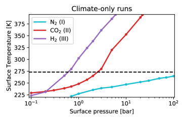
Figure 1: Surface temperature in Kelvin against surface pressure in bar for simulated climate-only N₂-, CO₂-, and H₂-dominated atmospheres of LHS 1140 b (see Table 2). Horizontal dashed line indicates 273 K.

3.2 Atmospheric profiles

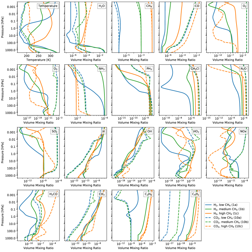
Figure 2: Simulated temperature and composition profiles of selected species of LHS 1140 b. Different colors represent the three types of scenarios considered: blue for low CH₄, green for medium CH₄ and orange for high CH₄. Solid lines represent H₂-dominated atmospheres (scenarios 1a, 1b, and 1c) whereas dashed lines show CO₂-dominated atmospheres (scenarios 10a, 10b, 10c).

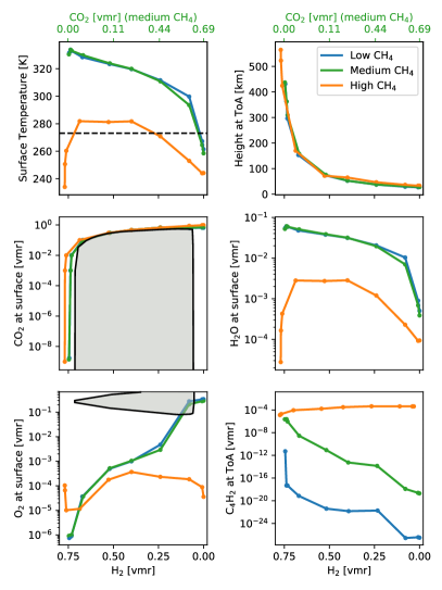
Figure 3: Change in the surface temperature in K, the atmospheric height at ToA ($\sim$0.01 Pa) in km and the surface volume mixing ratio (vmr) of H₂O, O₂, CO and CH₄ with decreasing concentrations of H₂ for scenarios with low (blue lines), medium (green lines) and high CH₄ scenarios. Note that the concentrations of CO₂ corresponding to H₂ vmrs of 0.75, 0.5, 0.25 and 0.0 are shown in green x-labels for the medium CH₄ scenarios. The colored dots represent the 10 individual main scenarios described in Table 3. The dashed black line shows T=273 K. The gray shaded region represents the limits of combustion for H₂-CO₂ and H₂-O₂ gas mixtures (see Grenfell et al., 2018). Note that the assumed surface mixing ratios of H₂ and CO₂ for the main scenarios 5–8 are at the edge of the H₂-CO₂ combustion limit.

To simulate the atmospheric scenarios as described in Section 2.4 we use the coupled version of 1D-TERRA. Figure 2 shows the temperature and composition profiles of selected species for H₂-dominated atmospheres with low concentrations of CO₂ (scenarios 1a, 1b, and 1c; see Sect. 2.4 and Table 3) and CO₂-dominated atmospheres with low concentrations of H₂ (scenarios 10a, 10b, and 10c). Figure 3 shows the surface temperature, the atmospheric height at the Top of Atmosphere (ToA) at $\sim$0.01 Pa, the surface vmr of CO₂, H₂O, and O₂, and the CH₄ vmr at the ToA with decreasing concentrations of H₂ (corresponding to increasing concentrations of CO₂, see Table 3).

3.2.1 Temperature

Figure 2 suggests that the H₂-dominated atmospheres with low and medium CH₄ concentrations (corresponding to scenarios 1a and 1b respectively) show a similar temperature profile from the surface up to $\sim$200 hPa with a strong warming towards the ToA.

The H₂-dominated atmosphere with a high CH₄ concentration (scenario 1c) results in a warm stratosphere due to CH₄ short-wave absorption and accordingly a cool troposphere, similar to the shape of the temperature profile behaviour on e.g. Titan (see e.g. Fulchignoni et al., 2005; Serigano et al., 2016). The large concentration of CH₄ absorbs most of the stellar energy in the stratosphere, leading to reduced stellar irradiation reaching the troposphere (see also Ramirez & Kaltenegger, 2018). Note that 1D-TERRA does not consider the effect of hazes, which might be formed in such an environment (see e.g. He et al., 2018; Hörst et al., 2018).

In CO₂-dominated atmospheres we simulate similar temperature profiles for low CH₄ concentrations (scenario 10a) compared to medium CH₄ concentrations (scenario 10b). There is no temperature inversion from O₃ absorption in the middle atmosphere due to the weak UV emission of M dwarfs (see also e.g. Segura et al., 2005; Grenfell et al., 2014; Wunderlich et al., 2019, 2020). The CO₂-dominated atmosphere with high abundances of CH₄ (scenario 10c) shows weak temperature variations in the range of $\sim$40 K through the simulated atmospheric profile. The high concentration of CH₄ leads to a warming of the atmosphere compared to the runs with lower CH₄ abundances, except near the surface, where the anti-greenhouse effect cools the atmosphere.

In Fig 3 the low and medium CH₄ scenarios (blue and green lines, respectively) feature similar responses in surface temperatures with decreasing H₂. The high CH₄ scenarios (orange line) first show a warming effect of about 50 K due to the decreased partial pressure of CH₄ on increasing the molecular weight towards CO₂-rich atmospheres (scenarios 1c to 4c). Note that the surface mixing ratio of CH₄ is kept constant at 3% for all the high CH₄ scenarios. For CO₂-dominated atmospheres the surface temperature decreases when reducing the abundances of H₂ (scenarios 6c to 10c) due to the weaker warming from the H₂-H₂ CIA.

3.2.2 H₂O

The water profile in the lower atmosphere depends mainly on the assumed relative humidity and the temperature profile near the surface. For all simulations we assume the relative humidity to be constant at 80% up to the tropopause. In the middle and upper atmosphere the H₂O profile is determined mainly by chemical production or loss and to a lesser extent by eddy mixing. H₂O is mainly destroyed by photolysis at wavelengths below 200 nm forming the hydroxyl radical (OH) and atomic hydrogen (H):

$$\text{H${}_{2}$O + h}\nu \rightarrow\text{H + OH.}$$ (R1)

The H₂-dominated atmospheres show weaker FUV absorption compared to the CO₂-dominated atmospheres. This weaker shielding effect leads to enhanced photolysis and less stratospheric water content for the scenarios with H₂-dominated atmospheres (Fig. 2). For the high CH₄ scenarios the water photolysis is weak due to strong FUV absorption from CH₄. In CO₂-dominated atmospheres H₂O is significantly reformed via HO_x-driven (HO_x = H + OH + HO₂) oxidation of CH₄ at pressures less than 0.1 hPa (see also Segura et al., 2005; Grenfell et al., 2013; Rugheimer et al., 2015; Wunderlich et al., 2019).

3.2.3 O₂

All runs assume an Earth-like surface O₂ flux from photosynthesis (see Table 4). However, in H₂-dominated atmospheres the oxygen content near the surface is only $\sim$1 ppm for low and medium CH₄ scenarios (blue and green solid line in Fig. 2). Grenfell et al. (2018) suggest that the catalytic cycles including HO_x and NO_x leads to oxidation of H₂ into water. O₂ is mainly destroyed via photolysis or the three body reaction with atomic hydrogen:

$$\text{O${}_{2}$ + h}\nu \rightarrow\text{O + O}$$ (R2)

$$\text{H + O}_{2}\text{+ M} \rightarrow\text{HO${}_{2}$ + M}$$ (R3)

The atomic hydrogen required for reaction (R3) is mainly produced via:

$$\text{OH + H}_{2} \rightarrow\text{H${}_{2}$O + H.}$$ (R4)

OH can be formed via the reactions:

$$\text{H + HO}_{2} \rightarrow\text{OH + OH}$$ (R5)

$$\text{H + NO}_{2} \rightarrow\text{OH + NO}$$ (R6)

HO₂ + NO $$\rightarrow\text{OH + NO}_{2},$$ (R7)

and by water photolysis (reaction R1) which increases the concentration of H in the middle atmosphere. The atomic hydrogen can be removed via escape or recombines to form H₂ (see Hu et al., 2012). For the H₂-dominated atmosphere with high CH₄ concentrations (scenario 1c) the surface mixing ratio of O₂ is two orders of magnitudes larger than for scenarios 1a and 1b due to the lower concentrations of NO_x and H in the lower atmosphere.

For increasing mixing ratios of CO₂ the destruction of O₂ via H₂ oxidation is less dominant and O₂ can accumulate in the atmosphere (see Fig. 3). The CO₂-dominated atmospheres with less than 10% H₂ feature large abundances of O₂ of up to 30% for the atmospheres with low and medium CH₄ concentrations (scenario 8a–10a and 8b–10b). For the scenarios 8a and 8b the concentration of O₂ might be limited to about 10% (see gray shaded region in Fig 3) due to the potential combustion of the atmosphere (Grenfell et al., 2018).

The large concentrations of O₂ are related to the lower UV flux of M dwarfs (hence weaker O₂ photolysis) as well as strong abiotic production of O₂ from CO₂ photolysis at wavelengths below 200 nm (see also e.g. Domagal-Goldman et al., 2014; Harman et al., 2015; Wunderlich et al., 2020). The lower FUV/NUV ratio of LHS 1140 compared to a solar type star favors the production of abiotic O₂ in CO₂-rich atmospheres via:

$$\text{2(CO${}_{2}$ + h}\nu \rightarrow\text{CO + O)}$$ (R8)

O + O + M $$\rightarrow\text{O}_{2}\text{+ M}$$ (R9)

$$\text{2CO}_{2} \rightarrow\text{2CO + O}_{2}$$

(see also e.g. Selsis et al., 2002; Segura et al., 2007; Tian et al., 2014; France et al., 2016; Wunderlich et al., 2020). The production of O₂ is further enhanced by the presence of OH via:

O + OH $$\rightarrow\text{O}_{2}\text{+ H.}$$ (R10)

CO and O can recombine to CO₂ via a HO_x catalysed reaction sequence, forming CO₂: CO + O $\xrightarrow[]{\text{HO${}_{x}$}}$ CO₂ (see e.g. Domagal-Goldman et al., 2014; Gao et al., 2015; Meadows, 2017; Schwieterman et al., 2019). For the CO₂-dominated atmosphere with high CH₄ concentrations we find that atomic oxygen (O) quickly reacts with CH₃ via:

$$\text{O + CH}_{3} \rightarrow\text{H${}_{2}$CO + H}$$ (R11)

or

$$\text{O + CH}_{3} \rightarrow\text{CO + H${}_{2}$ + H,}$$ (R12)

forming H₂, H, CO and H₂CO. Part of the H₂CO separates into H₂ and CO via:

H₂CO + h$$\nu \rightarrow\text{H${}_{2}$ + CO}$$ (R13)

or

H₂CO + H $$\rightarrow\text{H${}_{2}$ + HCO}$$ (R14)

HCO + H $$\rightarrow\text{H${}_{2}$ + CO.}$$ (R15)

Hence, results suggest low concentrations of O₂ and large abundances of CO for the high CH₄ scenarios with CO₂-dominated atmospheres.

3.2.4 O₃

A main source of O₃ largely depends on the amount of O₂ available for photolysis in the atmosphere. O₂ is split into atomic oxygen via photolysis between 170 and 240 nm (reaction R2) and then reacts with O₂ to form O₃ via a fast three-body reaction (see e.g. Brasseur & Solomon, 2006). The main O₃ sinks are photolysis at wavelengths less than $\sim$200 nm and catalytic cycles involving HO_x and NO_x which convert O₃ into O₂ in the middle atmosphere (see e.g. Brasseur & Solomon, 2006; Grenfell et al., 2013).

In our scenarios, the low FUV/NUV environment compared with the Earth favors weak release of HO_x and NO_x from their reservoir molecules which leads to weak O₃ catalytic loss. The low and medium CH₄ scenarios with CO₂-dominated atmospheres show an ozone layer with peak abundances ($\sim$20–50 ppm) up to about five times larger than on Earth (compare to e.g. Fig. 2 of Wunderlich et al., 2020). Grenfell et al. (2014) suggested that the smog mechanism is an important O₃ source for late M dwarfs since UV levels are not sufficient to drive efficiently the Chapman mechanism. All scenarios with H₂-dominated atmospheres and CO₂-dominated atmosphere with high concentrations of CH₄ are however low in O₂, leading overall to weak production of O₃.

3.2.5 CO

All simulations assume emissions of CO from volcanoes and biomass based on pre-industrial Earth values. An important in-situ sink for CO is OH via:

CO + OH $$\rightarrow\text{CO${}_{2}$ + H}.$$ (R16)

Our results suggest a decreased OH due to a slowing in its main source reaction:

O¹D + H₂O $$\rightarrow\text{2OH},$$ (R17)

since production of O¹D (e.g. from O₃ photolysis) is disfavored by the stellar UV emission. The weak OH favors an increase in CO and CH₄ by several orders of magnitude compared with modern Earth. Similar effects have been noted by several studies in the literature for Earth-like planets (see e.g. Segura et al., 2005; Grenfell et al., 2007; Rugheimer et al., 2015; Wunderlich et al., 2019).

The tropospheric temperature of the H₂-dominated atmosphere with high concentrations of CH₄ (scenario 1c) is much lower compared to the other scenarios due to the strong CH₄ anti-greenhouse effect (see above), leading to water condensation hence less water photolysis in the troposphere. Note that the OH radical can also be formed via HO_x re-partitioning (reaction R7), which can be driven by enhancements in NO e.g. via incoming cosmic rays (see e.g. Airapetian et al., 2016; Scheucher et al., 2018; Airapetian et al., 2020).

In the atmosphere with high concentrations of CH₄ results suggest that the recombination of CO and O into CO₂ is weakened due to the additional sinks of atomic oxygen via reactions (R11) and (R12) as discussed in Section 3.2.3. High CH₄ generally favors lowered OH, which weakens the HO_x catalyzed combination of CO and O into CO₂. This leads to larger abundances of CO for high CH₄ scenarios compared to the other scenarios.

3.2.6 CH₄ and hydrocarbons

Understanding how CH₄ forms higher hydrocarbons (C_n) and how these species are subsequently removed to reform CH₄ is a central issue because higher hydrocarbons can readily condense to form hazes, which could strongly impact climate and observed spectra. The high CH₄ scenarios feature a large production of hydrocarbons such as C₂H₂, C₂H₄ and C₂H₆. Figure 2 shows the atmospheric profiles of C₂H₆ but note that C₂H₂ and C₂H₄ (not shown) have similar concentrations with largest mixing ratios at the ToA with up to 0.1%.

Our results suggest that in H₂-dominated atmospheres the main pathway for initiating ascent of the homologous chain from C₁ $\rightarrow$ C₂ (CH₄ $\rightarrow$ C₂H₆) pathway is as follows:

$$\text{2(CH${}_{4}$ + h}\nu \rightarrow\text{${}^{1}$CH${}_{2}$ + H}_{2})$$ (R18)

$$\text{2(${}^{1}$CH${}_{2}$ + H}_{2} \rightarrow\text{CH${}_{3}$ + H})$$ (R19)

CH₃ + CH₃ + M $$\rightarrow\text{C${}_{2}$H${}_{6}$ + M}$$ (R20)

2CH₄ $$\rightarrow\text{C${}_{2}$H${}_{6}$ + 2H}.$$

The above pathway is an established route for ascending the hydrocarbon chain (see e.g. Yung & DeMore, 1999, Chapter 5 and references therein). It is initiated by CH₄ photolysis to form reactive methyl radicals (CH₃), which participate in a three-body self-reaction to form ethane (C₂H₆).

Our results suggest that C₂H₄ is mainly formed by the reactions:

$$\text{CH + CH}_{4} \rightarrow\text{C${}_{2}$H${}_{4}$ + H}$$ (R21)

and

$$\text{CH${}_{2}$ + CH}_{3} \rightarrow\text{C${}_{2}$H${}_{4}$ + H}$$ (R22)

where CH is produced via:

$$\text{CH${}_{4}$ + h}\nu \rightarrow\text{CH + H${}_{2}$ + H}$$ (R23)

$$\text{CH${}_{3}$ + h}\nu \rightarrow\text{CH + H}_{2}$$ (R24)

or

$$\text{H + CH}_{2} \rightarrow\text{CH + H}_{2}$$ (R25)

and C₂H₂ is formed via photolysis of C₂H₄ and the reaction:

$$\text{CH${}_{2}$ + CH}_{2} \rightarrow\text{C${}_{2}$H${}_{2}$ + H${}_{2}$}$$ (R26)

(see also Yung & DeMore, 1999, and references therein).

In CO₂-dominated atmospheres our results suggest that the reaction (R19) is slower due to reduced H₂ and since part of the CH₂ reacts with CO₂ forming H₂CO and CO. This effect disfavours the pathway producing C₂H₆. Additionally however, the destruction of CH₃ via:

$$\text{CH${}_{3}$ + H}_{2} \rightarrow\text{CH${}_{4}$ + H}$$ (R27)

is weakened due to lowered H₂. This effect favors enhanced CH₃ hence, the pathway producing C₂H₆. The overall effect is slightly lower concentrations of CH₄ in the upper atmosphere but larger amounts of C₂H₆ as well as C₂H₂ and C₂H₄ (not shown) for CO₂-dominated atmospheres compared to H₂-dominated atmospheres when assuming high concentrations of CH₄.

The larger abundances of C₄H₂ shown in Figs. 2 and 3 for the scenario 10c compared to the scenario 1c suggests more haze production by hydrocarbons in CO₂-dominated compared with H₂-dominated atmospheres. Such an effect would be reinforced assuming CO₂-dominated atmospheres have cooler mid to upper atmospheres compared with H₂-dominated atmospheres as suggested by Fig. 2. Note however, that the above result could be reversed in atmospheres where CH₂ (reaction R19) becomes more important for C₂H₆ production since H₂-dominated atmospheres favor reduced CH₂ as discussed above. For the low and medium CH₄ scenarios the concentrations of C₄H₂ decrease with decreasing CH₄/CO₂ ratios as suggested by e.g. Arney et al. (2018) for N₂-dominated atmospheres.

3.2.7 SO₂

We assume volcanic outgassing of SO₂ as measured on modern Earth. Due to its high solubility in water forming sulfate, SO₂ is deposited easily over wet surfaces leading to SO₂ surface mixing ratios below 1 ppb. The main in-situ chemical sink of SO₂ is photodissociation below 400 nm (e.g. Manatt & Lane, 1993) and its oxidation via reaction with OH or O₃ to form ultimately SO₃ which quickly reacts with water to form sulfate (see e.g. Burkholder et al., 2015; Seinfeld & Pandis, 2016). In CO₂-dominated atmospheres with low and medium CH₄ concentrations (scenarios 10a and 10b), results suggest that shielding associated with large UV absorption from CO₂, O₂, and O₃, enables the concentrations of SO₂ to reach up to 1 ppm in the stratosphere.

In H₂-dominated atmospheres the high UV environment leads to low abundances of SO₂ over the entire atmosphere. Note that strong SO₂ abundances in e.g. moist, warm tropospheres (see Figure 2) would favor significant sulfate aerosol formation although a strong hydrological cycle would quickly wash out the sulfate formed (see e.g. Loftus et al., 2019).

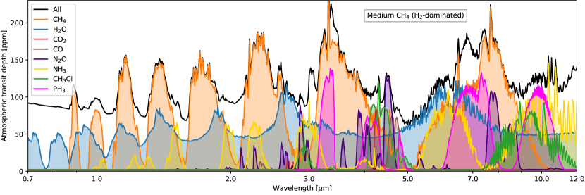
Figure 4: Simulated transmission spectrum of the medium CH₄ scenario with the H₂-dominated atmosphere (scenario 1b) binned to a constant resolving power of $R$=300 (maximum resolving power of JWST NIRSpec PRISM at 5 $\mu$m). The black line represents the spectrum which includes the contribution from all gases which are considered in 1D-TERRA and also available in HITRAN, Rayleigh scattering, aerosol extinction, H₂O CKD and CIAs. Individual gaseous absorption of selected molecules are represented by different colors.

3.2.8 Potential biosignatures NH₃, PH₃, CH₃Cl and N₂O

The chemical destruction of NH₃, PH₃, and CH₃Cl is controlled by reactions with OH, O¹D, H and by photodissociation in the UV (see e.g. Segura et al., 2005; Seager et al., 2013b; Sousa-Silva et al., 2020). In the middle atmosphere NH₃ photodissociates into NH₂ and H. In H₂-dominated atmospheres the NH₂ reacts quickly with H and reforms NH₃. In the high CH₄ atmosphere this recombination process is slower due to enhanced HO₂ from water photolysis in the stratosphere leading to more destruction of atomic hydrogen by reaction (R5) (see also Sec. 3.2.3). Our results suggest that an assumed emission of 8.38$\times$10¹⁰ molecules cm^-2 s^-1 would lead to NH₃ surface mixing ratios between 0.1 and 1 ppm. This is consistent with the results from Seager et al. (2013b) who obtain an NH₃ mixing ratio of 0.1 ppm with surface flux of 5.1$\times$10¹⁰ molecules cm^-2 s^-1 for a planet with an H₂-dominated atmosphere around an active M dwarf.

For PH₃ we assume an emissions flux of 1$\times$10¹⁰ molecules cm^-2 s^-1 and obtain a surface mixing ratio of about 200 ppb for the H₂-dominated atmosphere with low CH₄ concentrations. Sousa-Silva et al. (2020) find similar mixing ratios of PH₃ when assuming a ten times larger surface flux for a planet with an H₂-dominated atmosphere around an active M dwarf. However, they did not consider that PH₃ may be recycled via chemical reactions with H or H₂.

For CO₂-dominated atmospheres with low and medium concentrations of CH₄ (scenarios 10a, 10b) the destruction of PH₃ from H is weaker compared to H₂-dominated atmospheres and we obtain larger surface mixing ratios of several ppm. Given the weak recycling of PH₃ from H or H₂, our results are consistent with Sousa-Silva et al. (2020) who obtain a mixing ratio of 15 ppm for a ten times larger surface flux. For the high CH₄ scenario (10c) our results suggest that large abundances of OH are produced near the surface via:

$$\text{CH${}_{3}$ + O}_{2} \rightarrow\text{H${}_{2}$CO + OH},$$ (R28)

leading to enhanced destruction of PH₃ compared to the other scenarios. The CH₃Cl and N₂O loss processes are dominated by photolysis in the UV below 240 nm and reaction with O¹D (see also e.g. Grenfell et al., 2013). Due to the low UV environment in CO₂-dominated atmospheres, the destruction by photolysis is weaker and the abundances of CH₃Cl and N₂O are larger compared to the H₂-dominated atmospheres.

3.2.9 Atmospheric height

The right upper panel of Fig. 3 shows atmospheric height at the ToA for all simulated scenarios. A central aim of this paper is to investigate whether it is feasible to detect atmospheric molecular features on LHS 1140 b with future telescopes. A large atmospheric height leads to stronger absorption features in transmission spectroscopy and hence to improved detectability of the corresponding species. Due to the low mean molecular weight hence larger scale height of the H₂-dominated atmospheres, the ToA at $\sim$0.01 Pa occurs at a height of up to 570 km, whereas the CO₂-dominated atmospheres only reach an altitude of about 35 km. The larger stratospheric temperatures for the high CH₄ scenarios furthermore lead to an expansion of the atmosphere compared to the scenarios with less CH₄.

3.3 Transmission spectra

Table 6: Central wavelength, $\lambda_{\text{c}}$ ($\mu$m), of molecular bands from NH₃, PH₃, CH₃Cl, and N₂O and spectral features which might overlap or obscure the bands at the corresponding $\lambda_{\text{c}}$.

Species	$\lambda_{\text{c}}$	Overlap
N2O	2.9 $\mu$m	CO2
N2O	4.5 $\mu$m	CO, CO2
NH3	2.0 $\mu$m	H2O, H2-H2, haze, CO2
NH3	3.0 $\mu$m	CO2, C2H2
NH3	6.1 $\mu$m	CH4, H2O
NH3	10.5 $\mu$m	H2-H2, O3, CO2
PH3	4.3 $\mu$m	CO2
PH3	9.5 $\mu$m	H2-H2, O3, CO2
CH3Cl	3.3 $\mu$m	CH4
CH3Cl	7.0 $\mu$m	CH4, H2O, C2H6
CH3Cl	9.8 $\mu$m	H2-H2, O3, CO2

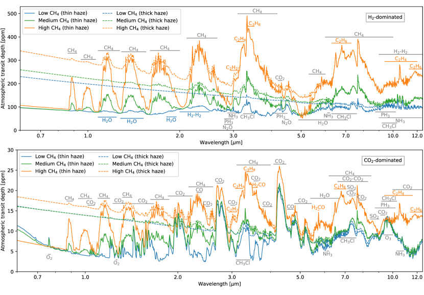
Figure 5: Simulated atmospheric features of the LHS 1140 b for all three scenarios with H₂- (upper panel) and CO₂-dominated atmospheres (lower panel), represented by cloud-free transit transmission spectra and binned to a constant resolving power of $R$=300. The scenarios are indicated by the different colors: blue for low concentrations of CH₄ (scenario 1a for H₂- and scenario 10a for CO₂-dominated atmospheres), green for medium concentrations of CH₄ (scenario 1b for H₂- and scenario 10b for CO₂-dominated atmospheres) and orange for high concentrations of CH₄ (scenario 1c for H₂- and scenario 10c for CO₂-dominated atmospheres). Important atmospheric molecular absorption are highlighted with horizontal lines in the color of the scenario with a strong absorption feature or in gray when all scenarios show a strong feature. Solid lines include weak extinction from hazes whereas dashed lines consider extinction by thick hazes.

Figure 4 shows the simulated transmission spectrum of LHS 1140 b for the H₂-dominated atmosphere with medium CH₄ concentrations (scenario 1b). The contribution from individual molecular absorption bands is shown with different colors. To detect a spectral band with e.g. the JWST it is important to identify a wavelength range which is not obscured by the absorption of other molecules or haze extinction. The strongest spectral features are due to absorption by CH₄. Below $\sim$2 $\mu$m molecular features of H₂O and NH₃ are obscured by haze extinction, which increases the transit depth to $\sim$90 ppm. Between 2 and 2.5 $\mu$m H₂-H₂ CIA contributes significantly to the transmission spectrum (see Abel et al., 2011).

Around 3.0 $\mu$m we obtain two absorption features mainly produced by NH₃, N₂O and PH₃. Absorption by CH₄ and H₂O is rather weak at these wavelengths. However, between 3.0 and 3.1 $\mu$m C₂H₂ contributes significantly to the spectral feature (not shown). The absorption by CO₂ around 3.0 $\mu$m is significant for atmospheres with mixing ratios of $\sim$1% or more CO₂ (not shown). The spectral features of CH₃Cl around 3.3 $\mu$m and 7 $\mu$m overlap with absorption by CH₄ and H₂O. For CO₂-poor atmospheres the features from N₂O and PH₃ dominate the spectrum between 4.1 and 4.6 $\mu$m. However, Earth-like CO₂ levels lead to a strong absorption feature around 4.3 $\mu$m (see e.g. Rauer et al., 2011; Wunderlich et al., 2019).

Between 9 and 12 $\mu$m we find strong absorption by PH₃, NH₃ and CH₃Cl. For H₂-dominated atmospheres there is a significant contribution from H₂-H₂ CIA (not shown) to the transmission spectrum (Abel et al., 2011; Fletcher et al., 2018). In CO₂ atmospheres these features might overlap with absorption by O₃ and CO₂. Many of the simulated atmospheric spectral features of N₂O, NH₃, PH₃ or CH₃Cl overlap with other molecular bands of e.g. CO₂ or CH₄ (see Table 6). However, at some spectral bands these potential biosignatures contribute significantly to the full feature offering the possibility to detect the additional absorption if the abundances of CO₂ and CH₄ are known. Figure 5 shows the simulated transmission spectra of H₂-dominated atmospheres (scenarios 1a, 1b, and 1c) and CO₂-dominated atmospheres (scenarios 10a, 10b, and 10c). We take into account the effect of weak extinction from thin hazes (solid line) and from thick Titan-like hazes (dashed line).

For the high CH₄ scenarios the mean transit depth is increased compared to the other two scenarios due to strong absorption by CH₄ and the warm stratospheric temperature which leads to an expansion of the atmosphere. Due to the low molecular weight of the H₂-dominated atmospheres the spectral features are generally larger than in CO₂-dominated atmospheres. The extinction by thick haze significantly increases the transit depth at atmospheric windows up to 6 $\mu$m. Hazes at large altitudes are considered to be the main reason for the observed flat spectrum of e.g. GJ 1214 b (Bean et al., 2010; Désert et al., 2011; Kempton et al., 2011; Kreidberg et al., 2014). However, HST observations of the atmosphere of LHS 1140 b suggest a clear atmosphere (Edwards et al., 2020). In the following text we compare the observed spectrum with our simulations.

3.4 Comparison to observations

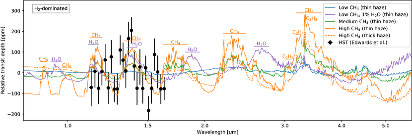
Figure 6: Simulated spectral features compared to HST observations taken from Edwards et al. (2020), assuming H₂-dominated atmospheres. The scenarios are indicated by the different colors: solid blue line for the low CH₄ scenario (1a) as shown in Fig. 5 and the solid purple line for scenario 1a but with an assumed constant H₂O mixing ratio of 1%; solid green line for the medium CH₄ scenario (1b); solid and dashed orange lines for the high CH₄ scenario (1c) with thin and thick hazes, respectively. All spectral data were binned to $R$=300 and subtracted from the mean transit depth between 1.1 and 1.7 $\mu$m.

Diamond-Lowe et al. (2020) combined two spectrally resolved transit observations of LHS 1140 b from the optical to the NIR (610–1010 nm). Their median uncertainty of the transit depth was 260 ppm. They concluded that about a factor of 4 higher precision would be needed to detect a clear hydrogen-dominated atmosphere. The strongest spectral feature of CH₄ at $\sim$900 nm has a strength of about 130 ppm assuming weak extinction by hazes (solid orange line in Fig. 5). The slope from extinction by thick hazes between 610 and 1010 nm leads to a decrease of the transit depth by $\sim$50 ppm (dashed orange line in Fig. 5, upper panel). Hence, our results confirm that the precision of transit observations between 610 and 1010 nm shown by Diamond-Lowe et al. (2020) is not large enough to draw a conclusion on the atmosphere of LHS 1140 b.

Recently, Edwards et al. (2020) presented HST transit observations between 1.1 and 1.7 $\mu$m. They concluded that a maximum in the spectrum around 1.4 $\mu$m might suggest an evidence of water vapour absorption in a clear H₂/He atmosphere. However, due to the large stellar contamination and the low overall signal-to-noise ratio further observation time is required to confirm the detection of a planetary atmospheric feature. Figure 6 compares the spectrally resolved HST observations with simulated spectra assuming H₂-dominated atmospheres (scenarios 1a, 1b, and 1c). The low CH₄ scenario shows a mixing ratio of H₂O below 1 ppm in the middle atmosphere (see Fig. 2) and the resulting spectrum shows only a weak feature at 1.4 $\mu$m (blue line). In Edwards et al. (2020) the water vapour abundance has been retrieved to log₁₀(V${}_{\text{H${}_{2}$O}}$) = -2.94${}^{+1.45}_{-1.49}$. When assuming a H₂O mixing ratio of 1%, constant over height, we find a difference in the transit depth of about 150 ppm between 1.4 $\mu$m and 1.6 $\mu$m. However, such large abundances of H₂O are not consistent with the results of our photochemical model simulations for thin H₂-dominated atmospheres with habitable surface temperatures. Large abundances of H₂O in thick H₂-atmospheres, which were not considered here, might be consistent with our model but would lead to surface temperatures above 395 K (see Fig. 1), which are unlikely to sustain life (see e.g. Bains et al., 2015).

Figure 6 suggests that a large spectral feature of $\sim$200 ppm at 1.4 $\mu$m can be also obtained by strong CH₄ absorption in a thin H₂-dominated atmosphere containing several percent of CH₄ and limited haze production. Large abundances of CH₄ might favor the formation of hydrocarbon haze (He et al., 2018; Hörst et al., 2018; Lavvas et al., 2019). However, Fig. 2 suggests that the haze production is lower compared to CO₂-dominated atmospheres with high CH₄ abundances (see Section 3.2.6).

Similarly to our finding regarding the atmosphere of LHS 1140 b, the model studies by Bézard et al. (2020) and Blain et al. (2020) suggest that the detected spectral feature at 1.4 $\mu$m in the atmosphere of K2-18 b (Benneke et al., 2019; Tsiaras et al., 2019) might be produced by CH₄ rather than H₂O. They concluded that the H₂O-dominated spectrum interpretation is either due to the omission of CH₄ absorption or a strong overfitting of the data. Further observations with e.g. the Very Large Telescope (VLT) or the JWST are expected to confirm or rule-out the existence of large abundances of CH₄ in the atmosphere of LHS 1140 b or K2-18b (see e.g. Edwards et al., 2020; Blain et al., 2020). In the following we further determine the capabilities of the upcoming generation of telescopes with increased sensitivity and larger wavelength coverage to characterize the atmosphere of LHS 1140 b.

3.5 Detectability of spectral features with JWST and ELT

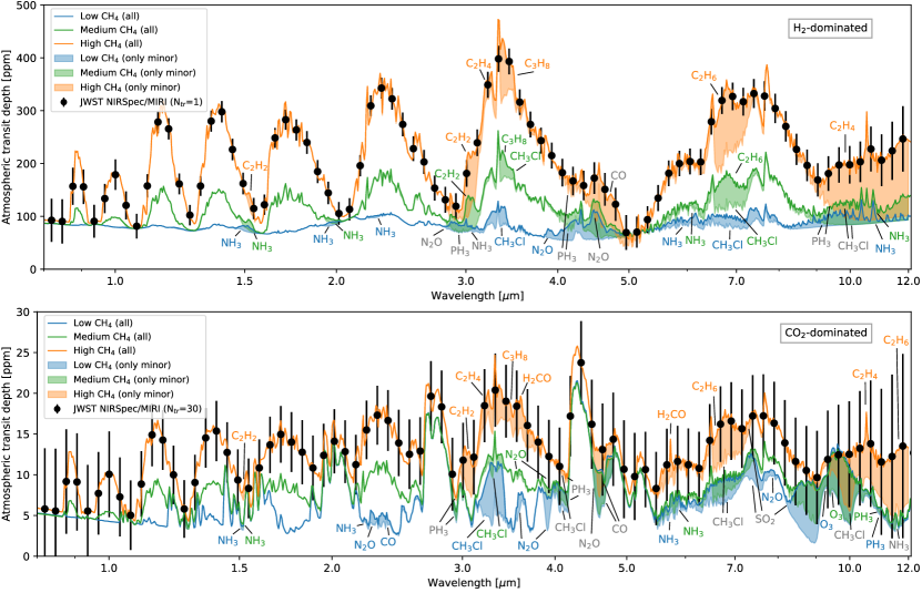
Figure 7: Simulated transmission spectra of LHS 1140 b with weak extinction from hazes in solid lines as shown in Fig. 5. The upper panel shows H₂-dominated atmospheres with low, medium and high CH₄ concentrations corresponding to scenarios 1a (blue), 1b (green), and 1c (orange), respectively. The lower panel shows CO₂-dominated atmospheres with low, medium and high CH₄ concentrations corresponding to scenarios 10a (blue), 10b (green), and 10c (orange), respectively. The shaded region shows the contribution of the minor species to the full spectrum. Expected error bars for a single transit observation assuming scenario 1c (upper panel) and 30 co-added transits assuming scenario 10c (lower panel) using JWST NIRSpec PRISM (0.7–5 $\mu$m) and JWST MIRI LRS (5–12 $\mu$m), binned to $R$=30. Strongest contribution of minor atmospheric molecular absorption bands are indicated by the color of the scenario or in gray when all scenarios have a significant contribution.

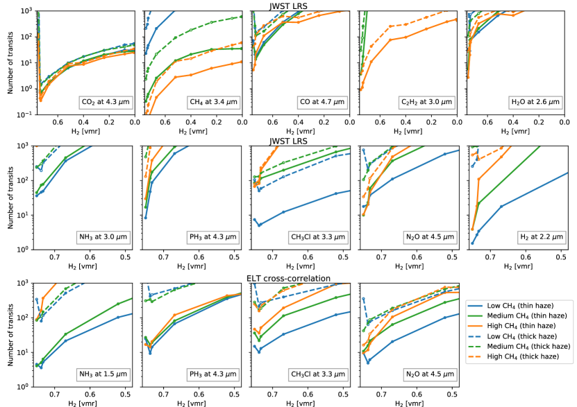
Figure 8: Number of transits required to reach an S/N of 5 for the corresponding spectral features in a cloud free atmosphere with thin (solid lines) and thick (dashed lines) hazes using low resolution transmission spectroscopy with JWST NIRSpec PRISM (upper and middle panels) and the cross-correlation technique with high resolution transmission spectroscopy using ELT HIRES or METIS (lower panels). Note that the x-axis of the upper panel is different to the middle and lower panel. Each colored circle corresponds to one scenario from Table 3. Blue lines and circles show low CH₄ scenarios, green lines and circles show medium CH₄ scenarios and orange lines and circles show high CH₄ scenarios.

To determine the number of transits which are required to detect a spectral feature (S/N = 5) we subtract the full transmission spectra (including the absorption from all species, CIAs, H₂O CKD, Rayleigh extinction and extinction from hazes) from the spectrum excluding the contribution from the corresponding species. Thus, we consider only the contribution of these species to the full spectrum. This method assumes that we know the concentration of other main absorber such as CH₄ or CO₂, which may overlap with the spectral bands (see Table 6). Note that other molecules could mimic large scale features of the molecule in question. Hence, retrieval analysis (see Barstow & Heng, 2020, for a recent overview) or the detection of the molecules at multiple wavelengths would be required to exclude an ambiguity.

Second, for LRS with JWST NIRSpec we bin the spectral data until the optimal value is found, leading to the lowest required number of transits. Binning the data decreases on the one hand the noise contamination but on the other hand, large wavelength ranges can lead to interfering overlaps of absorption bands and atmospheric windows. Due to the unknown systematic error when binning the synthetic spectral data we assume only white noise for the binning. This gives an optimistic estimation on the detection feasibility of the JWST. Note that we do not consider the wavelength range between 1 and 2 $\mu$m due to the saturation of the detector for NIRSpec PRISM. However, due to extinction by hazes the detection of the spectral features of e.g. CH₄ and CO₂ at this wavelength range would require similar or more observation time than the features at longer wavelengths. For the high resolution spectra we use a constant resolving power of $R$=100,000 as planned for the HIRES and METIS on ELT and apply the cross-correlation technique with the same method as presented in Wunderlich et al. (2020). We do not show results from emission spectroscopy in this study due to the much larger required observation time compared to transmission spectroscopy for planets in the habitable zone (see e.g. Rauer et al., 2011; Lustig-Yaeger et al., 2019).

At most wavelengths the simulated spectra are dominated by major absorbing species (here defined as H₂, He, CO₂, CH₄, and H₂O). To identify suitable wavelength ranges for the detection of minor absorbers (here defined as all non-major species), the spectrum including only major absorbers was subtracted from the full spectrum. The remainder, representing the contribution of the minor absorbers to the full spectrum, is shown in the shaded region in Fig. 7. The expected error bars of the simulated H₂-dominated atmospheres observed by JWST NIRSpec PRISM or MIRI LRS suggest that a detection of minor absorbers will be challenging within a single transit (upper panel of Fig. 7). However, multiple transits might improve the S/N sufficiently to detect those features.

In CO₂-dominated atmospheres the larger molecular weight decreases the features in the transmission spectra compared to H₂-dominated atmospheres. The error bars in the lower panel of Fig. 7 arise from 30 co-added transit observation with JWST, which would correspond to a period of two years if each transit of LHS 1140 b were to be observed. The results suggest that it will be very challenging to detect minor absorbers in a CO₂-dominated atmosphere during the lifetime of JWST. The detection of major absorbers such as CO₂ or CH₄ might be feasible but also challenging. This is consistent with the results of Morley et al. (2017), who suggest that the detection of a Venus-like atmosphere on LHS 1140 b would require over 60 transits with JWST.

The upper panel of Fig. 8 suggests that CO₂ is detectable at 4.3 $\mu$m for mixing ratios between $1\times 10^{-3}$ and 0.1 within a few transits. For the scenarios 1a, 1b, and 1c with only 1 ppb CO₂ the spectral features are too weak to allow for a detection of CO₂ (see also Fig. 4). The detection of CO₂ is only weakly dependent on the amount of CH₄ in the atmosphere. The high CH₄ cases require less transits due to the larger atmospheric heights from CH₄ heating in the middle atmosphere (see Fig. 3). The detection of CH₄ in a clear H₂-dominated atmosphere requires only one transit observation with CO₂ concentrations of less than 10% for the high CH₄ scenarios and with less than 1% CO₂ for the medium CH₄ scenarios. When assuming thick hazes the detection of CH₄ would require about ten times more transits for the medium and low CH₄ scenarios. For the high CH₄ scenarios the impact of haze extinction on the detectability of CH₄ is weaker. For CO₂-dominated atmosphere the detection of the 3.4 $\mu$m CH₄ feature will be challenging with transmission spectroscopy. The detectability of CH₄ and CO₂ is not significantly improved when applying the cross-correlation technique with observations by ELT HIRES or METIS (not shown, see e.g. Wunderlich et al., 2020).

For each of the atmospheric scenarios we assume a strong dry deposition of CO (see Table 4) leading to weak accumulation of CO from CO₂ photolysis in CO₂-rich atmospheres compared to previous model studies (Schwieterman et al., 2019; Hu et al., 2020; Wunderlich et al., 2020). Hence, the detection of CO will be challenging in the atmospheres we consider. Hydrocarbons such as C₂H₂ are formed in large abundances for the high CH₄ case and could be detectable with less than 10 transits in CO₂ poor, H₂-dominated atmospheres.

The number of transits required to detect H₂O is lowest for the H₂-dominated atmosphere with high CH₄ concentration (scenario 1c). This scenario has the lowest surface water vapor but large amounts of chemically produced H₂O in the stratosphere. Hence, the detection of water in transmission spectroscopy is only weakly related to the presence of liquid surface water in these cases.

In the middle panel of Fig. 8 we show the number of transits required to detect spectral features from NH₃, PH₃, CH₃Cl, N₂O, and the CIA from H₂-H₂ using JWST NIRSpec PRISM. The lower panel of Fig. 8 shows the number of transits required to detect spectral features from NH₃, PH₃, CH₃Cl, and N₂O using ELT HIRES. Note that we show only the scenarios with H₂ mixing ratios of more than 50%. For CO₂-poor atmospheres with low or medium concentrations of CH₄ (scenarios 1a–3a and 1b–3b) the results suggest that the detection of NH₃ would require tens to hundreds of transits with JWST NIRSpec PRISM and the spectral lines of NH₃ around 1.5 $\mu$m might be detectable with about five transits with ELT HIRES. The detection of NH₃ around 2.3 $\mu$m would require around 8 transits (not shown). However, due to possibility of a simultaneous detection of spectral lines from CH₄, H₂O and CO this wavelength region might be favorable for HRS (Brogi & Line, 2019). Strong extinction by hazes or large absorption by CH₄ for the high CH₄ scenarios would prevent the detection of NH₃.

The spectral feature of PH₃ at 4.3 $\mu$m might be detectable within 10–30 transits for the H₂-dominated atmospheres with 1 ppb CO₂ (scenarios 1a, 1b, and 1c) and weak extinction by hazes. For the other scenarios the PH₃ feature is obscured by the CO₂ absorption band around 4.3 $\mu$m (see also Sousa-Silva et al., 2020). The detectability of PH₃ is improved using high resolution spectra of ELT METIS compared to JWST observations for CO₂-rich atmospheres. However, for more than 1% of CO₂ mixing ratios the detection of PH₃ would require tens to hundreds of transits.

For H₂-dominated atmospheres with high concentrations of CH₄ (scenario 1c) the mixing ratios of CH₃Cl are larger compared to scenarios 1a and 1b (see Fig. 2). However, the strongest spectral band of CH₃Cl in the wavelength range of JWST NIRSpec PRISM overlaps with absorption by CH₄ (see Fig. 4), owing to a better detectablility of CH₃Cl in CH₄-poor atmospheres. Similar observation time is required to detect CH₃Cl with JWST and with ELT for the low CH₄ scenarios. However, the cross-correlation technique is less sensitive to the increase in CH₄ compared to LRS. Note that 10 transit observations with JWST would be feasible within one or two years (given a 24.7 days orbital period of LHS 1140 b, Dittmann et al., 2017) but ground-based facilities would require a much longer observation period because less transits could be captured per year. N₂O might be detectable within 10 to 20 transits in CO₂-poor atmospheres with thin hazes. Results suggest weak dependence of the detectability of N₂O on the concentration of CH₄.

Our paper suggests that the detection of potential biosignatures with JWST or ELT is feasible for clear, H₂-dominated atmosphere but would require several transit observations. If such a molecule would be detected, retrieval analysis might challenge to constrain its abundance with low uncertainties due to sparse knowledge on broadening coefficients (see e.g. Tennyson & Yurchenko, 2015; Hedges & Madhusudhan, 2016; Barton et al., 2017; Fortney et al., 2019) and hence, it would be difficult to rule out a potential abiotic origin.

4 Summary and Conclusion

In this study we used a self-consistent model suite to simulate the atmosphere and spectral appearance of LHS 1140 b. First we performed climate only runs to determine the surface pressures for which the Super-Earth LHS 1140 b would have habitable surface conditions in N₂, H₂ and CO₂ atmospheres. Our results suggest that a thick N₂-dominated atmosphere on LHS-1140 b or substantial amounts of greenhouse gases such as CO₂ would be required to reach habitable surface temperatures. A $\sim$2.5 bar CO₂ atmosphere or a $\sim$0.6 bar H₂-He atmosphere would lead a surface temperature of $\sim$273 K. In a second step we used these results and assumed a fixed surface pressure of 2.416 bar (corresponding to the atmospheric mass of the Earth) to simulate potential CO₂- and H₂-dominated atmospheres of LHS 1140 b with our coupled climate-photochemistry model, 1D-TERRA. We simulated possible composition of the planetary atmospheres, assuming fixed biomass emissions and varying boundary conditions for CH₄.

The results suggest that the amount of atmospheric CH₄ can have a large impact upon the temperature and composition of H₂-dominated atmospheres. A few percent of CH₄ may be enough to lower the surface temperatures due to an anti-greenhouse effect. In H₂-dominated atmospheres with high concentrations of CH₄ this effect dominates, leading to a cooling of up to 100 K and the stratosphere is pronounced with temperatures up to 70 K warmer than those at the surface. Although we did not consider the effect of hydrocarbon hazes in the climate-chemistry model, e.g. Arney et al. (2017) have shown that this is expected to warm the surface temperature by only a few degrees. For CO₂ atmospheres the temperature profile is less affected by CH₄ absorption due to CO₂ cooling in the stratosphere.

In H₂-dominated atmospheres O₂ is efficiently destroyed preventing significant concentrations of O₂ and O₃ in such environments. Hence, even if O₂ and O₃ were biosignatures, they would not be detectable in the atmosphere of such a habitable planet which is dominated by H₂. In CO₂-dominated atmospheres O₂ and O₃ can be produced abiotically which might lead to a false-positive detection (see also Selsis et al., 2002; Segura et al., 2007; Harman et al., 2015; Meadows, 2017; Wunderlich et al., 2020). However, results suggest that large amounts of CH₄ would also lead to low concentrations of O₂ and O₃.

We consider NH₃, PH₃, CH₃Cl and N₂O to be potential biosignatures in H₂ and CO₂ atmospheres. Here the main constituent of the atmosphere has a weak impact on the concentrations of these potential biosignatures assuming that the emission flux is the same for both H₂ and CO₂ atmospheres (see also Seager et al., 2013b; Sousa-Silva et al., 2020). However, the detectability of molecules with transmission spectroscopy largely depends on the main composition of the atmosphere due to the difference in mean molecular weight.

First observations of the planet suggest that the atmosphere of LHS 1140 b has a low mean molecular weight (Edwards et al., 2020). In a thin, H₂-dominated atmosphere our results suggest that the tentative spectral feature at 1.4 $\mu$m might be produced by CH₄ rather than H₂O. If the feature at 1.4 $\mu$m were produced by water vapour absorption, surface temperatures are unlikely to be habitable. Our results suggest that the molecular features of CH₄ and CO₂ for habitable surface conditions might be detectable within one transit using JWST NIRSpec observations around 3.4 $\mu$m and 4.3 $\mu$m, respectively. At these wavelengths the absorption cross section of H₂O is weak and at large wavelengths the extinction by hazes has only a weak impact on the detectability of spectral features. The detection of NH₃, PH₃, CH₃Cl or N₂O would require about 10–50 transits ($\sim$40–200 h) with JWST, assuming clear conditions. The molecular bands of these species overlap with absorption by CO₂ or CH₄ in most cases, making a detection more challenging.

With high resolution spectroscopy using ELT HIRES or METIS individual absorption lines are distinguishable which might improve the detectability of potential biosignatures. Our results suggest that NH₃ might be detectable with less than 20 h of ELT observing time in H₂-dominated atmospheres with low or medium CH₄ mixing ratios. A thick haze layer in the atmosphere would, however prevent the detection of any potential biosignature. Strong spectral lines of PH₃, CH₃Cl and N₂O feature in the wavelength range of ELT METIS with overall lower sensitivity compared to ELT HIRES (see e.g. Wunderlich et al., 2020).

Results suggest that a single transit observation of LHS 1140 b with JWST NIRSpec would be enough to confirm or rule out the existence of a clear H₂-dominated atmosphere as suggested by recent observations (Edwards et al., 2020). Such an observation would further help better constrain the atmospheric CH₄. If future observations suggest a thin H₂-dominated atmosphere on LHS 1140 b, the planet is one of the best currently known targets to find potential biosignatures such as NH₃ or CH₃Cl in the atmosphere of an exoplanet in the habitable zone with a reasonable amount of JWST or ELT observation time.

Appendix A Neptune validation

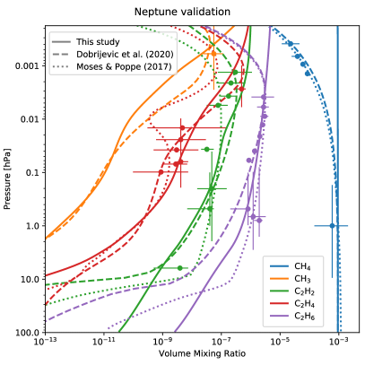
Figure 9: Neptune composition profiles for CH₄ (blue), CH₃ (orange), C₂H₂ (green), C₂H₄ (red) and C₂H₆ (purple) calculated with our photochemistry model indicated with solid lines, compared to the model results of Dobrijevic et al. (2020) with dashed lines, Moses & Poppe (2017) (dotted lines) and a range of multiple observations (dots and corresponding error bars; see text for details).

Figure 9 shows stratospheric composition profiles of selected species in the Neptunian atmosphere, simulated with the photochemistry model BLACKWOLF (Wunderlich et al., 2020). We use the atmospheric temperature profile from Fletcher et al. (2010), inferred from infrared measurements. The profiles are compared to observations and results from Dobrijevic et al. (2020) and Moses & Poppe (2017). The observations are taken from numerous studies as follows: CH₄ from Yelle et al. (1993); Fletcher et al. (2010) and Lellouch et al. (2015); CH₃ from Bezard et al. (1999); C₂H₂, C₂H₄ and C₂H₆ from Yelle et al. (1993); Fletcher et al. (2010) and Greathouse et al. (2011).

The lower boundaries at 100 hPa are set to a constant mole fraction, $f$, for He, CH₄, CO, CO₂ and H₂O respectively to $f_{\text{He}}$ = 0.19 (Williams et al., 2004), $f_{\text{CH}_{4}}$ = 9.3$\times$10^-4 (Lellouch et al., 2015), $f_{\text{CO}}$ = 1.1$\times$10^-6 (Luszcz-Cook & de Pater, 2013), $f_{\text{CO}_{2}}$ = 5 $\times$ 10^-10 (Feuchtgruber et al., 1999). H₂ is set to be the fill gas in each layer to make up the total volume mixing ratio to unity. For all other species we assume a downward flux given by the maximum diffusion velocity, $v=K_{\text{0}}/H_{0}$, where $K_{\text{0}}$ is the eddy diffusion coefficient and $H_{0}$ the atmospheric scale height at the lower boundary. The eddy diffusion coefficient over height, K${}_{\text{{zz}}}$ (in cm²s^-1), are adapted from (Moses et al., 2018):

$$K{{}_{\text{zz}}}=\cases{1}0^{5}\left(\frac{0.1}{P}\right)^{0.55},&\text{if $p\leq$ 0.5 Pa}\\ 10^{4}\left(\frac{0.1}{P}\right)^{0.98},\text{if 0.5 Pa > $p$ > 280 Pa}\\ 400,\text{ if $p\geq$ 280 Pa}{}$$ (2)

Results suggest that the Neptunian atmosphere, as simulated by the photochemistry model, compares well both with the observations as well as with the results from Dobrijevic et al. (2020) and Moses & Poppe (2017). Observations for pressures below 0.1 hPa however suggest a depletion of CH₄, which is not predicted in our model. In the stratosphere of Neptune molecular diffusion is the main process that controls the relative abundance of CH₄ above the methane homopause. The model version applied here includes Eddy diffusion but not molecular diffusion, consistent with an overestimation of the CH₄ concentrations below 0.1 hPa.

Appendix B Titan

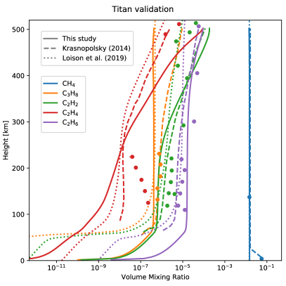
Figure 10: Titan composition profiles for CH₄ (blue), C₃H₈ (orange), C₂H₂ (green), C₂H₄ (red) and C₂H₆ (purple) calculated with our photochemistry model (solid lines), compared to the results from Loison et al. (2019) (dashed lines), Krasnopolsky (2014) (dotted lines) and a range of multiple observations (dots and corresponding error bars; see text for details).

Figure 10 shows the composition profiles of selected species in the atmosphere of Titan, calculated with BLACKWOLF and compared to the results from Loison et al. (2019) and Krasnopolsky (2014). The observations are taken from Nixon et al. (2013); Kutepov et al. (2013) and Koskinen et al. (2011).

At the surface (1.45 bar) we set a constant mole fraction, $f$, for CH₄, CO and H₂ respectively to $f_{\text{CH}_{4}}$ = 0.015 (Niemann et al., 2010), $f_{\text{CO}}$ = 4.7 $\times$ 10^-5 (de Kok et al., 2007) and $f_{\text{H}_{2}}$ = 1 $\times$ 10^-3 (Niemann et al., 2010). N₂ is set to be the fill gas in each layer. For all other species we assume a dry deposition velocity of 0.02 cm/s. The eddy diffusion profile is taken from Krasnopolsky (2014). The temperature profile is taken from Loison et al. (2019).

Our simulated atmosphere of Titan compares reasonably well with the results of Krasnopolsky (2014) and Loison et al. (2019) and is consistent with the observations. Note that we simulate annual and global mean conditions with the model whereas the measurements do not represent the full range of temporal and spatial variations in the atmosphere of Titan. Profiles of latitudinal variations of the atmospheric composition of Titan are shown in Vinatier et al. (e.g. 2010).

Appendix C Representation of thick hazes in GARLIC

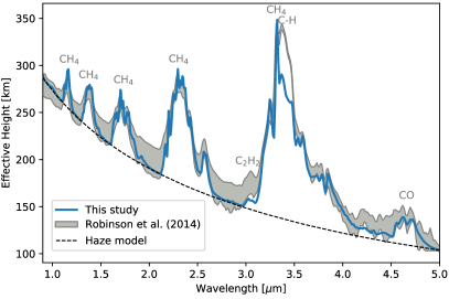
Figure 11: Transit transmission spectrum for Titan represented by effective height in km (blue solid line). The shaded region indicates deviations from four individual transit spectra taken from Robinson et al. (2014). The black dashed line shows the best fit haze model.

We simulate the transmission spectrum of Titan with GARLIC using the output of BLACKWOLF (see Appendix B). Since the ToA for Titan in our model is at $\sim$500 km, we use the data from Loison et al. (2019) to extend the atmosphere up to 1500 km. GARLIC represents the extinction by hazes using Eq. (1). We vary $\alpha$ and $\beta$ to fit the transmission spectrum from Robinson et al. (2014) observed by the Visual and Infrared Mapping Spectrometer (VIMS) from Brown et al. (2004) aboard the Cassini spacecraft. The best fit is presented in Fig. 11 using $\alpha=2.6$ and $\beta=6.0\times 10^{-25}$. We use these values to simulate the impact of extinction from thick hazes in the atmosphere of LHS 1140 b.

The CH₄ absorption features are reproduced well by GARLIC. We underestimate the absorption of the C-H stretching mode of aliphatic hydrocarbon chains near 3.4 $\mu$m (see Bellucci et al., 2009; Maltagliati et al., 2015). This discrepancy is likely due to incomplete line lists or cross sections in the HITRAN 2016 database for several hydrocarbons such as the allyl radical (C₃H₅; Uy et al., 1998; DeSain & Curl, 1999), butane (C₄H₁₀; Abplanalp et al., 2019) and methylacetylene (CH₃CCH; Abplanalp et al., 2019). Further, our chemical network lacks some of the higher hydrocarbons for which absorption cross sections exists such as isoprene (C₅H₈; Brauer et al., 2014).

References

- Abel et al. (2011) Abel, M., Frommhold, L., Li, X., & Hunt, K. L. C. 2011, The Journal of Physical Chemistry A, 115, 6805
- Abplanalp et al. (2019) Abplanalp, M. J., Góbi, S., & Kaiser, R. I. 2019, Phys. Chem. Chem. Phys., 21, 5378
- Airapetian et al. (2020) Airapetian, V. S., Barnes, R., Cohen, O., et al. 2020, International Journal of Astrobiology, 19, 136
- Airapetian et al. (2016) Airapetian, V. S., Glocer, A., Gronoff, G., Hébrard, E., & Danchi, W. 2016, Nature Geoscience, 9, 452
- Allen (1976) Allen, C. 1976, University of London
- Anglada-Escudé et al. (2013) Anglada-Escudé, G., Rojas-Ayala, B., Boss, A. P., Weinberger, A. J., & Lloyd, J. P. 2013, A&A, 551, A48
- Ångström (1930) Ångström, A. 1930, Geografiska Annaler, 12, 130
- Ångström (1961) Ångström, A. 1961, Tellus, 13, 214
- Arney et al. (2018) Arney, G., Domagal-Goldman, S. D., & Meadows, V. S. 2018, AsBio, 18, 311
- Arney et al. (2016) Arney, G., Domagal-Goldman, S. D., Meadows, V. S., et al. 2016, AsBio, 16, 873
- Arney et al. (2017) Arney, G. N., Meadows, V. S., Domagal-Goldman, S. D., et al. 2017, ApJ, 836, 49
- Arthur & Cooper (1997) Arthur, N. L. & Cooper, I. A. 1997, J. Chem. Soc., Faraday Trans., 93, 521
- Bains et al. (2020) Bains, W., Petkowski, J. J., Seager, S., et al. 2020, arXiv e-prints, arXiv:2009.06499
- Bains et al. (2019) Bains, W., Petkowski, J. J., Sousa-Silva, C., & Seager, S. 2019, Science of The Total Environment, 658, 521
- Bains et al. (2015) Bains, W., Xiao, Y., & Yu, C. 2015, Life, 5, 1054
- Baraffe et al. (2015) Baraffe, I., Homeier, D., Allard, F., & Chabrier, G. 2015, A&A, 577, A42
- Barstow & Heng (2020) Barstow, J. K. & Heng, K. 2020, Space Sci. Rev., 216, 82
- Barton et al. (2017) Barton, E. J., Hill, C., Czurylo, M., et al. 2017, 203, 490 , hITRAN2016 Special Issue
- Batalha et al. (2018) Batalha, N. E., Lewis, N. K., Line, M. R., Valenti, J., & Stevenson, K. 2018, ApJL, 856, L34
- Bean et al. (2010) Bean, J. L., Kempton, E. M.-R., & Homeier, D. 2010, Nature, 468, 669
- Bellucci et al. (2009) Bellucci, A., Sicardy, B., Drossart, P., et al. 2009, Icarus, 201, 198
- Benneke et al. (2019) Benneke, B., Wong, I., Piaulet, C., et al. 2019, ApJ, 887, L14
- Bézard et al. (2020) Bézard, B., Charnay, B., & Blain, D. 2020, arXiv e-prints, arXiv:2011.10424
- Bezard et al. (1999) Bezard, B., Romani, P. N., Feuchtgruber, H., & Encrenaz, T. 1999, ApJ, 515, 868
- Birkmann et al. (2016) Birkmann, S. M., Ferruit, P., Rawle, T., et al. 2016, Proc. SPIE, 9904, 99040B
- Blain et al. (2020) Blain, D., Charnay, B., & Bézard, B. 2020, arXiv e-prints, arXiv:2011.10459
- Bosco et al. (1983) Bosco, S. R., Brobst, W. D., Nava, D. F., & Stief, L. J. 1983, JGR: Oceans, 88, 8543
- Bouwman et al. (1997) Bouwman, A., Lee, D., Asman, W., et al. 1997, Global biogeochemical cycles, 11, 561
- Brandl et al. (2016) Brandl, B. R., Agócs, T., Aitink-Kroes, G., et al. 2016, Proc. SPIE, 9908, 990820
- Brasseur & Solomon (2006) Brasseur, G. P. & Solomon, S. 2006, Aeronomy of the middle atmosphere: chemistry and physics of the stratosphere and mesosphere, Vol. 32 (Springer Science & Business Media)
- Brauer et al. (2014) Brauer, C. S., Blake, T. A., Guenther, A. B., Sams, R. L., & Johnson, T. J. 2014, ATM, 7, 4163
- Brogi & Line (2019) Brogi, M. & Line, M. R. 2019, ApJ, 157, 114
- Brown et al. (2004) Brown, R. H., Baines, K. H., Bellucci, G., et al. 2004, The Cassini Visual and Infrared Mapping Spectrometer (VIMS) Investigation, ed. C. T. Russell, 111
- Burkholder et al. (2015) Burkholder, J., Sander, S., Abbatt, J., et al. 2015, JPL publication, 18
- Chameides et al. (1977) Chameides, W., Stedman, D., Dickerson, R., Rusch, D., & Cicerone, R. 1977, Journal of the Atmospheric Sciences, 34, 143
- Checlair et al. (2017) Checlair, J., Menou, K., & Abbot, D. S. 2017, ApJ, 845, 132
- Checlair et al. (2019) Checlair, J. H., Olson, S. L., Jansen, M. F., & Abbot, D. S. 2019, ApJ, 884, L46
- Chen et al. (1991) Chen, F., Judge, D. L., Robert Wu, C. Y., et al. 1991, JGR: Planets, 96, 17519
- Chen et al. (2019) Chen, H., Wolf, E. T., Zhan, Z., & Horton, D. E. 2019, ApJ, 886, 16
- Clarke (2004) Clarke, A. 2004, Functional Ecology, 18, 252
- Clough et al. (1989) Clough, S., Kneizys, F., & Davies, R. 1989, Atmospheric Research, 23, 229
- Cutri et al. (2003) Cutri, R. M., Skrutskie, M. F., van Dyk, S., et al. 2003, 2MASS All Sky Catalog of point sources.
- de Grandpré et al. (2000) de Grandpré, J., Beagley, S. R., Fomichev, V. I., et al. 2000, JGR: Atmospheres, 105, 26475
- de Kok et al. (2007) de Kok, R., Irwin, P., Teanby, N., et al. 2007, Icarus, 186, 354
- DeSain & Curl (1999) DeSain, J. & Curl, R. 1999, Journal of Molecular Spectroscopy, 196, 324
- Désert et al. (2011) Désert, J.-M., Kempton, E. M.-R., Berta, Z. K., et al. 2011, ApJ, 731, L40
- Diamond-Lowe et al. (2020) Diamond-Lowe, H., Berta-Thompson, Z., Charbonneau, D., Dittmann, J., & Kempton, E. M.-R. 2020, AJ, 160, 27
- Dittmann et al. (2017) Dittmann, J. A., Irwin, J. M., Charbonneau, D., et al. 2017, Nature, 544, 333
- Dobrijevic et al. (2020) Dobrijevic, M., Loison, J., Hue, V., Cavalié, T., & Hickson, K. 2020, Icarus, 335, 113375
- Domagal-Goldman et al. (2014) Domagal-Goldman, S. D., Segura, A., Claire, M. W., Robinson, T. D., & Meadows, V. S. 2014, ApJ, 792, 90
- Dorn et al. (2018) Dorn, C., Noack, L., & Rozel, A. B. 2018, A&A, 614, A18
- Edwards et al. (2020) Edwards, B., Changeat, Q., Mori, M., et al. 2020, arXiv e-prints, arXiv:2011.08815
- Encrenaz et al. (2020) Encrenaz, T., Greathouse, T. K., Marcq, E., et al. 2020, A&A, 643, L5
- Etheridge et al. (1998) Etheridge, D. M., Steele, L. P., Francey, R. J., & Langenfelds, R. L. 1998, J. Geophys. Res., 103, 15,979
- Feuchtgruber et al. (1999) Feuchtgruber, H., Lellouch, E., Bézard, B., et al. 1999, A&A, 341, L17
- Fletcher et al. (2010) Fletcher, L. N., Drossart, P., Burgdorf, M., Orton, G. S., & Encrenaz, T. 2010, A&A, 514, A17
- Fletcher et al. (2018) Fletcher, L. N., Gustafsson, M., & Orton, G. S. 2018, ApJ Supplement Series, 235, 24
- Fortney et al. (2019) Fortney, J., Robinson, T. D., Domagal-Goldman, S., et al. 2019, Astro2020: Decadal Survey on Astronomy and Astrophysics, 146
- France et al. (2016) France, K., Loyd, R. O. P., Youngblood, A., et al. 2016, ApJ, 820, 89
- Fritz et al. (1982) Fritz, B., Lorenz, K., Steinert, W., & Zellner, R. 1982, in Phys Chem Behav Atmos Pollut Proc Eur Symp.
- Fu et al. (2013) Fu, M., Yu, Z., Lu, G., & Song, X. 2013, Chinese Journal of Oceanology and Limnology, 31, 860
- Fulchignoni et al. (2005) Fulchignoni, M., Ferri, F., Angrilli, F., et al. 2005, Nature, 438, 785
- Fulton et al. (2017) Fulton, B. J., Petigura, E. A., Howard, A. W., et al. 2017, AJ, 154, 109
- Gaia et al. (2018) Gaia, C., Brown, A., Vallenari, A., et al. 2018, A&A, 616
- Gao et al. (2015) Gao, P., Hu, R., Robinson, T. D., Li, C., & Yung, Y. L. 2015, ApJ, 806, 249
- Gebauer et al. (2017) Gebauer, S., Grenfell, J., Stock, J. W., et al. 2017, AsBio, 17, 27
- Ginzburg et al. (2016) Ginzburg, S., Schlichting, H. E., & Sari, R. 2016, ApJ, 825, 29
- Ginzburg et al. (2018) Ginzburg, S., Schlichting, H. E., & Sari, R. 2018, MNRAS, 476, 759
- Giorgi & Chameides (1985) Giorgi, F. & Chameides, W. 1985, JGR: Atmospheres, 90, 7872
- Gordon et al. (2017) Gordon, I., Rothman, L., Hill, C., et al. 2017, JQSRT, 203, 3
- Greathouse et al. (2011) Greathouse, T. K., Richter, M., Lacy, J., et al. 2011, Icarus, 214, 606
- Greaves et al. (2020c) Greaves, J. S., Bains, W., Petkowski, J. J., et al. 2020a, arXiv e-prints, arxiv:2012.05844
- Greaves et al. (2020b) Greaves, J. S., Richards, A. M. S., Bains, W., et al. 2020b, arXiv e-prints, arXiv:2011.08176
- Greaves et al. (2020a) Greaves, J. S., Richards, A. M. S., Bains, W., et al. 2020c, Nat. Astron. [arXiv:2009.06593]
- Grenfell et al. (2013) Grenfell, J., Gebauer, S., Godolt, M., et al. 2013, AsBio, 13, 415
- Grenfell et al. (2018) Grenfell, J. L., Gebauer, S., Godolt, M., et al. 2018, ApJ, 861, 38
- Grenfell et al. (2014) Grenfell, J. L., Gebauer, S., Paris, P. v., Godolt, M., & Rauer, H. 2014, P&SS, 98, 66
- Grenfell et al. (2007) Grenfell, J. L., Stracke, B., von Paris, P., et al. 2007, P&SS, 55, 661
- Gupta & Schlichting (2019) Gupta, A. & Schlichting, H. E. 2019, MNRAS, 487, 24
- Hamilton & Murrells (1985) Hamilton, P. A. & Murrells, T. P. 1985, Journal of the Chemical Society, Faraday Transactions 2: Molecular and Chemical Physics, 81, 1531
- Hardegree-Ullman et al. (2020) Hardegree-Ullman, K. K., Zink, J. K., Christiansen, J. L., et al. 2020, ApJ Supplement Series, 247, 28
- Harman et al. (2015) Harman, C. E., Schwieterman, E. W., Schottelkotte, J. C., & Kasting, J. F. 2015, ApJ, 812, 137
- He et al. (2018) He, C., Hörst, S. M., Lewis, N. K., et al. 2018, ApJ, 156, 38
- Hedges & Madhusudhan (2016) Hedges, C. & Madhusudhan, N. 2016, 458, 1427
- Hörst et al. (2018) Hörst, S. M., He, C., Lewis, N. K., et al. 2018, Nature Astronomy, 2, 303
- Hu et al. (2020) Hu, R., Peterson, L., & Wolf, E. T. 2020, ApJ, 888, 122
- Hu & Seager (2014) Hu, R. & Seager, S. 2014, ApJ, 784, 63
- Hu et al. (2012) Hu, R., Seager, S., & Bains, W. 2012, ApJ, 761, 166
- Hu & Yang (2014) Hu, Y. & Yang, J. 2014, PNAS, 111, 629
- Irwin et al. (2019) Irwin, P. G., Toledo, D., Braude, A. S., et al. 2019, Icarus, 331, 69
- Iyer et al. (1983) Iyer, R. S., Rogers, P. J., & Rowland, F. 1983, The Journal of Physical Chemistry, 87, 3799
- Karman et al. (2019) Karman, T., Gordon, I. E., van der Avoird, A., et al. 2019, Icar, 328, 160
- Kasting & Ackerman (1986) Kasting, J. F. & Ackerman, T. P. 1986, Science, 234, 1383
- Kaye & Strobel (1984) Kaye, J. A. & Strobel, D. F. 1984, Icarus, 59, 314
- Keller-Rudek et al. (2013) Keller-Rudek, H., Moortgat, G. K., Sander, R., & Sörensen, R. 2013, Earth System Science Data, 5, 365
- Kempton et al. (2011) Kempton, E. M.-R., Zahnle, K., & Fortney, J. J. 2011, ApJ, 745, 3
- Kendrew et al. (2015) Kendrew, S., Scheithauer, S., Bouchet, P., et al. 2015, PASP, 127, 623
- Koskinen et al. (2011) Koskinen, T., Yelle, R., Snowden, D., et al. 2011, Icarus, 216, 507
- Krasnopolsky (2014) Krasnopolsky, V. A. 2014, Icarus, 236, 83
- Krasnopolsky & Feldman (2001) Krasnopolsky, V. A. & Feldman, P. D. 2001, Science, 294, 1914
- Krasnopolsky & Gladstone (2005) Krasnopolsky, V. A. & Gladstone, G. R. 2005, Icarus, 176, 395
- Kreidberg et al. (2014) Kreidberg, L., Bean, J. L., Désert, J.-M., et al. 2014, Natur, 505, 69
- Kutepov et al. (2013) Kutepov, A., Vinatier, S., Feofilov, A., Nixon, C., & Boursier, C. 2013, in AAS/Division for Planetary Sciences Meeting Abstracts #45, AAS/Division for Planetary Sciences Meeting Abstracts, 207.05
- Lavvas et al. (2019) Lavvas, P., Koskinen, T., Steinrueck, M. E., García-Muñoz, A., & Showman, A. P. 2019, ApJ, 878, 118
- Lee et al. (2014) Lee, E. J., Chiang, E., & Ormel, C. W. 2014, ApJ, 797, 95
- Lelieveld et al. (1998) Lelieveld, J., Crutzen, P. J., & Dentener, F. J. 1998, Tellus B, 50, 128
- Lellouch et al. (2015) Lellouch, E., Moreno, R., Orton, G. S., et al. 2015, A&A, 579, A121
- Lillo-Box et al. (2020) Lillo-Box, J., Figueira, P., Leleu, A., et al. 2020, A&A, 642, A121
- Line et al. (2011) Line, M. R., Vasisht, G., Chen, P., Angerhausen, D., & Yung, Y. L. 2011, ApJ, 738, 32
- Lingam & Loeb (2020) Lingam, M. & Loeb, A. 2020, arXiv e-prints, arXiv:2009.07835
- Liske (2008) Liske, J. 2008, E-ELT Spectroscopic ETC: Detailed Description, Tech. rep., Technical Report
- Loftus et al. (2019) Loftus, K., Wordsworth, R. D., & Morley, C. V. 2019, ApJ, 887, 231
- Loison et al. (2019) Loison, J., Dobrijevic, M., & Hickson, K. 2019, Icarus, 329, 55
- Lopez & Rice (2018) Lopez, E. D. & Rice, K. 2018, MNRAS, 479, 5303
- Loyd et al. (2016) Loyd, R. O. P., France, K., Youngblood, A., et al. 2016, ApJ, 824, 102
- Luger & Barnes (2015) Luger, R. & Barnes, R. 2015, AsBio, 15, 119
- Lustig-Yaeger et al. (2019) Lustig-Yaeger, J., Meadows, V. S., & Lincowski, A. P. 2019, AJ, 158, 27
- Luszcz-Cook & de Pater (2013) Luszcz-Cook, S. & de Pater, I. 2013, Icarus, 222, 379
- Maltagliati et al. (2015) Maltagliati, L., Bézard, B., Vinatier, S., et al. 2015, Icarus, 248, 1
- Manatt & Lane (1993) Manatt, S. L. & Lane, A. L. 1993, JQSRT, 50, 267
- Marconi et al. (2016) Marconi, A., Di Marcantonio, P., D’Odorico, V., et al. 2016, Proc. SPIE, 9908, 990823
- Marcq et al. (2011) Marcq, E., Belyaev, D., Montmessin, F., et al. 2011, Icar, 211, 58
- McKay (2014) McKay, C. P. 2014, PNAS, 111, 12628
- Meadows (2017) Meadows, V. S. 2017, AsBio, 17, 1022
- Meadows et al. (2008) Meadows, V. S., Orton, G., Line, M., et al. 2008, Icarus, 197, 585
- Ment et al. (2019) Ment, K., Dittmann, J. A., Astudillo-Defru, N., et al. 2019, AJ, 157, 32
- Misener & Schlichting (in prep.) Misener, W. & Schlichting, H. in prep.
- Mlawer et al. (2012) Mlawer, E. J., Payne, V. H., Moncet, J.-L., et al. 2012, Philosophical Transactions of the Royal Society A: Mathematical, Physical and Engineering Sciences, 370, 2520
- Mogul et al. (2020) Mogul, R., Limaye, S. S., Way, M. J., & Cordova, Jamie A., J. 2020, arXiv e-prints, arXiv:2009.12758
- Monastersky (2013) Monastersky, R. 2013, Natur, 497, 13
- Morley et al. (2017) Morley, C. V., Kreidberg, L., Rustamkulov, Z., Robinson, T., & Fortney, J. J. 2017, ApJ, 850, 121
- Moses et al. (2018) Moses, J. I., Fletcher, L. N., Greathouse, T. K., Orton, G. S., & Hue, V. 2018, Icarus, 307, 124
- Moses & Poppe (2017) Moses, J. I. & Poppe, A. R. 2017, Icarus, 297, 33
- Murphy (1977) Murphy, W. F. 1977, The Journal of Chemical Physics, 67, 5877
- Nava & Stief (1989) Nava, D. F. & Stief, L. J. 1989, The Journal of Physical Chemistry, 93, 4044
- Niemann et al. (2010) Niemann, H. B., Atreya, S. K., Demick, J. E., et al. 2010, JGR: Planets, 115
- Nixon et al. (2013) Nixon, C. A., Jennings, D. E., Bézard, B., et al. 2013, ApJ, 776, L14
- Noack et al. (2017) Noack, L., Rivoldini, A., & Van Hoolst, T. 2017, Physics of the Earth and Planetary Interiors, 269, 40
- Owen & Wu (2013) Owen, J. E. & Wu, Y. 2013, ApJ, 775, 105
- Owen & Wu (2017) Owen, J. E. & Wu, Y. 2017, ApJ, 847, 29
- Pasek et al. (2014) Pasek, M. A., Sampson, J. M., & Atlas, Z. 2014, PNAS, 111, 15468
- Pavlov et al. (2000) Pavlov, A. A., Kasting, J. F., Brown, L. L., Rages, K. A., & Freedman, R. 2000, JGR: Planets, 105, 11981
- Pierrehumbert & Gaidos (2011) Pierrehumbert, R. & Gaidos, E. 2011, ApJ, 734, L13
- Ramirez & Kaltenegger (2017) Ramirez, R. M. & Kaltenegger, L. 2017, ApJ, 837, L4
- Ramirez & Kaltenegger (2018) Ramirez, R. M. & Kaltenegger, L. 2018, ApJ, 858, 72
- Ranjan et al. (2020) Ranjan, S., Schwieterman, E. W., Harman, C., et al. 2020, ApJ, 896, 148
- Rauer et al. (2011) Rauer, H., Gebauer, S., von Paris, P., et al. 2011, A&A, 529, A8
- Robinson et al. (2014) Robinson, T. D., Maltagliati, L., Marley, M. S., & Fortney, J. J. 2014, PNAS, 111, 9042
- Rodler & López-Morales (2014) Rodler, F. & López-Morales, M. 2014, ApJ, 781, 54
- Rugheimer et al. (2015) Rugheimer, S., Kaltenegger, L., Segura, A., Linsky, J., & Mohanty, S. 2015, ApJ, 809, 57
- Scheucher et al. (2018) Scheucher, M., Grenfell, L., Wunderlich, F., et al. 2018, ApJ, 863
- Scheucher et al. (2020) Scheucher, M., Wunderlich, F., Grenfell, J. L., et al. 2020, ApJ, 898, 44
- Schreier et al. (2014) Schreier, F., Gimeno García, S., Hedelt, P., et al. 2014, JQSRT, 137, 29
- Schreier et al. (2018) Schreier, F., Städt, S., Hedelt, P., & Godolt, M. 2018, Molecular Astrophysics, 11, 1
- Schwieterman et al. (2018) Schwieterman, E. W., Kiang, N. Y., Parenteau, M. N., et al. 2018, AsBio, 18, 663
- Schwieterman et al. (2019) Schwieterman, E. W., Reinhard, C. T., Olson, S. L., et al. 2019, ApJ, 874, 9
- Seager et al. (2013a) Seager, S., Bains, W., & Hu, R. 2013a, ApJ, 775, 104
- Seager et al. (2013b) Seager, S., Bains, W., & Hu, R. 2013b, ApJ, 777, 95
- Segura et al. (2005) Segura, A., Kasting, J. F., Meadows, V., et al. 2005, AsBio, 5, 706
- Segura et al. (2003) Segura, A., Krelove, K., Kasting, J. F., et al. 2003, AsBio, 3, 689
- Segura et al. (2007) Segura, A., Meadows, V., Kasting, J., Crisp, D., & Cohen, M. 2007, A&A, 472, 665
- Seinfeld & Pandis (2016) Seinfeld, J. H. & Pandis, S. N. 2016, Atmospheric chemistry and physics: from air pollution to climate change (John Wiley & Sons)
- Selsis et al. (2002) Selsis, F., Despois, D., & Parisot, J.-P. 2002, A&A, 388, 985
- Serigano et al. (2016) Serigano, J., Nixon, C. A., Cordiner, M. A., et al. 2016, ApJ, 821, L8
- Serindag & Snellen (2019) Serindag, D. B. & Snellen, I. A. G. 2019, ApJ, 871, L7
- Sneep & Ubachs (2005) Sneep, M. & Ubachs, W. 2005, JQSRT, 92, 293
- Snellen et al. (2013) Snellen, I. A. G., de Kok, R. J., le Poole, R., Brogi, M., & Birkby, J. 2013, ApJ, 764, 182
- Snellen et al. (2020) Snellen, I. A. G., Guzman-Ramirez, L., Hogerheijde, M. R., Hygate, A. P. S., & van der Tak, F. F. S. 2020, A&A, 644, L2
- Sousa-Silva et al. (2020) Sousa-Silva, C., Seager, S., Ranjan, S., et al. 2020, AsBio, 20, 235
- Spinelli et al. (2019) Spinelli, R., Borsa, F., Ghirlanda, G., et al. 2019, A&A, 627, A144
- Tennyson & Yurchenko (2015) Tennyson, J. & Yurchenko, S. N. 2015, 40, 563
- Thompson (2020) Thompson, M. A. 2020, MNRAS[arXiv:2010.15188]
- Thouret et al. (2006) Thouret, V., Cammas, J.-P., Sauvage, B., et al. 2006, ACP, 6, 1033
- Tian et al. (2014) Tian, F., France, K., Linsky, J. L., Mauas, P. J., & Vieytes, M. C. 2014, EPSL, 385, 22
- Tsiaras et al. (2019) Tsiaras, A., Waldmann, I. P., Tinetti, G., Tennyson, J., & Yurchenko, S. N. 2019, Nat. Astron., 1
- Uy et al. (1998) Uy, D., Davis, S., & Nesbitt, D. J. 1998, The Journal of Chemical Physics, 109, 7793
- Van Eylen et al. (2018) Van Eylen, V., Agentoft, C., Lundkvist, M. S., et al. 2018, MNRAS, 479, 4786
- Villanueva et al. (2020) Villanueva, G., Cordiner, M., Irwin, P., et al. 2020, arXiv e-prints, arXiv:2010.14305
- Vinatier et al. (2010) Vinatier, S., Bézard, B., Nixon, C. A., et al. 2010, Icarus, 205, 559
- Visscher et al. (2006) Visscher, C., Lodders, K., & Bruce Fegley, J. 2006, ApJ, 648, 1181
- von Paris et al. (2011) von Paris, P., Cabrera, J., Godolt, M., et al. 2011, A&A, 534, A26
- von Paris et al. (2015) von Paris, P., Selsis, F., Godolt, M., et al. 2015, Icar, 257, 406
- Wang et al. (2005) Wang, W., Wang, W., Luo, Q., et al. 2005, J. Mol. Struct., 716, 93
- Williams et al. (2004) Williams, D. R. et al. 2004, National Space Science Data Center. NASA
- Wunderlich et al. (2019) Wunderlich, F., Godolt, M., Grenfell, J. L., et al. 2019, A&A, 624, A49
- Wunderlich et al. (2020) Wunderlich, F., Scheucher, M., Godolt, M., et al. 2020, ApJ, 901, 126
- Yan et al. (2015) Yan, F., Fosbury, R. A., Petr-Gotzens, M. G., et al. 2015, IJA, 14, 255
- Yang et al. (2020) Yang, J., Ji, W., & Zeng, Y. 2020, Nature Astronomy, 4, 58
- Yelle et al. (1993) Yelle, R. V., Herbert, F., Sandel, B. R., Vervack, R. J., & Wentzel, T. M. 1993, Icarus, 104, 38
- Yung & DeMore (1999) Yung, Y. L. & DeMore, W. B. 1999, Photochemistry of planetary atmospheres (Oxford University Press)
- Zahnle et al. (2008) Zahnle, K., Haberle, R. M., Catling, D. C., & Kasting, J. F. 2008, JGR: Planets, 113