The X-ray bursts of XTE J1739–285: a NICER sample

Abstract

In this work we report on observations with the Neutron Star Interior Composition Explorer of the known neutron star X-ray transient XTE J1739–285. We observed the source in 2020 February and March, finding it in a highly active bursting state. Across a 20-day period, we detected 32 thermonuclear X-ray bursts, with an average burst recurrence time of $2.0^{+0.4}_{-0.3}\rm\,hr$. A timing and spectral analysis of the ensemble of X-ray bursts reveals homogeneous burst properties, evidence for short-recurrence time bursts, and the detection of a 386.5 Hz burst oscillation candidate. The latter is especially notable, given that a previous study of this source claimed a 1122 Hz burst oscillation candidate. We did not find any evidence of variability near 1122 Hz, and instead find that the 386.5 Hz oscillation is the more prominent signal of the two burst oscillation candidates. Hence, we conclude it is unlikely that XTE J1739–285 has a sub-millisecond rotation period.

1 Introduction

The neutron star low mass X-ray binary (LMXB) XTE J1739–285 (XTE J1739) was first discovered in 1999 October (Markwardt et al., 1999) with the Rossi X-ray Timing Explorer (RXTE). It is perhaps best known for the 1122 Hz burst oscillation candidate reported by Kaaret et al. (2007). Since burst oscillations closely track the stellar spin frequency (see, e.g., Watts, 2012, for a review), an 1122 Hz oscillation would imply that XTE J1739 is the fastest spinning neutron star currently known, and the only neutron star to spin at a sub-millisecond period. Other analyses of the same data, however, found no significant burst oscillation signals (Galloway et al., 2008; Bilous & Watts, 2019), suggesting that the 1122 Hz frequency reported by Kaaret et al. (2007) may have been a spurious result.

Since its discovery, XTE J1739 has shown an irregular pattern of X-ray outbursts. Galactic bulge scans performed with RXTE indicate that during its 1999 outburst, the $2-10\rm\,keV$ source flux evolved between a minimum of about 1$\times 10^{-9}$  erg s^-1 cm^-2and a maximum of $5\times 10^{-9}{\rm\,erg{\rm\,s^{-1}}\rm\,cm^{-2}}$ over a period of roughly two weeks (Markwardt et al., 1999). Additional weak outbursts occurred in 2001 and 2003 (Kaaret et al., 2007), but only the former was followed-up with a limited number of pointed RXTE observations. No X-ray bursts were detected in these RXTE observations, however, leaving the nature of the source unknown. Only when the source once again became active in 2005 did it garner wider interest. In August 2005, the source was detected with INTEGRAL at a $3-10\rm\,keV$ flux of $\approx 2\times 10^{-9}{\rm\,erg{\rm\,s^{-1}}\rm\,cm^{-2}}$ (Bodaghee et al., 2005). About a month later, however, the flux had dropped to $2\times 10^{-10}{\rm\,erg{\rm\,s^{-1}}\rm\,cm^{-2}}$ (Shaw et al., 2005), and the first detection of thermonuclear (Type I) X-ray bursts demonstrated that the system harbors a neutron star (Brandt et al., 2005). Further observations with RXTE showed that the flux evolved between $4\times 10^{-10}{\rm\,erg{\rm\,s^{-1}}\rm\,cm^{-2}}$ and $1.5\times 10^{-9}{\rm\,erg{\rm\,s^{-1}}\rm\,cm^{-2}}$ across October and November, and after a period of Solar occultation, XTE J1739 was found to still be visible in early 2006 (Chenevez et al., 2006). Since then, outburst activity has been detected in 2012 (Sanchez-Fernandez et al., 2012), and 2019 (Mereminskiy & Grebenev, 2019; Bult et al., 2019b), but has not been studied in detail.

Over its long and rich history of outbursts, XTE J1739 has shown a large number of Type I X-ray bursts, with 43 events cataloged in the Multi-Instrument Burst Archive (MINBAR, Galloway et al. 2020). Most these X-ray bursts we detected in INTEGRAL/JEM-X, and only six of them have been observed with RXTE. Hence, the sample of X-ray bursts with sufficient time-resolution to allow for a burst oscillation search is limited, and has not changed since the original analysis of Kaaret et al. (2007).

On 2020 February 8, INTEGRAL detected a brightening of XTE J1739 (Sanchez-Fernandez et al., 2020), which was quickly confirmed to be entering a new outburst cycle with a follow-up Swift/XRT observation (Bozzo et al., 2020). In an effort to increase the sample of high-fidelity X-ray bursts from this target, we commenced regular monitoring with the Neutron Star Interior Composition Explorer (NICER, Gendreau & Arzoumanian 2017) on 2020 February 13. This effort has yielded an extensive dataset on this source, including the detection of 32 X-ray bursts. In this paper we present the spectral and timing analysis of these events.

2 Observations

We observed XTE J1739 with NICER between 2020 February 13 and 2020 April 4 for an integrated unfiltered exposure of 335 ks. These data are available under ObsIDs $20502801nn$ and $30502801mm$, where $nn$ runs from 25 through 36 and $mm$ from 01 through 30. All data were processed and calibrated using nicerdas version 7a, which is available as part of heasoft version 6.27.2. We screened the data using standard cleaning criteria, retaining only those time intervals during which the pointing offset was $<54\arcsec$, the elevation with respect to bright Earth limb was $>30\arcdeg$, the angle relative to the dark Earth limb was $>15\arcdeg$, and the instrument was outside the South Atlantic Anomaly (SAA). By default, the nicerdas processing further screens epochs of increased background by filtering on the rate of saturating particles (overshoots). However, this method was found to be affected by statistical fluctuations in overshoot rate, leading to spurious 1-second gaps in the light curve. Following Bult et al. (2020), we corrected for this effect by applying a 5-second smoothing average to the overshoot rate before evaluating the screening criteria. After applying these screening filters we were left with 244 ks of good time exposure.

Inspecting a light curve of the clean data, we readily identified 31 X-ray bursts. Additionally, we observed one weak burst-like feature which we will call a mini-burst. This event is investigated separately in Section 3.3. One of the X-ray bursts (#29) was found to suffer from a telemetry issue, causing a large number of sub-second gaps in the raw data. Due to NICER’s modular design, however, the different detectors showed gaps at different times. We processed the seven Measurement/Power Units (MPUs) separately, and computed a light curve for each of them. By summing these light curves, weighted by their effective exposure in each time-bin, we recovered an uninterrupted X-ray burst light curve. Nonetheless, due to the uneven sampling, these data are unsuited for timing analyses and are not included in Section 3.4. Finally, we inspected a light curve of the unfiltered data, and found that one additional X-ray burst occurred during SAA passage (#31). To recover this particular burst, we reprocessed the relevant ObsID using a manually adjusted good-time interval table. In Table 1 we list all 32 observed X-ray bursts and indicate which were affected by special observing conditions.

3 Results

3.1 Light curves

Over the course of our two-month monitoring campaign, XTE J1739 showed large swings in its mean $0.5-10\rm\,keV$ count-rate. During the first $\approx 30$ days of monitoring, the mean rate gradually increased from $20\rm\,ct\,\rm\,s^{-1}$ to a peak of $80\rm\,ct\,\rm\,s^{-1}$. On 2020 March 11 the observed rate showed a sudden drop, decreasing by more than half, to approximately $30\rm\,ct\,\rm\,s^{-1}$. Over the following 2 weeks, the source showed a modest intensity increase, before plummeting again on 2020 March 23. Beyond this date the source intensity steadily increased again, but visibility and scheduling constraints prevented further high cadence monitoring. We show the complete light curve in the top panel of Figure 1, where we removed the X-ray bursts to highlight the evolution of the mean source rate. In this figure, we also show the evolution of the hardness ratio, which we calculated as the $4-10\rm\,keV$ energy band count-rate divided by the $0.5-2\rm\,keV$ band rate. We find that for the first 25 days of observations this hardness ratio evolves roughly in anti-correlation with the $0.5-10\rm\,keV$ count-rate. Around the time the source count-rate peaks, the hardness ratio transitions from a high to a low value and becomes positively correlated with the source count-rate.

A total of 32 X-ray bursts were observed over the course of our monitoring campaign, all of which occurred during a 20-day window in which the mean rate was above $\approx 35\rm\,ct\,\rm\,s^{-1}$ (and the X-ray flux was $\geq 4.5\times 10^{-10}{\rm\,erg{\rm\,s^{-1}}\rm\,cm^{-2}}$; see Section 3.2). We indicated the times of these bursts in Figure 1 using vertical red bars. Five of the 32 observed bursts were only observed partially: bursts #6, #17, and #31 were truncated to various degrees, whereas for bursts #13 and #26 we missed the onset.

We determined the start time of each burst using a two-step procedure. First, we constructed a 1-s time resolution light curve for every NICER pointing that contained an X-ray burst. We then searched this light curve for the first bin whose count-rate exceeded the averaged count-rate by a factor of 2. The averaged count-rate was calculated over a 20-s long window, which we separated from the test bin by a $10\rm\,s$ shift. That is, when testing bin $t_{n}$, we calculated the light curve average over $[t_{n-30},t_{n-10}]$. If an insufficient number of bins was available before the X-ray bursts, we sampled the end of the light curve instead. This procedure correctly identified the burst onset in all cases, with the exception of bursts #13 and #26, for which the rise was not observed. The resulting burst start times, however, had a $\approx 1\rm\,s$ uncertainty and failed to align all bursts. In a second step, we therefore refined the onset times to improve the burst alignment. For each burst, we constructed a light curve of the burst rise, which we interpolated using a first-order Savitzky-Golay filter over a 3-s window (Savitzky & Golay, 1964). We then subtracted the mean persistent count-rate and determined the time at which the burst count-rate passed through $50\rm\,ct\,\rm\,s^{-1}$, which is about 10% of the mean peak burst count-rate. We defined this intersection as the onset time of the burst. All resulting onset times are listed in Table 1.

Table 1: X-ray burst overview

Burst	ObsID	Onset Time	Onset Date	Peak Flux	Fluence	$\Delta t_{\text{rec}}$	$\Delta t_{\text{rise}}$	$\epsilon$	$\tau$	$\alpha$
		(MET)	(MJD)	($\times 10^{-8}$ erg/s/cm2)	($\times 10^{-7}$ erg/cm2)	(hours)	(s)	(s)	(s)
1	x30	193692577	58899.81223	$1.06\pm 0.12$	$2.10\pm 0.04$	3.88	5.2	19.0	$20$	50
2	x31	193720395	58900.13418	$1.05\pm 0.12$	$2.24\pm 0.05$	7.73	3.9	18.5	$21$	99
3	x31	193748118	58900.45505	$1.13\pm 0.12$	$2.22\pm 0.04$	7.70	4.8	15.1	$20$	97
4	x32	193815367	58901.23340	$1.08\pm 0.15$	$1.87\pm 0.04$	18.68	4.8	17.7	$17$	279
5	x34	194049124	58903.93892	$0.95\pm 0.17$	$2.19\pm 0.05$	-	7.0	22.2	$23$	-
6	x35	194060568	58904.07138	$1.43\pm 0.22$	$1.76\pm 0.06$	3.18	8.3	-	-	-
7	x35	194088338	58904.39278	$0.99\pm 0.11$	$2.14\pm 0.04$	7.71	7.9	19.6	$22$	133
8	x35	194115999	58904.71294	$0.97\pm 0.14$	$2.09\pm 0.04$	7.68	4.5	23.9	$22$	142
9	y01	194564001	58909.89815	$0.80\pm 0.10$	$1.94\pm 0.04$	-	6.2	22.9	$24$	-
10	y02	194603602	58910.35649	$0.80\pm 0.13$	$1.94\pm 0.04$	11.00	9.8	22.2	$24$	257
11	y03	194663960	58911.05508	$0.77\pm 0.13$	$1.97\pm 0.04$	16.77	5.2	23.1	$25$	368
12	y03	194670876	58911.13513	$1.02\pm 0.17$	$2.00\pm 0.04$	1.92	5.4	21.8	$20$	43
13	y03	194686325	58911.31394	$0.22\pm 0.03$	$0.63\pm 0.01$	4.29	-	-	-	-
14	y03	194692869	58911.38968	$1.07\pm 0.16$	$2.05\pm 0.05$	1.82	3.6	21.1	$19$	39
15	y03	194731453	58911.83625	$0.86\pm 0.16$	$1.91\pm 0.05$	10.72	5.3	21.9	$22$	255
16	y04	194793276	58912.55180	$1.04\pm 0.18$	$2.05\pm 0.05$	17.17	6.3	18.4	$20$	363
17	y05	194849315	58913.20039	$0.86\pm 0.11$	$1.84\pm 0.04$	15.57	6.9	-	-	-
18	y05	194916105	58913.97343	$0.82\pm 0.12$	$1.89\pm 0.04$	18.55	7.3	19.9	$23$	405
19	y06	194954634	58914.41937	$0.82\pm 0.12$	$2.01\pm 0.04$	10.70	7.2	21.0	$25$	215
20	y06	194994326	58914.87876	$1.00\pm 0.13$	$2.07\pm 0.04$	11.03	4.4	20.0	$21$	215
21	y07	195044088	58915.45471	$0.81\pm 0.09$	$1.87\pm 0.03$	13.82	4.5	20.2	$23$	327
22	y08	195121583	58916.35165	$0.94\pm 0.13$	$1.66\pm 0.04$	21.53	6.1	14.1	$18$	691
23	y08	195127479	58916.41988	$0.71\pm 0.08$	$1.45\pm 0.03$	1.64	6.0	12.7	$20$	65
24	y08	195155076	58916.73930	$0.45\pm 0.06$	$1.15\pm 0.03$	7.67	11.5	12.0	$25$	409
25	y09	195227270	58917.57488	$0.24\pm 0.03$	$0.44\pm 0.01$	20.05	3.6	8.2	$19$	2467
26	y09	195255276	58917.89902	$0.07\pm 0.01$	$0.23\pm 0.02$	7.78	-	-	-	-
27	y10	195328389	58918.74523	$0.83\pm 0.11$	$1.56\pm 0.03$	20.31	7.5	12.0	$19$	776
28	y10	195345351	58918.94156	$0.65\pm 0.08$	$1.19\pm 0.02$	4.71	6.6	11.7	$18$	254
29	y11	195350027	58918.99567	$0.64\pm 0.07$	$1.32\pm 0.04$	1.65	5.6	10.6	$20$	80
30	y11	195356877	58919.07495	$0.49\pm 0.04$	$0.76\pm 0.02$	1.55	5.0	8.1	$15$	134
31	y12	195472719	58920.41571	$0.93\pm 0.10$	$1.37\pm 0.03$	-	5.4	7.1	$15$	-
32	y12	195506990	58920.81236	$1.03\pm 0.09$	$1.78\pm 0.03$	9.22	4.3	10.3	$17$	159

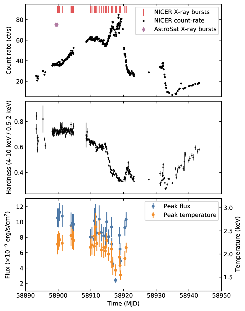
Figure 1: Top: XTE J1739–285 light curve in the $0.5-10\rm\,keV$ energy range, showing one point per NICER pointing. X-ray bursts have been filtered out of the light curve and are indicated with red bars instead. The purple diamonds indicate the times of two X-ray bursts observed with AstroSat (Chakraborty & Banerjee, 2020). Middle: hardness ratio calculated as the $4-10$ keV rate over the $0.5-2$ keV rate. Bottom: peak bolometric flux (left) and peak blackbody temperature (right) for each of the NICER X-ray bursts. Error bars show the 90% confidence region.

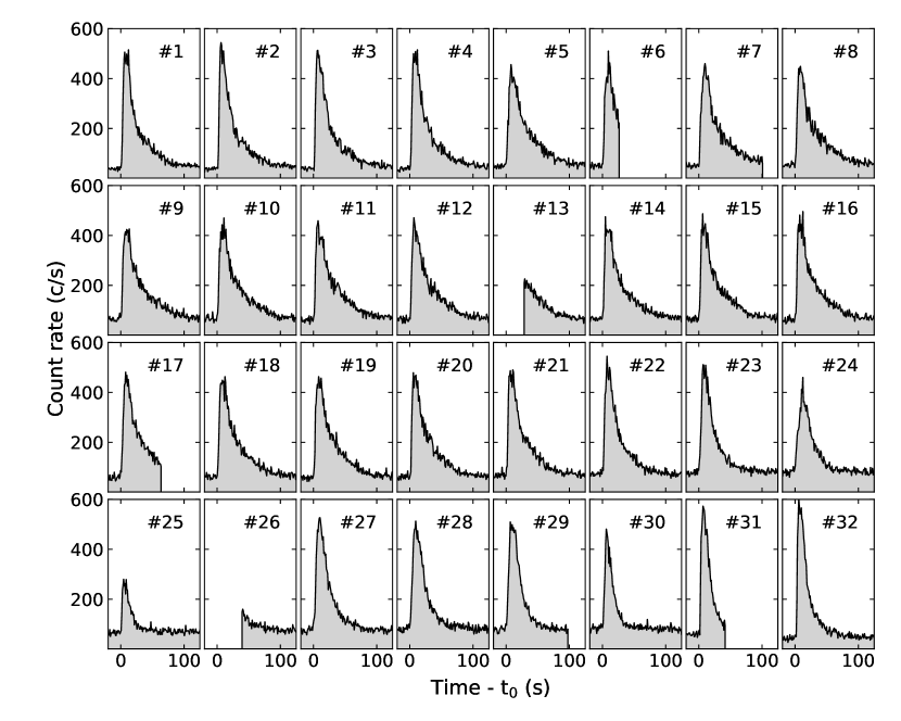
Figure 2: Light curves of each individual X-ray burst from XTE J1739–285 observed with NICER. These light curves are in the $0.5-10\rm\,keV$ energy band, binned at 1-s time resolution, and expressed relative to $t_{0}$, the start time of each respective X-ray burst (see Table 1).

In Figure 2 we show the $0.5-10\rm\,keV$ 1-s light curves of all X-ray bursts relative to their respective onset. The light curve profiles are very similar across all X-ray bursts: the bursts take $5-7\rm\,s$ to rise to a peak rate of about $500\rm\,ct\,\rm\,s^{-1}$ and have duration of approximately $100\rm\,s$. To quantify the shapes of these profiles more precisely, we measured the burst rise time as the interval between the burst onset and the first 1-s light curve bin that was within one standard deviation of the respective burst peak count-rate. We also determined the end time of each X-ray burst by finding the time at which the count-rate decayed back to the preburst level. Specifically, we scanned the 1-s time resolution light curve, starting from $t_{0}+10\rm\,s$, for the first time bin whose count-rate was within $1\sigma$ of the preburst rate. Considering all bursts that decayed before the end of their respective observations, we found an average burst duration of $95\pm 14\rm\,s$.

The similarity between the majority of the X-ray bursts is highlighted in Figure 3, where we show all light curves in the same graph. We see that the bulk of the burst profiles (yellow curves) are highly similar, while the remaining bursts reflect a modest shape evolution across the sample. Specifically, the first four bursts have a sharp rise and higher peak count-rates (purple curves). Similarly, bursts #31 and 32 also peak at higher rates than average, and further show a notably shorter decay (blue curves). Bursts #22, 23, and 26-29 (pink curves) show the same tendency as #31-32, but with less pronounced shifts. Three X-ray bursts are found to show a deviating profile, and are indicated in grey. Burst #24 rises much more slowly to its peak intensity, burst #25 peaks at a much lower rate, and burst #30 decays more rapidly than any of the other bursts in the sample.

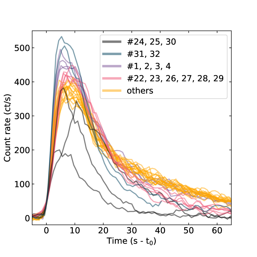
Figure 3: X-ray burst light curves aligned by their start time and with the average pre-burst count-rate subtracted. The X-ray burst profiles show a subtle evolution: the early and late bursts (lower averaged preburst count rate) reach a higher peak rate and show a faster decay as compared to the other X-ray bursts (higher averaged preburst count rates).

3.2 Spectroscopy

We study the spectral properties of the X-ray bursts using xspec version 12.11 (Arnaud, 1996) and version 1.02 of the NICER instrumental response matrix. A background spectrum was generated using version 0.2 of the “environmental” background model (Gendreau et al., in prep). Interstellar absorption was modelled using the Tübingen-Boulder model (tbabs, Wilms et al. 2000).

We first consider the spectral properties of the persistent emission. For each X-ray burst we extracted a spectrum from a $200\rm\,s$ window prior to the burst onset, keeping at least 50 seconds between the end time of the window and the burst onset. In the cases where the burst onset occurred too close to the start of the observation, we instead extracted a persistent emission spectrum after the burst had decayed instead, selecting the 200-s window as close to the end of the observation as possible. In all cases the individual $0.5-10\rm\,keV$ persistent emission spectra could be well described as an absorbed power law. Applying a joint fit to all preburst spectra, we tied the absorption column density across all spectra, but let the power law photon index vary per spectrum. We found the absorption column density at $N_{\text{H}}=\left(1.73\pm 0.01\right)\times 10^{22}\rm\,cm^{-2}$, and a power law photon index that gradually increases with time from $1.5$ to $2$. We measured $0.5-10\rm\,keV$ X-ray flux for each spectrum using the cflux model component, and estimated the bolometric flux by integrating this component between $0.01-100\rm\,keV$. The full set of fit parameters and fluxes are listed in the appendix (Table A1).

We analyzed the burst spectra using a time-resolved approach. We adaptively binned the burst light curves into multiples of 1 second, such that each bin contained at least $500$ counts, yielding about 12 temporal bins per burst. For each bin, we extracted a spectrum and modeled it using an absorbed blackbody superimposed on the persistent emission spectrum, holding all parameters of the persistent emission spectral model fixed at the values listed in Table A1. We also attempted to fit the burst spectra while leaving the normalization of the persistent emission as a free parameter (Worpel et al., 2013); however, this did not improve the fit, and was therefore not pursued further. We further note that none of the X-ray bursts showed evidence for photospheric-radius expansion.

After determining the time-resolved spectral parameters, we fit all burst spectra again to measure the bolometric flux of the burst emission. We multiplied the blackbody component with the cflux model and extrapolated the energy range between $0.01-100\rm\,keV$. Subsequently, we extracted the highest single bin flux and integrated over all time bins in a light curve to measure the bolometric fluence of each burst. The resulting bolometric fluence and peak flux measurements of each burst are listed in Table 1.

In Figure 4 we show the evolution of the spectral parameters for a typical burst from the largest group (#11) along with the evolution measured for burst #32. In each case we see that the burst emission peaks at a blackbody temperature of about $2.5\rm\,keV$, with a bolometric flux of $\approx 1\times 10^{-8}{\rm\,erg{\rm\,s^{-1}}\rm\,cm^{-2}}$. The blackbody emission area peaks about $5-10\rm\,s$ later at $40\,({\rm km/10\,kpc})^{2}$ and $60\,({\rm km/10\,kpc})^{2}$ for bursts #11 and #32, respectively. This evolution pattern is repeated in all X-ray bursts, as illustrated in Figure 5. In this figure we plot the bolometric burst flux and normalization area as a function of blackbody temperature for all X-ray bursts, showing the average per burst-group with a solid line. Here, we see the lag between respective peaks in blackbody temperature and normalization reflected in the curved track traced out in the bottom panel. We further see that there is a gradual evolution in the tracks traced out by these X-ray bursts. Some of this evolution is even more apparent when we consider the peak bolometric flux and peak blackbody temperature as a function of time (see Figure 1). When the source count-rate climbs above $\approx 60\rm\,ct\,\rm\,s^{-1}$ (bolometric flux $\geq 1.4\times 10^{-10}{\rm\,erg{\rm\,s^{-1}}\rm\,cm^{-2}}$), both the peak burst flux and temperature decrease (bursts #22-30).

Finally, we summarize each burst through three standard X-ray burst metrics, as presented in Table 1. We measure the e-folding timescale ($\epsilon$) of the burst tails by modeling the measured bolometric burst flux evolution as an exponential decay. We further determine the $\alpha$ factor, which is the ratio of the persistent fluence between bursts to the fluence of the burst itself

$$\alpha=\frac{F_{\text{preburst}}\Delta t}{E_{\text{burst}}},$$ (1)

where we estimate the persistent fluence by multiplying the preburst flux, $F_{\text{preburst}}$, with the burst recurrence time, $\Delta t$, and $E_{\text{burst}}$ gives the X-ray burst fluence. Finally, we calculate the ratio of the burst fluence to peak burst flux ($\tau$), which represents the equivalent duration of the X-ray burst and gives a rough measure of the burst morphology (van Paradijs et al., 1988). We calculate these metrics only if the measured recurrence time was less than one day, and if the X-ray burst was not truncated.

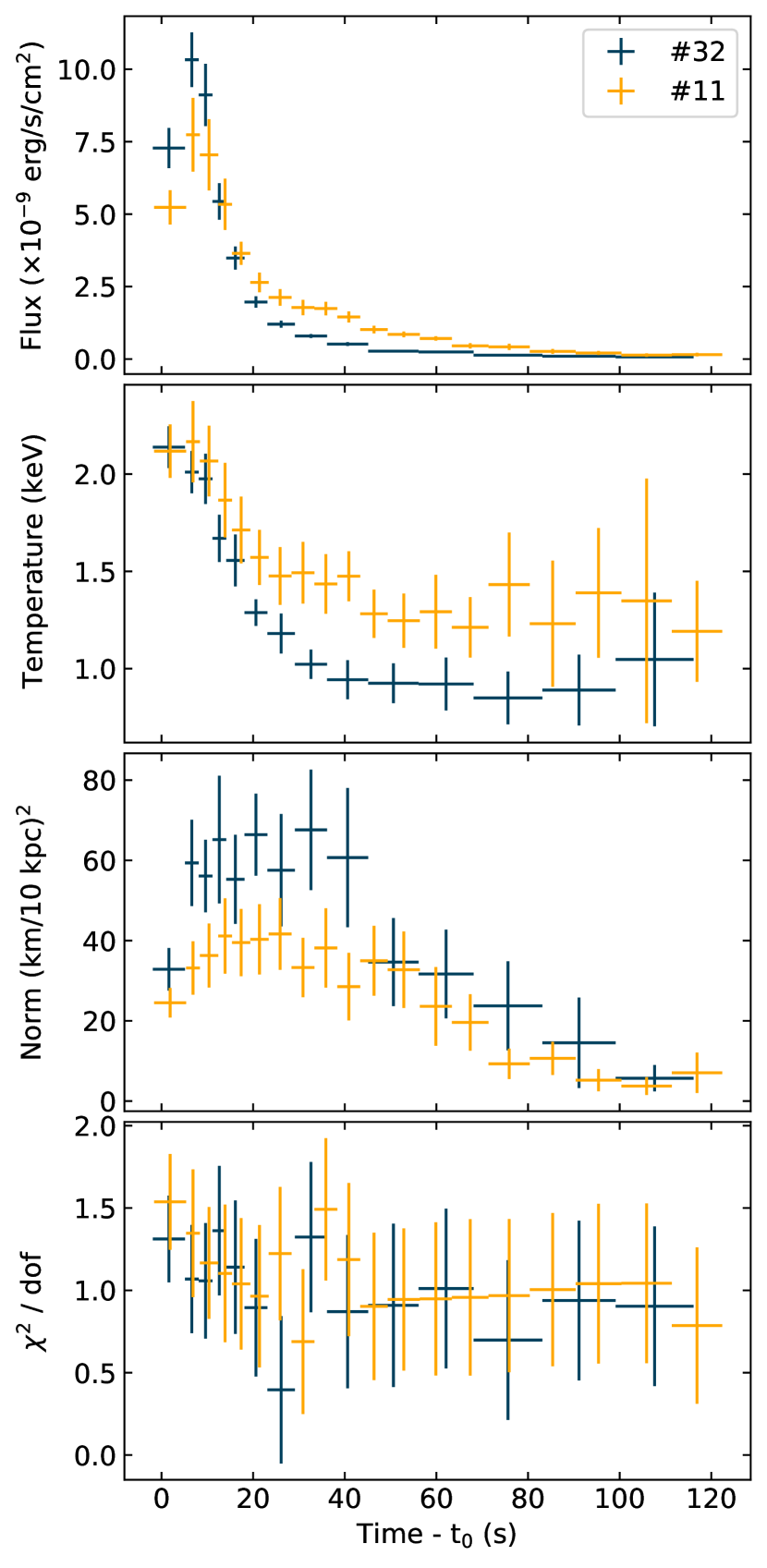
Figure 4: Time resolved spectral fit parameters for X-ray bursts #11 and #32, showing from top to bottom: the bolometric X-ray flux, the blackbody temperature, the blackbody normalization area, and the goodness-of-fit statistic. All vertical error bars show the 90% confidence region, which, for the bottom panel, was derived from the $\chi^{2}$ distribution as $1.645\times\sqrt{2/\text{dof}}$.

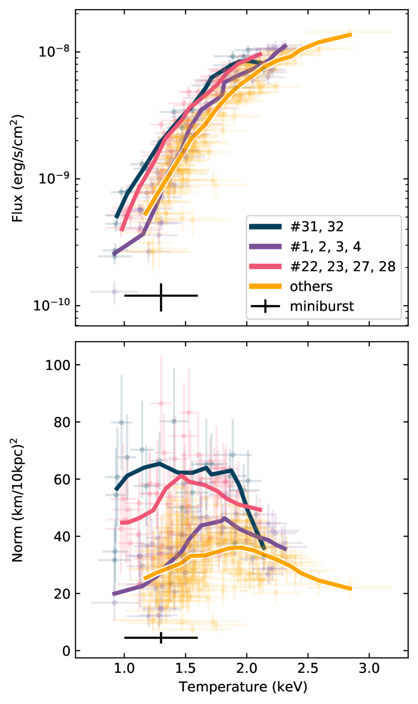
Figure 5: Time resolved spectral fit parameters of all X-ray bursts, showing the bolometric X-ray flux (top), and blackbody normalization (bottom) as a function of blackbody temperature. The solid lines represent the averages for each group. The black point shows the mini-burst, otherwise the color coding is the same as in Figure 3.

3.3 Mini-burst

In ObsID 3050280106 we observed what we will call a mini-burst. At 840 s after the onset of X-ray burst #19, we observed a brief flare-up in count-rate. The event follows the expected profile of an X-ray burst: it has a sharp rise and an approximately exponential decay. In contrast to regular X-ray bursts, however, this mini-burst peaked at 75 ct  s^-1 and lasted only $\approx 30\rm\,s$ (see Figure 6).

We extracted a spectrum for the time interval of the mini-burst and compared it with preburst spectrum #19. Because the mini-burst is comparatively faint, the resulting spectrum is of poor quality and can be successfully fit with several spectral models. The simplest of such models invokes the power law component used to describe the preburst emission, and fits for normalization only. However, the burst-like profile of this event invites an interpretation that is analogous to the spectral model used for the burst emission. If we fix the spectral parameter of the preburst model, then we find that the excess emission is well described by a single-temperature blackbody. The best-fit $\chi^{2}$ is 63 for 61 degrees of freedom, yielding a blackbody temperature of $1.3\pm 0.3\rm\,keV$ with a $0.5-10\rm\,keV$ X-ray flux of $(1.2\pm 0.3)\times 10^{-10}{\rm\,erg{\rm\,s^{-1}}\rm\,cm^{-2}}$. We show this measurement in Figure 5 using a black point, and note that this excess emission is consistent with the flux-temperature relation measured in Section 3.2.

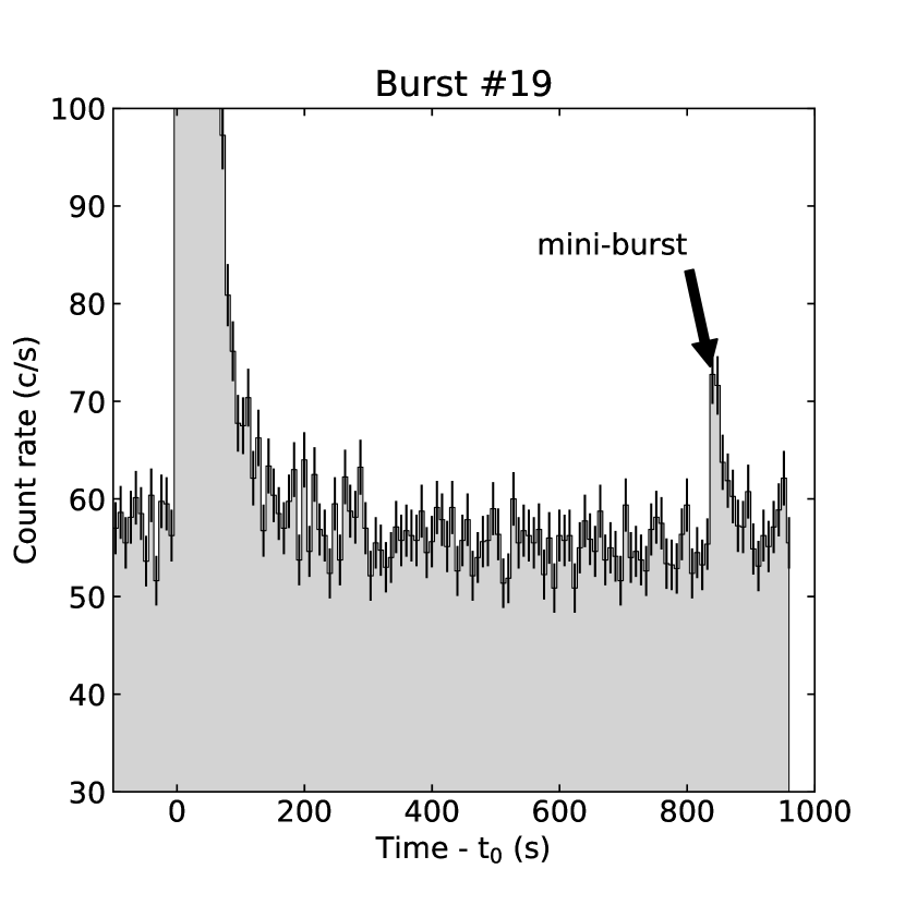
Figure 6: Light curve of the X-ray burst #19 at 8-s time resolution. A mini-burst is observed at $t=840\rm\,s$. Errorbars indicate the $1\sigma$ uncertainty.

3.4 Burst oscillations

We searched the X-ray bursts for the presence of coherent burst oscillations, excluding the mini-burst and burst #29 from the analysis. To avoid confirmation bias towards the 1122 Hz burst oscillation candidate reported by Kaaret et al. (2007), we treated our analysis as a blind search for an unknown oscillation frequency. Hence, we defined our frequency search window to be bounded between $50\rm\,Hz$ and $2000\rm\,Hz$. The lower bound is motivated by the fact that the non-stationary X-ray burst light curve introduces red noise into the power spectrum. For frequencies greater than $50\rm\,Hz$, however, the red noise contribution becomes negligible, and the individual frequency bins are well described by a $\chi^{2}$ distribution (see, e.g. Ootes et al., 2017; Bilous & Watts, 2019). The upper bound on the frequency range is motivated by physical limits on the maximum spin frequency a neutron star can sustain given realistic equation of state constraints (Haensel et al., 2009).

To search for coherent burst oscillations in any given burst, we construct a dynamic power spectrum of the $0.5-10\rm\,keV$ burst light curve using a sliding window method. We apply a window of duration $T$ to a $1/8192\rm\,s$ resolution light curve and then move this window from $t_{0}-10\rm\,s$ to $t_{0}+100\rm\,s$ in steps of $T/2$, where we recall that $t_{0}$ is the burst onset time (as defined in Table 1). For each window position we use the Fourier transform to compute the power density spectrum, and extract the highest measured power. To establish if this measured power is in excess of the noise, we compare it to two approximations of the noise distribution: the $\chi^{2}$ distribution as expected from a pure Poisson counting process; and a numeric simulation of the non-stationary burst light curve.

3.4.1 $\chi^{2}$ statistics

The power spectrum of counting noise is well known to be $\chi^{2}$ distributed (van der Klis, 1989). For any single frequency bin in the power spectrum, we can therefore directly calculate the expected probability that the noise process would yield a power greater than the one measured. For every searched X-ray burst, however, we evaluate the powers in $N_{\text{f}}$ frequency bins for $N_{\text{w}}$ window positions. For simplicity, we treat these $N=N_{\text{f}}\times N_{\text{w}}$ trials as though they are independent. We can then express the chance that the single-trial survival probability $\varepsilon_{1}$ was produced by noise as $\varepsilon_{N}=1-(1-\varepsilon_{1})^{N}$ (see, e.g., Vaughan et al., 1994). When the multi-trial survival probability, $\varepsilon_{N}$, is smaller than $1\%$, we consider the measurement to be a detection at the search level. Finally, we account for the fact that we search 31 different X-ray bursts using multiple search configurations (e.g., different window sizes) by increasing the trial count accordingly.

3.4.2 X-ray burst simulations

A limitation of the $\chi^{2}$ statistics derived from the counting noise process is that it does not account for the fact that the underlying X-ray burst light curve is non-stationary, nor for the fact the overlapping window positions impose correlations between the measured powers. In an effort to more faithfully account for such effects, we also estimate the noise distribution through a series of numeric simulations.

For a given burst, we generate a sample of artificial light curves using an approach similar to that of Bilous & Watts (2019). That is, we wish to generate a list of photon arrival times that follows the slow ($\ll 50\rm\,Hz$) variations in count-rate of an observed burst, but does not contain any high frequency periodic signals. To achieve this, we use the thinning method (Lewis & Shedler, 1979) to generate a realization of a non-homogeneous Poisson process whose underlying rate is specified by a time-continuous light curve. This time-continuous light curve, in turn, is constructed from the real data, through a linear interpolation on the $1/4\rm\,s$ light curve of an observed X-ray burst. In short, this procedure involves four steps:

1. Given the peak count rate, $\lambda_{\text{max}}=600\rm\,ct\,\rm\,s^{-1}$, and burst duration, $T=110\rm\,s$, draw a random number from the Poisson distribution with mean $T\lambda_{\text{max}}$, call this random number $N_{\lambda}$;

2. Draw $N_{\lambda}$ arrival times from a uniform distribution on the burst good time interval $(t_{0}-10,t_{0}+100)$, call them $t_{i}$.

3. Draw $N_{\lambda}$ acceptance/rejection criteria from a uniform distribution on $[0,\lambda_{\text{max}}]$, call them $s_{i}$.

4. Keep only those arrival times with $s_{i}<f(t_{i})$, where $f(\cdot)$ is the continuous time light curve.

For each observed X-ray burst, we simulate a set of 5000 analogous realizations. When applying a search procedure to the real data, we similarly search the simulated data using the same search method, and extract a sample of 5000 ‘highest’ simulated powers. Hence, we directly map out the search-level probability distribution (i.e. adjusted for the $N$ trials in the dynamic power spectrum). Finally, we parameterize each of the resulting distributions into a functional form by fitting it with a log-normal distribution. While the choice for the log-normal is ad hoc, a Kolmogorov-Smirnov test indicates that this model yields a good description (p-value $>0.05$) of the simulated data in every search configuration considered in this paper.

3.4.3 Sliding window searches

We performed a series of sliding window searches on the individual bursts. We selected window durations of $2$, $4$, and $8$ seconds and applied them to the $0.5-10\rm\,keV$ light curves of the bursts. None of these searches yielded a power measurement with a chance probability smaller than the $1\%$ noise probability threshold at the search-level. Hence, no significant burst oscillations were detected.

In a second iteration of searches, we used the same sliding window configuration, and additionally applied a factor 4 binning to the power spectra. This approach is motivated by the fact that burst oscillations may drift in frequency over the course of an X-ray burst, in which case the signal power may be spread out across several frequency bins (see, e.g., Watts, 2012, for a review).

Applying the searches with binning in the frequency domain, we recovered a candidate 386.5 Hz burst oscillation in X-ray burst #2. The candidate signal occurred during the rise of the burst (see Figure 7) and is observed for all three window durations. Based on $\chi^{2}$ statistics, the highest measured power corresponds to a single-trial noise probability of $1.2\times 10^{-12}$. Accounting for the number of trials in all six search configurations (three with, and three without frequency binning), we obtain a multi-trial adjusted noise probability of $1.8\times 10^{-6}$. Further adjusting the trial count to include all 31 X-ray bursts, we obtain $5.6\times 10^{-5}$. Hence, the chance probability that this signal is produced by the counting noise is well below the $1\%$ threshold. Comparing the signal with the numerically estimated noise distribution for X-ray burst #2, we find that the six search configurations have a joint probability of $9\times 10^{-5}$ to produce the observed power by chance. Again extending this analysis to include all 31 X-ray bursts, the total joint noise probability is $2.8\times 10^{-3}$. Hence, the 386.5 Hz signal is again found to be in excess of the noise process, albeit at a lower level of significance.

Given the frequency of the detected burst oscillation in burst #2, we can return to the other bursts to search with higher sensitivity. We repeated all six search procedures, searching only the narrow frequency range from 377 Hz to 397 Hz. This third iteration of searches did not yield any additional detections.

The Leahy normalized power spectrum of a Poisson sampled coherent wave yields a power distribution that is well described as a non-central $\chi^{2}$ distribution (see, e.g., Groth 1975). We write this function as $\overline{\chi}^{2}(P_{\text{m}}|\kappa,\zeta)$, with $P_{\text{m}}$ the measured power, $\kappa$ the degrees of freedom, and $\zeta$ the non-centrality parameter. The latter depends on the signal amplitude, $A$, as

$$\zeta=\frac{\kappa A^{2}}{4N_{\gamma}},$$ (2)

with $N_{\gamma}$ the number of photons. We numerically invert this relation to find the distribution of the signal amplitude given the measured power, and finally express the burst oscillation amplitude as a fractional sinusoidal amplitude relative to the burst flux

$$a=\frac{A}{N_{\gamma}-N_{\text{persistent}}},$$ (3)

where $N_{\text{persistent}}$ gives the number of photons contributed by the persistent emission, as estimated from the preburst count-rate. Using this formalism, we find a fractional amplitude of $a=(26\pm 4)\%$ for the candidate oscillation in burst #2.

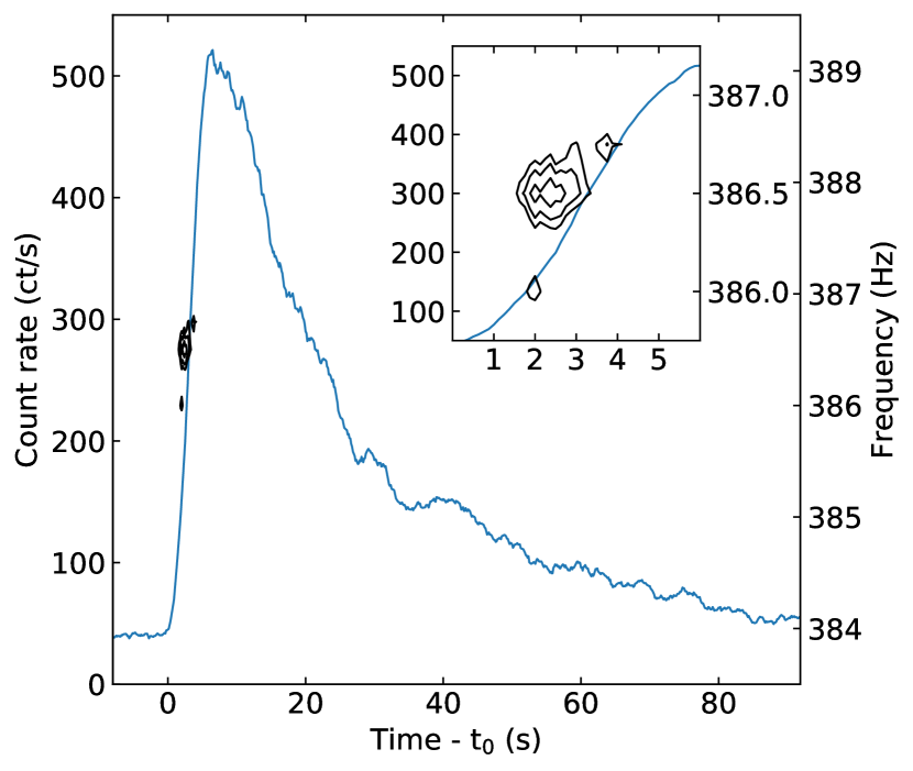
Figure 7: Burst oscillation detection in X-ray burst #2, showing the contours of a dynamic power spectrum (black, right axis), along with the burst light curve (blue, left axis). The contours mark the power (17.4, 21.1, and 26.8) corresponding to the 68%, 95% and 99.7% confidence levels, adjusted for the number of trial frequencies in the spectrum. For illustrative purposes, we oversampled the dynamic power spectrum, i.e., it was calculated using 4 s time windows with steps of 1/8 s. The inset shows the same data, but zoomed-in on the region where the burst oscillation candidate was detected.

4 Discussion

We have presented a spectral and timing analysis of 32 Type I X-ray bursts observed from XTE J1739 with NICER. All X-ray bursts were detected over a 20-day period during which the persistent X-ray emission increased from $4.5\times 10^{-10}{\rm\,erg{\rm\,s^{-1}}\rm\,cm^{-2}}$ to $1\times 10^{-9}{\rm\,erg{\rm\,s^{-1}}\rm\,cm^{-2}}$. This flux range is broadly consistent with the source intensity at which X-ray bursts have been previously reported (Brandt et al., 2005; Kaaret et al., 2007, Section 4.4), and is associated with the hard state of this source (see Section 4.5).

4.1 X-ray burst energetics

The profiles of the X-ray burst light curves are mostly very similar: they take $5-7$ s to rise to their peak intensity, and are followed by an approximately 100 s decay. Such profiles indicate the bursts are due to helium burning in a hydrogen rich environment (see, e.g., Galloway & Keek, 2017, and references therein), with a cooling tail that is governed by the rp-process (Schatz et al., 2001).

Another view of the burst fuel composition is given by the $\alpha$ factor. Due to the relatively short exposures of individual NICER pointings, we did not observe successive bursts in a single uninterrupted exposure, such that all burst recurrence times and $\alpha$ factors listed in Table 1 are formally upper limits. Instead, we estimate the averaged bursting rate by dividing the 226 ks unfiltered exposure collected between the first and last ObsIDs containing an X-ray burst by the number of bursts observed, yielding a recurrence time of $2.0_{-0.3}^{+0.4}\rm\,hr$. If we adopt average values for the burst fluence, persistent flux, and burst waiting time, we find an average $\alpha$ of 47, which is consistent with a mixed hydrogen/helium fuel composition.

If we assume that each X-ray burst depletes the available reservoir of fuel, then $\alpha$ can be predicted from theory as

$$\alpha=\frac{Q_{\text{grav}}}{Q_{\text{nuc}}}(1+z)\frac{\xi_{\text{b}}}{\xi_{\text{p}}},$$ (4)

where $Q_{\text{grav}}=GM_{\text{NS}}/R_{\text{NS}}$ is gravitational potential energy released through accretion, with $G$ the gravitational constant, $M_{\text{NS}}=1.4M_{\odot}$ the neutron star mass, and $R_{\text{NS}}=10\rm\,km$ the neutron star radius. Additionally, $Q_{\text{nuc}}=1.35+6.05\overline{X}\,\mbox{MeV/nucleon}$ (Goodwin et al., 2019) is the nuclear energy generation rate in a burning layer with averaged hydrogen fraction, $\overline{X}$, and $(1+z)=1.31$ gives the gravitational redshift factor. Finally, $\xi_{\text{p}}$ and $\xi_{\text{b}}$ give the anisotropy factors for the persistent and burst emission, respectively. Given the observed $\alpha$ and an allowed range for hydrogen abundance of $0.1<\overline{X}<0.7$, we find that the ratio of anisotropy factors, $\xi_{\text{b}}/\xi_{\text{p}}$, is in the range $0.3-0.9$. If we adopt a simple thin disk model, then we can relate these anisotropy factors to the system inclination (Fujimoto, 1988; He & Keek, 2016), such that the allowed system inclination is $65\arcdeg<i<90\arcdeg$. Hence, the bursting properties suggest that XTE J1739 is a relatively high inclination system. The lack of eclipses in the light curve further indicates that we are not viewing the system edge-on, allowing for an upper limit on the inclination of $i\lesssim 75\arcdeg$ (Frank et al., 1987).

4.2 Burst light curve variations

While the majority of observed bursts are very similar, some evolution in the burst light curve shapes can be observed across the sample. This is demonstrated in Figure 3, where we grouped the burst light curves by shape. Relative to the most commonly observed burst shape (yellow), we selected three groups of burst shapes that each tend toward higher peak count-rates and shorter decay tails (blue, purple, pink). In addition to exhibiting similar burst profiles, these bursts share commonalities in time and persistent flux as well. The bursts of the first group (#1-4; purple curves) occur early in the outburst and have the lowest bolometric persistent fluxes of the sample ($8\times 10^{-10}{\rm\,erg{\rm\,s^{-1}}\rm\,cm^{-2}}$). Those in the second group (#22-29, pink curves) have the highest persistent fluxes in the sample ($1.5-1.8\times 10^{-9}{\rm\,erg{\rm\,s^{-1}}\rm\,cm^{-2}}$), and coincide with a notable drop in peak burst temperature and peak burst flux (Figure 1). Finally, the third group bursts (#31, 32) have the sharpest profiles of the observed bursts, and occur right after the X-ray flux dropped back down to $1\times 10^{-9}{\rm\,erg{\rm\,s^{-1}}\rm\,cm^{-2}}$.

The observed pivot in burst shape from longer burst with lower peak rates to shorter bursts with higher peak rates is not uncommon and can be attributed to change in fuel composition, with sharper bursts having a comparatively higher helium abundance (Lewin et al., 1993; Galloway & Keek, 2017). Some evidence that this effect is at play in XTE J1739 can be found in the $\alpha$ factors. Considering the $\alpha$ factors of those bursts with the most robust recurrence times, we find values ranging from about 40 (#12,14) to 80 (#29) and 134 (#30), suggesting that the bursts with sharper profiles indeed have a lower hydrogen content.

What physical process is driving fuel composition changes in XTE J1739 is less clear. The most likely driver of such evolution is the changing mass accretion rate (e.g., Bildsten, 1998). However, the most common burst shape has the longest tails, and thus the highest hydrogen content. Relative to this group, we see that the hydrogen content decreases for both increasing and decreasing mass accretion rates.

4.3 Short-recurrence bursts

A caveat to the interpretation of $\alpha$ is that at least some of the X-ray bursts do not appear to exhaust the fuel layer. Given its light curve profile and short waiting time relative to burst #19, the mini-burst reported in section 3.3 is most likely a short-recurrence burst (see, e.g., Keek et al., 2010). Such bursts occur with recurrence times that are too short for the accretion process to fully replenish the stellar atmosphere, and are therefore fuelled by left-over hydrogen and helium on the stellar surface.

If the mini-burst is indeed a short-recurrence burst, then it seems likely that X-ray burst #25 was also a short recurrence event. This burst occurred 480 s into its respective pointing, and is preceded by a 6 hr gap in coverage. Given that the burst recurrence time is on the order of 2 hours, we almost assuredly missed the X-ray bursts directly preceding burst #25.

In a similar vein, we can also consider bursts #24 and #30 in the context of short recurrence events. Each of these two bursts were less energetic than the remaining sample, albeit not to the extent of burst #25. If these bursts only burned some fraction of the available fuel, that would account for their reduced intensity, while leaving requisite material behind for short recurrence bursts (Keek et al., 2010; Keek & Heger, 2017). Hence, we can speculate that bursts #24 and #30 were primary events of short recurrence trains. These bursts were followed by only 7 and 9 minutes of exposure before a 66 and 78 minute data gap, respectively. The data sampling therefore leaves sufficient space for such short recurrence events to have occurred. This interpretation is complicated by the slow rise of burst #24, as the process that governed this slow rise might also underpin the reduced intensity. It is not clear what causes this slow rise, although we note that ignition latitude has been linked to the rise morphology (Maurer & Watts, 2008).

4.4 The MINBAR sample

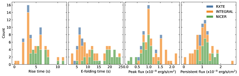
Figure 8: Stacked histograms of X-ray burst properties measured with NICER versus those reported in MINBAR.

Most of the X-ray bursts observed with NICER appear to have an appreciable hydrogen content. This stands in contrast with the X-ray bursts observed with RXTE, which were all reported to be typical helium-fueled bursts (Kaaret et al., 2007; Galloway et al., 2008). This raises the question if the bursting regime sampled with NICER is somehow different than the bursting phases observed previously. To investigate this question, we compare some of the burst statistics obtained with NICER to those reported in MINBAR (Galloway et al., 2020). In Figure 8 we show histograms of the burst rise time, e-folding time, peak burst flux and the persistent flux. Each is color coded per observatory (blue for RXTE, orange for INTEGRAL, and green for NICER). We see that some systematic shifts are apparent: the NICER bursts appear to show a slower rise and longer decay than the RXTE and INTEGRAL bursts. The NICER peak fluxes are slightly lower, while the flux of the persistent accretion is marginally higher. On the whole, however, the MINBAR and NICER samples are not dramatically different.

4.5 Spectral state

To place our observations in the context of the source state and accretion rate evolution, we constructed a hardness intensity diagram from the light curve data described in Section 3.1 (Figure 9). That is, we calculated the hardness ratio as the $4-10\rm\,keV$ count rate over the $0.5-2\rm\,keV$ count rate and adopted the full band ($0.5-10\rm\,keV$) rate for the intensity, averaging the data per continuous pointing. In addition to the bursting epoch observations, we also included the NICER data collected in August 2019 (Bult et al., 2019b), which covered higher intensities (count-rates $>100\rm\,ct\,\rm\,s^{-1}$). The X-ray bursts are clearly observed along a hard state track. Toward the highest persistent accretion rates of the bursting epoch, however, the source may have transitioned to an intermediate state.

Considering the time-evolution of the source intensity and hardness, as shown in Figure 1, we see that the highest observed count-rates occur after a rapid drop in hardness. Coincident with this apparent spectral shift, the X-ray bursts show a decrease in their peak bolometric flux and peak blackbody temperature. What causes this apparent change in burst character is not obvious, but it might be explained by a change in the accretion state.

One possibility is that a change in the accretion disk structure is affecting the anisotropy ratio. For instance, the formation of a surface boundary layer could cause more of the burst emission to be shadowed out by accretion flow, thus lowering the observed burst flux. Such shadowing, however, is predicted to cause a hardening of the burst spectrum (Suleimanov et al., 2012; Kajava et al., 2014), which is opposite to what we observe.

Alternatively, the decrease in burst flux and temperature might be related to the presence of short-recurrence bursts. When short-recurrence bursts occur, they change the fuel layer, and alter ignition conditions of long-duration bursts as well (Keek & Heger, 2017). Possibly this effect is what drives the depression in the peak burst flux and temperature. This scenario is compatible with our data, as all candidate short-recurrence bursts discussed Section 4.3 occur during this short time interval where the count-rate is high and the hardness is low. Furthermore, surveys of X-ray bursters show that short-recurrence bursts often only occur in a comparatively narrow range of luminosity just below the transition to the soft state (Keek et al., 2010).

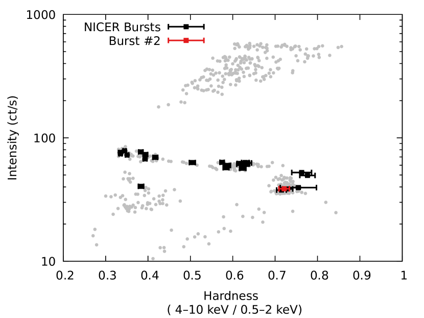
Figure 9: Hardness-intensity diagram for XTE J1739, showing one data point for each continuous NICER pointing in grey. We further highlight those pointings containing an X-ray burst in black, and show burst #2 in red. For visual clarity we show the $1\sigma$ error bars for the highlighted points only.

To estimate the source mass accretion rate during the bursting epoch, we adopt a source distance of $4_{-2}^{+4}$ kpc, as derived from Gaia parallax measurements (Bailer-Jones et al., 2018). Assuming a 1.4 solar mass neutron star with a 10 km radius, the measured bolometric persistent flux implies a mass accretion rate of $\dot{M}\approx 2\times 10^{-10}\,M_{\odot}\rm\,yr^{-1}$, or about 1.5% of the Eddington rate. This accretion rate is lower than the $\approx 10\%$ Eddington rate expected based on the burst behavior (Galloway et al., 2008; Galloway & Keek, 2017). While discrepancies between the accretion rate inferred from the X-ray luminosity and the burst physics are not uncommon (see, e.g., Cornelisse et al., 2003), there are additional caveats to this comparison. First, the Gaia distance is likely an underestimate. As noted by Galloway et al. (2020), the distance is derived using a probabilistic method that is weighted on the distribution of matter in the galaxy. Because LMXBs are likely more concentrated toward the galactic center than the stellar population, however, the resulting Gaia distance is likely biased. Second, in estimating the accretion rate, we did not account for the anisotropy associated with the system inclination. The $\alpha$ factor indicates that we are likely viewing the binary at very high inclination, such that accretion luminosity is preferentially beamed away from the line of sight. Thus, the accretion rate onto the neutron star is likely higher than inferred.

4.6 Stellar spin frequency

We searched 31 of the observed X-ray bursts for a presence of burst oscillations, finding one candidate signal at a frequency of 386.5 Hz. With a single trial probability of $10^{-12}$, the detected signal deviates significantly from the expected noise distribution. After accounting for all frequencies tested across all bursts, we conservatively estimated the multi-trial adjusted probability at $2.8\times 10^{-3}$.

The signal was detected only after binning the power spectra by a factor of four, suggesting that the underlying oscillation had a drifting frequency. Considering the sub-threshold detections around the peak power shows weak evidence that the signal is drifting by about 1 Hz in the $\approx 2\rm\,s$ period that the power is highest. Considering that the candidate detection occurs during the rising slope of X-ray burst #2, such a drift in frequency would be in line with known behaviors of burst oscillations (see, e.g., Watts, 2012).

The fractional amplitude of the signal is measured at $26\pm 4\%$. While such an amplitude is plausible from theoretical considerations (Mahmoodifar & Strohmayer, 2016), the observational record indicates that it is comparatively large (Ootes et al., 2017; Galloway et al., 2020). While rising phase burst oscillations have systematically larger amplitudes than cooling tail oscillations, the amplitude also depends on the accretion rate. Similarly strong oscillations are normally observed only in the soft state (Ootes et al., 2017; Galloway et al., 2020). In contrast, the burst oscillation candidate detected in this work occurred in the hard state.

In addition to showing different amplitudes, the detectability of burst oscillations also depends on the source spectral state. Burst oscillations can occur at any accretion rate, however the fraction of bursts that show such oscillations has been found to be much higher in the soft state than in the hard state (Muno et al., 2004; Ootes et al., 2017; Galloway et al., 2020). This tendency may go some way to explain why we only detected one candidate signal out of 31 analyzed bursts. A caveat, however, is that all known systematics of burst oscillations are derived entirely from observations made with RXTE, and thus based on an higher energy passband than that of NICER. A limited number of burst oscillation detections made with NICER (Mahmoodifar et al., 2019; Bult et al., 2019a) do not yet point to dramatically different behavior at lower energies. Instead, because the burst oscillation amplitudes increase with photon energy, it appears to be more challenging to observe these signals with NICER than it was with RXTE. This energy dependence might also play a role in explaining why the 386.5 Hz signal was only detected in a single X-ray burst.

While the 386.5 Hz burst oscillation candidate deviates significantly from the noise distribution, it is only observed in a single independent time-frame and does not repeat in any of the other bursts. So, while all observed characteristics make it a plausible burst oscillation, we caution that this signal should be treated as a candidate until it can be independently confirmed. Even with all noted caveats, it is worth stressing that the 386.5 Hz signal reported here is more prominent than the 1122 Hz oscillation candidate reported by Kaaret et al. (2007), which had a single trial probability of $5\times 10^{-10}$. The ratio of the two frequencies is 2.9, so it is possible that the two signals are harmonically related. However, given that such a relation prefers a fundamental frequency smaller than 386.5 Hz and that burst oscillations tend to appear at or below the underlying spin frequency (Watts, 2012), such an interpretation does not appear probable. Either way, based on the NICER observations presented here, it seems unlikely that XTE J1739 has a sub-millisecond spin period.

Appendix A Spectroscopy

Table A1: Preburst spectral parameters

Burst	$N_{\text{H}}$	Photon Index	X-ray Flux	Bol. Flux	$\chi^{2}$/bins
	($\times 10^{22}$  cm-2)		($\times 10^{-9}{\rm\,erg{\rm\,s^{-1}}\rm\,cm^{-2}}$)	($\times 10^{-9}{\rm\,erg{\rm\,s^{-1}}\rm\,cm^{-2}}$)
1	$1.73\pm 0.01$	$1.49\pm 0.04$	$0.451\pm 0.010$	$0.77\pm 0.02$	253.96 / 200
2		$1.50\pm 0.04$	$0.464\pm 0.010$	$0.79\pm 0.02$	170.85 / 197
3		$1.48\pm 0.04$	$0.460\pm 0.010$	$0.78\pm 0.02$	209.59 / 195
4		$1.48\pm 0.07$	$0.457\pm 0.016$	$0.78\pm 0.03$	094.70 / 079
5		$1.45\pm 0.04$	$0.585\pm 0.013$	$1.00\pm 0.03$	164.74 / 184
6		$1.48\pm 0.04$	$0.586\pm 0.011$	$1.00\pm 0.02$	239.28 / 238
7		$1.52\pm 0.04$	$0.611\pm 0.011$	$1.03\pm 0.02$	254.14 / 254
8		$1.45\pm 0.05$	$0.631\pm 0.016$	$1.08\pm 0.04$	130.10 / 141
9		$1.62\pm 0.06$	$0.768\pm 0.022$	$1.27\pm 0.04$	095.82 / 106
10		$1.61\pm 0.03$	$0.762\pm 0.012$	$1.27\pm 0.02$	295.87 / 291
11		$1.64\pm 0.03$	$0.733\pm 0.012$	$1.21\pm 0.02$	285.46 / 287
12		$1.63\pm 0.03$	$0.739\pm 0.012$	$1.23\pm 0.02$	317.18 / 286
13		$1.60\pm 0.03$	$0.732\pm 0.012$	$1.22\pm 0.02$	254.77 / 276
14		$1.62\pm 0.03$	$0.747\pm 0.012$	$1.24\pm 0.02$	280.75 / 289
15		$1.71\pm 0.03$	$0.755\pm 0.012$	$1.25\pm 0.02$	331.93 / 292
16		$1.65\pm 0.03$	$0.727\pm 0.012$	$1.20\pm 0.02$	311.73 / 283
17		$1.65\pm 0.03$	$0.719\pm 0.012$	$1.19\pm 0.02$	288.83 / 283
18		$1.67\pm 0.03$	$0.702\pm 0.012$	$1.16\pm 0.02$	274.24 / 274
19		$1.63\pm 0.04$	$0.684\pm 0.013$	$1.13\pm 0.02$	206.22 / 218
20		$1.68\pm 0.04$	$0.686\pm 0.011$	$1.13\pm 0.02$	254.35 / 272
21		$1.83\pm 0.04$	$0.742\pm 0.012$	$1.24\pm 0.02$	321.53 / 286
22		$1.99\pm 0.03$	$0.833\pm 0.013$	$1.46\pm 0.03$	324.82 / 288
23		$2.05\pm 0.03$	$0.866\pm 0.014$	$1.57\pm 0.04$	263.70 / 293
24		$2.07\pm 0.05$	$0.929\pm 0.020$	$1.70\pm 0.06$	153.40 / 191
25		$2.05\pm 0.04$	$0.839\pm 0.014$	$1.52\pm 0.04$	289.66 / 295
26		$2.08\pm 0.03$	$0.860\pm 0.014$	$1.58\pm 0.05$	302.44 / 293
27		$2.14\pm 0.03$	$0.864\pm 0.015$	$1.65\pm 0.05$	250.30 / 287
28		$2.14\pm 0.03$	$0.894\pm 0.016$	$1.78\pm 0.06$	350.75 / 295
29		$1.97\pm 0.02$	$1.026\pm 0.012$	$1.79\pm 0.03$	427.82 / 433
30		$2.14\pm 0.03$	$0.954\pm 0.016$	$1.82\pm 0.06$	275.86 / 301
31		$2.12\pm 0.04$	$0.554\pm 0.011$	$1.04\pm 0.04$	266.98 / 222
32		$2.07\pm 0.04$	$0.469\pm 0.010$	$0.86\pm 0.03$	240.30 / 201

References

- Arnaud (1996) Arnaud, K. A. 1996, in Astronomical Society of the Pacific Conference Series, Vol. 101, Astronomical Data Analysis Software and Systems V, ed. G. H. Jacoby & J. Barnes, 17
- Bailer-Jones et al. (2018) Bailer-Jones, C. A. L., Rybizki, J., Fouesneau, M., Mantelet, G., & Andrae, R. 2018, AJ, 156, 58
- Bildsten (1998) Bildsten, L. 1998, in NATO ASI Series, Vol. 515, The Many Faces of Neutron Stars, ed. R. Buccheri, J. van Paradijs, & A. Alpar, 419
- Bilous & Watts (2019) Bilous, A. V., & Watts, A. L. 2019, ApJS, 245, 19
- Bodaghee et al. (2005) Bodaghee, A., Mowlavi, N., Kuulkers, E., et al. 2005, The Astronomer’s Telegram, 592, 1
- Bozzo et al. (2020) Bozzo, E., Sanchez-Fernandez, C., Ferrigno, C., et al. 2020, The Astronomer’s Telegram, 13483, 1
- Brandt et al. (2005) Brandt, S., Kuulkers, E., Bazzano, A., et al. 2005, The Astronomer’s Telegram, 622, 1
- Bult et al. (2020) Bult, P., Chakrabarty, D., Arzoumanian, Z., et al. 2020, ApJ, 898, 38
- Bult et al. (2019a) Bult, P., Jaisawal, G. K., Güver, T., et al. 2019a, ApJ, 885, L1
- Bult et al. (2019b) Bult, P. M., Gendreau, K. C., Strohmayer, T. E., et al. 2019b, The Astronomer’s Telegram, 13148, 1
- Chakraborty & Banerjee (2020) Chakraborty, S., & Banerjee, S. 2020, The Astronomer’s Telegram, 13538, 1
- Chenevez et al. (2006) Chenevez, J., Shaw, S. E., Kuulkers, E., et al. 2006, The Astronomer’s Telegram, 734, 1
- Cornelisse et al. (2003) Cornelisse, R., in’t Zand, J. J. M., Verbunt, F., et al. 2003, A&A, 405, 1033
- Frank et al. (1987) Frank, J., King, A. R., & Lasota, J. P. 1987, A&A, 178, 137
- Fujimoto (1988) Fujimoto, M. Y. 1988, ApJ, 324, 995
- Galloway & Keek (2017) Galloway, D. K., & Keek, L. 2017, arXiv e-prints, arXiv:1712.06227
- Galloway et al. (2008) Galloway, D. K., Muno, M. P., Hartman, J. M., Psaltis, D., & Chakrabarty, D. 2008, ApJS, 179, 360
- Galloway et al. (2020) Galloway, D. K., in’t Zand, J., Chenevez, J., et al. 2020, ApJS, 249, 32
- Gendreau & Arzoumanian (2017) Gendreau, K., & Arzoumanian, Z. 2017, Nature Astronomy, 1, 895
- Goodwin et al. (2019) Goodwin, A. J., Heger, A., & Galloway, D. K. 2019, ApJ, 870, 64
- Groth (1975) Groth, E. J. 1975, ApJS, 29, 285
- Haensel et al. (2009) Haensel, P., Zdunik, J. L., Bejger, M., & Lattimer, J. M. 2009, A&A, 502, 605
- He & Keek (2016) He, C. C., & Keek, L. 2016, ApJ, 819, 47
- Kaaret et al. (2007) Kaaret, P., Prieskorn, Z., in ’t Zand, J. J. M., et al. 2007, ApJ, 657, L97
- Kajava et al. (2014) Kajava, J. J. E., Nättilä, J., Latvala, O.-M., et al. 2014, MNRAS, 445, 4218
- Keek et al. (2010) Keek, L., Galloway, D. K., in’t Zand, J. J. M., & Heger, A. 2010, ApJ, 718, 292
- Keek & Heger (2017) Keek, L., & Heger, A. 2017, ApJ, 842, 113
- Lewin et al. (1993) Lewin, W. H. G., van Paradijs, J., & Taam, R. E. 1993, Space Sci. Rev., 62, 223
- Lewis & Shedler (1979) Lewis, P. A. W., & Shedler, G. S. 1979, Naval Research Logistics Quarterly, 26, 403
- Mahmoodifar & Strohmayer (2016) Mahmoodifar, S., & Strohmayer, T. 2016, ApJ, 818, 93
- Mahmoodifar et al. (2019) Mahmoodifar, S., Strohmayer, T. E., Bult, P., et al. 2019, ApJ, 878, 145
- Markwardt et al. (1999) Markwardt, C. B., Marshall, F. E., Swank, J. H., & Wei, C. 1999, IAU Circ., 7300, 1
- Maurer & Watts (2008) Maurer, I., & Watts, A. L. 2008, MNRAS, 383, 387
- Mereminskiy & Grebenev (2019) Mereminskiy, I. A., & Grebenev, S. A. 2019, The Astronomer’s Telegram, 13138, 1
- Muno et al. (2004) Muno, M. P., Galloway, D. K., & Chakrabarty, D. 2004, ApJ, 608, 930
- Ootes et al. (2017) Ootes, L. S., Watts, A. L., Galloway, D. K., & Wijnands, R. 2017, ApJ, 834, 21
- Sanchez-Fernandez et al. (2012) Sanchez-Fernandez, C., Chenevez, J., Pavan, L., et al. 2012, The Astronomer’s Telegram, 4304, 1
- Sanchez-Fernandez et al. (2020) Sanchez-Fernandez, C., Ferrigno, C., Bozzo, E., et al. 2020, The Astronomer’s Telegram, 13473, 1
- Savitzky & Golay (1964) Savitzky, A., & Golay, M. J. E. 1964, Analytical Chemistry, 36, 1627
- Schatz et al. (2001) Schatz, H., Aprahamian, A., Barnard, V., et al. 2001, Phys. Rev. Lett., 86, 3471
- Shaw et al. (2005) Shaw, S. E., Kuulkers, E., Oosterbroek, T., et al. 2005, The Astronomer’s Telegram, 615, 1
- Suleimanov et al. (2012) Suleimanov, V., Poutanen, J., & Werner, K. 2012, A&A, 545, A120
- van der Klis (1989) van der Klis, M. 1989, in NATO ASI Series, Vol. 262, Timing Neutron Stars, ed. H. Ögelman & E. P. J. van den Heuvel (Dordrecht: Kluwer), 27
- van Paradijs et al. (1988) van Paradijs, J., Penninx, W., & Lewin, W. H. G. 1988, MNRAS, 233, 437
- Vaughan et al. (1994) Vaughan, B. A., van der Klis, M., Wood, K. S., et al. 1994, ApJ, 435, 362
- Watts (2012) Watts, A. L. 2012, ARA&A, 50, 609
- Wilms et al. (2000) Wilms, J., Allen, A., & McCray, R. 2000, ApJ, 542, 914
- Worpel et al. (2013) Worpel, H., Galloway, D. K., & Price, D. J. 2013, ApJ, 772, 94