An Energy-Stable Parametric Finite Element Method for Simulating Solid-state Dewetting Problems in Three Dimensions

Abstract

We propose an accurate and energy-stable parametric finite element method for solving the sharp-interface continuum model of solid-state dewetting in three-dimensional space. The model describes the motion of the film/vapor interface with contact line migration and is governed by the surface diffusion equation with proper boundary conditions at the contact line. We present a weak formulation for the problem, in which the contact angle condition is weakly enforced. By using piecewise linear elements in space and backward Euler method in time, we then discretize the formulation to obtain a parametric finite element approximation, where the interface and its contact line are evolved simultaneously. The resulting numerical method is shown to be well-posed and unconditionally energy-stable. Furthermore, the numerical method is generalized to the case of anisotropic surface energies in the Riemannian metric form. Numerical results are reported to show the convergence and efficiency of the proposed numerical method as well as the anisotropic effects on the morphological evolution of thin films in solid-state dewetting.

4H15, 74S05, 74M15, 65Z99

1 Introduction

A thin solid film deposited on the substrate will agglomerate or dewet to form isolated islands due to surface tension/capillarity effects when heated to high enough temperatures but well below the thin film’s melting point. This process is referred to as the solid-state dewetting (SSD) [1] since the thin film remains solid. In recent years, SSD has been found wide applications in thin film technologies, and it is emerging as a promising route to produce well-controlled patterns of particle arrays used in sensors [2], optical and magnetic devices [3], and catalyst formations [4]. A lot of experimental (e.g., [5, 6, 7, 8, 9, 10, 11]) and theoretical efforts (e.g., [12, 13, 14, 15, 16, 17, 18, 19, 20, 21]) have been devoted to SSD not just because of its importance in industrial applications but also the arising scientific questions within the problem.

In general, SSD can be regarded as a type of open surface evolution problem governed by surface diffusion [22] and moving contact lines [23]. When the thin film moves along the solid substrate, a moving contact line forms where the three phases (i.e., solid film, vapor and substrate) meet. This brings an additional kinetic feature to this problem. Recently, different mathematical models and simulation methods have been proposed to study SSD, such as sharp-interface models [23, 19, 14, 24], phase-field models [12, 25, 26, 27] and other models including the crystalline formulation [28, 29], discrete chemical potential method [18] and kinetic Monte Carlo method [30].

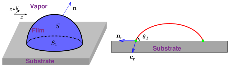
Figure 1: Left panel: A geometric setup of SSD, where a thin film (shaded in blue) is deposited on a flat rigid substrate (shaded in gray), $S$ is the film/vapor interface and $S_{1}$ is the film/substrate interface. Right panel: configuration of the contact angle: $\theta_{d}=\cos^{-1}(\mathbf{c}_{{}_{\Gamma}}\cdot\mathbf{n}_{{}_{\Gamma}})$ at the contact line (green).

In this work, we will restrict ourselves to the model in [24]. It is a sharp-interface model in three dimensions (3D) and was developed based on the thermodynamic variation. As illustrated in Fig. 1(a), we consider the case when a thin film is deposited on a flat substrate. The evolving film/vapor interface is described by a moving open surface $S(t)$ with mapping given by (with $\mathbf{X}=(x,~{}y,~{}z)^{T}$ or $\mathbf{X}=(x_{1},~{}x_{2},~{}x_{3})^{T}$)

$$\mathbf{X}(\mbox{\boldmath{$\rho$}},~{}t)=\Bigl{(}x_{1}(\mbox{\boldmath{$\rho$}},t),~{}x_{2}(\mbox{\boldmath{$\rho$}},~{}t),~{}x_{3}(\mbox{\boldmath{$\rho$}},t)\Bigr{)}^{T}:\,S^{0}\times[0,~{}T]\to\mathbb{R}^{3},$$ (1)

where $S^{0}=S(0)$ is the initial surface. The film/substrate interface is a flat surface, i.e., a two-dimensional moving domain and denoted by $S_{1}(t)$. The two interfaces intersect at the contact line and form a closed curve $\Gamma(t):=S(t)\cap S_{1}(t)$. We assume $\Gamma(t)$ is a simple closed curve and positively orientated with the mapping given by: $\Gamma(t):=\mathbf{X}_{{}_{\Gamma}}(\mbox{\boldmath{$\rho$}},~{}t),\;\mbox{\boldmath{$\rho$}}\in\Gamma^{0}=\Gamma(0).$

Some relevant geometric parameters are defined as follows: $\mathbf{n}$ and $\mathcal{H}$ are the unit outward normal vector and mean curvature of $S(t)$, respectively; $\mathbf{c}_{{}_{\Gamma}}$ and $\mathbf{n}_{{}_{\Gamma}}$ represent the outward unit conomral vector of $S(t)$ and $S_{1}(t)$, respectively, and $\nabla_{s}$ is the surface gradient operator defined in (64). The sharp-interface model of SSD in 3D can be stated as [24]:

$$\partial_{t}\mathbf{X}=\Delta_{s}\mathcal{H}\;\mathbf{n},$$ (2a)

$$\mathcal{H}=-\left(\Delta_{s}{\mathbf{X}}\right)\cdot\mathbf{n},$$ (2b)

where $\Delta_{s}=\nabla_{s}\cdot\nabla_{s}$ is the surface Laplacian operator. The above equations are supplemented with the following conditions at $\Gamma(t)$:

(i) The contact line condition

$$x_{3}(\cdot,~{}t)|_{{}_{\Gamma}}=0,\qquad t\geq 0.$$ (3a)

(ii) The relaxed contact angle condition

$$\partial_{t}\mathbf{X}_{{}_{\Gamma}}=-\eta\left(\mathbf{c}_{{}_{\Gamma}}\cdot\mathbf{n}_{{}_{\Gamma}}-\cos\theta_{Y}\right)\,\mathbf{n}_{{}_{\Gamma}},\qquad t\geq 0.$$ (3b)

(iii) The zero-mass flux condition

$$\left.\left(\mathbf{c}_{{}_{\Gamma}}\cdot\nabla_{s}\mathcal{H}\right)\right|_{{}_{\Gamma}}=0,\qquad t\geq 0.$$ (3c)

Here $\theta_{Y}$ is the Young’s equilibrium angle, and $\eta>0$ is the contact line mobility which controls the relaxation rate of the dynamical contact angles to the equilibrium contact angle. Condition (i) ensures that the contact line always move along the substrate surface. When $\eta\to\infty$, condition (ii) collapses to the well-known Young’s equation. Condition (iii) implies that there is no mass-flux at the contact line thus the total mass/volume of the thin film is conserved.

The total free energy of the system consists of the film/vapor interfacial energy and the substrate surface energy:

$$W(t):=|S(t)|-\cos\theta_{Y}\,|S_{1}(t)|,$$ (4)

where $|S(t)|$ and $|S_{1}(t)|$ denote the surface area of $S(t)$ and $S_{1}(t)$, respectively. Let $\Omega(t)$ be the region enclosed by $S(t)$ and $S_{1}(t)$, then the dynamic system obeys the conservation law for the total volume (mass) and the dissipation law for the total surface energy [24]

$$\frac{\mathrm{d}}{\mathrm{d}t}|\Omega(t)|=\int_{S(t)}\Delta_{s}\mathcal{H}\,\mathrm{d}A\equiv 0,\qquad t\geq 0,$$ (5a)

$$\frac{\mathrm{d}}{\mathrm{d}t}W(t)=-\int_{S(t)}\left\lVert\nabla_{s}\mathcal{H}\right\rVert^{2}\;\mathrm{d}A-\eta\int_{\Gamma(t)}\left(\mathbf{c}_{{}_{\Gamma}}\cdot\mathbf{n}_{{}_{\Gamma}}-\cos\theta_{Y}\right)^{2}\;\mathrm{d}s\leq 0,$$ (5b)

where $\lVert\cdot\rVert$ is the Euclidean norm in $\mathbb{R}^{3}$.

There exist several numerical methods for simulating interface evolution under surface diffusion as well as its applications in SSD. The main difficulty of the problem arises from the complexity of the high-order and nonlinear governing equations and the possible deterioration of the interface mesh during numerical implementation. Therefore, most front tracking methods, no matter in the framework of finite difference [19, 31, 14, 32] or finite element method [33, 34, 35], generally have to introduce mesh regularization/smoothing algorithms or artificial tangential velocities to prevent the mesh distortion. By reformulating (2) into a mixed-type formulation as

$$\mathbf{n}\cdot\partial_{t}\mathbf{X}=\Delta_{s}\mathcal{H},$$ (6a)

$$\mathcal{H}\,\mathbf{n}=-\Delta_{s}{\mathbf{X}},$$ (6b)

Barrett et al. [36, 37] introduced a new variational formulation and designed an elegant semi-implicit parametric finite element method (PFEM) for the surface diffusion equation. The PFEM enjoys a few important and valuable properties including unconditional stability, energy dissipation, and asymptotic mesh equal distribution. It has been successfully extended for solving anisotropic surface diffusion flow under a specific form of convex anisotropies in Riemannian metric form, for simulating the evolution of coupled surface with grain boundary motions and triple junctions [38, 39, 40]. Recently, the PFEM has been extended for solving the sharp interface models of SSD in both 2D and 3D [16, 41, 42]. However, in those extensions of the PFEM for SSD, they evolve the motions of the interface and the contact lines separately, and do not make full use of the variational structure of the SSD problem. The stability condition depends strongly on the mesh size and the contact line mobility. The convergence rate in space deteriorates and reduces to only first-order.

Motivated by our recent work in 2D [43], the main aim of this work is to propose a new variational formulation and to design an energy-stable parametric finite element method (ES-PFEM) for the 3D SSD problem (2) with the boundary conditions (3a)-(3c). We first reformulate the relaxed contact angle condition (3b) into a Robin-type boundary condition such that it can be naturally absorbed into the weak formulation. This novel treatment helps to maintain the unconditional energy stability of the fully discretized scheme. Furthermore, we extend our ES-PFEM for solving the SSD problem with Riemannian metric type anisotropic surface energies, where the anisotropy is formulated as sums of weighted vector norms [38]. We report the convergence rate of our ES-PFEM and also investigate the anisotropic effects in SSD via different numerical setups.

The rest of the paper is organized as follows. In section 2, we present the weak formulation and show that it satisfies the mass conservation and energy dissipation. In section 3, we propose an ES-PFEM as the full discretization of the formulation and show the well-posedness and unconditional energy stability of the numerical method. Subsequently, we extend our numerical method for solving the model of SSD with Riemannian metric type anisotropic surface energies in section 4. Numerical results are reported with convergence test and some applications in section 5. Finally, we draw some conclusions in section 6.

2 A weak formulation

In this section, we present a weak formulation for the sharp interface model of SSD in (6) (and thus (2)) with boundary conditions (3a)-(3c), and show the mass conservation and energy dissipation within the weak formulation.

2.1 The formulation

We define the function space $L^{2}(S(t))$ by

$$L^{2}(S(t)):=\bigl{\{}\psi:S(t)\to\mathbb{R},\quad\int_{S(t)}\psi^{2}\,\mathrm{d}A<\infty\bigr{\}},$$ (7)

equipped with the $L^{2}$-inner product over $S(t)$

$$\bigl{(}u,~{}v\bigr{)}_{S(t)}:=\int_{S(t)}u\,v\;\mathrm{d}A,\quad u,v\in L^{2}(S(t)),$$ (8)

and the associated $L^{2}$-norm $\left\lVert u\right\rVert_{S(t)}:=\sqrt{\left(u,~{}u\right)_{S(t)}}$. The Sobolev space $H^{1}(S(t))$ can be naturally defined as

$$H^{1}(S(t)):=\Bigl{\{}\psi\in L^{2}(S(t)),\;{\rm and}\;\underline{D}_{i}\psi\in L^{2}(S(t)),i=1,2,3\Bigr{\}},$$ (9)

where $\underline{D}_{i}f$ is the derivative in weak sense. On the boundary $\Gamma(t)$, we define

$$\bigl{(}u,~{}v\bigr{)}_{\Gamma(t)}=\int_{\Gamma(t)}u\,v\,\mathrm{d}s.$$ (10)

The interface velocity of $S(t)$ is given by

$$\mbox{\boldmath{$v$}}(\mathbf{X}(\mbox{\boldmath{$\rho$}},t),~{}t)=\partial_{t}\mathbf{X}(\mbox{\boldmath{$\rho$}},t),\qquad\forall\mathbf{X}:=\mathbf{X}(\mbox{\boldmath{$\rho$}},t)\in S(t).$$ (11)

We define the function space for $v$ as

$$\mathbb{X}:=H^{1}(S(t))\times H^{1}(S(t))\times H^{1}_{0}(S(t)),$$ (12)

where the third component of the velocity on $\Gamma(t)$ is zero in time. Multiplying a test function $\psi\in H^{1}(S(t))$ to (6a), integrating over $S(t)$, using integration by parts and the zero-mass flux condition (3c), we obtain

$$\bigl{(}\mbox{\boldmath{$v$}}\cdot\mathbf{n},~{}\psi\big{)}_{S(t)}+\bigl{(}\nabla_{s}\mathcal{H},~{}\nabla_{s}\psi\bigr{)}_{S(t)}=0.$$ (13)

Besides, we note the following two equations hold

$$\mathbf{c}_{{}_{\Gamma}}\cdot\mathbf{n}_{{}_{\Gamma}} =-\frac{1}{\eta}\left(\mbox{\boldmath{$v$}}\cdot\mathbf{n}_{{}_{\Gamma}}\right)|_{\Gamma(t)}+\cos\theta_{Y},$$ (14a)

$$\mathbf{c}_{{}_{\Gamma}} =\left(\mathbf{c}_{{}_{\Gamma}}\cdot\mathbf{e}_{z}\right)\mathbf{e}_{z}+(\mathbf{c}_{{}_{\Gamma}}\cdot\mathbf{n}_{{}_{\Gamma}})\,\mathbf{n}_{{}_{\Gamma}},$$ (14b)

where (14a) is a reformulation of the relaxed contact angle condition (3b) and (14b) is a decomposition of $\mathbf{c}_{{}_{\Gamma}}$ with $\mathbf{e}_{z}=(0,~{}0,~{}1)^{T}$. Now choosing $\mbox{\boldmath{$v$}}=\mbox{\boldmath{$g$}}\in\mathbb{X}$ in (73), we obtain

$$0 =\Bigl{(}\mathcal{H}\,\mathbf{n},~{}\mbox{\boldmath{$g$}}\Bigr{)}_{S(t)}-\Bigl{(}\nabla_{s}\mathbf{X},~{}\nabla_{s}\mbox{\boldmath{$g$}}\Bigr{)}_{S(t)}+\Bigl{(}\mathbf{c}_{{}_{\Gamma}},~{}\mbox{\boldmath{$g$}}\Bigr{)}_{\Gamma(t)}$$

$$=\Bigl{(}\mathcal{H}\,\mathbf{n},~{}\mbox{\boldmath{$g$}}\Bigr{)}_{S(t)}-\Bigl{(}\nabla_{s}\mathbf{X},~{}\nabla_{s}\mbox{\boldmath{$g$}}\Bigr{)}_{S(t)}+\Bigl{(}\mathbf{c}_{{}_{\Gamma}}\cdot\mathbf{n}_{{}_{\Gamma}},~{}\mbox{\boldmath{$g$}}\cdot\mathbf{n}_{{}_{\Gamma}}\Bigr{)}_{\Gamma(t)}$$

$$=\Bigl{(}\mathcal{H}\,\mathbf{n},~{}\mbox{\boldmath{$g$}}\Bigr{)}_{S(t)}-\Bigl{(}\nabla_{s}\mathbf{X},~{}\nabla_{s}\mbox{\boldmath{$g$}}\Bigr{)}_{S(t)}-\frac{1}{\eta}\Bigl{(}\mbox{\boldmath{$v$}}\cdot\mathbf{n}_{{}_{\Gamma}},~{}\mbox{\boldmath{$g$}}\cdot\mathbf{n}_{{}_{\Gamma}}\Bigr{)}_{\Gamma(t)}+\cos\theta_{Y}\Bigl{(}\mbox{\boldmath{$g$}},~{}\mathbf{n}_{{}_{\Gamma}}\Bigr{)}_{\Gamma(t)},$$

where in the second equality we have used (14b) and the fact $\mbox{\boldmath{$g$}}\cdot\mathbf{e}_{z}=0$ on $\Gamma(t)$ and the last equality results from (14a).

Collecting these results, we obtain the weak formulation for the sharp-interface model of SSD (2) with boundary conditions (3): Given an initial interface $S(0)$ with boundary $\Gamma(0)$, we use the velocity equation (11) and find the interface velocity $\mbox{\boldmath{$v$}}(\cdot,t)\in\mathbb{X}$ and the mean curvature $\mathcal{H}(\cdot,t)\in H^{1}(S(t))$ such that

$$\Bigl{(}\mathbf{n}\cdot\mbox{\boldmath{$v$}},~{}\psi\Bigr{)}_{S(t)}+\Bigl{(}\nabla_{s}\mathcal{H},~{}\nabla_{s}\psi\Bigr{)}_{S(t)}=0\quad\forall\psi\in H^{1}(S(t)),$$ (15a)

$$\Bigl{(}\mathcal{H}\,\mathbf{n},~{}\mbox{\boldmath{$g$}}\Bigr{)}_{S(t)}-\Bigl{(}\nabla_{s}\mathbf{X},~{}\nabla_{s}\mbox{\boldmath{$g$}}\Bigr{)}_{S(t)}-\frac{1}{\eta}\Bigl{(}\mbox{\boldmath{$v$}}\cdot\mathbf{n}_{{}_{\Gamma}},~{}\mbox{\boldmath{$g$}}\cdot\mathbf{n}_{{}_{\Gamma}}\Bigr{)}_{\Gamma(t)}+\cos\theta_{Y}\Bigl{(}\mathbf{n}_{{}_{\Gamma}},~{}\mbox{\boldmath{$g$}}\Bigr{)}_{\Gamma(t)}$$

$$\hskip 113.81102pt=0\qquad\forall\mbox{\boldmath{$g$}}\in\mathbb{X}.$$ (15b)

The above weak formulation is an extension of the previous 2D work in Ref. [43] to 3D. Similar work for coupled surface or clusters can be found in Refs. [40, 39].

2.2 Volume/mass conservation and energy dissipation

For the weak formulation in (15), we have

Proposition 2.1 (Mass conservation and energy dissipation)

Let $\left(\mathbf{X},~{}\mbox{\boldmath{$v$}},~{}\mathcal{H}\right)$ be a solution of the weak formulation (15) and (11), then the total mass of the thin film is conserved, i.e.,

$$|\Omega(t)|\equiv|\Omega(0)|,\qquad t\geq 0,$$ (16)

and the total free energy of the system defined in (4) is decreasing, i.e.,

$$W(t)\leq W(t^{\prime})\leq W(0)=|S(0)|-\cos\theta_{Y}|S_{1}(0)|,\qquad\forall t\geq t^{\prime}\geq 0.$$ (17)

Proof 2.1.

By the Reynolds transport theorem for the moving domain $\Omega(t)$ (see Theorem 33 in [37]), we have

$$\frac{\mathrm{d}}{\mathrm{d}t}|\Omega(t)|=\int_{S(t)}\mbox{\boldmath{$v$}}\cdot\mathbf{n}\,\mathrm{d}A,\qquad t\geq 0,$$

where we have used the fact that the normal velocity of $S_{1}(t)$ is zero. Now setting $\psi=1$ in (15a) yields

$$\frac{\mathrm{d}}{\mathrm{d}t}|\Omega(t)|=\Bigl{(}\nabla_{s}\mathcal{H},~{}\nabla_{s}1\Bigr{)}_{S(t)}=0,\qquad t\geq 0,$$

which implies the conservation of the total mass.

Again, using the Reynolds transport theorem for the 2D moving domain $S_{1}(t)$ yields

$$\frac{\mathrm{d}}{\mathrm{d}t}|S_{1}(t)|=\int_{\Gamma(t)}\mathbf{n}_{{}_{\Gamma}}\cdot\mbox{\boldmath{$v$}}\;\mathrm{d}s.$$

By noting (71) and (4), we then have

$$\frac{\mathrm{d}}{\mathrm{d}t}W(t)=\Bigl{(}\nabla_{s}\mathbf{X},~{}\nabla_{s}\mbox{\boldmath{$v$}}\Bigr{)}_{S(t)}-\cos\theta_{Y}\Bigl{(}\mathbf{n}_{{}_{\Gamma}},~{}\mbox{\boldmath{$v$}}\Bigr{)}_{\Gamma(t)}.$$ (18)

Now choosing $\psi=\mathcal{H}$ in (15a) and $\mbox{\boldmath{$g$}}=\mbox{\boldmath{$v$}}$ in (15b) and using (18), we obtain

$$\frac{\mathrm{d}}{\mathrm{d}t}W(t)=-\Bigl{(}\nabla_{s}\mathcal{H},~{}\nabla_{s}\mathcal{H}\Bigr{)}_{S(t)}-\frac{1}{\eta}\Bigl{(}\mbox{\boldmath{$v$}}\cdot\mathbf{n}_{{}_{\Gamma}},~{}\mbox{\boldmath{$v$}}\cdot\mathbf{n}_{{}_{\Gamma}}\Bigr{)}_{\Gamma(t)}\leq 0,$$

which immediately implies (17).

3 Parametric finite element approximation

In this section, we present an energy-stable PFEM (ES-PFEM) as the full discretization of the weak formulation (15) by using continuous piecewise linear elements in space and the (semi-implicit) backward Euler method in time. We show the well-posedness and the unconditional energy stability of the resulting method.

3.1 The discretization

Take $\tau>0$ as the uniform time step size and denote the discrete time levels as $t_{m}=m\,\tau$ for $m=0,1,\cdots.$ We then approximate the evolution surface $S(t_{m})$ by the polygonal surface mesh $S^{m}$ with a collection of $K$ vertices $\{\mathbf{q}_{k}^{m}\}_{k=1}^{K}$ and $N$ mutually disjoint non-degenerate triangles

$$S^{m}:=\bigcup_{j=1}^{N}\overline{\sigma_{j}^{m}},\quad m\geq 0.$$ (19)

For $1\leq j\leq N$, we take $\sigma_{j}^{m}:=\triangle\{\mathbf{q}_{j_{k}}^{m}\}_{k=1}^{3}$ to indicate that $\{\mathbf{q}_{j_{1}}^{m},~{}\mathbf{q}_{j_{2}}^{m},~{}\mathbf{q}_{j_{3}}^{m}\}$ are the three vertices of $\sigma_{j}^{m}$ and ordered anti-clockwise on the outer surface of $S^{m}$. The boundary of $S^{m}$ is a collection of $N_{{}_{\Gamma}}$ connected line segments denoted by $\Gamma^{m}:=\bigcup_{j=1}^{N_{{}_{\Gamma}}}\overline{l_{j}^{m}}$. Similarly, we take $l_{j}^{m}=[\mathbf{p}_{j_{1}}^{m},~{}\mathbf{p}_{j_{2}}^{m}]$ to indicate that $\mathbf{p}_{j_{1}}^{m}$ and $\mathbf{p}_{j_{2}}^{m}$ are the two endpoints of the $j$th line segment and ordered according to the orientation of the curve $\Gamma^{m}$.

We define the following finite-dimensional spaces over $S^{m}$ as

$$\mathbb{M}^{m}:=\left\{\psi\in C(S^{m}):\psi|_{\sigma_{j}^{m}}\in\mathcal{P}^{1}(\sigma_{j}^{m}),\quad\forall 1\leq j\leq N\right\},$$ (20a)

$$\mathbb{M}^{m}_{0}:=\left\{\psi\in\mathbb{M}^{m}:\psi|_{l_{j}^{m}}=0,\quad\forall 1\leq j\leq N_{{}_{\Gamma}}\right\},$$ (20b)

$$\mathbb{X}^{m}:=\,\mathbb{M}^{m}\times\mathbb{M}^{m}\times\mathbb{M}_{0}^{m},$$ (20c)

where $\mathcal{P}^{1}(\sigma_{j}^{m})$ denotes the spaces of all polynomials with degrees at most $1$ on $\sigma_{j}^{m}$.

With the finite element spaces defined above, we can naturally parameterize $S^{m+1}$ over $S^{m}$ such that $S^{m+1}:=\mathbf{X}^{m+1}(\cdot)\in\mathbb{X}^{m}$. In particular, $S^{m}:=\mathbf{X}^{m}(\cdot)\in\mathbb{X}^{m}$ can be considered as the identity function. Let $\mathbf{n}^{m}:=\mathbf{n}(\mathbf{X}^{m})$ be the outward unit normal to $S^{m}$. It is a piecewise constant vector-valued function and can be defined as

$$\mathbf{n}^{m}:=\sum_{j=1}^{n}\mathbf{n}_{j}^{m}\,\chi_{{}_{\sigma_{j}^{m}}}\quad{\rm with}\quad\mathbf{n}_{j}^{m}=\frac{(\mathbf{q}_{j_{2}}^{m}-\mathbf{q}_{j_{1}}^{m})\times(\mathbf{q}_{j_{3}}^{m}-\mathbf{q}_{j_{1}}^{m})}{\left\lVert(\mathbf{q}_{j_{2}}^{m}-\mathbf{q}_{j_{1}}^{m})\times(\mathbf{q}_{j_{3}}^{m}-\mathbf{q}_{j_{1}}^{m})\right\rVert},$$ (21)

where $\chi_{{}_{E}}$ is the usual characteristic function with set $E$, and $\mathbf{n}_{j}^{m}$ is the outward unit normal on the triangle $\sigma_{j}^{m}:=\Delta\{\mathbf{q}_{j_{k}}^{m}\}_{k=1}^{3}$. At the boundary $\Gamma^{m}$, we denote by $\mathbf{n}_{{}_{\Gamma}}^{m}:=\mathbf{n}_{{}_{\Gamma}}(\mathbf{X}^{m})$ the outward unit conormal vector of $S_{1}^{m}$. Then we can compute it at each line segment $l_{j}^{m}=[\mathbf{p}_{j_{1}}^{m},~{}\mathbf{p}_{j_{2}}^{m}]$ as

$$\mathbf{n}_{{}_{\Gamma},_{j}}^{m}:=\left.\mathbf{n}_{{}_{\Gamma}}^{m}\right|_{{}_{l_{j}^{m}}}=\frac{\left(\mathbf{p}_{j_{2}}^{m}-\mathbf{p}_{j_{1}}^{m}\right)\times\mathbf{e}_{z}}{\left\lVert\left(\mathbf{p}_{j_{2}}^{m}-\mathbf{p}_{j_{1}}^{m}\right)\times\mathbf{e}_{z}\right\rVert},\qquad\forall 1\leq j\leq N_{{}_{\Gamma}}.$$ (22)

If $f,~{}g$ are two piecewise continuous functions with possible discontinuities across the edges of the triangle element, we define the following mass-lumped inner product to approximate the inner product over $S(t_{m})$

$$\bigl{(}f,~{}g\bigr{)}_{S^{m}}^{h}:=\frac{1}{3}\sum_{j=1}^{N}\sum_{k=1}^{3}|\sigma_{j}^{m}|\,f\left((\mathbf{q}_{j_{{}_{k}}}^{m})^{-}\right)\cdot g\left((\mathbf{q}_{j_{{}_{k}}}^{m})^{-}\right),$$ (23)

where $|\sigma_{j}^{m}|=\frac{1}{2}\left\lVert(\mathbf{q}_{j_{2}}^{m}-\mathbf{q}_{j_{1}}^{m})\times(\mathbf{q}_{j_{3}}^{m}-\mathbf{q}_{j_{1}}^{m})\right\rVert$ is the surface area of $\sigma_{j}^{m}$, and $f((\mathbf{q}_{j_{{}_{k}}}^{m})^{-})$ denotes the one-sided limit of $f(\mathbf{q})$ when $\mathbf{q}$ approaches towards $\mathbf{q}_{j_{{}_{k}}}^{m}$ from triangle $\sigma_{j}^{m}$, i.e., $f((\mathbf{q}_{j_{{}_{k}}}^{m})^{-})=\lim\limits_{\sigma_{j}^{m}\ni\mathbf{q}\rightarrow\mathbf{q}_{j_{{}_{k}}}^{m}}f(\mathbf{q})$.

Let $\mathcal{H}^{m}(\cdot)\in\mathbb{M}^{m}$ be the numerical solution of the mean curvature at $t_{m}$. We propose the following ES-PFEM as the full discretization of the weak formulation (15). Given the polygonal surface $S^{0}:=\mathbf{X}^{0}(\cdot)\in\mathbb{X}^{0}$ as a discretization of the initial surface $S(0)$, for $m\geq 0$ we find the evolution surface $S^{m+1}:=\mathbf{X}^{m+1}(\cdot)\in\mathbb{X}^{m}$ and the mean curvature $\mathcal{H}^{m+1}(\cdot)\in\mathbb{M}^{m}$ via solving the following two equations

$$\Bigl{(}\frac{\mathbf{X}^{m+1}-\mathbf{X}^{m}}{\tau},~{}\mathbf{n}^{m}\,\psi^{h}\Bigr{)}_{S^{m}}^{h}+\Bigl{(}\nabla_{s}\mathcal{H}^{m+1},~{}\nabla_{s}\psi^{h}\Bigr{)}_{S^{m}}=0\quad\forall\psi^{h}\in\mathbb{M}^{m},$$ (24a)

$$\Bigl{(}\mathcal{H}^{m+1}\,\mathbf{n}^{m},~{}\mbox{\boldmath{$g$}}^{h}\Bigr{)}_{S^{m}}^{h}-\Bigl{(}\nabla_{s}\mathbf{X}^{m+1},~{}\nabla_{s}\mbox{\boldmath{$g$}}^{h}\Bigr{)}_{S^{m}}+\cos\theta_{Y}\,\Bigl{(}\mathbf{n}_{{}_{\Gamma}}^{m+\frac{1}{2}},~{}\mbox{\boldmath{$g$}}^{h}\Bigr{)}_{\Gamma^{m}}$$ (24b)

$$\hskip 56.9055pt-\frac{1}{\eta\,\tau}\Bigl{(}(\mathbf{X}_{{}_{\Gamma}}^{m+1}-\mathbf{X}_{{}_{\Gamma}}^{m})\cdot\mathbf{n}_{{}_{\Gamma}}^{m},~{}~{}\mbox{\boldmath{$g$}}^{h}\cdot\mathbf{n}_{{}_{\Gamma}}^{m}\Bigr{)}_{\Gamma^{m}}=0\quad\forall\mbox{\boldmath{$g$}}^{h}\in\mathbb{X}^{m},$$

where $\nabla_{s}$ is defined over $S^{m}$ and

$$\mathbf{n}_{{}_{\Gamma}}^{m+\frac{1}{2}}=\frac{1}{2}\left(\partial_{s}\mathbf{X}_{{}_{\Gamma}}^{m}+\partial_{s}\mathbf{X}_{{}_{\Gamma}}^{m+1}\right)\times\mathbf{e}_{z},$$ (25)

with $s$ being the arc length parameter of $\Gamma^{m}$. We will show in Lemma. 2 that this semi-implicit approximation helps to maintain the energy stability for the substrate energy.

The proposed numerical method is semi-implicit, i.e. only a linear system needs to be solved at each time step. It conserves the total volume very well up to the truncation error from the time discretization. Besides, a spatial discretization of (15a) by using the piecewise linear elements introduces an implicit tangential velocity of the mesh points and result in the good mesh quality. The detailed investigation of this property has been presented in [36].

3.2 Well-posedness

Let $\mathcal{J}_{k}^{m}:=\{1\leq j\leq N\ |\ \mathbf{q}_{k}^{m}\in\overline{\sigma_{j}^{m}}\}$ be the index collection of triangles that contain the vertex $\mathbf{q}_{k}^{m}$, $1\leq k\leq K$. We define the weighted unit normal at the vertex $\mathbf{q}_{k}^{m}$ as

$$\mbox{\boldmath{$\omega$}}^{m}_{k}:=\frac{1}{\sum_{j\in\mathcal{J}_{k}^{m}}|\sigma_{j}^{m}|}\left(\sum_{j\in\mathcal{J}_{k}^{m}}\,|\sigma_{j}^{m}|\,\mathbf{n}_{j}^{m}\right),$$ (26)

where $\mathbf{n}_{j}^{m}$ is defined in (21) as the unit normal of the triangle $\sigma_{j}^{m}$.

For the discretization in (24), we have

Theorem 1 (Existence and uniqueness).

Assume that $S^{m}$ satisfies:

• $\min_{1\leq j\leq N}|\sigma_{j}^{m}|>0$;

• ${\rm dim}\{\mathbf{n}_{{}_{\Gamma},_{j}}^{m}\}_{j=1}^{N_{{}_{\Gamma}}}=2$;

• there exist a vertex $\mathbf{q}_{k_{0}}$ on the polygonal curve $\Gamma^{m}$ such that $\mbox{\boldmath{$\omega$}}_{k_{0}}^{m}=(w^{m}_{k_{0},1},~{}w_{k_{0},2}^{m},~{}w_{k_{0},3}^{m})^{T}$ satisfies $\left(w_{k_{0},1}^{m}\right)^{2}+\left(w_{k_{0},2}^{m}\right)^{2}>0$.

If $\cos\theta_{Y}=0$, i.e., $\theta_{Y}=\frac{\pi}{2}$, then the linear system in (24) admits a unique solution.

Proof 3.1.

It is sufficient to prove the corresponding homogeneous linear system only has zero solution. Therefore we consider the following homogeneous linear system: Find $\Bigl{(}\mathbf{X}^{h},~{}\mathcal{H}^{h}\Bigr{)}\in\Bigl{(}\mathbb{X}^{m},~{}\mathbb{M}^{m}\Bigr{)}$ such that $\forall\psi^{h}\in\mathbb{M}^{m},\;\mbox{\boldmath{$g$}}^{h}\in\mathbb{X}^{h}$

$$\Bigl{(}\mathbf{X}^{h},~{}\mathbf{n}^{m}\,\psi^{h}\Bigr{)}_{S^{m}}^{h}+\Bigl{(}\nabla_{s}\mathcal{H}^{h},~{}\nabla_{s}\psi^{h}\Bigr{)}_{S^{m}}=0,$$ (27a)

$$\Bigl{(}\mathcal{H}^{h}\,\mathbf{n}^{m},~{}\mbox{\boldmath{$g$}}^{h}\Bigr{)}_{S^{m}}^{h}-\left(\nabla_{s}\mathbf{X}^{h},~{}\nabla_{s}\mbox{\boldmath{$g$}}^{h}\right)_{S^{m}}-\frac{1}{\eta\,\tau}\Bigl{(}\mathbf{X}_{{}_{\Gamma}}^{h}\cdot\mathbf{n}_{{}_{\Gamma}}^{m},~{}~{}\mbox{\boldmath{$g$}}^{h}\cdot\mathbf{n}_{{}_{\Gamma}}^{m}\Bigr{)}_{\Gamma^{m}}=0.$$ (27b)

Setting $\psi^{h}=\mathcal{H}^{h}$ in (27a) and $\mbox{\boldmath{$g$}}^{h}=\mathbf{X}^{h}$ in (27b), and combining these two equations, we arrive at

$$\Bigl{(}\nabla_{s}\mathcal{H}^{h},~{}\nabla_{s}\mathcal{H}^{h}\Bigr{)}_{S^{m}}+\Bigl{(}\nabla_{s}\mathbf{X}^{h},~{}\nabla_{s}\mathbf{X}^{h}\Bigr{)}_{S^{m}}+\frac{1}{\eta\tau}\Bigl{(}\mathbf{X}_{{}_{\Gamma}}^{h}\cdot\mathbf{n}^{m}_{{}_{\Gamma}},~{}\mathbf{X}_{{}_{\Gamma}}^{h}\cdot\mathbf{n}^{m}_{{}_{\Gamma}}\Bigr{)}_{\Gamma^{m}}=0.$$

This implies

$$\mathcal{H}^{h}\equiv\mathcal{H}^{c},\qquad\mathbf{X}^{h}\equiv\mathbf{X}^{c},\qquad\mathbf{X}_{{}_{\Gamma}}^{h}\cdot\mathbf{n}_{{}_{\Gamma}}^{m}=0,$$

where $\mathcal{H}^{c}$ and $\mathbf{X}^{c}$ represent constants. By assumption (ii), we obtain $\mathbf{X}_{{}_{\Gamma}}^{h}=\mathbf{0}$, and thus we get $\mathbf{X}^{h}\equiv\mathbf{0}$. Plugging $\mathcal{H}^{c}$ and $\mathbf{X}^{c}=\mathbf{0}$ into (27b) yields

$$\mathcal{H}^{c}\,\Bigl{(}\mbox{\boldmath{$g$}}^{h},~{}\mathbf{n}^{m}\Bigr{)}_{S^{m}}^{h}=0,\qquad\forall\mbox{\boldmath{$g$}}^{h}\in\mathbb{X}^{m}.$$ (28)

Now we choose $\mbox{\boldmath{$g$}}^{h}\in\mathbb{X}^{m}$ such that

$$\left.\mbox{\boldmath{$g$}}^{h}\right|_{\mathbf{q}_{k}^{m}}=\left\{\begin{array}[]{ll}\Bigl{(}w_{k_{0},1}^{m},~{}w_{k_{0},2}^{m},~{}0\Bigr{)}^{T},&k=k_{0},\\[3.99994pt] \mathbf{0},&{\rm otherwise}.\end{array}\right.$$

Plugging $\mbox{\boldmath{$g$}}^{h}$ into (28) and by noting the mass-lumped norm in (23), we obtain

$$\mathcal{H}^{c}\Bigl{(}\mbox{\boldmath{$g$}}^{h},~{}\mathbf{n}^{m}\Bigr{)}_{S^{m}}^{h}=\frac{\mathcal{H}^{c}}{3}\sum_{j=1}^{N}\sum_{i=1}^{3}\mbox{\boldmath{$g$}}^{h}(\mathbf{q}_{j_{i}}^{m})|\sigma_{j}^{m}|\mathbf{n}_{j}^{m}=\frac{\mathcal{H}^{c}}{3}\sum_{j\in\mathcal{J}_{k_{0}}^{m}}|\sigma_{j}^{m}|\Bigl{[}\left(w_{k_{0},1}^{m}\right)^{2}+\left(w_{k_{0},2}^{m}\right)^{2}\Bigr{]}=0.$$

By noting the two assumptions (i) and (iii), we obtain $\mathcal{H}^{c}=0$. This shows the homogenous system (27) has only zero solution. Thus the numerical scheme (24) admits a unique solution.

Assumption (i) implies that each triangle element is non-degenerate, assumption (ii) implies that there exist at least two line segments on the polygonal curve of contact line not parallel to each other, and assumption (iii) implies that the weighted normal vector at $\mathbf{q}_{k_{0}}^{m}\in\Gamma^{m}$ is not perpendicular to the substrate surface ($xoy$-plane). We note the well-posedness is only proved when $\cos\theta_{Y}=0$. By using matrix perturbation theory, we can also show that (24a)-(24b) is well-posed as long as $|\cos\theta_{Y}|\ll 1$. In practical computation, we observe the linear system in (24) is always invertible.

3.3 Energy dissipation

For $\mathbf{n}_{{}_{\Gamma}}^{m+\frac{1}{2}}$ defined in (25), we have the following lemma.

Lemma 2.

It holds that

$$|S_{1}^{m+1}|-|S_{1}^{m}|=\Bigl{(}\mathbf{n}_{{}_{\Gamma}}^{m+\frac{1}{2}},~{}[\mathbf{X}_{{}_{\Gamma}}^{m+1}-\mathbf{X}_{{}_{\Gamma}}^{m}]\Bigr{)}_{\Gamma^{m}},\qquad m\geq 0,$$ (29)

where $|S_{1}^{m}|$ denotes the surface area enclosed by the closed plane curve $\Gamma^{m}$ on the substrate.

Proof 3.2.

Denote $\Gamma^{m}:=\mathbf{X}_{{}_{\Gamma}}^{m}(s)$ and $\Gamma^{m+1}:=\mathbf{X}_{{}_{\Gamma}}^{m+1}(s)$, where $s\in[0,~{}L^{m}]$ is the arc length parameter of $\Gamma^{m}$. We can compute

$$\Bigl{(}\mathbf{n}_{{}_{\Gamma}}^{m+\frac{1}{2}},~{}[\mathbf{X}_{{}_{\Gamma}}^{m+1}-\mathbf{X}_{{}_{\Gamma}}^{m}]\Bigr{)}_{\Gamma^{m}} =\underbrace{\frac{1}{2}\,\int_{0}^{L^{m}}\left(\partial_{s}\mathbf{X}_{{}_{\Gamma}}^{m+1}\times\mathbf{e}_{z}\right)\cdot\mathbf{X}_{{}_{\Gamma}}^{m+1}\,\mathrm{d}s}_{\mathcal{A}}-\underbrace{\frac{1}{2}\int_{0}^{L^{m}}\left(\partial_{s}\mathbf{X}_{{}_{\Gamma}}^{m}\times\mathbf{e}_{z}\right)\cdot\mathbf{X}_{{}_{\Gamma}}^{m}\,\mathrm{d}s}_{\mathcal{B}}$$

$$\hskip 5.0pt+\;\underbrace{\frac{1}{2}\int_{0}^{L^{m}}\left(\partial_{s}\mathbf{X}_{{}_{\Gamma}}^{m}\times\mathbf{e}_{z}\right)\cdot\mathbf{X}_{{}_{\Gamma}}^{m+1}\,\mathrm{d}s}_{\mathcal{C}}-\underbrace{\frac{1}{2}\int_{0}^{L^{m}}\left(\partial_{s}\mathbf{X}_{{}_{\Gamma}}^{m+1}\times\mathbf{e}_{z}\right)\cdot\mathbf{X}_{{}_{\Gamma}}^{m}\,\mathrm{d}s}_{\mathcal{D}}.$$

Now we can recast the first two terms as

$$\mathcal{A}=\frac{1}{2}\Bigl{(}\mathbf{n}_{{}_{\Gamma}}^{m+1},~{}\mathbf{X}_{{}_{\Gamma}}^{m+1}\Bigr{)}_{\Gamma^{m+1}}=|S_{1}^{m+1}|,\qquad\mathcal{B}=\frac{1}{2}\Bigl{(}\mathbf{n}_{{}_{\Gamma}}^{m},~{}\mathbf{X}_{{}_{\Gamma}}^{m+1}\Bigr{)}_{\Gamma^{m}}=|S_{1}^{m}|.$$ (30)

For the third term, using integration by parts and the identity $(\mathbf{a}\times\mathbf{b})\cdot\mathbf{c}=-(\mathbf{c}\times\mathbf{b})\cdot\mathbf{a}$ yields

$$\mathcal{C}=-\frac{1}{2}\int_{0}^{L^{m}}\left(\mathbf{X}_{{}_{\Gamma}}^{m}\times\mathbf{e}_{z}\right)\cdot\partial_{s}\mathbf{X}_{{}_{\Gamma}}^{m+1}\,\mathrm{d}s=\mathcal{D}.$$ (31)

Collecting these results in (30) and (31), we obtain (29).

Denote

$$W^{m}:=|S^{m}|-\cos\theta_{Y}\,|S_{1}^{m}|.$$ (32)

Similar to the previous work in [36], we can prove:

Theorem 3.

Let $\Bigl{(}\mathbf{X}^{m+1},~{}\mathcal{H}^{m+1}\Bigr{)}$ be the numerical solution of (24), then the energy is decreasing during the evolution: i.e.,

$$W^{m+1}\leq W^{m}\leq W^{0}=|S^{0}|-\cos\theta_{Y}|S_{1}^{0}|,\quad m\geq 0.$$ (33)

Moreover, we have,

$$\sum_{l=1}^{m+1}\left\lVert\nabla_{s}\mathcal{H}^{l}\right\rVert^{2}_{S^{l-1}}+\frac{1}{\eta}\sum_{l=1}^{m+1}\left\lVert\left(\frac{\mathbf{X}^{l}_{{}_{\Gamma}}-\mathbf{X}^{l-1}_{{}_{\Gamma}}}{\tau}\right)\cdot\mathbf{n}^{l-1}_{{}_{\Gamma}}\right\rVert^{2}_{\Gamma^{l-1}}\leq\frac{W^{0}-W^{m+1}}{\tau},\quad\forall m\geq 0,$$ (34)

where $\lVert\cdot\rVert_{S^{l}}$ and $\lVert\cdot\rVert_{\Gamma^{l}}$ are the $L^{2}$-norm over $S^{l}$ and $\Gamma^{l}$, respectively.

Proof 3.3.

Setting $\psi^{h}=\tau\,\mathcal{H}^{m+1}$ in (24a) and $\mbox{\boldmath{$g$}}^{h}=\mathbf{X}^{m+1}-\mathbf{X}^{m}$ in (24b), combining these two equations yields

$$\tau\,\left\lVert\nabla_{s}\mathcal{H}^{+1}\right\rVert_{S^{m}}^{2}+\Bigl{(}\nabla_{s}\mathbf{X}^{m+1},~{}\nabla_{s}\left[\mathbf{X}^{m+1}-\mathbf{X}^{m}\right]\Bigr{)}_{S^{m}}+\frac{1}{\eta\,\tau}\left\lVert(\mathbf{X}_{{}_{\Gamma}}^{m+1}-\mathbf{X}_{{}_{\Gamma}}^{m})\cdot\mathbf{n}_{{}_{\Gamma}}^{m}\right\rVert_{\Gamma^{m}}^{2}$$

$$\hskip 56.9055pt-\cos\theta_{Y}\Bigl{(}\mathbf{n}_{{}_{\Gamma}}^{m+\frac{1}{2}},~{}[\mathbf{X}_{{}_{\Gamma}}^{m+1}-\mathbf{X}_{{}_{\Gamma}}^{m}]\Bigr{)}_{\Gamma^{m}}=0.$$ (35)

Using the inequality $a(a-b)\geq\frac{1}{2}\left(a^{2}-b^{2}\right)$, we get

$$\Bigl{(}\nabla_{s}\mathbf{X}^{m+1},~{}\nabla_{s}\left[\mathbf{X}^{m+1}-\mathbf{X}^{m}\right]\Bigr{)}_{S^{m}}\geq\frac{1}{2}\left\lVert\nabla_{s}\mathbf{X}^{m+1}\right\rVert_{S^{m}}^{2}-\frac{1}{2}\left\lVert\nabla_{s}\mathbf{X}^{m}\right\rVert_{S^{m}}^{2}.$$

By noting (75) and choosing $\mathbf{Y}=\mathbf{X}^{m+1}$, we have

$$\frac{1}{2}\left\lVert\nabla_{s}\mathbf{X}^{m+1}\right\rVert_{S^{m}}^{2}\geq|S^{m+1}|,\qquad\frac{1}{2}\left\lVert\nabla_{s}\mathbf{X}^{m}\right\rVert_{S^{m}}^{2}=|S^{m}|.$$

This gives

$$\Bigl{(}\nabla_{s}\mathbf{X}^{m+1},~{}\nabla_{s}\left[\mathbf{X}^{m+1}-\mathbf{X}^{m}\right]\Bigr{)}_{S^{m}}\geq|S^{m+1}|-|S^{m}|,$$ (36)

Plugging (36) and (29) into (35) and noting (32), we then obtain

$$W^{m+1}+\tau\left\lVert\nabla_{s}~{}\mathcal{H}^{m+1}\right\rVert_{S^{m}}^{2}+\frac{1}{\eta\tau}\left\lVert(\mathbf{X}_{{}_{\Gamma}}^{m+1}-\mathbf{X}_{{}_{\Gamma}}^{m})\cdot\mathbf{n}_{{}_{\Gamma}}^{m}\right\rVert^{2}_{\Gamma^{m}}\leq W^{m},$$ (37)

which immediately implies (33).

Reformulating (37) as

$$\left\lVert\nabla_{s}\mathcal{H}^{l}\right\rVert_{S^{l-1}}^{2}+\frac{1}{\eta}\left\lVert\left(\frac{\mathbf{X}_{{}_{\Gamma}}^{l}-\mathbf{X}_{{}_{\Gamma}}^{l-1}}{\tau}\right)\cdot\mathbf{n}_{{}_{\Gamma}}^{l-1}\right\rVert^{2}_{\Gamma^{l-1}}\leq\frac{W^{l-1}-W^{l}}{\tau},\qquad l\geq 1,$$

summing up for $l=1,2,\cdots,m+1$, we obtain (34).

4 For anisotropic surface energies in Riemannian metric form

In this section, we first present the sharp-interface model of SSD with anisotropic surface energies in the Riemannian metric form, and then generalize our ES-PFEM for solving the anisotropic model.

4.1 The model and its weak form

In the case of anisotropic surface energies, the total free energy of the SSD system reads

$$W_{\gamma}(t):=\int_{S(t)}\gamma(\mathbf{n})\,\mathrm{d}A-\cos\theta_{Y}|S_{1}(t)|,$$ (38)

where $\gamma(\mathbf{n})$ represents the anisotropic surface energy density. In the current work we restrict ourselves to the anisotropy which is given by the sums of weighted vector norms as discussed in [38]:

$$\gamma(\mathbf{n})=\sum_{i=1}^{L}\gamma_{i}(\mathbf{n})=\sum_{i=1}^{L}\sqrt{\mathbf{n}^{T}\,G_{i}\,\mathbf{n}},$$ (39)

where $G_{i}\in\mathbb{R}^{3\times 3}$ is symmetric positive definite for $i=1,\cdots,L$. Some typical examples of $\gamma(\mathbf{n})$ are: (1) isotropic surface energy: $L=1$, $G_{1}=\mathbb{I}$, which gives $\gamma(\mathbf{n})\equiv 1$; (2) ellipsoidal surface energy: $L=1$, $G_{1}={\rm diag}(a_{1}^{2},a_{2}^{2},a_{3}^{2})$, which gives the ellipsoidal surface energy

$$\gamma(\mathbf{n})=\sqrt{\sum_{i=1}^{3}a_{i}^{2}n_{i}^{2}},\qquad a_{i}>0;$$ (40)

and (3) “cusped” surface energy: $L=3$, $G_{1}={\rm diag}(1,\delta^{2},\delta^{2})$, $G_{2}={\rm diag}(\delta^{2},1,\delta^{2})$, $G_{3}={\rm diag}(\delta^{2},\delta^{2},1)$, which gives the “cusped” surface energy

$$\gamma(\mathbf{n})=\sum_{i=1}^{3}\sqrt{(1-\delta^{2})n_{i}^{2}+\delta^{2}\left\lVert\mathbf{n}\right\rVert^{2}}.$$ (41)

In fact, (41) is a smooth regularization of $\gamma(\mathbf{n})=\sum_{i=1}^{3}|n_{i}|$ by introducing a small parameter $0<\delta\ll 1$. For other choices of $L$ and $G_{i}$, readers can refer to Ref. [38] and references therein.

With the mapping $\mathbf{X}(\cdot,t)$ given in (1), the sharp interface model of SSD with anisotropic surface energies can be derived as [24]

$$\partial_{t}\mathbf{X}=\Delta_{s}\mu\;\mathbf{n},\quad t\geq 0,$$ (42a)

$$\mu=\nabla_{s}\cdot\mbox{\boldmath{$\xi$}},\quad\mbox{\boldmath{$\xi$}}(\mathbf{n})=\sum_{i=1}^{L}\frac{1}{\gamma_{i}(\mathbf{n})}G_{i}\,\mathbf{n},$$ (42b)

where $\mu(\mathbf{X},~{}t)$ is the chemical potential and $\mbox{\boldmath{$\xi$}}(\mathbf{n})$ is the associated Cahn-Hoffman $\xi$-vector [44, 45]. The above equations are supplemented with the contact line condition in (3a) and the following two additional boundary conditions at the contact line $\Gamma(t)$:

(ii’) The relaxed anisotropic contact angle condition

$$\partial_{t}\mathbf{X}_{{}_{\Gamma}}=-\eta\left(\mathbf{c}_{{}_{\Gamma}}^{\gamma}\cdot\mathbf{n}_{{}_{\Gamma}}-\cos\theta_{Y}\right)\,\mathbf{n}_{{}_{\Gamma}},\qquad t\geq 0.$$ (43)

(iii’) The anisotropic zero-mass flux condition

$$\left(\mathbf{c}_{{}_{\Gamma}}\cdot\nabla_{s}\mu\right)|_{{}_{\Gamma}}=0,\qquad t\geq 0;$$ (44)

where $\mathbf{c}_{{}_{\Gamma}}^{\gamma}$ is the anisotropic conormal vector defined as

$$\mathbf{c}_{{}_{\Gamma}}^{\gamma}=(\mbox{\boldmath{$\xi$}}\cdot\mathbf{n})\,\mathbf{c}_{{}_{\Gamma}}-(\mbox{\boldmath{$\xi$}}\cdot\mathbf{c}_{{}_{\Gamma}})\,\mathbf{n}.$$ (45)

When $\eta\to\infty$, (43) will reduce to the anisotropic Young’s equation: $\mathbf{c}_{{}_{\Gamma}}^{\gamma}\cdot\mathbf{n}_{{}_{\Gamma}}-\cos\theta_{Y}=0$.

To obtain the weak formulation for the above model, we shall make use of the anisotropic surface gradient defined in Appendix A. In a similar manner as we did in the isotropic case, we choose $\mbox{\boldmath{$v$}}=\mbox{\boldmath{$g$}}\in\mathbb{X}$ in (72), use the decomposition $\mathbf{c}_{{}_{\Gamma}}^{\gamma}=\left(\mathbf{c}_{{}_{\Gamma}}^{\gamma}\cdot\mathbf{e}_{z}\right)\,\mathbf{e}_{z}+\left(\mathbf{c}_{{}_{\Gamma}}^{\gamma}\cdot\mathbf{n}_{{}_{\Gamma}}\right)\,\mathbf{n}_{{}_{\Gamma}}$ and the relaxed anisotropic contact angle condition in (43). This gives

$$0 =\Bigl{(}\mu\,\mathbf{n},~{}\mbox{\boldmath{$g$}}\Bigr{)}_{S(t)}-\sum_{i=1}^{L}\left(\gamma_{i}(\mathbf{n}),~{}\left(\nabla_{s}^{\widetilde{G}_{i}}\,\mathbf{X},~{}\nabla_{s}^{\widetilde{G}_{i}}\mbox{\boldmath{$g$}}\right)_{\widetilde{G}_{i}}\right)_{S(t)}+\Bigl{(}\mathbf{c}_{{}_{\Gamma}}^{\gamma}\cdot\mathbf{n}_{{}_{\Gamma}},~{}\mbox{\boldmath{$g$}}\cdot\mathbf{n}_{{}_{\Gamma}}\Bigr{)}_{\Gamma(t)}$$

$$=\Bigl{(}\mu\,\mathbf{n},~{}\mbox{\boldmath{$g$}}\Bigr{)}_{S(t)}-\sum_{i=1}^{L}\left(\gamma_{i}(\mathbf{n}),~{}\left(\nabla_{s}^{\widetilde{G}_{i}}\,\mathbf{X},~{}\nabla_{s}^{\widetilde{G}_{i}}\mbox{\boldmath{$g$}}\right)_{\widetilde{G}_{i}}\right)_{S(t)}-\frac{1}{\eta}\Bigl{(}\partial_{t}\mathbf{X}_{{}_{\Gamma}}\cdot\mathbf{n}_{{}_{\Gamma}},~{}\mbox{\boldmath{$g$}}\cdot\mathbf{n}_{{}_{\Gamma}}\Bigr{)}_{\Gamma(t)}$$

$$\hskip 28.45274pt+\cos\theta_{Y}\Bigl{(}\mathbf{n}_{{}_{\Gamma}},~{}\mbox{\boldmath{$g$}}\Bigr{)}_{\Gamma(t)}.$$

Collecting these results, the generalized weak formulation for anisotropic case is given as follows: for $t>0$ we use the velocity equation (11) and seek the interface velocity $\mbox{\boldmath{$v$}}(\cdot,~{}t)\in\mathbb{X}$ as well as the chemical potential $\mu(\cdot,~{}t)\in H^{1}(S(t))$ via solving the following two equations

$$\Bigl{(}\mbox{\boldmath{$v$}}\cdot\mathbf{n},~{}\psi\Bigr{)}_{S(t)}+\Bigl{(}\nabla_{s}\mu,~{}\nabla_{s}\psi\Bigr{)}_{S(t)}=0\quad\forall\psi\in H^{1}(S(t)),$$ (46a)

$$\Bigl{(}\mu\,\mathbf{n},~{}\mbox{\boldmath{$g$}}\Bigr{)}_{S(t)}-\sum_{i=1}^{L}\left(\gamma_{i}(\mathbf{n}),~{}\left(\nabla_{s}^{\widetilde{G}_{i}}\mathbf{X},~{}\nabla_{s}^{\widetilde{G}_{i}}\mbox{\boldmath{$g$}}\right)_{\widetilde{G}_{i}}\right)_{S(t)}-\frac{1}{\eta}\Bigl{(}\mbox{\boldmath{$v$}}\cdot\mathbf{n}_{{}_{\Gamma}},~{}\mbox{\boldmath{$g$}}\cdot\mathbf{n}_{{}_{\Gamma}}\Bigr{)}_{\Gamma(t)}$$ (46b)

$$\hskip 71.13188pt+\cos\theta_{Y}\Bigl{(}\mathbf{n}_{{}_{\Gamma}},~{}\mbox{\boldmath{$g$}}\Bigr{)}_{\Gamma(t)}=0\quad\forall\mbox{\boldmath{$g$}}\in\mathbb{X}.$$

For the above weak formulation (46), we have

Proposition 1 (Mass conservation and energy dissipation).

Let $\left(\mathbf{X},~{}\mbox{\boldmath{$v$}},~{}\mathcal{H}\right)$ be a solution of the weak formulation (46) and (11), then the total mass of the thin film is conserved, i.e.,

$$|\Omega(t)|\equiv|\Omega(0)|,\qquad t\geq 0,$$ (47)

and the total free energy of the system defined in (38) is decreasing, i.e.,

$$W_{\gamma}(t)\leq W_{\gamma}(t^{\prime})\leq W_{\gamma}(0)=\sum_{i=1}^{L}\int_{S(0)}\gamma_{i}(\mathbf{n}(\mathbf{X},0))\,\mathrm{d}A-\cos\theta_{Y}|S_{1}(0)|,\qquad\forall t\geq t^{\prime}\geq 0.$$ (48)

Proof 4.1.

The proof of the mass conservation is the same as the that in Proposition 2.1. For the energy dissipation, by noting (69) and (38), we have

$$\frac{\mathrm{d}}{\mathrm{d}t}W_{\gamma}(t)=\sum_{i=1}^{L}\int_{S(t)}\gamma_{i}(\mathbf{n})\left(\nabla_{s}^{\widetilde{G}_{i}}\mathbf{X},~{}\nabla_{s}^{\widetilde{G}_{i}}\mbox{\boldmath{$v$}}\right)_{\widetilde{G}_{i}}\,\mathrm{d}A-\cos\theta_{Y}\Bigl{(}\mathbf{n}_{{}_{\Gamma}},~{}\mbox{\boldmath{$v$}}\Bigr{)}_{\Gamma(t)}.$$ (49)

Setting $\psi=\mu$ in (46a) and $\mbox{\boldmath{$g$}}=\mbox{\boldmath{$v$}}$ in (46b), and using (49), we obtain

$$\frac{\mathrm{d}}{\mathrm{d}t}W_{\gamma}(t)=-\Big{(}\nabla_{s}\mu,~{}\nabla_{s}\mu\Bigr{)}_{S(t)}-\frac{1}{\eta}\Bigl{(}\mbox{\boldmath{$v$}}\cdot\mathbf{n}_{{}_{\Gamma}},~{}\mbox{\boldmath{$v$}}\cdot\mathbf{n}_{{}_{\Gamma}}\Bigr{)}_{\Gamma(t)}\leq 0,$$ (50)

which implies the energy dissipation.

4.2 The ES-PFEM and its properties

Following the discretization in section 3.1, we propose an ES-PFEM as the full discretization of the weak formulation (46) as follows: Given the polygonal surface $S^{0}:=\mathbf{X}^{0}(\cdot)\in\mathbb{X}^{0}$, for $m\geq 0$ we find $S^{m+1}:=\mathbf{X}^{m+1}(\cdot)\in\mathbb{X}^{m}$ and the chemical potential $\mu^{m+1}(\cdot)\in\mathbb{M}^{m}$ via solving the following two equations

$$\Bigl{(}\frac{\mathbf{X}^{m+1}-\mathbf{X}^{m}}{\tau},~{}\mathbf{n}^{m}\,\psi^{h}\Bigr{)}_{S^{m}}^{h}+\Bigl{(}\nabla_{s}\mu^{m+1},~{}\nabla_{s}\psi^{h}\Bigr{)}_{S^{m}}=0\quad\forall\psi^{h}\in\mathbb{M}^{m},$$ (51a)

$$\Bigl{(}\mu^{m+1}\,\mathbf{n}^{m},~{}\mbox{\boldmath{$g$}}^{h}\Bigr{)}_{S^{m}}^{h}-\sum_{i=1}^{L}\left(\gamma_{i}(\mathbf{n}^{m}),~{}\left(\nabla_{s}^{\widetilde{G}_{i}}\,\mathbf{X}^{m+1},~{}\nabla_{s}^{\widetilde{G}_{i}}\mbox{\boldmath{$g$}}^{h}\right)_{\widetilde{G}_{i}}\right)_{S^{m}}+\cos\theta_{Y}\,\Bigl{(}\mathbf{n}_{{}_{\Gamma}}^{m+\frac{1}{2}},~{}\mbox{\boldmath{$g$}}^{h}\Bigr{)}_{\Gamma^{m}}$$

$$\hskip 56.9055pt-\frac{1}{\eta\,\tau}\Bigl{(}[\mathbf{X}_{{}_{\Gamma}}^{m+1}-\mathbf{X}_{{}_{\Gamma}}^{m}]\cdot\mathbf{n}_{{}_{\Gamma}}^{m},~{}~{}\mbox{\boldmath{$g$}}^{h}\cdot\mathbf{n}_{{}_{\Gamma}}^{m}\Bigr{)}_{\Gamma^{m}}=0\quad\forall\mbox{\boldmath{$g$}}^{h}\in\mathbb{X}^{m},$$ (51b)

where $\nabla_{s}$ and $\nabla_{s}^{\widetilde{G}_{i}}$ are defined on $S^{m}$, and $\mathbf{n}_{\Gamma}^{m+\frac{1}{2}}$ is defined in (25). In practical computation, $\nabla_{s}^{\widetilde{G}}f$ on a typical triangle $\sigma=\Delta\{\mathbf{q}_{k}\}_{k=1}^{3}$ is computed by using the definition (65) as

$$\nabla_{s}^{\widetilde{G}}f|_{\sigma}:=(\nabla_{s}f\cdot\mathbf{t}_{1})\,\mathbf{t}_{1}+(\nabla_{s}f\cdot\mathbf{t}_{2})\,\mathbf{t}_{2},$$

where $\mathbf{t}_{1}$ and $\mathbf{t}_{2}$ are parallel to the triangle $\sigma$ and satisfy (66). In the case when $L=1$ and $G_{1}=\mathbb{I}$, the numerical scheme (51) reduces to the scheme (24).

For the discretization in (51), similar to the proof of Theorem 1 (with details omitted for brevity), we have:

Theorem 2 (Existence and uniqueness).

Assume that $S^{m}$ satisfies:

• $\min_{1\leq j\leq N}|\sigma_{j}^{m}|>0$;

• ${\rm dim}\{\mathbf{n}_{{}_{\Gamma},_{j}}^{m}\}_{j=1}^{N_{{}_{\Gamma}}}=2$;

• there exists a vertex $\mathbf{q}_{k_{0}}$ of the polygonal curve $\Gamma^{m}$ such that $\mbox{\boldmath{$\omega$}}_{k_{0}}^{m}=(w^{m}_{k_{0},1},~{}w_{k_{0},2}^{m},~{}w_{k_{0},3}^{m})^{T}$ satisfies $\left(w_{k_{0},1}^{m}\right)^{2}+\left(w_{k_{0},2}^{m}\right)^{2}>0$.

If $\cos\theta_{Y}=0$, i.e. $\theta_{Y}=\frac{\pi}{2}$, then the linear system in (51) admits a unique solution.

Denote

$$W_{\gamma}^{m}:=\int_{S^{m}}\gamma(\mathbf{n}^{m})\,\mathrm{d}A-\cos\theta_{Y}|S_{1}^{m}|=\sum_{j=1}^{N}\gamma(\mathbf{n}_{j}^{m})|\sigma_{j}^{m}|-\cos\theta_{Y}|S_{1}^{m}|,$$ (52)

where $\gamma(\mathbf{n})$ is defined in (39). Similar to the previous work in [38], we can prove:

Theorem 3.

Let $\Bigl{(}\mathbf{X}^{m+1},~{}\mu^{m+1}\Bigr{)}$ be the numerical solution of (51), then the total energy of the system decrease in time, i.e.,

$$W^{m+1}_{\gamma}\leq W^{m}_{\gamma}\leq W^{0}_{\gamma}=\sum_{i=1}^{L}\sum_{j=1}^{N}\gamma_{i}(\mathbf{n}_{j}^{0})|\sigma_{j}^{0}|-\cos\theta_{Y}|S_{1}^{0}|,\quad\forall m\geq 0.$$ (53)

Moreover, we have

$$\sum_{l=1}^{m+1}\left\lVert\nabla_{s}\mu^{l}\right\rVert^{2}_{S^{l-1}}+\frac{1}{\eta}\sum_{l=1}^{m+1}\left\lVert\left(\frac{\mathbf{X}^{l}_{{}_{\Gamma}}-\mathbf{X}^{l-1}_{{}_{\Gamma}}}{\tau}\right)\cdot\mathbf{n}^{l-1}_{{}_{\Gamma}}\right\rVert^{2}_{\Gamma^{l-1}}\leq\frac{W_{\gamma}^{0}-W^{m+1}_{\gamma}}{\tau},\quad\forall m\geq 0,$$ (54)

Proof 4.2.

Setting $\psi^{h}=\mu^{m+1}$ in (51a) and $\mbox{\boldmath{$g$}}^{h}=\mathbf{X}^{m+1}-\mathbf{X}^{m}$ in (51b), and combining these two equations we obtain

$$\tau\,\left\lVert\nabla_{s}\mu^{m+1}\right\rVert_{S^{m}}^{2}-\cos\theta_{Y}\Bigl{(}\mathbf{n}_{{}_{\Gamma}}^{m+\frac{1}{2}},~{}[\mathbf{X}_{{}_{\Gamma}}^{m+1}-\mathbf{X}_{{}_{\Gamma}}^{m}]\Bigr{)}_{\Gamma^{m}}+\frac{1}{\eta\,\tau}\left\lVert(\mathbf{X}_{{}_{\Gamma}}^{m+1}-\mathbf{X}_{{}_{\Gamma}}^{m})\cdot\mathbf{n}_{{}_{\Gamma}}^{m}\right\rVert_{\Gamma^{m}}^{2}$$

$$\hskip 56.9055pt+\sum_{i=1}^{L}\left(\gamma_{i}(\mathbf{n}^{m}),~{}\left(\nabla_{s}^{\widetilde{G}_{i}}\,\mathbf{X}^{m+1},~{}\nabla_{s}^{\widetilde{G}_{i}}\left(\mathbf{X}^{m+1}-\mathbf{X}^{m}\right)\right)_{\widetilde{G}_{i}}\right)_{S^{m}}=0.$$ (55)

Using the identity $a(a-b)=\frac{1}{2}\left(a^{2}-b^{2}+(a-b)^{2}\right)$, we obtain

$$\left(\gamma_{i}(\mathbf{n}^{m}),~{}\left(\nabla_{s}^{\widetilde{G}_{i}}\,\mathbf{X}^{m+1},~{}\nabla_{s}^{\widetilde{G}_{i}}\left(\mathbf{X}^{m+1}-\mathbf{X}^{m}\right)\right)_{\widetilde{G}_{i}}\right)_{S^{m}}$$

$$=\frac{1}{2}\left(\gamma_{i}(\mathbf{n}^{m}),~{}\left\lVert\nabla_{s}^{\widetilde{G}_{i}}\,\mathbf{X}^{m+1}\right\rVert_{\widetilde{G}}^{2}-\left\lVert\nabla_{s}^{\widetilde{G}_{i}}\,\mathbf{X}^{m}\right\rVert_{\widetilde{G}}^{2}+\left\lVert\nabla_{s}^{\widetilde{G}_{i}}\left(\mathbf{X}^{m+1}-\mathbf{X}^{m}\right)\right\rVert_{\widetilde{G}}^{2}\right)_{S^{m}}$$ (56)

$$\geq\int_{S^{m+1}}\gamma_{i}(\mathbf{n}^{m+1})\,\mathrm{d}A-\int_{S^{m}}\gamma_{i}(\mathbf{n}^{m})\,\mathrm{d}A,$$

where $\left\lVert\cdot\right\rVert_{\widetilde{G}}$ is the induced norm of the inner product in (70), and the last inequality is a direct application of (74):

$$\frac{1}{2}\left(\gamma_{i}(\mathbf{n}^{m}),~{}\left\lVert\nabla_{s}^{\widetilde{G}_{i}}\,\mathbf{X}^{m+1}\right\rVert_{\widetilde{G}}^{2}\right)_{S^{m}}\geq\int_{S^{m+1}}\gamma_{i}(\mathbf{n}^{m+1})\,\mathrm{d}A,$$ (57a)

$$\frac{1}{2}\left(\gamma_{i}(\mathbf{n}^{m}),~{}\left\lVert\nabla_{s}^{\widetilde{G}_{i}}\,\mathbf{X}^{m}\right\rVert_{\widetilde{G}}^{2}\right)_{S^{m}}=\int_{S^{m}}\gamma_{i}(\mathbf{n}^{m})\,\mathrm{d}A.$$ (57b)

Substituting (56), (39) and (52) into (4.2), and also noting the equality (29) yields

$$W^{m+1}_{\gamma}+\tau\left\lVert\nabla_{s}\mu^{m+1}\right\rVert_{S^{m}}^{2}+\frac{1}{\eta\tau}\left\lVert\left(\mathbf{X}_{{}_{\Gamma}}^{m+1}-\mathbf{X}_{{}_{\Gamma}}^{m}\right)\cdot\mathbf{n}_{{}_{\Gamma}}^{m}\right\rVert^{2}_{\Gamma^{m}}\leq W_{\gamma}^{m},\qquad m\geq 0.$$ (58)

Reformulating (58) as

$$\left\lVert\nabla_{s}~{}\mu^{l}\right\rVert_{S^{l-1}}^{2}+\frac{1}{\eta}\,\left\lVert\left(\frac{\mathbf{X}_{{}_{\Gamma}}^{l}-\mathbf{X}_{{}_{\Gamma}}^{l-1}}{\tau}\right)\cdot\mathbf{n}_{{}_{\Gamma}}^{l-1}\right\rVert_{\Gamma^{l-1}}^{2}\leq\frac{W_{\gamma}^{l-1}-W_{\gamma}^{l}}{\tau},\qquad l\geq 1,$$

summing up for $l=1,2,\cdots,m+1$ yields (54).

5 Numerical results

In this section, we first present the convergence tests of our method in (24) and (51), and then report numerical examples to demonstrate the morphological features in SSD. The resulting linear system in (24) and (51) can be efficiently solved via the Schur complement method discussed in [36] or simply GMRES method with preconditioners based on incomplete LU factorization. The contact line mobility $\eta$ in (3b) controls the relaxation rate of the dynamic contact angle to the equilibrium angle, and large $\eta$ accelerates the relaxation process [14, 42]. In what follows, we will always choose $\eta=100$ unless otherwise stated.

5.1 Convergence tests

Figure 2: The interface partition of a $(3,3,1)$ cuboid with mesh size $h=0.5$ (left panel), and a refined polygonal surface mesh with mesh size $h=0.25$ (right panel) obtained by subdividing each triangle into 4 smaller triangles.

We test the convergence rate of the numerical methods in (24) and (51) by carrying out numerical simulations under different mesh sizes and time step sizes. Initially, the island film is chosen as a cuboid island with (3, 3, 1) representing its length, width and height. The region occupied by the initial thin film is then given by $[-1.5,~{}1.5]\times[-1.5,~{}1.5]\times[0,~{}1]$. Let $S^{0}:=\cup_{j=1}^{N}\overline{\sigma_{j}^{0}}$ be the initial partition of $S(0)$ and $\mathbf{X}_{h,\tau}(\cdot,t_{m})$ be the numerical solution of the interface $S(t_{m})$ obtained using mesh size $h=\max_{j=1}^{N}\sqrt{|\sigma_{j}^{0}|}$ and time step size $\tau$. Then we measure the error of the numerical solutions by comparing $\mathbf{X}_{h,\tau}$ and $\mathbf{X}_{\frac{h}{2},\frac{\tau}{4}}$.

To measure the difference between two polygonal surfaces given by

$$S:=\cup_{j=1}^{N}\overline{\sigma_{j}}\quad{\rm with\;vertices}\quad\left\{\mathbf{q}_{k}\right\}_{k=1}^{K},$$ (59a)

$$S^{\prime}=\cup_{j=1}^{N^{\prime}}\overline{\sigma^{\prime}_{j}}\quad{\rm with\;vertices}\quad\left\{\mathbf{q}_{k}^{\prime}\right\}_{k=1}^{K^{\prime}},$$ (59b)

we define the following manifold distance

$$\mathcal{M}\left(S,~{}S^{\prime}\right)=\frac{1}{2}\left(\max_{1\leq k\leq K^{\prime}}\min_{1\leq j\leq N}\,{\rm dist\left(\mathbf{q}_{k}^{\prime},~{}\sigma_{j}\right)}+\max_{1\leq k\leq K}\min_{1\leq j\leq N^{\prime}}\,{\rm dist\left(\mathbf{q}_{k},~{}\sigma_{j}^{\prime}\right)}\right),$$ (60)

where ${\rm dist}(\mathbf{q},~{}\sigma)=\inf_{\mathbf{p}\in\sigma}\left\lVert\mathbf{p}-\mathbf{q}\right\rVert$ represents the distance of the vertex $\mathbf{q}$ to the triangle $\sigma$.

We fix $\theta_{Y}=2\pi/3$ and consider the isotropic surface energies and ellipsoidal surface energies in (40) with $a_{1}=2,a_{2}=1,a_{3}=1$. The numerical errors are computed based on the manifold distance (60) by

$$e_{h,\tau}(t_{m}):=\mathcal{M}\left(\mathbf{X}_{h,\tau},~{}\mathbf{X}_{\frac{h}{2},\frac{\tau}{4}}\right),\quad m\geq 0.$$ (61)

Numerical errors for the two cases are reported in Table 1. We observe that the error decreases with refined mesh size and time step size, and the order of convergence can reach about 2 for spatial discretization.

Table 1: Error $e_{h,\tau}$ and the rate of convergence for the dynamic interface under the isotropic surface energy (upper panel) and the ellipsoidal surface energy (40) with $a_{1}=2,a_{2}=1,a_{3}=1$ (lower panel) at three different times. Other parameters are chosen as $\theta_{Y}=2\pi/3$, $h_{0}=0.5$ and $\tau_{0}=0.01$.

  $(h,\,\tau)$ $e_{h,\tau}(t=0.5)$ order $e_{h,\tau}(t=1.0)$ order $e_{h,\tau}(t=2.0)$ order $(h_{0},\,\tau_{0})$ 8.17E-2 - 7.19E-2 - 6.61E-2 - $(\frac{h_{0}}{2},\,\frac{\tau_{0}}{2^{2}})$ 2.05E-2 1.99 1.71E-2 2.07 1.71E-2 1.95 $(\frac{h_{0}}{2^{2}},\,\frac{\tau_{0}}{2^{4}})$ 4.80E-3 2.07 4.85E-3 1.82 5.20E-3 1.72     $(h,\,\tau)$ $e_{h,\tau}(t=0.5)$ order $e_{h,\tau}(t=1.0)$ order $e_{h,\tau}(t=2.0)$ order $(h_{0},\,\tau_{0})$ 8.03E-2 - 7.93E-2 - 7.85E-2 - $(\frac{h_{0}}{2},\,\frac{\tau_{0}}{2^{2}})$ 2.03E-2 1.98 2.15E-2 1.88 2.25E-2 1.80 $(\frac{h_{0}}{2^{2}},\,\frac{\tau_{0}}{2^{4}})$ 5.31E-3 1.93 5.46E-3 2.09 5.45E-3 2.05  

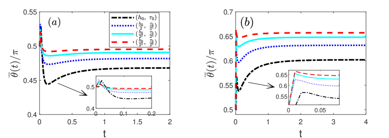
Figure 3: The time history of the average contact angle defined in (62) by using different mesh sizes and time step sizes, where $h_{0}=0.5$ and $\tau_{0}=0.01$. (a) $\theta_{Y}=\pi/2$; (b) $\theta_{Y}=2\pi/3$.

Table 2: Numerical errors between the numerical equilibrium contact angle (at time $t=10$) and the Young’s angle $\theta_{Y}$ for isotropic surface energy, where $h_{0}=0.5$, $\tau_{0}=0.01$.

  $(h,\,\tau)$ $\theta_{Y}=\pi/2$ $\theta_{Y}=2\pi/3$ $|\overline{\theta}-\theta_{Y}|(t=10)$ order $|\overline{\theta}-\theta_{Y}|(t=10)$ order $(h_{0},\,\tau_{0})$ 1.00E-1 - 2.03E-1 - $(\frac{h_{0}}{2},\,\frac{\tau_{0}}{2^{2}})$ 5.70E-2 0.81 1.10E-1 0.88 $(\frac{h_{0}}{2^{2}},\,\frac{\tau_{0}}{2^{4}})$ 2.90E-2 0.97 5.72E-2 0.95 $(\frac{h_{0}}{2^{3}},\,\frac{\tau_{0}}{2^{6}})$ 1.44E-2 1.05 2.98E-2 0.94  

To further assess the accuracy of the numerical method in (24), we define the following average contact angle $\overline{\theta}$

$$\left.\overline{\theta}\right|_{t=t_{m}}:=\frac{1}{N_{{}_{\Gamma}}}\sum_{j=1}^{N_{{}_{\Gamma}}}\arccos\left(\mathbf{c}_{{}_{\Gamma,j}}^{m}\cdot\mathbf{n}_{{}_{\Gamma,j}}^{m}\right),$$ (62)

where $\mathbf{c}_{{}_{\Gamma},_{j}}^{m}$ and $\mathbf{n}_{{}_{\Gamma},_{j}}^{m}$ are numerical approximations of $\mathbf{c}_{{}_{\Gamma}}$ and $\mathbf{n}_{{}_{\Gamma}}$ at $j$th line segment of $\Gamma^{m}$, respectively. The time history of the average contact angles computed using different mesh sizes and time step sizes for $\theta_{Y}=\pi/2$ and $\theta_{Y}=2\pi/3$ are presented in Fig. 3. We observe the convergence of the dynamic contact angle as the mesh is refined. A more quantitative assessment for the average contact angel $\overline{\theta}$ is provided in Table. 2, where we show the error between $\overline{\theta}$ for the equilibrium state ($t=10$) and the Young’s angle $\theta_{Y}$. We observe the error decreases as mesh is refined, and the convergence rate for $|\overline{\theta}-\theta_{Y}|$ is about 1.

5.2 Applications

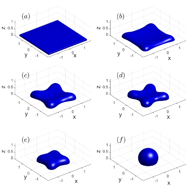
Figure 4: Several snapshots in the evolution of an initially square island film towards its equilibrium shape under the isotropic surface energy: (a) $t=0$; (b) $t=0.004$; (c) $t=0.008$; (d) $t=0.012$; (e) $t=0.020$; (f) $t=0.080$. The initial shape is chosen as a (3.2, 3.2, 0.1) cuboid, and $\theta_{Y}=2\pi/3$.

We present several numerical examples to demonstrate the anisotropic effects on the morphological evolution of thin films in SSD.

Example 1. In this example, we consider the evolution of square island films under: (1) isotropic surface energy $\gamma(\mathbf{n})=1$; (2) ellipsoidal surface energy in (40) with $a_{1}=2,a_{2}=1,a_{3}=1$; and (3) “cusped” surface energy in (41) with $\delta=0.1$. The initial film is chosen as a $(3.2,3.2,0.1)$ cuboid island. The interface is partitioned into $N=18432$ triangles with $K=9345$ vertices, and we take $\tau=1\times 10^{-4}$, $\theta_{Y}=2\pi/3$.

Several snapshots of the morphological evolutions for the thin film under the three anisotropies are shown in Fig. 4, 5 and 6, respectively. In the isotropic case, we observe the four corners of the square island retract much more slowly than that of the four edges at the beginning, thus forming a cross-shaped geometry. As time evolves, the island finally forms a perfectly spherical shape as equilibrium. For ellipsoidal surface energy, the square island forms a grooved shape and then reach an ellipsoidal shape as equilibrium. In the case of “cusped” surface energy, the island maintains a self-similar cuboid shape by gradually decreasing its length, width and increasing its height until reaching the equilibrium state.

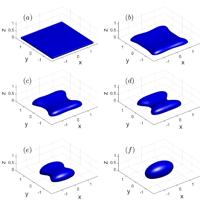
Figure 5: Several snapshots in the evolution of an initially square island film towards its equilibrium shape under the ellipsoidal surface energy: (a) $t=0$; (b) $t=0.004$; (c) $t=0.008$; (d) $t=0.012$; (e) $t=0.020$; (f) $t=0.080$. The initial shape is chosen as a (3.2, 3.2, 0.1) cuboid, and $\theta_{Y}=2\pi/3$. The surface energy is chosen in (40) with $a_{1}=2,a_{2}=1,a_{3}=1$.

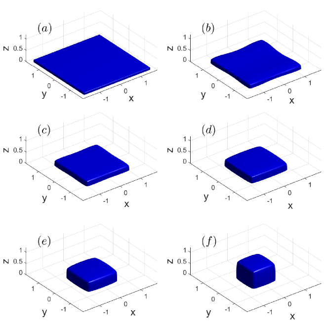
Figure 6: Several snapshots in the evolution of an initially square island film towards its equilibrium shape under the “cusped” surface energy: (a) $t=0$; (b) $t=0.004$; (c) $t=0.008$; (d) $t=0.012$; (e) $t=0.020$; (f) $t=0.080$, where the initial shape is chosen as a (3.2, 3.2, 0.1) cuboid, and $\theta_{Y}=2\pi/3$. The surface energy is chosen in (41) with $\delta=0.1$.

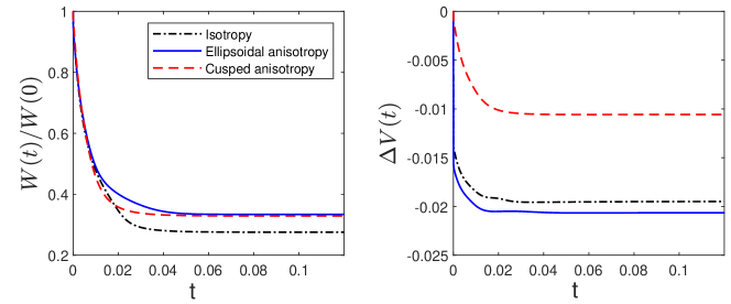
Figure 7: The temporal evolution of the normalized energy $W(t)/W(0)$ (left panel) and the relative volume loss $\Delta V(t)$ (right panel) by using the isotropic surface energy, the ellipsoidal surface energy and cusped surface energy.

In Fig. 7, we plot the temporal evolution of the normalized energy $W(t)/W(0)$ and the relative volume loss $\Delta V$ defined as

$$\Delta V:=\frac{V^{h}(t)-V^{h}(0)}{|V^{h}(0)|},\qquad t\geq 0,$$ (63)

where $V^{h}(0)$ is the total volume of the initial shape. We observe the total free energy of the discrete system decays in time, and the relative volume loss is about 1% to 2%. We note recently a structure-preserving method that can conserve the enclosed volume exactly for surface diffusion was presented in [46], and the generalization to axisymmetric geometric equations was considered in [47]. In addition, an energy-stable method for anisotropic surface diffusion under general anisotropies has been discussed in [48].

Example 2. We investigate the equilibrium shapes of SSD by using different $\theta_{Y}$ and surface energies. We consider the “cusped” surface energy defined in (41) with four different rotations: (1) $\gamma(\mathbf{n})$ defined in (41) with $\delta=0.1$; (2) $\gamma\left(\mbox{\boldmath{$R$}}_{x}(\pi/4)\,\mathbf{n}\right)$; (3) $\gamma\left(\mbox{\boldmath{$R$}}_{y}(\pi/4)\,\mathbf{n}\right)$; (4) $\gamma\left(\mbox{\boldmath{$R$}}_{z}(\pi/4)\,\mathbf{n}\right)$, where $\mbox{\boldmath{$R$}}_{x}(\pi/4)$, $\mbox{\boldmath{$R$}}_{y}(\pi/4)$ and $\mbox{\boldmath{$R$}}_{z}(\pi/4)$ represent the orthogonal matrix for the rotation by an angle $\pi/4$ about the x,y,z-axis using the right-hand rule, respectively. The initial thin film is chosen as a $(3,3,1)$ cuboid island. The interface is partitioned into $N=5376$ triangles with $K=2737$ vertices, and $\tau=10^{-2}$.

As it can be seen from Fig. 8(a)-(c), $\theta_{Y}$ controls the equilibrium contact angle and thus the equilibrium shape. From Fig. 8(d)-(f), we observe that a rotation of the “cusped” anisotropy will result in a corresponding rotation of the equilibrium shape.

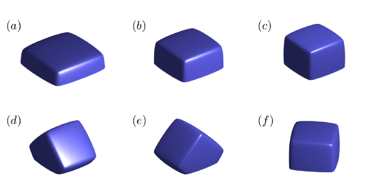
Figure 8: The equilibrium profiles of the island film obtained using different $\theta_{Y}$ and anisotropies. For (a)-(c), we fix $\gamma(\mathbf{n})$ in (41) with $\delta=0.1$, and $\theta_{Y}=\pi/3,~{}\pi/2,~{}2\pi/3$, respectively. For (d) -(f), we set $\theta_{Y}=2\pi/3$ but choose $\gamma\left(\mbox{\boldmath{$R$}}_{x}(\pi/4)\,\mathbf{n}\right)$, $\gamma\left(\mbox{\boldmath{$R$}}_{y}(\pi/4)\,\mathbf{n}\right)$ and $\gamma\left(\mbox{\boldmath{$R$}}_{z}(\pi/4)\,\mathbf{n}\right)$, respectively.

Example 3. We examine the geometric evolution of the square-ring patch under the “cusped” surface energies used in Fig. 8(c)-(f). The initial island is chosen as a $(12,12,1)$ cuboid by cutting out a (10, 10, 1) cuboid from the centre. The interface is partitioned into $N=33792$ triangles with $K=17248$ vertices, and we take $\tau=2\times 10^{-4}$, $\theta_{Y}=2\pi/3$.

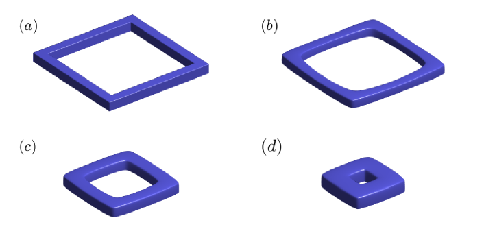
Figure 9: Snapshots of the island film in the evolution of an initially square-ring patch with $\theta_{Y}=2\pi/3$. The surface energy is given by (41) with $\delta=0.1$. (a) $t=0$; (b) $t=1.0$; (c) $t=8.0$; (d) $t=12.6$.

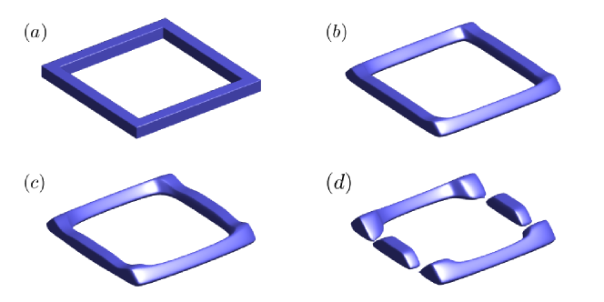
Figure 10: Snapshots of the island film in the evolution of an initially square-ring patch with $\theta_{Y}=2\pi/3$. The surface energy is given by $\gamma(\mbox{\boldmath{$R$}}_{x}(\pi/4)\,\mathbf{n})$, where $\gamma(\mathbf{n})$ is defined in (41) with $\delta=0.1$. (a) $t=0$; (b) $t=0.1$; (c) $t=0.5$; (d) $t=1.12$.

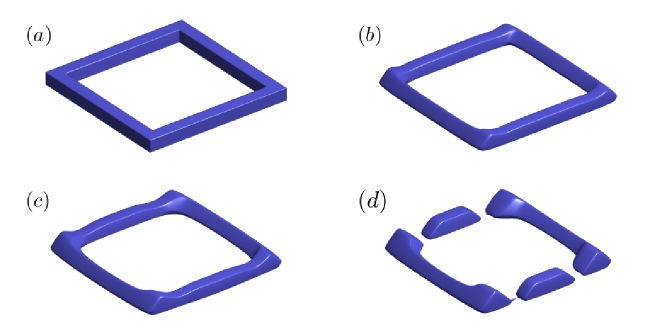
Figure 11: Snapshots of the island film in the evolution of an initially square-ring patch with $\theta_{Y}=2\pi/3$. The surface energy is chosen as $\gamma(\mbox{\boldmath{$R$}}_{y}(\pi/4)\,\mathbf{n})$, where $\gamma(\mathbf{n})$ is defined in (41) with $\delta=0.1$. (a) $t=0$; (b) $t=0.1$; (c) $t=0.5$; (d) $t=1.12$.

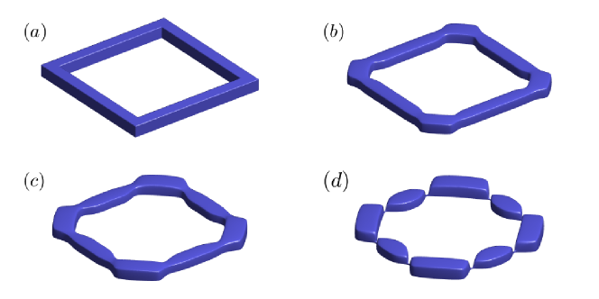
Figure 12: Snapshots of the island film in the evolution of an initially square-ring patch with $\theta_{Y}=2\pi/3$. The surface energy is given by $\gamma(\mbox{\boldmath{$R$}}_{z}(\pi/4)\,\mathbf{n})$, where $\gamma(\mathbf{n})$ is defined in (41) with $\delta=0.1$. (a) $t=0$; (b) $t=0.1$; (c) $t=0.4$; (d) $t=0.76$.

The geometric evolutions for the square-ring island are shown in Fig. 9 -12 for the four cases, respectively. When the surface energy density is given by (41), we observe that the thin square-ring patch gradually shrinks towards the centre to form a self-similar square-ring shape. When the orientation of the anisotropy is rotated with respect to $x$-axis by $\pi/4$, we observe from Fig. 10 that a break-up of the island along the $y$-direction occures. Similarly, a rotation of the anisotropy with respect to $y$-axis results in the breakup of the island along $x$-axis, as expected in Fig. 11. Furthermore, we observe that when the orientation of the anisotropy is rotated with respect to the $z$-axis, the square-ring forms several isolated particles. In these experiments, topological change event could occur when the island is breaking up into small particles. In this situation, we simply show the results before the blowup of the numerical solutions.

It is well-known in isotropic case, the Rayleigh-like instability in the azimuthal direction and the shrinking instability in the radial direction are competing with each other to determine the geometric evolution of a square-ring island [49, 42]. Generally, a very thin square island always breaks up into isolated particles since the Rayleigh-like instability dominates the kinetic evolution; while for a fat square-ring island, the shrinking instability dominates the evolution and makes the island shrink towards the center. Our numerical simulations indicate that anisotropic surface energies play an important role in the evolution of the square-ring island. They can either enhance or mitigate the Rayleigh-like instability in the azimuthal direction, depending on the crystalline alignments.

6 Conclusions

We developed an efficient, accurate, and energy-stable parametric finite element method (ES-PFEM) for solving the sharp-interface model of solid-state dewetting in both the isotropic case and the anisotropic case with anisotropic surface energies in the Riemannian metric form. By reformulating the relaxed contact angle condition as a time-dependent Robin-type of boundary condition for the interface, we obtained a new weak formulation. By using continuous piecewise linear elements in space and the backward Euler method in time, we then discretized the weak formulation to obtain the semi-implicit ES-PFEM. We proved the well-posedness and unconditional energy stability of the numerical method.

We assessed the accuracy and convergence of the proposed ES-PFEM and found that it can attain the second-order convergence rate of the spatial error for the dynamic interface and the first-order convergence rate of the contact angle for the equilibrium interface. Finally, we investigated the anisotropic effects on the evolution of large square islands and square-ring islands by using different anisotropic surface energies. In fact, the proposed ES-PFEM provides a nice tool for simulating different applications in solid-state dewetting in three dimensions.

Appendix A Anisotropic surface gradient

Given a two-dimensional manifold $S$ and a smooth scalar field $f$, the surface gradient of $f$ over $S$ is defined as

$$\nabla_{s}f(\mathbf{X})=\left(\mathbb{I}-\mathbf{n}\otimes\mathbf{n}\right)\nabla f(\mathbf{X}):=(\underline{D}_{1}f(\mathbf{X}),~{}\underline{D}_{2}f(\mathbf{X}),~{}\underline{D}_{3}f(\mathbf{X}))^{T},\quad\mathbf{X}\in S,$$ (64)

where $\mathbb{I}\in\mathbb{R}^{3\times 3}$ is the identity matrix and $\mathbf{n}$ is the unit normal to $S$.

Let $G\in\mathbb{R}^{3\times 3}$ be a symmetric positive definite (SPD) matrix, we follow the notations in [38] and define the anisotropic surface gradient associated with the SPD matrix $\widetilde{G}=({\rm det}{G})^{-\frac{1}{2}}G$ as

$$\nabla_{s}^{\widetilde{G}}f(\mathbf{X})=\sum_{i=1}^{2}(\partial_{\mathbf{t}_{i}}f)(\mathbf{X})\,\mathbf{t}_{i},\qquad\mathbf{X}\in S,$$ (65)

where $\partial_{\mathbf{t}_{i}}f=\mathbf{t}_{i}\cdot(\nabla_{s}\,f)$ is the directional derivative, and $\left\{\mathbf{t}_{1},~{}\mathbf{t}_{2}\right\}$ is the orthogonal basis of the tangential space of $S$ with respect to $\widetilde{G}$ at the point of interest $\mathbf{X}$, i.e.,

$$\mathbf{t}_{i}\cdot(\widetilde{G}\,\mathbf{t}_{j})=\delta_{ij},\quad\mathbf{t}_{i}\cdot\mathbf{n}(\mathbf{X})=0,\qquad i,j=1,2.$$ (66)

Moreover, given a vector-valued smooth function $g$, the anisotropic surface divergence and anisotropic surface gradient are then defined respectively as

$$(\nabla_{s}^{\widetilde{G}}\cdot\mbox{\boldmath{$g$}})(\mathbf{X})=\sum_{i=1}^{2}(\partial_{\mathbf{t}_{i}}\mbox{\boldmath{$g$}})(\mathbf{X})\cdot({\widetilde{G}}\,\mathbf{t}_{i}),$$ (67a)

$$(\nabla_{s}^{\widetilde{G}}\,\mbox{\boldmath{$g$}})(\mathbf{X})=\sum_{i=1}^{2}(\partial_{\mathbf{t}_{i}}\,\mbox{\boldmath{$g$}})(\mathbf{X})\otimes(\widetilde{G}\mathbf{t}_{i}).$$ (67b)

Appendix B Differential calculus

Given the surface energy density $\gamma(\mathbf{n})$ in (39) and the moving surface $S(t)$ with boundary $\Gamma(t)$, then we have the following equation hold (see Lemma 2.1 in [24]):

$$\frac{\mathrm{d}}{\mathrm{d}t}\int_{S(t)}\gamma(\mathbf{n})\,\mathrm{d}A=\int_{S(t)}\mu\,\mathbf{n}\cdot\mbox{\boldmath{$v$}}\,\mathrm{d}A+\int_{\Gamma(t)}\mathbf{c}_{{}_{\Gamma}}^{\gamma}\cdot\mbox{\boldmath{$v$}}\,\mathrm{d}s,$$ (68)

where $\mu$ is the chemical potential defined in (42b) and $v$ is the velocity of $S(t)$.

Besides, we have (see Lemma 3.2 in [39]):

$$\frac{\mathrm{d}}{\mathrm{d}t}\sum_{i=1}^{L}\int_{S(t)}\gamma_{i}(\mathbf{n})\,\mathrm{d}A:=\sum_{i=1}^{L}\int_{S(t)}\gamma_{i}(\mathbf{n})\left(\nabla_{s}^{\widetilde{G}_{i}}\,\mathbf{X},~{}\nabla_{s}^{\widetilde{G}_{i}}\mbox{\boldmath{$v$}}\right)_{\widetilde{G}_{i}}\,\mathrm{d}A,$$ (69)

where we define the inner product with respect to a particular matrix $\widetilde{G}$ for $\mathbf{u},~{}\mathbf{v}$ via

$$\Bigl{(}\nabla_{s}^{\widetilde{G}}\mathbf{u},~{}\nabla_{s}^{\widetilde{G}}\mathbf{v}\Bigr{)}_{\widetilde{G}}=\sum_{i=1}^{2}\Bigl{(}\partial_{\mathbf{t}_{i}}\mathbf{u},~{}\partial_{\mathbf{t}_{i}}\mathbf{v}\Bigr{)}_{\widetilde{G}}=\sum_{i=1}^{2}\partial_{\mathbf{t}_{i}}\mathbf{u}\cdot(\widetilde{G}\,\partial_{\mathbf{t}_{i}}\mathbf{v}),$$ (70)

with $\{\mathbf{t}_{1},~{}\mathbf{t}_{2}\}$ satisfying (66). In particular, when $L=1$ and $\widetilde{G}_{1}=G_{1}=\mathbb{I}$, Eq. (69) will reduce to the Reynolds transport theorem on $S(t)$

$$\frac{\mathrm{d}}{\mathrm{d}t}\left|S(t)\right|=\int_{S(t)}\nabla_{s}\mathbf{X}:\nabla_{s}\mbox{\boldmath{$v$}}\,\mathrm{d}A.$$ (71)

Combining (68) and (69) yields

$$\int_{S(t)}\mu\,\mathbf{n}\cdot\mbox{\boldmath{$v$}}\,\mathrm{d}A-\sum_{i=1}^{L}\int_{S(t)}\gamma_{i}(\mathbf{n})\,\left(\nabla_{s}^{\widetilde{G}_{i}}\,\mathbf{X},~{}\nabla_{s}^{\widetilde{G}_{i}}\mbox{\boldmath{$v$}}\right)_{\widetilde{G}_{i}}\,\mathrm{d}A+\int_{\Gamma(t)}\mathbf{c}_{{}_{\Gamma}}^{\gamma}\cdot\mbox{\boldmath{$v$}}\,\mathrm{d}s=0.$$ (72)

When $L=1$ and $\widetilde{G}_{1}=G_{1}=\mathbb{I}$, Eq. (72) will reduce to

$$\int_{S(t)}\mathcal{H}\,\mathbf{n}\cdot\mbox{\boldmath{$v$}}\,\mathrm{d}A-\int_{S(t)}\nabla_{s}\mathbf{X}:\nabla_{s}\mbox{\boldmath{$v$}}\,\mathrm{d}A+\int_{\Gamma(t)}\mathbf{c}_{{}_{\Gamma}}\cdot\mbox{\boldmath{$v$}}\,\mathrm{d}s=0.$$ (73)

Appendix C Relevant inequalities

Given the surface energy density $\gamma(\mathbf{n})$ in (39), and the polygonal surface $S^{m}:=\mathbf{X}^{m}(\cdot)\in\mathbb{X}^{m}$ in (19), where $\mathbb{X}^{m}$ is defined in (20). For $\mathbf{Y}\in\mathbb{X}^{m}$, we have (see Lemma 3.1 in [38]):

$$\frac{1}{2}\int_{\sigma_{j}^{m}}\gamma_{i}(\mathbf{n}^{m})\left(\nabla_{s}^{\widetilde{G}_{i}}\,\mathbf{Y},~{}\nabla_{s}^{\widetilde{G}_{i}}\mathbf{Y}\right)_{\widetilde{G}_{i}}\,\mathrm{d}A\geq\int_{\mathbf{Y}(\sigma_{j}^{m})}\gamma_{i}(\mathbf{n}(\mathbf{Y}))\,\mathrm{d}A,\quad 1\leq i\leq L,\quad 1\leq j\leq N,$$ (74)

and the equality holds when $\mathbf{Y}=\mathbf{X}^{m}$. When $\gamma_{i}\equiv 1$, i.e, $G_{i}=\widetilde{G}_{i}=\mathbb{I}$, we obtain for $1\leq j\leq N$

$$\frac{1}{2}\int_{\sigma_{j}^{m}}\nabla_{s}\mathbf{Y}:\nabla_{s}\mathbf{Y}\,\mathrm{d}A\geq\int_{\mathbf{Y}(\sigma_{j}^{m})}\,\mathrm{d}A=|\mathbf{Y}(\sigma_{j}^{m})|,$$ (75a)

$$\frac{1}{2}\int_{\sigma_{j}^{m}}\nabla_{s}\mathbf{X}^{m}:\nabla_{s}\mathbf{X}^{m}\,\mathrm{d}A=\int_{\sigma_{j}^{m}}\,\mathrm{d}A=|\sigma_{j}^{m}|.$$ (75b)

Acknowledgements. The work of Bao was supported by Singapore MOE grant MOE2019-T2-1-063 (R-146-000-296-112). The work of Zhao was supported by the Singapore MOE grant R-146-000-285-114.

References

- [1] C. V. Thompson, Solid-state dewetting of thin films, Annu. Rev. Mater. Res. 42 (2012) 399–434.
- [2] J. Mizsei, Activating technology of SnO2 layers by metal particles from ultrathin metal films, Sensor Actuat B-Chem. 16 (1) (1993) 328–333.
- [3] S. Rath, M. Heilig, H. Port, J. Wrachtrup, Periodic organic nanodot patterns for optical memory, Nano Lett. 7 (12) (2007) 3845–3848.
- [4] S. Randolph, J. Fowlkes, A. Melechko, K. Klein, H. Meyer III, M. Simpson, P. Rack, Controlling thin film structure for the dewetting of catalyst nanoparticle arrays for subsequent carbon nanofiber growth, Nanotechnology 18 (46) (2007) 465304.
- [5] J. Ye, C. V. Thompson, Mechanisms of complex morphological evolution during solid-state dewetting of single-crystal nickel thin films, Appl. Phys. Lett. 97 (7) (2010) 071904.
- [6] J. Ye, C. V. Thompson, Anisotropic edge retraction and hole growth during solid-state dewetting of single crystal nickel thin films, Acta Mater. 59 (2) (2011) 582–589.
- [7] D. Amram, L. Klinger, E. Rabkin, Anisotropic hole growth during solid-state dewetting of single-crystal Au–Fe thin films, Acta Mater. 60 (6-7) (2012) 3047–3056.
- [8] E. Rabkin, D. Amram, E. Alster, Solid state dewetting and stress relaxation in a thin single crystalline Ni film on sapphire, Acta Mater. 74 (2014) 30–38.
- [9] A. Herz, A. Franz, F. Theska, M. Hentschel, T. Kups, D. Wang, P. Schaaf, Solid-state dewetting of single-and bilayer Au-W thin films: Unraveling the role of individual layer thickness, stacking sequence and oxidation on morphology evolution, AIP Adv. 6 (3) (2016) 035109.
- [10] M. Naffouti, T. David, A. Benkouider, L. Favre, A. Delobbe, A. Ronda, I. Berbezier, M. Abbarchi, Templated solid-state dewetting of thin silicon films, Small 12 (44) (2016) 6115–6123.
- [11] O. Kovalenko, S. Szabó, L. Klinger, E. Rabkin, Solid state dewetting of polycrystalline Mo film on sapphire, Acta Mater. 139 (2017) 51–61.
- [12] W. Jiang, W. Bao, C. V. Thompson, D. J. Srolovitz, Phase field approach for simulating solid-state dewetting problems, Acta Mater. 60 (15) (2012) 5578–5592.
- [13] D. J. Srolovitz, S. A. Safran, Capillary instabilities in thin films: I. Energetics, J. Appl. Phys. 60 (1) (1986) 247–254.
- [14] Y. Wang, W. Jiang, W. Bao, D. J. Srolovitz, Sharp interface model for solid-state dewetting problems with weakly anisotropic surface energies, Phys. Rev. B 91 (2015) 045303.
- [15] W. Jiang, Y. Wang, Q. Zhao, D. J. Srolovitz, W. Bao, Solid-state dewetting and island morphologies in strongly anisotropic materials, Scr. Mater. 115 (2016) 123–127.
- [16] W. Bao, W. Jiang, Y. Wang, Q. Zhao, A parametric finite element method for solid-state dewetting problems with anisotropic surface energies, J. Comput. Phys. 330 (2017) 380–400.
- [17] W. Bao, W. Jiang, D. J. Srolovitz, Y. Wang, Stable equilibria of anisotropic particles on substrates: a generalized Winterbottom construction, SIAM J. Appl. Math. 77 (6) (2017) 2093–2118.
- [18] E. Dornel, J. Barbe, F. De Crécy, G. Lacolle, J. Eymery, Surface diffusion dewetting of thin solid films: Numerical method and application to Si/SiO2, Phys. Rev. B 73 (11) (2006) 115427.
- [19] H. Wong, P. Voorhees, M. Miksis, S. Davis, Periodic mass shedding of a retracting solid film step, Acta Mater. 48 (8) (2000) 1719–1728.
- [20] G. H. Kim, R. V. Zucker, J. Ye, W. C. Carter, C. V. Thompson, Quantitative analysis of anisotropic edge retraction by solid-state dewetting of thin single crystal films, J. Appl. Phys. 113 (4) (2013) 043512.
- [21] W. Kan, H. Wong, Fingering instability of a retracting solid film edge, J. Appl. Phys. 97 (4) (2005) 043515.
- [22] W. W. Mullins, Theory of thermal grooving, J. Appl. Phys. 28 (3) (1957) 333–339.
- [23] D. J. Srolovitz, S. A. Safran, Capillary instabilities in thin films: II. Kinetics, J. Appl. Phys. 60 (1) (1986) 255–260.
- [24] W. Jiang, Q. Zhao, W. Bao, Sharp-interface model for simulating solid-state dewetting in three dimensions, SIAM J. Appl. Math. 80 (4) (2020) 1654–1677.
- [25] M. Dziwnik, A. Münch, B. Wagner, An anisotropic phase-field model for solid-state dewetting and its sharp-interface limit, Nonlinearity 30 (2017) 1465–1496.
- [26] M. Naffouti, R. Backofen, M. Salvalaglio, T. Bottein, M. Lodari, A. Voigt, T. David, A. Benkouider, I. Fraj, L. Favre, et al., Complex dewetting scenarios of ultrathin silicon films for large-scale nanoarchitectures, Sci. Adv. 3 (11) (2017) eaao1472.
- [27] Q.-A. Huang, W. Jiang, J. Z. Yang, An efficient and unconditionally energy stable scheme for simulating solid-state dewetting of thin films with isotropic surface energy, Commu. Comput. Phys. 26 (2019) 1444–1470.
- [28] W. C. Carter, A. R. Roosen, J. W. Cahn, J. E. Taylor, Shape evolution by surface diffusion and surface attachment limited kinetics on completely faceted surfaces, Acta Metall. Mater. 43 (12) (1995) 4309–4323.
- [29] R. V. Zucker, G. H. Kim, W. C. Carter, C. V. Thompson, A model for solid-state dewetting of a fully-faceted thin film, C. R. Physique 14 (7) (2013) 564–577.
- [30] O. Pierre-Louis, A. Chame, Y. Saito, Dewetting of ultrathin solid films, Phys. Rev. Lett. 103 (19) (2009) 195501.
- [31] P. Du, M. Khenner, H. Wong, A tangent-plane marker-particle method for the computation of three-dimensional solid surfaces evolving by surface diffusion on a substrate, J. Comput. Phys. 229 (3) (2010) 813–827.
- [32] U. F. Mayer, Numerical solutions for the surface diffusion flow in three space dimensions, Comput. Appl. Math. 20 (3) (2001) 361–379.
- [33] E. Bänsch, P. Morin, R. H. Nochetto, A finite element method for surface diffusion: the parametric case, J. Comput. Phys. 203 (1) (2005) 321–343.
- [34] F. Hausser, A. Voigt, A discrete scheme for parametric anisotropic surface diffusion, J. Sci. Comput. 30 (2) (2007) 223–235.
- [35] P. Pozzi, Anisotropic mean curvature flow for two-dimensional surfaces in higher codimension: a numerical scheme, Interface Free Bound. 10 (4) (2008) 539–576.
- [36] J. W. Barrett, H. Garcke, R. Nürnberg, On the parametric finite element approximation of evolving hypersurfaces in , J. Comput. Phys. 227 (9) (2008) 4281–4307.
- [37] J. W. Barrett, H. Garcke, R. Nürnberg, Parametric finite element approximations of curvature driven interface evolutions, Handb. Numer. Anal. (Andrea Bonito and Ricardo H. Nochetto, eds.) 21 (2020) 275–423.
- [38] J. W. Barrett, H. Garcke, R. Nürnberg, A variational formulation of anisotropic geometric evolution equations in higher dimensions, Numer. Math. 109 (1) (2008) 1–44.
- [39] J. W. Barrett, H. Garcke, R. Nürnberg, Parametric approximation of surface clusters driven by isotropic and anisotropic surface energies, Interface Free Bound. 12 (2) (2010) 187–234.
- [40] J. W. Barrett, H. Garcke, R. Nürnberg, Finite-element approximation of coupled surface and grain boundary motion with applications to thermal grooving and sintering, Eur. J. Appl. Math. 21 (6) (2010) 519–556.
- [41] W. Jiang, Q. Zhao, Sharp-interface approach for simulating solid-state dewetting in two dimensions: a Cahn-Hoffman -vector formulation, Physica D 390 (2019) 69–83.
- [42] Q. Zhao, W. Jiang, W. Bao, A parametric finite element method for solid-state dewetting problems in three dimensions, SIAM J. Sci. Comput. 42 (1) (2020) B327–B352.
- [43] Q. Zhao, W. Jiang, W. Bao, An energy-stable parametric finite element method for simulating solid-state dewetting, IMA J. Numer. Anal. 41 (2021) 2026–2055.
- [44] D. W. Hoffman, J. W. Cahn, A vector thermodynamics for anisotropic surfaces: I. Fundamentals and application to plane surface junctions, Surface Science 31 (1972) 368–388.
- [45] J. W. Cahn, D. W. Hoffman, A vector thermodynamics for anisotropic surfaces: II. Curved and faceted surfaces, Acta Metall. 22 (10) (1974) 1205–1214.
- [46] W. Bao, Q. Zhao, A structure-preserving parametric finite element method for surface diffusion, SIAM J. Numer. Anal. 59 (5) (2021) 2775–2799.
- [47] W. Bao, H. Garcke, R. Nürnberg, Q. Zhao, Volume-preserving parametric finite element methods for axisymmetric geometric evolution equations, J. Comput. Phys. 460 (2022) 111180.
- [48] Y. Li, W. Bao, An energy-stable parametric finite element method for anisotropic surface diffusion, J. Comput. Phys. 446 (2021) 110658.
- [49] W. Jiang, Q. Zhao, T. Qian, D. J. Srolovitz, W. Bao, Application of Onsager’s variational principle to the dynamics of a solid toroidal island on a substrate, Acta Mater. 163 (2019) 154–160.