Unifying Homophily and Heterophily Network Transformation via Motifs

Abstract

Higher-order proximity (HOP) is fundamental for most network embedding methods due to its significant effects on the quality of node embedding and performance on downstream network analysis tasks. Most existing HOP definitions are based on either homophily to place close and highly interconnected nodes tightly in embedding space or heterophily to place distant but structurally similar nodes together after embedding. In real-world networks, both can co-exist, and thus considering only one could limit the prediction performance and interpretability. However, there is no general and universal solution that takes both into consideration. In this paper, we propose such a simple yet powerful framework called homophily and heterophliy preserving network transformation (H²NT) to capture HOP that flexibly unifies homophily and heterophily. Specifically, H²NT utilises motif representations to transform a network into a new network with a hybrid assumption via micro-level and macro-level walk paths. H²NT can be used as an enhancer to be integrated with any existing network embedding methods without requiring any changes to latter methods. Because H²NT can sparsify networks with motif structures, it can also improve the computational efficiency of existing network embedding methods when integrated. We conduct experiments on node classification, structural role classification and motif prediction to show the superior prediction performance and computational efficiency over state-of-the-art methods. In particular, DeepWalk-based H²NT achieves 24% improvement in terms of precision on motif prediction, while reducing 46% computational time compared to the original DeepWalk.

1 Introduction

Networks are ubiquitous in the real world, such as social networks Fortunato (2010), biological networks Girvan and Newman (2002) and traffic networks Asif et al. (2016). Network embedding (a.k.a. graph embedding) learns low-dimensional latent representations of nodes while preserving the structure and inherent properties of the network. It has been successfully applied in node classification Kipf and Welling (2017), link prediction Zhang et al. (2018b), and community detection Wang et al. (2017).

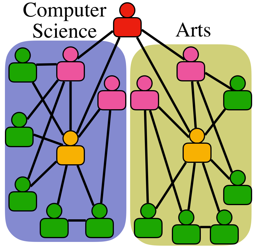
(a) Homophily

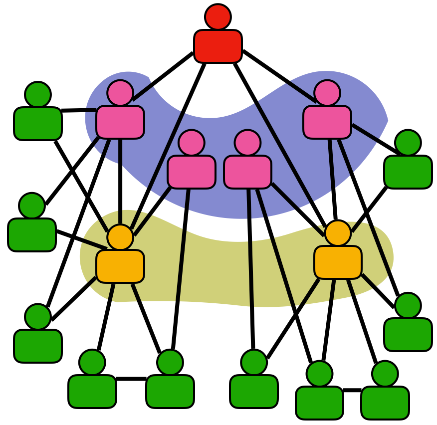
(b) Heterophily

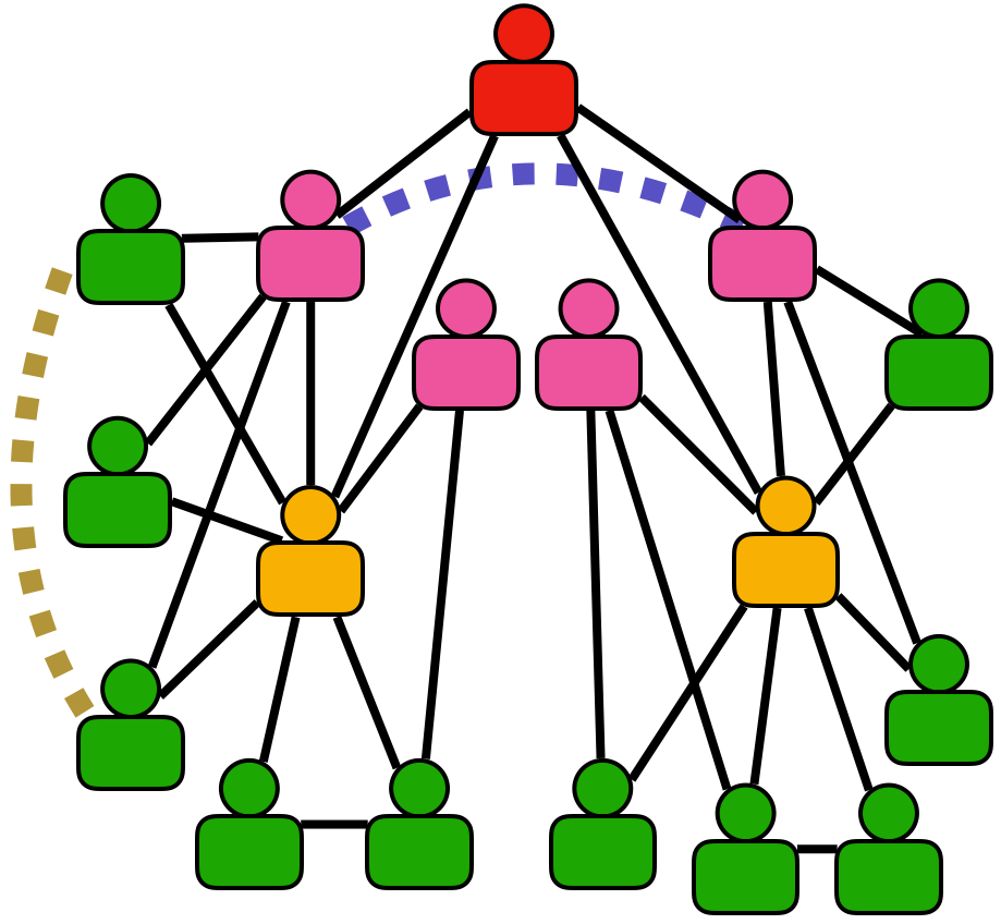
(c) Hybrid (proposed)

Figure 1: Three categories of higher-order proximity assumptions for network embedding: homophily, heterophily and hybrid (proposed).

Preserving higher-order proximity (HOP) instead of only considering direct neighbourhood relationship (e.g., adjacency matrix) has been shown to be effective for network embedding since it can capture rich underlying structures of networks Cao et al. (2015); Tang et al. (2015); Zhang et al. (2018b). Based on the proximity assumption, there are three categories of HOP: homophily, heterophily, and hybrid. In homophily Fortunato (2010), nodes that are highly interconnected and in the same community should be placed tightly in embedding space. For example, in Fig. 1(a), proximity within the same department should be higher than different ones after embedding, which benefits community detection Wang et al. (2016) and node classification Perozzi et al. (2014). For heterophily Klicpera et al. (2019), nodes that are far away and in different groups, but due to their strong structural similarity, they should be close after embedding. For example, in Fig. 1(b), department heads from different academic areas (yellow nodes) should have stronger relation than their immediate neighbours due to the same job role under heterophily, good for structural role classification Rossi et al. (2019). For hybrid assumption, both homophily and heterophily can be flexibly preserved, which potentially benefits (long/short-range) link prediction task (e.g., Fig. 1(c)).

To preserve HOP under the homophily assumption, DeepWalk Perozzi et al. (2014) employs random walks to generate node sequences analogous to word sentences, and then the HOP is approximately captured by a Skip-gram model Mikolov et al. (2013). Graph convolutional network (GCN) Kipf and Welling (2017) aggregates the features of local neighbours for central node representation so that feature vectors of nodes within the same community are more similar than those in different communities. Arbitrary-order proximity embedding (AROPE) Zhang et al. (2018b) effectively and accurately preserves arbitrary-order proximity by reweighting the eigen-decompostion. To preserve HOP under the heterophily assumption, struc2vec Ribeiro et al. (2017) first encodes the node structural similarity into a multi-layer graph, and then DeepWalk is performed on this multi-layer graph to learn node representations. A recent transformation model graph diffusion convolution (GDC) Klicpera et al. (2019) generates a new network by constructing a diffusion graph obtained by a polynomial function, and then sparsify this diffusion graph by setting a threshold, but still overlooks the heterophily assumption.

The higher-order proximities in the aforementioned methods are defined to be either homophily or heterophily. Such “one-size-fit-all” proximity representation potentially limits the performance and interpretation on many network-based tasks. To alleviate this problem, one representative hybrid solution is the node2vec method Grover and Leskovec (2016), which flexibly adopts both breadth-first and depth-first search strategies to conduct a biased random-walk process. However, it is designed specifically for random-walk-based methods and cannot take advantage of other more powerful network embedding methods proposed recently, such as GCN and AROPE. Additionally, most existing proximity preserving methods still rely on simple pairwise relations without considering motifs (e.g., triangles, $4$-vertex cliques) that can directly capture interactions between more than two nodes Benson et al. (2016). For example, triangular structures, with three reciprocated edges connecting three nodes, play important roles in social networks Kossinets and Watts (2006) that can be partitioned into dense triangle communities with motif spectral clustering (MotifSC) Benson et al. (2016). This paper will focus on fundamental triangle motif structure, though our proposed method can be easily extended to other motifs.

Table 1: Comparison with state-of-the-art methods in term of fulfilled (✔) and missing (✘) properties.

Property	DeepWalk	LINE	node2vec	AROPE	GCN	struc2vec	MotifSC	H2NT
Homophily	✔	✔	✔	✔	✔	✘	✔	✔
Heterophily	✘	✘	✔	✘	✘	✔	✘	✔
Motif	✘	✘	✘	✘	✘	✘	✔	✔

To design a general framework with a hybrid HOP assumption, we propose a homophily and heterophliy preserving network transformation (H²NT) with motif representations. Our H²NT defines a new HOP by micro-level and macro-level walk paths as two complementary components to represent homophily and heterophily. The micro-level walk paths embody the homophily assumption, aiming to collect the similarity of close neighbours according to their homophily levels generated by motif information. The macro-level walk paths embody the heterophily assumption, aiming to encourage walk paths to explore global information according to structural similarity.

As a general framework, H²NT is not limited to one specific algorithm but can be integrated to any network embedding algorithm as a preprocessing step, without requiring changing their cores. Furthermore, the two walk path strategies can only rely on local motif structures and sparsify networks and subsequently improve the computational efficiency when we integrate H²NT with existing network embedding algorithms. Table 1 compares three desirable properties to show the uniqueness of H²NT compared with several state-of-the-art (SOTA) methods. To summarise, the contributions of our paper are as follows:

1. We propose micro-level and macro-level walk paths to preserve homophily and heterophily in HOP by theoretically studying why most HOP preserving embedding methods only hold a homophily assumption.

2. We propose a simple and novel framework to unify homophily and heterophily representations according to micro-level and macro-level walk paths, and three instantiations.

3. We conduct experiments on three tasks, node classification, structural role classification, and motif prediction (a generalised link prediction problem) to show the superior performance over SOTA methods.

2 Preliminary

2.1 Notations.

We denote scalars by lowercase letters, e.g., $d$, vectors by lowercase boldface letters, e.g., $\mathbf{d}$, matrices by uppercase boldface, e.g., $\mathbf{D}$. Let $G=(V,E)$ be an undirected unweighted graph (network) with $V$ = {v₁, v₂, …, v_n} being the set of $n$ nodes, i.e., $n$ = $|V|$, and $E$ = {e₁, e₂, …, e_n} being the set of edges connecting two nodes.

2.2 Higher-Order Proximity.

Network embedding aims to learn latent, low-dimensional representation of nodes while preserving network topology Zhang et al. (2018a). Prior works have demonstrated that, the higher-order proximities between nodes are of tremendous importance in capturing the underlying structure of the network Cao et al. (2015); Ou et al. (2016); Yang et al. (2017); Feng et al. (2018). The adjacency matrix $\mathbf{A}$ can be treated as the first-order proximity, which captures the pairwise proximity between nodes. However, the first-order proximity is very sparse and insufficient to fully model the relationships between nodes in most cases. In order to characterise the connections between nodes better, HOP is widely studied. Given $\mathbf{A}$, an HOP can be defined as a polynomial function of $\mathbf{A}$ Zhang et al. (2018b): $\mathbf{S}=w_{1}\mathbf{A}+w_{2}\mathbf{A}^{2}+\ldots+w_{l}\mathbf{A}^{l},$ where $l$ is the order, and $w_{1},...,w_{l}$ are the weights for each term. Matrix $\mathbf{A}^{l}$ denotes the $l$th-order proximity matrix, with multiplication of $l$ matrices $\mathbf{A}$. The $l$th-order proximity value between nodes $v_{i}$ and $v_{j}$ is denoted as $a_{ij}^{(l)}$.

3 Methodology

3.1 Theoretical Framework and Motivations

In this section, we theoretically reveal why most network embedding algorithms only hold a homophily assumption in HOP. This motivates us to propose micro-level and macro-level walk paths strategies to represent homophily and heterophily in HOP.

We first introduce a fully-connected planted partition model (PPM) as follows Condon and Karp (2001):

Definition 1.

(Fully-Connected PPM)  Let $G_{f}\sim G_{f}(mr,r,p,q)$ be a graph sampled from the planted partition model on $mr$ vertices, with $r$ clusters $C=\{C_{1},\cdots,C_{i},\cdots,C_{r}\}$ each with exactly $m$ vertices. The edge set is then generated as follows: two vertices $\{v_{i},v_{j}\}\in C_{i}$ are connected with weight $p$ otherwise with weight $q<p$ to ensure well-connected clusters.

We prove the following lemma to show a relationship between homophily and HOP.

Lemma 1.

Let $G_{f}\sim G_{f}(mr,r,p,q)$ be a fully-connected PPM with $r$ clusters $C=\{C_{1},\cdots,C_{i},\cdots,C_{r}\}$, nodes { $v_{i},v_{j}\}\in C_{s}$ and $v_{k}\in C_{t}$, the value of $l^{th}$-order proximity between $v_{i}$ and $v_{j}$ is $a_{ij}^{(l)}$, then $a_{ik}^{(l)}<a_{ij}^{(l)}.$

Our proof as shown in Supplementary Material is based on the following rule.

Rule 1.

(Chapman-Kolmogorov equations) Tijms (2012),

$$a_{ik}^{(l)}=\sum_{z=1}^{kn}a_{iz}^{(l-1)}\cdot a_{zk},\ \ a_{ij}^{(l)}=\sum_{z=1}^{kn}a_{iz}^{(l-1)}\cdot a_{zj}.$$ (1)

Observations. We have two main observations: 1) From Lemma 1, we see that most existing HOPs hold the assumption of homophily, so that in the embedding space, distance of two nodes residing in different communities being inherently larger than that of those in the same community. 2) Eqs (1) reveal that HOP between any pair of nodes $v_{i}$ and $v_{j}$ essentially represents the total similarity of a sequence of nodes traversed by all possible walk paths from $v_{i}$ to $v_{j}$, and all walk paths share the same contributions to represent $a_{ij}^{(l)}$ regardless of various downstream network tasks. However, we argue that every walk path should have task-relevant contributions to $a_{ij}^{(l)}$. This inspires the following question: are there some specific walk paths that characterise the task-relevant HOP w.r.t. homophily or heterophily? Subsequently, to explicitly reveal the characteristics of HOP, we categorise all possible walk paths into micro-level and macro-level walk paths as two complementary components to represent HOP. Our proposed definitions are below.

Definition 2.

(Micro-level walk path) A micro-level walk path connecting $v_{i}$ and $v_{j}$ is a sequence of vertices $V^{\prime}=($$v_{i}$, $v_{k}$,$\cdots$, $v_{j}$) traversed a sequence of edges $E^{\prime}=($$e_{1}$, $e_{1}$,$\cdots$, $e_{n}$) that ensures $V^{\prime}\subseteq C_{i}$ and $E^{\prime}\subseteq C_{i}$.

Definition 3.

(Macro-level walk path) A macro-level walk path connecting $v_{i}$ and $v_{j}$ is a sequence of vertices $V^{\prime}=($$v_{i}$, $v_{k}$,$\cdots$, $v_{j}$) traversed a sequence of edges $E^{\prime}=($$e_{1}$, $e_{1}$,$\cdots$, $e_{n}$) and $E^{\prime}\cap C_{j}\neq\phi$ and $E^{\prime}\cap C_{i}\neq\phi$ and $i\neq j$.

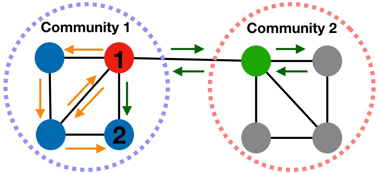
Figure 2: Illustration: 1) Micro-level (orange arrows within the community 1) and macro-level (dark green arrows across communities 1 and 2) walk paths represent the 5th-order proximity between nodes 1 and 2; 2) The green node contributes more centrality to the red node than any blue node.

For example, in Fig 2, we observe that orange (micro-level) path and dark-green (macro-level) path play very different roles to induce a five-step connectivity pattern from node 1 to node 2, although both can contribute to 5th-order proximity between node 1 and 2. Under the homophily assumption, the orange path has more expressive power than the dark-green path since it is likely to leverage tightly close neighbourhood similarity within a community, which may benefit community detection and node classification tasks. In contrast, under the heterophily assumption, the dark-green path has more appropriate expressive power than the orange path to heterophily since it tends to use weak-connectivity and distant neighbourhood similarity across communities, good for structural role classification. Moreover, only homophily or heterophily cannot be suitable for all network-based tasks.

In general, micro/macro-level walk paths allow us to capture the structure of the traversed region and provide an attention mechanism to guide the walk. This allows us to focus on task-relevant parts of the graph while eliminating the noise in the rest of the graph which results in the network embedding that provides better predictive performance. Note that different from the breadth-first and depth-first approximately search in node2vec, fixed length of micro-level and macro-level walk paths will be exhaustedly and accurately considered to represent HOP between two nodes. While they share a general idea that representation of a node is determined by its neighbourhoods that need to be flexibly defined.

Building on the above discussions, in the following we propose H²NT that defines new HOP to flexibly preserve both homophily and heterophily by characterising walk paths with micro-level and macro-level walk paths. It is a generic model that can be used as a preprocessing step to provide input to any network embedding methods.

3.2 Homophily Proximity Representation

To represent homophily proximity, adjacency matrix $\mathbf{A}$ or random walk matrix $\mathbf{P}$ is widely used but both are noisy and sparse. Another choice is to perform community detection so that homophily character of each edge can be clearly shown, such as by spectral clustering Ng et al. (2002)). However, this will lead to a binary-valued output edge (i.e., within or across communities) and limits our ability in exploring unseen patterns of a network.

To address the above challenges, we adopt a scalable and smooth community detection method with motif representations Benson et al. (2016) to represent homophily proximity as $\mathbf{A}_{M}$,

$$\mathbf{A}_{M}(i,j)=\sum_{v_{i},v_{j}\in\mathcal{V}}\underline{1}\left(v_{i},v_{j}\operatorname{occurin}M\right)$$ (2)

where $i\neq j$, $v_{i}$ and $v_{j}$ belong to motif $M$ , and 1($s$) is the truth-value indicator function, i.e., 1($s$) = 1 if the statement s is true and 0 otherwise. Note that the weight is added to $\mathbf{A}_{M}(i,j)$ only if node $v_{i}$ and $v_{j}$ occur in the given motif $M$. In this paper, we only focus on undirected triangle motif, but it can be easily generated to any other type of motifs. The intuition of homophily proximity representation (Eq. (2)) is that motif representation smooths out the neighbourhood over the graph, acting as denoise filter due to removed edges that do not participate in any motif. More importantly, the value in homophily proximity representation indicates the level of homophily as quantified in Lemma 2 extended from Tsourakakis et al. (2017) and our proof as shown in Supplementary Material:

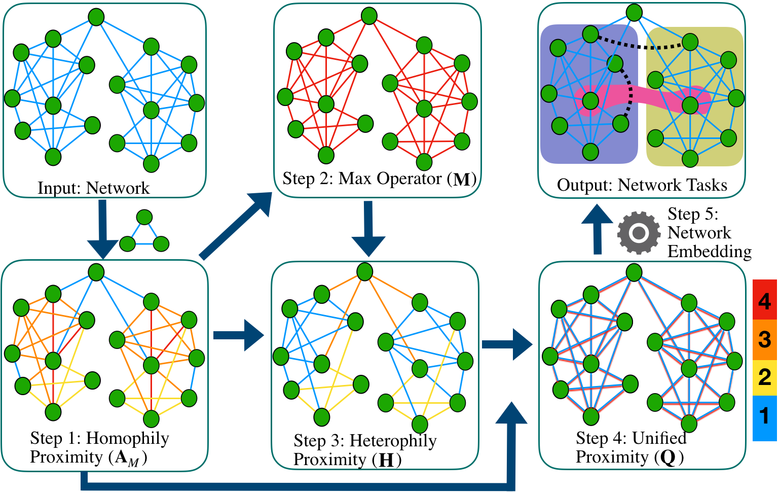
Figure 3: The H²NT framework. The colour bar indicates the weight scales of edges. (See text for details.)

Lemma 2.

Let $G\sim G(mk,k,p,q)$ be an unweitghted graph sampled by a generalized PPM, $\{v_{i},v_{j}\}\in C_{i}$ and $\{v_{k}\}\in C_{j}$, $\{v_{d}\}\in C_{b}$, $j\neq b$ and $e(v_{i},v_{j})\in E,e(v_{d},v_{k})\in E$. We use $\mathbb{E}[w(v_{i},v_{j})]$ to indicate the expected number of triangles containing the edge $\{v_{i},v_{j}\}$, then $\mathbb{E}[w(v_{d},v_{k})]<\mathbb{E}[w(v_{i},v_{j})].$

Lemma 2 shows the effectiveness of homophily proximity by the triangular motif. Specifically, an edge within a community will contain more triangles than that of edge cross communities under the planted partition model and then homophily proximity is naturally revealed in this constructed motif graph. The number of triangles containing an edge $e(v_{i},v_{j})$ indicates the level of contributions to represent homophily proximity between $v_{i}$ and $v_{j}$. Leveraging this idea further, it will help us characterise whether a walk path is likely to explore local, close neighbourhoods or global far-away nodes.

3.3 Heterophily Proximity Representation

Most of existing network embedding algorithms (e.g., DeepWalk, AROPE) hold a homophily assumption in HOP but overlook heterophily. To discover heterophily proximity, we encourage macro-level walk paths to contribute more to proximity since it reflects the similarity of neighbourhoods in global position. However, estimation of macro-level walk paths seems non-straightforward to overcome because heterophily information is not explicitly provided in most common networks. A signed network $G^{\pm}=(G^{+},G^{-})$ has both positive and negative edge weights, where positive relations $G^{+}$ encode friendship, and negative relations $G^{-}$ encode enmity interactions Leskovec et al. (2010). Essentially, a signed network is represented by two networks with largely different structural properties.

Inspired by signed networks, we propose motif-aware signed networks $G_{M}^{\pm}=(G_{M}^{+},G_{M}^{-})$. where $G_{M}^{+}$ and $G_{M}^{-}$ are homophily and heterophily networks respectively. An intuition of designing $G_{M}^{\pm}$ is based on a random walk theory that homophily/heterophily edges increase the probability of staying in/escaping from a community. We represent homophily as $\mathbf{A}_{M}$ shown in the last section. We represent heterophily as $-\mathbf{A}_{M}$ by turning all values in $\mathbf{A}_{M}$ into their opposite numbers. We interpret that the larger $-\mathbf{A}_{M}(i,j)$, the higher chance to achieve macro-level walk paths that explore global structures. However, most network embedding methods do not have capacity to handle negative weights. To develop a general and universal network transformer model, we use the following simple but efficient approach to transit negatives into positives while preserving heterophily:

$${\color[rgb]{0,0,0}\mathbf{H}=-\mathbf{A}_{M}+\mathbf{M},}$$ (3)

where

$$\mathbf{M}(i,j)=\left\{\begin{aligned} f_{max}(\mathbf{A}_{M})&&\textrm{$v_{i},v_{j}$ are contained in a triangle},\\ 0&&\textrm{otherwise,}\end{aligned}\right.$$

where $f_{max}(\mathbf{A}_{M})$ indicates a maximum value in $\mathbf{A}_{M}$. Heterophily proximity ($\mathbf{H}$) can be achieved by Eq. (3).

Building upon Alvarez-Socorro et al. (2015) and Zhang et al. (2018b), heterophily proximity ($\mathbf{H}$) is a proper representation of node centrality as an application of structural similarity. Heuristically, contribution centrality is a centrality measure that has more influence on centrality from one given node to central node with greater contribution centrality. The influence on centrality can be quantified with closeness centrality Estrada and Rodriguez-Velazquez (2005) that is the number of times a node acts as a bridge along the shortest path between two other nodes. Heterophily proximity permits us to quantify the contribution centrality. For example, regarding Fig. 2 as a heterophily proximity network, considering centrality of red node, centrality contribution from green to red is larger than that from any immediate blue nodes, which shows intuitively our heuristic analysis. The reason is that the red one can access the grey ones only through the green, and the blue nodes are redundant for the red one, because it can access directly each blue node without any intermediary. Therefore, our heterophily proximity can efficiently encode contribution centrality.

3.4 Unification and Instantiations

We linearly unify the homophily and heterophily proximity as follows:

$$\mathbf{Q}=\mathbf{A}_{M}+\lambda\mathbf{H},$$ (4)

However, micro-level walk paths are still able to represent proximity with increasing of orders due to the inherit graph structure. To prevent it, we need to enlarge the difference of entries in $\mathbf{H}$. Considering the scalability issue in the network embedding field, we focus on a linear combination ($\lambda$), but similar ideas (e.g., non-linear operators) can be straight-forwardly generalised. The first-order proximity $\mathbf{Q}$ flexibly shows homophily and heterophily characteristics by hyperparameter $\lambda$ that controls over the importance of heterophily. Fig 3 illustrates the proposed H²NT framework.

Our framework H²NT can be integrated with any network embedding methods as a preprocessing step to provide input to them. Here we select three representative algorithms, AROPE on matrix factorisation, DeepWalk on random walks and GCN on convolutional neural networks.

• H²NT-AROPE (H²NT-A). To preserve HOP, we use a linear combination of power of biased matrix $\mathbf{Q}$ as follows, $\mathbf{P}_{M}=w_{1}\mathbf{Q}+w_{2}\mathbf{Q}^{2}+\ldots+w_{l}\mathbf{Q}^{l}.$ When $\lambda=0$, we interpret $\mathbf{Q}^{r}(i,j)$ ($1\leq r\leq l$) as the total number of motifs traversed by all possible $l$-length walk paths connecting nodes $v_{i}$ and $v_{j}$. Increasing $\lambda$ results in more similarity from global neighbours to represent the HOP between $v_{i}$ and $v_{j}$. Moreover, benefiting from AROPE, H²NT-A can explore arbitrary walk length $l$ between two nodes without increase computational complexity.

• H²NT-DeepWalk (H²NT-D). The objective function of DeepWalk can be written as:

  $$\max_{\Phi}\ \log\text{Pr}\left(\left\{v_{i-w},\dots,v_{i-1},v_{i+1},\dots,v_{i+w}\right\}|\Phi(v_{i})\right),$$

  where $w$ is the window size, $\Phi(v_{i})$ is the representation of $v_{i}$. Under the proposed H²NT framework, instead of uniformly random sampling neighbours of $v_{i}$, we adopt a biased sampling strategy. Different from the biased sampling strategy in node2vec that considers a second-order random walks by tuning two out-in parameters, H²NT-D only needs to tune one unifying parameter $\lambda$. A small $\lambda$ makes it more likely to sample local, close neighbours. By contrast, a large $\lambda$ makes it more likely to sample global, far-away neighbours.

• H²NT-GCN (H²NT-G). The layer-wise propagation rule in GCN can be written as,

  $$\mathbf{H}^{(l+1)}=\sigma\left(\tilde{\mathbf{D}}^{-\frac{1}{2}}\tilde{\mathbf{Q}}\tilde{\mathbf{D}}^{-\frac{1}{2}}\mathbf{H}^{(l)}\mathbf{W}^{(l)}\right),$$ (5)

  where $\tilde{\mathbf{Q}}=\mathbf{Q}+\mathbf{I}_{N}$, $\mathbf{I}_{N}$ is an identity matrix, $\tilde{\mathbf{D}}_{ii}=\sum_{j}\tilde{\mathbf{Q}}_{ij}$, $\mathbf{W}^{(l)}$ is a layer-specific trainable weight matrix, $\mathbf{H}^{(l)}$ is an activation in the $l^{th}$ layer; $\mathbf{H}^{(0)}$ is the given feature matrix, and $\sigma(\cdot)$ is an activation function. From Eq. (5), H²NT-G can discriminate the neighbourhoods. Specifically, it will give more attention to neighbourhoods that has homophily assumption if $\lambda$ is small, and otherwise, it will give more attention to neighbourhoods that has heterophily assumption.

Complexity Analysis. The time complexity of homophily representation can be as large as $O(n^{3})$ for a complete graph, where $n$ is the number of nodes in the network. Let $t$ is the number of triangle of a input network $G$. While most real networks are far from complete so the actual complexity is much lower than $t<O(n^{3})$. According to empirical study in Benson et al. (2015), the value of $t$ in real-world networks is linear with $|E|$. For heterophily and unification step, each has the same complexity, which is the number of non-zero entries $j\leq|E|$ in $\mathbf{A}_{M}$. Only $j=|E|$ when the network is complete. Thus the total complexity of H²NT is $O(n^{3})$+$O(j)$ after ignoring lower order terms.

4 Experiments

Datasets. We conduct extensive experiments on the following seven real networks covering social networks and traffic networks: 1) Amherst, Hamilton, Mich, Rochester Traud et al. (2012) are the Facebook social networks at different universities in US. We use class year as the node labels in node classification. 2) Brazil, Europe, USA are air-traffic networks from Ribeiro et al. (2017). Nodes indicate airports and edges correspond to commercial airlines. We use the level of airport activity (e.g., passenger traffic) as the node labels in structural role classification. Statistics of networks are shown in Table 2.

Table 2: Statistics of networks with isolated nodes removed. #Test Triangles indicates the number of removed triangles as testing set for motif prediction.

Network	$|V|$	$|E|$	Edge Density	Labels	#Test Triangles
Amherst	2,021	81,492	40.3	15	10K
Hamilton	2,116	87,486	41.3	15	10K
Mich	2,924	54,903	18.7	13	10K
Rochester	4,140	14,5309	35.1	19	10K
Brazil	131	1,038	7.9	4	200
Europe	399	5,995	15.0	4	300
USA	1,190	13,599	11.4	4	500

Baselines. We extensively compare the proposed H²NT with the following eight state-of-the-art methods covering network embedding methods and a SOTA network transformer method: 1) Deepwalk: vary window size{1, 2, 3, 4, 5, 6} and use default settings for other hyperparameters. 2) LINE: study two versions of LINE that preserves the first-order proximity (LINE-1st) and second-order proximity (LINE-2nd). We use the default settings for other hyperparameters. 3) node2vec: vary the bias hyperparameters inward, outward from {0.25, 0.5, 1, 2, 4} and use the default settings for other hyperparameters. 4) AROPE: tune the number of preserved higher-order proximity {1, 2, 3, 4, 5, 6} and $w_{i}$ = 0.1ⁱ. 5) struc2vec: study all four different optimisation strategies of struc2vec. 6) Graph Neural Network: use the default settings to conduct experiments. 7) MotifSC: use the default settings to conduct experiments. 8) GDC : study two variants of GDC, and combine GDC with AROPE (GDC-A), DeepWalk (GDC-D) and GCN (GDC-G) with recommended transport probability {0.05, 0.15, 0.3}, exponential in heat kernel {1, 5, 10}, and sparsity threshold {10^-5, 10^-4, 10^-3, 10^-2}. For our method, we study three variations: H²NT-A, H²NT-D and H²NT-G. H²NT-A and H²NT-D take the number of proximity as {1, 2, 3, 4, 5, 6} and $\lambda$ = {0.1, 0.3, 0.5, 0.7, 1.3, 1.5, 1.7}. H²NT-G uses the same $\lambda$ with other variant but only uses two layers.

The dimension of embedding vector is 128 for all social networks and 16 for all traffic networks considering the number of nodes in graphs. The best performance results for all methods will be reported, with termination of the computation if no complete result is returned within twelve hours. We use the open-source Python library GEM Goyal and Ferrara (2018) to study all methods under the same software framework. All experiments were performed on a Linux machine with 2.4GHz Intel Core and 16G memory. We will release the code for H²NT.

Table 3: Motif prediction (i.e. generalised link prediction) results reported in precision @$N_{p}$. The best results are in bold and the second best ones are underlined. We set $N_{p}$ to 500 for all traffic networks and 10k for all Facebook social networks.

Methods	Amherst	Hamilton	Mich	Rochester	Brazil	USA	Europe
MotifSC	0.658	0.654	0.702	0.873	0.096	0.187	0.331
AROPE	0.894	0.898	0.928	0.955	0.548	0.985	0.742
DeepWalk	0.639	0.658	0.789	0.864	0.050	0.060	0.035
LINE-1st	0.082	0.084	0.085	0.088	0.066	0.088	0.082
LINE-2nd	0.310	0.310	0.307	0.319	0.075	0.062	0.060
node2vec	0.094	0.085	0.087	0.097	0.125	0.100	0.295
struc2vec	0.167	0.181	0.225	0.152	0.387	0.628	0.126
GDC-A	0.679	0.734	0.665	0.774	0.515	0.881	0.635
GDC-D	0.821	0.811	-	-	0.121	0.397	0.282
H2NT-A	0.928	0.927	0.927	0.978	0.578	0.986	0.747
H2NT-D	0.864	0.857	0.938	0.972	0.098	0.777	0.324

Table 4: Node classification results (accuracy) on three datasets. The best results are in bold and the second best ones are underlined. The results of LINE-1st and LINE-2nd have much lower accuracy so they are not shown.

	Hamilton					Rochester					Mich
%Lables	2%	4%	6%	8%	10%	2%	4%	6%	8%	10%	2%	4%	6%	8%	10%
MotifSC	0.209	0.218	0.255	0.249	0.327	0.210	0.221	0.244	0.279	0.303	0.208	0.233	0.231	0.239	0.241
AROPE	0.770	0.840	0.862	0.874	0.876	0.717	0.770	0.790	0.799	0.811	0.465	0.506	0.524	0.537	0.542
DeepWalk	0.721	0.804	0.842	0.861	0.864	0.711	0.768	0.787	0.798	0.807	0.464	0.506	0.523	0.536	0.547
node2vec	0.277	0.317	0.331	0.348	0.354	0.252	0.292	0.319	0.334	0.340	0.226	0.247	0.258	0.257	0.257
GCN	0.649	0.679	0.704	0.742	0.747	0.605	0.660	0.650	0.680	0.675	0.422	0.494	0.531	0.549	0.550
struc2vec	0.218	0.238	0.251	0.260	0.271	0.201	0.207	0.211	0.214	0.215	0.196	0.208	0.220	0.224	0.225
GDC-D	0.758	0.829	0.848	0.859	0.862	0.690	0.738	0.756	0.765	0.773	0.475	0.505	0.513	0.524	0.532
GDC-A	0.224	0.284	0.317	0.313	0.423	0.212	0.238	0.274	0.332	0.389	0.211	0.237	0.247	0.242	0.251
GDC-G	0.481	0.592	0.660	0.730	0.719	0.187	0.421	0.269	0.431	0.413	0.260	0.329	0.380	0.477	0.409
H2NT-D	0.789	0.843	0.866	0.877	0.879	0.745	0.780	0.796	0.802	0.811	0.485	0.507	0.525	0.535	0.541
H2NT-A	0.729	0.795	0.815	0.824	0.829	0.680	0.723	0.744	0.744	0.754	0.438	0.450	0.460	0.470	0.465
H2NT-G	0.642	0.688	0.730	0.738	0.745	0.605	0.646	0.662	0.674	0.669	0.412	0.484	0.511	0.529	0.533

Evaluation Metrics. For motif prediction, we use precision@$N_{p}$ to evaluate the performance Wang et al. (2016); Zhang et al. (2018b). It is defined as: $\text{ precision @}N_{p}=\frac{1}{N_{p}}\sum_{i=1}^{N_{p}}\delta_{i},$ where $\delta_{i}$ =1 means the $i$-th reconstructed motif is correct (i.e., the reconstructed motif exists in the network), $\delta_{i}$ =0 otherwise and $N_{p}$ is the number of evaluated motifs. For node and structural role classification, we use accuracy, i.e. the percentage of nodes whose labels are correctly classified, to evaluate the performance Zhang et al. (2018a): $\text{Accuracy}(y,\hat{y})=\frac{1}{n}\sum_{i=1}^{n}\mathbb{I}\left(\hat{y}_{i}=y_{i}\right),$ where $\hat{y}$ and $y$ are predicted label and true label respectively, $\mathbb{I}$ is an indicator operator (1 if two labels are equal otherwise 0).

Table 5: Structural role classification results on Brazil, Europe and USA with 90% training data. The results of LINE-1st and LINE-2nd have much lower accuracy so they are not shown. The best results are in bold and the second best ones are underlined.

Datasets	MotifSC	AROPE	DeepWalk	node2vec	GCN	struc2vec	GDC-D	GDC-A	GDC-G	H2NT-D	H2NT-A	H2NT-G
Brazil	0.564	0.686	0.429	0.450	0.379	0.736	0.607	0.436	0.428	0.514	0.664	0.500
Europe	0.365	0.535	0.365	0.422	0.362	0.568	0.530	0.452	0.350	0.430	0.577	0.450
USA	0.379	0.589	0.493	0.479	0.549	0.608	0.588	0.519	0.403	0.629	0.600	0.565

Motif Prediction. Besides links, motifs are small subgraphs fundamental in networks. Thus, prediction of motif structures is important in real applications. Therefore, we design the motif prediction task as a generalised link prediction task in our evaluation. We focus on fundamental triangle prediction task, though it can be generalised to other motif structures. GCN and H²NT-G are not studied here since GCN is primarily designed for node classification tasks.

In our experiments, we first randomly remove some triangles to be used as testing set. The number of removed triangles are shown in Table 2 (the right most column). Then we train all models in the rest of the network. Note that the summation of the number of triangles in testing and training are not equal with the total number of triangles in the original graph since triangle structures are correlated with each other in a network. To evaluate the performance, we take the following five steps: 1) Positive sampling: we sample existing triangles (i.e., testing set) in the original graph. 2) Negative sampling: we sample three-node tuples and ensure every tuple cannot compose triangles in the original graph. Its quantity is ten times over positive samples. 3) After obtaining embedding of nodes, we calculate the mean of tuplewise similarity (e.g., dot product) in positive and negative sampling sets. 4) Mix and sort similarity of negative and positive together, and use precision@$N_{p}$ to evaluate. Here, we set the maximal $N_{p}$ as 500 for all traffic networks and 10,000 for all Facebook social networks (noting the total number of triangles is at exponential scale) and with the reasoning that for a good model, the similarity of positive sampling should be larger than that of negative sampling. 5) Calculate all precision@$N_{p}$ from 1 to maximum $N_{p}$ and average them. Finally, the average results of 5 runs are reported in Table 3.

We have following observations: 1) H²NT-A achieves the overall best performance over all datasets, and AROPE achieves the second best. 2) H²NT-A improves the AROPE by 2.23% on average. Additionally, H²NT-D can improve DeepWalk by 23.9% for all social networks on average, and it even can improve more than ten times for two sparse USA and Europe traffic networks. It shows the effectiveness of H²NT for preserving triangle structures in embedding space.

Node Classification. We evaluate the node classification performance. Specifically, we randomly select a portion of nodes as training set and leave the rest as test set. Then, we train a one-vs-all logistic regression with L2 regularisation. We repeat the process for 10 times and report the average accuracy in Table 4. We have following observations: 1) H²NT-D achieves the overall best performance. 2) H²NT-D and H²NT-A have poorer results than DeepWalk and AROPE, i.e., there is degradation rather than improvement. The reason could be matrix factorisation and convolutional neural network are less sensitive to heterophily.

Structural Role Classification. Earlier, we heuristically show that the H²NT can help preserve node centrality as an application of the structural role classification. To validate the effectiveness, we conduct this task on Brazil, USA and Europe and show result in Table 5 with 90% training ratio.

We observe that: 1) H²NT-A and H²NT-D achieve the best performance on Europe and USA respectively. Struc2vec is specifically designed to this task so it achieves better performance on Brazil than H²NT-based methods. It could be caused by sparsity problem of H²NT-based methods due to motif representation, and especially for Brazil, the most sparse network among all datasets. 2) H²NT-based method can improve the overall performance of original methods. For example, in Europe, H²NT-D, H²NT-A and H²NT-G improve 17.8%, 7.9% and 24.3% over original DeepWalk, AROPE, and GCN respectively.

Computational Efficiency. Table 6 compares the computational time of the original AROPE, DeepWalk and GCN with H²NT-A, H²NT-D and H²NT-G. For our H²NT, the computational time includes the whole pipeline from input original network to output network embedding. We have two key observations: 1) Our H²NT-A, H²NT-D and H²NT-G can improve efficiency of AROPE, DeepWalk, and GCN by 35.1%, 45.7% and 10.1% respectively. This is because our H²NT only use local motif structures and sparsify the original graph, which accelerates the optimisation process of combined methods and improves efficiency. 2) We further study the overhead of the motif representation calculation. Our studies show that the motif calculation is not the most important part in computational cost, e.g. it accounts for only 5% and 8% of the total time of H²NT-A on Amherst and Rochester, respectively. Thus, the efficiency gain due to increased sparsity has exceeded this small overhead, leading to an overall improvement of computational efficiency.

Sensitivity Analysis. We conduct a sensitivity study for two hyperparamters: the order of HOP $P$ and unifying weight $\lambda$, as shown in Fig. 4. The left one shows the performance variation of H²NT-A for motif prediction task on Hamilton. We see that H²NT-A is less sensitive to the unifying weight than the number of HOP. The right one shows the performance variation of H²NT-D for node classification task on Hamilton. We see that H²NT-D is more sensitive to the unifying weight than the number of HOP.

Figure 4: Sensitivity analysis on two hyperparameters proximity order $P$ and unifying weight $\lambda$. Left: H²NT-A for motif prediction on Hamilton. Right: H²NT-D for node classification on Hamilton.

Table 6: Computational time (in seconds). The last row shows the average with the most efficient result in bold and the second underlined.

Datasets	AROPE	H2NT-A	DeepWalk	H2NT-D	GCN	H2NT-G
Amherst	3.99	2.79	216.97	99.17	26.46	28.34
Hamilton	4.06	2.84	218.87	112.23	32.57	28.10
Mich	5.35	2.63	306.91	121.21	25.46	19.89
Rochester	5.40	3.96	443.54	311.06	72.17	64.42
Average	4.70	3.05	296.57	160.92	39.16	35.19

5 Conclusion

In this paper, we proposed an H²NT framework that makes use of motif representations to transform a network into a new network preserving both homophily and heterophily via flexible and complementary micro-level and macro-level walk paths. H²NT can be integrated with any existing network embedding methods without requiring changing their cores such that it can take advantage of powerful network embedding methods proposed recently. We conducted experiments on node classification, structural role classification and newly designed motif (link) prediction to show the superior prediction performance.

Acknowledgement. This work is supported by the Amazon Research Awards 2018.

See pages - of Supp_MOSC_AAAI.pdf

References

- Alvarez-Socorro et al. [2015] AJ Alvarez-Socorro, GC Herrera-Almarza, and LA González-Díaz. Eigencentrality based on dissimilarity measures reveals central nodes in complex networks. Scientific reports, 5:17095, 2015.
- Asif et al. [2016] Muhammad Tayyab Asif, Nikola Mitrovic, Justin Dauwels, and Patrick Jaillet. Matrix and tensor based methods for missing data estimation in large traffic networks. IEEE Transactions on intelligent transportation systems, 17(7):1816–1825, 2016.
- Benson et al. [2015] Austin R Benson, David F Gleich, and Jure Leskovec. Tensor spectral clustering for partitioning higher-order network structures. In Proceedings of the 2015 SIAM International Conference on Data Mining, pages 118–126. SIAM, 2015.
- Benson et al. [2016] Austin R Benson, David F Gleich, and Jure Leskovec. Higher-order organization of complex networks. Science, 353(6295):163–166, 2016.
- Cao et al. [2015] Shaosheng Cao, Wei Lu, and Qiongkai Xu. Grarep: Learning graph representations with global structural information. In CIKM, pages 891–900. ACM, 2015.
- Condon and Karp [2001] Anne Condon and Richard M Karp. Algorithms for graph partitioning on the planted partition model. Random Structures & Algorithms, 18(2):116–140, 2001.
- Estrada and Rodriguez-Velazquez [2005] Ernesto Estrada and Juan A Rodriguez-Velazquez. Subgraph centrality in complex networks. Physical Review E, 71(5):056103, 2005.
- Feng et al. [2018] Rui Feng, Yang Yang, Wenjie Hu, Fei Wu, and Yueting Zhang. Representation learning for scale-free networks. In AAAI, 2018.
- Fortunato [2010] Santo Fortunato. Community detection in graphs. Physics reports, 486(3-5):75–174, 2010.
- Girvan and Newman [2002] Michelle Girvan and Mark EJ Newman. Community structure in social and biological networks. Proceedings of the national academy of sciences, 99(12):7821–7826, 2002.
- Goyal and Ferrara [2018] Palash Goyal and Emilio Ferrara. Graph embedding techniques, applications, and performance: A survey. Knowledge-Based Systems, 151:78–94, 2018.
- Grover and Leskovec [2016] Aditya Grover and Jure Leskovec. node2vec: Scalable feature learning for networks. In KDD, pages 855–864. ACM, 2016.
- Kipf and Welling [2017] Thomas N. Kipf and Max Welling. Semi-supervised classification with graph convolutional networks. In ICLR, 2017.
- Klicpera et al. [2019] Johannes Klicpera, Stefan Weißenberger, and Stephan Günnemann. Diffusion improves graph learning. In NeurIPS, 2019.
- Kossinets and Watts [2006] Gueorgi Kossinets and Duncan J Watts. Empirical analysis of an evolving social network. science, 311(5757):88–90, 2006.
- Leskovec et al. [2010] Jure Leskovec, Daniel Huttenlocher, and Jon Kleinberg. Signed networks in social media. In Proceedings of the SIGCHI conference on human factors in computing systems, pages 1361–1370, 2010.
- Mikolov et al. [2013] Tomas Mikolov, Ilya Sutskever, Kai Chen, Greg S Corrado, and Jeff Dean. Distributed representations of words and phrases and their compositionality. In NeurIPS, pages 3111–3119, 2013.
- Ng et al. [2002] Andrew Y Ng, Michael I Jordan, and Yair Weiss. On spectral clustering: Analysis and an algorithm. In NeurIPS, pages 849–856, 2002.
- Ou et al. [2016] Mingdong Ou, Peng Cui, Jian Pei, Ziwei Zhang, and Wenwu Zhu. Asymmetric transitivity preserving graph embedding. In Proceedings of the 22nd ACM SIGKDD international conference on Knowledge discovery and data mining, pages 1105–1114, 2016.
- Perozzi et al. [2014] Bryan Perozzi, Rami Al-Rfou, and Steven Skiena. Deepwalk: Online learning of social representations. In KDD, pages 701–710. ACM, 2014.
- Ribeiro et al. [2017] Leonardo FR Ribeiro, Pedro HP Saverese, and Daniel R Figueiredo. struc2vec: Learning node representations from structural identity. In KDD, pages 385–394. ACM, 2017.
- Rossi et al. [2019] Ryan A Rossi, Di Jin, Sungchul Kim, Nesreen K Ahmed, Danai Koutra, and John Boaz Lee. From community to role-based graph embeddings. arXiv preprint arXiv:1908.08572, 2019.
- Tang et al. [2015] Jian Tang, Meng Qu, Mingzhe Wang, Ming Zhang, Jun Yan, and Qiaozhu Mei. Line: Large-scale information network embedding. In WWW, pages 1067–1077. International World Wide Web Conferences Steering Committee, 2015.
- Tijms [2012] Henk Tijms. Understanding probability. Cambridge University Press, 2012.
- Traud et al. [2012] Amanda L Traud, Peter J Mucha, and Mason A Porter. Social structure of facebook networks. Physica A: Statistical Mechanics and its Applications, 391(16):4165–4180, 2012.
- Tsourakakis et al. [2017] Charalampos E Tsourakakis, Jakub Pachocki, and Michael Mitzenmacher. Scalable motif-aware graph clustering. In WWW, pages 1451–1460. International World Wide Web Conferences Steering Committee, 2017.
- Wang et al. [2016] Daixin Wang, Peng Cui, and Wenwu Zhu. Structural deep network embedding. In KDD, pages 1225–1234. ACM, 2016.
- Wang et al. [2017] Xiao Wang, Peng Cui, Jing Wang, Jian Pei, Wenwu Zhu, and Shiqiang Yang. Community preserving network embedding. In AAAI, 2017.
- Yang et al. [2017] Cheng Yang, Maosong Sun, Zhiyuan Liu, and Cunchao Tu. Fast network embedding enhancement via high order proximity approximation. In IJCAI, pages 3894–3900, 2017.
- Zhang et al. [2018a] Daokun Zhang, Jie Yin, Xingquan Zhu, and Chengqi Zhang. Network representation learning: A survey. IEEE transactions on Big Data, 2018.
- Zhang et al. [2018b] Ziwei Zhang, Peng Cui, Xiao Wang, Jian Pei, Xuanrong Yao, and Wenwu Zhu. Arbitrary-order proximity preserved network embedding. In KDD, pages 2778–2786. ACM, 2018.