Physical Implementability of Linear Maps and Its Application in Error Mitigation
Abstract
Completely positive and trace-preserving maps characterize physically implementable quantum operations. On the other hand, general linear maps, such as positive but not completely positive maps, which can not be physically implemented, are fundamental ingredients in quantum information, both in theoretical and practical perspectives. This raises the question of how well one can simulate or approximate the action of a general linear map by physically implementable operations. In this work, we introduce a systematic framework to resolve this task using the quasiprobability decomposition technique. We decompose a target linear map into a linear combination of physically implementable operations and introduce the physical implementability measure as the least amount of negative portion that the quasiprobability must pertain, which directly quantifies the cost of simulating a given map using physically implementable quantum operations. We show this measure is efficiently computable by semidefinite programs and prove several properties of this measure, such as faithfulness, additivity, and unitary invariance. We derive lower and upper bounds in terms of the Choi operator’s trace norm and obtain analytic expressions for several linear maps of practical interests. Furthermore, we endow this measure with an operational meaning within the quantum error mitigation scenario: it establishes the lower bound of the sampling cost achievable via the quasiprobability decomposition technique. In particular, for parallel quantum noises, we show that global error mitigation has no advantage over local error mitigation.
1 Introduction
The postulates of quantum mechanics prescribe that the evolution of a closed global quantum system must be unitary [1]. The physically implementable quantum operations are then obtained in the reduced dynamics of subsystems and are mathematically characterized by completely positive and trace-preserving maps (CPTPs) [2]. Nevertheless, many other linear maps such as positive but not completely positive maps, which are impossible to be physically implemented, are also fundamental ingredients from theoretical and practical perspectives. On the one hand, positive maps play an essential role in quantum information processing; for any entangled state, there exists a positive map that determines whether or not the given state is entangled [3]. On the other hand, under certain conditions, the reduced dynamics might not be captured within the completely positive map formalism [4, 5]. Thus we have to relax the completely positivity condition to less conservative ones such as positive maps. In summary, these exceptions witness the importance of positive maps in quantum theory and motive us to raise the following fundamental problem:
How to simulate the action of ‘non-physical’ linear maps using physical operations?
The Structural Physical Approximation (SPA) method [6, 7, 8, 9] offers a structural way to resolve one important case, i.e., approximating the positive but not completely positive maps (non-physical) using completely positive maps (physical). Briefly, SPA performs a convex mixture of the original positive map with the completely depolarizing channel, where the completely depolarizing channel projects the input state onto the maximally mixed state, i.e., . Such a mixture is always feasible since any linear map (not necessarily positive) mixed with a sufficiently large amount of will result in a completely positive map [10, 11]. However, to make the SPA efficient, one should mix as little amount of as possible. We call the completely positive map generated by the least the SPA of the original map. The SPA method finds novel applications in entanglement detection by yielding experimentally implementable physical processes for positive maps that are non-physical.
In this paper, we introduce a systematic framework to resolve the above fundamental problem and establish an operational and quantitative study of the physical implementability (or non-physicality from another perspective) of general linear maps, using the quasiprobability decomposition technique [12, 13, 14, 15, 16] and theoretical tools from semidefinite programming. More specifically, we decompose the target linear map, i.e., Hermitian- and trace-preserving maps (not necessarily positive), into a linear combination of physically implementable quantum operations, i.e., CPTPs. Then the physical implementability of the target map is defined to be the least amount of negative portion that the quasiprobability must pertain. To some extent, one can view our method as a generalization of the SPA method by enlarging the resource set from the completely depolarizing channel to any CPTPs. This physical implementability measure is efficiently computable via semidefinite programming [17]. Besides, it possesses many desirable properties, such as faithfulness, additivity with respect to tensor products, unitary channel invariance, and monotonicity under superchannels. For general target maps, we derive lower and upper bounds in terms of the Choi operator’s trace norm. This bound is tight in the sense of equalities saturated by certain channels. For several linear maps of practical interests, we obtain analytic expressions. Notably, by considering the inverse of a quantum channel as the target linear map, we endow this measure with an operational interpretation within the quantum error mitigation scenario as it quantifies the lower bound of the sampling cost achievable via the quasiprobability decomposition technique. This result establishes the limits and delivered meaningful insights to quantum error mitigation schemes using the quasiprobability decomposition method.
Outline and main contributions
The outline and main contribution of this paper can be summarized as follows:
-
•
In Section 2, we set the notation and formally define the concept of invertible linear maps.
-
•
In Section 3, we introduce the physical implementability measure to characterize how well a linear map can be physically implemented or approximated. We show this measure is efficiently computable by semidefinite programs. We prove several properties of this measure, such as faithfulness, additivity, and unitary channel invariance. What’s more, we derive bounds in terms of the Choi operator’s trace norm and obtain analytic expressions for several linear maps of practical interests.
-
•
In Section 4, we enrich the proposed physical implementability measure with an operational interpretation within the quantum error mitigation framework. It establishes the lower bound of the sampling cost achievable via the quasiprobability decomposition technique. For parallel quantum noises, we prove that global error mitigation has no advantage over local error mitigation, i.e., dealing with quantum noises individually.
-
•
In Appendix A, we introduce the robustness of physical implementability from the resource theory perspective. We discuss the relationship between two seemingly different quantities: physical implementability and robustness. We show that these two quantities are equivalent in some sense.
2 Preliminaries
In this section, we set the notations and define quantities that will be used throughout this paper.
2.1 Notations
We label different quantum systems by capital Latin letters (e.g., ). The corresponding Hilbert spaces of these quantum systems are denoted as , respectively. Throughout this paper, we only consider quantum systems of finite dimensions. Systems with the same letter are assumed to be isomorphic: . Multipartite quantum systems are described by tensor product spaces, i.e., . We use these labels as subscripts or superscripts to indicate which system the corresponding mathematical object belongs to if necessary. We drop the scripts when they are evident from the context.
We denote by the set of linear operators and by the identity operator in the system . For a linear operator , we use to denote its transpose and to denote its conjugate transpose. The trace norm of is defined as . The spectral norm of is defined as , where is the largest singular value of . We denote by the set of Hermitian operators and the set of positive semidefinite operators in the system . Quantum states are positive semidefinite operators with unit trace. We write if and only if is positive semidefinite.
A linear map is a linear map that transforms linear operators in system to linear operators in system , i.e., . We use the calligraphic letters (e.g., , , ) to represent the linear maps111Throughout this work, we are only interested in the linear maps for which the input and output quantum systems have the same dimension. and use to represent the identity map. Let denote the trace function. We say the linear map is trace-preserving (TP) if for arbitrary , is trace non-increasing (TN) if for arbitrary , is Hermitian-preserving (HP) if for arbitrary , is positive if for arbitrary , and is completely positive (CP) if is positive for arbitrary reference system . We call a linear map CPTP if it is both completely positive and trace-preserving, CPTN if it is completely positive and trace non-increasing, HPTP if it is Hermitian- and trace-preserving. Note that CPTP and CPTN maps are also known as quantum channels and quantum subchannels in quantum information theory.
Let be a -dimensional quantum system and let be isomorphic to . A maximally entangled state of rank in is defined as , where forms an orthonormal basis of the system . We denote its unnormalized version by . Given a linear map , its Choi operator [18] is defined as
| (1) |
By the Choi-Jamiołkowski isomorphism [18, 19], is completely positive if and only if , is trace-preserving if and only if , where is the identity operator in , is trace non-increasing if and only if , and is Hermitian preserving if and only if 222We refer the interested readers to [20, Section 2.2] and the references therein for a detailed proof of these results.. Given the Choi operator , the output of can be reconstructed via
| (2) |
where the transpose is with respect to the orthonormal basis defining .
We use to represent the real field and to represent the complex field.
2.2 Invertible CPTP maps
In this subsection, we formally define the concept of invertible CPTP maps [21, 22, 12] and explore their properties. Invertible CPTP maps motivate our study of physical implementbility and will be investigated in detail in Section 3.5. Readers who are familiar with invertible maps may safely skip this section and come back when necessary.
Let be a CPTP map in the system . We say is invertible, if there exists a linear map in the system such that
| (3) |
In this manuscript we only consider system of finite dimension, where the range of an invertible map is the whole space, that is That is, cancels the effect of and returns back the input state. In this case, we adopt the convention and call the inverse map of . What’s more, we say is strictly invertible, if in addition the quantum map is CPTP. Wigner’s theorem [23] guarantees that a CPTP map is strictly invertible if and only if it is a unitary channel, i.e., for some unitary . On the other hand, the qudit depolarizing channel is invertible but not strictly invertible since its inverse linear map is not completely positive (cf. Lemma 14). We emphasize that not all CPTP maps are invertible; the constant quantum channel [24, 25, 26, 27, 28], which maps all inputs into some fixed quantum state, is a prominent counterexample.
In the following, we show that for the system of finite dimension, if a CPTP map is invertible, its inverse map must necessarily be both Hermitian- and trace-preserving (HPTP).
Property 1
Let be an invertible CPTP map. The following statements hold:
-
1.
is Hermitian-preserving; and
-
2.
is trace-preserving.
Proof.
First notice that for arbitrary ,
| (4) |
where is the identity map on the range of .
Now we show the Hermitian-preserving property. Assume the system is -dimensional. Then is a -dimensional linear space over the complex field and is a -dimensional linear space over the real field . As so, there exist linearly independent operators 333For example, write as the matrix that equals for and otherwise. We can choose the basis as . such that for every ,
| (5) |
Since is a quantum channel and Hermitian-preserving, we have . Since is linear and invertible, must be linearly independent over the field . Otherwise, there exists for which , implying that is not invertible since by linearity we already have . To conclude, is a linear independent set in over the field of size , thus it forms a basis for . Then for any , there exists such that
| (6) | ||||
| (7) |
where the first equality follows since forms a basis, and the second equality follows since is linear. Now it holds that for any ,
| (8) |
implying that is Hermitian-preserving.
The trace-preserving property is easy to check. Notice that in this work we only consider system of finite dimension, where the range of an invertible map is the whole space, i.e., . For arbitrary , we have
| (9) |
where the first equality follows from trace-preserving property of and the second equality follows from the definition of inverse map.
3 Physical implementability of linear maps
In this section, we introduce the physical implementability measure to characterize how well a linear map can be physically approximated. We investigate its various properties, derive bounds in terms of its Choi operator’s trace norm, and deliver analysis for particular examples of interest.
3.1 Definition
Completely positive and trace-preserving (CPTP) maps mathematically characterize physically implementable quantum operations in a given quantum system. Nevertheless, general linear maps, such as positive but not completely positive maps, which are impossible to be physically implemented, are also fundamental ingredients from theoretical and practical perspectives. For example, in the error mitigation task, one might wish to implement the inverse map of the noise, which may not be completely positive thus is non-physical. It leads naturally to the problem of physically approximating these ‘non-physical’ linear maps. To this end, we introduce the physical implementability measure to characterize that how well a given quantum linear map can be physically implemented. Here we interpret “physically approximating a linear map” as decomposing the given map into linear combination of CPTPs, and quantify the hardness of approximation by the -norm of the decomposition coefficients. This interpretation is inspired by the error mitigation task and its operational meaning will be further discussed in Section 4.
Formally, given an HPTP map in , the physical implementability of is defined as
| (10) |
where logarithms are in base throughout this paper. Intuitively, we decompose the map as a linear combination of CPTP maps that are physically implementable in a quantum system; negative terms, that is , must be introduced and they quantify the fundamental limit of physical implementability of . In the following Lemma 2 we show that can always be decomposed into a linear combination of two quantum channels with carefully chosen coefficients. Lemma 2 and SDP (23) show that the value of (10) is the minimization of a convex function over a closed convex set, thus we can write instead of in (10). Interestingly, the physical implementability measure finds its operational meaning in error mitigation tasks, as we will argue in the next section.
The measure bears nice properties. First of all, it is efficiently computable via semidefinite programs. It satisfies the desirable additivity property with respect to tensor products. This property ensures that the parallel application of linear maps cannot make the physical implementation ‘easier’ compared to implementing these linear maps individually. It also satisfies the monotonicity property with respect to quantum superchannels. We give upper and lower bounds on the physical implementability in terms of its Choi operator’s trace norm, connecting this measure to the widely studied operator norm in the literature. These bounds are tight in the sense that there exist HPTP maps for which the bounds are saturated. What’s more, we are able to derive analytical expressions of this measure for some inverse maps of practically interesting CPTP maps.
3.2 Semidefinite programs
In this section, we propose a semidefinite program (SDP) calculating for arbitrary HPTP maps . We remind that under mild regularity assumptions, SDP can be efficiently solved by interior point method [29] with runtime polynomial in , where is the dimension of the quantum system . This algorithm is designed by noticing that the optimal decomposition (10) can always be obtained by just two quantum channels.
In the following, we prove that HPTP maps can always be decomposed into a linear combination of two quantum channels with carefully chosen coefficients. It is worth noting that, the construction in Lemma 2 does not yield the optimal physical implementability. However, in Theorem 3 we show the optimality can be obtained by another two CPTP maps.
Lemma 2
Let be an HPTP map, then there exist two real numbers and two CPTP maps such that
| (11) |
Proof.
By the Choi-Jamiołkowski isomorphism, it’s equivalent to prove that there exist two real numbers , , and two positive semidefinite operators and , such that , , , and
| (12) |
Write as the dimensions of system respectively. Recall that , it suffices to let
| (13) | |||
| (14) |
Theorem 3
Let be an HPTP map. It holds that
| (15) |
Proof.
From Lemma 2 we know can always be written as linear combination of two CPTPs. This implies that is finite. We prove that can always be obtained by a linear combination of two CPTPs. Suppose on the contrary that is achieved by
| (16) |
where and might be infinite (in which case the sum shall be replaced by the integral in (16)). That is, .
Remark 1 Note that a similar conclusion to Theorem 3 has been obtained in [16] . The proof here is similar.
An advantage of Theorem 3 is that it leads to a semidefinite program characterization of the measure (more concretely, ), in terms of its the Choi operator :
| (23a) | ||||
| s.t. | (23b) | |||
| (23c) | ||||
| (23d) | ||||
| (23e) | ||||
Throughout this paper, ‘s.t.’ is short for ‘subject to’. Correspondingly, the dual SDP is given by (the proof can be found in Appendix B)
| (24a) | ||||
| s.t. | (24b) | |||
| (24c) | ||||
| (24d) | ||||
| (24e) | ||||
where the maximization ranges over all Hermitian operators in the joint system , and Hermitian operators in the system . One can check that the primal SDP satisfies the Slater condition, thus the strong duality holds. These primal and dual semidefinite programs are useful in proving the properties of .
Besides, we show that relaxing the condition in (15) from CPTPs to CPTN (completely positive and trace non-increasing) maps leads to the same .
Lemma 4
Let be an HPTP map. It holds that
| (25) |
Proof.
Define the following optimization problem:
| (26a) | ||||
| s.t. | (26b) | |||
| (26c) | ||||
| (26d) | ||||
| (26e) | ||||
It is equivalent to show that . Note that the only difference between the programs (23) and (26) lies in that we relax the equality conditions in (23c) and (23d) to inequality conditions.
By definition it holds that since the constraints are relaxed. We prove by showing that we are able to construct a feasible solution of (23) from any feasible solution of (26) with the same performance. Assume achieves (26). That is,
| (27) |
Define the following operators
| (28) | ||||
| (29) |
By (27), we have and . What’s more,
| (30) | ||||
| (31) | ||||
| (32) | ||||
| (33) | ||||
| (34) | ||||
| (35) |
where we used the fact that . Since by definition, is well defined. That is to say, is a feasible solution for (23) and thus
| (36) |
3.3 Properties
In this section, we prove several interesting properties of – faithfulness, additivity w.r.t. (with respect to) tensor product of linear maps, subadditivity w.r.t. linear map composition, unitary channel invariance, and monotonicity under quantum superchannels – via exploring its semidefinite program characterizations.
The faithfulness property ensures a linear map possesses zero physical implementability measure if and only if it is physically implementable, i.e., it is a CPTP map. As so, positive physical implementability measure indicates that the corresponding map is not physically implementable.
Lemma 5 (Faithfulness)
Let be an HPTP map. if and only if is CPTP.
Proof.
The ‘if’ part follows directly by definition. To show the ‘only if’ part, recall the alternative characterization of in Theorem 3. Since , there must exist a channel ensemble such that , , and . Since is trace-preserving, it holds that . These conditions yield and thus , implying that is completely positive.
Theorem 6 (Additivity w.r.t. tensor product)
Let and be two HPTP maps. It holds that
| (37) |
Proof.
It is equivalent to show that
| (38) |
We prove (38) by exploring the primal and dual SDP characterizations of in (23) and (24).
“”: Assume the tetrad achieves and the tetrad achieves w.r.t. (23). That is,
| (39) | ||||
| (40) |
What’s more, since is trace-preserving, we have . Similarly, . Notice that
| (41) | ||||
| (42) | ||||
| (43) |
This yields a feasible decomposition of . Further more, since
| (44) | ||||
| (45) | ||||
| (46) | ||||
| (47) |
it holds that
| (48) |
“”: Assume the triple achieves and the triple achieves w.r.t. (24). That is,
| (49) | ||||
| (50) |
As a direct consequence, we obtain
| (51a) | ||||
| (51b) | ||||
| (51c) | ||||
| (51d) | ||||
where we have used (2) and the fact that , , and are all trace-preserving to derive the above relations.
Define the following operators:
| (52) | ||||
| (53) | ||||
| (54) |
In the following, we show that the triple is a feasible solution to since it satisfies all the constraints in the dual SDP (24). First of all, we have
| (55) | ||||
| (56) |
where we use the constraints that , for . Second, we have
| (57) | ||||
| (58) | ||||
| (59) | ||||
| (60) |
where the inequality follows from Eqs. (49) and (50). This gives
| (61) |
Similarly, we have
| (62) | ||||
| (63) | ||||
| (64) | ||||
| (65) |
yielding
| (66) |
This concludes that the triple is a feasible solution.
Theorem 7 (Subadditivity w.r.t. composition)
Let and be two HPTP maps. It holds that
| (72) |
Proof.
It is equivalent to show that
| (73) |
We prove (73) by exploring the alternative characterization of proved in Theorem 3. Assume the ensemble achieves and the ensemble achieves . That is,
| (74) | ||||
| (75) |
Notice that
| (76) | ||||
| (77) | ||||
| (78) |
where
| (79) | ||||
| (80) | ||||
| (81) | ||||
| (82) |
Since the set of quantum channels is closed under convex combination, the above defined and are valid quantum channels. Then (78) yields a feasible decomposition of , resulting
| (83) |
As a direct corollary of the subadditivity property w.r.t. the composition operation, we find that the implementability measure is invariant under unitary quantum channels for both pre- and post-processing.
Corollary 8 (Unitary channel invariance)
Let be an HPTP map. For arbitrary channels and , where and are unitaries, it holds that
| (84) |
Proof.
From the resource theory perspective [30], the set of linear maps under investigation is HPTP maps (Hermitian- and trace-preserving maps), while the set of free maps is CPTP maps (completely positive and trace-preserving maps), because they can be perfectly physically implemented. Quantum superchannels transform CPTP maps to CPTP maps [31], thus they serve as a natural candidate of free supermaps since they do not incur physical implementability when operating on a CPTP map. We show in the following the monotonicity property, which states that a superchannel can never render a linear map more difficult to be physically implemented.
Theorem 9 (Monotonicity)
Let be an HPTP map and let be a superchannel. It holds that
| (88) |
Proof.
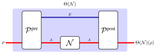
Since is a superchannel, there exist a Hilbert space wih and two CPTP maps , such that [31]
| (89) |
See Fig. 1 for illustration. Assume the decomposition achieves w.r.t. (10), i.e., and each is a CPTP. Substituting this decomposition into (89) yields
| (90) | ||||
| (91) | ||||
| (92) |
where each is a quantum channel. This induces an valid linear decomposition of and thus .
This resource perspective motivates us to investigate the physical implementability of linear maps within the quantum resource theory framework [30] and explore the widely studied robustness measure as well as other channel resource measures [32, 33, 26, 34, 35, 36, 37]. We investigate in Appendix A the proposed robustness measure and show that the two measures, physical implementability and robustness, are actually equivalent in some sense.
3.4 Bounds
In this section, we derive lower and upper bounds on in terms of the commonly used trace norm of the corresponding Choi operator . What’s more, we show explicitly that these bounds are tight. Particularly, the bounds can be saturated by the inverse maps of some well-known quantum channels.
Theorem 10
Let be a -dimensional Hilbert space and Let be an HPTP map in . It holds that
| (93) |
Proof.
To show the first inequality in (93), we make use of the primal SDP (23). Notice that constraint (23b) yields
| (94) |
where the inequality follows from the triangle inequality and the last equality follows from the constraints (23c) and (23d), respectively. Since Eq. (94) holds for arbitrary decomposition satisfying the constraints, it holds in particular for the optimal decomposition and thus
| (95) |
To show the second inequality in (93), recall that is Hermitian and thus diagonalizable. Consider the eigenvalue decomposition
| (96) |
where in the second equality we group the eigenstates by the sign of the corresponding eigenvalues. Let
| (97) | ||||
| (98) | ||||
| (99) | ||||
| (100) |
By construction, we have , , , and . What’s more, since and , the eigenvalues of are always less than , and thus . Similarly, . By Lemma 4 we know the optimal value for decomposing onto CPTN and CPTP are the same, thus we can conclude
| (101) |
3.5 Analytic expression for particular linear maps
In this subsection, we analytically evaluate the physical implementability for some linear maps, which are the inverse map of some practically interesting quantum CPTP maps.
Inverse map of the amplitude damping channel
The qubit amplitude damping channel is given by Kraus operators and , where . That is,
| (102) |
It turns out that is invertible, and the Choi operator of its invertible map has the form
| (103) |
Theorem 11
For , it holds that . What’s more,
| (104) |
Proof.
Remark 3 Note that the previous work [16] has investigated the non-physical implementability of w.r.t. the set of so-called implementable operations444We refer to Eqs. (2) and (3) in [16] for the definition of implementable operations. by imposing both lower and upper bounds on [16, Theorem 3], which has not been tight yet. Our Theorem 11 further strengthens the results on mitigating the amplitude damping noise by concluding that the obtained upper bound is actually optimal even if a larger free set of quantum operations is allowed.
Inverse map of the generalized amplitude damping channel
The generalized amplitude damping (GAD) channel is one of the realistic sources of noise in superconducting quantum processor [38, 39], whose quantum capacity has been studied in [39, 40] It can be viewed as the qubit analogue of the bosonic thermal channel and can be used to model lossy processes with background noise for low-temperature systems. The generalized amplitude damping channel is a two-parameter family of channels described as follows:
| (109) |
where and
| (110) | ||||
| (111) | ||||
| (112) | ||||
| (113) |
Note that when , reduces to the conventional amplitude damping channel. Similar to the amplitude damping channel, is invertible when , and the Choi operator of its inverse map has the form
| (114) |
Lemma 12
For , it holds that
| (115) |
Proof.
We prove (115) by exploring the primal and dual SDP characterizations in Eqs. (23) and (24). We divide the proof into two cases based on the value of , since it influences our constructions of the feasible solutions.
The mixed unitary map.
Let be a set of unitaries in . We say an HPTP map is a mixed unitary map w.r.t. if there exists a set of real numbers such that and
| (120) |
Note that the such defined mixed unitary map can be viewed a natural extension of the mixed unitary channel intensively studied in [20, Chapter 4], by allowing negative coefficients in the mixture. Interestingly, if possesses the orthogonality property, the non-physical implementability of arbitrary mixed unitary map w.r.t. can be evaluated analytically.
Theorem 13
Let be a set of unitaries satisfying the mutual orthogonality condition: , . For arbitrary mixed unitary map w.r.t. of the form (120), it holds that
| (121) |
where is the dimension of the system which is acting on.
Proof.
By the definition of physical implementability, we have . In the following we show that . This, together with the lower bound in Theorem 10, concludes the proof. Notice that
| (122) |
We claim is a set of orthogonal unit vectors, i.e.,
| (123) |
When , the equation can be verified directly. When , it holds that
| (124) | ||||
| (125) | ||||
| (126) | ||||
| (127) |
where the last equality follows from the orthogonality condition. Eqs. (122) and (123) together yield . We are done.
Invertible map of the qudit depolarizing channel.
As an interesting implication of Theorem 13, we can analytically derive the non-physical implementability of the invertible maps of both the depolarizing and dephasing channels. In the following, we first formally define the depolarizing and dephasing channel in the -dimensional Hilbert space . Let which forms a ring w.r.t. to addition and multiplication modulo . The set of discrete Weyl operators in is defined as [20, Section 4.1.2]
| (128) |
where the generalized Pauli operators and are defined as
| (129) |
with the -root of unity . Notice that the set of Weyl operators satisfies the orthogonality condition:
| (130) |
The qudit depolarizing quantum channel , where , is defined in terms of the Weyl operators as
| (131) |
In [16], Takagi gave the optimal sampling cost for qudit quantum channel and qubit dephasing channel, using ad-hoc techniques. Here we show that those bounds can be derived from Theorem 13.
Regarding the depolarizing channel of great practical interests, we have the following.
Lemma 14
For , it holds that .
Invertible map of the qubit dephasing channel.
Let be the Pauli Z operator. Notice that when , the operator define in (129) reduces to . The qubit dephasing quantum channel , where , is defined as
| (134) |
We have the following.
Lemma 15
For , it holds that .
Proof.
Remark 4 Unlike Lemma 14, Lemma 15 does not hold in general for the qudit dephasing channel , where is define in (129). This dues to that does not satisfy the relation in general. It remains as an interesting problem to compute analytically for .
Remark 5 We emphasize that Lemma 14 and Lemma 15 have been shown previously in Theorems 1 and 2 of [16], respectively. In that Ref., the author assumed that the linear map is decomposed w.r.t. the set of implementable operations, which in turn is a strict subset of the set of quantum channels. In this sense, our obtained results enhance the previous ones by specifying the fundamental limit on the physical implementability of these two linear maps.
4 Applications in error mitigation
In this section we endow the proposed physical implementability measure with an operational interpretation within the quantum error mitigation framework as it establishes the lower bound of the sampling cost achievable via the quasiprobability decomposition technique.
4.1 Physical implementability is the sampling cost
In quantum computing, especially in the NISQ era [41], a common computational task is to estimate the expected value for a given observable and a quantum state . Without loss of generality, we may assume to be diagonal in the computational basis, otherwise one can apply a unitary to firstly and then measure in the computational basis. That is, we consider measurement in the form of
| (136) |
If can be prepared perfectly, one can get directly by a sequence of measurements. However, the preparation of inevitably suffers from noise that can be modeled by some CPTP , rendering the value . How can we deal with the noise and recover the expected value anyway? There are many recently proposed error mitigation methods to accomplish this task (see, e.g., [13, 15, 16, 42, 43, 44, 45]).
Since the preparation procedure is given a priori, one feasible way is to perform the invertible map (assumed to exist), yielding
| (137) |
which successfully mitigates the noise. This is quite similar to the quantum channel correction task in the first glance, since we can think of as a correcting procedure.
However, the main problem with (137) is that the invertible map might not be physically implementable, i.e., it is not a CPTP, though we have already shown in Property 1 that is both Hermitian- and trace-preserving. Thus the problem that we are faced with is to physically approximate the effect of an HPTP map, which would unavoidably incur extra computation cost due to approximation. We use the probabilistic error cancellation technique [12, 13, 14, 15, 16] to deal with this issue and it turns out that the incurred computation cost is quantified exactly by the physical implementability measure. The precise error mitigation procedure goes as follows:
-
1.
We optimally decompose into a linear combination of CPTP maps as (10). Then .
-
2.
We iterate the following sampling procedure times. In the -th round where ,
-
2.1.
We sample a CPTP map from with probability . Denote by the sampled coefficient.
-
2.2.
Apply CPTP to , measure each qubit in the computational basis. Denote as the binary string obtained and as the measurement value. Write a random variable
(138) where is the sign function defined as , and , .
-
2.1.
-
3.
Using the data obtained in the second step, we compute the following empirical mean value
(139) -
4.
Output as an estimation of the target expected value .
Now we analyze the efficiency and accuracy of the above estimation procedure. First of all, we show in Lemma 16 that is actually an unbiased estimator of . This justifies the validity of the estimator, as long as is sufficiently large, due to the weak law of large numbers. What’s more, we can apply the Hoeffding inequality to ensure that number of samples in Step 2 would estimate the target expectation value within error with probability no less than :
| (140) | ||||
| (141) |
where follows from the fact that . We can thus identify the unique role of in quantifying the number of rounds required to reach desired estimating precision, empowering the mathematically defined implementability measure an interesting operational meaning.
Lemma 16
The random variable defined in (139) is an unbiased estimator of .
Proof.
One may wonder that the proposed error mitigation setting is a bit unrealistic as the assumption of one can implement all CPTPs perfectly directly remove the necessity of error mitigation in the very first place. To deal with this concern, we describe the setting in more details. In our error mitigation setting, the state preparation and the error mitigation procedures are performed by different parties. Namely, user will prepare the quantum state subject to inevitable quantum noise , while user can perform error mitigation on the received quantum state noiselessly. Since user only knows the error model but has no information about the ideal state that user aims to prepare, he cannot prepare directly by himself.
At the first glance, our setting is different from the more relevant setting where all quantum operations are subject to noise. However, these two settings are in fact closely related, argued as follows. For any invertible quantum noise , we decompose into a linear combination of CPTPs as
| (147) |
Consider the setting where every operation is subject to the noise . The target is to implement a noiseless quantum operation . Notice that
| (148) |
inspiring a feasible method to implement ideally: We firstly sample , and then perform the quantum operation . This quantum operation will be inevitably corrupted by the noise . Statistically, the operation we effectively perform is exactly .
4.2 Properties of the above error mitigation procedure
We explore the operational properties of this error mitigation procedure based on the nice properties and its connection to the sampling cost:
-
•
First, since the physical implementability measure can be computed efficiently via semidefinite programs (cf. Theorem 3), we can estimate the sampling cost of arbitrary linear maps, yielding a feasible way to deal with quantum noise in the NISQ era [41]. However, since the overall sampling cost of a quantum circuit is given by the product of the sampling cost of each gate in the circuit, the overall cost in our error mitigation procedure has an exponential scaling in the number of quantum gates, indicating that error mitigation cannot substitute the role of error correction. Indeed, the proposed error mitigation is an auxiliary method to alleviate quantum errors since NISQ devices do not have enough qubits to support error correcting codes.
-
•
Second, the additivity of w.r.t. tensor product of linear maps (cf. Theorem 6) implies that for parallel quantum noises, global error mitigation has no advantage over local error mitigation, i.e., dealing with quantum noises individually. On the other hand, the subadditivity of w.r.t. composition of linear maps (cf. Theorem 7) implies that for sequential quantum noises, treating them as a whole might be beneficial and reduce the sampling cost, compared to handling these noises one by one. This is intuitive since these quantum noises might cancel mutually in the sequential procedure.
-
•
Third, we obtain the sampling cost analytically for some linear maps which are the inverse map of practically interesting quantum CPTP maps. Prominent examples include the amplitude damping channel (cf. Theorem 11), the generalized amplitude damping channel (cf. Lemma 12), the qudit depolarizing channel (cf. Lemma 14), and the qubit dephasing channel (cf. Lemma 15). These results shed lights on dealing with quantum noises in the NISQ era since they remain as the lower bound of the sampling cost which quasiprobability method may achieve.
5 Conclusions and discussions
In this work, we ask and study the question how can one simulate the action of a general linear map on a quantum state when only quantum operations (CPTP maps) are available. We apply the quasiprobability sampling method and use mathematical tools from semidefinite programming to answer this question, which leads to the first operational quantification of the physical implementability (or non-physicality from another perspective) for general linear maps.
We offered a systematic way to approximate a general linear map, that may not be physically implementable, by decomposing it into a linear combination of physically implementable quantum operations, mathematically characterized by completely positive and trace-preserving maps (CPTPs), motivated by the appealing quasi-probability decomposition technique. We introduced the physical implementability measure of a linear map , which is the least amount of negative portion in the quasi-probability decomposition, as a quantifier of how well can be approximated by CPTPs. We show that is efficiently computable by semidefinite programs. We proved that satisfies many interesting properties such as faithfulness, additivity with respect to the tensor product, and unitary channel invariance. We also derived upper and lower bounds of based on the trace norm of the target linear map’s Choi operator, and obtained analytic expressions for several practical linear maps. Finally, we empowered this measure an operational meaning in the quantum error mitigation task by showing that it establishes the lower bound of the sampling cost achievable via the quasiprobability decomposition technique.
We expect that our proposed framework can find more applications in quantum information and quantum computation. It is also interesting to further explore the structure of invertible qubit HPTP maps and derive an analytic expression for the physical implementability measure. In Section 4, we contributed an efficient method to estimate the expected value in the presence of noise characterized by some noisy quantum channel . This is an important task in quantum computing, especially in the NISQ era. We yearn for new and novel methods for this task.
Acknowledgements.
J. J. and K. W. contributed equally to this work. This work was done when J. J. was a research intern at Baidu Research.
References
- Nielsen and Chuang [2011] Michael A. Nielsen and Isaac L. Chuang. Quantum Computation and Quantum Information. Cambridge University Press, 2011. doi: 10.37686/qrl.v1i1.57.
- Kraus [1983] Karl Kraus. States, effects, and Operations. Springer-Verlag, Berlin, 1983.
- Horodecki et al. [1996] Michał Horodecki, Paweł Horodecki, and Ryszard Horodecki. Separability of mixed states: necessary and sufficient conditions. Physics Letters A, 223(1):1 – 8, 1996. ISSN 0375-9601. doi: 10.1016/S0375-9601(96)00706-2.
- Pechukas [1994] Philip Pechukas. Reduced dynamics need not be completely positive. Physical Review Letters, 73(8):1060, 1994. doi: 10.1103/PhysRevLett.73.1060.
- Carteret et al. [2008] Hilary A Carteret, Daniel R Terno, and Karol Życzkowski. Dynamics beyond completely positive maps: Some properties and applications. Physical Review A, 77(4):042113, 2008. doi: 10.1103/PhysRevA.77.042113.
- Horodecki [2003] Paweł Horodecki. From limits of quantum operations to multicopy entanglement witnesses and state-spectrum estimation. Physical Review A, 68(5):052101, 2003. doi: 10.1103/physreva.68.052101.
- Horodecki and Ekert [2002] Paweł Horodecki and Artur Ekert. Method for direct detection of quantum entanglement. Physical Review Letters, 89(12):127902, 2002. doi: 10.1103/physrevlett.89.127902.
- Fiurášek [2002] Jaromír Fiurášek. Structural physical approximations of unphysical maps and generalized quantum measurements. Physical Review A, 66(5):052315, 2002. doi: 10.1103/physreva.66.052315.
- Korbicz et al. [2008] JK Korbicz, ML Almeida, Joonwoo Bae, M Lewenstein, and A Acin. Structural approximations to positive maps and entanglement-breaking channels. Physical Review A, 78(6):062105, 2008. doi: 10.1103/physreva.78.062105.
- Życzkowski et al. [1998] Karol Życzkowski, Paweł Horodecki, Anna Sanpera, and Maciej Lewenstein. Volume of the set of separable states. Physical Review A, 58(2):883, 1998. doi: 10.1103/physreva.58.883.
- Gurvits and Barnum [2002] Leonid Gurvits and Howard Barnum. Largest separable balls around the maximally mixed bipartite quantum state. Physical Review A, 66(6):062311, 2002. doi: 10.1103/PhysRevA.66.062311.
- Crowder [2015] Tanner Crowder. A linearization of quantum channels. Journal of Geometry and Physics, 92:157–166, 2015. doi: 10.1016/j.geomphys.2015.02.014.
- Temme et al. [2017] Kristan Temme, Sergey Bravyi, and Jay M Gambetta. Error mitigation for short-depth quantum circuits. Physical Review Letters, 119(18):180509, 2017. doi: 10.1103/PhysRevLett.119.180509.
- Howard and Campbell [2017] Mark Howard and Earl Campbell. Application of a resource theory for magic states to fault-tolerant quantum computing. Physical Review Letters, 118(9):090501, 2017. doi: 10.1103/PhysRevLett.118.090501.
- Endo et al. [2018] Suguru Endo, Simon C Benjamin, and Ying Li. Practical quantum error mitigation for near-future applications. Physical Review X, 8(3):031027, 2018. doi: 10.1103/PhysRevX.8.031027.
- Takagi [2020] Ryuji Takagi. Optimal resource cost for error mitigation. arXiv preprint arXiv:2006.12509, 3, 2020. ISSN 2643-1564. doi: 10.1103/physrevresearch.3.033178.
- Vandenberghe and Boyd [1996] Lieven Vandenberghe and Stephen Boyd. Semidefinite Programming. SIAM Review, 38(1):49–95, mar 1996. ISSN 0036-1445. doi: 10.1137/1038003.
- Choi [1975] Man-Duen Choi. Completely positive linear maps on complex matrices. Linear algebra and its applications, 10(3):285–290, 1975. doi: 10.1016/0024-3795(75)90075-0.
- Jamiołkowski [1972] Andrzej Jamiołkowski. Linear transformations which preserve trace and positive semidefiniteness of operators. Reports on Mathematical Physics, 3(4):275–278, 1972. doi: 10.1016/0034-4877(72)90011-0.
- Watrous [2018] John Watrous. The Theory of Quantum Information. Cambridge University Press, 2018. doi: 10.1017/9781316848142.
- Nayak and Sen [2006] Ashwin Nayak and Pranab Sen. Invertible quantum operations and perfect encryption of quantum states. arXiv preprint quant-ph/0605041, 2006.
- Shirokov [2013] Maksim E Shirokov. Reversibility conditions for quantum channels and their applications. Sbornik: Mathematics, 204(8):1215, 2013. doi: 10.1070/sm2013v204n08abeh004337.
- Wigner and Fano [1960] Eugene Paul Wigner and U Fano. Group theory and its application to the quantum mechanics of atomic spectra. AmJPh, 28(4):408–409, 1960. doi: 10.1119/1.1935822.
- Cooney et al. [2016] Tom Cooney, Milán Mosonyi, and Mark M Wilde. Strong converse exponents for a quantum channel discrimination problem and quantum-feedback-assisted communication. Communications in Mathematical Physics, 344(3):797–829, 2016. doi: 10.1007/s00220-016-2645-4.
- Wilde et al. [2020] Mark M. Wilde, Mario Berta, Christoph Hirche, and Eneet Kaur. Amortized channel divergence for asymptotic quantum channel discrimination. Letters in Mathematical Physics, 110(8):2277–2336, aug 2020. ISSN 0377-9017. doi: 10.1007/s11005-020-01297-7.
- Fang et al. [2020] Kun Fang, Xin Wang, Marco Tomamichel, and Mario Berta. Quantum Channel Simulation and the Channel’s Smooth Max-Information. IEEE Transactions on Information Theory, 66(4):2129–2140, apr 2020. ISSN 0018-9448. doi: 10.1109/TIT.2019.2943858.
- Wang et al. [2019a] Xin Wang, Kun Fang, and Marco Tomamichel. On Converse Bounds for Classical Communication Over Quantum Channels. IEEE Transactions on Information Theory, 65(7):4609–4619, jul 2019a. ISSN 0018-9448. doi: 10.1109/TIT.2019.2898656.
- Takagi et al. [2020] Ryuji Takagi, Kun Wang, and Masahito Hayashi. Application of the resource theory of channels to communication scenarios. Physical Review Letters, 124(12):120502, 2020. doi: 10.1103/physrevlett.124.120502.
- Boyd et al. [2004] Stephen Boyd, Stephen P Boyd, and Lieven Vandenberghe. Convex optimization. Cambridge university press, 2004. doi: 10.1017/cbo9780511804441.
- Chitambar and Gour [2019] Eric Chitambar and Gilad Gour. Quantum resource theories. Reviews of Modern Physics, 91(2):025001, 2019. doi: 10.1103/revmodphys.91.025001.
- Chiribella et al. [2008] Giulio Chiribella, Giacomo Mauro D’Ariano, and Paolo Perinotti. Transforming quantum operations: Quantum supermaps. EPL (Europhysics Letters), 83(3):30004, 2008. doi: 10.1209/0295-5075/83/30004.
- Wang and Wilde [2018] Xin Wang and Mark M. Wilde. Exact entanglement cost of quantum states and channels under PPT-preserving operations. arXiv:1809.09592, sep 2018. URL http://arxiv.org/abs/1809.09592.
- Díaz et al. [2018] María García Díaz, Kun Fang, Xin Wang, Matteo Rosati, Michalis Skotiniotis, John Calsamiglia, and Andreas Winter. Using and reusing coherence to realize quantum processes. Quantum, 2:100, oct 2018. ISSN 2521-327X. doi: 10.22331/q-2018-10-19-100.
- Wang et al. [2019b] Xin Wang, Mark M Wilde, and Yuan Su. Quantifying the magic of quantum channels. New Journal of Physics, 21(10):103002, oct 2019b. ISSN 1367-2630. doi: 10.1088/1367-2630/ab451d.
- Yuan et al. [2021] Xiao Yuan, Yunchao Liu, Qi Zhao, Bartosz Regula, Jayne Thompson, and Mile Gu. Universal and operational benchmarking of quantum memories. npj Quantum Information, 7(1):108, dec 2021. ISSN 2056-6387. doi: 10.1038/s41534-021-00444-9.
- Fang and Fawzi [2021] Kun Fang and Hamza Fawzi. Geometric Rényi Divergence and its Applications in Quantum Channel Capacities. Communications in Mathematical Physics, 384(3):1615–1677, jun 2021. ISSN 0010-3616. doi: 10.1007/s00220-021-04064-4.
- Wang and Wilde [2019] Xin Wang and Mark M. Wilde. Resource theory of asymmetric distinguishability for quantum channels. Physical Review Research, 1(3):033169, dec 2019. ISSN 2643-1564. doi: 10.1103/PhysRevResearch.1.033169.
- Chirolli and Burkard [2008] Luca Chirolli and Guido Burkard. Decoherence in solid-state qubits. Advances in Physics, 57(3):225–285, 2008. doi: 10.1080/00018730802218067.
- Khatri et al. [2020] Sumeet Khatri, Kunal Sharma, and Mark M. Wilde. Information-theoretic aspects of the generalized amplitude-damping channel. Physical Review A, 102(1):012401, jul 2020. ISSN 2469-9926. doi: 10.1103/PhysRevA.102.012401.
- Wang [2019] Xin Wang. Pursuing the fundamental limits for quantum communication. arXiv:1912.00931, 67(7):4524–4532, 2019. ISSN 0018-9448. doi: 10.1109/tit.2021.3068818.
- Preskill [2018] John Preskill. Quantum computing in the NISQ era and beyond. Quantum, 2:79, 2018. doi: 10.22331/q-2018-08-06-79.
- Bonet-Monroig et al. [2018] X. Bonet-Monroig, R. Sagastizabal, M. Singh, and T. E. O’Brien. Low-cost error mitigation by symmetry verification. Physical Review A, 98(6):062339, dec 2018. ISSN 2469-9926. doi: 10.1103/PhysRevA.98.062339.
- Endo et al. [2021] Suguru Endo, Zhenyu Cai, Simon C Benjamin, and Xiao Yuan. Hybrid Quantum-Classical Algorithms and Quantum Error Mitigation. Journal of the Physical Society of Japan, 90(3):032001, mar 2021. ISSN 0031-9015. doi: 10.7566/JPSJ.90.032001.
- Wang et al. [2021] Kun Wang, Yu-Ao Chen, and Xin Wang. Measurement Error Mitigation via Truncated Neumann Series. arXiv preprint arXiv:2103.13856, (2):1–14, mar 2021. URL http://arxiv.org/abs/2103.13856.
- Cai [2021] Zhenyu Cai. Multi-exponential error extrapolation and combining error mitigation techniques for NISQ applications. npj Quantum Information, 7(1), 2021. ISSN 20566387. doi: 10.1038/s41534-021-00404-3.
- Harrow and Nielsen [2003] Aram W Harrow and Michael A Nielsen. Robustness of quantum gates in the presence of noise. Physical Review A, 68(1):012308, 2003. doi: 10.1103/PhysRevA.68.012308.
- Vidal and Tarrach [1999] Guifré Vidal and Rolf Tarrach. Robustness of entanglement. Physical Review A, 59(1):141, 1999. doi: 10.1103/PhysRevA.59.141.
- Steiner [2003] Michael Steiner. Generalized robustness of entanglement. Phys. Rev. A, 67:054305, May 2003. doi: 10.1103/PhysRevA.67.054305.
- Brandao [2007] Fernando GSL Brandao. Entanglement activation and the robustness of quantum correlations. Physical Review A, 76(3):030301, 2007. doi: 10.1103/PhysRevA.76.030301.
- Almeida et al. [2007] Mafalda L Almeida, Stefano Pironio, Jonathan Barrett, Géza Tóth, and Antonio Acín. Noise robustness of the nonlocality of entangled quantum states. Physical Review Letters, 99(4):040403, 2007. doi: 10.1103/physrevlett.99.040403.
- Takagi et al. [2019] Ryuji Takagi, Bartosz Regula, Kaifeng Bu, Zi-Wen Liu, and Gerardo Adesso. Operational advantage of quantum resources in subchannel discrimination. Physical Review Letters, 122(14):140402, 2019. doi: 10.1103/PhysRevLett.122.140402.
- Piani and Watrous [2015] Marco Piani and John Watrous. Necessary and sufficient quantum information characterization of einstein-podolsky-rosen steering. Physical Review Letters, 114(6):060404, 2015. doi: 10.1103/physrevlett.114.060404.
- Napoli et al. [2016] Carmine Napoli, Thomas R Bromley, Marco Cianciaruso, Marco Piani, Nathaniel Johnston, and Gerardo Adesso. Robustness of coherence: an operational and observable measure of quantum coherence. Physical Review Letters, 116(15):150502, 2016. doi: 10.1103/physrevlett.116.150502.
- Piani et al. [2016] Marco Piani, Marco Cianciaruso, Thomas R Bromley, Carmine Napoli, Nathaniel Johnston, and Gerardo Adesso. Robustness of asymmetry and coherence of quantum states. Physical Review A, 93(4):042107, 2016. doi: 10.1103/physreva.93.042107.
- Anand and Brun [2019] Namit Anand and Todd A Brun. Quantifying non-markovianity: a quantum resource-theoretic approach. arXiv preprint arXiv:1903.03880, 2019.
- Takagi and Regula [2019] Ryuji Takagi and Bartosz Regula. General resource theories in quantum mechanics and beyond: operational characterization via discrimination tasks. Physical Review X, 9(3):031053, 2019. doi: 10.1103/PhysRevX.9.031053.
- Liu and Winter [2019] Zi-Wen Liu and Andreas Winter. Resource theories of quantum channels and the universal role of resource erasure. arXiv preprint arXiv:1904.04201, 2019.
- Bae et al. [2019] Joonwoo Bae, Dariusz Chruściński, and Marco Piani. More entanglement implies higher performance in channel discrimination tasks. Physical Review Letters, 122(14):140404, 2019. doi: 10.1103/PhysRevLett.122.140404.
- Skrzypczyk and Linden [2019] Paul Skrzypczyk and Noah Linden. Robustness of measurement, discrimination games, and accessible information. Physical Review Letters, 122(14):140403, 2019. doi: 10.1103/PhysRevLett.122.140403.
- Watrous [2017] John Watrous. Semidefinite programming in quantum information (winter 2017). https://cs.uwaterloo.ca/~watrous/CS867.Winter2017/, 2017.
Appendix A Robustness measure
A.1 Definition
As argued around Theorem 9, the set of CPTP maps is treated as the free set when defining the physical implementability measure from the resource theoretic perspective. This motivates us to consider this problem within the quantum resource theory framework [30] and explore the intensively investigated robustness measure [46, 47, 48, 49, 50, 51, 52, 53, 54, 55, 56, 35, 57, 58, 51, 59, 28, 16]. More precisely, Let be an HPTP map, we define the (absolute) robustness of physical implementability of as
| (149) |
Note the minimization is well defined since the completely depolarizing channel is free. Intuitively, quantifies how robust the linear map is against any physical implementation. Alternatively, we can express in terms of its Choi operator as
| (150a) | ||||
| s.t. | (150b) | |||
| (150c) | ||||
| (150d) | ||||
We can further simplify the above program using the trace-preserving condition. Assume the pair achivese in (150). Set , then due to Eq. (150d). Eq. (150b) guarantees that , following from the fact that and Eq. (150c). As so, we can simplify (150) as
| (151a) | ||||
| s.t. | (151b) | |||
| (151c) | ||||
| (151d) | ||||
Correspondingly, the dual SDP is given by
| (152a) | ||||
| s.t. | (152b) | |||
| (152c) | ||||
| (152d) | ||||
One may check that the above SDP satisfies strong duality by the Slater’s theorem [60].
A.2 Relation with the physical implementability
It turns out that the physical implementability measure (10) is closely related to the robustness of physical implementability (149), resembling the relations previously obtained in [14, Eq. (1)] and [16, Eq. (6)].
Theorem 17
Let be an HPTP map. It holds that
| (153) |
Proof.
Note that this theorem can be proved using a similar technique presented in [16, Appendix A]. Here we write down the proof procedure for completeness.
“”: Assume the channel pair achieves , i.e.,
| (154) |
Rearranging the elements leads to , yielding a feasible decomposition of . As so, we obtain from Theorem 3 that
| (155) |
“”: Assume the ensemble achieves (10). Let be the collection of symbols for which the sign of is positive and similarly for . We have and . Set and . By assumption, . Since is trace-preserving, we also have . We can divide the channels into two groups according to the sign of their coefficients:
| (156) | ||||
| (157) | ||||
| (158) |
where and are well-defined quantum channels. This gives . We are done.
Appendix B Proof of Eq. (24)
In this Appendix, we derive the dual program for the primal program given in (23). Recall the primal SDP
| (159a) | ||||
| s.t. | (159b) | |||
| (159c) | ||||
| (159d) | ||||
| (159e) | ||||
Introducing the Lagrange multipliers and , the Lagrange function of this primal SDP is given by
| (160) | ||||
| (161) | ||||
| (162) | ||||
| (163) |
Since , it must hold that otherwise the inner norm is unbounded. Similarly, we have , , and . This leads to the dual SDP
| (164a) | ||||
| s.t. | (164b) | |||
| (164c) | ||||
| (164d) | ||||
| (164e) | ||||
Changing to , we get
| (165a) | ||||
| s.t. | (165b) | |||
| (165c) | ||||
| (165d) | ||||
| (165e) | ||||
Since is Hermitian, so is . Substituting with and renaming the variables , we can rewrite the above program as
| (166a) | ||||
| s.t. | (166b) | |||
| (166c) | ||||
| (166d) | ||||
| (166e) | ||||
Comparing (166) with (24), we are left to show that the inequalities in (166b) and (166c) can be further restricted to equalities. This is true since for any feasible , we can reset it to be . This new solution will make (166b) and (166c) to be equality. At the same time, it satisfies constraints (166d)-(166e) and keep the objective value unchanged.