Possible Resolution of the Hubble Tension with Weyl Invariant Gravity

Abstract

We explore cosmological implications of a genuinely Weyl invariant (WI) gravitational interaction. The latter reduces to general relativity in a particular conformal frame for which the gravitational coupling and active gravitational masses are fixed. Specifically, we consider a cosmological model in this framework that is dynamically identical to the standard model (SM) of cosmology. However, kinematics of test particles traveling in the new background metric is modified thanks to a new (cosmological) fundamental mass scale, $\gamma$, of the model that emerges as an integration constant of the classical field equations. Since the lapse-function of the new metric is radially-dependent any incoming photon experiences (gravitational) red/blueshift in the comoving frame, unlike in the SM. Distance scales are modified as well due to the scale $\gamma$. The claimed $4.4\sigma$ tension level between the locally measured Hubble constant, $H_{0}$, with SH0ES and the corresponding value inferred from the cosmic microwave background (CMB) could then be significantly alleviated by an earlier-than-thought recombination. Assuming vanishing spatial curvature, either one of the Planck 2018 (P18) or dark energy survey (DES) yr1 data sets subject to the SH0ES prior imply that $\gamma^{-1}$ is $O(100)$ times larger than the Hubble scale, $H_{0}^{-1}$. Considering P18+SH0ES or P18+DES+SH0ES data set combinations, the odds against vanishing $\gamma$ are over 1000:1 and 2000:1, respectively, and the model is strongly favored over the SM with a deviance information criterion (DIC) gain $\gtrsim 10$ & $\gtrsim 12$, respectively. The $H_{0}$ tension is reduced in this model to $\sim 1.5$ & $1.3\sigma$, respectively. Allowing for a non-vanishing spatial curvature, $\gamma^{-1}$ halves to $O(50)$ times $H_{0}^{-1}$. The capacity of two other major cosmological probes, baryonic oscillations and type Ia supernovae, SNIa, to distinguish between the models is also discussed. We conclude that the $H_{0}$ tension may simply result from a yet unrecognized fundamental symmetry of the gravitational interaction – Weyl invariance.

1 Introduction

The standard model (SM) of cosmology relies on the diffeomorphism-invariant general relativity (GR). The latter describes gravitational phenomena on solar system scales remarkably well, but is difficult to reconcile with observations on galactic scales unless dark matter (DM) is invoked. Yet on larger scales, the SM of cosmology has proved to be remarkably efficient in explaining a wide range of phenomena on the largest cosmological scales. Nevertheless, it is known to be plagued with a few anomalies, e.g. [1]-[8], assuming that current observational data could be taken as is, with no unaccounted-for systematics or bias of any kind. Yet, it is unlikely that the standard paradigm requires significant revision. However, certain modifications could still be introduced into the model in order to address a few of these anomalies without altering the main features of the SM. They could either be phenomenological or, perhaps more interestingly, derived from revisions of the underlying theory of gravitation.

In general, there appears to be a tension between the cosmic microwave background (CMB) anisotropy at recombination, galaxy weak lensing and Sunyaev-Zeldovich (SZ) cluster observations at redshifts of a few, and local measurements of the Hubble parameter, $H_{0}$. A looming 4.4$\sigma$ tension seems to exist between inferences of $H_{0}$ from cosmological probes, e.g. the Planck 2018 results [9], ACT+WMAP [10] and BOSS galaxy spectrum [11] and measurements from the local Universe, e.g. [12]-[20]. However, a recent independent tip of the red giant branch (TRGB) based local inference of $H_{0}$ yields results which are consistent with both the Planck 2018 (P18) and SH0ES results in better than $2\sigma$ confidence level [21, 22]. It is subject to extinction issues that could potentially bias the inferred $H_{0}$ value, which are still a matter of debate at present [23, 24]. Other concerns about internal inconsistency in type Ia supernovae (SNIa) data sets have been raised recently that call into question the very reality of the ‘Hubble tension’ [25].

Effective distance scale measurements at redshifts of a few are consistent [26, 27] with both cosmological and local inferences of $H_{0}$, possibly hinting towards a monotonic increase of the effective $H_{0}$ value inferred from cosmological scales down to the local Universe. It remains to be seen whether this discrepancy (perhaps at a weaker level than is usually claimed) is corroborated by future independent measurements, e.g. [28-31]. In case it does, there are already a few possible explanations that require extensions of the SM of cosmology, e.g. [32-48], and references in [49, 50, 51].

Yet, another difficulty – albeit not as severe as the Hubble tension but one that has been around for over two decades – faced by the SM of cosmology is the anomalously low power in the lowest multipoles of CMB anisotropy. It has been estimated to be at the $\sim 2\sigma$ discrepancy level with the concordance $\Lambda$CDM model. This tension between the predictions of the SM of cosmology and observations by the WMAP satellite have been latter corroborated by Planck. Extensions of $\Lambda$CDM, e.g. a primordial power spectrum with a sharp infrared cutoff at $k_{c}=O(10^{-4})Mpc^{-1}$ seem to provide a better fit to the WMAP data [52-54].

In this work we explore cosmological implications of a “minimal” modification to GR, i.e. endowing it with Weyl invariance (WI). Applications of this extension of GR to galactic and galaxy cluster scales has been discussed recently in [55]. In the present work a cosmological model is derived in this framework which is spherically-symmetric around any observer. From the standpoint of any observer Newton gravitational constant, $G$, as well as active gravitational masses, have a very mild radial dependence over Hubble scales. In the comoving frame the lapse function of the metric field similarly varies with distance, thereby inducing gravitational red/blueshift. Thus, the rate of redshift of the CMB temperature could be slower than expected based on the standard adiabatic scaling and consequently recombination takes place at higher redshifts that usually thought. As we see below, this configuration seems to offer a statistically significant alleviation of the “Hubble tension” between the CMB-inferred value of $H_{0}$ and the SH0ES prior.

This is in contrast to a few recent works [56-59] that adopted a phenomenological SM-based approach in which $T_{0}$, the locally measured CMB temperature, is a free parameter. Imposing the local $H_{0}$ prior results in a lower-than-FIRAS value for $T_{0}$. The impact on $H_{0}$ in this case comes from the late integrated Sachs Wolfe (ISW) effect and CMB lensing by the large scale structure (LSS).

The paper is structured as follows. The cosmological model is derived in section 2. The data sets used, the analysis and results are described in section 3, followed by a summary in section 4. A specific WI generalization version of GR is described is the Appendix (although we stress here that our analysis equally-well applies to any WI theory of gravity that admits a homogeneous and isotropic metric solution). Throughout, we adopt a mostly-positive signature for the spacetime metric $(-1,1,1,1)$, with the speed of light $c$ set to unity.

2 Cosmological model

Diffeomorphism invariance that underlies GR embodies the idea that the physical laws of nature do not depend on the state of the observer. Another possible symmetry of gravitation, at least in principle, is invariance under local change of units. The fundamental length and mass units in GR are the Planck length/mass and active gravitational masses (of e.g. particles such as the electron, proton, etc.). Based on early terrestrial experiments and observations in the solar system these quantities are taken to be universal constants in GR. However, it is not experimentally/observationally excluded that these may slightly vary over galactic or cosmological scales. A theory of gravitation that retains the merits of GR while still allows for flexible units of length/mass would actually be a locally scale invariant, i.e. WI, version of GR.

The proposed model is obtained from the GR-based Friedmann-Robertson-Walker (FRW) model via a particular Weyl transformation, essentially a local rescaling of fields by their mass/length dimension such that dimensionless ratios of fields remain invariant. It is assumed that the SM of particle physics is unchanged. In particular, the latter does not possess WI as it contains the electroweak and quantum chromodynamics (QCD) mass scales. Specifically, Weyl transformation applied to a metric $g_{\mu\nu}$ amounts to local stretching/squeezing, i.e. $g_{\mu\nu}\rightarrow\Omega^{2}(x)g_{\mu\nu}$, where $\Omega(x)>0$ is an arbitrary well-behaved spacetime-dependent function. Therefore, length scales are locally rescaled by $\Omega(x)$. This implies that mass scales transform as $m\rightarrow m/\Omega(x)$, and quantities such as energy density $\rho(x)$ and pressure $P(x)$ transform $\propto\Omega^{-4}$. WI of a theory implies that the equations describing it, or equivalently the action from which the latter are derived, are invariant under such local rescalings.

The masses that appear in the Einstein-Hilbert (EH) action are the active gravitational mass $M_{act}$ that sources the gravitational interaction and the Planck mass $m_{P}$ ($m_{P}\propto G^{-1/2}$). Consequently, the quantity that controls the strength of the gravitational interaction, $GM_{act}$, scales $\propto\Omega(x)$. The assumption that inertial masses, generated by the SM of particle physics, are fixed but active gravitational masses are spacetime-dependent in this model does not conflict with the equivalence principle (aside from the fact that the latter has never been directly tested on cosmological scales anyway [60]). The latter holds whenever the passive gravitational mass is proportional to the inertial mass. We indeed make this assumption here and set the proportionality constant to unity.

Assuming that GR (with $G=constant$ and $M_{act}=constant$) represents just one choice out of infinitely many conformally-related possibilities allowed by nature then any metric field that satisfies the Einstein equations could be Weyl transformed by means of an arbitrary $\Omega(x)$ into new metrics. There is no a priori preference to any particular conformal frame, and only observations can select the “appropriate” frame, much like GR prefers no particular coordinate system, i.e. the state of the observer; this information can only be extracted from observations. We stress that the proposed model is based on a spacetime metric which is obtained from the FRW metric via a combined Weyl and coordinate transformations. While null geodesics followed by CMB photons are blind to the former they are not invariant under the latter type of transformations.

We start with the FRW metric in GR

$$ds^{\prime 2}=a^{2}(t)\left[-\frac{dt^{2}}{a^{2}}+\frac{dr^{\prime 2}}{1-Kr^{\prime 2}}+r^{\prime 2}(d\theta^{2}+\sin^{2}\theta d\varphi^{2})\right],$$ (2.1)

where $K$ is the spatial curvature parameter, and we use standard spherical coordinates. The scale factor $a(t)$ satisfies the Friedmann equation, and $t$ is cosmic time. Since the observable Universe appears to be very nearly isotropic around us we seek a spherically-symmetric solution described by the following static line element

$$ds^{2} = a^{2}[-A(r)d\eta^{2}+A^{-1}(r)dr^{2}+r^{2}(d\theta^{2}+\sin^{2}\theta d\varphi^{2})],$$ (2.2)

where in general $r$ differs from $r^{\prime}$, and conformal and cosmic time coordinates are related via $d\eta=dt/a(t)$. This is of course not the most general spherically-symmetric metric for it could be multiplied by any $\Omega(r)$ without spoiling the symmetry. Although any spherically symmetric solution can always be reduced to the “canonical” form, eq. (2.2), via combined coordinate and Weyl transformations, it does not have to be, and null geodesics do depend on the underlying coordinate system. Since the latter reflects the state of the observer (which is a priori arbitrary) then, in general, different choices of underlying coordinate frames could result in observationally distinguishable models. It should be also realized that by virtue of the cosmological principle spacetime is spherically-symmetric around any observer, i.e. the origin of spherical coordinates system can be chosen at an arbitrary observer. This is manifested in the framework adopted in this work by the fact that dimensionless quantities of conformal weight 0 are purely time dependent, as we see below.

It is instructive at this point to recover the phenomenon of cosmological redshift in the comoving frame. In the SM (assuming vanishing spatial curvature), where $A=1$, eq. (2.2) is conformally related to $ds^{2}=-dt^{2}/a^{2}(t)+dr^{2}+r^{2}(d\theta^{2}+\sin^{2}\theta d\varphi^{2})$, and since null geodesics are blind to conformal transformations then light is blue/redshifted by virtue of the standard gravitational blue/redshift effect. The latter is described by the gravitational shift formula $\nu_{e}/\nu_{o}=\sqrt{g_{tt}(r_{o})/g_{tt}(r_{e})}$, where $\nu$ is the frequency, and the subscripts ‘e’ and ‘o’ refer to emitted and observed quantities, respectively. Defining $a(t)\equiv a_{0}/(1+z)$ the standard relation $\nu_{e}=\nu_{o}(1+z)$ readily follows. In the more general case described by eq. (2.2) the lapse function $g_{tt}\propto A(r)$ is r-dependent. Consequently, radially incoming photons experience additional red/blueshift over the standard cosmological redshift $\nu_{e}/\nu_{o}=(1+z)$. In the cosmological context, and in the special case $A=1-\frac{\Lambda r^{2}}{3}$ (with $a(t)=1$ and $\Lambda$ a cosmological constant), this r-dependent effect has been historically known as the “de-Sitter Effect” [61-65], predicted to be observed towards, e.g. globular clusters [65], when the static de-Sitter model was the model of choice in the pre-FRW model era. This immediately implies that the CMB temperature scaling with redshift, $T_{CMB}(z)$ is different from that in the SM and therefore recombination could have taken place at higher or lower redshifts than naively expected based on the FRW model alone ($z_{\star}\approx 1089$). Consequently, an FRW-model-based (i.e. eq. 2.1) inference of $H_{0}$ (and possibly other cosmological parameters as well) relying on the temperature anisotropy and polarization of the CMB is biased if spacetime is genuinely described by eq. (2.2). This property of the metric described by eq. (2.2), at least in principle, opens up the possibility of reconciling the “Hubble tension” between the locally-inferred $H_{0}$ value, and the value inferred from the CMB, i.e. at $z_{\star}\approx 1089$.

It has been shown recently that by relaxing the local FIRAS constraint and promoting the locally measured CMB temperature, $T_{0}=2.72548\pm 0.00057\ K$ [66], to a free parameter, still within the “FRW framework”, along with imposing the SH0ES constraint on $H_{0}$ favors a lower $T_{0}$ than the “canonical” FIRAS value [56-59]. This latter picture is of course inconsistent with the FRW framework as the locally measured FIRAS value is the most precisely measured cosmological parameter. Nevertheless, it illustrates that the $H_{0}$ tension between CMB and locally inferred values is correlated with a similar tension in $T_{0}$ (albeit with lower statistical significance). In contrast, the model discussed here provides us with a mechanism for evolving $T_{CMB}(z)$, and not only that – it also relates temperature evolution to the spatial curvature parameter $\Omega_{k}$ (in addition to a new model parameter, $\gamma$, that we introduce below). Thus, the intricate interplay between $H_{0}$, $\Omega_{k}$, and in general any other cosmological parameter that affects conformal distance, and the effective $T_{CMB}(z)$, is self-consistently determined by fitting the model described by eq. (2.2) to observational data, and is not an ad hoc imposition. This is done without having to ignore the FIRAS value; $T_{CMB}(z;\{p\})$ evolves smoothly from the FIRAS value here and now, $T_{0}$, as a function of a few cosmological parameters (collectively denoted here $\{p\}$) all the way to recombination and beyond.

In general, the angular diameter distance obtained from eq. (2.2) is different from that obtained from eq. (2.1), with obvious implications for, e.g. calculation of the CMB anisotropy and polarization spectra, as well as galaxy correlation spectra. In addition, baryonic oscillations (BAO)-based inference of the scale at decoupling, which proved to be instrumental in establishing global spatial flatness [9], evidently depends on the metric used, for the BAO scale is conventionally quoted in Mpc units whereas angular correlations are the quantities actually measured at various redshifts; converting these observables to physical scales inevitably involves assumptions about the underlying metric, and by default it is the one described by eq. (2.1), and not eq. (2.2).

Applying a Weyl transformation $ds^{2}=\Omega^{2}(r^{\prime})ds^{\prime 2}$ along with a coordinate transformation $r^{\prime}\rightarrow r$ to relate eqs. (2.1) & (2.2) the following set of conditions is obtained

$$\Omega^{2} = A(r)$$

$$\frac{\Omega^{2}dr^{\prime 2}}{1-Kr^{\prime 2}} = \frac{dr^{2}}{A(r)}$$

$$\Omega = r/r^{\prime},$$ (2.3)

from the $g_{tt}$, $g_{rr}$ & $g_{\theta\theta}$ terms, respectively. Combined, these constraints result in $\frac{dr^{\prime}}{r^{\prime 2}\sqrt{1-Kr^{\prime 2}}}=\pm\frac{dr}{r}$, and the requirement that $dr^{\prime}\rightarrow dr$ at the observer, $r=0$, selects the positive sign. Integration then results in

$$A(r)=\Omega^{2}=(r/r^{\prime})^{2}=\left(1+\frac{\gamma r}{2}\right)^{2}+Kr^{2}=1+\gamma r-\frac{\Lambda}{3}r^{2},$$ (2.4)

where $\gamma$ is a new model parameter (that emerges as an integration constant) of units $length^{-1}$. Since $\gamma$ is an integration constant it can a priori assume arbitrary values. In the last equality we defined $\frac{\gamma^{2}}{4}+K\equiv-\frac{\Lambda}{3}$ to emphasize that the metric is asymptotically de Sitter or anti-de Sitter with an effective cosmological constant $\Lambda$. In the special case $K=0$, eq. (2.4) reduces to $\frac{1}{r}=\frac{1}{r^{\prime}}-\frac{\gamma}{2}$. In the case $\gamma<0$ the radial coordinate $r$ is bounded, $r<\frac{2}{|\gamma|}$, with obvious implications for large scale observables in, e.g. the CMB anisotropy. We note that a static version of eq. (2.2), i.e. with $a(t)=1$, and with $A(r)$ given by eq. (2.4), has been derived within the framework of another WI theory, fourth-order WI gravity, and proposed as a solution to the galactic rotation curves problem [67-70]. In fourth-order WI gravity, much like in any other WI version of GR (e.g the WI scalar-tensor theory described in the Appendix), there is a new functional degree of freedom (whose description in general involves an unlimited number of parameters) which in the highly (spherically) symmetric case described by eq. (2.2) reduces to a single new parameter, $\gamma$. This fact is reflected in eq. (2.4) where the conformal factor $\Omega$, which a priori is a free scalar function, is parameterized by only two parameters [where $K$ was already introduced in the FRW metric described by eq. (2.1)]. Much like in GR where the cosmological constant can be viewed as an integration constant of the Einstein equations, so is $\gamma$ that appears in WI extensions of the FRW metric only inferred from observations – the theory is a priori completely agnostic about its empirical value. Clearly, the actions that describe the WI theories explored in [67] and in the Appendix are scale-free, but integration of the associated classical field equations does require dimensional integration constants.

Starting from the FRW metric, eq. (2.1), we generated a new spherically-symmetric cosmological solution with a metric of the form described eq. (2.2). If WI is indeed a symmetry of gravitation then mass scales (i.e. inverse length scales) transform $\propto\Omega^{-1}\propto A^{-1/2}(r)$. We note that in the special case $\gamma=0$ & $K=-\frac{\Lambda}{3}$ the new metric, eq. (2.2), is conformally related to static de-Sitter metric (where $K<0$, i.e. $\Omega_{k}>0$ corresponds to $\Lambda>0$, i.e. $\Omega_{\Lambda}>0$).

Calculation of the Ricci curvature scalar associated with the metric described by eq. (2.2) in the comoving frame with $A(r)$ given by eq. (2.4) results in $R=-12(K+\frac{\gamma^{2}}{4})-\frac{6\gamma}{r}$. Unlike in the case of the FRW metric, where $R=6K$ is a fixed constant, the curvature scalar associated with the spacetime described by eq. (2.2) diverges at $r=0$. This divergence is not a problem for the model as $R$ in a WI theory is not an observable; while it is invariant under coordinate transformations it is not blind to Weyl transformations. Under a conformal transformation $g_{\mu\nu}\rightarrow\Omega^{2}g_{\mu\nu}$ the Ricci scalar transforms as $R\rightarrow\Omega^{-2}\left(R-6\frac{\Box\Omega}{\Omega}\right)$, where the d’Alambertian $\Box$ is calculated in the old metric. Since the definition of $R$ involves derivatives of fields (in this case – the metric field) it does not have a well-defined conformal weight; It can well vanish in one conformal frame and diverge at another frame. This is analogous to the fact that in GR only tensor quantities of well-defined rank are meaningful observables, and in particular only scalars are invariant observables. For example, since the connection (Christoffel symbol) is not a tensorial quantity (i.e. it does not transform homogeneously under coordinate transformations) it can assume non-vanishing values (or even diverge) in one coordinate system, and nevertheless be set to vanish locally by means of coordinate transformations in a second system. It is therefore not an observable in GR. In practice, the singularity in $R$ of eq. (2.2) is offset by, e.g. a singularity in $\Box G$. Therefore, $R$ is not an observable as it has units $length^{-2}$, and a “dynamical” unit of length can be found in terms of which it is everywhere finite. This length unit is the Planck scale.

Within the formalism described in the previous section, the proposed cosmological model is obtained from the SM via a combined coordinate and conformal transformations which are given by eq. (2.4), $\Omega^{2}=(r/r^{\prime})^{2}=1+\gamma r-\frac{\Lambda}{3}r^{2}$. Consequently, $m_{pl}\rightarrow m_{pl}(1+\gamma r-\frac{\Lambda}{3}r^{2})^{-1/2}$, and $m_{pl}$ in the new frame, eq. (2.2), is now r-dependent as measured by any observer. As mentioned below eq. (2.4), the metric describing our model has a divergent curvature $R=-12(K+\frac{\gamma^{2}}{4})-\frac{6\gamma}{r}$. This divergence does not go away even if we consider the dimensionless combination $R/|\phi|^{2}$. However, WI quantities must have a vanishing conformal weight by definition. For example, in one specific WI theory of gravitation (see Appendix) such a zero conformal weight combination involving $R$ is, e.g.

$$\frac{-|\phi|^{2}R+6{\rm Re}(\phi\Box\phi^{*})}{|\phi|^{4}}=\frac{3T_{M}}{|\phi|^{4}},$$ (2.5)

where $\phi$ is a complex scalar field in a WI scalar tensor theory of gravitation. Since $\frac{T_{M}}{|\phi|^{4}}$ is invariant under conformal transformation, and is $\propto\rho_{M}(\eta)$ in the SM, it is clear that it is purely time dependent, and the divergence of $R$ at $r=0$ is exactly offset by a similar divergence sourced by variations of the scalar field. The latter is canceled by a similar divergence of the $\phi\Box\phi^{*}$ term, i.e. gradients of the scalar field (i.e. $G$ or equivalently $m_{pl}$, and $M_{act}$).

Incoming radial null geodesics are described in the new metric, eq. (2.2), by

$$d\eta=-\frac{dr}{A(r)}=-\frac{dr}{(1+\frac{\gamma r}{2})^{2}+Kr^{2}}.$$ (2.6)

It is useful to introduce the dimensionless parameter $\kappa\equiv(K+\frac{\gamma^{2}}{4})H_{0}^{-2}=\alpha^{2}-\Omega_{k}$, in terms of which eq. (2.6) is rewritten as

$$H_{0}d\eta=-\frac{dx}{1+2\alpha x+\kappa x^{2}},$$ (2.7)

where $x\equiv H_{0}r$, $\alpha\equiv\gamma/(2H_{0})$, and as usual $\Omega_{k}\equiv-K/H_{0}^{2}$. The metric is asymptotically de-Sitter if the $2\alpha x$ term is ignored, so even in that case we already expect a “de-Sitter effect” in addition to the standard scaling of temperature with redshift, $T_{CMB}(z)=T_{0}(1+z)$.

Integration of eq. (2.7) results in

$$H_{0}r(z)=\left\{\begin{array}[]{ll}\frac{\sqrt{-\Omega_{k}}}{\kappa}\left[\frac{\sqrt{-\Omega_{k}}\sin(\sqrt{-\Omega_{k}}\mathcal{D})+\alpha\cos(\sqrt{-\Omega_{k}}\mathcal{D})}{\sqrt{-\Omega_{k}}\cos(\sqrt{-\Omega_{k}}\mathcal{D})-\alpha\sin(\sqrt{-\Omega_{k}}\mathcal{D})}\right]-\frac{\alpha}{\kappa}&;\Omega_{k}<0\\ \\ \frac{\mathcal{D}}{1-\alpha\mathcal{D}}&;\Omega_{k}=0\\ \\ \frac{\sqrt{\Omega_{k}}}{\kappa}\left[\frac{-\sqrt{\Omega_{k}}\sinh(\sqrt{\Omega_{k}}\mathcal{D})+\alpha\cosh(\sqrt{\Omega_{k}}\mathcal{D})}{\sqrt{\Omega_{k}}\cosh(\sqrt{\Omega_{k}}\mathcal{D})-\alpha\sinh(\sqrt{\Omega_{k}}\mathcal{D})}\right]-\frac{\alpha}{\kappa}&;\Omega_{k}>0\ \&\ \kappa\neq 0\\ \\ (2\sqrt{\Omega_{k}})^{-1}\left[\exp(2\sqrt{\Omega_{k}}\mathcal{D})-1\right]&;\Omega_{k}>0\ \&\ \kappa=0,\\ \end{array}\right.$$ (2.15)

where

$$\mathcal{D}(z;\{\Omega_{i,0}\}) \equiv H_{0}(\eta_{0}-\eta)=\int_{0}^{z}\frac{dz^{\prime}}{E(z^{\prime})},$$

$$E^{2}(z^{\prime}) \equiv \sum_{i}\Omega_{i,0}(1+z^{\prime})^{3(1+w_{i})},$$ (2.16)

is standard in the SM of cosmology, and $\{\Omega_{i,0}\}$ collectively stands for the $\Omega_{i,0}$ which are the respective energy densities at present of the i’th species in critical density units [not to be confused with the conformal factor $\Omega(x)$ of eqs. 2.3], including $\Omega_{k}$ with an effective equation of state (EOS) $w_{k,eff}=-1/3$. Already at this point it is clear from eq. (2.8) in the case $\Omega_{k}=0$ that effectively

$$H_{0,eff}(z)=H_{0}[1-\alpha\mathcal{D}(z)],$$ (2.17)

is lower than $H_{0}$ if $\alpha>0$. In other words, the inferred Hubble parameter, $H_{0}$, is effectively running with redshift, and is lower (if $\alpha>0$) when inferred from higher redshift probes than is locally measured, which can qualitatively explain the discrepancy between the $H_{0}$ values inferred by local and cosmological probes. This picture is consistent with the evolution of frequency/temperature that we consider below, and lies at the heart of the proposed resolution of the Hubble tension. This argument is not changed qualitatively when $\Omega_{k}$ is allowed to be non-vanishing.

This cosmological model is spatially finite for any $\Omega_{k}>0$ (opposite to the standard FRW which is finite when $\Omega_{k}<0$) and is infinite insofar $\Omega_{k}<0$. Setting $A(r)=0$ we obtain two solutions, $r_{\pm}=-\frac{1}{2H_{0}(\alpha\pm\sqrt{\Omega_{k}})}$. Indeed, positive roots, i.e. horizons, exist only if $\Omega_{k}>0$. In case $\alpha<0$ it exists if $\kappa>0$. Another root exists if $\alpha<\sqrt{\Omega_{k}}$. It is easy to see that eq. (2.8) satisfies $r(z)\leq r_{\pm}$ at any redshift irrespective of the values of $\Omega_{i}$’s. From this we see that a finite $r$ requires $\Omega_{k}>0$, exactly opposite to the SM. This is not surprising given the sign-flip of $K$ seen in eq. (2.4) and comparison of eqs. (2.1) & (2.2).

Since mass/energy scales $\propto A(r)^{-1/2}$ where $A(r)=1+2\alpha x+\kappa x^{2}$, employing eq. (2.8) frequencies then evolve on the light cone as

$$\frac{\nu(z)}{\nu_{0}(1+z)}=\left\{\begin{array}[]{ll}\cos(\sqrt{-\Omega_{k}}\mathcal{D})-\frac{\alpha}{\sqrt{-\Omega_{k}}}\sin(\sqrt{-\Omega_{k}}\mathcal{D})&;\Omega_{k}<0\\ 1-\alpha\mathcal{D}&;\Omega_{k}=0\\ \cosh(\sqrt{\Omega_{k}}\mathcal{D})-\frac{\alpha}{\sqrt{\Omega_{k}}}\sinh(\sqrt{\Omega_{k}}\mathcal{D})&;\Omega_{k}>0\ \&\ \kappa\neq 0\\ \exp(-\alpha\mathcal{D})&;\Omega_{k}>0\ \&\ \kappa=0.\end{array}\right.$$ (2.22)

We stress that dimensionless ratios of fields are independent of the conformal factor $\Omega(x)$, i.e. they obtain their SM values. eq. (2.11) applies to $m/m_{0}$ (where $m$ either the Planck mass or any active gravitational mass) as well, as would be expected based on the mass dimension of frequency and masses.

Assuming that both $|\Omega_{k}|\ll 1$ and $|\alpha|\ll 1$ it then follows from eq. (2.11) that the CMB temperature evolves as

$$T(z)\approx T_{0}(1+z)[1-\alpha\mathcal{D}(z;\{\Omega_{i,0}\})],$$ (2.23)

where ${D}(z;\{\Omega_{i,0}\})$, defined in eq. (2.9), is a function of redshift and the various contributions to the total energy density budget via their respective $\Omega_{i}$. Assuming that the cosmological parameters do not deviate significantly from their concordance model values we estimate $\mathcal{D}(z_{\star})\gtrsim 3$ at recombination, i.e. $T_{\star}/T_{0}\approx(1+z_{\star})(1-3\alpha)$, where $T_{\star}$ is the CMB temperature at $z_{\star}$, the recombination redshift. From the ratio of eqs. (2.12) & (2.10) and the expectation that $T(z_{\star})$ depend on atomic physics which is unchanged here since the SM of particle physics is assumed to hold as is it follows that for fixed $H_{0}$ & $T_{0}$ then $(1+z_{\star})^{-1}\propto H_{0,eff}(z_{\star})$ irrespective of the sign of $\alpha$. A higher $z_{\star}$ then implies a lower $H_{0,eff}$. Therefore, $\alpha>0$, i.e. a lower temperature in comoving frame at a given $z$, implies that recombination has taken place at a higher $z_{\star}$ than expected based on the FRW model, and consequently a lower $H_{0,eff}$. This should be compared with the $T_{0}-H_{0}$ anti-correlation reported in [56-59] where $T_{0}$ was a free parameter (and $T_{\star}$ was essentially fixed as emphasized in [59]).

From the foregoing discussion it should be clear that at least CMB anisotropy and polarization, galaxy correlations, and BAO, can be used in principle to distinguish between the SM and the model proposed here. However, this turns out not to be the case for the SNIa probe. Indeed, since the luminosity $\propto dE/dt\propto\nu^{2}$ is proportional to $D_{L}^{2}$ then it follows that $D_{L}\rightarrow D_{L}\nu(z)/\nu_{0}$ where $\nu(z)/\nu_{0}$ is given by eq. (2.11). Therefore, $D_{L}(z)=(1+z)^{2}L_{A}(z)\nu(z)/\nu_{0}$, where $L_{A}(z)$ is the angular diameter distance. Combining this with eqs. (2.8) & (2.11) it is then clear that the luminosity distance $D_{L}(z)$ reduces to exactly the SM expression. It should be realized that this conclusion is unique to the specific model considered in the present work. While it is true that null geodesics are insensitive to Weyl transformations of the SM metric and therefore angular diameter distances $L_{A}(z)$ are unchanged, frequencies do rescale as $\nu\rightarrow\nu/\Omega(x)$ and consequently the product $L_{A}(z)\nu(z)$ can be used in general to determine the conformal frame. In addition, null geodesics do change under coordinate transformations, and these two effects happen to cancel each other out in the specific model considered here. This conclusion is consistent with the results reported from our model comparison analysis in the next section; when the SNIa data set is included in the analysis the improvement in the fit offered by this extended model is statistically weakened in comparison to the same model applied to the CMB and dark energy survey (DES) data sets (subject to the SH0ES prior).

As discussed above, the SM and the conformally-related model considered here are dynamically identical, by construction. This statement applies at both the background and perturbations level. As we just saw, kinematics of test particles traveling on the two background metrics differ. In general, this is the case in the perturbed metrics as well. Since the CMB photons at around decoupling from the plasma can no longer be considered a perfect fluid they are described by kinetic theory instead, via the collisional Boltzmann equation. The latter is integrated along null geodesics between subsequent collisions with free electrons, and could be potentially affected by the modified kinematics. However, as the new parameter $\alpha=\gamma/(2H_{0})$ controls the departure of geodesics in the new model from their counterparts in the SM, and since with available observations $|\alpha|<0.01$ as we see in the next section, then we conclude that this effect is second order at best. In addition, the allowed k-mode values for linear perturbations could be potentially restricted in the model considered here unlike in flat or open FRW models. In case that $\gamma<0$ (i.e. $\alpha<0$) the radial coordinate $r$ is bounded by $r_{max}=\frac{2}{|\gamma|}$ and there is an infrared cutoff at the Fourier modes $k_{min}=\pi|\gamma|$ even in case that $K=0$. In principle, this could alleviate the low power anomaly on the largest cosmological scales, as in [52-54]. In our analysis, we ignore the cutoff caused by $\gamma<0$. Given the relatively low statistical weight of the largest scales, this is justified in retrospective by the analysis results (described in the next section) that point towards a clear preference for $\gamma>0$ in case that SH0ES prior is imposed, and vanishing $\gamma$ otherwise.

3 Analysis and results

The data sets used in the analysis are the same as those included in CosmoMC 2019, and used in, e.g. [58]. Five different data set combinations are considered in the present work: P18 alone, P18+DES, P18+BAO, P18+Pantheon and P18+BAO+Pantheon. Specifically, the P18 dataset includes temperature anisotropy, polarization and lensing extraction data, the DES 1yr (cosmic shear, galaxy auto-and cross-correlations), BAO (compilation from BOSS DR12, MGS, and 6DF), Pantheon (catalog of 1048 SNIa).

These data set combinations are considered with and without the SH0ES prior. Whereas the value deduced by the SH0ES team [14], $H_{0}=74.03\pm 1.42$ km/(s Mpc), formally represents the most precise local measurement of $H_{0}$ to date, it also lies on the far end of a range of local measurements that indeed results in systematically higher $H_{0}$ values than inferred from P18. Therefore, it is not entirely unlikely that this result in biased to some extent [24, 71].

It was mentioned in section 2 that BAO data reduction process is likely biased towards the SM, and that SNIa data is blind to any difference between the specific model considered here and the SM. Therefore, we will be mainly concerned with either the P18 or DES yr1 data sets with the SH0ES prior on $H_{0}$ either included or excluded. We also consider the case of either flat space prior or not. These are our baseline data sets.

Our model is parameterized by the standard cosmological parameters $\Omega_{b}h^{2}$, $\Omega_{c}h^{2}$, $\Omega_{k}$, $\theta_{MC}$, $\tau$, $A_{s}$ & $n_{s}$, as well as a new dimensionless parameter $\alpha$, and a few additional likelihood parameters in case of P18, DES 1yr, BAO and the (SNIa catalog) Pantheon data sets. Here, $\Omega_{b}$, $\Omega_{c}$, and $\Omega_{k}$ are the energy density of baryons, cold dark matter (CDM) and the energy density associated with spatial curvature in critical density units, respectively. The reduced Hubble constant is $h\equiv H_{0}/100$, where $H_{0}$ is given in km/(s Mpc) units, $\theta_{MC}$ as usual is the ratio of the acoustic scale at recombination and the horizon scale back to $z_{\star}$, $\tau$ is the optical depth at reionization, and $A_{s}$ & $n_{s}$ are the amplitude and tilt of the primordial power spectrum of scalar perturbations, respectively. Flat priors used in the present analysis for the cosmological parameters are shown in table 1.

Parameter	Fiducial	prior
$\Omega_{b}h^{2}$	0.0221	[0.005, 0.1]
$\Omega_{c}h^{2}$	0.12	[0.001, 0.99]
$100\theta_{MC}$	1.0411	[0.5, 10]
$\tau$	0.06	[0.01, 0.8]
$\ln(10^{10}A_{s})$	3.1	[1.61, 3.91]
$n_{s}$	0.96	[0.8, 1.2]
$\Omega_{k}$	0	[-0.3, 0.3]
$\alpha$	0	[-0.3, 0.3]

Table 1: The basic cosmological parameters, their fiducial values, and flat priors are specified. The derived value of $H_{0}$ was constrained to the interval [10, 100] km/(s Mpc).

Sampling from posterior distributions is carried out with a Gelman-Rubin convergence criterion [72] $R-1<0.02$, and the deviance information criterion (DIC) is adopted for model comparison [73]. A DIC gain $|\Delta DIC|$ (compared to a reference model) of $<$1, 1.0-2.5, 2.5-5.0, and $>$5.0 indicates inconclusive, weak/moderate, moderate/strong, or decisive evidence in favor of the extended model over the reference model, respectively [74].

In this work we compare the fit of four different cosmological models to various combinations of the data sets. In addition to the flat SM, we refer to the SM with $\Omega_{k}\neq 0$ as ‘SM+K’. Both models are described by eq. (2.1). The other two models are described by eq. (2.2) where $A(r)$ is given by eq. (2.4); the case $\alpha\neq 0$ & $K=0$ is referred to as Model-I (“MI”), and the case $\alpha\neq 0$ & $K\neq 0$ is referred to as Model-II (“MII”). For model comparison purposes the reference models for MI & MII are SM & SM+K, respectively.

In spite of comprehensive robustness tests that BAO has passed, e.g. [75-79], it is clear that going from the observed angular correlations on the sky to the physical acoustic scale at the drag epoch, $r_{d}$, involves the use of a metric, and clearly this has never been the one described by eq. (2.2). Therefore, we expect that the standard FRW-based data reduction involved in BAO data analyses could be biased towards $\Omega_{k}=0$ & $\alpha=0$ [as can be appreciated from comparison of eqs. (2.1) & (2.2)]. This is an important observation given the instrumental role played by BAO in establishing global flatness in light of the recent P18 results that by themselves favor a closed Universe [9]. In comparison, P18 data is given in terms of angular power spectra which are independent of any fiducial model.

Therefore, although we do consider data set combinations that involve BAO in our analysis which is summarized in tables 2-4 below, we caution that a priori these might be biased towards a flat FRW model (i.e. favoring smaller $|\alpha|$ and $|\Omega_{k}|$ simply due to adopting a GR-based cosmological model, eq. 2.1).

DIC values for the SM, MI, SM+K & MII models are shown in table 2 for each of the data set combinations with or without the SH0ES prior (first or last five lines, respectively). Also shown are $\Delta DIC$ values for MI with respect to the SM, and MII with respect to SM+K, respectively. It is clear from table 2 that MI is decisively favored over the SM in cases where the SH0ES prior is imposed. Spatial flatness is theoretically favored by the SM with inflation, as well as by most alternative scenarios of the very early Universe. In this context it should be stressed that while $\Omega_{k}$ is dynamically suppressed relative to nonrelativistic energy densities, e.g. of the CDM, in an expanding universe, the parameter $\gamma$ is genuinely a constant of integration obtained by a coordinate transformation (eq. 2.4), unlike $K$ it does not appear in the (dynamical) field equation (the Friedmann equation essentially) but rather only affects the kinematics, i.e. the geodesic equations, and therefore cannot be dynamically suppressed or amplified. In contrast, we see that MII is only weakly/mildly favored over SM+K even when the SH0ES prior is assumed, but clearly provides a better fit to the data than does the SM. As is apparent from the DIC gain values, the case for either MI or MII is significantly weaker in case that the SH0ES prior is ignored.

Comparing the relative DIC gains within the various data set combinations considered, we notice that in cases where the SH0ES prior is included the $\Delta DIC_{MI}$ gain is the smallest for data set combinations involving BAO data. Aside from the bias towards flat FRW spacetimes mentioned above, this could be explained by the strong $\Omega_{k}$–$\alpha$ & $H_{0}$–$\alpha$ correlations; since in the SM $\Omega_{k}=0$, the data is in strong tension with the SH0ES prior. Consequently MI is less effective in improving the fit due to the $\Omega_{k}$–$\alpha$ correlation. In contrast, when $\Delta DIC_{MII}$ is considered (i.e. the constraint $\Omega_{k}=0$ is relaxed) for the same data set combinations, the improvement in fit as compared to SM+K is actually the most noticeable in cases where BAO is involved for exactly the same reason. This is because once $\Omega_{k}$ is allowed to stray away from 0 then the $\Omega_{k}$–$\alpha$ correlation allows for an upwards boost of $H_{0}$ due to the $H_{0}$–$\alpha$ correlation.

Datasets	$DIC_{SM}$	$DIC_{MI}$	$DIC_{SM+K}$	$DIC_{MII}$
P18+SH0ES	2827.69	2817.58	2820.89	2818.37
		-10.11		-2.52
P18+DES+SH0ES	3364.34	3352.01	3354.06	3351.34
		-12.33		-2.72
P18+BAO+SH0ES	2833.31	2825.66	2830.79	2826.94
		-7.65		-3.85
P18+SNIa+SH0ES	3862.30	3855.65	3855.50	3854.38
		-6.65		-1.12
P18+BAO+SNIa+SH0ES	3867.86	3860.51	3865.33	3861.53
		-7.35		-3.80
P18	2808.30	2809.57	2806.86	2808.13
		1.27		1.27
P18+DES	3348.64	3347.23	3349.45	3348.95
		-1.41		-0.50
P18+BAO	2814.71	2815.49	2815.45	2816.49
		0.78		1.04
P18+SNIa	3843.65	3845.01	3843.84	3845.26
		1.36		1.42
P18+BAO+SNIa	3849.95	3849.95	3850.03	3851.40
		0		1.37

Table 2: Model comparison between the SM, MI, SM+K, and MII. For each data set combination we calculate $\Delta DIC$ values for comparison of the SM and MI models, and comparison of the SM+K & MII models. Comparison of the $\Delta DIC$ values reveals that when the SH0ES prior is included the data decisively favors our model extension MI over the flat SM. When non-vanishing spatial curvature is allowed the model MII is only weakly/moderately favored over SM+K, depending on the data set combination considered. When SH0ES prior is excluded, the “penalty” incurred by the addition of the new parameter $\alpha$ does not result in a sufficiently better fit to the data to warrant neither MI or MII.

The 68% and 99% confidence levels of $\Omega_{k}$, $\alpha$ & $H_{0}$, as well as the Hubble tension in standard deviation units $\Delta H_{0}/\sigma_{H_{0}}$, in the SM, MI, SM+K & MII cases, are reported in tables 3 & 4. Results for data set combinations that include SH0ES are reported in table 3. Results from analysis that excludes the SH0ES data set are reported in table 4.

The tension in the Hubble parameter is defined as $\mathcal{T}_{H_{0}}\equiv(H_{0,1}-H_{0,2})/(\sqrt{\sigma_{H_{0,1}}^{2}+\sigma_{H_{0,2}}^{2}})$ between any two inferences $H_{0,i}\pm\sigma_{H_{0,i}}$ where $i$ assumes the values 1 or 2. The values of $\mathcal{T}_{H_{0}}$ shown in the rightmost column refer to the tension between the SH0ES value $H_{0}=74.03\pm 1.42$ Km/(s Mpc) and the respective values that appear in the second column from right.

From table 3 it follows that, overall, when the SH0ES prior is included, the new model parameter $\alpha$ is positive at $\gtrsim 3\sigma$ due to its relatively high ($\sim 90\%$) correlation with $H_{0}$. As expected, the less statistically significant departure of $\alpha$ from zero is obtained from data set combinations involving BAO data; if BAO data reduction (compression) is biased towards the standard FRW model it favors smaller $|\alpha|$. Nevertheless, as is clear from table 4, when MI is assumed the values obtained for $\alpha$ are consistent with zero even when BAO data is included, except for the case where P18+DES data sets are considered, in which case systematically higher values are favored, i.e. $H_{0}=70.0\pm 1.4$ km/(s Mpc) & $\alpha=0.0032\pm 0.0023$, that is $\alpha$ is positive at $\sim 85\%$ confidence, positioning it in mild discrepancy with inferred values from the other data sets. This is not unexpected given that even within the SM the DES data set favors relatively higher $H_{0}$ values and (correspondingly lower $S_{8}$ values). This situation is somewhat different from $\Omega_{k}$ in the SM+K model; as is clear from table 3 there is a $\sim 2\sigma$ tension between $\Omega_{k}$ obtained with P18 alone and P18+BAO. This tension is mildly lower than is usually quoted because we include the lensing extraction likelihood in our P18 data set that is known to weaken the statistical significance of $\Omega_{k}\neq 0$ [9, 80, 81].

As can be seen from table 4, excluding the SH0ES prior, MI is consistent with $\alpha=0$ and consistent with the Planck deduced $H_{0}$ value. However, the latter depends sensitively on the locally measured $T_{0}$ as discussed recently in [56-59]. It is therefore justified to include another local prior, the SH0ES constraint on $H_{0}$.

As discussed above, and as can also be seen from eq. (2.7), $\alpha<0$ and $\alpha>0$ correspond to finite and infinite space, respectively. It is clear from eq. (2.7) that at least in case $\Omega_{K}=0$, $\alpha>0$ cannot exceed $[\mathcal{D}(z_{\star})]^{-1}$. For plausible cosmological parameters, assuming that they are not considerably shifted from their SM values, $\mathcal{D}(z_{\star})\gtrsim 3$ motivating a prior $\alpha<0.3$. We impose a symmetric flat prior on $\alpha$, i.e. $\alpha\in[-0.3,0.3]$ in table 1. Even if the universe happened to be Einstein de-Sitter, i.e. $\Omega_{M}=1$ & $\Omega_{DE}=0$, then $\alpha\in[-0.5,0.5]$, and even in more extreme and absolutely unrealistic scenarios, e.g. $\Omega_{M}=6$ & $\Omega_{k}=-5$, the allowed range does not significantly expand, $\alpha\in[-0.97,0.97]$. From this perspective, any $|\alpha|\lesssim 1$ is equally probable a priori, even in a universe much different from ours.

Datasets	$\Omega_{k}$	$\alpha$	$H_{0}$ [km/(s Mpc)]	$\mathcal{T}_{H}$
P18+	–	–	$68.22\pm 0.50$ (${}^{+1.3}_{-1.2}$)	3.9
SH0ES	–	$0.0057\pm 0.0017$ (${}^{+0.0044}_{-0.0043}$)	$71.3\pm 1.1$ (${}^{+2.9}_{-2.6}$)	1.5
	$0.0079^{+0.0027}_{-0.0024}$ (${}^{+0.0061}_{-0.0073}$)	–	$71.4\pm 1.2$ ($\pm 3.1$)	1.4
	$0.0039\pm 0.0033$ (${}^{+0.0083}_{-0.0086}$)	$0.0108\pm 0.0045$ (${}^{+0.011}_{-0.012}$)	$72.2\pm 1.3$ (${}^{+3.4}_{-3.3}$)	1.0
P18+	–	–	$68.80\pm 0.45$ (${}^{+1.2}_{-1.1}$)	3.5
DES+	–	$0.0062\pm 0.0017$ (${}^{+0.0042}_{-0.0044}$)	$71.93^{+0.88}_{-1.20}$ (${}^{+2.8}_{-2.6}$)	1.3
SH0ES	$0.0084^{+0.0025}_{-0.0022}$ (${}^{+0.0061}_{-0.0067}$)	–	$71.9\pm 1.1$ ($\pm 2.8$)	1.2
	$0.0045\pm 0.0032$ (${}^{+0.0077}_{-0.0082}$)	$0.0119\pm 0.0043$ (${}^{+0.010}_{-0.011}$)	$72.7\pm 1.1$ (${}^{+2.9}_{-3.0}$)	0.8
P18+	–	–	$68.18\pm 0.41$ (${}^{+1.1}_{-1.0}$)	4.0
BAO+	–	$0.0045\pm 0.0016$ (${}^{+0.0041}_{-0.0042}$)	$70.27\pm 0.86$ (${}^{+2.2}_{-2.1}$)	2.3
SH0ES	$0.0032\pm 0.0019$ (${}^{+0.0046}_{-0.0049}$)	–	$68.99\pm 0.63$ (${}^{+1.6}_{-1.7}$)	3.2
	$0.0002\pm 0.0025$ (${}^{+0.0067}_{-0.0065}$)	$0.0048\pm 0.0032$ ($\pm 0.0084$)	$70.21\pm 0.85$ ($\pm 2.2$)	2.3
P18+	–	–	$68.24\pm 0.48$ (${}^{+1.3}_{-1.2}$)	3.9
SNIa+	–	$0.0053\pm 0.0017$ (${}^{+0.0041}_{-0.0043}$)	$71.0\pm 1.0$ ($\pm 2.6$)	1.8
SH0ES	$0.0075^{+0.0027}_{-0.0024}$ (${}^{+0.0062}_{-0.0069}$)	–	$71.1\pm 1.1$ (${}^{+3.0}_{-2.9}$)	1.6
	$0.0028\pm 0.0032$ (${}^{+0.0082}_{-0.0083}$)	$0.0087\pm 0.0042$ ($\pm 0.011$)	$71.4\pm 1.1$ (${}^{+3.0}_{-2.9}$)	1.5
P18+	–	–	$68.21\pm 0.41$ ($\pm 1.0$)	3.9
BAO+	–	$0.0043\pm 0.0015$ (${}^{+0.0040}_{-0.0038}$)	$70.09^{+0.76}_{-0.88}$ (${}^{+2.1}_{-2.0}$)	2.5
SNIa+	$0.0032^{+0.0017}_{-0.0019}$ (${}^{+0.0049}_{-0.0047}$)	–	$69.02\pm 0.61$ (${}^{+1.6}_{-1.5}$)	3.2
SH0ES	$0.0001\pm 0.0024$ (${}^{+0.0065}_{-0.0064}$)	$0.0045\pm 0.0030$ (${}^{+0.0078}_{-0.0079}$)	$70.11\pm 0.79$ (${}^{+2.1}_{-2.0}$)	2.4

Table 3: $68\%$ & $99\%$ (in parentheses) confidence levels of $\Omega_{k}$, $\alpha$, $H_{0}$ and $\Delta H_{0}/\sigma_{H_{0}}$ (the Hubble tension in standard deviation units) in the SM, MI, SM+K & MII models (first, second, third and fourth lines, respectively) for each data set combination.

Datasets	$\Omega_{k}$	$\alpha$	$H_{0}$ [km/(s Mpc)]	$\mathcal{T}_{H}$
P18	–	–	$67.36\pm 0.54$ (${}^{+1.4}_{-1.3}$)	4.4
	–	$0.0002\pm 0.0026$ (${}^{+0.0066}_{-0.0068}$)	$67.5^{+1.5}_{-1.8}$ (${}^{+4.4}_{-4.0}$)	3.2
	$-0.0106^{+0.0069}_{-0.0059}$ (${}^{+0.015}_{-0.018}$)	–	$63.6\pm 2.2$ (${}^{+5.8}_{-5.4}$)	4.0
	$-0.0010\pm 0.0062$ (${}^{+0.015}_{-0.017}$)	$-0.016\pm 0.010$ (${}^{+0.026}_{-0.027}$)	$63.4\pm 2.8$ (${}^{+8}_{-7}$)	3.4
P18	–	–	$68.18\pm 0.46$ (${}^{+1.2}_{-1.1}$)	3.9
+DES	–	$0.0032\pm 0.0023$ (${}^{+0.0058}_{-0.0060}$)	$70.0\pm 1.4$ (${}^{+3.7}_{-3.6}$)	2.0
	$0.0027\pm 0.0038$ (${}^{+0.0090}_{-0.0100}$)	–	$69.3\pm 1.6$ ($\pm 3.9$)	2.2
	$0.0018\pm 0.0037$ (${}^{+0.0092}_{-0.0099}$)	$0.0059\pm 0.0060$ (${}^{+0.015}_{-0.016}$)	$70.6^{+1.7}_{-2.0}$ (${}^{+5.0}_{-4.5}$)	1.5
P18	–	–	$67.66\pm 0.43$ ($\pm 1.1$)	4.3
+BAO	–	$0.0013^{+0.0020}_{-0.0018}$ (${}^{+0.0045}_{-0.0053}$)	$68.3\pm 1.0$ ($\pm 2.6$)	3.3
	$0.0007\pm 0.0019$ (${}^{+0.0050}_{-0.0051}$)	–	$67.86\pm 0.68$ (${}^{+1.8}_{-1.7}$)	3.9
	$-0.0001\pm 0.0026$ (${}^{+0.0067}_{-0.0065}$)	$0.0013\pm 0.0033$ (${}^{+0.0081}_{-0.0083}$)	$68.3\pm 1.0$ (${}^{+2.8}_{-2.6}$)	3.3
P18	–	–	$67.46\pm 0.49$ ($\pm 1.2$)	4.4
+SNIa	–	$0.0009^{+0.0024}_{-0.0021}$ (${}^{+0.0058}_{-0.0065}$)	$68.0\pm 1.4$ (${}^{+3.7}_{-3.6}$)	3.0
	$-0.0044^{+0.0052}_{-0.0043}$ (${}^{+0.011}_{-0.013}$)	–	$65.9\pm 1.8$ (${}^{+4.6}_{-4.5}$)	3.5
	$-0.0026^{+0.0041}_{-0.0035}$ (${}^{+0.0096}_{-0.0110}$)	$-0.0027^{+0.0062}_{-0.0055}$ (${}^{+0.014}_{-0.016}$)	$67.3\pm 1.7$ (${}^{+4.4}_{-4.2}$)	3.0
P18	–	–	$67.72\pm 0.42$ (${}^{+1.0}_{-1.1}$)	4.3
+BAO	–	$0.0015^{+0.0019}_{-0.0017}$ (${}^{+0.0043}_{-0.0048}$)	$68.38\pm 0.92$ (${}^{+2.4}_{-2.3}$)	3.3
+SNIa	$0.0009\pm 0.0019$ (${}^{+0.0049}_{-0.0053}$)	–	$67.95\pm 0.65$ ($\pm 1.7$)	3.9
	$0.0\pm 0.0026$ (${}^{+0.0071}_{-0.0068}$)	$0.0013\pm 0.0033$ (${}^{+0.0090}_{-0.0089}$)	$68.35\pm 0.93$ (${}^{+2.5}_{-2.4}$)	3.3

Table 4: Exactly as in Table 3, but with SH0ES dataset excluded.

Whereas a comparison of $DIC_{MI}$ & $DIC_{MII}$ in table 2 of the corresponding data sets does not show any preference for the latter over the former it is still interesting that $\alpha$ & $\Omega_{k}$ are correlated at the $\sim 90\%$ level. Imposing the SH0ES prior on $H_{0}$ allows for higher values of $\Omega_{k}$ and correspondingly higher values of $\alpha$, i.e. lower $T_{CMB}(z)$ at any given redshift. We summarize the posterior distributions and confidence contours for a few key cosmological parameters for various data set combinations in figures 1 & 2 that correspond to MI & MII, respectively. The parameters considered are $\Omega_{k}$, $\alpha$, $H_{0}$, $S_{8}$ and $-\Lambda/(3H_{0}^{2})$. Here, $S_{8}\equiv\sigma_{8}/\sqrt{\Omega_{m}}$ where $\sigma_{8}$ is the rms mass fluctuation over $8h^{-1}$ Mpc scales. One anomaly with the SM is that large scale structure probes are known to favor systematically lower $\sigma_{8}$ values than does the CMB. However, due to the $\sigma_{8}-H_{0}$ & $\alpha-H_{0}$ anti-correlations in the proposed model this tension is somewhat alleviated. The dimensionless parameter $-\Lambda/(3H_{0}^{2})$, defined in eq. (2.4), is a dimensionless measure to the relative amplitude of the de Sitter term in the metric lapse function.

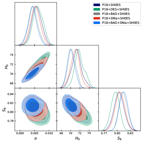
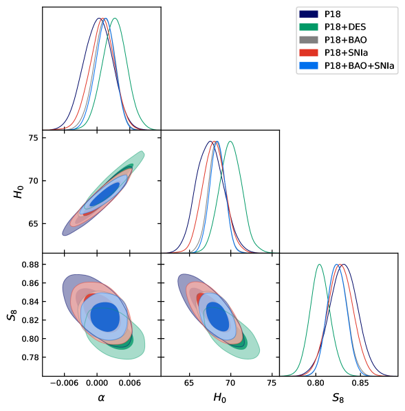
Figure 1: Confidence contours and posterior distributions for MI ($\alpha\neq 0$, $\Omega_{k}=0$): SH0ES prior included (top panel) or excluded (bottom panel).

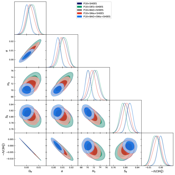
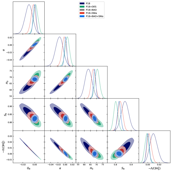
Figure 2: Confidence contours and posterior distributions for MII ($\alpha\neq 0$, $\Omega_{k}\neq 0$): SH0ES prior included (top panel) or excluded (bottom panel).

It is clear from figure 2 that including the SH0ES prior in the analysis, while assuming MII, results in a factor two upward boost of $\alpha$. However, the uncertainty correspondingly grows. These twice as large higher $\alpha$ values correspond to $\sim 2\%$ lower temperatures at $z\approx 1090$ than naively expected, i.e. recombination takes place at $z_{\star}\approx 1110$, earlier than expected based on the SM, $z_{\star}\approx 1089$. Recombination then takes place earlier than in MII, and consequently a higher $H_{0}$ value is deduced, in a better agreement with the SH0ES prior.

4 Summary

The $\gtrsim 5\sigma$ “Hubble tension” between the locally inferred Hubble constant (Cepheids and quasar lensing combined) and the value obtained from best-fit inference of cosmological parameters towards the last scattering surface, or other cosmological probes such as BAO, increasingly becomes a pressing issue faced by the SM of cosmology.

In the present work a cosmological model is proposed based on GR with extended (Weyl) symmetry. It is spherically-symmetric around any observer. The model explored here is described by a specific spherically symmetric metric of the “canonical” form out of infinitely many other possible spherically-symmetric metrics. While they can be always brought to this canonical form via an appropriate combination of coordinate and Weyl transformations, and null geodesics are blind to the latter, they are not indifferent to the former. Nevertheless, the particular model explored here already provides a better fit to cosmological data (with local $H_{0}$ constraints included) than does the SM, thereby providing a proof of principle to the idea that the Hubble tension could be significantly alleviated within this extended framework.

The scale factor in this model satisfies the Friedmann equation, exactly as it does in the SM. Whereas active gravitational masses and energy densities have radial dependencies, all contributions to the energy budget have the exact same spatial dependence; dimensionless (observables) ratios of energy densities of the various species are thus purely time-dependent and the cosmological principle is consequently respected. Similarly, ratios of number densities of any two species remain time-dependent only; although both the number densities of baryons, $n_{b}$, and photons, $n_{\gamma}\propto T^{3}$, are radially-dependent (from the perspective of any observer) in the proposed model, their ratio $\eta_{b}$ is purely time-dependent, and has its locally estimated value. Thus, the model is consistent with BBN to the extent that the SM is.

Based on the results shown in table 2 the most statistically favorable configuration, i.e. that makes the most dramatic improvement in fitting the data as compared to the SM, is achieved in the case that the SH0ES prior is imposed along with the assumption that space is globally flat where the DIC gain decisively favors MI over the SM. In that case we obtain that $(\gamma/H_{0})^{-1}\sim 100$, i.e. that the model fundamental length scale is O(100) times larger than the Hubble scale. This new parameter is different from zero at $\gtrsim 3\sigma$ confidence level and amounts to an equivalent $1.5\%$ lower $T_{CMB}$ at $z\approx 1089$ than extrapolated in a standard FRW model from the locally deduced value. For example, considering the P18+SH0ES data combination we obtain $z_{\star}=1089.53\pm 0.24$, $z_{\star}=1110.7^{+6.1}_{-7.0}$ & $z_{\star}=1105.4\pm 7.9$ in the SM, MI & MII, respectively, i.e. recombination takes place at higher redshifts (at 99 & 95% confidence level, respectively) than it does assuming the SM. This earlier-than-expected recombination implies higher $H_{0}\sim 71.4\pm 1.2$ & $72.2\pm 1.3$ km/sec/Mpc values, thereby significantly weakening currently estimated tension levels to $\sim 1.4$ & $1\sigma$ confidence levels, respectively.

The proposed model is dynamically equivalent to the SM but is kinematically different thanks to a new fundamental length scale $\gamma^{-1}$ and the different $K$-dependence. This may, at least partially, explain the Hubble tension and account for the anomalously negative curvature parameter deduced from the P18 data set. The latter is clearly seen from table 4 in case of P18 data alone; wheres assuming SM+K results in $\Omega_{k}=-0.0106^{+0.0069}_{-0.0059}$, MII is consistent with vanishing $\Omega_{k}$ and $\alpha=-0.016\pm 0.010$, only slightly reducing the Hubble tension from 4 to 3.4$\sigma$. The advantage is clear; while $\Omega_{k}\sim-0.01$ at present is finely tuned, $\alpha=-0.016$ at present is a comfortably natural value within the “allowed” range [-0.3, 0.3].

From a more fundamental standpoint, the present work highlights the tantalizing possibility that the CMB temperature generally evolves in the comoving frame in models described by metrics with space-dependent lapse functions. This provides a concrete realization of the idea that $T_{CMB}(z)$ could depart from its expected value based on local measurements of $T_{0}$ and assuming the FRW model, thereby alleviating the Hubble tension. More important, the Hubble tension might just be an indication that gravitation is genuinely Weyl invariant on macroscopic scales.

APPENDIX: WEYL INVARIANT SCALAR-TENSOR THEORY

In this Appendix we formulate the idea employed in this work, that gravitation is fundamentally endowed with WI, within a specific Weyl invariant scalar-tensor (WIST) framework, although as we emphasized above our results apply to any WI theory of gravitation that admits the FRW metric solution. WIST reduces to GR in a particular conformal frame.

GR is governed by the EH action

$$\mathcal{I}_{EH}=\int\left(R+\mathcal{L}_{M}\right)\sqrt{-g}d^{4}x,$$ (A1)

where we adopt units system in which $16\pi G=1$, and $\mathcal{L}_{M}$ is the lagrangian density associated with perfect fluid. In particular, any mass terms appearing in $\mathcal{L}_{M}$ are by definition active gravitational masses, which need not be equivalent to inertial or passive gravitational masses. While these three types of mass are not necessarily equivalent [82], the notion of a passive gravitational mass in any theory of gravity that satisfies the equivalence principle is vacuous. If the ratio of the later two mass types is a universal constant then the equivalence principle is satisfied – an assumption that we indeed make in the present work. The other three fundamental interactions are described by $\mathcal{L}_{SM}$, the lagrangian of the SM of particle physics where any mass is inertial, may it be generated via the Higgs mechanism in the electroweak sector or via the explicitly broken chiral symmetry in QCD.

Affecting the transformations $g_{\mu\nu}\rightarrow\frac{1}{6}\phi\phi^{*}g_{\mu\nu}$ and $\mathcal{L}_{M}\rightarrow 36\mathcal{L}_{M}/|\phi|^{4}$, where $\phi$ is a complex scalar field, in eq. (A1), leaves the latter invariant under local rescaling insofar $|\phi|^{2}g_{\mu\nu}$ is invariant, i.e.

$$\phi \rightarrow \phi/\Omega$$

$$g_{\mu\nu} \rightarrow \Omega^{2}g_{\mu\nu}$$

$$\mathcal{L}_{M} \rightarrow \mathcal{L}_{M}/\Omega^{4},$$ (A2)

where $\Omega(x)>0$ is a (arbitrary) well-behaved function of spacetime.

Since the curvature scalar depends on derivatives of the metric field it transforms inhomogeneously under Weyl transformations

$$R\rightarrow\Omega^{-2}\left(R-6\frac{\Box\Omega}{\Omega}\right),$$ (A3)

where $\Box$ is the d’Alambertian. WI of the first term in eq. (A1) would require that G is promoted to a dynamical scalar field. Combining this with eq. (A3), and integration by parts, results in the following WIST action of the Bergmann-Wagoner type [83, 84]

$$\mathcal{I}_{WIST}=\int\left(\frac{1}{6}|\phi|^{2}R+\phi^{*}_{\mu}\phi^{\mu}+\mathcal{L}_{M}(|\phi|)\right)\sqrt{-g}d^{4}x,$$ (A4)

where $\phi_{\mu}\equiv\phi_{,\mu}$, the matter lagrangian density $\mathcal{L}_{M}$ explicitly depends on the scalar field $\phi$, and the inhomogeneous term on the right hand side of eq. (A3) is compensated by a similar inhomogeneous term from the transformation of the kinetic term, $\phi^{*}_{\mu}\phi^{\mu}$. Eq. (A4) was first obtained by Deser [85] and later considered by, e.g. [86-96] with $\mathcal{L}_{M}$ not necessarily depending on $\phi$. Other aspects of the theory described by eq. (A4) have been recently explored in [97]. In [85] $\phi$ was assumed to be real. It can be easily shown via a simple field redefinition that eq. (A4) is equivalent to a Brans-Dicke (BD) theory with a BD parameter $\omega_{BD}=-3/2$ in the vacuum case. We emphasize that unlike in BD theory where the scalar field is only a replacement for the Planck mass, here the source term for the gravitational field, $\mathcal{L}_{M}$, explicitly depends on $|\phi|$, and all active gravitational masses and the Planck mass are thus proportional to the same scalar field, $\phi$. For example, and as will be clear below, the lagrangian density of non-relativistic (NR) matter and cosmological constant (CC) are $\mathcal{L}_{NR}\propto|\phi|$ and $\mathcal{L}_{CC}\propto|\phi|^{4}$, respectively. The lagrangian density of radiation is independent of $\phi$.

The field equations obtained from variation of eq. (A4) with respect to $g_{\mu\nu}$ and $\phi$ are, respectively,

$$\frac{|\phi|^{2}}{3}G_{\mu\nu} = T_{M,\mu\nu}+\Theta_{\mu\nu}$$ (A5)

$$\frac{1}{6}\phi R-\Box\phi+\frac{\partial\mathcal{L}_{M}}{\partial\phi^{*}} = 0,$$ (A6)

where

$$3\Theta_{\mu\nu}\equiv\phi^{*}_{\mu;\nu}\phi-2\phi^{*}_{\mu}\phi_{\nu}-g_{\mu\nu}(\phi^{*}\Box\phi-\frac{1}{2}\phi_{\alpha}^{*}\phi^{\alpha})+c.c.$$ (A7)

Here and throughout, $f_{\mu}^{\nu}\equiv(f_{,\mu})^{;\nu}$, and $(T_{M})_{\mu\nu}\equiv-\frac{2}{\sqrt{-g}}\frac{\delta(\sqrt{-g}\mathcal{L}_{M})}{\delta g^{\mu\nu}}$ is the energy-momentum tensor. Eq. (A5) is a generalization of Einstein equations with $\frac{|\phi|^{2}}{3}$ replacing $1/(16\pi G)$, and $\Theta_{\mu\nu}$ is an effective contribution to the energy momentum tensor essentially due to gradients of G and active gravitational masses. Multiplying eq. (A6) by $\phi^{*}$, combining with the its complex conjugate and the trace of eq. (A5), results in the constraint equation

$$\phi^{*}\frac{\partial\mathcal{L}_{M}}{\partial\phi^{*}}+\phi\frac{\partial\mathcal{L}_{M}}{\partial\phi}=T_{M},$$ (A8)

i.e. only pure radiation $T_{rad}=0$ is consistent with the theory described by eq. (A4) unless $\mathcal{L}_{M}$ explicitly depends on $|\phi|$. Recalling that $\mathcal{L}_{M}$ is a potential in $\phi$ it then follows that $\rho_{M}=\mathcal{L}_{M}$ and since for a perfect fluid with EOS $w_{M}$ the trace is $T_{M}=-\rho_{M}(1-3w_{M})$ it then follows from eq. (A8) that $\mathcal{L}_{M}\propto|\phi|^{1-3w_{M}}$, i.e it is linear and quartic in $|\phi|$ in cases of NR and vacuum-like matter respectively, and is independent of $|\phi|$ in case of pure radiation. Linearity of $\mathcal{L}_{M}$ in $|\phi|$ in the case vanishing EOS, $w_{M}=0$, suggests that active gravitational masses are regulated by $|\phi|$. Not only that the same $\phi$ determining both Planck mass and active gravitational masses is necessary for the consistency of non-radiation sources with this WI theory, it is also a conceptually natural “conclusion” as the concept of active gravitational mass is meaningless unless it couples to G, and in this sense it seems natural that both quantities are determined by the same scalar field. This clearly does not have necessarily to be the case in general (as in e.g, BD theory), but it is a nice merit of the model, and actually mandatory in case of the WI theory described by eq. (A4).

Within this formalism, the proposed cosmological model is obtained from the SM via a combined coordinate and conformal transformations which are given by eq. (4), $\Omega^{2}=(r/r^{\prime})^{2}=1+\gamma r-\frac{\Lambda}{3}r^{2}$. Consequently, $m_{pl}\rightarrow m_{pl}(1+\gamma r-\frac{\Lambda}{3}r^{2})^{-1/2}$, and $m_{pl}$ in the new frame, eq. (2), is now r-dependent as measured by any observer. As mentioned below eq. (4), the metric describing our model has a divergent curvature $R=-12(K+\frac{\gamma^{2}}{4})-\frac{6\gamma}{r}$. This divergence does not go away even if we consider the dimensionless combination $R/|\phi|^{2}$. However, Weyl invariant quantities must have a vanishing conformal weight by definition. Such a zero conformal weight combination involving $R$ is, e.g.

$$\frac{-|\phi|^{2}R+6{\rm Re}(\phi\Box\phi^{*})}{|\phi|^{4}}=\frac{3T_{M}}{|\phi|^{4}}.$$ (A9)

Since $\frac{T_{M}}{|\phi|^{4}}$ is invariant under conformal transformation, and is $\propto\rho_{M}(\eta)$ in the SM, it is clear that it is purely time dependent, and the divergence of $R$ at $r=0$ automatically vanishes. The latter is canceled by a similar divergence of the $\phi\Box\phi^{*}$ term, i.e. gradients of the scalar field (i.e. $G$ or equivalently $m_{pl}$, and $M_{act}$).

References

- [1] P. Vielva, E. Martínez-González, R. B. Barreiro et al., ‘Detection of Non-Gaussianity in the Wilkinson Microwave Anisotropy Probe First-Year Data Using Spherical Wavelets’, Astrophys. J. 609 (2004) 22 [astro-ph/0310273]
- [2] A. Wiegand, T. Buchert and M. Ostermann, ‘Direct Minkowski Functional analysis of large redshift surveys: a new high-speed code tested on the luminous red galaxy Sloan Digital Sky Survey-DR7 catalogue’, Mon. Not. R. Astron. Soc. 443 (2014) 241 [arXiv:1311.3661]
- [3] R. A. Battye, T. Charnock and A. Moss, ‘Tension between the power spectrum of density perturbations measured on large and small scales’, Phys. Rev. D 91 (2015) 103508 [arXiv:1409.2769]
- [4] N. MacCrann, J. Zuntz, S. Bridle, et al, ‘Cosmic discordance: are Planck CMB and CFHTLenS weak lensing measurements out of tune?’, Mon. Not. R. Astron. Soc. 451 (2015) 2877 [arXiv:1408.4742]
- [5] T. Delubac, J. E. Bautista, N. G. Busca, et al, ‘Baryon acoustic oscillations in the Ly forest of BOSS DR11 quasars’, Astron. Astrophys. 574 (2015) A59 [1404.1801]
- [6] P. Bull, Y. Akrami, J. Adamek, et al., ‘Beyond CDM: Problems, solutions, and the road ahead’, Physics of the Dark Universe 12 (2016) 56 [arXiv:1512.05356]
- [7] S. Nesseris, G. Pantazis and L. Perivolaropoulos, ‘Tension and constraints on modified gravity parametrizations of (z) from growth rate and Planck data’, Phys. Rev. D 96 (2017) 023542 [arXiv:1703.10538]
- [8] S. Vagnozzi, A. Loeb and M. Moresco, ‘Eppur è piatto? The Cosmic Chronometers Take on Spatial Curvature and Cosmic Concordance’, Astrophys. J. 908 (2021) 64 [arXiv:2011.11645]
- [9] Planck Collaboration, N. Aghanim, Y. Akrami, et al, ‘Planck 2018 results. VI. Cosmological parameters’, Astron. Astrophys. 641 (2020) A6 [arXiv:1807.06209]
- [10] S. Aiola, E. Calabrese, L. Maurin, et al., ‘The Atacama Cosmology Telescope: DR4 maps and cosmological parameters’, JCAP 2020 (2020) 047 [arXiv:2007.07288]
- [11] M. M. Ivanov, M. Simonović and M. Zaldarriaga, ‘Cosmological parameters from the BOSS galaxy power spectrum’, JCAP 2020 (2020) 042 [arXiv:1909.05277]
- [12] W. L. Freedman, ‘Correction: Cosmology at a crossroads’, Nat. Astron. 1 (2017) 0169 [arXiv:1706.02739]
- [13] A. G. Riess, S. Casertano, W. Yuan, et al., ‘Milky Way Cepheid Standards for Measuring Cosmic Distances and Application to Gaia DR2: Implications for the Hubble Constant’, Astrophys. J. 861 (2018) 126 [arXiv:1804.10655]
- [14] A. G. Riess, S. Casertano, W. Yuan, et al., ‘Large Magellanic Cloud Cepheid Standards Provide a 1% Foundation for the Determination of the Hubble Constant and Stronger Evidence for Physics beyond CDM’, Astrophys. J. 876 (2019) 85 [arXiv:1903.07603]
- [15] S. Birrer, T. Treu, C. E. Rusu et al., ‘H0LiCOW - IX. Cosmographic analysis of the doubly imaged quasar SDSS 1206+4332 and a new measurement of the Hubble constant’, Mon. Not. R. Astron. Soc. 484 (2019) 4726 [arXiv:1809.01274]
- [16] K. C. Wong, S. H. Suyu, G. C.-F. Chen, et al., ‘H0LiCOW – XIII. A 2.4 per cent measurement of from lensed quasars: 5.3 tension between early- and late-Universe probes’, Mon. Not. R. Astron. Soc. 498 (2020) 1420 [arXiv:1907.04869]
- [17] A. J. Shajib, S. Birrer, T. Treu, et al., ‘STRIDES: a 3.9 per cent measurement of the Hubble constant from the strong lens system DES J0408-5354’, Mon. Not. R. Astron. Soc. 494 (2020) 6072 [arXiv:1910.06306]
- [18] D. W. Pesce, J. A. Braatz, M. J. Reid, et al., ‘The Megamaser Cosmology Project. XIII. Combined Hubble Constant Constraints’, Astrophys. J. Lett 891 (2020) L1 [arXiv:2001.09213]
- [19] J. Schombert, S. McGaugh and F. Lelli, ‘Using the Baryonic Tully-Fisher Relation to Measure ’, Astron. J. 160 (2020) 71 [arXiv:2006.08615]
- [20] T. de Jaeger, B. E. Stahl, W. Zheng, et al., ‘A measurement of the Hubble constant from Type II supernovae’, Mon. Not. R. Astron. Soc. 496 (2020) 3402 [arXiv:2006.03412]
- [21] W. L. Freedman, B. F. Madore, D. Hatt et al., ‘The Carnegie-Chicago Hubble Program. VIII. An Independent Determination of the Hubble Constant Based on the Tip of the Red Giant Branch’, Astrophys. J. 882 (2019) 34 [arXiv:1907.05922]
- [22] W. L. Freedman, ‘Measurements of the Hubble Constant: Tensions in Perspective’ ApJ 919 (2021) 16 [arXiv:2106.15656]
- [23] W. Yuan, A. G. Riess, L. M. Macri, et al., ‘Consistent Calibration of the Tip of the Red Giant Branch in the Large Magellanic Cloud on the Hubble Space Telescope Photometric System and a Redetermination of the Hubble Constant’, Astrophys. J. 886 (2019) 61 [arXiv:1908.00993]
- [24] W. L. Freedman, B. F. Madore, T. Hoyt, et al., ‘Calibration of the Tip of the Red Giant Branch’, Astrophys. J. 891 (2020) 57 [arXiv:2002.01550]
- [25] M. Rameez & S. Sarkar, ‘Is there really a Hubble tension?’ CQG 38 (2021) 154005 [arXiv:1911.06456]
- [26] C. L. Bennett, D. Larson, J. L. Weiland, et al., ‘The 1% Concordance Hubble Constant’, Astrophys. J. 794 (2014) 135 [arXiv:1406.1718]
- [27] Y. Wang, L. Xu and G.-B. Zhao, ‘A Measurement of the Hubble Constant Using Galaxy Redshift Surveys’, Astrophys. J. 849 (2017) 84 [arXiv:1706.09149]
- [28] H.-Y. Chen, M. Fishbach and D. E. Holz, ‘A two per cent Hubble constant measurement from standard sirens within five years’, Nature 562 (2018) 545 [arXiv:1712.06531]
- [29] S. M. Feeney, H. V. Peiris, A. R. Williamson, et al., ‘Prospects for Resolving the Hubble Constant Tension with Standard Sirens’, Phys. Rev. Lett. 122 (2019) 061105 [arXiv:1802.03404]
- [30] K. Hotokezaka, E. Nakar, O. Gottlieb, et al., ‘A Hubble constant measurement from superluminal motion of the jet in GW170817’, Nat. Astron. 3 (2019) 940 [arXiv:1806.10596]
- [31] D. J. Mortlock, S. M. Feeney, H. V. Peiris, et al., ‘Unbiased Hubble constant estimation from binary neutron star mergers’, Phys. Rev. D 100 (2019) 103523 [arXiv:1811.11723]
- [32] J. Hamann and J. Hasenkamp, ‘A new life for sterile neutrinos: resolving inconsistencies using hot dark matter’, JCAP 2013 (2013) 044 [arXiv:1308.3255]
- [33] R. A Battye and A. Moss, ‘Evidence for Massive Neutrinos from Cosmic Microwave Background and Lensing Observations’, Phys. Rev. Lett. 112 (2014) 051303 [arXiv:1308.5870]
- [34] C. Dvorkin, M. Wyman, D. H. Rudd, et al., ‘Neutrinos help reconcile Planck measurements with both the early and local Universe’, Phys. Rev. D 90 (2014) 083503 [arXiv:1403.8049]
- [35] M. Wyman, D. H. Rudd, R. A. Vanderveld, et al., ‘Neutrinos Help Reconcile Planck Measurements with the Local Universe’, Phys. Rev. Lett. 112 (2014) 051302 [arXiv:1307.7715]
- [36] E. Di Valentino, A. Melchiorri and J. Silk, ‘Reconciling Planck with the local value of in extended parameter space’, Phys. Lett. B 761 (2016) 242 [arXiv:1606.00634]
- [37] E. Di Valentino, A. Melchiorri and O. Mena, ‘Can interacting dark energy solve the tension?’, Phys. Rev. D 96 (2017) 043503 [arXiv:1704.08342]
- [38] E. Di Valentino, ‘Crack in the cosmological paradigm’, Nat. Astron. 1 (2017) 569 [arXiv:1709.04046]
- [39] E. Di Valentino, C. Bœhm, E. Hivon, et al., ‘Reducing the and tensions with dark matter-neutrino interactions’, Phys. Rev. D 97 (2018) 043513 [arXiv:1710.02559]
- [40] E. Di Valentino, E. V. Linder and A. Melchiorri, ‘Vacuum phase transition solves the tension’, Phys. Rev. D 97 (2018) 043528 [arXiv:1710.02153]
- [41] F. D’Eramo, R. Z. Ferreira, A. Notari, et al., ‘Hot axions and the tension’, JCAP 2018 (2018) 014 [arXiv:1808.07430]
- [42] V. Poulin, T. L. Smith, T. Karwal, et al., ‘Early Dark Energy can Resolve the Hubble Tension’, Phys. Rev. Lett. 122 (2019) 221301 [arXiv:1811.04083]
- [43] K. Vattis, S. M. Koushiappas and A. Loeb, ‘Dark matter decaying in the late Universe can relieve the tension’, Phys. Rev. D 99 (2019) 121302 [arXiv:1903.06220]
- [44] C. D. Kreisch, F.-Y. Cyr-Racine and O. Doré, ‘Neutrino puzzle: Anomalies, interactions, and cosmological tensions’, Phys. Rev. D 101 (2020) 123505 [arXiv:1902.00534]
- [45] K. L. Pandey, T. Karwal and S. Das, ‘Alleviating the and anomalies with a decaying dark matter model’, JCAP 2020 (2020) 026 [arXiv:1902.10636]
- [46] E. Di Valentino, A. Melchiorri, O. Mena, et al., ‘Nonminimal dark sector physics and cosmological tensions’, Phys. Rev. D, 101 (2020) 063502 [arXiv:1910.09853]
- [47] S. Vagnozzi, ‘New physics in light of the H0 tension: An alternative view’, Phys. Rev. D 102 (2020) 023518 [arXiv:1907.07569]
- [48] T. L. Smith, V. Poulin and M. A Amin, ‘Oscillating scalar fields and the Hubble tension: A resolution with novel signatures’, Phys. Rev. D 101 (2020) 063523 [arXiv:1908.06995]
- [49] E. Di Valentino, L. A. Anchordoqui, O. Akarsu, et al., ‘Cosmology Intertwined II: The Hubble Constant Tension’, 2020 [arXiv:2008.11284]
- [50] E. Di Valentino, O. Mena, S. Pan, et al., ‘In the Realm of the Hubble tension – a Review of Solutions’, (2021) [arXiv:2103.01183]
- [51] P. Shah, P. Lemos, & O. Lahav, ‘A buyer’s guide to the Hubble Constant’ (2021) [arXiv:2109.01161]
- [52] S. L. Bridle, A. M. Lewis, J. Weller, et al., ‘Reconstructing the primordial power spectrum’, Mon. Not. R. Astron. Soc. 342 (2003) L72 [astro-ph/0302306]
- [53] C. R. Contaldi, M. Peloso, L. Kofman, et al., ‘Suppressing the lower multipoles in the CMB anisotropies’, JCAP 2003 (2003) 002 [astro-ph/0303636]
- [54] A. Iqbal, J. Prasad, T. Souradeep, et al., ‘Joint Planck and WMAP assessment of low CMB multipoles’, JCAP 2015 (2015) 014 [arXiv:1501.02647]
- [55] M. Shimon, ‘Weyl-invariant gravity and the nature of dark matter’, Class. Quantum Gravity 38 (2021) 085001 [arXiv:2012.04472]
- [56] M. M. Ivanov, Y. Ali-Haïmoud and J. Lesgourgues, ‘ tension or tension?’, Phys. Rev. D 102 (2020) 063515 [arXiv:2005.10656]
- [57] B. Bose & L. Lombriser, ‘Easing cosmic tensions with an open and hotter universe’, Phys. Rev. D 103 (2021) L081304 [arXiv:2006.16149]
- [58] M. Shimon and Y. Rephaeli, ‘Parameter interplay of CMB temperature, space curvature, and expansion rate’, Phys. Rev. D 102 (2020) 083532 [arXiv:2009.14417]
- [59] Y. Wen, D. Scott, R. Sullivan, et al. 2020, ‘The role of in CMB anisotropy measurements’, Phys. Rev. D 104 (2021) 043516 [arXiv:2011.09616]
- [60] C. Bonvin and P. Fleury, ‘Testing the equivalence principle on cosmological scales’, JCAP 2018 (2018) 061 [arXiv:1803.02771]
- [61] W. de Sitter, it ‘Einstein’s theory of gravitation and its astronomical consequences. Third paper’, Mon. Not. R. Astron. Soc. 78 (1917) 3
- [62] W. de Sitter, ‘On the curvature of space’, Koninklijke Nederlandse Akademie van Wetenschappen Proceedings Series B Physical Sciences 20 (1918) 229
- [63] A. S. Eddington, The mathematical theory of relativity, by A.S. Eddington. Cambridge: University Press, 1923, 1st edition
- [64] R. C. Tolman, ‘On the Astronomical Implications of the de Sitter Line Element for the Universe’, Astrophys. J. 69 (1929) 245
- [65] G. Stromberg, ‘Analysis of radial velocities of globular clusters and non-galactic nebulae’, Astrophys. J. 61 (1925) 353
- [66] D. J. Fixsen, ‘The Temperature of the Cosmic Microwave Background’, Astrophys. J. 707 (2009) 916 [arXiv:0911.1955]
- [67] P. D. Mannheim and D. Kazanas, ‘Exact Vacuum Solution to Conformal Weyl Gravity and Galactic Rotation Curves’, Astrophys. J. 342 (1989) 635
- [68] P. D. Mannheim and J. G. O’Brien, ‘Impact of a Global Quadratic Potential on Galactic Rotation Curves’, Phys. Rev. Lett. 106 (2011) 121101 [arXiv:1007.0970]
- [69] P. D. Mannheim and J. G. O’Brien, ‘Fitting galactic rotation curves with conformal gravity and a global quadratic potential’, Phys. Rev. D 85 (2012) 124020 [arXiv:1011.3495]
- [70] J. G O’Brien and P. D. Mannheim, ‘Fitting dwarf galaxy rotation curves with conformal gravity’, Mon. Not. R. Astron. Soc. 421 (2012) 1273 [arXiv:1107.5229]
- [71] Efstathiou G 2020 [arXiv:2007.10716]
- [72] A. Gelman and D. B. Rubin, ‘Inference from Iterative Simulation Using Multiple Sequences’, Statist. Sci. 7 (1992) 457
- [73] A. R Liddle, ‘Information criteria for astrophysical model selection’, Mon. Not. R. Astron. Soc. 377 (2007) L74 [astro-ph/0701113]
- [74] R. Trotta, ‘Bayes in the sky: Bayesian inference and model selection in cosmology’, Contemp. Phys. 49 (2008) 71 [arXiv:0803.4089]
- [75] X. Xu, A. J. Cuesta, N. Padmanabhan, et al., ‘Measuring DA and H at z=0.35 from the SDSS DR7 LRGs using baryon acoustic oscillations’, Mon. Not. R. Astron. Soc. 431 (2013) 2834 [arXiv:1206.6732]
- [76] É Aubourg, S. Bailey, J. E. Bautista, et al., ‘Cosmological implications of baryon acoustic oscillation measurements’, Phys. Rev. D 92 (2015) 123516 [arXiv:1411.1074]
- [77] J. L. Bernal, T. L. Smith, K. K. Boddy, et al., ‘Robustness of baryon acoustic oscillation constraints for early-Universe modifications of CDM cosmology’, Phys. Rev. D 102 (2020) 123515 [arXiv:2004.07263]
- [78] G. d’Amico, J. Gleyzes, N. Kokron, et al., ‘The Cosmological Analysis of the SDSS/BOSS data from the Effective Field Theory of Large-Scale Structure’, JCAP 2020 (2020) 005 [arXiv:1909.05271]
- [79] T. Colas, G. d’Amico, L. Senatore, et al., ‘Efficient Cosmological Analysis of the SDSS/BOSS data from the Effective Field Theory of Large-Scale Structure’ JCAP 2020 (2020) 001 [arXiv:1909.07951]
- [80] E. Di Valentino, A. Melchiorri and J. Silk, ‘Planck evidence for a closed Universe and a possible crisis for cosmology’, Nat. Astron. 4 (2020) 196 [arXiv:1911.02087]
- [81] W. Handley, ‘Curvature tension: evidence for a closed universe’, Phys. Rev. D 103 (2019) 041301 [arXiv:1908.09139]
- [82] H. Bondi, ‘Negative Mass in General Relativity’, Rev. Mod. Phys., 29 (1957) 423
- [83] P. G. Bergmann, ‘Comments on the scalar-tensor theory’, Int. J. Theor. Phys. 1 (1968) 25
- [84] R. V. Wagoner, ‘Scalar-Tensor Theory and Gravitational Waves’, Phys. Rev. D 1 (1970) 3209
- [85] S. Deser, ‘Scale invariance and gravitational coupling’, Ann. Phys. 59 (1970) 248
- [86] J. L. Anderson, ‘Scale Invariance of the Second Kind and the Brans-Dicke Scalar-Tensor Theory’, Phys. Rev. D 3 (1971) 1689
- [87] P. G. O. Freund, ‘Local scale invarlance and gravitation’, Annals of Physics 84 (1974) 440
- [88] R. Kallosh, ‘On the renormalization problem of quantum gravity’, Physics Letters B 55, (1975) 321
- [89] F. Englert, E. Gunzig, C. Truffin, et al., ‘Conformal invariant general relativity with dynamical symmetry breakdown’, Phys. Lett. B 57 (1975) 73
- [90] L. Smolin, ‘Gravitational radiative corrections as the origin of spontaneous symmetry breaking!’, Phys. Lett. B, 93 (1980) 95
- [91] T. Padmanabhan, ‘LETTER TO THE EDITOR: Conformal invariance, gravity and massive gauge theories’, Class. Quantum Gravity 2 (1985) L105
- [92] ’t Hooft, ‘A Class of Elementary Particle Models Without Any Adjustable Real Parameters’, Foundations of Physics 41 (2011) 1829 [arXiv:1104.4543]
- [93] A. Edery, L. Fabbri & M. B. Paranjape, ‘Spontaneous breaking of conformal invariance in theories of conformally coupled matter and Weyl gravity’, Class. Quantum Gravity 23 (2006) 6409 [hep-th/0603131]
- [94] I. Bars, S.-H. Chen, P. J. Steinhardt, et al., ‘Antigravity and the big crunch/big bang transition’ Phys. Lett. B 715 (2012) 278 [arXiv:1112.2470]
- [95] I. Bars, S.-H. Chen, P. J. Steinhardt, et al., ‘Complete set of homogeneous isotropic analytic solutions in scalar-tensor cosmology with radiation and curvature’, Phys. Rev. D 86 (2012) 083542 [arXiv:1207.1940]
- [96] R. Kallosh & A. Linde, ‘Universality class in conformal inflation’, JCAP 2013 (2013) 002 [arXiv:1306.5220]
- [97] M. Shimon (2021), ‘Weyl-invariant gravity’, arXiv:2108.11788