Geometric Scene Refocusing

Abstract

An image captured with a wide-aperture camera exhibits a finite depth-of-field, with focused and defocused pixels. A compact and robust representation of focus and defocus helps analyze and manipulate such images. In this work, we study the fine characteristics of images with a shallow depth-of-field in the context of focal stacks. We present a composite measure for focus that is a combination of existing measures. We identify in-focus pixels, dual-focus pixels, pixels that exhibit bokeh and spatially-varying blur kernels between focal slices. We use these to build a novel representation that facilitates easy manipulation of focal stacks. We present a comprehensive algorithm for post-capture refocusing in a geometrically correct manner. Our approach can refocus the scene at high fidelity while preserving fine aspects of focus and defocus blur.

I Introduction

Sharp and soft focus are important attributes of a good photograph. Focus and defocus blur are used creatively by photographers to produce remarkable compositional effects. An image captured using a wide-aperture camera is a collection of differently focused scene points. Cameras with a wide aperture are available on devices ranging from high-end mobile phones to DLSRs. The relative geometry of the sensor and the lens at capture-time governs the points in the scene that appear focused in the image. Light arriving from these focused points contributes to a single or very few pixels on the sensor. Other regions of the scene appear defocused by an amount proportionate to their distance from the in-focus region. The luminosity of defocused scene points is distributed across a set of proximate pixels, and this spread is referred to as a defocus kernel. The size and shape of this kernel depends on the distance of the scene point from the in-focus region and its 2-dimensional pixel location in the image. Defocus kernels of proximate pixels may overlap with each other, leading to complex pixel interactions. An accurate model of focus and defocus blur is relevant to computational photography as it can enable measurement of focus for tasks such as de-blurring, depth-of-field extension, refocusing and depth-from-focus. Post-capture modeling of focus and defocus blur using only a single image is an ill-constrained problem. Accurate focus modeling usually requires multi-focus imagery and a robust method to estimate in-focus pixels and defocus kernels.

In-focus pixels can be estimated by measuring the sharpness across each pixel’s neighborhood. In-focus pixels are expected to be sharp while defocused pixels exhibit low contrast. However, sharpness alone is an unreliable estimate as it is dependent on the texture and arrangement of scene points. Furthermore, the intensity of a pixel is quantized by the dynamic range of the sensor and may not represent the original luminosity of its scene point. The intensity might also be mixed with the defocused intensity of other scene points. These issues complicate the task of identifying whether a pixel is in focus and by what amount.

Modeling the defocus kernel at a pixel is also a challenging task. The size and shape of a defocus kernel depends on the camera and scene geometry. The kernel shape is also affected by vignetting or kernel-shortening close to the boundaries of the aperture. The defocus spread from a farther scene point may be partially occluded by the presence of closer objects. Such interaction between defocus kernels from different depths requires accurate geometric modeling. In this work, we propose a robust method to estimate and manipulate focus and defocus blur. The main contributions of this work are:

1. We identify a composite measure of focus that combines the strengths of existing focus measures for estimating the true intensity and in-focus location(s) for each pixel.

2. We build a compact representation for multi-focus input imagery using the composite measure and a calibration method that estimates the size and shape of defocus kernels.

3. We propose a novel algorithm for geometric depth-of-field manipulation. Our algorithm correctly accounts for complex pixel interactions at depth edges using an occlusion coefficient.

Ours is a comprehensive study of focus and defocus and is applicable to variety of scenes captured as a focal stack. Careful analysis of focus and defocus blur along with simple models that help in synthesis are the primary strengths of this work. We expect our model to be used by image editing tools in conjunction with focal stacks or RGBD images to allow easy and quick post-capture manipulation of focus.

II Related Work

Focus and defocus blur have been widely studied in computer vision in the past, primarily in the context of image de-blurring to create an in-focus image of the scene. Since it is difficult to estimate the per-pixel focus profile from a single image, two or more images of the scene with different focus positions are typically used to measure focus and defocus blur. Focus variations in an image also provide implicit cues to estimate scene depth. We broadly discuss the contemporary work in computational photography that deals with wide-aperture images.

Epsilon Focus Photography - Focal Stacks

A focal stack is a collection of multiple wide-aperture images with a small change in the focus position between consequent shots. Focal stacks enable dense modeling of the focus profile for each pixel. These focus profiles are useful for tasks such as de-blurring, refocusing and depth estimation. Hasinoff et al. [1, 2, 3] show that focal stacks require a significantly less time to capture and exhibit reduced noise characteristics compared to a single image capturing the full depth-of-field. This however leads to a loss of temporal resolution due to the finite amount of time taken to capture each slice. Focal stacks are thereby limited to mostly static scenes, as moving objects complicate pixel-alignment across focal slices. Moreover, storing a full focal stack on the device can lead to large storage overheads on portable devices. Our previous work [4] illustrates a compact representation for a focal stack that enables basic post-capture focus control. In this work, we propose a representation that can reduce the storage complexity while also encoding the fine characteristics of each focal slice.

In-Focus Imaging

Estimating the in-focus scene content from focal slices is the primary application of focal stacks. An in-focus image of the scene is free of any ambiguity caused by defocus blur for tasks such as segmentation, recognition and retrieval. Kubota et al. [5] generate in-focus images using linear filtering of focal slices using a focal-texture model. Kodama and Kubota [6] extend this to a 3D filtering method for generating dense pin-hole views from novel viewpoints. Iterative computation of focal textures has also be used in our previous work to produce in-focus images for shallow focal stacks [7]. Nagahara et al. [8] use a special camera to capture a focal sweep of the scene by aggregating the light on the sensor during relative translation between the sensor and the lens. Deconvolution of the blurred focal sweep image yields an all-in-focus image. Kuthirummal et al. [9] use the same principle and average the captured focal slices to generate the integrated image from a focal stack. Agarwala et al. [10] generate an in-focus image from a focal stack using a global contrast maximization approach. In this work, we comprehensively identify the in-focus scene content for all pixels, including pixels that might exhibit multiple in-focus locations. This occurs at pixels from background segments that might be partially occluded by the foreground. We also locate the intensity saturated regions in the scene and approximately estimate the in-focus intensity for these scene points.

Measuring Focus

A focus measure is at the heart of any approach that uses wide-aperture images. Estimating whether a pixel is in focus or not requires a suitable focus measure. Measures of focus based on several image properties have been proposed in computer vision literature [11, 12, 13, 14, 15]. The response of a focus measure not only depends on the parameters of the measure but also on the textural content around the pixel in the image. Measuring per-pixel focus based solely on a single pixel’s response is usually noisy and unreliable [16]. Smooth focus maps that consider neighborhood consistency can be generated using optimization methods such as Cost-Volume Filtering [17] or MRF labeling [18]. Iterative optimization methods can also be used to estimate smooth focus maps [7, 19]. Pertuz et al. [20] analyze and compare several focus measures independently for the task of depth-from-focus. They conclude that Laplacian based operators are best suited under normal imaging conditions. In [21], the Laplacian focus measure is used to compare classical DfF energy minimization with a variational model. A Ring Difference Filter measure is proposed in [22], with a filter shape designed to encode the sharpness around a pixel using both local and non-local terms. Mahmood et al. [23] combine three well known focus measures (Tenengrad, Variance and Laplacian Energy) in a genetic programming framework. Boshtayeva et al. [24] describe the benefit of using multiple focus measures together in an anisotropic smoothing framework to compute scene depth. Measuring the focus information of a scene is in fact analogous to computing relative scene depth from multiple focused images [11, 25, 26, 27, 28, 29]. In this work, we learn a composite measure of focus as a weighted combination of several informative measures, building on our previous work on depth-from-focus [30].

PSF Modeling and Estimation

Modeling the spatially varying defocus kernel in wide-aperture images is relevant in the context of image de-blurring and scene refocusing. Kee et al. [31] remove spatially varying optical blur by estimating dense non-parametric blur kernels across the image. They describe calibration and kernel fitting methods for blur estimation. Shih et al. [32] show a calibration technique to predict the lens point-spread-function (PSF) at arbitrary depths using a calibrated PSF at a known depth. Tang and Kutulakos [33] describe an analytical approach for blind image de-blurring and PSF calibration at other pixels from known PSFs at some pixels. Hach et al. [34] show a dense calibration method for a high quality lens with depth-aware rendering to produce synthetic bokeh. In this work, we present a simple calibration method that estimates the size and shape of defocus kernels using the estimated in-focus pixels. We also identify the blur kernels at intensity saturated scene regions and render them appropriately while refocusing.

Flexible Depth-of-Field Imaging

Changing the focus position or the depth-of-field of an image after it has been captured is a useful tool in photography. Nagahara et al. [8] demonstrate flexible DoF effects by capturing disjoint focal sweeps through the scene and deconvolving the aggregate image by the integration kernel. Half-sweep imaging [35] has also been used on the same lines. Jacobs et al. [36] describe a precise composition model to generate composite images from the available focal slices using a defocus map that specifies the amount of target defocus at each pixel. They use geometric integration of rays for free-form depth-of-field control. The Lytro lightfield camera [37, 38] enables post-capture refocusing and interpolation by capturing a 4D lightfield at a limited resolution. In this work, we present a geometric approach for post-capture focus manipulation.

In a related parallel effort, we have used data-driven methods for post-capture focus control. In [39], we propose an adversarial learning framework trained on focal stacks created from light-fields to refocus the scene after it has been captured. The task of refocusing is decomposed into disjoint operations of de-blurring and re-blurring. We also propose an adversarial learning framework for defocus magnification [40]. Data driven methods for focus control have only recently gained popularity. Wang et al. [41] achieve post-capture control of depth-of-field by estimating the depth map using a convolutional neural network trained over a large RGBD dataset. Re-blurring the image to a target depth-of-field is also learned in a data-driven manner, with separate stream for image features and blur kernels. Data-driven methods suffer from a serious lack of generalizability in our experience. These methods may be able to capture the fine characteristics of wide aperture images, but will require large amounts of specific data to be able to do so effectively. In this work, we propose a geometric refocusing algorithm that can perform flexible DoF manipulation on any scene using multi-focus input imagery.

III Wide-Aperture Imaging

An image captured through a finite aperture opening consists of a combination of focused and defocused scene points. Unlike a pinhole camera that captures one (or very few) rays at each pixel, a wide aperture camera records the combination of several rays at a pixel. If the rays at a pixel arrive from the same scene point, the point manifests as an in-focus pixel in the image, while it appears as a defocused pixel if multiple scene points contribute to it as illustrated in Figure 1.

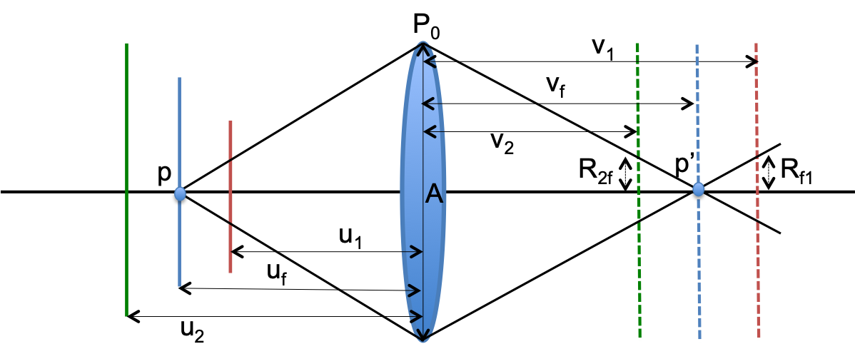
Figure 1: The rays from scene point $p$ at a depth $u_{f}$ converge at an in-focus pixel $p^{\prime}$ when the sensor is positioned at $v_{f}$. At other sensor positions such as $v_{1}$ and $v_{2}$, the rays from $p$ spread across a defocus kernel of radius $R_{f1}$ and $R_{2f}$ respectively.

The characteristics of a wide-aperture image such as field-of-view, depth-of-field, focus distance, amount of defocus at each pixel, image brightness and sensitivity depend on the nature of the lens and the capture-time camera parameters. Image formation in wide-aperture cameras is typically modeled as a two stage process. The first stage deals with the optical traversal of light through the lens assembly and its collection onto the discrete photo-electric sensor. The second stage consists of the conversion of sensor voltages to discrete pixel intensities in the image [42].

Modeling the image formation pipeline in wide-aperture cameras is important for accurate estimation and processing of focus and defocus blur. In this work, we identify crucial capture parameters such as in-focus pixels, dual focus pixels, defocus radii and intensity saturation from multiple wide-aperture images captured as an ordered focal stack.

A focal stack $\cal G$ is a sequence of $k$ images (called focal slices) ${\cal G}_{i},1\leq i\leq k$. Each slice is captured with a progressively varying focal distance but the same aperture opening. A focal slice ${\cal G}_{i}$ is the wide-aperture image corresponding to the focus position $i$ and can be defined as:

$${\cal G}_{i}=\int\int h^{i}(x,y,d_{(x,y)})\hat{{\cal G}}_{r}(x,y)\,dx\,dy\,,$$ (1)

where $h^{i}$ is a spatially varying defocus kernel whose size and shape depends on the spatial location of the pixel and the depth $d_{(x,y)}$ of its corresponding scene point and $\hat{{\cal G}}_{r}$ is the radiance or luminosity of the scene point. An ideal focal stack captures each scene point in sharp focus in one and only one focal slice. Focal slices exhibit magnification differences as the focus position varies. This can be corrected using image registration or image alignment. Once registered, a focal stack is a volume of pixels, with each node in the volume representing the pixel’s intensity in the corresponding slice. The variation of pixel intensities across this volume can be used to estimate in-focus scene points and defocus kernels as demonstrated in the forthcoming sections.

IV Measuring Focus

The sharpness of the image content across the two-dimensional neighborhood of a pixel is a reliable indicator of its amount of focus. Identifying the appropriate measure of sharpness in a scene independent manner is non-trivial. Figure 2 shows the response of different measures of focus/sharpness at two pixels in a focal stack. It can be seen that although these measures encode the sharpness around a pixel, they exhibit remarkable variability. A key contribution of our work is a composite focus measure (cFM) as a weighted combination of existing measures.

We study the performance of 39 focus measures - all measures from Pertuz et al. [20], two additional measures from Boshtayeva et al. [24] and the Ring Difference Filter from [22] - in the context of per-pixel focus estimation over a large dataset of focal stacks. We represent the focus measures using a similar convention to [20]; the additional measures are labeled as HFN (Frobenius Norm of the Hessian), DST (Determinant of Structure Tensor) and RDF (Ring Difference Filter). We compute focus profiles shown in Figure 2 for all the pixels in our focal stack dataset across all focus measures. We seek to select the best subset of focus measures using these focus profiles. A supervised approach to focus measure selection is not possible as ground-truth focus maps of the scene are not available. Unsupervised feature selection is thereby the natural choice for identifying a composite focus measure.

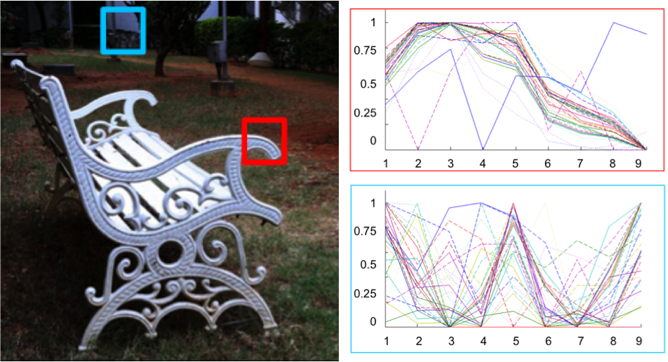
Figure 2: The focus profiles of thirty different focus measures evaluated at two pixels across a focal stack. Severe variability in in-focus estimation across different measures can observed based on the textural content around challenging pixels.

At each pixel, the agreement of different focus measures about the peak location of focus is of importance. Agreement among multiple measures suggests a consensus in identification of sharp content around the pixel. However, measures with highly identical responses at all slices have redundant information and may not be very useful together, even though they agree about the focus peak. Thus, we seek to identify focus measures that demonstrate high consensus but low correlation.

IV-A Consensus of Focus Measures

To measure the consensus among focus measures we first estimate the mean peak focus position at each pixel. The measures that peak within a small neighborhood of this mean position are then considered to be in consensus with each other. For the mean focus position, we use all measures to build a coarse focus map using MRF based energy minimization [18]. The data cost $D_{L}(p)$ of labeling the mean focus position of a pixel $p$ to focal slice index $L$ is computed as the sum of normalized measure responses at the pixel:

$$D_{L}(p)=exp\left(-{\sum_{j=1}^{N_{F}}\frac{{F}_{j}(p,L)}{\sum_{l}{F_{j}(p,l)}}}\right),$$ (2)

where $F_{j}(p,L)$ is the $j^{th}$ focus measure applied at pixel $p$ for the $L^{th}$ focal slice and $N_{F}$ is the total number of measures. A multi-label Potts [18] term is used to assign smoothness costs.

The result of MRF optimization for every focal stack is a neighborhood-aware mean focus position for all its pixels. The consensus for each focus measure is now recorded as the agreement of the measure with this mean focus position within a small margin. The consensus $C$ is computed as

$$C(F_{j};p)=\left\{\begin{array}[]{cl}1&\textrm{if }\arg\max\limits_{l}F_{j}(p,l)\\ &\in[i(p)-w,i(p)+w]\\ 0&\textrm{otherwise}\end{array}\right\},$$ (3)

where $i(p)$ is the label assigned after MRF optimization at pixel $p$ and $w$ denotes a small neighborhood around $i(p)$. We select $w$ as 10% of the number of focal slices in the stack. This corresponds to a small depth neighborhood as the focus steps in our focal stacks are mostly uniform. $w$ may also be parameterized based on the blur difference between two slices in case of non-uniform focus steps. The cumulative consensus score for a measure is the sum of its consensus at pixels across all focal stacks used in our analysis:

$$\hat{C}(F_{j})=\sum_{FS}\sum_{p}C(F_{j};p),$$ (4)

where FS represents all the focal stacks in the dataset and p represents the pixel in each stack. Figure 3 lists all measures used in our analysis, ranked according to their normalized cumulative consensus score $\hat{C}$.

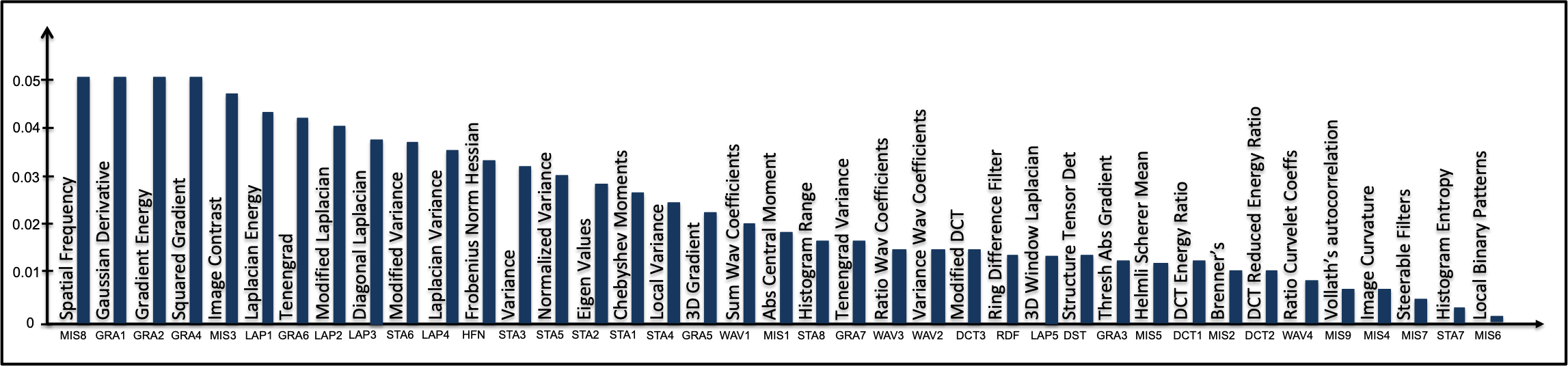
Figure 3: A ranked list of all focus measures used in our analysis. The list is sorted in descending order of the normalized cumulative consensus score $\hat{C}$ computed over our focal stack dataset.

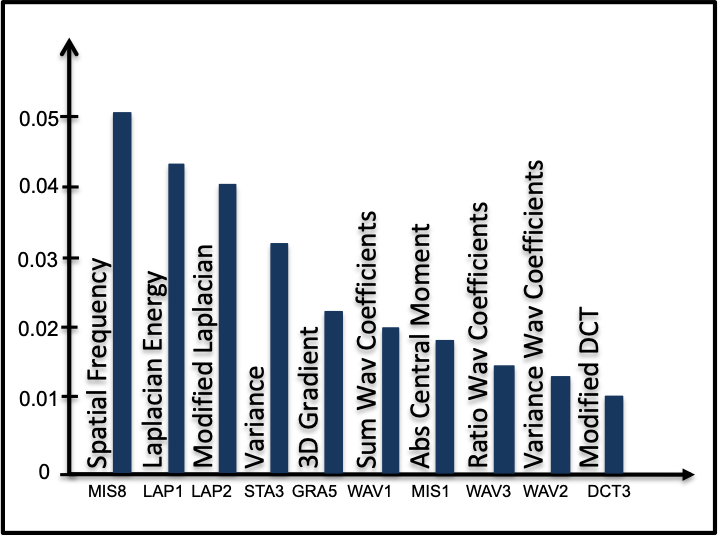
Figure 4: Top 10 focus measures with a high degree of consensus but not high correlation. The normalized consensus score is shown on the Y-axis. This score is used as the weight for creating the composite focus measure.

IV-B Correlation of Focus Measures

The focus measures used in our analysis contain near-identical or highly correlated measures. These will naturally be in consensus with each other but add little additional value. Only one of each highly correlated set of measures is a useful choice for the composite focus measure. We compute pairwise correlation between focus measures across pixels of all focal stacks. This is a cumulative correlation score and is computed as:

$$\hat{C}_{r}(F_{i},F_{j})=\sum_{FS}\sum_{p}\sum_{l}\sqrt{(F_{i}(p,l)-F_{j}(p,l))^{2}},$$ (5)

where FS indicates all focal stacks, p indicates all the pixels in a focal slice and $l$ indicates the slices in the stack.

Figure 5 shows the pairwise correlation between all pairs of measures across the focal stack dataset. From left-to-right and top-to-bottom, the measures are arranged in descending order of consensus $\hat{C}$. We seek to cluster these measures and only select one representative from each cluster. The similarity between focus measures encoded in the correlation matrix of Figure 5 can be used to cluster them. We apply hierarchical agglomerative clustering on the distance matrix (reciprocal of the similarity matrix) to cluster correlated focus measures.

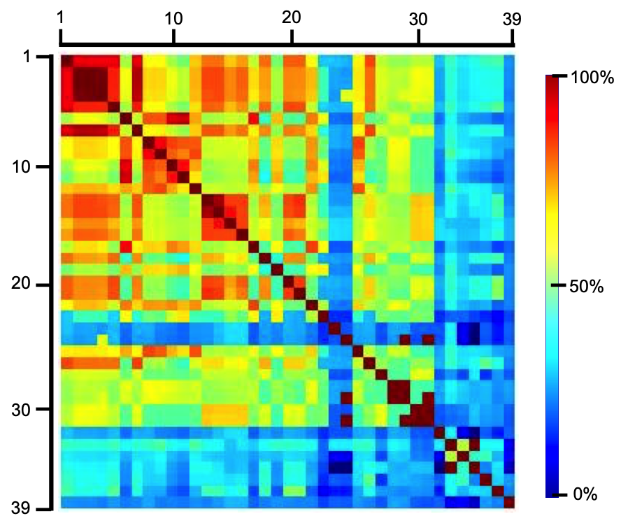
Figure 5: Percentage pairwise correlation between pairs of focus measures (best viewed in color). The FMs from left-to-right and top-to-bottom follow the same ordering shown in the ranked consensus list of Fig. 3. FMs in dark shades of red indicate high correlation. It is evident that the first five measures in descending order of consensus are all highly correlated with each other. We would like to retain only one measure from these.

We invert the correlation score between all pairs of measures to compute a distance $d_{F_{i},F_{j}}=\hat{C}_{r}(F_{i},F_{j})^{-1}$. Agglomerative clustering is then applied with the single-linkage criterion, which specifies the distance $D$ between clusters $c_{i}$ and $c_{j}$ as the minimum distance between all the measures belonging to the clusters:

$$D(c_{i},c_{j})=\underset{F_{i}\in c_{i},F_{j}\in c_{j}}{min}\,d_{F_{i},F_{j}}$$ (6)

The optimal number of clusters is computed using the gap statistic [43] that uses the cumulative within-cluster distance $W_{m}$ for all candidate number of clusters m as

$$W_{m}=\sum^{m}_{n=1}\sum_{F_{i},F_{j}\in c_{n}}d_{F_{i},F_{j}},$$ (7)

which is the sum of distances between measures belonging to the same cluster. The optimal cluster count is set to the point at which the logarithmic plot of the within-cluster distance $W_{m}$ exhibits an elbow or begins to flatten out.

We arrive at an optimal number of $23$ clusters for the $N_{F}=39$ measures used in our analysis. The dendrogram for this clustering is shown in Figure 6. We use the measure with the highest $\hat{C}$ as the representative measure for each cluster. We further sort all the representative measures based on $\hat{C}$. The top ten focus measures that exhibit high consensus but not high correlation are shown in the list in Figure. 4.

A weighted combination of the top five focus measures of Figure 4 forms our composite focus measure (cFM). The weight for each measure is its normalized cumulative consensus score. More measures from this list can be used for focus measurement at the cost of more computation but the benefit of adding measures keeps decreasing as the list is traversed, as elaborated in [30].

IV-C Evaluation of the cFM

To verify whether the computed cFM is universal, we re-compute the consensus for all focus measures using Equation 2, but the data term for each pixel is computed using only the ten measures from the composite measure of Figure 4. The correlation scores between the measures remain unchanged. We observe that there is no re-ordering in the composite measure on re-computing consensus scores, confirming the robustness of the computed composite measure.

To confirm the generalization of the cFM, we evaluate the consensus and correlation of focus measures for different subsets of our focal stack dataset. We isolate four subsets containing 50 focal stacks each. The subsets are selected based on scene attributes such as texture complexity, amount of blur, type of illumination and random selection. Table I shows the top-five composite measure for the four subsets of (1) scenes with high texture, (2) scenes with high degree of blur, (3) outdoor scenes with bright illumination, (4) random subset of 50 focal stacks. Such a categorization has little impact on the composite measure, the only difference being that the HFN measure does not cluster within the LAP2 family for densely textured scenes. Overall, the top five measures are consistent and similar, suggesting that the composite measure is general.

0	Full Dataset	MIS8	LAP1	LAP2	STA3	GRA5
1	Dense Textures	MIS8	LAP1	LAP2	HFN	STA3
2	High Defocus	MIS8	LAP1	LAP2	STA3	GRA5
3	Outdoor Illumination	MIS8	LAP1	LAP2	STA3	GRA5
4	Random subset (50)	MIS8	LAP1	LAP2	STA3	GRA5

TABLE I: The top-five measures in the cfm show very little change on using different subsets of the focal stack dataset.

We refer the reader to our previous work [30] where the a similar composite focus measure is used for depth-from-focus. While we proposed an empirical method to compute the composite focus measure in [30], in this work, we have described a more structured approach to cluster correlated focus measures across a larger dataset of focal stacks. The overall similarity in the composite measure suggests that is quite general. In this work, we use the composite focus measure to estimate the in-focus pixels within a focal stack.

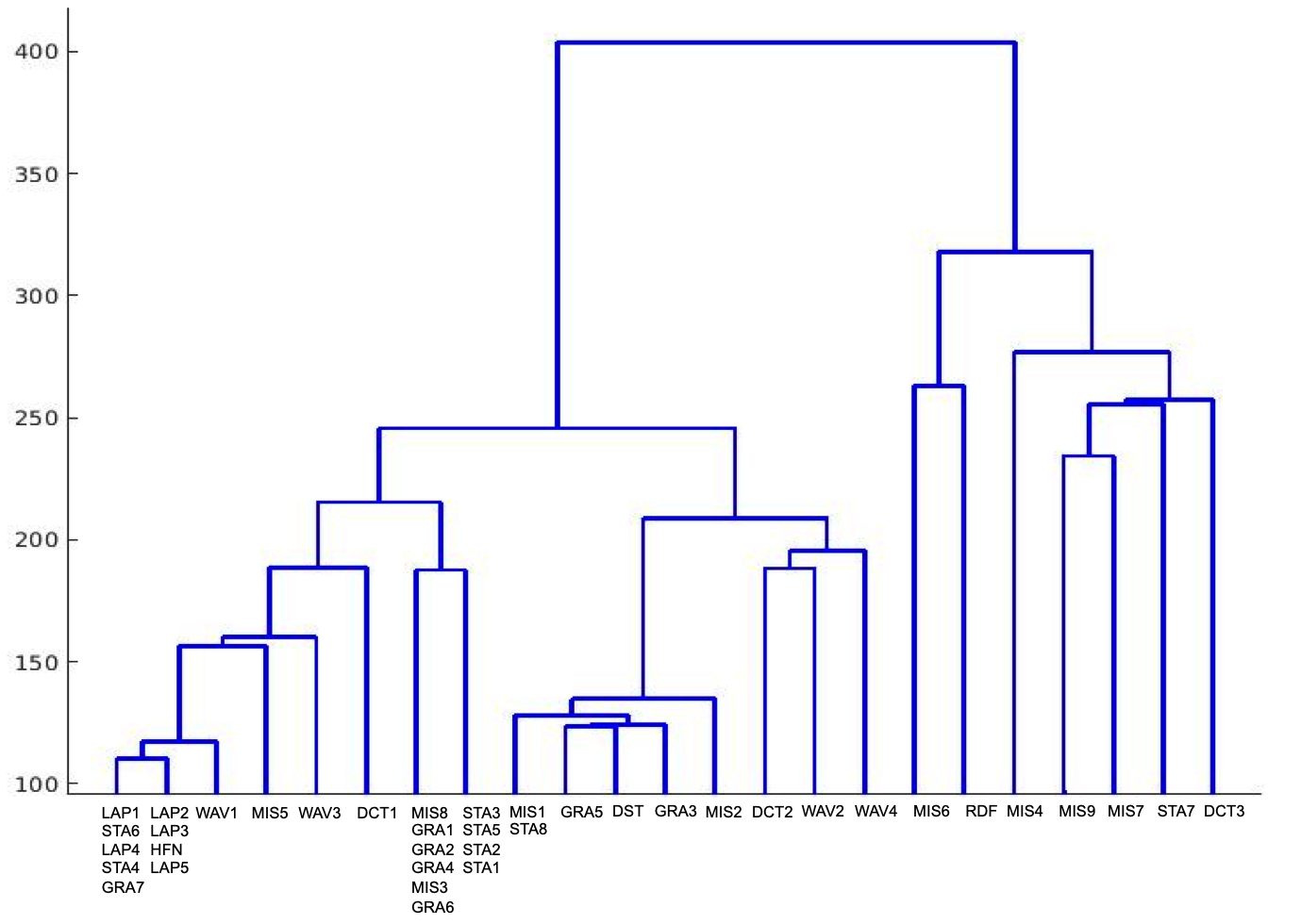
Figure 6: 23 Optimal clusters selected using the GAP statistic [43] applied with hierarchical agglomerative clustering on the correlation matrix of Figure 5.

V Focus Representation

The composite focus measure can be used to build a compact model for focal stacks. We propose a representation for focal stacks that consists of the in-focus intensity for each pixel, a secondary dual focus intensity wherever applicable, bokeh scaling of the intensity value wherever applicable, and the defocus kernel at the pixel at all slices of the captured focal stack. This representation of focus is compact compared to the full focal stack and encodes all high-level and fine characteristics of visible scene points.

V-A In-focus Pixels

The composite focus measure applied at each pixel of a focal stack provides an estimate of the amount of focus of the pixel in each slice. In general, the response of a focus measure across a focal volume is most reliable and informative at high gradients. The reliable in-focus location at high-gradient pixels can be propagated to other pixels based on image content. We follow a similar principle to identify the in-focus position for all pixels.

We use cost-volume filtering [17] to generate a smooth focus map $\cal{I}$ which encodes the slice at which each pixel exhibits a focus peak. A cost volume, representing the cost of labeling a pixel to a focus location, is created with $k$ nodes for each pixel, where $k$ denotes the number of slices in stack. The cost of labeling a pixel $p$ to a location $l$ is computed as:

$$C^{v}_{l}(p)=cFM(p,l)^{-1},$$ (8)

where, $cFM(p,L)$ is the response of the cFM evaluated at pixel $p$ in slice $l$. The cost at each node is inversely proportional to the response of the cFM. Edge-aware filtering [44] of the cost volume based on a guidance image can be used to propagate confident in-focus labels to all pixels. We generate a guidance image by choosing the focal slice for which the cFM is maximized at each pixel. This is a neighborhood-agnostic image and provides a coarse but useful approximation of depth-edges. The final focus map ${\cal I}$ can be computed as the location of minimum cost for each pixel $p$ in the filtered cost volume $C^{v^{\prime}}$.

$${\cal I}(p)=\arg\min_{i=1}^{k}C^{v^{\prime}}_{i}(p)$$ (9)

Figure 7 illustrates a few examples of focus maps computed using the composite focus measure and cost volume filtering.

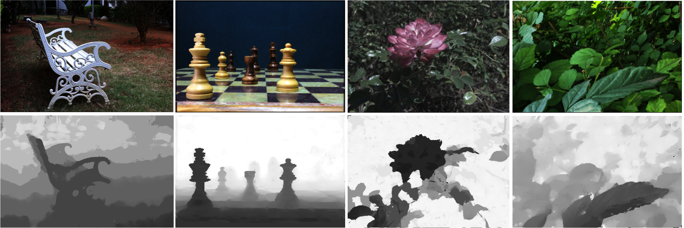
Figure 7: Left-to-right: In-focus image $F_{{\cal I}}$ and focus map ${\cal I}$ for focal stacks captured using Canon EOS 70D, Canon EOS 1100D, Lytro Illum and the Apple iPhone 6.

V-B Dual-focus Pixels

The focus map ${\cal I}$ represents the location of best focus for each pixel. This may not be the only focus distance at which the pixel is in-focus. In some situations, focusing on the background leads to foreground objects being defocused by a large extent such that the background objects become visible through them. The pixels at the edges of the foreground object will now be in-focus at two focal slices, both of which must be considered for accurate geometric modeling of the scene. In principle, it is possible that a single pixel has more than two in-focus slice candidates. However, this situation is impractical given the exponential increase in size of the depth-of-field with increasing depth.

We identify pixels with dual-focus locations using the composite focus measure. This is a crucial attribute of wide-aperture images which is not considered by previous methods dealing with focal stacks. The result of cost volume filtering is a cost vector which can be reciprocated to build a focus vector for each pixel in the scene. The maxima of this vector indicates the location of best focus and is already encoded in ${\cal I}$. We estimate secondary peaks by applying non-maximum suppression to the focus vector for each pixel across focal slices. We seek pixels that show a secondary peak and lie close to a strong gradient to build a dual-focus map ${\cal I}_{d}$.

$${\cal I}_{d}(p)=\left\{\begin{array}[]{cl}l&\textrm{if }cFM(p,l)>cFM(p,l+\Delta l)\\ &\Delta l\in[-w,w]\,\,\&\,\,l\neq{\cal I}(p)\,\,\&\,\,\nabla F_{\cal I}>t_{\nabla}\\ 0&\textrm{otherwise}\end{array}\right\},$$ (10)

where the $w$ parameter encodes a neighborhood of 10$\%$ of focal slices and $t_{\nabla}$ is a threshold on image gradient. The pixels belonging to the dual-focus map ${\cal I}_{d}$ are considered separately for geometric refocusing as described in section VI.

V-C Scaling pixel intensities

Natural scenes may consist of bright scene points corresponding to light-sources or specularities. Camera sensors have a limited dynamic range and very bright scene points usually manifest as uniform saturated intensities. Such pixels do not diminish in intensity even on blurring as their distributed intensity is still higher than the dynamic range of the sensor. This phenomenon is responsible for bokeh circles in wide-aperture images shown in Figure 11.

Pixel that contribute to bokeh circles need to be identified to simulate accurate geometric refocusing of the scene. Drawing inspiration from existing methods such as [22, 29, 34], we identify bokeh-causing pixels as those which have an intensity larger than a threshold $t_{\cal B}$ and do not change their intensity across focal slices:

$${\cal B}(p)=\left\{\begin{array}[]{cl}1&\textrm{if }{\cal G}^{i}(p)>t_{\cal B}\,\,\,\forall i\in[1,k]\\ 0&\textrm{otherwise}\\ \end{array}\right\}.$$ (11)

The focal slice at which the bokeh circle surrounding these points is the smallest is identified as the in-focus slice for the bokeh scene point. All pixels that exhibit bokeh are labeled using a bokeh mask ${\cal B}$. The true intensity of such pixels is identified by scaling up and fitting the appropriate pillbox function that results in the largest bokeh circle around the pixel in the focal stack. These pixels are considered separately for geometric refocusing described in section VI.

The in-focus map ${\cal I}$, the dual-focus map ${\cal I}_{d}$ and the bokeh map ${\cal B}$ form the in-focus representation for scene points. Additionally, we compute $F_{{\cal I}}$ which is a collection of in-focus pixels chosen from their in-focus slice ${\cal I}$. We also compute $F_{{\cal I}_{d}}$ which is a sparse collection of secondary in-focus intensities for pixels that show dual-focus positions. These maps and images efficiently represent the in-focus content of a focal stack.

V-D Defocus Kernels

To estimate the defocus kernels of different pixels, we use the in-focus intensity $F_{{\cal I}}(p)$ of a pixel $p$ as a representation of the luminosity of its scene point. Using this luminosity, we estimate the degree of defocus or the blur-radius for that pixel at other focus positions. Defocused intensities of the points from different depths may contribute to the same pixel on the sensor. We therefore do not use pixels that lie close to depth edges and restrict kernel estimation to equi-focal pixels.

We isolate the pixels that belong to similar regions in depth based on ${\cal I}$. These pixels come from scene points that were close to the same focal plane in the world and are called equi-focal pixels. They appear equally focused (or equally defocused) in any focal slice. The defocus radii of equi-focal pixels can be calibrated in a spatially-invariant manner. The defocus radii of pixels close to a depth-edge can consequently be computed from their nearest equi-focal region.

We use a generative approach to model the defocus kernel that an in-focus pixel subtends at other focal slices. For a defocused scene point, the rays from the point spread out across a defocus kernel of an appropriate size and shape (Figure 1). This can be modeled as an intensity distribution operation from the source pixel to several pixels. Distribution of intensities from a source point is analogous to kernel-splatting methods [45] where each point may have a different contribution. The intensity distributed to a pixel $p$ from its neighbors $q$ can be modeled as:

$$\Delta I_{q}(p)=h(p,q)\circledast F_{{\cal I}}(q)\hskip 12.91663pt\forall q\in N_{p},$$ (12)

where $\Delta I_{q}(p)$ is the intensity that pixel $q$ distributes to pixel $p$, $F_{{\cal I}}(q)$ the intensity of $q$, $N_{p}$ the neighborhood around $p$, $h(x,y)$ the unknown defocus kernel or point-spread-function (PSF) that we would like to model and $\circledast$ denotes convolution. $h$ is typically modeled as a normalized 2D Gaussian kernel with uniform sigma in both axes.

If the above model is restricted to equi-focal pixels, the defocus kernel can be estimated by finding the best spatially invariant convolution kernel that converts a source pixel’s intensity into the target pixel as

$$I(p)=\sum_{q\in N_{p}}\frac{1}{\sigma\sqrt{2\pi}}\mathrm{e}^{(\frac{-d^{2}}{2\sigma^{2}})}F_{{\cal I}}(q),$$ (13)

where, $\sigma$ denotes the space-invariant defocus radius, $d$ the Euclidean distance between pixels $p$ and $q$ and $g(q)$ the focused intensity for each pixel in $N_{p}$. Here $I(p)$ is the rendered intensity of a defocused pixel $p$ and can be compared to different focal slices in ${\cal G}$ to estimate corresponding defocus kernels.

We use geometric calibration to compute the defocus kernels by iterating across equi-focal pixels in a piece-wise manner. We estimate the size and the variable shape of defocus kernels similar to approaches such as [31, 32, 34]. The $\sigma$ of the blur kernel depends on the distance between the current focus position and the pixel’s in-focus position and the shape of the kernel depends on the location of the pixel on the sensor. Pixels towards the edges exhibit vignetting (clipping) and thus result in shortened blur kernels. Figure 8 shows a defocused image of multiple defocused small point light sources captured under low-light conditions. The defocus shapes at the extremeties are visibly shortened compared to those towards the center.

Algorithm 1 Size and Shape of Defocus Kernels

1:procedure $\Pi$($x,y,{\cal I}(x,y),T$)

2:     $s_{xy}\leftarrow|{\cal I}(x,y)-T|$

3:     min $\leftarrow\inf$

4:     $p_{mn}\leftarrow F_{\cal I}(x,y,[m,n])$

5:     $r_{mn}\leftarrow{\cal G}_{T}(x,y,[m,n])$

6:     while $z$ in sizes($s_{xy}$) do

7:         while $h$ in shapes($x,y$) do

8:              $\hat{p}_{mn}\leftarrow gaussianBlur(p_{mn},z,h)$

9:              $d\leftarrow\sum\sum|\hat{p}_{mn}-r_{mn}|$

10:              if $d<min$ then

11:                  $\Pi({\cal I}(x,y),T)\leftarrow(z,h)$

12:                  min $\leftarrow d$                             

13:     return

We estimate blur kernels between all pairs of focal slices using a blur-and-compare framework. For each pair, we use the in-focus pixels $F_{\cal I}$ and compute their largest continuous rectangular region as a reference sub-image. The centre of the rectangular region and its separation from the center of the image is noted to account for vignetting. We then blur the in-focus pixels from one slice with several candidate size and shape parameters and compare the blurred images with the other slice to compute the best match. The shapes are chosen from a set of shapes motivated by [34] and shown in Figure 8. The defocus kernel between a pair of focal slices is computed in a bidirectional manner and the size and shape parameters are recorded for both directions. Algorithm 1 outlines the process of estimating the blur radii between a pair of focal slices.

In Algorithm 1, $p_{mn}$ is a patch of size $[m,n]$ close to pixel $(x,y)$ in $F_{\cal I}$ such that all the pixels in the patch have the same value of ${\cal I}$ and $r_{mn}$ is the corresponding patch from the target focal slice ${\cal G}_{T}$. The collection of tuples $\Pi$ encodes the size and shape of defocus kernels between all pairs of focal slices in a focal stack. Since this is explicitly calibrated for each stack, minor differences in camera design are automatically encoded. $\Pi$ is a collection of at-most $k^{2}$ sizes and $k^{2}$ shapes and thus represents the defocus content within the focal stack in a compact manner.

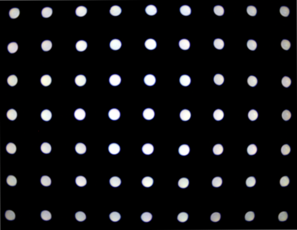
Figure 8: The change in shape of defocus kernels due to vignetting on a Canon 1100D DSLR at f/3.5 with a focal length of 18mm.

We can now represent a focal stack using the ${\cal I},F,{\cal B}$ and $\Pi$ constructs. This is a compact and robust representation that encodes all the focus and defocus properties of the scene points. The ${\cal I}$ maps encode the indices at which the pixel is likely to be in-focus while the $F$ images store photometrically accurate intensities corresponding to these indices, with ${\cal B}$ labeling the pixels that require intensity scaling. The $\Pi$ map encodes the size and shape of defocus that the pixel exhibits in all other not-in-focus slices. The overall storage complexity of our representation is two dense images ${\cal I}$ (single channel) and $F_{\cal I}$ (RGB), three sparse images ${\cal I}_{d}$ (single channel), $F_{{\cal I}_{d}}$ (RGB) and ${\cal B}$ (single channel) and at most $k^{2}$ defocus sizes and shapes. A full focal stack on the other hand stores $k$ RGB images with no implicit information about scene content. Our representation is ideally suited for geometrically accurate and photo-realistic scene refocusing, described in the next section.

VI Geometric Scene Refocusing

We describe a geometric approach to scene refocusing using our representation for focal stacks. Our approach pays explicit attention to fine effects such foreground-background occlusions, mixing of blur kernels at depth-edges, vignetting and bokeh circles. Refocusing is formulated as the task of rendering a target depth-of-field, where the limits of the depth-of-field are defined by focal slice indices $T$ chosen from the unique labels in the focus map ${\cal I}$.

Generating a novel focused image from our representation is a two-step process. The first step is to identify the appropriate intensity for each pixel and the second step is to distribute this intensity to its neighbors based on the defocus kernel at the pixel. We synthesize a refocused image in a piece-wise manner. For all unique labels in the focus map ${\cal I}$, the intensity of the corresponding pixels (or dual-pixels) is considered as the radiance of their scene points. This radiance is scaled appropriately for pixels that also belong to the Bokeh mask ${\cal B}$. The radiance of these pixels is then distributed to its neighbors based on the defocus kernel that pixel subtends on the target focus position. This follows the distributive energy model for wide-aperture images suggested in Equation 12. The pixels in a scene may correspond to different depths and the spatially varying defocus kernels need to be applied in the right order according to the distribution model:

$$\Delta I_{q}(p)=\sum_{q\in N_{p}}H(p,q,\sigma_{q}).F_{\cal I}(q),$$ (14)

where $H(p,q,\sigma_{q})=\frac{1}{\sigma_{q}\sqrt{2R}}\mathrm{e}^{(\frac{-d^{2}}{2\sigma_{q}^{2}})}$ is a Gaussian point spread function with an appropriate $\sigma_{q}$ and corresponding shape.

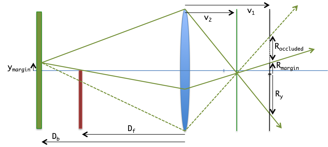
Figure 9: The presence of the foreground partially occludes the background kernel by an amount $R_{occluded}$. The occlusion free component $R_{margin}$ can be computed using $D_{f}$, $D_{b}$, $R_{y}$, $A$ and $y_{margin}$ as shown in Eqn. 16

The order of energy distribution becomes important close to depth-edges. As shown in Figure 9, when the sensor is placed at a position $v_{1}$ which is a near-focus position, the defocused contribution of the background pixels is partially occluded by the presence of the foreground object. Note that our representation consists of dual-focus pixels and captures these pixels behind visible foreground segments. The energy distributed from a background pixel should not freely merge with foreground pixels irrespective of camera and scene geometry. To model the situation shown in Figure 9, we evaluate the impact of partial occlusions in a geometrically accurate manner.

The amount of partial occlusion of the defocus kernel depends on camera and scene geometry while the shape of the occlusion depends on the shape of the depth-edge. The size of the occlusion varies from 0 to 100% from a limiting point above the principal axis to a symmetric point below the principal axis in Figure 9. Figure 10 illustrates three regions of focus that are of importance, one focused beyond the background $a$, the second focused between the foreground and the background $b$ and the third focused closer than the foreground $c$. The occluded portion of defocus kernels is denoted by $o_{a}$, $o_{b}$ and $o_{c}$.

• At a sensor position close to $a$, the foreground pixels are severly defocused and dominate the image content. A small occlusion $o_{a}$ in the defocus kernel of the background has minimal impact on image content.

• At sensor positions close to $b$, the spread of the background pixels overlaps with slightly defocused foreground, however, no background pixel overlaps with in-focus side of foreground pixels (above the principle axis in the diagram). Thus the contribution of a defocused background pixel to a foreground pixel must be disallowed based on the size and shape of $o_{b}$.

• When the sensor plane is focused in front of the foreground such as in position $c$, the background pixel spread overlaps above the principal axis and needs to be shortened based on $o_{c}$.

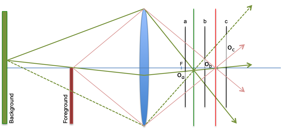
Figure 10: The defocused contribution of background pixels is occluded by the foreground. At sensor positions $a$, $b$ and $c$, the occlusion due to the foreground on the background pixel’s contribution is indicated by the dotted portion $o_{a}$, $o_{b}$ and $o_{c}$ respectively.

To model partial occlusions in our refocusing algorithm, we introduce an occlusion coefficient $\beta$ which geometrically restricts the contribution of a source pixel to a target pixel. The energy distribution model for a pixel is reformulated as

$$\Delta I_{q}(p)=\sum_{q\in N_{p}}\beta_{qp}H(p,q,\sigma_{q}).F_{\cal I}(q).$$ (15)

For background pixels below the occlusion boundary, $F_{{\cal I}_{d}}(q)$ may be used wherever applicable. The occlusion co-efficient is only considered when background-to-foreground mixing occurs, i.e. when ${\cal I}_{q}-{\cal I}_{p}>t_{\beta}$, with $t_{\beta}$ indicating a threshold on number of focal slices. When the precise geometry of the lens and scene is known, the $\beta_{qp}$ parameter can be computed based on the distance between pixels $p$ and $q$ and $R_{margin}$ [28], where,

$$R_{margin}=\frac{R_{q}}{A/2}.\frac{D_{f}}{D_{b}-D_{f}}.y_{margin}.$$ (16)

$D_{f}$ and $D_{b}$ denote the object-side depth for the foreground and background objects, $y_{margin}$ is the distance of source point $y$ from the depth edge on the object side and $R_{q}$ is the geometric kernel radius for pixel $q$ for the current sensor position. The metric units of $R_{margin}$ and $y_{margin}$ can be converted to pixel units. In a focal stack, absolute depth values for source and target pixels $q$ and $p$ may not be known but their relative depth values are indicated by the focus map ${\cal I}$ and the depth ratio can be computed as $\frac{{\cal I}(p)}{{\cal I}(q)-{\cal I}(p)}$. The $y_{margin}$ parameter can be estimated up to an unknown scale factor by calculating the distance of the source pixel from the target pixel in the ${\cal I}$ image. This can be converted to metric units using an approximate estimate of closest and farthest focus positions. Using the Euclidean distance $d$ between pixels $p$ and $q$, the value of $y_{margin}$ can be computed as $y_{margin}=\frac{k{\cal I}(q)+c}{f}\,d,$ where $k$ and $c$ are approximate depths of the nearest and farthest focus positions and $f$ is the focal length of the lens. These constants can be estimated exactly if the capture-time sensor positions are known (using APIs such as MagicLantern). For free-form focal stacks, the constants can be approximated based on the visible scene content. Using these constructs, the occlusion coefficient $\beta_{qp}$ is defined as:

$$\beta_{qp}=\left\{\begin{array}[]{cl}1&\textrm{if }d\leq R_{margin}\\ 0&\textrm{otherwise}\end{array}\right\}.$$ (17)

It may be noted that for dual focus pixels, the sign of $y_{margin}$ is negative and the direction of intensity distribution from the dual pixel is automatically inverted.

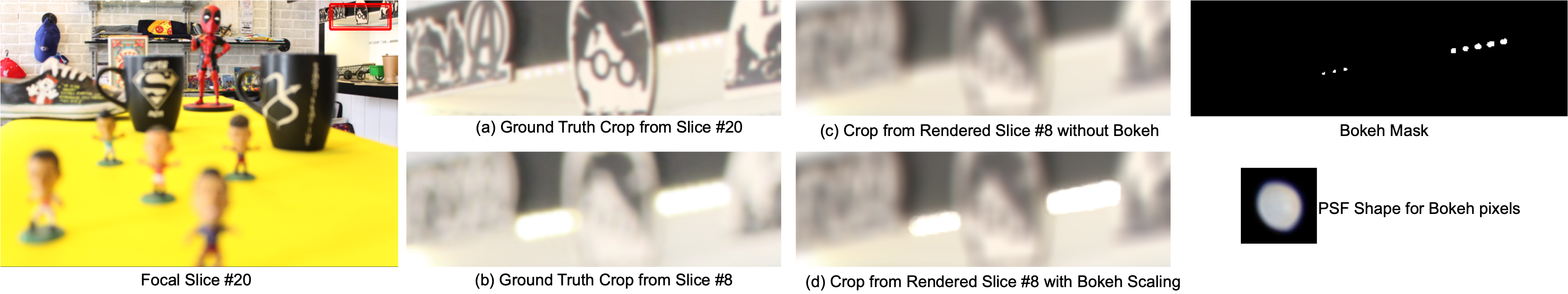
Figure 11: Bokeh simulation using saturated intensities and our geometric refocusing algorithm. The bokeh pixels identified in slice #20 are shown in the Bokeh mask. The asymmetric shape of the point-spread-function is selected from Figure 8 corresponding to the spatial location of the bokeh pixels. The defocused version of figure a using our algorithm without bokeh scaling is shown in figure c (PSNR: 23.5dB, SSIM: 0.90) and with our bokeh scaling approach is shown in figure d (PSNR 28.1dB, SSIM:0.95). Note that our algorithm better simulates intensity saturation visible in the ground-truth figure b.

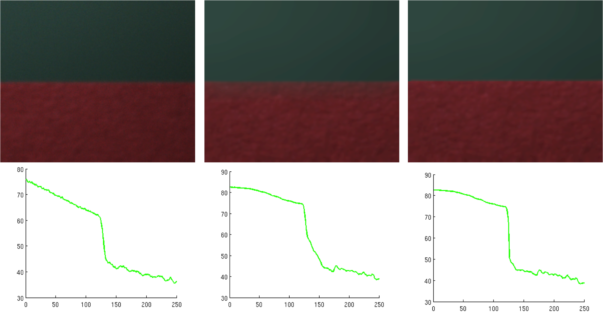
Figure 12: A synthetic red-green depth-edge experiment. The target focus position is similar to $o_{c}$ from Figure 9. From left-to-right: Ground truth image, reconstructed image without $\beta$ and reconstructed image with $\beta$. The second row show the corresponding plots of green intensity from top-to-bottom in the images. Our model with $\beta$ correctly restricts distribution from background to foreground pixels.

Algorithm 2 outlines our overall method for rendering novel focused positions from our representation of a focal stack. In a front-to-back manner, all the focus labels in ${\cal I}$ are considered. A target pixel is generated by accumulating intensities distributed by its neighboring pixels. Bokeh scaling, dual-pixel intensities, partial occlusions at depth-edges and kernel shortening are considered explicitly before intensity distribution.

Algorithm 2 Refocus Scene to Focus Position(s) T

1:procedure refocus(${\cal I},{\cal I}_{d},\Pi,T$)

2:     for all labels $l$ in ${\cal I}$ do

3:         for all pixels $q$ with ${\cal I}(q)=l$ or ${\cal I}_{d}(q)=l$  do

4:              $i_{p}\leftarrow F_{\cal I}(q)$ or $F_{{\cal I}_{d}}(q)$

5:              if ${\cal B}(q)=1$ then

6:                  $i_{q}\leftarrow$ scaleBokeh($i_{q}$)               

7:              for all pixels $p$ neighboring $q$ do

8:                  kernel $\leftarrow\Pi({\cal I}(q),{\cal I}(p))$

9:                  $i_{p}\leftarrow i_{p}+$ applyKernel($i_{q},\beta_{qp},$kernel);

10:                                              

11:     return

VII Experiments & Results

We perform quantitative and qualitative evaluation of our representation in terms of its capability of reconstructing the focal stack and producing novel refocused renderings of the scene. We also compare our method with that of other state-of-the-art methods in post-capture focus control and manipulation.

VII-A Dataset

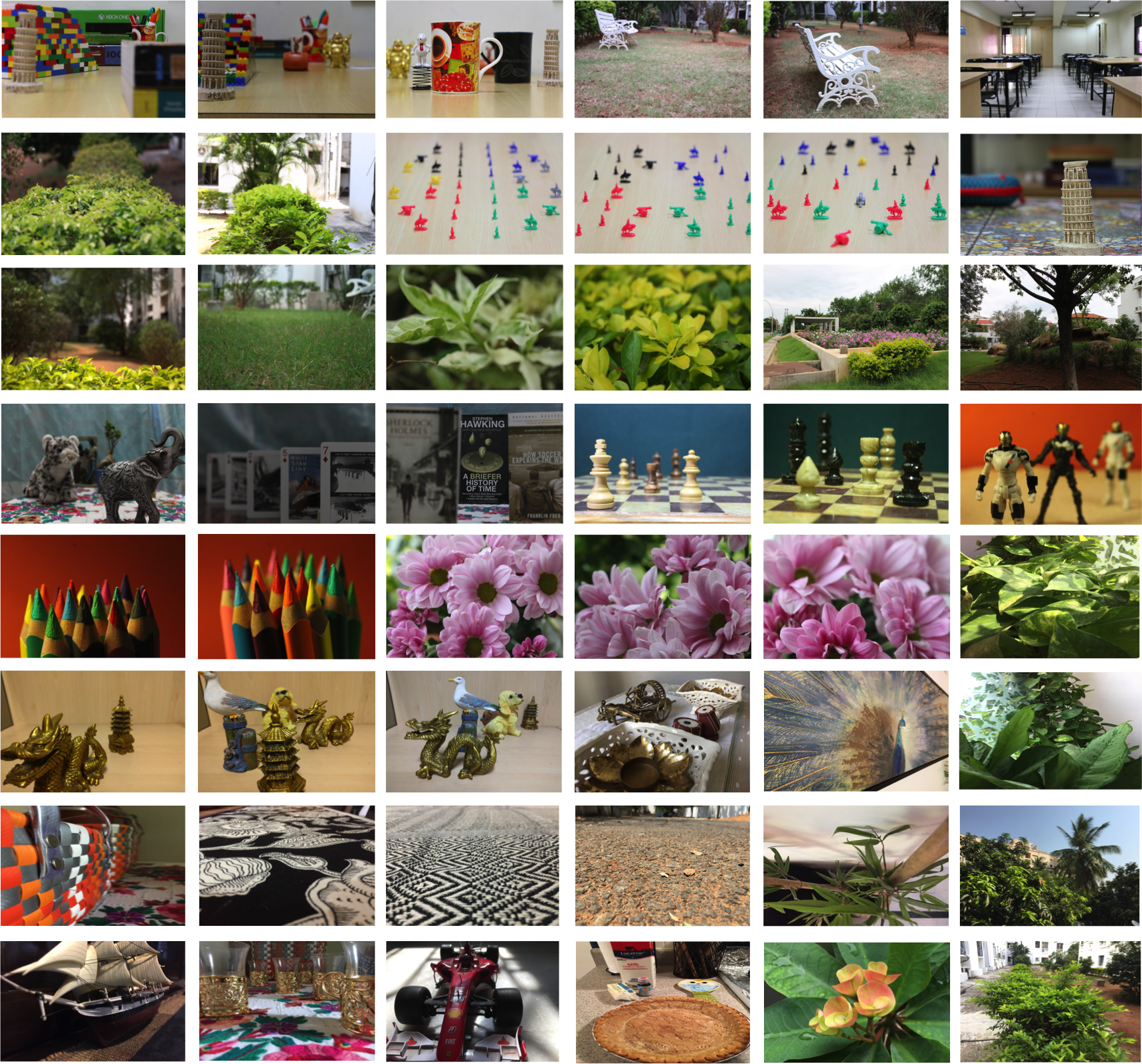
Figure 18: An illustration of the different types of scenes in our focal stack dataset captured using DSLR and mobile cameras.

We use focal stack dataset of about 320 focal stacks. This dataset is composed of 100 focal stacks from the light-field saliency dataset [46], 80 sparsely sampled stationary focal stacks from the Autofocus dataset [47], 20 focal stacks that are available publicly across different works [24] and 120 focal stacks that we captured using DSLR and mobile cameras. Our DSLR focal stacks are captured using Magic Lantern on a Canon EOS 70D and a Canon EOS 1100D. Our mobile focal stacks are captured using an iPhone 6 and an HTC One X (Figure 18). Each focal stack is rescaled to the order of 1M pixels while preserving the aspect ratio. All our experiments are performed on RAW images (or on images rescaled by an appropriate gamma factor). To eliminate pixel misalignment due to magnification, we use the enhanced correlation coefficient maximization approach [48]. The thresholds used in our approach are $t_{\nabla}$=$20$, $t_{\cal B}$=$0.9$ and $t_{\beta}$=$30\%$. To compute the composite focus measure, the response of each focus measure is averaged across three different region of support sizes 3$\times$3, 7$\times$7 and 11$\times$11. The cumulative consensus response for each focus measure is thereby computed across a corpus of about 1.2 billion pixels across the 320 focal stacks.

VII-B Reconstructing Focal Slices

The litmus test for our representation of focus is its ability to reconstruct the focal slices in the stack. The model is expected to not only capture the basic blur profile of scene elements but to also re-create some of the fine transitions at depth-edges. We perform a quantitative and qualitative analysis of the reconstruction quality of our model and refocusing algorithm. Figure 13 illustrates an example on a test focal stack of twenty-slices that is not a part of our focal stack dataset. The figure shows a comparison at three different focus positions - slice 2, slice 9 and slice 18. In the top-row left is the image captured using the camera and in the bottom row is the image refocused using our representation and refocusing algorithm. On a test dataset of ten such focal stacks that were not included in the computation of the composite focus measure, we achieve an average reconstruction PSNR of 41.2 dB per focal slice. This score suggests that our model for focus and refocusing algorithm works well. All images in this paper are best viewed in color.

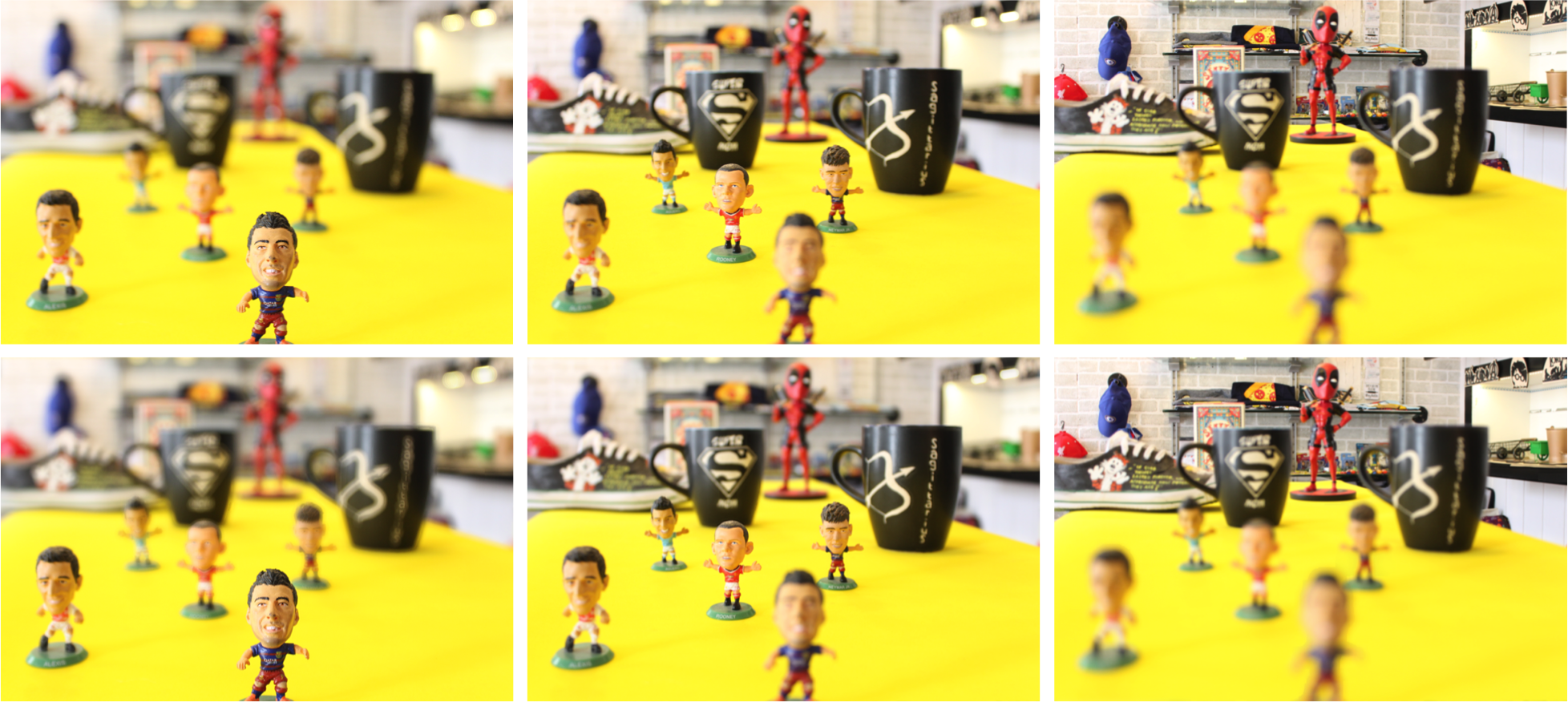
Figure 13: Reconstructed Focal Slices 2, 9 and 18 for a focal stack using our representation and refocusing algorithm. The top-row shows the images captured using a DSLR camera and the bottom row shows the images reconstructed using our representation and our geometric refocusing algorithm.

Ablation Study

To elaborate the impact of the dual-focus representation, the bokeh scaling parameter and the occlusion coefficient, we apply of our refocusing algorithm without the three factors. Figure 14 shows an example where our secondary focus peak estimation is necessary for simulating fine focus effects close to depth edges. Figure 11 demonstrates the benefit of using our bokeh mask for intensity scaling and the application of defocus kernel shortening to simulate vignetting. Figure 15 illustrates the utility of the occlusion co-efficient for accurate focus simulation at deep depth-edges. The qualitative and quantitative improvement provided by our approach is visible across these examples.

To further study the impact of the occlusion co-efficient at depth edges, we capture a focal stack of a test scene consisting of a red foreground plane and a green background plane at fixed distances from the camera. We reconstruct a target focal slice focused in front of the foreground object (similar to $o_{c}$ of Figure 9). We compare this image with a ground-truth focal slice. We quantitatively study the impact of using our defocus model without the occlusion coefficient $\beta$, in which case the green background incorrectly defocuses into the red foreground which is visible on closely observing Fig. 12.

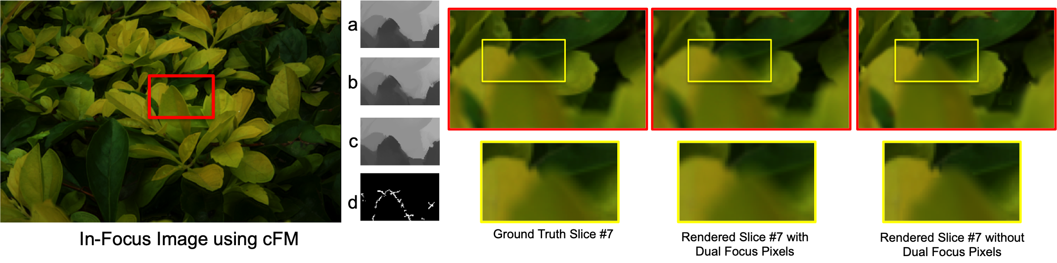
Figure 14: The in-focus image shown on the left is the $F_{\cal I}$ image created using the composite focus measure. Inset (a) shows the focus map ${\cal I}$ on using the LAP2 focus measure alone, inset (b) shows the focus map ${\cal I}$ on using the WAV1 focus measure alone, while inset (c) shows the focus map ${\cal I}$ on using the composite focus measure. Inset (d) is the dual focus pixel map ${\cal I}_{d}$. On using the dual focus pixels, the background dark green leaf is visible through the blurred light green foreground, which is similar to ground truth. Ignoring the dual pixels misses this fine effect as seen in the rightmost image.

Figure 15: First row: Left to right: Simulated focal slice 2 without $\beta$ (PSNR: 34.3dB), true focal slice 2, simulated focal slice 2 using $\beta$ (PSNR 38.8dB). Second row: Insets corresponding to the first row. Notice how the background cuts into the foreground at several leaf edges which is visible in the inset images.

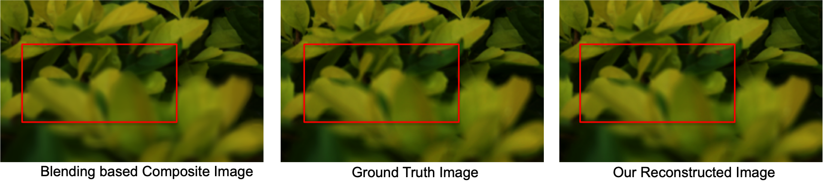
Figure 16: A comparison of blending based focal slice reconstruction of [49] with our geometric algorithm for refocusing. Note the patchy nature of depth-edges in the blending based composite image (PSNR: 28.6dB). The dual focus pixels in our representation enable accurate reconstruction (PSNR: 33.7dB).

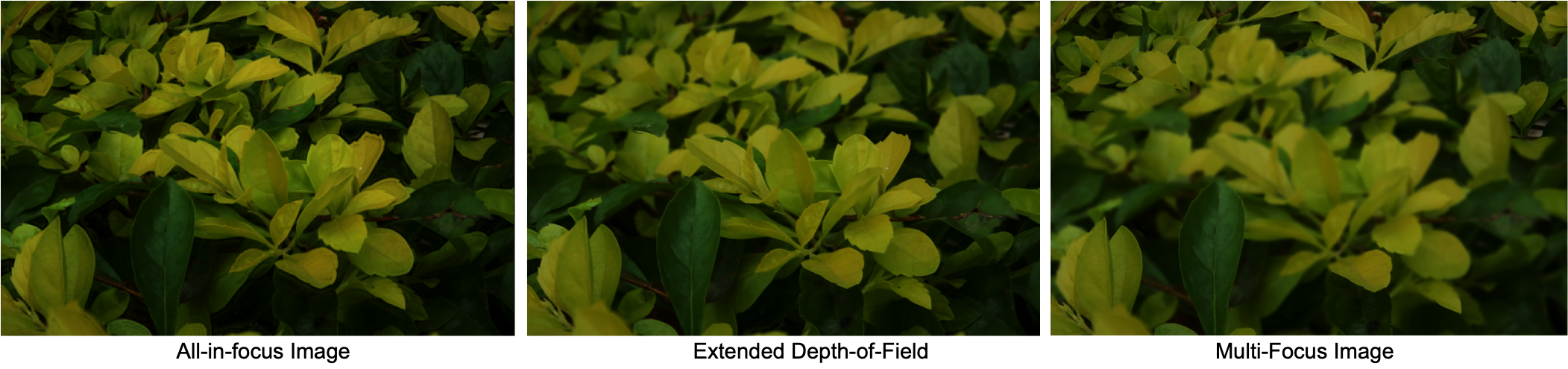
Figure 17: An all-in-focus image (all focal slices in focus), an extended focus image (with multiple contiguous focal slices in focus) and a non-photorealistic image (with non-contiguous focal slices in focus) using our representation and refocusing algorithm.

VII-C Refocusing the Scene

Using our representation, we can create novel focus positions for the scene by changing the target focus position $T$ of algorithm 2. The target position T can be a single focus position chosen from one of the labels in ${\cal I}$ or a set of labels which may or may not be contiguous.

All-in-focus image

In this case, $T$ consists of all labels from ${\cal I}$. The refocusing algorithm collects the in-focus pixels from all labels. Some focal stacks with their focus map and corresponding in-focus image are shown in Figures 7,17.

Extended depth-of-field

When $T$ consists of a contiguous subset of labels from ${\cal I}$, an extended depth-of-field image can be created. The defocus kernels for such an image are chosen from the limiting labels of $T$ on either side. An extended depth-of-field image is shown in Figure 17.

Non-photorealistic Focus

When $T$ consists of multiple disjoint subsets of labels from ${\cal I}$, a non-photorealistic rendering can be created. The defocus kernels can be chosen from the closest limiting label of $T$ for each subset. A non-photorealistic image is shown in Figure 17.

VII-D Comparison

We compare our model with contemporary methods that deal with defocus modeling and post-capture scene refocusing. Previous methods either use specific information such as precise knowledge of focus positions and/or scene depth and mostly do not deal with fine characteristics of wide-aperture images. We provide a quantitative comparison wherever possible. We compare our method with that of [29, 36] for quality of refocusing, [49] for dual-pixel capabilites and [34] for quality of defocus kernels.

Comparison of Refocused Rendering

Jacobs et al. [36] synthesize novel depth-of-field images using focal stacks by defining a target sensor defocus map and generating a rendering closest to that map using ray space analysis. Suwajanakorn et al. [29] also show reconstruction of defocused images from focal stacks however very little details about the process of generation of the defocused images is discussed. A direct comparison with these methods is non-trivial because it requires the ground-truth focus distance for each shot using precisely engineered camera hardware that is not commonly available. Our method compares favourably in the sense that it is independent of the capture-time focus distance as we estimate the focus profile for the scene directly from the focal slices. In addition, we also make use of dual-pixels to accurately reconstruct focus effects at depth-edges as shown in Figure 14. Our method is therefore scalable to generic focal stacks from any camera.

Comparison with Alpha-Blending

Alpha-blending of different focal slices can be applied to generate refocused renderings, as described in Barron et al. [49]. Such methods usually assume an extended canvas of background pixels which are blurred and blended to create a refocused composite. Our dual-focus pixel method identifies the pixel intensity better and thus the textural information at partially occluded background pixel is encoded in our representation. Such awareness of true pixel intensity and color is lost in the mutually exclusive focus textures that are used in blending based methods. In Figure 16, we demonstrate the quantitative benefit of our method over the background-stretched method of [49]. Background textural details becoming apparent through a blurred foreground is clearly visible using our approach.

Comparison of Bokeh Quality

Hach et al. [34] render bokeh highlights using precise modeling and reconstruction of the PSF for a high-quality camera. They tediously calibrate an RGBD camera and learn the distribution of PSFs in order to simulate DoF effects in a post-capture manner. They also describe a kernel stitching algorithm to handle partial occlusions. While their model is designed for a high-end camera with a high dynamic range, we have shown a model which is applicable in a general setting, which works in the presence or absence of depth information. We compute the size and shape of defocus kernels relative to the pixel location in the image and we also apply an intensity scaling to bokeh pixels (Sections V,VI). This leads to natural bokeh effects in our refocused renderings. While the defocus kernels we estimate may not be perfectly shaped for an arbitrary camera, the shortening of kernels due to vignetting and the intensity scaling method creates photo-realistic bokeh, shown qualitatively in Figure 11.

VIII Acknowledgement

This work is under consideration at the Elsevier Computer Vision and Image Understanding Journal.

IX Conclusions

In this paper, we propose a robust model to estimate the focus and defocus properties of a scene from a set of multi-focus images. We propose a composite measure of focus that reliably locates in-focus pixels. We also present a geometric algorithm for refocusing from first principles, preserving the fine effects of focus in challenging geometric situations. Our algorithm renders by distributing each pixel‘s intensity to its neighbors using geometrical kernel sizes and shapes. Pixels close to depth-edges and those with saturated intensities are also accounted for. We show the qualitative and quantitative impact of our representation and refocusing algorithm. Our approach is ideally suited for image editing toolkits requiring precise manipulation of multi-focus imagery.

References

- [1] Hasinoff, S.W., Kutulakos, K.N., Durand, F., Freeman, W.T.: Time-constrained photography. In: IEEE 12th International Conference on Computer Vision, IEEE (2009) 333–340
- [2] Hasinoff, S.W., Kutulakos, K.N.: Light-efficient photography. IEEE Transactions on Pattern Analysis and Machine Intelligence 33(11) (2011) 2203–2214
- [3] Kutulakos, K.N., Hasinoff, S.W.: Focal stack photography: High-performance photography with a conventional camera. In: In IAPR Machine Vision Applications. (2009)
- [4] Sakurikar, P., Narayanan, P.J.: Focal stack representation and focus manipulation. In: 4th IAPR Asian Conference on Pattern Recognition (ACPR). (2017) 250–255
- [5] Kubota, A., Aizawa, K., Chen, T.: Reconstructing dense light field from array of multifocus images for novel view synthesis. IEEE Transactions on Image Processing 16(1) (2007) 269–279
- [6] Kodama, K., Kubota, A.: Efficient reconstruction of all-in-focus images through shifted pinholes from multi-focus images for dense light field synthesis and rendering. IEEE Transactions on Image Processing, 2013 (2013)
- [7] Sakurikar, P., Narayanan, P.: Dense view interpolation on mobile devices using focal stacks. In: IEEE Conference on Computer Vision and Pattern Recognition Workshops (CVPRW), 2014, IEEE (2014) 138–143
- [8] Nagahara, H., Kuthirummal, S., Zhou, C., Nayar, S.K.: Flexible depth of field photography. In: European Conference on Computer Vision – ECCV 2008. Springer (2008) 60–73
- [9] Kuthirummal, S., Nagahara, H., Zhou, C., Nayar, S.: Flexible depth of field photography. IEEE Transactions on Pattern Analysis and Machine Intelligence 33(1) (2011) 58–71
- [10] Agarwala, A., Dontcheva, M., Agrawala, M., Drucker, S., Colburn, A., Curless, B., Salesin, D., Cohen, M.: Interactive digital photomontage. In: ACM Transactions on Graphics (TOG). Volume 23., ACM (2004)
- [11] Nayar, S.K., Nakagawa, Y.: Shape from focus. IEEE Transactions on Pattern Analysis and Machine Intelligence 16(8) (1994) 824–831
- [12] Helmli, F.S., Scherer, S.: Adaptive shape from focus with an error estimation in light microscopy. In: ISPA 2001. Proceedings of the 2nd International Symposium on Image and Signal Processing and Analysis. (2001) 188–193
- [13] Murali Subbarao, Tae-Sun Choi, A.N.: Focusing techniques. Optical Engineering 32 (1993) 32 – 32 – 13
- [14] Shen, C.H., Chen, H.H.: Robust focus measure for low-contrast images. In: 2006 Digest of Technical Papers International Conference on Consumer Electronics. (2006) 69–70
- [15] Yang, G., Nelson, B.J.: Wavelet-based autofocusing and unsupervised segmentation of microscopic images. In: Proceedings 2003 IEEE/RSJ International Conference on Intelligent Robots and Systems (IROS 2003) (Cat. No.03CH37453). Volume 3. (2003)
- [16] Zhou, C., Miau, D., Nayar, S.K.: Focal sweep camera for space-time refocusing. Technical Report, Department of Computer Science, Columbia University CUCS-021-12 (2012)
- [17] Rhemann, C., Hosni, A., Bleyer, M., Rother, C., Gelautz, M.: Fast cost-volume filtering for visual correspondence and beyond. In: 2011 IEEE Conference on Computer Vision and Pattern Recognition (CVPR), IEEE
- [18] Boykov, Y., Veksler, O., Zabih, R.: Fast approximate energy minimization via graph cuts. IEEE Transactions on Pattern Analysis and Machine Intelligence 23 (2001) 2001
- [19] Kubota, A., Takahashi, K., Aizawa, K., Chen, T.: All-focused light field rendering. In: Proceedings of the Fifteenth Eurographics conference on Rendering Techniques. EGSR’04 (2004) 235–242
- [20] Pertuz, S., Puig, D., Garcia, M.A.: Analysis of focus measure operators for shape-from-focus. Pattern Recognition 46(5) (2013) 1415 – 1432
- [21] Möller, M., Benning, M., Schönlieb, C.B., Cremers, D.: Variational depth from focus reconstruction. IEEE Trans. Image Processing 24 (2015) 5369–5378
- [22] Surh, J., Jeon, H.G., Park, Y., Im, S., Ha, H., Kweon, I.S.: Noise robust depth from focus using a ring difference filter. In: IEEE Conference on Computer Vision and Pattern Recognition. (2017)
- [23] Mahmood, M.T., Majid, A., Choi, T.S.: Optimal depth estimation by combining focus measures using genetic programming. Information Sciences 181(7) (April 2011) 1249–1263
- [24] Boshtayeva, M., Hafner, D., Weickert, J.: A focus fusion framework with anisotropic depth map smoothing. Pattern Recognition 48(11) (2015) 3310 – 3323
- [25] Chaudhuri, S., Rajagopalan, A.N.: Depth from defocus: a real aperture imaging approach. Springer Science & Business Media (2012)
- [26] Favaro, P., Soatto, S.: A geometric approach to shape from defocus. IEEE Transactions on Pattern Analysis and Machine Intelligence 27(3) (2005) 406–417
- [27] Persch, N., Schroers, C., Setzer, S., Weickert, J.: Introducing More Physics into Variational Depth–from–Defocus. In: Pattern Recognition: 36th German Conference, GCPR. Springer (2014) 15–27
- [28] Bhasin, S.S., Chaudhuri, S.: Depth from defocus in presence of partial self occlusion. In: Proceedings. Eighth IEEE International Conference on Computer Vision, 2001. Volume 1. (2001) 488–493 vol.1
- [29] Suwajanakorn, S., Hernandez, C., Seitz, S.M.: Depth from focus with your mobile phone. In: The IEEE Conference on Computer Vision and Pattern Recognition (CVPR). (June 2015)
- [30] Sakurikar, P., Narayanan, P.J.: Composite focus measure for high quality depth maps. In: 2017 IEEE International Conference on Computer Vision (ICCV). (2017) 1623–1631
- [31] Kee, E., Paris, S., Chen, S., Wang, J.: Modeling and removing spatially-varying optical blur. In: 2011 IEEE International Conference on Computational Photography (ICCP). (2011) 1–8
- [32] Shih, Y., Guenter, B., Joshi, N.: Image enhancement using calibrated lens simulations. In Fitzgibbon, A., Lazebnik, S., Perona, P., Sato, Y., Schmid, C., eds.: European Conference on Computer Vision, Springer (2012) 42–56
- [33] Tang, H., Kutulakos, K.N.: What does an aberrated photo tell us about the lens and the scene? In: IEEE International Conference on Computational Photography (ICCP). (2013) 1–10
- [34] Hach, T., Steurer, J., Amruth, A., Pappenheim, A.: Cinematic bokeh rendering for real scenes. In: Proceedings of the 12th European Conference on Visual Media Production. CVMP ’15 (2015) 1:1–1:10
- [35] Matsui, S., Nagahara, H., Taniguchi, R.I.: Half-sweep imaging for depth from defocus. In: Advances in Image and Video Technology. Springer (2012) 335–347
- [36] Jacobs, D.E., Baek, J., Levoy, M.: Focal stack compositing for depth of field control. Stanford Computer Graphics Laboratory Technical Report 1 (2012)
- [37] Ng, R., Levoy, M., Brédif, M., Duval, G., Horowitz, M., Hanrahan, P.: Light field photography with a hand-held plenoptic camera. Computer Science Technical Report CSTR 2(11) (2005)
- [38] : Lytro. https://www.lytro.com/
- [39] Sakurikar, P., Mehta, I., Balasubramanian, V.N., Narayanan, P.J.: Refocusgan: Scene refocusing using a single image. In: The European Conference on Computer Vision (ECCV). (September 2018)
- [40] Sakurikar, P., Mehta, I., Narayanan, P.J.: Defocus magnification using conditional adversarial networks. In: Winter Conference on Applications of Computer Vision (WACV). (January 2019)
- [41] Lijun, W., Xiaohui, S., Jianming, Z., Oliver, W., Chih-Yao, H., Sarah, K., Huchuan, L.: Deeplens: Shallow depth of field from a single image. ACM Trans. Graph. (Proc. SIGGRAPH Asia) 37(6) (2018) 6:1–6:11
- [42] Brown, M.: From raw to srgb and back: Modeling the onboard camera processing. https://www2.securecms.com/ICIP2013/Tutorial_T3.asp
- [43] Tibshirani, R., Walther, G., Hastie, T.: Estimating the number of clusters in a data set via the gap statistic. Journal of the Royal Statistical Society: Series B (Statistical Methodology) 63(2) (2001) 411–423
- [44] He, K., Sun, J., Tang, X.: Guided image filtering. IEEE Transactions on Pattern Analysis and Machine Intelligence, (2013)
- [45] Gharbi, M., Li, T.M., Aittala, M., Lehtinen, J., Durand, F.: Sample-based monte carlo denoising using a kernel-splatting network. ACM Trans. Graph. 38(4) (2019) 125:1–125:12
- [46] Zhang, J., Wang, M., Lin, L., Yang, X., Gao, J., Rui, Y.: Saliency detection on light field: A multi-cue approach. ACM Trans. Multimedia Comput. Commun. Appl. 13(3) (July 2017) 32:1–32:22
- [47] Abuolaim, A., Punnappurath, A., Brown, M.S.: Revisiting autofocus for smartphone cameras. In: The European Conference on Computer Vision (ECCV). (September 2018)
- [48] Evangelidis, G., Psarakis, E.: Parametric image alignment using enhanced correlation coefficient maximization. IEEE Transactions on Pattern Analysis and Machine Intelligence 30(10) (2008) 1858–1865
- [49] Barron, J.T., Adams, A., Shih, Y., Hernández, C.: Fast bilateral-space stereo for synthetic defocus. In: 2015 IEEE Conference on Computer Vision and Pattern Recognition (CVPR). (2015) 4466–4474