3D MHD Simulations of Accretion onto Stars with Tilted Magnetic and Rotational Axes

Abstract

We present results of global three-dimensional (3D) magnetohydrodynamic (MHD) simulations of accretion onto magnetized stars where both the magnetic and rotational axes of the star are tilted about the rotational axis of the disc. We observed that initially the inner parts of the disc are warped, tilted, and precess due to the magnetic interaction between the magnetosphere and the disc. Later, larger tilted discs form with the size increasing with the magnetic moment of the star. The normal vector to the discs are tilted at different angles, from $\sim 5^{\circ}-10^{\circ}$ up to $\sim 30^{\circ}-40^{\circ}$. Small tilts may result from the winding of the magnetic field lines about the rotational axis of the star and the action of the magnetic force which tends to align the disc. Another possible explanation is the magnetic Bardeen-Petterson effect in which the disc settles in the equatorial plane of the star due to precessional and viscous torques in the disc. Tilted discs slowly precess with the time scale of the order of $\sim 50$ Keplerian periods at the reference radius ($\sim 3$ stellar radii). Our results can be applied to different types of stars where evidence of tilted discs and/or slow precession has been observed.

1 Introduction

Different types of disc-accreting stars have strong magnetic fields, such as young T Tauri stars (e.g., Bouvier et al. 2007), accreting X-ray pulsars (e.g., van der Klis 2006), and white dwarfs (intermediate polars, e.g., Warner et al. 1995, 2004; Hellier 2001). The magnetospheres of these stars open magnetospheric gaps in the surrounding accretion discs, giving rise to complex paths of accretion onto the star. Many observational properties of these stars are determined by the disc-magnetosphere interactions.

The magnetic field of stars may be complex (e.g., Johns-Krull 2007). However, at large distances, the dipole component often dominates and is responsible for the disc-magnetosphere interaction (e.g., Long et al. 2007, 2008; Gregory 2011). Spectropolarimetric observations show that in many young stars, the dipole component of the field is tilted about the rotational axis of the star by an angle, $\theta\sim 10^{\circ}-20^{\circ}$ (e.g., Donati et al. 2007, 2010, 2011). In general, the rotational axis of the star can also be tilted with respect to the rotational axis of the disc. Such misalignments may result from the varying angular momentum directions of the gas that falls onto the disc, as expected in the assembly of protoplanetary discs.

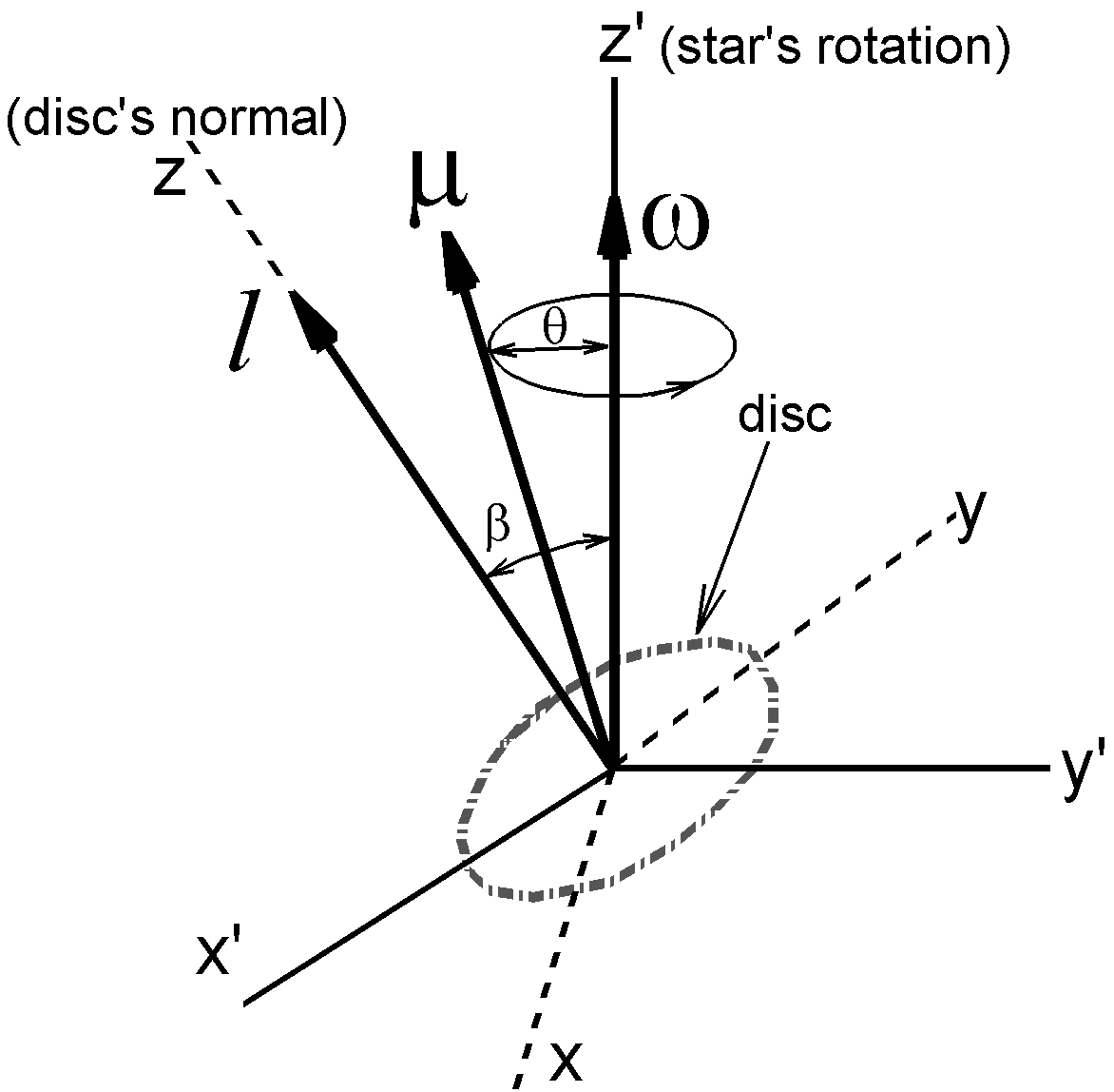
Figure 1: Sketch shows coordinate systems used in the paper. The coordinate system $x^{\prime}y^{\prime}z^{\prime}$ is used in numerical simulations. In this system, the $z^{\prime}-$axis is along the direction of the star’s angular velocity vector, $\omega$. The stellar dipole moment, $\mu$ is tilted about $\omega$ by angle $\theta$. The local disc’s angular momentum vector, $l$ is directed along the $z-$axis and is tilted by an angle $\beta$ with respect of $\omega$. Initially, at $t=0$, the disc is located at the $xy-$plane. The coordinate system $xyz$ is used in our 3D plots.

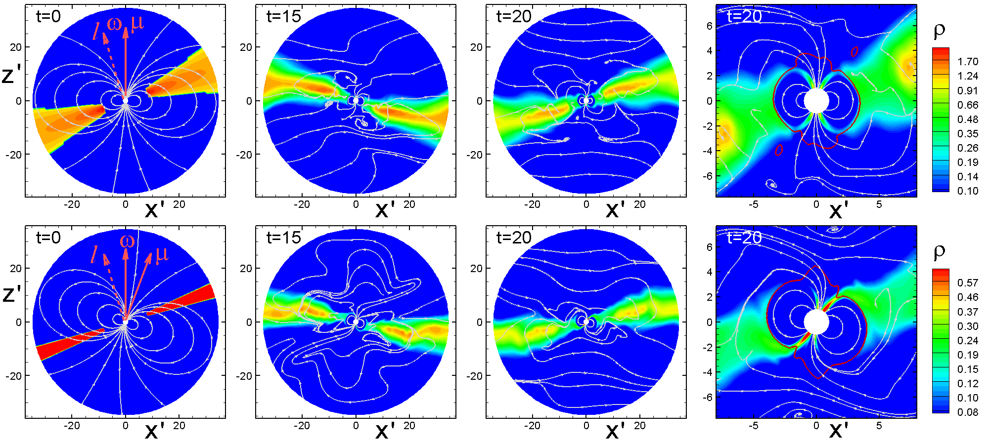
Figure 2: $x^{\prime}z^{\prime}-$slices of density distribution in models A and B (top and bottom panels, respectively) at $t=0$, $t=15$, and $t=20$. Top and bottom right panels show close view of matter flow near the magnetosphere at $t=20$. White lines show sample poloidal magnetic field lines. Red lines show the $\beta_{1}=1$ line. In this and other 2D plots we use the coordinate system $x^{\prime}y^{\prime}z^{\prime}$ (see Fig. 1).

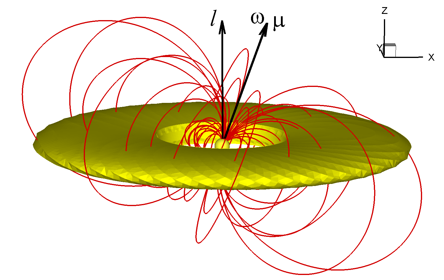
Figure 3: 3D view of the disc at $t=0$ in Model A. The color background shows one of the density levels ($\rho=1.7$ in dimensionless units). Lines are selected field lines. Arrows show directions of the disc’s angular momentum vector, $l$, the star’s angular velocity vector, $\omega$, and the stellar dipole moment, $\mu$. In this and other 3D plots we use the coordinate system $xyz$, where the $z-$axis is along the initial direction of $l$ (see Fig. 1).

Interaction of the inner disc with the tilted magnetosphere leads to bending torques in the disc, which result in a warp (bending wave) in the inner disc (e.g., Bouvier et al. 1999; Terquem & Papaloizou 2000; Romanova et al. 2013). If the rotation axis of the star is aligned with that of the disc, the warp rotates with the period of the star, and on average, the bending torque on the inner disc is zero (e.g., Lai 1999). However, if the rotational axis of the star is tilted about the rotational axis of the disc, then the time-averaged torque on the inner disc is not zero, and the inner parts of the disc may be warped systematically (e.g., Aly 1980; Lipunov & Shakura 1980; Lai 1999). The magnetic torque also may drive the tilted inner disc into retrograde precession (opposite to the rotation of the disc) around the rotational axis of the star. Under some conditions the combined effects of differential precession and viscosity tend to drive the inner disc toward an aligned state, where the disc plane lies in the rotational equator of the star (the magnetic Bardeen-Petterson effect, Lai 1999). Thus, the magnetic warping torque and the magnetic Bardeen-Petterson effect have an opposite consequence in the inner disc orientation; which effect wins depends on the dissipative properties of the inner disc and other parameters (such as the tilt of the magnetosphere).

In theoretical studies, the configuration of the magnetosphere interacting with the disc was presented in the analytical form and was not fully time-dependent (e.g., Aly 1980; Lipunov & Shakura 1980; Lai 1999). Here, we show results of the global 3D MHD time-dependent numerical simulations of this problem, where the configuration of the magnetic field varies in time and depends on the relative motion of the rotating star and the disc.

Earlier, we performed global 3D MHD simulations of accretion onto a star with a tilted dipole magnetosphere, where the rotational axis of the star was aligned with the rotational axis of the disc (Romanova et al. 2003, 2004, 2013; Romanova & Owocki 2015; see also Zhilkin & Bisikalo 2010). In our new simulations, we study numerically accretion onto stars where both the rotational and magnetic axes are tilted.

We performed simulations at a variety of different parameters and observed that a significant part of the disc becomes tilted. However, in some models the disc normal tends to be aligned with the rotational axis of the star (aligned discs), while in other models it is systematically tilted. Comparisons of models show that an important parameter determining the final tilt is the position of the inner disc relative to the dipole magnetosphere. Higher tilts were observed in models where the disc is closer to the star and stronger magnetic field threads the disc. Another parameter is the rotation of the star: higher tilts are observed in stars with faster rotation.

In Sec. 2 we review the theory. In Sec. 3 we describe our numerical model. In Sec. 4, 5 and 6 we show results of simulations. Discussion and conclusions are given in Sec. 7.

2 Overview of the theory

Below, we briefly review the theory following the approach of Lai (1999) and Foucart & Lai (2011) (see also Aly 1980; Lipunov & Shakura 1980; Lai et al. 2011).

2.1 Warping instability

We consider a star of mass $M_{\star}$ and radius $R_{\star}$ which rotates with an angular velocity ${\mbox{\boldmath$\omega$}}=\omega\hat{{\mbox{\boldmath$\omega$}}}$, where $\hat{{\mbox{\boldmath$\omega$}}}$ is the unit vector. The rotational axis of the star $\hat{{\mbox{\boldmath$\omega$}}}$ is tilted about the disc’s angular momentum vector $l$ by an angle $\beta$. We suggest that a star has a dipole magnetic field and place the magnetic moment $\mu$ at an angle $\theta$ relative to $\omega$. Vector $\mu$ rotates about $\omega$ with angular velocity of the star, $\omega$ (see sketch in Fig. 1).

Matter of the disc accreting with the rate $\dot{M}$ is stopped by the magnetosphere of the star at the magnetospheric radius (e.g., Pringle and Rees 1972; Ghosh & Lamb 1978):

$$r_{m}=k\left({\mu^{4}\over GM_{\star}\dot{M}^{2}}\right)^{1/7},$$ (1)

where $k\approx 0.5$ (e.g., Long et al. 2005; Bessolaz et al. 2008).

The tilted magnetosphere interacts with the inner parts of the accretion disc. Such interaction may lead to warping and precession of the disc. For analysis of the disc warping, we use the coordinate system $xyz$, with the $z-$axis initially directed along the disc normal $\hat{\mbox{\boldmath$l$}}$. We use the variable $\hat{\mbox{\boldmath$l$}}$ to indicate the initial position of the disc normal. We suggest that the direction of the disc normal may change in time and we use the variable $\hat{\mbox{\boldmath$l$}}_{n}$ for the disc normal of warping disc. We also use the variable $\beta_{n}$ for changing angle between the disc normal $\hat{\mbox{\boldmath$l$}}_{n}$ and $\hat{{\mbox{\boldmath$\omega$}}}$.

The vertical (perpendicular to the disc) magnetic field produced by the stellar dipole is given by

$$B_{z}=-{\mu\over r^{3}}\left(\cos\theta\cos\beta_{n}-\sin\theta\sin\beta_{n}\sin\omega t\right).$$ (2)

We assume that the static field component, $B_{z}^{s}=-(\mu/r^{3})\cos\theta\cos\beta_{n}$, penetrates the disc in an “interaction zone”, between $r=r_{m}$ and $r_{\rm int}$. This field is twisted by the differential rotation between the star and the disc. The toroidal field at the disc increases in time until it becomes comparable to $|B_{z}^{s}|$, at which point the magnetic field lines inflate (e.g., Lovelace et al. 1995). Here, we suggest that the field associated with the twist of the magnetic field lines is equal above and below the disc, with the only difference in the direction of the field: $B_{\phi}^{\prime}(r)=\mp\zeta B_{z}^{s}(r)$, where parameter $\zeta\sim 1$. There is also a toroidal component of the dipole field, which has the same sign above and below the disc: $B_{\phi}^{\mu}=-(\mu/r^{3})(\hat{\mbox{\boldmath$\mu$}}\cdot\hat{\phi})$, where $\hat{\phi}$ is the unit vector in the azimuthal direction around the disc. Thus there is a vertical magnetic force on the disc which is the difference in the magnetic pressure between the lower and upper sides of the disc:

$$F_{z}(r)={1\over 8\pi}\left[(B_{\phi}^{\mu}+\zeta B_{z}^{s})^{2}-(B_{\phi}^{\mu}-\zeta B_{z}^{s})^{2}\right]={\zeta\over 2\pi}B_{\phi}^{\mu}B_{z}^{s}.$$ (3)

There is a torque acting on the disc, which leads to warping instability. The torque per unit area on the disc can be calculated by averaging over the azimuthal angle in the disc and the stellar rotation period,

$${\bf N}_{w}(r)=-{\zeta\mu^{2}\over 4\pi r^{5}}\cos\beta_{n}\cos^{2}\!\theta\,{\hat{\mbox{\boldmath$l$}}_{n}}\times(\hat{\mbox{\boldmath$\omega$}}\times{\hat{\mbox{\boldmath$l$}}_{n}}).$$ (4)

For $\zeta>0$, the effect of this torque is to push the local disc axis $\hat{\mbox{\boldmath$l$}}_{n}$ away from $\hat{\mbox{\boldmath$\omega$}}$ toward the “perpendicular” state. The characteristic warping rate is

$$\Gamma_{w}(r)=\frac{\zeta\mu^{2}}{4\pi r^{7}\Omega(r)\Sigma(r)}\cos^{2}\theta,$$ (5)

where $\Sigma(r)$ is the surface mass density of the disc and $\Omega(r)$ is the angular velocity of the disc.

The disc is expected to be warped (or tilted) up to the distance where the time scale of warping $t_{w}=\Gamma_{w}^{-1}$ becomes comparable with the viscous time scale, $t_{v}=r^{2}/\nu_{2}$, where $\nu_{2}$ is the $rz-$component of viscosity (perpendicular to the disc). The warping radius is of the order of the magnetospheric radius $r_{m}$ (see Eq. 4.12 in Lai 1999).

Model	$\beta$	$\theta$	$\mu^{\prime}$	$M_{d}$	$r_{\rm in}$	$r_{c}$	$P_{\star}$	$\bar{r}_{m}$	${\bar{r}}_{m}/r_{c}$	$r_{t}$	$r_{t}/{\bar{r}}_{m}$	$\tau_{\rm sim}/P_{0}$	$\tau_{\rm sim}/P_{\star}$	$\beta_{t}$
$\bf A$	$20^{\circ}$	$2^{\circ}$	1	$M_{\rm d0}$	8.6	14.3	11.2	3.4	0.24	$24.3$	$7.3$	150	13.4	$5^{\circ}-10^{\circ}$
$\bf B$	$20^{\circ}$	$20^{\circ}$	1	$0.3M_{\rm d0}$	8.6	14.3	11.2	4.0	0.28	$21.8$	$5.4$	100	8.9	$5^{\circ}-10^{\circ}$
$\bf A1$	$20^{\circ}$	$2^{\circ}$	1	$0.3M_{\rm d0}$	8.6	14.3	11.2	4.0	0.28	$21.4$	$5.3$	120	10.7	$5^{\circ}-10^{\circ}$
$\bf B1$	$20^{\circ}$	$20^{\circ}$	1	$M_{\rm d0}$	8.6	14.3	11.2	3.4	0.24	$21.1$	$6.2$	180	16.1	$5^{\circ}-10^{\circ}$
$\bf C$	$15^{\circ}$	$2^{\circ}$	1	$M_{\rm d0}$	8.6	8.6	5.2	3.4	0.39	$20.9$	$6.2$	120	23.1	$15^{\circ}-20^{\circ}$
$\bf D$	$15^{\circ}$	$2^{\circ}$	0.5	$M_{\rm d0}$	5.7	8.6	5.2	2.9	0.34	$19.0$	$6.5$	70	13.5	$30^{\circ}-40^{\circ}$
$\bf E$	$15^{\circ}$	$2^{\circ}$	0.5	$M_{\rm d0}$	5.7	5.1	2.4	2.9	0.57	$19.4$	$6.5$	60	25.0	$30^{\circ}-40^{\circ}$
$\bf F$	$15^{\circ}$	$15^{\circ}$	0.3	$M_{\rm d0}$	5.7	5.1	2.4	2.1	0.41	$17.7$	$8.6$	60	25.0	$30^{\circ}-40^{\circ}$

Table 1: Representative simulation models. From left to right: tilt angles of the rotational and magnetic axes of the star relative to the disc normal, $\beta$ and $\theta$, respectively; the magnetic moment of the star, $\mu^{\prime}$; mass of the disc, $M_{d}$; initial radius of the inner disc, $r_{\rm in}$; corotation radius, $r_{c}$; period of the star, $P_{\star}$; time-averaged magnetospheric radius, ${\bar{r}}_{m}$; the ratio ${\bar{r}}_{m}/r_{c}$; radius of the tilted disc, $r_{t}$; the ratio $r_{t}/{\bar{r}}_{m}$; $\tau_{\rm sim}/P_{0}-$duration of simulation runs (in periods $P_{0}$ of Keplerian rotation at $r=1/0.35$); $\tau_{\rm sim}/P_{\star}-$duration of simulation runs in periods of the star; the tilt angle, $\beta_{t}$.

2.2 Precession of the disc

There is also a precessional torque on the disc. The torque arises from the dielectric property of the disc. If the disc does not allow the vertical stellar field to penetrate, an azimuthal screening current $K_{\phi}$ is induced in the disc. It interacts with the radial magnetic field $B_{r}$ from the stellar dipole and produces a vertical force. After azimuthal averaging and averaging over the stellar rotation, we obtain the torque per unit area:

$${\bf N}_{p}(r)=\frac{\mu^{2}}{\pi^{2}r^{5}D(r)}\cos\beta_{n}\Omega_{p}(r)\,\hat{\mbox{\boldmath$\omega$}}\times\hat{\mbox{\boldmath$l$}}_{n},$$ (6)

where $D(r)$ is a function of $r/r_{m}$ and $h(r)/r_{m}$, where $h(r)-$is the half-thickness of the disc (see Eq. 2.4 from Lai 1999). The torque ${\bf N}_{p}(r)$ pushes the disc to precess around the rotational axis of the star. The precession angular frequency is ${\bf\Omega}_{\rm prec}(r)=-\Omega_{p}(r)\cos\beta\,\hat{\mbox{\boldmath$\omega$}}$, where

$$\Omega_{p}(r)=\frac{\mu^{2}}{\pi^{2}r^{7}\Omega(r)\Sigma(r)D(r)}F(\theta),$$ (7)

where $F(\theta)=2f\cos^{2}\theta-\sin^{2}\theta$ . Parameter $f=1$, if the stellar vertical component is entirely screened from the disc, and $f=0$, if only the time-varying component is screened out.

2.3 Magnetic Bardeen-Petterson effect

The combination of viscous and precession torques may lead to the gradual alignment of the inner disc with the equatorial plane of the star. This phenomenon has been extensively studied in cases of non-magnetic stars where a disc undergoes the Lense-Thirring precession around a rotating compact object (e.g., Bardeen & Petterson 1975; Papaloizou & Pringle 1983; Kumar & Pringle 1985, 1992; Pringle 1992; Scheuer & Feiler 1996; Ivanov & Illarionov 1997; Ogilvie 1999; Lubow et al. 2002; Fragile et al. 2007).

In magnetized stars both, the tilt of the disc and its precession are driven by the magnetic force. One can derive the magnetic Bardeen-Petterson radius in analogy with the approach used for relativistic stars (Lai, 1999). Setting the precession time scale ${\Omega_{p}(r)}^{-1}$ equal to the viscous time scale, $r^{2}/\nu_{2}$ (where $\nu_{2}$ is viscosity coefficient in the direction perpendicular to the disc ), one obtains the magnetic Bardeen-Petterson radius: Radius $R_{\rm MBP}$ is of the same order as the warping radius $r_{w}$ inside which the disc tilt grows (see Eq. 4.14 in Lai 1999). Which effect dominates depends on the dissipative properties of the inner disc (see also Foucart & Lai 2011).

3 Numerical model

We perform global 3D MHD simulations of matter accretion onto a magnetized star with tilted magnetic and rotational axes. We use the earlier developed code (Koldoba et al., 2002) which is modified to incorporate the tilt of the rotational axis. Below, we briefly describe our model.

3.1 Initial and boundary conditions.

Initial conditions. We place the accretion disc in the $xy$ plane such that its normal vector $\hat{\mbox{\boldmath$l$}}$ is tilted about the rotational axis of the star by an angle $\beta$ (see Fig. 1).

The disc is cold and dense, while the corona is hot and rarefied, and at the reference point (the inner edge of the disc in the disc plane at $t=0$), the disc is 100 times denser than corona, while the temperature of the disc is 100 times lower.

Initially, the disc and corona are in the rotational hydrodynamic equilibrium (see, e.g., Romanova et al. 2002). The initial conditions are derived from the balance of the gravitational, centrifugal, and pressure gradient forces. Initially, we rotate both the disc and corona with Keplerian velocity $v_{K}(r)$. This condition helps to eliminate the effects of the initial discontinuity of the magnetic field lines at the disc-corona boundary. The corresponding distributions of density and pressure were derived analytically (see Eqs. 5-10 in Romanova et al. 2002). The top left panel of Fig. 2 shows a typical density distribution in the disc.

In all models, we consider discs with the same initial density and temperature at the fiducial point (at the inner disc). To vary the mass of the disc we change the initial disk thickness $h(r)/r$. Soon after the beginning of simulations, the thin disc expanded and became thicker, because we took the same initial sound speed in all models (corresponding to $h(r)/r\approx 0.1-0.15$). However, discs with smaller initial values of $h(r)/r$ have $\sim 3$ times smaller mass. The top and bottom leftmost panels of Fig. 2 show the initial configurations of the disc and magnetosphere for the more massive (top panel) and less massive (bottom panel) discs. Fig. 3 shows a 3D view of the initial configuration in one of the models.

The size of the simulation region is $r_{\rm out}\approx 34R_{\star}$. Initially, we place the inner disc at distances $r_{\rm in}\approx 8.6R_{\star}$ or $5.7R_{\star}$ which are larger than expected magnetospheric radii $r_{m}$. This helps to start simulation smoothly. Later, the disc moves inward and settles at the magnetospheric radius.

Boundary conditions. At the inner boundary (stellar surface) and the outer boundary, most of the variables $F_{i}$ have free boundary conditions, ${\partial F_{i}}/{\partial r}=0$. We fix the normal component of the field, $B_{n}$ to support the frozen-in condition.

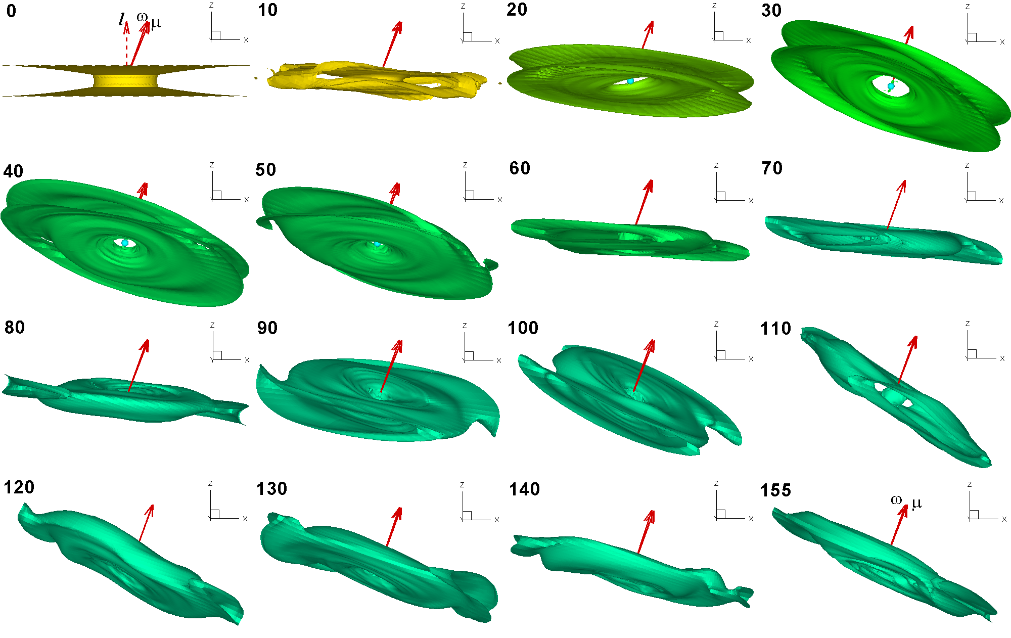
Figure 4: 3D views of the disc in Model A at different moments of time. The color background shows density levels which vary from $\rho=0.75-1.5$ in the top row of panels, to $\rho=0.23-0.54$ in three bottom rows of panels.

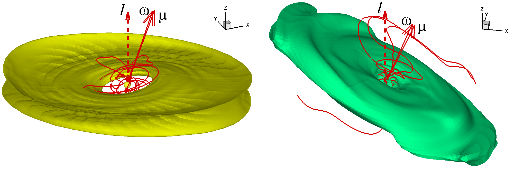
Figure 5: 3D views of the disc in Model A at moments $t=18$ (left) and $t=120$ (right), respectively. The color background shows the density levels. Lines are sample magnetic field lines.

3.2 Code description and dimensionalization

The code. We solve the 3D MHD equations with a Godunov-type code in a reference frame rotating with the star, using the “cubed sphere” grid (Koldoba et al., 2002). We use the 8-waves Roe-type approximate Riemann’s solver analogous to that described by Ruy & Jones (1995). We split the magnetic field to that of the star and induced by currents in the disc and corona.

In this work, we use the entropy balance equation instead of the full energy equation because we do not expect shocks inside the simulation region.

Viscosity. The viscosity term is incorporated into the momentum equation with the $\alpha-$prescription for the viscosity coefficient $\nu\sim\alpha p$, where $p$ is pressure in the disc (Shakura & Sunyaev, 1973). The viscosity is nonzero only inside the disc, above a threshold density ($\rho_{v}=0.1\rho_{d}$, where $\rho_{d}$ is the density in the disc). We use $\alpha=0.02$ in all simulation runs. In reality, the disc is expected to be turbulent, where turbulence can be driven by the magneto-rotational instability (MRI, e.g., Balbus & Hawley 1991). However, these simulations are time-consuming.

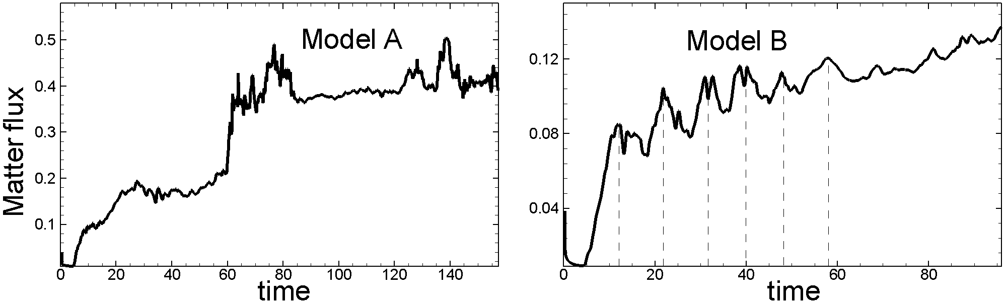
Figure 6: Temporal variation of matter flux $\dot{M}$ (in dimensionless units, see Tab. 2) at the surface of the star in models A and B (left and right panels, respectively). Dashed vertical lines in right-hand panel show peaks of $\dot{M}$ corresponding to moments of high tilt of the magnetic axis relative to the disc normal.

The grid consists of $N_{r}$ spheres. Each sphere represents an inflated cube with six sides. Each side has a $N\times N$ curvilinear grid, which represents a projection of the Cartesian grid onto the sphere. The whole grid consists of $6\times N_{r}\times N^{2}$ cells. We use the grid with $N_{r}=140$ and $N=61$. The MPI-parallelized code uses 28 layers in the radial direction and 6 layers for six sides of the inflated cube, with 168 layers total.

	CTTSs	White dwarfs	Neutron stars
$M_{\star}(M_{\odot})$	0.8	1	1.4
$R_{\star}$	$2R_{\odot}$	5000 km	10 km
$R_{0}$ (cm)	$4\times 10^{11}$	$1.4\times 10^{9}$	$2.9\times 10^{6}$
$P_{0}$	1.8 days	29 s	2.2 ms
$B_{\star 0}$ (G)	$10^{3}$	$10^{6}$	$10^{9}$
$B_{0}$ (G)	43	$4.3\times 10^{4}$	$4.3\times 10^{7}$
$\rho_{0}$ (g cm-3)	$7\times 10^{-12}$	$2\times 10^{-8}$	$2.8\times 10^{-5}$
$\dot{M}_{0}$ ($M_{\odot}$yr-1)	$2.8\times 10^{-7}$	$1.9\times 10^{-7}$	$2.9\times 10^{-8}$

Table 2: Sample reference values for three types of stars.

Dimensionalization. Equations are solved in dimensionless form. The dimensionless variables are determined as $\tilde{F}=F/F_{0}$, where $F$ are dimensional variables, while $F_{0}$ are their reference values. The reference value of distance $R_{0}$ is chosen such that the star has radius $R_{\star}=0.35R_{0}$. The reference velocity is the Keplerian velocity at $R_{0}$, $v_{0}=(GM_{\star}/R_{0})^{1/2}$. The reference time is $t_{0}=R_{0}/v_{0}$. The magnetic moment of the star: $\mu_{\star}=\mu^{\prime}B_{\star 0}R_{\star}^{3}$, where $B_{\star_{0}}$ is the reference surface magnetic field of the star at the magnetic equator and $\mu^{\prime}$ is dimensionless magnetic moment, which helps to vary the magnetic field of the star: $B_{\star}=\mu^{\prime}B_{\star_{0}}$. The reference magnetic field, $B_{0}$, is the value of the magnetic field at $r=R_{0}$: $B_{0}=B_{\star_{0}}(R_{\star}/R_{0})^{3}$. The reference density and pressure are $\rho_{0}=B_{0}^{2}/v_{0}^{2}$ and $p_{0}=\rho_{0}v_{0}^{2}$, respectively.

We take into account that $R_{0}=R_{\star}/0.35\approx 2.86R_{\star}$ and for convenience show distances in radii of the star. Also, we show time in periods of rotation at this radius, $P_{0}=2\pi R_{0}/v_{0}$. Below, we use dimensionless variables but drop tildes. The results of simulations can be applied to stars of different types. Table 2 shows sample reference values for different types of stars.

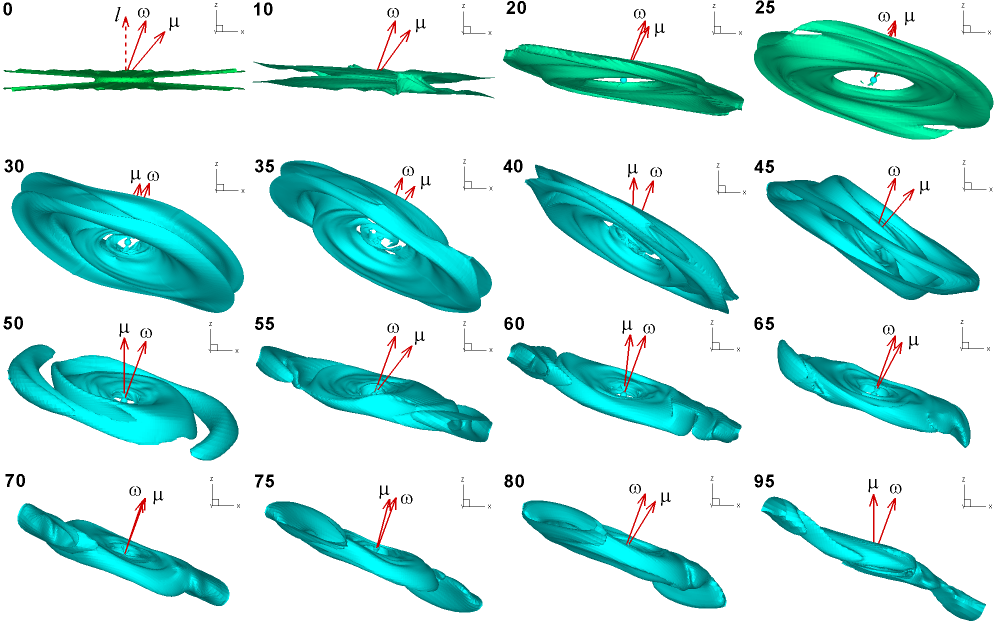
Figure 7: 3D views of the disc at different moments of time in Model B. The color background shows density levels which vary from $\rho=0.3-1.5$ in the top row of panels, to $\rho=0.15-0.2$ in three bottom rows of panels.

3.3 Set of models

We performed simulations at a variety of different parameters: different initial inclination angles of the rotational axis: $\beta=15^{\circ}$ and $20^{\circ}$; small and relatively large tilt angles of the dipole: $\theta=2^{\circ}$, $15^{\circ}$ and $20^{\circ}$; different values of the dipole moment: $\mu^{\prime}=1,0.5,0.3$; different values of the rotational period of the star, which varied from $P_{\star}=11.2$ to $P_{\star}=2.4$ . We also varied the initial position of the inner disc, $r_{\rm d_{i}n}$. Table 1 shows parameters of models.

Simulations show that in all models the inner disc was warped, then tilted, and became approximately flat. However, in some models, the normal to the tilted disc, ${\mbox{\boldmath$l$}}_{t}$ tends to align with the rotational axis of the star, and typical tilt angles are small, $\beta_{t}\approx 5^{\circ}-10^{\circ}$ (we call them aligned discs). In other models, the disc normal is tilted at a larger angle, $\beta_{t}\approx 30^{\circ}-40^{\circ}$ (we call them tilted discs). Comparisons of results at different sets of parameters showed that one of the main parameters is the initial position of the inner disc, $r_{\rm in}$. When we place the inner disc at larger distances, $r_{\rm in}=8.6$, we obtain only slightly tilted (aligned) discs. In the opposite case, $r_{\rm in}=5.7$, we obtain discs with larger tilts. Another important parameter is the corotation radius, $r_{c}$: at smaller values of this parameter (faster rotating stars) we obtain discs with larger tilts. Below, in Sec. 4 and 5, we consider two groups of models corresponding to two values of $r_{\rm in}$, and different values of $r_{c}$.

4 Models of aligned or slightly tilted discs (A, B, A1, B1, C)

In several models, we placed the inner radius of the disc at a relatively large distance from the star, $r_{\rm in}=8.6$. We considered two main models, A and B. In both models, the rotational axis of the star is tilted by $\beta=20^{\circ}$, while the tilt angles of the magnetosphere are different: $\theta=2^{\circ}$ in Model A and $\theta=20^{\circ}$ in Model B. In Model A, we took a disc of higher mass, while in Model B the disc has three times lower mass. In these models, we took the corotation radius $r_{c}=14.3$ which corresponds to a slow rotation of the star. We also considered three supplement models. Models A1 and B1 are identical to models A and B, but the disc mass is $\sim 3$ times lower/ higher, respectively. Model C is identical to Model A, but a star rotates more rapidly: $r_{c}=8.6$.

4.1 Accretion onto a star with a tilted rotational axis: $\beta=20^{\circ}$, $\theta=2^{\circ}$ (Model A)

In this model, we test the main new feature - how the inner disc evolves in the case when the rotational axis of the star is tilted about the rotational axis of the disc, while the magnetic axis is almost aligned.

We observed that the disc initially moved towards the star and was stopped by the magnetosphere at the distance $r_{m}$ where matter pressure in the disc equals the magnetic pressure of the magnetosphere (Pringle and Rees, 1972), that is where the modified plasma parameter $\beta_{1}=8\pi(p+\rho v_{\phi}^{2})/B^{2}=1$. At this distance, matter started flowing to the star in funnel streams (or in unstable tongues, e.g., Kulkarni & Romanova 2008). We used the condition $\beta_{1}=1$ in the equatorial plane to find the magnetospheric radius. This radius slightly varies in time due to variability in accretion rate. The time-averaged value is $\bar{r}_{m}\approx 3.4$. The top right panel of Fig. 2 shows the close view of matter flow near the star and $\beta_{1}=1$ line. Top middle panels of the same figure show $x^{\prime}z^{\prime}-$slices of density distribution and poloidal field lines at $t=15$ and $20$. One can see that the field lines inflate and become non-dipolar in most of the simulations region, excluding the inner parts of the disc, where the modified dipole can be seen (see the right-hand panel of the same figure).

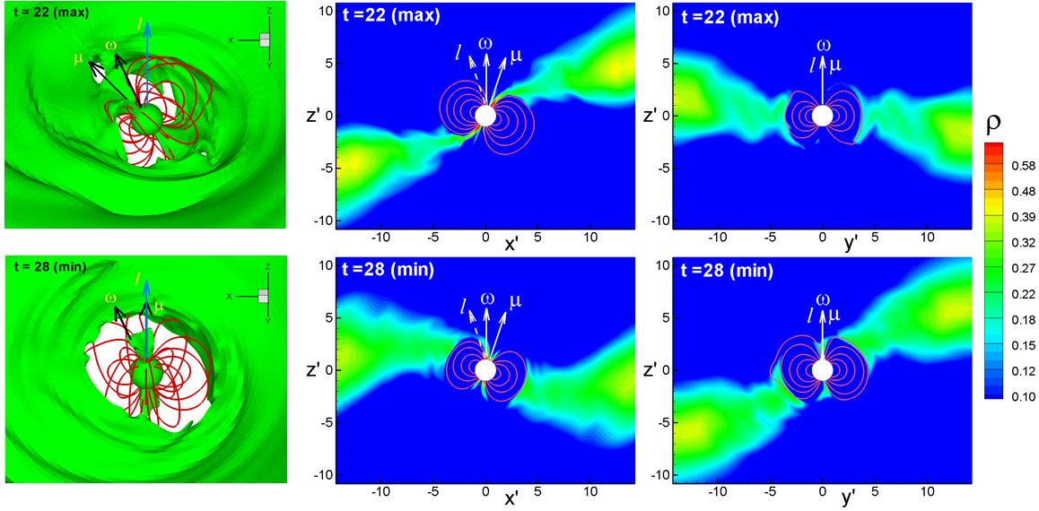
Figure 8: Left panels: 3D views of the inner disc during the episodes of the local maximum (top) and minimum (bottom) accretion rates in Model B at moments $t=22$ and $t=28$, respectively. The color background shows one of density levels. Lines are sample field lines. Middle and right panels: $x^{\prime}z^{\prime}$ and $y^{\prime}z^{\prime}$ slices of density distribution and sample field lines corresponding to the same moments in time.

The magnetic force and warping torque rapidly decrease with the distance from the star (see Eq. 4 for torque), and therefore they act mainly in the proximity of the disc-magnetosphere boundary. However, we see that a significant part of the disc becomes tilted. We suggest that information about the inner warp propagates to larger distances in the form of bending waves. According to Papaloizou & Pringle (1983) and Papaloizou & Lin (1995), the disc may be either in the diffusive regime (if $h(r)/r<\alpha_{2}$), or in wave regime (if $h(r)/r>\alpha_{2}$). In our simulations $\alpha_{2}\approx 0.02$, the ratio $h(r)/r\approx 0.1-0.15$, $\alpha_{2}<h(r)/r$, and the disc is in the wave regime.

Fig. 4 shows 3D views of the disc at different times in Model A. We observed that the inner parts of the disc were warped, precessed, and tilted under the influence of the magnetic force, as predicted by the theory (see Sec. 2). Initially, at $t=10-20$, the warp formed in the inner parts of the disc. Later, at $t>20$, larger parts of the disc become warped and tilted. Subsequently, the significant part of the inner disc becomes tilted and almost flat. Fig. 4 also shows that the disc can be split into two parts: the inner part, which is almost flat and has the same tilt, and the outer part with a different tilt (see, e.g., panels at $t=120,130$ and $140$). We call the inner part the “tilted disc”. Its time-averaged radius is $r_{t}\approx 24.3$ (in stellar radii) or $r_{t}/{\bar{r}}_{m}\approx 7.3$ in magnetospheric radii (see Tab. 1).

The disc slowly precesses about the rotational axis of the star. The rate of precession, $\Omega_{p}(r)$ (see Eq. 7) depends on a number of factors, including the factor $f$ which characterizes the dielectric property of the disc. If only the time-varying component is screened, $f=0$, we obtain a factor $\sim\sin{\theta}\approx 0.035$. However, we observed comparable rates of precession in models with $\theta=2^{\circ}$ and larger values of $\theta$. We suggest that we have some intermediate situation, in which $0<f<1$.

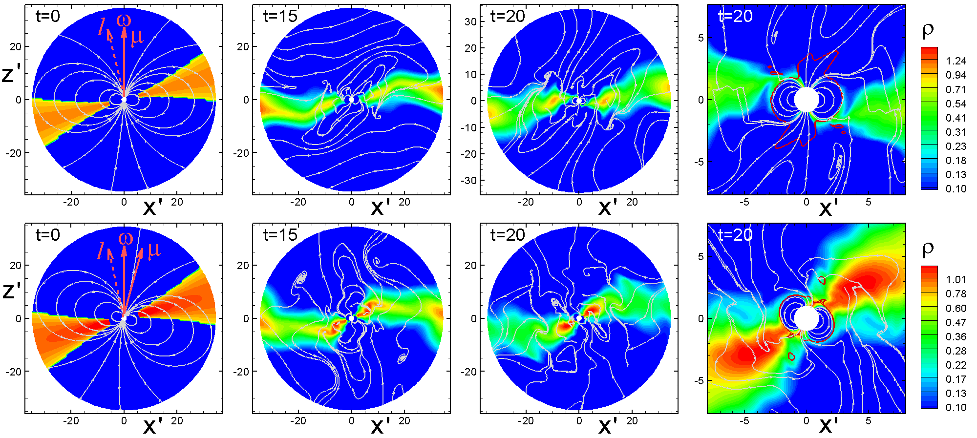
Figure 9: $x^{\prime}z^{\prime}-$slices of density distribution in models D and F (top and bottom panels, respectively) at $t=0$, $t=15$, and $t=20$. Top and bottom right panels show close view of matter flow near the magnetosphere at $t=20$. White lines show sample poloidal magnetic field lines. Red lines shows the $\beta_{1}=1$ line.

We observed that after a few periods of stellar rotation (approximately after $t=70$, see Fig. 4), the disc starts tilting towards the equatorial plane of the star, so that the disc normal becomes almost parallel to the angular velocity of the star, $\omega$. There is still some tilt, but it is small, $\beta_{t}\lesssim 5^{\circ}-10^{\circ}$. We discuss possible mechanisms of the disc alignment in Sec. 6. Fig. 5 shows typical initial and final states of the disc evolution.

The left-hand panel of Fig. 6 shows the accretion rate onto the star. We observed persistent accretion during 160 rotations (Keplerian periods at $r=1/0.35\approx 2.86$), which is approximately 14 periods of stellar rotation. Initially, the accretion rate increases due to the inward flow of the disc matter from the initial radius $r_{i}=8.6$ to the radius, where the disc is stopped by the magnetosphere, at $\bar{r}_{m}\approx 3.4$. Later, at $20\lesssim t\lesssim 60$, matter accrets in two funnel streams, and accretion is quasi-stationary. At $t\gtrsim 60$, more matter arrived to the inner disc, and accretion switched to the unstable regime where matter penetrates through the magnetosphere in the unstable “tongues” (e.g., Romanova et al. 2008; Kulkarni & Romanova 2008, 2009). The onset of the unstable regime depends on the effective gravity (the sum of the gravitational and centrifugal potential), and therefore depends on the ratio $\bar{r}_{m}/r_{c}$. According to Blinova et al. (2016), accretion becomes unstable, if $r_{m}/r_{c}\lesssim 0.71$ (in their set of simulations, where the magnetic axis is tilted by $\theta=5^{\circ}$).

In our model the star rotates slowly compared with the inner disc, $\bar{r}_{m}/r_{c}\approx 0.24$. However, accretion is stable up to $t\approx 60$, and becomes unstable at $t>60$. At $t<60$, the magnetospheric radius was only slightly larger during stable regime. We conclude that in the case of the tilted rotational axis the unstable regime is less favorable compared with the aligned case considered by Blinova et al. (2016).

4.2 Both the rotational and magnetic axes are tilted: $\beta=20^{\circ}$, $\theta=20^{\circ}$ (Model B)

Next, we consider the model where both axes are misaligned. In this model, the mass of the disc is $\sim 3$ times smaller than that in Model A. The bottom panels of Fig. 2 show that we start from a thin disc, which expands and becomes comparable in thickness with the disc in Model A. The density in the disc is $\sim 3$ times smaller than in Model B.

The overall evolution of the disc is similar to that in Model A. Namely, initially, the inner parts of the disc are warped, then tilted, and precess about the rotational axis of the star. After 1-2 periods of precession the disc settles near the rotational equatorial plane of the star, and the disc normal has a small tilt angle, $\beta_{t}\sim 5^{\circ}-10^{\circ}$ relative to the rotational axis of the star (see Fig. 7).

In this model, the disc is of the lower density and as a result the time-averaged radius of the magnetosphere $\bar{r}_{m}\approx 4$ is larger than in Model A ($\bar{r}_{m}\approx 3.4$). The radius of the tilted disc is slightly smaller than that in Model A: $r_{t}\approx 21.8$. The disc is mainly flat, but, compared with Model A, there is an additional wavy structure connected with rotation of the magnetic axis about the rotational axis of the star. The alignment of the inner disc normal with the rotational axis of the star occurs faster than in Model A. This may be due to the lower density in the disc. Namely, in Eq. 5 the warping rate $\Gamma_{w}$ is inversely proportional to the surface density $\Sigma$, and this may explain the faster variation of the tilt angle in Model B.

We calculated the accretion rate onto the star. We note that the magnetic moment of the star is tilted about the disc normal at different angles. During one rotational period, the position of the magnetic axis relative to the initial disc axis varies between strongly tilted ($\chi=\beta+\theta=40^{\circ}$) and the aligned one ($\chi=\theta-\beta=0^{\circ}$). In the former case, the accretion through funnel streams is more favorable due to the high tilt of the magnetosphere towards the disc. This leads to the variation of the accretion rate at the surface of the star. The right panel of Fig. 6 shows several maxima and minima which correspond to different tilts of the magnetic axis relative to the disc.

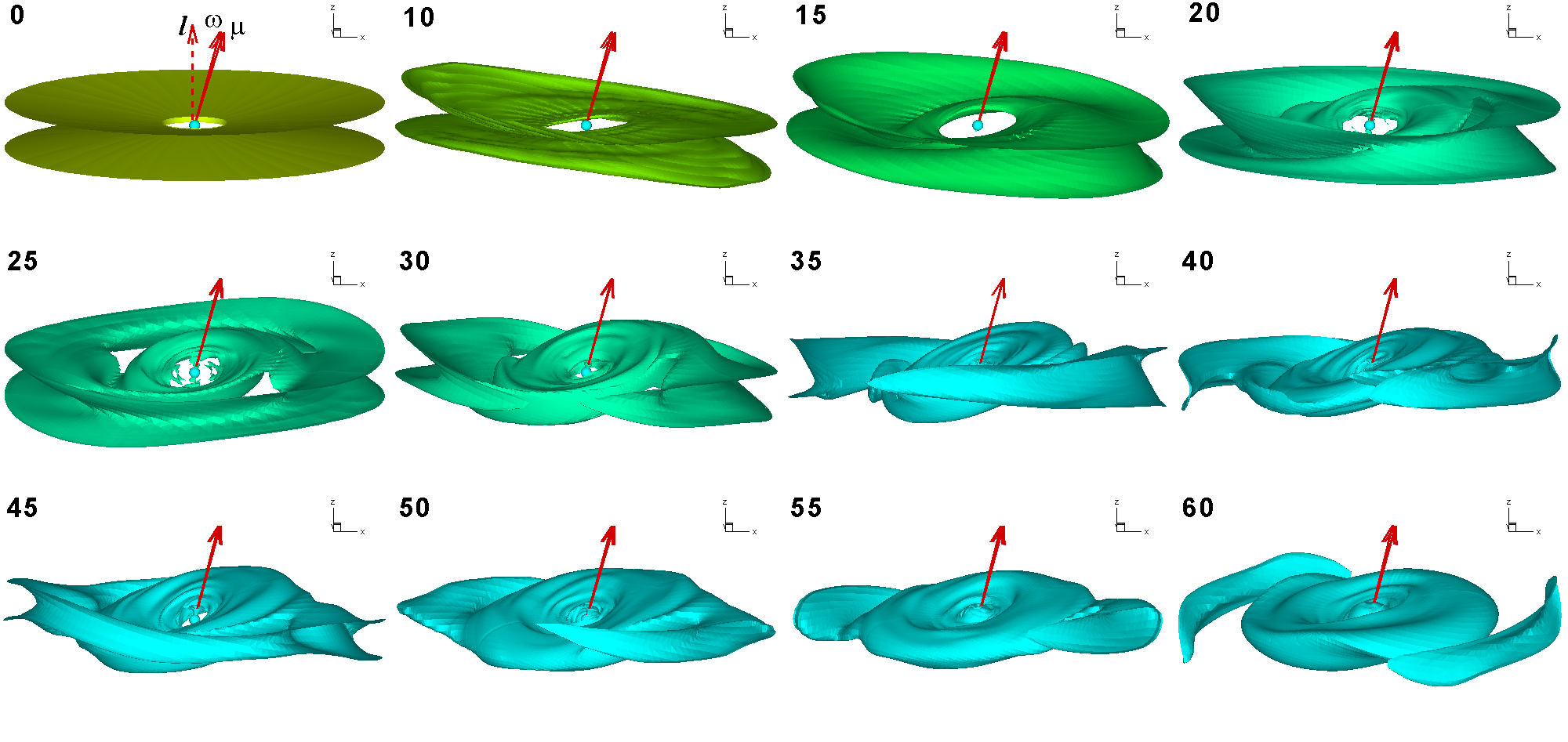
Figure 10: 3D views of the disc in Model D at different moments of time. The color background shows density levels which vary from $\rho=0.3-1.5$ in the top row of panels, to $\rho=0.15-0.2$ in two bottom rows of panels.

We chose two moments in time corresponding to the maximum ($t=22$) and minimum ($t=28$) of the accretion rate and checked the position of the magnetosphere and the nature of the matter flow at these moments. The top left panel of Fig. 8 shows that at $t=22$, the magnetic axis $\mu$ is strongly tilted about the rotational axis of the inner disc, and two funnel streams are formed. The bottom left panel shows that at $t=28$ the magnetic axis is almost perpendicular to the disc, accretion in funnels is less favorable, and only weak funnel streams formed. Middle and right panels of Fig. 8 show the $x^{\prime}z^{\prime}$ and $y^{\prime}z^{\prime}-$slices of density distribution during high and low tilts of the magnetic axis. One can see that funnels form more efficiently during episodes of higher tilt of the magnetosphere.

The amplitudes of maxima in the curve for the accretion rate are larger initially when the disc normal had a higher tilt about the rotational axis of the star. Later, when the disc becomes almost aligned, the tilt of the magnetic axis only slightly varied about the normal to the disc and the amplitudes of maxima become smaller.

This model shows that in the case when both axes are misaligned, the main result is similar to that in the case of the aligned dipole: the disc tends to be in the rotational equatorial plane of the star. We consider possible explanations of the disc alignment in Sec. 6.

4.3 Dependence on the disc mass and rotation rate (models A1, B1, C)

The supplement models A1 and B1 are identical to models A and B, but the disc mass is $\sim 3$ times larger/smaller, respectively. Simulations have shown the same main result: the tilted disc settled approximately in the equatorial plane of the star such that the normal to the inner disc is tilted only at a small angle relative to the rotational axis of the star. The accretion rate is 3 times smaller/larger, respectively. In Model B1, the variability in the matter flux, associated with different tilts of the magnetic axis has also been observed. Episodes of unstable accretion were observed in Model B1, where the magnetospheric radius is smaller. These models have shown that result does not depend on the factor of 3 variations in the disc mass.

We also tested a model similar to Model A, but for a faster rotating star, $r_{c}=8.6$, $P_{\star}=5.2$ (Model C). We observed the formation of the inner tilted disc similar to that in Model A. However, the normal to the inner disc is tilted at a slightly larger angle: $\beta_{n}\sim 15^{\circ}-20^{\circ}$. We suggest that there may be a dependence of the tilt on the rotation rate of the star. We note that the physics of the disc-magnetosphere interaction often depends on the ratio $r_{m}/r_{c}$ (e.g., Ghosh & Lamb 1978; Blinova et al. 2016). This ratio $\bar{r}_{m}/r_{c}\approx 0.39$ is larger in this model versus models A and B: $\bar{r}_{m}/r_{c}\approx 0.24,0.28$ (see Tab. 1). We further investigate this issue in Sec. 5.

5 Models of tilted discs (D, E, F)

In this section, we consider discs that show a large tilt angle at the end of simulations. In these models, we placed the initial radius of the disc closer to the star, at $r_{\rm in}=5.7$ (versus 8.6 in the above models) and therefore a stronger dipole magnetic field threads the disc. We also took faster rotating stars. We observed qualitatively different result: the normal to the inner disc was systematically tilted at a large angle away from the rotational axis of the star.

In these models, the tilt of the rotational axis is $\beta=15^{\circ}$, and tilts of the magnetic axes are $\theta=2^{\circ}$ or $15^{\circ}$. The corotation radius $r_{c}=8.6$ or $r_{c}=5.1$ which correspond to periods of the star $P_{\star}=5.2$ and $P_{\star}=2.4$ We took smaller values of the magnetic moment: $\mu^{\prime}=0.5$ and $0.3$. See Tab. 1 for all set of parameters. We show sample results for these models.

Three left panels of Fig. 9 show $x^{\prime}z^{\prime}-$slices of the initial density distribution and sample magnetic field lines in models D and F at times $t=0,15,20$. Right panels show close view of the magnetospheric accretion at $t=20$. Note that the magnetospheric radii are smaller than in models $\rm A-C$: $\bar{r}_{m}=2.9$ and $2.1$ in models D and F, respectively.

Fig. 10 shows 3D views of the disc in Model D. One can see that the inner disc becomes warped, then tilted, and the inner disc seems to be disconnected from the outer parts of the disc. The radius of the tilted disc $r_{t}\approx 19$ and its normal vector is tilted away from the rotational axis of the star at an angle $\beta_{t}\approx 30^{\circ}-40^{\circ}$, which is much larger than that in models $\rm A-C$. We observed very slow precession in this model.

In two other models (E and F) similar tilted discs were formed, with tilt angles, $\beta_{t}\approx 30^{\circ}-40^{\circ}$, and tilt radii $r_{t}=19.4$ and $17.7$. Discs in models E and F precess with usual rates of 1-1.5 precession periods per simulation run. In Model D the precession is very slow.

The magnetic field lines wrap due to the rotation of the inner disc and rotation of the star. The right-hand panel of Fig. 12 shows the field lines in Model D during a relatively early time of evolution ($t=30$). One can see that the field lines wrap about the disc normal because the disc rotates more rapidly than the star. However, wrapping about the rotational axis of the star was also observed. On the longer time scale, the field lines form a magnetic tower about the rotational axis of the star.

Fig. 11 shows matter fluxes in these models. In model F, where $\theta=15^{\circ}$, one of the variabilities is connected with different tilts of the magnetic axis relative to the disc (like in Model B, see Fig. 6). The quasi-period of variability approximately equals to the period of the star, $P_{\star}=2.4$). Variabilities in models E and D and the flaring component of variability in Model F are connected with non-stationary and/or unstable accretion.

One of the main differences between this set of models and the earlier discussed set of models ($\rm A-C$) is that the inner disc was initially closer to the star, and stronger dipole field threads the disc. Therefore, the role of the dipole component (which helps to tilt the disc) is more significant. Namely, in Eq. 3, the dipole components $B_{\phi}$ and $B_{z}$ are important in providing the force $F_{z}(r)$ and warping torque $N_{w}(r)$ which persistently tilt the disc away from the equatorial plane of the star. On the other hand, we noticed in the test Model C and current models, that the disc is more tilted when the star rotates more rapidly. We calculated the ratios $\bar{r}_{m}/r_{c}$ and noticed that they are larger than in models $\rm{A-C}$ (see Tab. 1). We discuss possible reasons which lead to alignment or tilting of the disc in the next section.

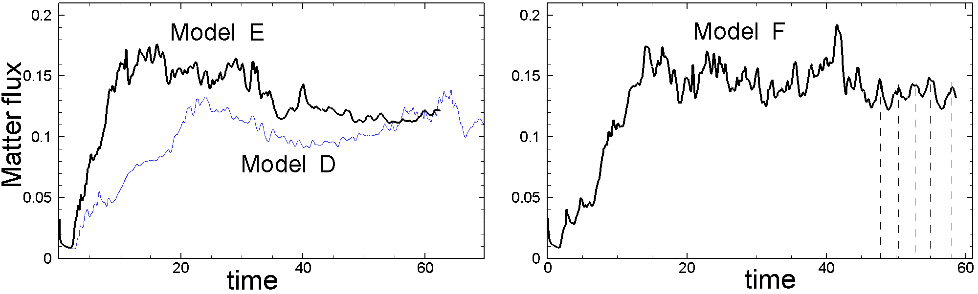
Figure 11: Temporal variation of matter flux $\dot{M}$ at the surface of the star. Left-hand panel shows $\dot{M}$ in models D (blue color) and E, and right-hand panel for Model F. Vertical dashed lines show maxima corresponding to high tilt of the magnetic axis towards the inner disc.

6 Mechanisms of disc alignment and tilting

In our models the disk breaks up into two parts. The tilt of the inner disc, $\beta_{t}$, is different in different models Below we discuss possible mechanisms explaining different tilts of the inner disc.

6.1 Mechanisms of disc alignment

In models $\rm{A-C}$ the normal to the tilted disc tends to align with the rotational axis of the star. Below we consider two possible explanations for this phenomenon.

In our models, the magnetic field lines are wrapped due to the differential rotation of their foot-points connecting the star and the disc. The inner disc rotates more rapidly than the magnetosphere of the star, and the field lines are wrapped about the normal to the inner disc and expand forming a local magnetic tower. The inner disc changes its tilt and the tower changes its direction. At the same time, a star rotates and the field lines wrap about the rotational axis of the star. On a long time scale and larger spatial scales, the magnetic tower becomes more and more symmetric about the rotational axis of the star. Left-hand panel of Fig. 12 shows the magnetic tower observed in Model B at $t=62$. Note that at this time the normal to the inner disc has a small angle relative to the rotational axis of the star, which makes the tower more symmetric.

The right-hand panel of Fig. 12 shows the tower in Model D, where the disc normal is tilted at a large angle and at the earlier moment in time, $t=30$. One can see that near the disc the field lines wrap about the disc normal, while at larger distances the wrapping about the stellar rotational axis is seen. In reality, both components of the wrapped field are present in all models. The azimuthal component of the field above and below the disc can be presented as a sum of the field wrapped about the disc normal (marked with letter $d$) and stellar rotational axis (marked with letter $s$): $B_{\phi}^{top}=B_{\phi}^{d}+B_{\phi}^{s,top}$ and $B_{\phi}^{bot}=B_{\phi}^{d}+B_{\phi}^{s,bot}$. The disc components of the field are approximately equal. However, the stellar component is expected to be stronger near parts of the disc that are closer to the rotational axis of the star. In the right panel of Fig. 12, the field is stronger near the top right and bottom left parts of the tilted disc. Therefore, there is the magnetic force acting on the disc which is the difference between magnetic pressure at the top and bottom sides of the disc:

$$F_{z}(r,\phi)={1\over 8\pi}\left[(B_{\phi}^{d}+B_{\phi}^{s,top})^{2}-(B_{\phi}^{d}+B_{\phi}^{s,bot})^{2}\right].$$ (8)

The corresponding torque acts to align the normal to the disc with the rotational axis of the star. This torque acts in the direction opposite to the warping torque. We suggest that this may be a possible mechanism for the disc alignment in models $\rm A-C$. Note that in Eq. 8, the magnetic pressure results from the winding of the field lines, threading the disc. Note that in Eq. 3 for magnetic force providing the warping torque, the azimuthal field associated with the inflated field is taken to be equal on the top and bottom sides of the disc, and the main asymmetry is connected with the $B_{\phi}-$component of the dipole field. We suggest that in models $\rm A-C$ (where the inner disc was located at a larger distance from the star), the dipole component has been relatively weak, and the alignment torque dominates over warping torque. In opposite, in models D, E, F (where the inner disc was closer to the star), the dipole component is stronger, and warping torque dominates.

To investigate further this issue, we calculated the poloidal current $J_{p}\sim rB_{\phi}$ and observed that the current flows above and below the disc, and it is almost symmetric about the disc plane (see left panel of Fig. 13). We draw a line perpendicular to the disc (see white dashed line in the left panel) and calculated the value of ${B_{\phi}}^{2}$ along this line. The right panel of Fig. 13 shows that the magnetic pressure distribution is not perfectly symmetric about the plane of the disc, and the pressure difference provides the magnetic force, which may be responsible for the tilting of the disc. Note that the magnetic pressure dominates over the matter pressure in the corona above and below the inner parts of the disc. Middle panel of Fig. 13 shows the distribution of the plasma parameter $\beta=8\pi p/B^{2}$. One can see that $\beta<1$ in the corona above and below the disc at $r\lesssim 11$ (see darker green regions). There is also a region where the matter pressure dominates, but the magnetic pressure is still significant and can contribute to the dynamics of the disc (see the light-green region at $r\lesssim 14$ where $\beta<10$). The sizes of these regions vary in time and also from model to model. However, they are always a few times larger than the magnetospheric radius $r_{m}$. We suggest that this magnetic force and corresponding torque may drive the tilted discs towards the aligned position.

Another possible explanation for the disc alignment is the magnetic Bardeen-Petterson effect (see Sec. 2.3), where the viscous and precession torques push the inner disc to be aligned with the equatorial plane of the star. Typically, we observe 1-2 periods of precession. This time may be too short for the development of the Bardeen-Petterson effect. In the case of compact stars, the time scale to achieve the Bardeen-Petterson alignment is different in different models and varies from a few precession time scales (evaluated at $R_{\rm BP}$) up to $10-100$ (e.g., Pringle 1992).

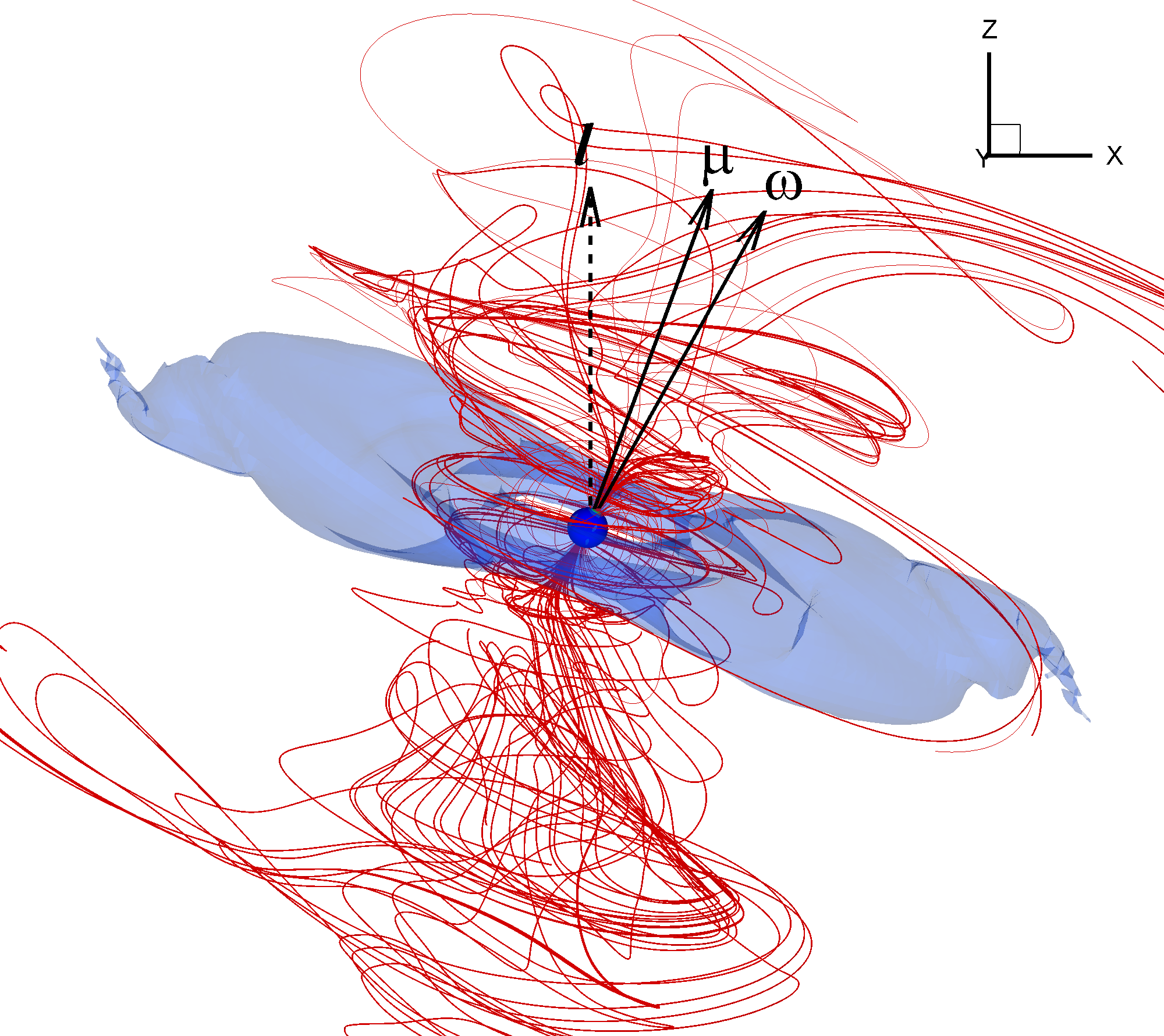
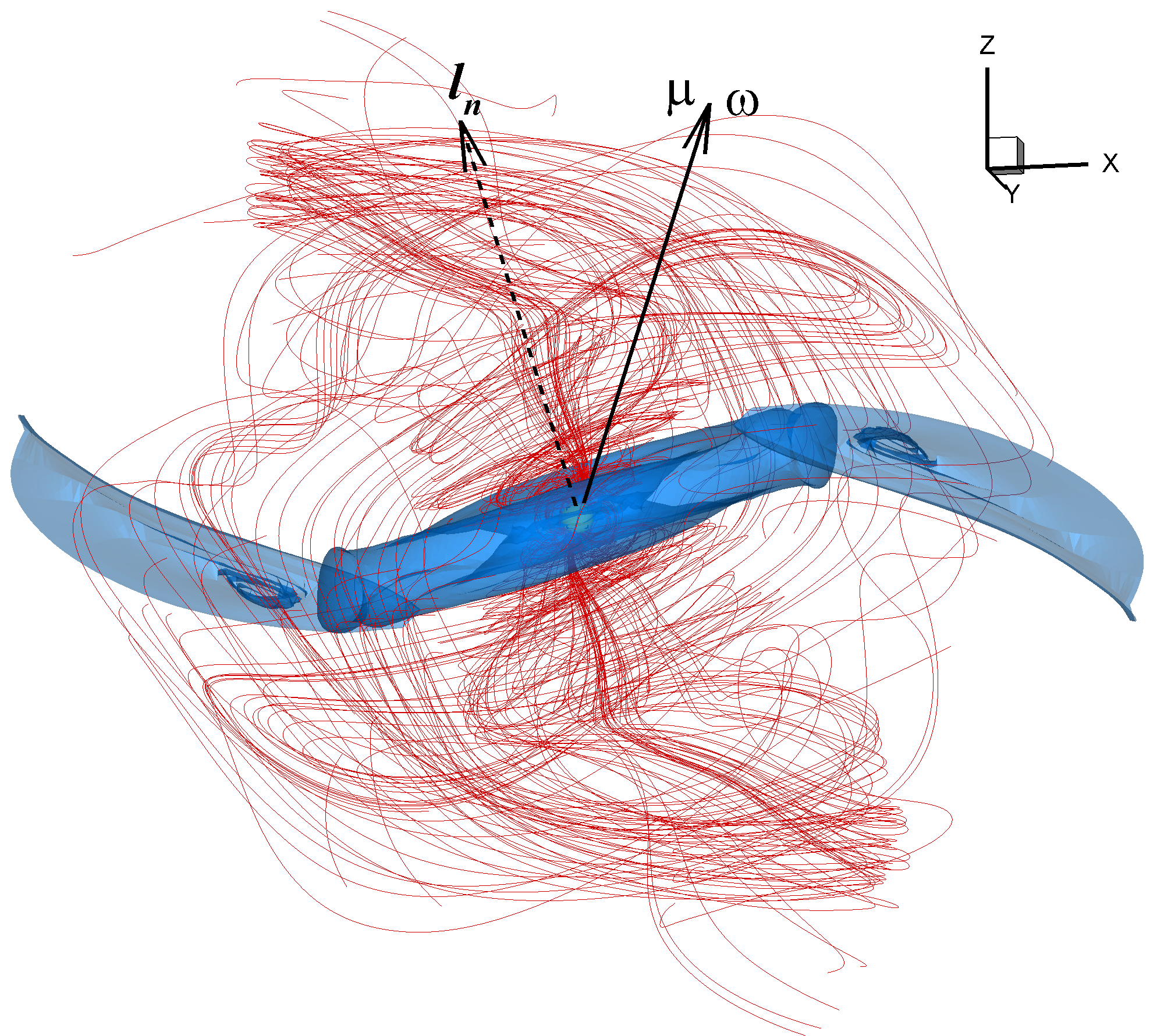
Figure 12: Left panel: Figure demonstrates inflation of the magnetic field lines in Model B at $t=62$. The color background shows one of the density levels, $\rho=0.17$. Lines are sample magnetic field lines. Right panel: Same but for Model D at $t=30$ and for density level $\rho=0.3$.

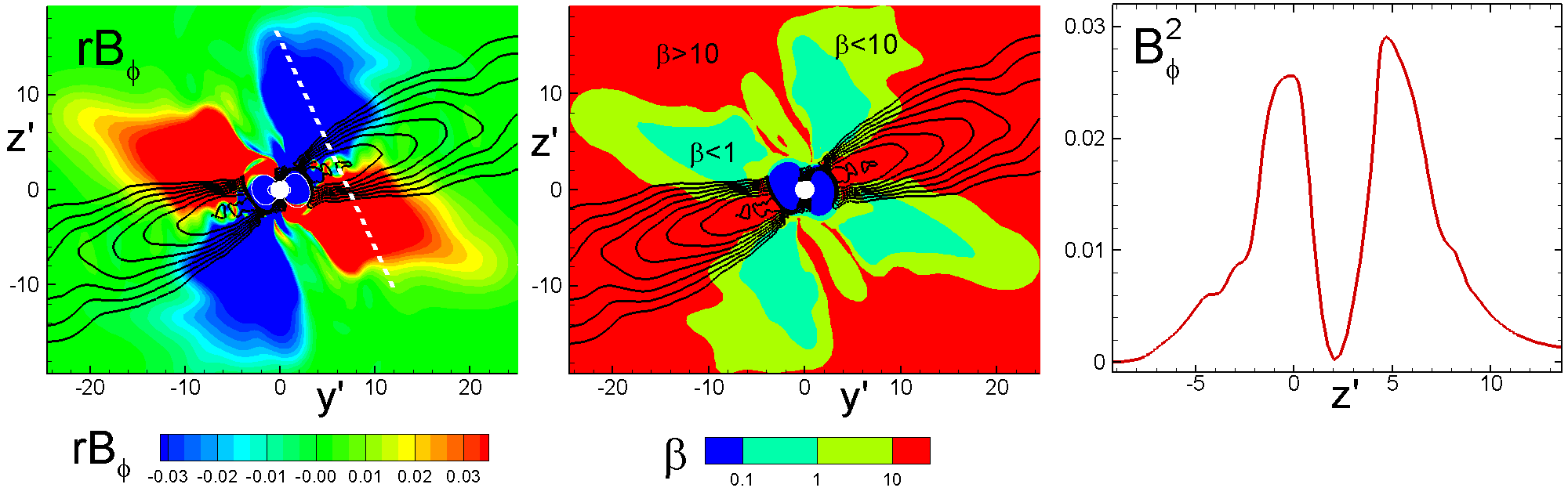
Figure 13: Left panel: the distribution of the poloidal current $rB_{\phi}$ in the slice $y^{\prime}z^{\prime}$ in Model A at $t=50$. Middle panel: the distribution of the plasma parameter $\beta=8\pi p/B^{2}$. We show $\beta$ in three regions, separated by values $\beta=0.1,1,10$. Right panel: the distribution of the $B_{\phi}^{2}$ along the dashed line shown in the left panel.

6.2 Mechanisms of tilting

The warping instability discussed in Sec. 2.1 always acts to tilt the inner disc normal away from the rotational axis of the star (see, e.g., Lai et al. 2011). The warping torque operates at distances comparable with the magnetospheric radius. It is stronger in models D, E, F where the inner disc is closer to the star, and a stronger dipole field threads the inner disc.

On the other hand, the winding of the field lines about the stellar rotational axis provides a force that acts to align the disc. If a star rotates slowly (as in models A, A1, B, B1) then the role of winding is more significant, because there is a larger difference between angular velocities of the star and the disc. In these models, we observe almost aligned discs. If a star rotates more rapidly (like in models $\rm C-F$) then the role of the force associated with winding is less important, and the warping force dominates.

7 Discussion and conclusions

We performed three-dimensional MHD simulations of accretion onto a rotating magnetized star where both the magnetic and rotational axes of the star are tilted about the rotational axis of the disc.

7.1 Summary: Dependence on parameters

Our simulations are exploratory and are aimed at understanding the matter flow near the magnetized star where both the magnetic and rotational axes are tilted. We varied different parameters (see Tab. 1). In addition to evident parameters, such as the magnetic moment, $\mu^{\prime}$, or period of the star, $P_{\star}$, we also varied the initial position of the inner disc, $r_{\rm in}$, and observed strong dependence on this parameter. Below, we conclude about dependence on different parameters.

• $r_{\rm in}-$the initial positions of the inner disc. We observed that in models $\rm A-C$, where the inner disc is located at a larger radius, $r_{\rm in}=8.6R_{\star}$, the final tilt angle of the disc is smaller, $\beta_{t}\sim 5^{\circ}-10^{\circ}$, compared with models D, E, F, where the disc is located closer to the star, $r_{\rm in}=5.7R_{\star}$, and the tilt of the disc is larger, $\beta_{t}\sim 30^{\circ}-40^{\circ}$.

• $\beta-$initial tilt of the rotational axis of the star relative to the disc normal. We did not see a difference between results in models with $\beta=20^{\circ}$ and $\beta=15^{\circ}$.

• $\theta-$the tilt of the magnetic axis relative to the rotational axis. There is almost no difference in results for models with almost aligned ($\theta=2^{\circ}$) and misaligned ($\theta=20^{\circ}$, $\theta=15^{\circ}$) cases. The main difference is that in models with larger $\theta$, we observed variability in the matter flux, which is associated with different tilt angles between the magnetosphere and the disc.

• $r_{c}-$the corotation radius and $P_{\star}-$period of the star. In models D, E, F, stars rotate more rapidly than in models A, A1, B, and B1, and this could be a factor that leads to larger tilts of discs in these models. We suggest that at smaller values of $r_{c}$ and larger values of $\bar{r}_{m}/r_{c}$, the difference in angular velocities between the star and the disc is smaller, and winding of the field lines (which helps to align the disc) is less efficient.

• $\mu^{\prime}-$the magnetic moment of the star: $\mu^{\prime}=1,0.5,0.3$. We observed that the size of the tilted disc, $r_{t}$, decreases with $\mu^{\prime}$. This is an expected result, because at smaller values of $\mu^{\prime}$ the magnetic force is smaller.

• $M_{d}-$mass of the disc. In test simulations with $\sim 3$ times lower disc mass (models B and A1) we observed similar parameters for tilted discs. However, discs were warped and tilted more rapidly. This may be explained by the fact that the warping rate has an inverse dependence on the surface density: $\Gamma_{w}\sim\Sigma^{-1}$ (see Eq. 5).

• $\tau_{\rm sim}-$duration of simulations. Originally, we included into consideration only the longest simulation runs (models A and B) which show almost aligned discs. However, later, we realized that models D, E, F are also valuable because they show persistent tilts. In these models, the time measured in Keplerian rotations at, $\tau_{\rm sim}/P_{0}$, is shorter. However, time measured in periods of stellar rotation, $\tau_{\rm sim}/P_{\star}$, is comparable or longer than in models A and B. The rotation of the star is an important factor in winding the field lines and may influence the physics of the process.

7.2 Conclusions

1. Simulations show that the disc-magnetosphere interaction led to the formation of tilted, almost flat discs in all models. However, discs may have different tilts. The tilt angles of the disc normal relative to the rotational axis of the star are small ($\beta_{t}\sim 5^{\circ}-10^{\circ}$) in models, where the star rotates slowly and where initially the disc is located at a larger distance from the star so that a weaker dipole field threads the disc. When stars rotate more rapidly and the inner disc is located closer to the star (so that the stronger dipole field threads the disc), the tilt angles are larger ($\beta_{t}\sim 30^{\circ}-40^{\circ}$).

2. The sizes of the tilted discs systematically increase with the strength of the magnetic field, $\mu^{\prime}$. They vary in the range of $r_{t}\approx 17.7-24.3$ if measured in stellar radii. They are typically $\sim 5.3-8.6$ times larger than the magnetospheric radii.

3. Tilted discs slowly precess in most of models. The time scale of precession is $\tau_{p}\sim 50P_{0}$, where $P_{0}$ is the period of Keplerian rotation at $r=R_{0}\approx 2.86R_{\star}$.

4. In models with a significant tilt of the magnetic axis ($\theta=20^{\circ}$ and $15^{\circ}$), the accretion rate onto the star varied due to the different positions of the magnetospheric axis about the inner disc. Accretion is more favorable when the magnetic axis is strongly tilted towards the disc plane. The quasi-period of variations is close to the period of the star.

5. Accretion in the unstable regime has been observed in models with higher-mass discs and smaller tilts of the magnetosphere.

Overall, tilted discs are expected to form around magnetized stars with the tilted rotational axis. However, the tilt angle and other parameters of the disc depend on the properties of the star and details of the disc-magnetosphere interaction.

7.3 Application to different stars

Tilted precessing discs are expected in different types of accreting magnetized stars.

1. The signs of tilted discs are observed in cataclysmic variables (CVs). They are often observed as temporary features. The origin of the tilt is not well understood (see, e.g., Montgomery & Martin 2010). We suggest that tilted discs may result from the action of the magnetic field, as observed in our models, where the disc is expected to be tilted as long as the dipole magnetic field partly threads the disc. Note that the inflated field lines may drive outflows or jets from the disc-magnetosphere boundary. The orientation of the magnetic tower may be important for determining the direction of such outflows (e.g., Lovelace et al. 2014).

2. In another example, accreting millisecond pulsars in X-ray binaries show a variety of quasi-periodic oscillations (QPOs) (see, e.g., van der Klis 2006). We suggest that the low-frequency QPOs can be connected with the precession of tilted discs, driven by the magnetic forces (see also Lai 1999).

3. The long-term variabilities of unknown nature have been observed in classical T Tauri stars and Ae Herbig stars (e.g., Artemenko et al. 2010; Rigon et al. 2017). Some of them may be connected with tilted precessing discs.

8 Data availability

3D and 2D plots shown in the paper were produced using data obtained in 3D MHD simulations. These data will be shared on reasonable request to the corresponding author.

References

- Aly (1980) Aly, J.J. 1980, A&A, 86, 192
- Balbus & Hawley (1991) Balbus, S.A. & Hawley, J. F. 1991, ApJ, 376, 214
- Artemenko et al. (2010) Artemenko, S. A., Grankin, K. N., Petrov, P. P. 2010, Astronomy Reports, 54, 163
- Bardeen & Petterson (1975) Bardeen, J.M. & Petterson, J.A. 1975, ApJ, 196, L65
- Bessolaz et al. (2008) Bessolaz N., Zanni C., Ferreira J., Keppens R., Bouvier J. 2008, A&A, 478, 155
- Blinova et al. (2016) Blinova, A. A., Romanova, M. M., Lovelace, R. V. E. 2016, MNRAS, 459, 2354
- Bouvier et al. (1999) Bouvier, J., Chelli, A., Allain, S., Carrasco, L., Costero, R., Cruz-Gonzalez, I., Dougados, C., Fernandez, M. et al. 1999, A&A, 349, 619
- Bouvier et al. (2007) Bouvier J., Alencar S. H. P., Harries T. J., Johns-Krull C. M., Romanova M. M., Protostars and Planets V, Eds. Reipurth B., Jewitt D., Keil K. (University of Arizona Press, Tucson, 2007) 479
- Donati et al. (2007) Donati, J.-F., Jardine, M. M., Gregory, S. G., et al., 2007, MNRAS 380, 1297
- Donati et al. (2010) Donati, J.-F., Skelly, M. B., Bouvier, J., Gregory, S. G., Grankin, K. N., Jardine, M. M., Hussain, G. A. J., Ménard, F. et al. 2010, MNRAS, 409, 1347
- Donati et al. (2011) Donati, J.-F., Bouvier, J., Walter, F. M., Gregory, S. G., Skelly, M. B., Hussain, G. A. J., Flaccomio, E., Argiroffi, C. et al. 2011, MNRAS, 412, 2454
- Dyda & Reynolds (2020) Dyda, S., & Reynolds, C. S. 2020, MNRAS, in press. arXiv:2008.12381v1
- Fateeva et al. (2016) Fateeva, A. M., Zhilkin, A. G., and Bisikalo, D. V. 2016, Astronomy Reports, 60, 87
- Foucart & Lai (2011) Foucart, F. & Lai, D. 2011, MNRAS, 412, 2799
- Fragile et al. (2007) Fragile, P.C., Blaes, O.M., Anninos, P., Salmonson, J.D. 2007, ApJ, 668, 417
- Ghosh & Lamb (1978) Ghosh, P., Lamb, F. K., 1978, ApJ, 223, L83
- Gregory (2011) Gregory, S. G. 2011, American Journal of Physics, 79, 461
- Hellier (2001) Hellier, C. 2001, Cataclysmic variable stars, (Springer, Berlin 2001)
- Ivanov & Illarionov (1997) Ivanov, P. B., & Illarionov, A. F. 1997, MNRAS, 285, 394
- Johns-Krull (2007) Johns-Krull C. M., 2007, ApJ, 664, 975
- Koldoba et al. (2002) Koldoba, A. V., Romanova, M. M., Ustyugova, G. V., Lovelace, R. V. E. 2002, ApJ, 576, L53
- Koldoba et al. (2008) Koldoba, A. V., Ustyugova, G. V., Romanova, M. M., Lovelace, R. V. E. 2008, MNRAS, 388, 357
- Krolik & Hawley (2015) Krolik, J. H., & Hawley, J. F. 2015, ApJ, ApJ, 806, 141
- Kulkarni & Romanova (2008) Kulkarni, A., & Romanova, M.M. 2008, ApJ, 386, 673
- Kulkarni & Romanova (2009) Kulkarni, A., & Romanova, M.M. 2009, ApJ, 398, 1105
- Kumar & Pringle (1985) Kumar, S., & Pringle, J. E. 1985, MNRAS, 213, 435
- Kumar & Pringle (1992) Kumar, S., & Pringle, J. E. 1992, MNRAS, 258, 811
- Lai (1999) Lai, D. 1999, ApJ, 524, 1030
- Lai et al. (2011) Lai, D., Foucart, F., & Lin, D. N. C. 2011, MNRAS, 412, 2790
- Lipunov & Shakura (1980) Lipunov, V.M. 1980, SvAL, 6, 14
- Liska et al. (2019) Liska, M., Tchekhovskoy, A., Ingram, A., van der Klis, M., 2019, MNRAS, 487, 550L
- Lodato & Price (2010) Lodato, G., & Price, D. J. 2010, MNRAS, 405, 1212
- Long et al. (2005) Long, M., Romanova, M.M., & Lovelace, R.V.E. 2005, ApJ, 634, 1214
- Long et al. (2007) Long, M., Romanova, M.M., & Lovelace, R.V.E. 2007, MNRAS, 374, 436
- Long et al. (2008) Long, M., Romanova, M.M., & Lovelace, R.V.E. 2008, MNRAS, 386, 1274
- Lovelace et al. (1995) Lovelace, R.V.E., Romanova, M.M., Bisnovatyi-Kogan, G.S. 1995, MNRAS, 275, 244
- Lovelace et al. (2014) Lovelace, R.V.E., Romanova, M.M., Lii, P., & Dyda, S. 2014, Computational Astrophysics and Cosmology, Volume 1, article id.3 10pp.
- Lubow et al. (2002) Lubow, S. H., Ogilvie, G. I., & Pringle, J. E. 2002, MNRAS, 337, 706
- Montgomery & Martin (2010) Montgomery, M. M. & Martin, E.L. 2010, ApJ, 722, 989
- Nealon et al. (2015) Nealon, R., Price, D. J., Nixon, C. J. 2015, MNRAS, 448, 1526
- Nelson & Papaloizou (1999) Nelson, R. P., & Papaloizou, J. C. B., 1999, MNRAS, 309, 929
- Nelson & Papaloizou (2000) Nelson, R. P., & Papaloizou J. C. B. 2000, MNRAS, 315, 570
- Ogilvie (1999) Ogilvie, G. I. 1999, MNRAS, 304, 557
- Papaloizou & Lin (1995) Papaloizou J. C. B., & Lin D. N. C. 1995, ApJ, 438, 841
- Papaloizou & Pringle (1983) Papaloizou J. C. B., & Pringle J. E., 1983, MNRAS, 202, 1181
- Powell (1999) Powell, K.G., Roe, P.L., Linde, T.J., Gombosi, T.I., & De Zeeuw, D.L. 1999, J. Comp. Phys., 154, 284
- Pringle (1992) Pringle, J. E. 1992, MNRAS, 258, 811
- Pringle and Rees (1972) Pringle, J.E., & Rees, M.J. 1972, A&A, 21, 1
- Rigon et al. (2017) Rigon, L., Scholtz, A., Anderson, D., West, R. 2017, MNRAS, 465, 3889
- Romanova et al. (2008) Romanova, M.M., Kulkarni, A.K., Lovelace, R.V.E. 2008, ApJ Letters, 273, L171
- Romanova et al. (2002) Romanova, M. M., Ustyugova, G. V., Koldoba, A. V., Lovelace, R.V.E., 2002, ApJ, 578, 420
- Romanova et al. (2003) Romanova, M. M., Ustyugova, G. V., Koldoba, A. V., Wick, J. V., Lovelace, R. V. E., 2003, ApJ, 595, 1009
- Romanova et al. (2004) Romanova, M. M., Ustyugova, G. V., Koldoba, A. V., Lovelace, R. V. E., 2004, ApJ, 610, 920
- Romanova et al. (2011) Romanova, M.M., Ustyugova, G.V., Koldoba, A.V., Lovelace, R.V.E. 2011, MNRAS, 416, 416
- Romanova et al. (2012) Romanova, M.M., Ustyugova, G.V., Koldoba, A.V., Lovelace, R.V.E. 2012, MNRAS, 421, 63
- Romanova et al. (2013) Romanova, M.M., Ustyugova, G.V., Koldoba, A.V., Lovelace, R.V.E. 2013, MNRAS, 430, 699
- Romanova & Owocki (2015) Romanova, M.M., & Owocki, S.P. 2015, Space Science Reviews, 191, 339
- Ruy & Jones (1995) Ruy, D., Jones, T.W., Frank, A., ApJ, 442, 228, 1995
- Shakura & Sunyaev (1973) Shakura, N.I., & Sunyaev, R.A. 1973, A&A, 24, 337
- Scheuer & Feiler (1996) Scheuer, P. A. G., & Feiler, R. 1996, MNRAS, 282, 291.
- Tanaka (1994) Tanaka, T. 1994, J. Comp. Phys., 111, 381
- Terquem & Papaloizou (2000) Terquem, C., & Papaloizou, J.C.B. 2000, A&A, 360, 1031
- van der Klis (2006) van der Klis M., Compact Stellar X-Ray Sources, Eds. Lewin W. H. G. and van der Klis M. (Cambridge Univ. Press, Cambridge, 2006) 39
- Warner et al. (2004) Warner B., PASP 2004, 116, 115
- Warner et al. (1995) Warner B., 1995, Cataclysmic variable stars, (CUP, Cambridge 1995)
- Zhilkin & Bisikalo (2010) Zhilkin, A. G. & Bisikalo, D. V. 2010, Astron. Rep. 54, 1063