Recurrence of horizontal-vertical walks

Abstract.

Consider a nearest neighbor random walk on the two-dimensional integer lattice, where each vertex is initially labeled either ‘H’ or ‘V’, uniformly and independently. At each discrete time step, the walker resamples the label at its current location (changing ‘H’ to ‘V’ and ‘V’ to ‘H’ with probability $q$). Then, it takes a mean zero horizontal step if the new label is ‘H’, and a mean zero vertical step if the new label is ‘V’. This model is a randomized version of the deterministic rotor walk, for which its recurrence (i.e., visiting every vertex infinitely often with probability 1) in two dimensions is still an open problem. We answer the analogous question for the horizontal-vertical walk, by showing that the horizontal-vertical walk is recurrent for $q\in(\frac{1}{3},1]$.

1. Introduction

In an $\operatorname{\mathcal{H}}$–$\operatorname{\mathcal{V}}$ walk, each vertex of $\operatorname{\mathbb{Z}}^{2}$ is labeled either $\operatorname{\mathcal{H}}$ or $\operatorname{\mathcal{V}}$, with $n$ walkers initially located at the origin. At each discrete time step, a walker is chosen following a cyclic turn order. This walker resamples the label at its current location (changing $\operatorname{\mathcal{H}}$ to $\operatorname{\mathcal{V}}$, and $\operatorname{\mathcal{V}}$ to $\operatorname{\mathcal{H}}$, with probability $q\in(0,1]$, independent of the past), and then takes a mean zero horizontal step if the new label is $\operatorname{\mathcal{H}}$, and a mean zero vertical step if the new label is $\operatorname{\mathcal{V}}$. We will show that this walk is recurrent (i.e., every vertex gets visited infinitely many times a.s.) under various scenarios (see Theorem 1.1–1.3 below).

Our study of $\operatorname{\mathcal{H}}$–$\operatorname{\mathcal{V}}$ walks is motivated by rotor walks, which are deterministic versions of the simple random walk: Each vertex of $\operatorname{\mathbb{Z}}^{2}$ is labeled with an arrow that is pointing to one of its neighbors. At each discrete time step, a walker turns the arrow at its current location 90-degree clockwise, and the walker moves to the neighbor specified by the new arrow. It is a longstanding open problem [PDDK96] to determine if the rotor walk with a single walker, with the initial arrow at each vertex $x$ being independent and pointing to a uniform random neighbor of $x$, is recurrent. It is thus slightly surprising that the analogous result can be proved for $\operatorname{\mathcal{H}}$–$\operatorname{\mathcal{V}}$ walks (see Theorem 1.3), which can be attributed to the extra randomness in $\operatorname{\mathcal{H}}$–$\operatorname{\mathcal{V}}$ walks (compare with [GMV96], where extra randomness helps in making the recurrence problem for the mirror model analyzable).

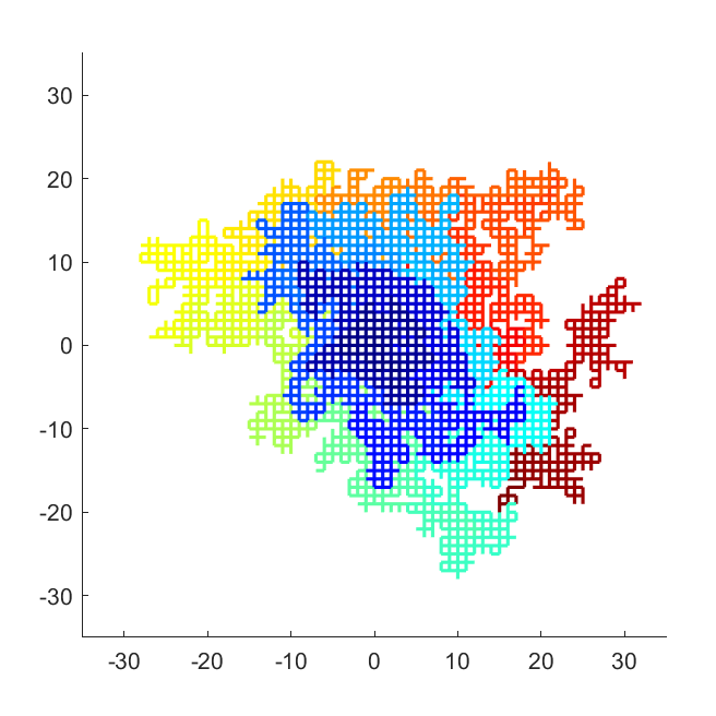
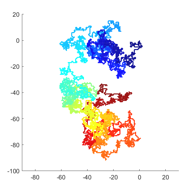
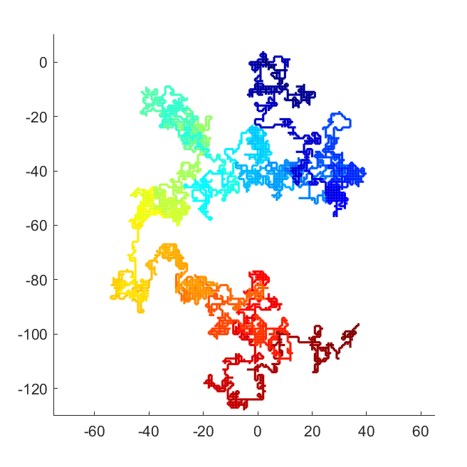
Figure 1. The vertices visited by the 10,000-step single walker version of the rotor walk (left), the $\operatorname{\mathcal{H}}$–$\operatorname{\mathcal{V}}$ walk with $q=1$ (middle), and the simple random walk (right) on $\mathbb{Z}^{2}$; these processes are ordered in increasing amount of randomness. Each edge is colored according to the time of its first visit by the walker.

The one-dimensional counterpart of $\operatorname{\mathcal{H}}$–$\operatorname{\mathcal{V}}$ walks, called $p$-rotor walks on $\operatorname{\mathbb{Z}}$, was studied in [HLSH18], where each vertex is labeled $L$ (left) or $R$ (right), and is changed to the opposite label with probability $p$ whenever the vertex is visited. The $p$-rotor walk is a special case of excited random walks with Markovian cookie stacks [KP17], where the labels evolve following the transition rules of a prescribed Markov chain. The recurrence and transience of these two models were studied in both works and are now completely understood. On the other hand, until recently, very little was known for the recurrence and transience in higher dimensions. From this perspective, this paper aims to begin extending their works to higher dimensions, for which some standard methods for $\operatorname{\mathbb{Z}}$ (e.g., generalized Ray-Knight theory [Tót96]) cannot be applied anymore.

In analyzing $\operatorname{\mathcal{H}}$–$\operatorname{\mathcal{V}}$ walks, we take our inspiration from the theory of random walks in random environment (see e.g., [Zei04, Szn04]), in which the environment (i.e., the labels at each vertex) affects the motion of the walker, but the walker does not affect the environment. In contrast, with $\operatorname{\mathcal{H}}$–$\operatorname{\mathcal{V}}$ walks, the environment evolves in tandem with the motion of the walkers. This necessitates a different approach for proving recurrence, as common approaches in random walks in random environments (e.g., Nash-Williams inequality, see [Zei04, Lemma A.2]) cannot be applied to nonstatic environments.

1.1. Main results

We now present the main results of this paper.

Theorem 1.1.

Let  $q>0$  and  $n\geq\lfloor\frac{|4q-2|}{q}\rfloor+1$ . Then, for every choice of the initial labels at each vertex, the $\operatorname{\mathcal{H}}$–$\operatorname{\mathcal{V}}$ walk with $n$ walkers is recurrent.

Described in words, excepting the case $q=0$ (i.e., when the environment is not altered by the walkers),  $\operatorname{\mathcal{H}}$–$\operatorname{\mathcal{V}}$ walks can always be made recurrent by adding a fixed number of walkers. In this respect Theorem 1.1 is the best outcome one could hope for as for $q=0$ one can choose the initial labels so that the $\operatorname{\mathcal{H}}$–$\operatorname{\mathcal{V}}$ walk is never recurrent regardless of the number of walkers (see Section 8.2).

As a consequence of Theorem 1.1, we have the following corollary for $\operatorname{\mathcal{H}}$–$\operatorname{\mathcal{V}}$ walks with a single walker.

Corollary 1.2.

Let $q\in(\frac{2}{5},\frac{2}{3})$. Then, for every choice of the initial labels at each vertex, the $\operatorname{\mathcal{H}}$–$\operatorname{\mathcal{V}}$ walk with a single walker is recurrent.

When the labels are sampled from the $\operatorname{\mathsf{IID}}$ uniform measure on $\{\operatorname{\mathcal{H}},\operatorname{\mathcal{V}}\}$, the recurrence regime in Corollary 1.2 can be expanded even further.

Theorem 1.3.

Let $q\in(\frac{1}{3},1]$, and let the initial labels be drawn independently and uniformly from  $\{\operatorname{\mathcal{H}},\operatorname{\mathcal{V}}\}$ . Then the $\operatorname{\mathcal{H}}$–$\operatorname{\mathcal{V}}$ walk with a single walker is recurrent a.s..

The case $q=1$ in Theorem 1.3 deserves a special mention, as this $\operatorname{\mathcal{H}}$–$\operatorname{\mathcal{V}}$ walk is non-elliptic, a property that also applies to rotor walks. (A walk is elliptic if, every neighbor of the current location of the walker, is visited at the next step with positive probability.) Most recurrence and transience results in this area (e.g., [KOS16, KP17, PT17]) assume some versions of ellipticity, and thus Theorem 1.3 holds the distinction of being one of the few results in this area for non-elliptic walks.

In the proof of Theorem 1.1 and Theorem 1.3, we use martingales that track both the number of departures from the origin and the labels at each vertex at any given time (see Definition 4.3), combined with zero-one laws that we develop for the recurrence of $\operatorname{\mathcal{H}}$–$\operatorname{\mathcal{V}}$ walks (see Section 2.3). By applying the optional stopping theorem to the martingales, we derive lower bounds for the return probabilities $p_{k}$ (i.e., the probability that the number of returns to the origin is at least $k$). These lower bounds turn out to be uniformly bounded away from $0$ under the hypotheses of Theorem 1.1, and we then use a zero-one law (see Proposition 2.9) to conclude that the walk is recurrent.

When the labels are sampled from the $\operatorname{\mathsf{IID}}$ uniform measure on $\{\operatorname{\mathcal{H}},\operatorname{\mathcal{V}}\}$, we derive improved lower bounds (see (24)), which are again uniformly bounded away from $0$ when $q$ is contained in the interval $(\frac{1}{3},1)$ (note that this regime does not include $q=1$). However, for the case $q=1$, these improved lower bounds yield only the trivial lower bound, and thus we need to improve them even further. We achieve this further improvement by proving an anti-concentration inequality, for the probability of the label of an arbitrary vertex being equal to a given label (see Lemma 7.3). Finally, we use another zero-one law (see Proposition 2.10) to conclude that the walk is recurrent.

1.2. Comparison with previous works

The martingale approach in this paper dates back to the work of Holroyd and Propp [HP10], and since then has been successfully applied to prove various results for rotor walks (see e.g., [HS11, FGLP14, Cha20]) and $p$-rotor walks (see e.g.,[HLSH18]). The zero-one laws for the recurrence of $\operatorname{\mathcal{H}}$–$\operatorname{\mathcal{V}}$ walks are inspired by zero-one laws for the directional transience of excited cookie random walks (see [KZ13] and references therein), but with proofs based on the work of [AH12] originally developed for rotor walks. The anti-concentration inequality, used in the proof of Theorem 1.3 for $q=1$, is original to this paper, to the best of the author’s knowledge.

1.3. Related works

$\operatorname{\mathcal{H}}$–$\operatorname{\mathcal{V}}$ walks are randomized versions of rotor walks (discovered independently by [PDDK96, WLB96, Pro03]), where the last exit from each vertex follows an assigned deterministic order. Ander and Holroyd [AH12] showed that, one can always find a labeling for vertices of $\operatorname{\mathbb{Z}}^{d}$ ($d\geq 1$) such that the (single walker) rotor walk is recurrent. On the other end of the spectrum, Florescu et al. [FGLP14] and Chan [Cha19] constructed different labelings for vertices of $\operatorname{\mathbb{Z}}^{d}$ ($d\geq 3$) for which the rotor walk is transient regardless of the number of walkers. The recurrence and transience of rotor walks have also been investigated for other graphs, including regular trees [LL09, AH11, MO17], Galton-Watson trees [HMSH15], directed cover of graphs [HS12], and oriented lattices [FLP16]. Notably, the recurrence of rotor walks on $\operatorname{\mathbb{Z}}^{2}$ with labels sampled from the $\operatorname{\mathsf{IID}}$ uniform measure on $\{\text{up, down, left, right}\}$ remains an open problem despite numerous investigations of this subject. We refer the reader to [HLM⁺08] for an excellent exposition on rotor walks and related subjects.

$\operatorname{\mathcal{H}}$–$\operatorname{\mathcal{V}}$ walks were introduced in [CGLL18] as the representative example of random walks with local memory, or RWLM for short, where each vertex stores one bit of information by remembering the last exit from the vertex, and the next exit is determined by the transition rule of a local Markov chain assigned to the vertex. We discuss RWLMs in more details in Section 2, where we derive zero-one laws for their recurrence.

One dimensional RWLMs are more commonly studied in the literature under the name excited random walks, or cookie random walks: A pile of cookies is initially placed at each vertex of $\operatorname{\mathbb{Z}}$. Upon visiting a vertex, the walker consumes the topmost cookie from the pile and moves one step to the right or to the left with probabilities prescribed by that cookie. If there are no cookies left at the current vertex, the walker moves one step to the right or to the left with equal probabilities. A cookie is positive (resp. negative) if its consumption makes the walker moves right with probability larger (resp. smaller) than $\frac{1}{2}$. The recurrence and transience of cookie random walks on $\operatorname{\mathbb{Z}}$ have been studied for the case of nonnegative cookies [Zer05], bounded number of cookies per site [KZ08], periodic cookies [KOS16], stationary-ergodic cookie distribution [ABO16], iterated leftover environments [AO16], site-based feedback environment [PT17], and Markovian cookie stacks [KP17] (the last two papers are the most relevant to this paper). Cookie random walks on $\operatorname{\mathbb{Z}}^{d}$ with $d>1$ are not studied as well as those on $\operatorname{\mathbb{Z}}$. Works which consider $d>1$ include the case of a single cookie per vertex [BW03], the case of walks with a positive drift on one direction [Zer06] (note that $\operatorname{\mathcal{H}}$–$\operatorname{\mathcal{V}}$ walks have no drift), and a generalized case called generalized excited random walks [MPRV12]. We refer the reader to [KZ13] for an excellent exposition on this subject.

Reinforced random walks (introduced by [CD87], see also [Pem88]) have the walkers choose their next location with probability dependent to the number of visits to that location so far. Thus the next exit from a vertex depends on all the past visits, instead of only the most recent visit. We refer the reader to [Tót01, Pem07] for slightly dated but very useful surveys on this subject. Important works on reinforced random walks published after those surveys include [ACK14, ST15, DST15, SZ19].

1.4. Outline

In Section 2, we introduce stack walks and random walks with local memory, and we present zero-one laws for the recurrence of these walks. In Section 3, we restate the main results in the notation of Section 2. In Section 4, we introduce the martingales and prove lower bounds for the return probabilities. In Section 5, we prove Theorem 1.1. In Section 6, we prove Theorem 1.3 for $q\in(\frac{1}{3},1)$. In Section 7, we prove Theorem 1.3 for $q=1$. In Section 8, we give concluding remarks and discuss open questions.

2. Preliminaries

In this paper $G:=(V,E)$ is a (possibly infinite) graph that is simple, connected, and locally finite (every vertex has finite degree). A neighbor of a vertex $x\in V$ is another vertex $y\in V$ such that $\{x,y\}$ is an edge of $G$. We denote by $\operatorname{{Ngh}}(x)$ the set of neighbors of $x$. We denote by $\operatorname{\mathbb{N}}$ the set of all nonnegative integers $\{0,1,2,\ldots\}$.

2.1. Stack walks

A stack of $G$ is a function $\xi:V\times\operatorname{\mathbb{N}}\to V$ such that, for all $x\in V$ and $m\geq 0$, we have $\xi(x,m)$ is a neighbor of $x$.

Definition 2.1 (Stack walks).

Let $x$ be a vertex of $G$, and let $\xi$ be a stack of $G$. A stack walk with initialization $(x,\xi)$ is the sequence $(X_{t},\xi_{t})_{t\geq 0}$ defined recursively by

(1) $$\begin{split}(X_{0},\xi_{0})&\ :=\ (x,\xi);\\ \xi_{t+1}(x,\cdot)&\ :=\ \begin{cases}\xi_{t}(x,\cdot+1)&\text{if $x=X_{t}$};\\ \xi_{t}(x,\cdot)&\text{if $x\neq X_{t}$};\end{cases}\\ X_{t+1}&\ :=\ \xi_{t+1}(X_{t},0).\end{split}$$

Note that the stack walk is determined by the initialization $(x,\xi)$.

The following image is useful: $X_{t}$ records the location of the walker at the end of the $t$-th step of the walk. For each $x\in V$, we think of $\xi_{t}(x,\cdot)$ as a stack lying under the vertex $x$ with $\xi_{t}(x,0)$ being on top, then $\xi_{t}(x,1)$, and so forth. Then, at the $t+1$-th step, the walker pops off the stack of its current location $X_{t}$, meaning that it removes the top item of the stack lying under $X_{t}$. Then, the walker moves to the vertex specified by the top item of the new stack. This description of the walk originated from the work of Diaconis and Fulton [DF91], and the term stack walk was coined by Holroyd and Propp [HP10]. The stack walk was featured prominently in Wilson’s algorithm for the uniform sampling of spanning trees of a finite graph [Wil96].

We will also consider the multi-walker version of stack walks in this paper.

Definition 2.2 (Multi-walker stack walks).

Let $n\geq 1$ be the number of walkers, let $\operatorname{\mathbf{x}}=(x^{(1)},\ldots,x^{(n)})\in V^{n}$ be the initial location of the $n$ walkers, and let $\xi$ be the initial stack. A turn order is a sequence  $\operatorname{\mathcal{O}}=o_{1}o_{2}\ldots$  such that each $o_{t}$ is contained in  $\{0,\ldots,n\}$ The multi-walker stack walk  $(\operatorname{\mathbf{X}}_{t}=(X_{t}^{(1)},\ldots,X_{t}^{(n)}),\xi_{t})_{t\geq 0}$  is defined recursively as follows:

$$\begin{split}(\operatorname{\mathbf{X}}_{0},\xi_{0})&\ :=\ (\operatorname{\mathbf{x}},\xi);\\ \xi_{t+1}(x,\cdot)&\ :=\ \begin{cases}\xi_{t}(x,\cdot+1)&\text{if \ $x=X_{t}^{(i)}$ \ and \ $i=o_{t+1}$};\\ \xi_{t}(x,\cdot)&\text{otherwise};\end{cases}\\ X_{t+1}^{(i)}&\ :=\ \begin{cases}\xi_{t+1}(X_{t}^{(i)},0)&\text{if \ $i=o_{t+1}$};\\ X_{t}^{(i)}&\text{otherwise.}\end{cases}\end{split}$$

Note that, once the turn order $\mathcal{O}$ is fixed, the multi-walker stack walk is determined by the initialization $(\operatorname{\mathbf{x}},\xi)$.

Described in words, at the $t$-th step of the walk, the $o_{t}$-th walker performs one step of the stack walk, with $\operatorname{\mathbf{X}}_{t}$ and $\xi_{t}$ tracking the location of the $n$ walkers and the stack after the first $t$ steps of the walk. Note that the $n$ walkers are sharing the same stack when performing the stack walk. Also note that $o_{t}=0$ means that none of the walkers move (for example, this can occur when some stopping condition has been reached, see §4.1).

A multi-walker stack walk is recurrent if every vertex is visited infinitely many times, and is transient if every vertex is visited at most finitely many times. A stack $\xi$ of $G$ is regular if, for every $x\in V$, every neighbor $y$ of $x$ appears in the stack $\xi(x,\cdot)$ infinitely many times. A turn order is regular if every walker performs infinitely many steps, i.e., each $i\in\{1,\ldots,n\}$ appears in $\operatorname{\mathcal{O}}$ infinitely many times.

Lemma 2.3 ([HP10, Lemma 6]).

Let  $(\operatorname{\mathbf{X}}_{t},\xi_{t})_{t\geq 0}$  be a multi-walker stack walk with a regular turn order and a regular initial stack. Then the walk is either recurrent or transient. ∎

Proof.

Suppose that the stack walk is not transient. Then there exists $x\in V$ that is visited infinitely many times. It thus suffices to show that

(2) If a vertex $$x\in V$$ is visited infinitely many times, then the stack walk is recurrent.

Since the initial stack and the turn order are both regular, this implies that every neighbor of $x$ is also visited infinitely many times. Since $G$ is connected, repeating the same argument ad infinitum implies that every vertex of $G$ is visited infinitely many times. This implies that the stack walk is recurrent if it is not transient, as desired. ∎

For every $x\in V$ and $t\geq 0$, we denote by  $R_{t}(x):=R_{t}(x;\operatorname{\mathbf{X}},\xi,\operatorname{\mathcal{O}})$  the total number of transitions (also the number of visits) to $x$ by the stack walk up to time $t$,

$$R_{t}(x)\ :=\ \big{|}\{s\in\{1,\ldots,t\}\hskip 1.70709pt\mid\hskip 1.70709ptX_{s-1}^{(i)}\neq x,\ X_{s}^{(i)}=x\ \text{ for some }i\in\{1,\ldots,n\}\}\big{|}\hskip 1.70709pt.$$

We write  $R_{\infty}(x):=\lim_{t\to\infty}R_{t}(x)$  the total number of transitions to $x$ throughout the entirety of the stack walk.

Lemma 2.4.

Let $\operatorname{\mathcal{O}}$ and $\operatorname{\mathcal{O}}^{\prime}$ be turn orders for two stack walks with the same initial location and the same initial stack. Suppose that $\operatorname{\mathcal{O}}^{\prime}$ is a regular turn order. Then, for every $x\in V$,

$$R_{\infty}(x)\quad\leq\quad R_{\infty}^{\prime}(x),$$

the total number of visits to $x$ by the stack walk with turn order $\operatorname{\mathcal{O}}$ is less than or equal to that of the stack walk with turn order $\operatorname{\mathcal{O}}^{\prime}$.

We present the proof of Lemma 2.4 in Appendix A, and the proof is adapted from [BL16, Lemma 4.3] for abelian networks (see also [CL18, Corollary 4.3] for an alternate proof).

Lemma 2.5 (Abelian property).

Let $\operatorname{\mathcal{O}}$ and $\operatorname{\mathcal{O}}^{\prime}$ be regular turn orders for two stack walks with the same initial location and the same initial stack. Then the stack walk with turn order $\operatorname{\mathcal{O}}$ is recurrent if and only if the stack walk with turn order $\operatorname{\mathcal{O}}^{\prime}$ is recurrent.

Proof.

This follows directly from Lemma 2.4. ∎

Thus we omit the dependence on the turn order from the notation, and we assume throughout this paper the cyclic turn order (i.e., $o_{t}$ is the unique integer in $\{1,\ldots,n\}$ that is equal to $t$ modulo $n$)  is used, unless stated otherwise. Note that the cyclic turn order is regular.

For every $\operatorname{\mathbf{x}}\in V^{n}$ and every stack $\xi$, we say $(\operatorname{\mathbf{x}},\xi)$ is recurrent if the stack walk with initialization $(\operatorname{\mathbf{x}},\xi)$ is recurrent. Similarly, we say $(\operatorname{\mathbf{x}},\xi)$ is transient if the stack walk with initialization $(\operatorname{\mathbf{x}},\xi)$ is transient. We also write

$$\operatorname{\mathbbm{1}}_{\operatorname{\textnormal{rec}}}(\operatorname{\mathbf{x}},\xi)\ :=\ \begin{cases}1&\text{ if }(\operatorname{\mathbf{x}},\xi)\text{ is recurrent};\\ 0&\text{ if }(\operatorname{\mathbf{x}},\xi)\text{ is transient}.\end{cases}$$

For every $x\in V$, the popping operation $\varphi_{x}$ is a map that sends a stack $\xi$ to the stack $\varphi_{x}(\xi)$ by popping off the top item of the stack of $x$,

$$\varphi_{x}(\xi)(y,m)\ :=\ \begin{cases}\xi(y,m+1)&\text{ if }y=x;\\ \xi(y,m)&\text{ if }y\neq x.\end{cases}$$

We say that a stack $\xi^{\prime}$ is obtained from $\xi$ by finitely many popping operations if there exists $x_{1},\ldots,x_{m}\in V$ such that  $\varphi_{x_{m}}\circ\cdots\circ\varphi_{x_{1}}(\xi)\hskip 1.70709pt=\hskip 1.70709pt\xi^{\prime}$ . In particular, for every stack walk  $(\operatorname{\mathbf{X}}_{t},\xi_{t})_{t\geq 0}$  and every $t\geq 0$, the stack $\xi_{t}$ is obtained from $\xi_{0}$ by finitely many popping operations.

Theorem 2.6 (c.f. [AH12, Theorem 1, Corollary 6]).

Let $\operatorname{\mathbf{x}},\operatorname{\mathbf{x}}^{\prime}\in V^{n}$ and let $\xi,\xi^{\prime}$ be regular stacks such that $\xi^{\prime}$ is obtained from $\xi$ by finitely many popping operations. Then $(\operatorname{\mathbf{x}},\xi)$ is recurrent if and only if $(\operatorname{\mathbf{x}}^{\prime},\xi^{\prime})$ is recurrent. ∎

We present the proof of Theorem 2.6 in Appendix B for completeness, and the proof is adapted from [AH12].

2.2. Random walks with local memory

A random walk with local memory is the following randomized version of stack walks. A rotor configuration is a function $\rho:V\to V$ such that $\rho(x)$ is a neighbor of $x$ for all $x\in V$. We assign a local mechanism $\operatorname{\mathcal{M}}_{x}$ for each $x\in V$, which is a Markov chain with states $\operatorname{{Ngh}}(x)$ and with transition function  $p_{x}(\cdot,\cdot)$ . We assume that $\operatorname{\mathcal{M}}_{x}$ is an irreducible Markov chain. Note that each $\operatorname{\mathcal{M}}_{x}$ is a Markov chain with a finite state space since the graph is locally finite.

Definition 2.7 (Random walk with local memory).

Let $n\geq 1$, let $\operatorname{\mathbf{x}}\in V^{n}$, and let $\rho$ be a rotor configuration. A (multi-walker) random walk with local memory with initialization $(\operatorname{\mathbf{x}},\rho)$, or RWLM for short, is a random sequence of pairs $(\operatorname{\mathbf{X}}_{t},\rho_{t})_{t\geq 0}$ that satisfies the following transition rule:

(3) $$\begin{split}(\operatorname{\mathbf{X}}_{0},\rho_{0})\ :=\ &(\operatorname{\mathbf{x}},\rho);\\ \rho_{t+1}(x)\ :=\ &\begin{cases}Y_{t}&\text{if \ $x=X_{t}^{(i)}$ \ and \ $i\equiv t+1$ mod $n$};\\ \rho_{t}(x)&\text{otherwise,}\end{cases};\text{ and }\\ X_{t+1}^{(i)}\ :=\ &\begin{cases}Y_{t}&\text{if \ $i\equiv t+1$ mod $n$};\\ X_{t}^{(i)}&\text{otherwise,}\end{cases}\end{split}$$

where $Y_{t}$ is a random neighbor of $X_{t}^{(i)}$ sampled from  $p_{X_{t}^{(i)}}(\rho_{t}(X_{t}^{(i)}),\cdot)$  with $i$ satisfying $i\equiv t+1$ mod $n$, independent of the past.

We refer to [CGLL18] for history and references for random walks with local memory.

The following image is useful: The random walk with local memory  $(\operatorname{\mathbf{X}}_{t},\rho_{t})_{n\geq 0}$  corresponds to the (random) stack walk  $(\operatorname{\mathbf{X}}_{t},\xi_{t})_{t\geq 0}$ , where, for each $x\in V$, the initial stack  $\xi_{0}(x,\cdot)$  is a Markov process for the Markov chain $\operatorname{\mathcal{M}}_{x}$ with initial state $\rho(x)$. We denote by $\operatorname{\mathsf{Stack}}(\rho)$ the corresponding probability distribution on stacks of $G$, which is the source of the randomness in the RWLM. Note that, for each $t\geq 0$, the vector $\operatorname{\mathbf{X}}_{t}$ records the location of the walkers for both walks (the RWLM and the (random) stack walk) and the rotor $\rho_{t}(x)$ at $x$ corresponds to the top item $\xi_{t}(x,0)$ of the stack $\xi_{t}$.

Let $\rho$ be an arbitrary rotor configuration of $G$. The recurrence probability  $p_{\operatorname{\textnormal{rec}}}(\rho)$  is the probability that the RWLM with initial rotor configuration $\rho$ is recurrent,

$$p_{\operatorname{\textnormal{rec}}}(\rho)\ :=\ \operatorname{\mathbb{E}}_{\xi\sim\operatorname{\mathsf{Stack}}(\rho)}\hskip 1.70709pt\big{[}\operatorname{\mathbbm{1}}_{\operatorname{\textnormal{rec}}}(\operatorname{\mathbf{x}},\xi)\big{]}\hskip 1.70709pt,$$

where $\operatorname{\mathbf{x}}$ is an arbitrary element of $V^{n}$. Note that  $p_{\operatorname{\textnormal{rec}}}(\rho)$  does not depend on the choice of $\operatorname{\mathbf{x}}\in V^{n}$ by Theorem 2.6. However,  $p_{\operatorname{\textnormal{rec}}}(\rho)$  could depend on the number of walkers $n$ (the dependence on $n$ is not reflected in the notation for simplicity).

We say that two rotor configuration $\rho,\rho^{\prime}$ differ by finitely many vertices if there exists $x_{1},\ldots,x_{m}$ such that  $\rho(x)=\rho^{\prime}(x)$  for all $x\in V\setminus\{x_{1},\ldots,x_{m}\}$ .

Lemma 2.8.

Let $\rho$ and $\rho^{\prime}$ be rotor configurations that differ by finitely many vertices. Then

$$p_{\operatorname{\textnormal{rec}}}(\rho)\ =\ p_{\operatorname{\textnormal{rec}}}(\rho^{\prime})\hskip 1.70709pt.$$

Proof.

Let $\xi$ be the stack sampled from $\operatorname{\mathsf{Stack}}(\rho)$. Note that $\xi$ is a regular stack a.s. since every local mechanism $\operatorname{\mathcal{M}}_{x}$ is an irreducible Markov chain with a finite state space. For each $y\in V$, let $T_{y}$ be the (random) smallest nonnegative integer such that  $\xi(y,T_{y})\ =\ \rho^{\prime}(y)$ . We write  $\varphi:=\prod_{y\in V}\varphi_{y}^{T(y)}$ . Then, by the Markov property,

(4) $$\varphi\big{(}\xi\big{)}\ \text{ is equal in distribution to the stack sampled from }\hskip 1.70709pt\operatorname{\mathsf{Stack}}(\rho^{\prime})\hskip 1.70709pt.$$

Note that $T_{y}=0$ for all but finitely many $y$’s since $\rho$ and $\rho^{\prime}$ differ by finitely many vertices. Also note that each $T_{y}$ is finite a.s. since the Markov chain $\operatorname{\mathcal{M}}_{y}$ is irreducible and finite. These two observations imply that $\varphi$ is a finite product of popping operations a.s.. It then follows from Theorem 2.6 that, for all $\operatorname{\mathbf{x}}\in V^{n}$,

(5) $$\operatorname{\mathbbm{1}}_{\operatorname{\textnormal{rec}}}\big{(}\operatorname{\mathbf{x}},\varphi\big{(}\xi\big{)}\big{)}\ =\ \operatorname{\mathbbm{1}}_{\operatorname{\textnormal{rec}}}\big{(}\operatorname{\mathbf{x}},\xi\big{)}\quad\text{a.s.}$$

Combining (4) and (5), we get

$$p_{\operatorname{\textnormal{rec}}}(\rho)\quad =\quad\operatorname{\mathbb{E}}_{\xi\sim\operatorname{\mathsf{Stack}}(\rho)}\hskip 1.70709pt\big{[}\operatorname{\mathbbm{1}}_{\operatorname{\textnormal{rec}}}(\operatorname{\mathbf{x}},\xi)\big{]}\quad=_{\eqref{equation: alfa 2}}\quad\operatorname{\mathbb{E}}_{\xi\sim\operatorname{\mathsf{Stack}}(\rho)}\hskip 1.70709pt\big{[}\operatorname{\mathbbm{1}}_{\operatorname{\textnormal{rec}}}\big{(}\operatorname{\mathbf{x}},\varphi(\xi)\big{)}\big{]}$$

$$=_{\eqref{equation: alfa 1}}\quad\operatorname{\mathbb{E}}_{\xi^{\prime}\sim\operatorname{\mathsf{Stack}}(\rho^{\prime})}\hskip 1.70709pt\big{[}\operatorname{\mathbbm{1}}_{\operatorname{\textnormal{rec}}}(\operatorname{\mathbf{x}},\xi^{\prime})\big{]}\quad=\quad p_{\operatorname{\textnormal{rec}}}(\rho^{\prime})\hskip 1.70709pt,$$

as desired. ∎

2.3. Zero-one laws for recurrence

In this subsection we prove several zero-one laws for the recurrence of RWLMs. (These zero-one laws are not to be confused with zero-one laws for the directional transience of cookie random walks (see e.g., [KZ13])).

Proposition 2.9.

Consider an RWLM with the initial rotor configuration $\rho$. Then the recurrence probability satisfies

$$p_{\operatorname{\textnormal{rec}}}(\rho)\ \in\ \{0,1\}\hskip 1.70709pt.$$

We then say that a rotor configuration $\rho$ is recurrent (with respect to the RWLM) if $p_{\operatorname{\textnormal{rec}}}(\rho)=1$, and is transient if $p_{\operatorname{\textnormal{rec}}}(\rho)=0$.

We now present the proof of Proposition 2.9.

Proof of Proposition 2.9.

Let $\operatorname{\mathbf{x}}$ be an arbitrary element of $V^{n}$, let $(\operatorname{\mathbf{X}}_{t},\rho_{t})_{t\geq 0}$ be the RWLM with initialization $(\operatorname{\mathbf{x}},\rho)$, and let $(\operatorname{\mathbf{X}}_{t},\xi_{t})_{t\geq 0}$ be the corresponding stack walk. We write  $\operatorname{\mathcal{F}}_{m}:=\sigma(\operatorname{\mathbf{X}}_{0},\rho_{0},\ldots\operatorname{\mathbf{X}}_{m},\rho_{m})$  ($m\geq 0$) . Note that $(\operatorname{\mathcal{F}}_{m})_{m\geq 0}$ is a filtration by definition.

Let $m\geq 0$. Note that the stack walk  $(\operatorname{\mathbf{X}}_{t},\xi_{t})_{t\geq 0}$  is recurrent   if and only if   the stack walk  $(\operatorname{\mathbf{X}}_{t+m},\xi_{t+m})_{t\geq 0}$  is recurrent. This implies that, the pair  $(\operatorname{\mathbf{x}},\xi)$  is recurrent, if and only if, the pair  $(\operatorname{\mathbf{X}}_{m},\xi_{m})$  is recurrent. It then follows that

$$\operatorname{\mathbb{E}}_{\xi\sim\operatorname{\mathsf{Stack}}(\rho)}\big{[}\operatorname{\mathbbm{1}}_{\operatorname{\textnormal{rec}}}\big{(}\operatorname{\mathbf{x}},\xi\big{)}\hskip 1.70709pt\big{|}\hskip 1.70709pt\operatorname{\mathcal{F}}_{m}\big{]}\quad =\quad\operatorname{\mathbb{E}}_{\xi\sim\operatorname{\mathsf{Stack}}(\rho)}\big{[}\operatorname{\mathbbm{1}}_{\operatorname{\textnormal{rec}}}\big{(}\operatorname{\mathbf{X}}_{m},\xi_{m}\big{)}\hskip 1.70709pt\big{|}\hskip 1.70709pt\operatorname{\mathcal{F}}_{m}\big{]}$$

$$=_{\text{Thm}~{}\ref{theorem: recurrence is invariant under stack relation}}\quad\operatorname{\mathbb{E}}_{\xi\sim\operatorname{\mathsf{Stack}}(\rho)}\big{[}\operatorname{\mathbbm{1}}_{\operatorname{\textnormal{rec}}}\big{(}\operatorname{\mathbf{x}},\xi_{m}\big{)}\hskip 1.70709pt\big{|}\hskip 1.70709pt\operatorname{\mathcal{F}}_{m}\big{]}\hskip 1.70709pt.$$

Now note that $\xi_{m}$ is equal in distribution to $\operatorname{\mathsf{Stack}}(\rho_{m})$, and $\rho_{m}$ is adapted to $\operatorname{\mathcal{F}}_{m}$. Plugging these observations into the equation above,

(6) $$\operatorname{\mathbb{E}}_{\xi\sim\operatorname{\mathsf{Stack}}(\rho)}\big{[}\operatorname{\mathbbm{1}}_{\operatorname{\textnormal{rec}}}\big{(}\operatorname{\mathbf{x}},\xi\big{)}\hskip 1.70709pt\big{|}\hskip 1.70709pt\operatorname{\mathcal{F}}_{m}\big{]}\quad= \quad\operatorname{\mathbb{E}}_{\xi^{\prime}\sim\operatorname{\mathsf{Stack}}(\rho_{m})}\big{[}\operatorname{\mathbbm{1}}_{\operatorname{\textnormal{rec}}}\big{(}\operatorname{\mathbf{x}},\xi^{\prime}\big{)}\big{]}\quad=\quad p_{\operatorname{\textnormal{rec}}}(\rho_{m})\hskip 1.70709pt.$$

(Note that $p_{\operatorname{\textnormal{rec}}}(\rho_{m})$ here is regarded as a random variable adapted to $\operatorname{\mathcal{F}}_{m}$.) On the other hand, since $\rho_{m}$ differs from $\rho$ by at most $m$ many vertices, it follows from Lemma 2.8 that   $p_{\operatorname{\textnormal{rec}}}(\rho_{m})\hskip 1.70709pt=\hskip 1.70709ptp_{\operatorname{\textnormal{rec}}}(\rho)$ . Combining this observation with (6) gives us

(7) $$\operatorname{\mathbb{E}}_{\xi\sim\operatorname{\mathsf{Stack}}(\rho)}\big{[}\operatorname{\mathbbm{1}}_{\operatorname{\textnormal{rec}}}\big{(}\operatorname{\mathbf{x}},\xi\big{)}\hskip 1.70709pt\big{|}\hskip 1.70709pt\operatorname{\mathcal{F}}_{m}\big{]}\quad= \quad p_{\operatorname{\textnormal{rec}}}(\rho).$$

Thus we have

(8) $$p_{\operatorname{\textnormal{rec}}}(\rho)\quad=\quad\operatorname{\mathbb{E}}_{\xi\sim\operatorname{\mathsf{Stack}}(\rho)}\big{[}\operatorname{\mathbbm{1}}_{\operatorname{\textnormal{rec}}}\big{(}\operatorname{\mathbf{x}},\xi\big{)}\hskip 1.70709pt\big{|}\hskip 1.70709pt\operatorname{\mathcal{F}}_{m}\big{]}\quad\overset{m\to\infty}{\longrightarrow}\quad\operatorname{\mathbbm{1}}_{\operatorname{\textnormal{rec}}}\big{(}\operatorname{\mathbf{x}},\xi\big{)}\qquad\operatorname{\mathcal{F}}_{\infty}\text{-a.s.},$$

where the convergence in the equation above is due to Levy’s zero-one law (see e.g. [Dur19, Theorem 4.6.9]). Since $p_{\operatorname{\textnormal{rec}}}(\rho)$ is a constant that does not depend on $m$, it then follows from (8) that $p_{\operatorname{\textnormal{rec}}}(\rho)\in\{0,1\}$, as desired. ∎

Let  $\operatorname{\mathsf{IUD}}$  be the probability measure on rotor configurations of $G$ where the rotor for $x\in V$ is chosen independently and uniformly at random from the neighbors of $x$. (By an abuse of the notation, we refer to this measure as the $\operatorname{\mathsf{IUD}}$ measure, even though two different vertices can have different sets of neighbors, and thus different rotor distributions.) We now consider RWLMs in which the initial rotor configuration is sampled from  $\operatorname{\mathsf{IUD}}$ . Note that there are two (independent) layers of randomness involved in this process now: The first layer being the random initial rotor configuration, and the second layer being the transition rules of RWLM in (3).

Proposition 2.10.

Consider an RWLM with the initial rotor configuration $\rho$ sampled from the $\operatorname{\mathsf{IUD}}$ measure. Then exactly one of the following scenarios holds:

• $p_{\operatorname{\textnormal{rec}}}(\rho)\ =\ 0$   for almost every $\rho$ sampled from $\operatorname{\mathsf{IUD}}$; or

• $p_{\operatorname{\textnormal{rec}}}(\rho)\ =\ 1$  for almost every $\rho$ sampled from $\operatorname{\mathsf{IUD}}$.

Proof.

Let $x_{1},x_{2},\ldots$ be an arbitrary ordering of elements of $V$. Let  $\operatorname{\mathcal{F}}^{\prime}_{m}:=\sigma(\rho(x_{m}),\rho(x_{m+1}),\ldots)$  be the $\sigma$-field on rotor configurations of $G$ that depends only on the rotor configuration $\rho$ at $V\setminus\{x_{1},\ldots,x_{m-1}\}$. Let $A$ be the set of rotor configurations of $G$ given by

$$A\ :=\ \{\rho\mid p_{\operatorname{\textnormal{rec}}}(\rho)=1\}.$$

By Theorem 2.6, for arbitrary rotor configurations $\rho,\rho^{\prime}$ that differ by finitely many vertices, $\rho$ is contained in $A$ implies $\rho^{\prime}$ is also contained in $A$. This implies that $A\in\operatorname{\mathcal{F}}^{\prime}_{m}$ for every $m\geq 0$, and hence $A$ is contained in the tail $\sigma$-field  $\bigcap_{m\geq 0}\operatorname{\mathcal{F}}^{\prime}_{m}$. Since $\rho$ is sampled from the $\operatorname{\mathsf{IUD}}$ measure, it then follows from Kolmogorov’s zero-one law (see e.g., [Dur19, Thm 2.5.3]) that

$$\operatorname{\mathbb{P}}_{\rho\sim\operatorname{\mathsf{IUD}}}[A]\ \in\ \{0,1\}.$$

On the other hand, Proposition 2.9 gives us

$$\operatorname{\mathbb{P}}_{\rho\sim\operatorname{\mathsf{IUD}}}[A]\ =\ 0\qquad\text{implies}\qquad\text{$p_{\operatorname{\textnormal{rec}}}(\rho)\ =\ 0$ \ for almost every $\rho$ sampled from $\operatorname{\mathsf{IUD}}$;}$$

$$\operatorname{\mathbb{P}}_{\rho\sim\operatorname{\mathsf{IUD}}}[A]\ =\ 1\qquad\text{implies}\qquad\text{$p_{\operatorname{\textnormal{rec}}}(\rho)\ =\ 1$ \ for almost every $\rho$ sampled from $\operatorname{\mathsf{IUD}}$\hskip 1.70709pt.}$$

The proposition now follows from combining the two observations above. ∎

3. Horizontal-vertical walks

The horizontal-vertical walk, or $\operatorname{\mathcal{H}}$–$\operatorname{\mathcal{V}}$ walk for short, (introduced by Chan et al. [CGLL18]), is a nearest-neighbor random walk on $\operatorname{\mathbb{Z}}^{2}$, where each vertex of $\operatorname{\mathbb{Z}}^{2}$ is labeled either $\operatorname{\mathcal{H}}$ or $\operatorname{\mathcal{V}}$. Initially we have $n$ walkers dropped to the origin $(0,0)$ in $\operatorname{\mathbb{Z}}^{2}$. Each of the $n$ walkers performs the following move in a cyclic order: the chosen walker changes the label of its current location with probability $q\in[0,1]$, and does not change the label with probability $1-q$. Then, the walker takes a mean zero horizontal step if the new label is $\operatorname{\mathcal{H}}$, and a mean zero vertical step if the new label is $\operatorname{\mathcal{V}}$.

Formally, the $\operatorname{\mathcal{H}}$–$\operatorname{\mathcal{V}}$ walk is an instance of RWLM (see (3)) where each local mechanism $\operatorname{\mathcal{M}}_{x}$ is given by the transition rule

• If  $y_{1}-x\in\{(1,0),-(1,0)\}$ , then:

  $$p_{x}(y_{1},y_{2})\ =\ \begin{cases}\frac{1-q}{2}&\text{ if }\ y_{2}-x\in\{(1,0),-(1,0)\};\\ \frac{q}{2}&\text{ if }\ y_{2}-x\in\{(0,1),-(0,1)\}.\end{cases}$$

• If  $y_{1}-x\in\{(0,1),-(0,1)\}$ , then:

  $$p_{x}(y_{1},y_{2})\ =\ \begin{cases}\frac{q}{2}&\text{ if }\ y_{2}-x\in\{(1,0),-(1,0)\};\\ \frac{1-q}{2}&\text{ if }\ y_{2}-x\in\{(0,1),-(0,1)\}.\end{cases}$$

Note that this transition rule is equal to the one described in the beginning of the section. Indeed, the correspondence is

• A vertex $x$ is labeled $\operatorname{\mathcal{H}}$ if  $\rho(x)-x\in\{(1,0),-(1,0)\}$ ; and

• A vertex $x$ is labeled $\operatorname{\mathcal{V}}$ if  $\rho(x)-x\in\{(0,1),-(0,1)\}$ .

We will adopt the following notation throughout the rest of this paper:

• A rotor configuration $\rho$ is simultaneously, a function $\rho:V\to V$, and a function $\rho:V\to\{\operatorname{\mathcal{H}},\operatorname{\mathcal{V}}\}$, by the correspondence above;

• $q$ is strictly greater than $0$. This is so that, for each $x\in V$, the local mechanism $\operatorname{\mathcal{M}}_{x}$ for the $\operatorname{\mathcal{H}}$–$\operatorname{\mathcal{V}}$ walk is irreducible.

• $\operatorname{\mathbb{P}}$  and  $\operatorname{\mathbb{E}}$  will be shorthands for $\operatorname{\mathbb{P}}_{\xi\sim\operatorname{\mathsf{Stack}}(\rho)}$ and  $\operatorname{\mathbb{E}}_{\xi\sim\operatorname{\mathsf{Stack}}(\rho)}$ , respectively. Recall from Section 2.2 that $\xi$ is the random stack on $\operatorname{\mathbb{Z}}^{2}$ that arises from the Markov chains corresponding to the local mechanisms of the $\operatorname{\mathcal{H}}$–$\operatorname{\mathcal{V}}$ walk with initialization $\rho$. (Note that the random stack $\xi$ is the source of randomness for the $\operatorname{\mathcal{H}}$–$\operatorname{\mathcal{V}}$ walk.)

We now restate the main results in Section 1 using the notation in Section 2.

Theorem 1.1.

Let  $q>0$  and  $n\geq\lfloor\frac{|4q-2|}{q}\rfloor+1$ . Then, for every initial rotor configuration $\rho$, the corresponding $\operatorname{\mathcal{H}}$–$\operatorname{\mathcal{V}}$ walk with $n$ walkers satisfies

$$p_{\operatorname{\textnormal{rec}}}(\rho)=1.$$

We will prove Theorem 1.1 in Section 5. The following is a corollary of Theorem 1.1 for walks with a single walker.

Corollary 1.2.

Let $q\in(\frac{2}{5},\frac{2}{3})$ and $n=1$. Then, for every initial rotor configuration $\rho$, the corresponding $\operatorname{\mathcal{H}}$–$\operatorname{\mathcal{V}}$ walk with a single walker satisfies

$$p_{\operatorname{\textnormal{rec}}}(\rho)=1.\qed$$

When $\rho$ is sampled from $\operatorname{\mathsf{IUD}}$ measure, the recurrence regime in Corollary 1.2 can be expanded.

Theorem 1.3.

Let $q\in(\frac{1}{3},1]$, and let $n=1$. Then, for the $\operatorname{\mathcal{H}}$–$\operatorname{\mathcal{V}}$ walk with a single walker,

$$p_{\operatorname{\textnormal{rec}}}(\rho)\ =\ 1 \rho \operatorname{\mathsf{IUD}}$$   for  almost every rotor configuration   sampled from  .

We split the proof of Theorem 1.3 into two parts: we prove the case  $q\in(\frac{1}{3},1)$  in Section 6, and the case  $q=1$  in Section 7.

4. Martingale method

In this section we construct a martingale that tracks the number of departures from the origin by $\operatorname{\mathcal{H}}$–$\operatorname{\mathcal{V}}$ walks, and then we apply the optional stopping theorem to get a lower bound for the return probabilities of $\operatorname{\mathcal{H}}$–$\operatorname{\mathcal{V}}$ walks.

4.1. Frozen $\operatorname{\mathcal{H}}$–$\operatorname{\mathcal{V}}$ walks

Let $r\geq 1$. We denote by  $B_{r}$  the set of vertices in $\operatorname{\mathbb{Z}}^{2}$ that are of Euclidean distance strictly less than $r$ from the origin, and by $\partial B_{r}$ the outer boundary of $B_{r}$,

$$B_{r}\ :=\ \{x\in\operatorname{\mathbb{Z}}^{2}\hskip 1.70709pt\mid\hskip 1.70709pt|x|<r\};\qquad\partial B_{r}\ :=\ \{x\in\operatorname{\mathbb{Z}}^{2}\setminus B_{r}\hskip 1.70709pt\mid\hskip 1.70709ptN(x)\cap B_{r}\hskip 1.70709pt\neq\hskip 1.70709pt\varnothing\}\hskip 1.70709pt.$$

We now consider the variant of $\operatorname{\mathcal{H}}$–$\operatorname{\mathcal{V}}$ walks where each walker is immediately frozen if it reaches $\partial B_{r}$.

Definition 4.1 (Frozen $\operatorname{\mathcal{H}}$–$\operatorname{\mathcal{V}}$ walks).

Let $r\geq 1$, and let $\rho$ be a rotor configuration. The frozen $\operatorname{\mathcal{H}}$–$\operatorname{\mathcal{V}}$ walk  $(\operatorname{\mathbf{Y}}_{t}:=(Y_{t}^{(1)},\ldots,Y_{t}^{(n)}),\zeta_{t})_{t\geq 0}$  is defined recursively by

1. Initially $(\operatorname{\mathbf{Y}}_{0},\zeta_{0})\ :=\ \big{(}\big{(}(0,0),\ldots,(0,0)\big{)},\rho\big{)}$.

2. At the $t$-th step of the walk, let $i_{t}$ be the unique integer in $\{1,\ldots,n\}$ such that $i_{t}\equiv t\text{ mod }n$.

3. Let the $i_{t}$-th walker perform one step of the $\operatorname{\mathcal{H}}$–$\operatorname{\mathcal{V}}$ walk if its current location  $Y_{t}^{(i_{t})}$  is not contained in $\partial B_{r}$, and let the walker skip its turn if its current location is contained in $\partial B_{r}$ .

Note that both $\operatorname{\mathbf{Y}}_{t}$ and $\zeta_{t}$ are random variables that depend on $r$, and we do not write out their dependence on $r$ to lighten the notation.

We denote by  $R_{t,r}$  ($t\geq 0$)  the number of returns to the origin up to $t$ by the frozen walk,

$$R_{t,r}\quad:=\quad\big{|}\big{\{}s\in\{1,\ldots,t\}\mid Y_{s-1}^{(i)}\neq(0,0),\ Y_{s}^{(i)}=(0,0),\ \text{ for some }i\in\{1,\ldots,n\}\big{\}}\big{|}\hskip 1.70709pt.$$

The return probability  $p_{k,r}(\rho)$  is the probability that the walkers return to the origin at least $k$ times during the lifetime of the frozen walk,

(9) $$p_{k,r}(\rho)\quad:=\quad\lim_{t\to\infty}\operatorname{\mathbb{P}}\big{[}R_{t,r}\geq k\big{]}\hskip 1.70709pt.$$

Recall that  $(\operatorname{\mathbf{X}}_{t},\rho_{t})_{t\geq 0}$  is the unfrozen $\operatorname{\mathcal{H}}$–$\operatorname{\mathcal{V}}$ walk (with the same initial rotor configuration $\rho$), and  $p_{rec}(\rho)$  is the probability that $(\operatorname{\mathbf{X}}_{t},\rho_{t})_{t\geq 0}$ is recurrent (i.e., every vertex is visited infinitely many times).

Lemma 4.2.

Let $q>0$. Then, for the $\operatorname{\mathcal{H}}$–$\operatorname{\mathcal{V}}$ walk with the initial rotor configuration $\rho$,

$$p_{\operatorname{\textnormal{rec}}}(\rho)\ =\ \lim_{k\to\infty}\lim_{r\to\infty}p_{k,r}(\rho)\hskip 1.70709pt.$$

Proof.

The event that $(\operatorname{\mathbf{X}}_{t},\rho_{t})_{t\geq 0}$ is recurrent is equivalent to the event

$$\bigcap_{k\geq 1}\,\bigcup_{t\geq 1}\,\bigcup_{r\geq 1}\,\{R_{t,r}\geq k\}.$$

We then have

$$p_{\operatorname{\textnormal{rec}}}(\rho)\ =\ \operatorname{\mathbb{P}}\bigg{[}\bigcap_{k\geq 1}\,\bigcup_{t\geq 1}\,\bigcup_{r\geq 1}\,\{R_{t,r}\geq k\}\bigg{]}\ =\ \lim_{k\to\infty}\operatorname{\mathbb{P}}\bigg{[}\bigcup_{t\geq 1}\,\bigcup_{r\geq 1}\,\{R_{t,r}\geq k\}\bigg{]}$$

$$=\ \lim_{k\to\infty}\operatorname{\mathbb{P}}\bigg{[}\bigcup_{r\geq 1}\,\bigcup_{t\geq 1}\,\{R_{t,r}\geq k\}\bigg{]}\ =\ \lim_{k\to\infty}\lim_{r\to\infty}\lim_{t\to\infty}\operatorname{\mathbb{P}}\big{[}R_{t,r}\geq k\big{]}\ =\ \lim_{k\to\infty}\lim_{r\to\infty}p_{k,r}(\rho)\hskip 1.70709pt,$$

where the second equality is because of the monotonicity in $k$, and the fourth equality is because of the monotonocity in $r$ and $t$. This proves the lemma. ∎

4.2. The martingale

The potential kernel $a:\operatorname{\mathbb{Z}}^{2}\to\operatorname{\mathbb{R}}$ for two-dimensional random walks is

$$a(x):\quad=\quad\lim_{m\to\infty}\hskip 1.70709pt\sum_{i=0}^{m-1}\hskip 1.70709pt\big{(}p_{i}(0,0)-p_{i}(x)\big{)},$$

where $p_{i}(x)$ denotes the probability for the simple random walk in $\operatorname{\mathbb{Z}}^{2}$ starting at the origin to visit $x$ at the $i$-th step. Equivalently, the potential kernel is the unique nonnegative function of sublinear growth satisfying

(10) $$a(0,0)\ =\ 0,\qquad\text{ and }\qquad a(x)\ =\ -\mathbbm{1}\{x=o\}+\frac{1}{4}\sum_{y\in\operatorname{{Ngh}}(x)}a(y)\qquad(x\in\operatorname{\mathbb{Z}}^{2})\hskip 1.70709pt,$$

by the uniqueness principle for harmonic functions on $\operatorname{\mathbb{Z}}^{2}$. We refer the reader to [Law91] for references for the potential kernel.

Let  $\operatorname{\mathsf{f}}_{\operatorname{\mathcal{H}}}:\operatorname{\mathbb{Z}}^{2}\to\operatorname{\mathbb{R}}$  and  $\operatorname{\mathsf{f}}_{\operatorname{\mathcal{V}}}:\operatorname{\mathbb{Z}}^{2}\to\operatorname{\mathbb{R}}$  be functions defined by

$$\operatorname{\mathsf{f}}_{\operatorname{\mathcal{H}}}(x)\ := \ \frac{a\big{(}x+(0,1)\big{)}\hskip 1.70709pt+\hskip 1.70709pta\big{(}x-(0,1)\big{)}\hskip 1.70709pt-\hskip 1.70709pt2a(x)}{4};$$

$$\operatorname{\mathsf{f}}_{\operatorname{\mathcal{V}}}(x)\ := \ \frac{a\big{(}x+(1,0)\big{)}\hskip 1.70709pt+\hskip 1.70709pta\big{(}x-(1,0)\big{)}\hskip 1.70709pt-\hskip 1.70709pt2a(x)}{4}.$$

Note that we have from (10) that

(11) $$\operatorname{\mathsf{f}}_{\operatorname{\mathcal{H}}}(x)+\operatorname{\mathsf{f}}_{\operatorname{\mathcal{V}}}(x)\quad=\quad\mathbbm{1}\{x=(0,0)\}.$$

Definition 4.3.

The martingale  $M_{t}:=M_{t}(r,\rho)$  ($t\geq 0$) for the frozen walk $(\operatorname{\mathbf{Y}}_{t},\zeta_{t})_{t\geq 0}$ is

$$M_{t}\quad:=\quad\sum_{i=1}^{n}a(Y_{t}^{(i)})\ -\ N_{t}\hskip 1.70709pt+\hskip 1.70709pt\frac{2q-1}{q}\sum_{x\in\bigcup_{i=1}^{n}\{Y_{0}^{(i)},\ldots,Y_{t}^{(i)}\}}\operatorname{\mathsf{wt}}(x,t)\hskip 1.70709pt-\hskip 1.70709pt\operatorname{\mathsf{wt}}(x,0),$$

where  $N_{t}$  is the number of departure from the origin by the frozen walk up to time $t$,

$$N_{t}\quad:=\quad\big{|}\big{\{}s\in\{1,\ldots,t\}\mid Y_{s-1}^{(i)}=(0,0),\ Y_{s}^{(i)}\neq(0,0),\ \text{ for some }i\in\{1,\ldots,n\}\big{\}}\big{|}\hskip 1.70709pt,$$

and  $\operatorname{\mathsf{wt}}(x,t)$  is the weight of the rotor of $x$ at time $t$ given by

(12) $$\operatorname{\mathsf{wt}}(x,t)\ :=\ \begin{cases}f_{\operatorname{\mathcal{H}}}(x)&\text{ if }\ \zeta_{t}(x)=\operatorname{\mathcal{H}}\hskip 1.70709pt;\\ f_{\operatorname{\mathcal{V}}}(x)&\text{ if }\ \zeta_{t}(x)=\operatorname{\mathcal{V}}\hskip 1.70709pt.\end{cases}$$

(Note that the martingale is not defined when $q=0$.) Throughout the rest of this paper, we denote by $\mathcal{F}_{t}:=\sigma(\operatorname{\mathbf{Y}}_{0},\zeta_{0},\ldots,\operatorname{\mathbf{Y}}_{t},\zeta_{t})$  the $\sigma$-algebra generated by the first $t$ steps of the frozen walk.

Lemma 4.4.

The sequence $(M_{t})_{t\geq 0}$ is a martingale with respect to the filtration $(\operatorname{\mathcal{F}}_{t})_{t\geq 0}$.

Proof.

It follows immediately from the definition that  $\operatorname{\mathbb{E}}[M_{0}]=0$  and  $\operatorname{\mathbb{E}}[|M_{t}|]<\infty$ . Now note that, by the definition of $M_{t}$,

(13) $$\begin{split}M_{t+1}-M_{t}\ =\ a(Y_{t+1}^{(i)})\hskip 1.70709pt-\hskip 1.70709pta(Y_{t}^{(i)})\hskip 1.70709pt-\hskip 1.70709pt\mathbbm{1}\{Y_{t}^{(i)}=(0,0)\}\hskip 1.70709pt+\hskip 1.70709pt\frac{2q-1}{q}\big{(}\operatorname{\mathsf{wt}}(Y_{t}^{(i)},t+1)\hskip 1.70709pt-\hskip 1.70709pt\operatorname{\mathsf{wt}}(Y_{t}^{(i)},t)\big{)},\end{split}$$

where $i$ is the element in $\{1,\ldots,n\}$ such that $i\equiv t+1\text{ mod }n$.

We now show that  $\operatorname{\mathbb{E}}[M_{t+1}\mid\operatorname{\mathcal{F}}_{t}]=M_{t}$. We will restrict to the event  $\zeta_{t}(Y_{t}^{(i)})=\operatorname{\mathcal{H}}$ , as the proof for the event  $\zeta_{t}(Y_{t}^{(i)})=\operatorname{\mathcal{V}}$  is identical. Since  $\zeta_{t}(Y_{t}^{(i)})=\operatorname{\mathcal{H}}$ , it follows from the dynamic of $\operatorname{\mathcal{H}}$–$\operatorname{\mathcal{V}}$ walks that

$$\begin{split}\operatorname{\mathbb{E}}[a(Y_{t+1}^{(i)})\mid\operatorname{\mathcal{F}}_{t}]\ =&\ q\hskip 1.70709pt\frac{a\big{(}Y_{t}^{(i)}+(0,1)\big{)}\hskip 1.70709pt+\hskip 1.70709pta\big{(}Y_{t}^{(i)}-(0,1)\big{)}}{2}\hskip 1.70709pt+\hskip 1.70709pt(1-q)\frac{a\big{(}Y_{t}^{(i)}+(1,0)\big{)}+a\big{(}Y_{t}^{(i)}-(1,0)\big{)}}{2}\\ \ =&\ a(Y_{t}^{(i)})\hskip 1.70709pt+\hskip 1.70709pt2q\operatorname{\mathsf{f}}_{\operatorname{\mathcal{H}}}(Y_{t}^{(i)})\hskip 1.70709pt+\hskip 1.70709pt2(1-q)\operatorname{\mathsf{f}}_{\operatorname{\mathcal{V}}}(Y_{t}^{(i)})\hskip 1.70709pt,\end{split}$$

where the first equality is due to the transition rule of $\operatorname{\mathcal{H}}$–$\operatorname{\mathcal{V}}$ walks, and the second equality is due to the definition of $\operatorname{\mathsf{f}}_{\operatorname{\mathcal{H}}}$ and $\operatorname{\mathsf{f}}_{\operatorname{\mathcal{V}}}$. This is equivalent to

(14) $$\operatorname{\mathbb{E}}[a(Y_{t+1}^{(i)})-a(Y_{t}^{(i)})\mid\operatorname{\mathcal{F}}_{t}]\quad=\quad 2q\operatorname{\mathsf{f}}_{\operatorname{\mathcal{H}}}(Y_{t}^{(i)})\hskip 1.70709pt+\hskip 1.70709pt2(1-q)\operatorname{\mathsf{f}}_{\operatorname{\mathcal{V}}}(Y_{t}^{(i)})\hskip 1.70709pt.$$

On the other hand, since  $\zeta_{t}(Y_{t}^{(i)})=\operatorname{\mathcal{H}}$ ,

(15) $$\begin{split}\operatorname{\mathbb{E}}[\operatorname{\mathsf{wt}}(Y_{t}^{(i)},t+1)-\operatorname{\mathsf{wt}}(Y_{t},t)\mid\operatorname{\mathcal{F}}_{t}]\quad=&\quad q\operatorname{\mathsf{f}}_{\operatorname{\mathcal{V}}}(Y_{t}^{(i)})\hskip 1.70709pt+\hskip 1.70709pt(1-q)\operatorname{\mathsf{f}}_{\operatorname{\mathcal{H}}}(Y_{t}^{(i)})\ -\ \operatorname{\mathsf{f}}_{\operatorname{\mathcal{H}}}(Y_{t}^{(i)})\\ \quad=&\quad q\operatorname{\mathsf{f}}_{\operatorname{\mathcal{V}}}(Y_{t}^{(i)})\hskip 1.70709pt-\hskip 1.70709ptq\operatorname{\mathsf{f}}_{\operatorname{\mathcal{H}}}(Y_{t}^{(i)})\hskip 1.70709pt.\end{split}$$

where the first equality is due to the transition rule of $\operatorname{\mathcal{H}}$–$\operatorname{\mathcal{V}}$ walks.

Plugging (14) and (15) into (13), we get

$$\operatorname{\mathbb{E}}[M_{t+1}-M_{t}\mid\operatorname{\mathcal{F}}_{t}]\quad =\quad\operatorname{\mathsf{f}}_{\operatorname{\mathcal{H}}}(Y_{t}^{(i)})\hskip 1.70709pt+\hskip 1.70709pt\operatorname{\mathsf{f}}_{\operatorname{\mathcal{V}}}(Y_{t}^{(i)})\hskip 1.70709pt-\hskip 1.70709pt\mathbbm{1}\{Y_{t}^{(i)}=(0,0)\}\quad=_{\eqref{equation: weight harmonic}}\quad 0\hskip 1.70709pt.$$

This completes the proof. ∎

4.3. Lower bound for the return probability

Let $k\geq 0$. We denote by  $\tau_{k,r}(\rho)$  the first time (for the frozen $\operatorname{\mathcal{H}}$–$\operatorname{\mathcal{V}}$ walk) to either, return to the origin $k$ times, or, have all walkers frozen at $\partial B_{r}$,

(16) $$\tau_{k,r}(\rho):=\min\hskip 1.70709pt\{\hskip 1.70709ptt\geq 0\hskip 1.70709pt\mid\hskip 1.70709ptR_{t,r}=k\quad\text{ or }\quad|Y_{t}^{(i)}|\in\partial B_{r}\ \text{ for all }i\in\{1,\ldots,n\}\hskip 1.70709pt\}\hskip 1.70709pt,$$

Note that $\tau_{k,r}(\rho)$ is a stopping time of the filtration $(\operatorname{\mathcal{F}}_{t})_{t\geq 0}$ by definition. Also note that $\tau_{k,r}(\rho)<\infty$ a.s. by the following argument: Suppose that the walker never reaches $\partial B_{r}$ (as otherwise we are done). Then some vertex $x\in B_{r}$ is visited infinitely many times throughout the entirety of the walk. This implies that every vertex in $B_{r}$ is visited infinitely many times a.s.. In particular, the origin is visited more than $k$ times a.s., which implies that $\tau_{k,r}(\rho)<\infty$ a.s..

The main result of this subsection is the following lemma.

Lemma 4.5.

There exists  $C>0$  such that the following inequality always hold:

$$\begin{split}p_{k,r}(\rho)\quad\geq\quad 1\ -\ \frac{\pi}{2\ln r}\left(\frac{2q-1}{nq}\hskip 0.85355pt\sum_{x\in B_{r+1}}\big{(}\operatorname{\mathsf{wt}}(x,0)\ -\ \operatorname{\mathbb{E}}\big{[}\operatorname{\mathsf{wt}}\big{(}x,\tau_{k,r}(\rho)\big{)}\big{]}\big{)}\ +\ \frac{k}{n}\ +\ C\right)\hskip 1.70709pt\hskip 1.70709pt.\end{split}$$

We now build toward the proof of Lemma 4.5. Our first ingredient is the following asymptotic estimate of the potential kernel. For every $x\in\operatorname{\mathbb{Z}}^{2}$, the argument $\arg(x)$ of $x$ is the unique real number in  $(-\pi,\pi]$  such that

$$\frac{x}{|x|}\ =\ \big{(}\cos(\arg(x)),\sin(\arg(x))\big{)}\hskip 1.70709pt.$$

Theorem 4.6 ([FU96, Theorem 2]).

For every $x\in\operatorname{\mathbb{Z}}^{2}\setminus\{(0,0)\}$,

$$a(x)\quad=\quad\frac{2}{\pi}\ln|x|\ +\ \lambda\ -\ \frac{\cos(4\arg(x))}{6\pi|x|^{2}}\ +\ O({|x|^{-4}}),$$

where  $\lambda\ :=\ \frac{2}{\pi}\gamma+\frac{1}{\pi}\log 8$ , with $\gamma$ being the Euler-Mascheroni constant. ∎

The second ingredient is the following version of the optional stopping theorem.

Theorem 4.7 (Optional stopping theorem, see [Wil91, Theorem 10.10(ii)]).

Let $(M_{t})_{t\geq 0}$ be a martingale and let $\tau$ be a stopping time. If $(M_{t})_{t\geq 0}$ is bounded and $\tau$ is a.s. finite, then $\operatorname{\mathbb{E}}[M_{\tau}]=\operatorname{\mathbb{E}}[M_{0}]$. ∎

We now present the proof of Lemma 4.5.

Proof of Lemma 4.5.

We fix $k\geq 0$ and the initial rotor configuration $\rho$ throughout this proof, and only $r$ is allowed to vary. We write  $p_{r}:=p_{k,r}(\rho)$  and  $\tau_{r}:=\tau_{k,r}(\rho)$ .

Let $t\geq 0$, and let  $T_{r}:=t\wedge\tau_{r}$ . Note that, for the first $T_{r}$ steps of the walk, the walkers never leave $B_{r+1}$, and the total number of departures from the origin never exceeds $k+n$. Also note that $T_{r}$ is finite a.s. since $\tau_{r}$ is finite a.s.. It then follows from definition of $M_{t}$ that,

$$\big{|}M_{T_{r}}\big{|}\quad \leq\quad\sum_{i=1}^{n}\big{|}a(Y^{(i)}_{T_{r}})\big{|}\ +\ N_{T_{r}}\ +\ \frac{|2q-1|}{q}\sum_{x\in\bigcup_{i=1}^{n}\{Y_{0}^{(i)},\ldots,Y_{T_{r}}^{(i)}\}}|\operatorname{\mathsf{wt}}(x,T_{r})|\hskip 1.70709pt+\hskip 1.70709pt|\operatorname{\mathsf{wt}}(x,0)|$$

$$\leq\quad n\max_{x\in B_{r+1}}|a(x)|\ +\ k+n\ +\ \frac{|2q-1|}{q}\sum_{x\in B_{r+1}}2\max\{\big{|}\operatorname{\mathsf{f}}_{\operatorname{\mathcal{H}}}(x)\big{|},\big{|}\operatorname{\mathsf{f}}_{\operatorname{\mathcal{V}}}(x)\big{|}\}\hskip 1.70709pt,$$

and note that the right side is bounded from above by a constant  $c:=c(k,r)>0$  that depends only on $k$ and $r$. Thus the conditions in Theorem 4.7 are satisfied, and we have

$$\operatorname{\mathbb{E}}[M_{\tau_{r}}]\ =\ \lim_{t\to\infty}\operatorname{\mathbb{E}}[M_{T_{r}}]\ =\ \operatorname{\mathbb{E}}[M_{0}]\ =\ 0.$$

This implies that

$$\sum_{i=1}^{n}\operatorname{\mathbb{E}}\big{[}a(Y^{(i)}_{\tau_{r}})\big{]}\quad =\quad\operatorname{\mathbb{E}}\big{[}N_{\tau_{r}}\big{]}\ +\ \frac{2q-1}{q}\sum_{x\in B_{r+1}}\big{(}\operatorname{\mathsf{wt}}(x,0)\ -\ \operatorname{\mathbb{E}}\big{[}\operatorname{\mathsf{wt}}(x,\tau_{r})\big{]}\big{)}$$

(17) $$\leq\quad k+n\ +\ \frac{2q-1}{q}\sum_{x\in B_{r+1}}\big{(}\operatorname{\mathsf{wt}}(x,0)\ -\ \operatorname{\mathbb{E}}\big{[}\operatorname{\mathsf{wt}}(x,\tau_{r})\big{]}\big{)}.$$

On the other hand, for every $i\in\{1,\ldots,n\}$,

$$\operatorname{\mathbb{E}}\big{[}a(Y^{(i)}_{\tau_{r}})\big{]}\quad=\quad\operatorname{\mathbb{P}}\big{[}R_{\tau_{r}}=k\big{]}\hskip 1.70709pt\operatorname{\mathbb{E}}\big{[}a(Y^{(i)}_{\tau_{r}})\hskip 1.70709pt\mid\hskip 1.70709ptR_{\tau_{r}}=k\big{]}\ +\ \operatorname{\mathbb{P}}\big{[}R_{\tau_{r}}<k\big{]}\hskip 1.70709pt\operatorname{\mathbb{E}}\big{[}a(Y^{(i)}_{\tau_{r}})\hskip 1.70709pt\mid\hskip 1.70709ptR_{\tau_{r}}<k\big{]}\hskip 1.70709pt.$$

Now note that, by definition of $p_{r}$ and $\tau_{r}$,

$$\operatorname{\mathbb{P}}\big{[}R_{\tau_{r}}=k\big{]}\ =\ p_{r};\qquad\operatorname{\mathbb{P}}\big{[}R_{\tau_{r}}<k\big{]}\ =\ 1-p_{r}\hskip 1.70709pt,$$

which gives us

$$\operatorname{\mathbb{E}}\big{[}a(Y^{(i)}_{\tau_{r}})\big{]}\quad=\quad p_{r}\hskip 1.70709pt\operatorname{\mathbb{E}}\big{[}a(Y^{(i)}_{\tau_{r}})\hskip 1.70709pt\mid\hskip 1.70709ptR_{\tau_{r}}=k\big{]}\ +\ (1-p_{r})\hskip 1.70709pt\operatorname{\mathbb{E}}\big{[}a(Y^{(i)}_{\tau_{r}})\hskip 1.70709pt\mid\hskip 1.70709ptR_{\tau_{r}}<k\big{]}\hskip 1.70709pt.$$

Now note that the potential kernel $a$ is a nonnegative function. Also note that, on the event  $R_{\tau_{r}}<k$ , we have  $Y^{(i)}_{\tau_{r}}\in\partial B_{r}$  for all $i\in\{1,\ldots,n\}$ by the definition of $\tau_{r}$. This implies that

(18) $$\begin{split}\operatorname{\mathbb{E}}\big{[}a(Y^{(i)}_{\tau_{r}})\big{]}\quad&\geq\quad(1-p_{r})\hskip 1.70709pt\operatorname{\mathbb{E}}\big{[}a(Y^{(i)}_{\tau_{r}})\hskip 1.70709pt\mid\hskip 1.70709ptR_{\tau_{r}}<k\big{]}\\ \quad&\geq_{\text{Thm~{}\ref{thmpotential kernel}}}\quad(1-p_{r})\hskip 1.70709pt\frac{2\ln r}{\pi}\ -\ C^{\prime}\hskip 1.70709pt,\end{split}$$

for some absolute constant $C^{\prime}>0$. Plugging (18) into (17), we get

$$(1-p_{r})\hskip 1.70709pt\frac{2n\ln r}{\pi}\quad\leq\quad k+n\ +\ \frac{2q-1}{q}\sum_{x\in B_{r+1}}\big{(}\operatorname{\mathsf{wt}}(x,0)\ -\ \operatorname{\mathbb{E}}\big{[}\operatorname{\mathsf{wt}}(x,\tau_{r})\big{]}\big{)}\ +\ C^{\prime}n\hskip 1.70709pt,$$

which is equivalent to

$$p_{r}\quad\geq\quad 1\ -\ \frac{k\pi}{2n\ln r}\ -\ \frac{\pi}{2n\ln r}\ -\ \frac{\pi}{2n\ln r}\hskip 1.70709pt\frac{2q-1}{q}\sum_{x\in B_{r+1}}\big{(}\operatorname{\mathsf{wt}}(x,0)\ -\ \operatorname{\mathbb{E}}\big{[}\operatorname{\mathsf{wt}}(x,\tau_{r})\big{]}\big{)}\ -\ \frac{C^{\prime}\pi}{2\ln r}\hskip 1.70709pt.$$

The lemma now follows by taking $C:=C^{\prime}+1$, as desired. ∎

4.4. Asymptotics of the weight function

The following asymptotic estimates of the weight functions will be used in coming sections.

Lemma 4.8.

For every $x\in\operatorname{\mathbb{Z}}^{2}\setminus\{(0,0)\}$,

$$\operatorname{\mathsf{f}}_{\operatorname{\mathcal{H}}}(x)\ =\ \frac{\cos(2\arg(x))}{2\pi|x|^{2}}\ +\ O(|x|^{-4});\qquad\operatorname{\mathsf{f}}_{\operatorname{\mathcal{V}}}(x)\ =\ -\frac{\cos(2\arg(x))}{2\pi|x|^{2}}\ +\ O(|x|^{-4})\hskip 1.70709pt.$$

Proof.

We present only the proof of the asymptotics of $\operatorname{\mathsf{f}}_{\operatorname{\mathcal{V}}}(x)$, as the proof for $\operatorname{\mathsf{f}}_{\operatorname{\mathcal{H}}}(x)$ is identical. Let $z\in\mathbb{C}$ be the complex number  $z:=b\hskip 1.70709pt+\hskip 1.70709ptc\hskip 0.85355pti$ , where $(b,c):=x$. We then have

$$\begin{split}&\operatorname{\mathsf{f}}_{\operatorname{\mathcal{V}}}(x)\ =\ \frac{a\big{(}x+(1,0)\big{)}\hskip 1.70709pt+\hskip 1.70709pta\big{(}x-(1,0)\big{)}-2a(x)}{4}\\ \ &=_{\text{Thm~{}\ref{thmpotential kernel}}}\ \frac{1}{2\pi}\left({\ln|z+1|+\ln|z-1|-2\ln|z|}\right)\\ \ &\phantom{=-}\ -\ \frac{1}{24\pi}\left(\frac{\cos(4\arg(z+1))}{|z+1|^{2}}+\frac{\cos(4\arg(z-1))}{|z-1|^{2}}-2\frac{\cos(4\arg(z))}{|z|^{2}}\right)\ +\ O(|x|^{-4}).\end{split}$$

Now note that

$${\ln|z+1|+\ln|z-1|-2\ln|z|}\quad=\quad\ln\left|1-\frac{1}{z^{2}}\right|\quad=\quad\frac{1}{2}\ln\left(1-\frac{1}{z^{2}}\right)\ +\ \frac{1}{2}\ln\left(1-\frac{1}{\overline{z}^{2}}\right)$$

$$=\quad-\ \frac{1}{2z^{2}}\ -\ \frac{1}{2\overline{z}^{2}}\ +\ O(|z|^{-4})\quad=\quad-\hskip 1.70709pt\frac{z^{2}+\overline{z}^{2}}{2|z|^{4}}\ +\ O(|z|^{-4})\quad=\quad-\frac{\cos(2\arg(x))}{|x|^{2}}\ +\ O(|x|^{-4}).$$

Also note that, by applying the mean value theorem to the function  $g(z)=\frac{\cos(4\arg(z))}{|z|^{2}}$ ,

$$\frac{\cos(4\arg(z+1))}{|z+1|^{2}}+\frac{\cos(4\arg(z-1))}{|z-1|^{2}}-2\frac{\cos(4\arg(z))}{|z|^{2}}\quad=\quad O(|z|^{-4})\quad=\quad O(|x|^{-4})\hskip 1.70709pt.$$

This lemma now follows. ∎

In particular, the following consequence of Lemma 4.8 will be used in the coming sections. We write

(19) $$\operatorname{\mathsf{f}}(x)\quad:=\quad\max\hskip 1.70709pt\{\big{|}f_{\operatorname{\mathcal{H}}}(x)\big{|},\big{|}f_{\operatorname{\mathcal{V}}}(x)\big{|}\}\hskip 1.70709pt.$$

It follows from Lemma 4.8 that, for every $x\in\operatorname{\mathbb{Z}}^{2}\setminus\{(0,0)\}$,

(20) $$|\operatorname{\mathsf{f}}(x)|\quad\leq\quad\frac{|\cos(2\arg(x))|}{2\pi|x|^{2}}\hskip 1.70709pt+\hskip 1.70709ptO(|x|^{-4})\hskip 1.70709pt.$$

Lemma 4.9.

For every $r\geq 1$,

$$\sum_{x\in B_{r+1}}|\operatorname{\mathsf{f}}(x)|\quad=\quad\frac{2}{\pi}\ln r\ +\ O(1)\hskip 1.70709pt.$$

Proof.

It follows from Lemma 4.8 that

$$\sum_{x\in B_{r+1}}|\operatorname{\mathsf{f}}(x)|\quad=\quad\operatorname{\mathsf{f}}(0,0)\ +\ \sum_{x\in B_{r+1}\setminus\{(0,0)\}}\frac{|\cos(2\arg(x))|}{2\pi|x|^{2}}\hskip 1.70709pt+\hskip 1.70709ptO(|x|^{-4})\hskip 1.70709pt.$$

By approximating the sum in the right side with the corresponding integral in $\operatorname{\mathbb{R}}^{2}$, we get

$$\sum_{x\in B_{r+1}}|\operatorname{\mathsf{f}}(x)|\quad=\quad\int_{1\leq|z|\leq r}\frac{|\cos(2\arg(z))|}{2\pi|z|^{2}}\,dz\ +\ O(1)$$

$$=\quad\frac{1}{2\pi}\hskip 1.70709pt\int_{0}^{2\pi}\int_{1}^{r}\frac{|\cos(2\theta)|}{s}\,ds\,d\theta\ +\ O(1)\quad=\quad\frac{2}{\pi}\ln r\ +\ O(1)\hskip 1.70709pt,$$

as desired. ∎

5. Proof of Theorem 1.1

We now build toward the proof of Theorem 1.1 . We start with the following lower bound for the return probability $p_{k,r}(\rho)$ that, most importantly, does not depend on $k$ or $\rho$. Recall the definition of return probability $p_{k,r}(\rho)$ from (9).

Lemma 5.1.

For every $k\geq 0$ and every rotor configuration $\rho$,

$$\lim_{r\to\infty}p_{k,r}(\rho)\quad\geq\quad 1\ -\ \frac{|4q-2|}{nq}\hskip 1.70709pt.$$

Proof.

We have from Lemma 4.5 that

$$\lim_{r\to\infty}p_{k,r}(\rho)\quad \geq\quad 1\ -\ \limsup_{r\to\infty}\frac{\pi}{2n\ln r}\hskip 0.85355pt\frac{2q-1}{q}\hskip 0.85355pt\sum_{x\in B_{r+1}}\big{(}\operatorname{\mathsf{wt}}(x,0)\ -\ \operatorname{\mathbb{E}}\big{[}\operatorname{\mathsf{wt}}\big{(}x,\tau_{k,r}(\rho)\big{)}\big{]}\big{)}\hskip 1.70709pt.$$

On the other hand, we have by definition of the weight function that

(21) $$\big{|}\operatorname{\mathsf{wt}}(x,0)\big{|}\ ,\ \operatorname{\mathbb{E}}\big{[}\operatorname{\mathsf{wt}}\big{(}x,\tau_{k,r}(\rho)\big{)}\big{]}\quad\leq\quad\max\{\big{|}\operatorname{\mathsf{f}}_{\operatorname{\mathcal{H}}}(x)\big{|},\big{|}\operatorname{\mathsf{f}}_{\operatorname{\mathcal{V}}}(x)\big{|}\}\quad=\quad|\operatorname{\mathsf{f}}(x)|\hskip 1.70709pt.$$

Plugging (21) into the inequality above,

$$\lim_{r\to\infty}p_{k,r}(\rho) \geq\quad 1\ -\ \limsup_{r\to\infty}\frac{\pi}{2n\ln r}\hskip 0.85355pt\frac{|2q-1|}{q}\hskip 0.85355pt\sum_{x\in B_{r+1}}2|\operatorname{\mathsf{f}}(x)|$$

$$\geq_{\text{Lem~{}\ref{lemweight function sum}}}\quad 1\ -\ \limsup_{r\to\infty}\frac{\pi}{2n\ln r}\frac{|2q-1|}{q}\left(\frac{4\ln r}{\pi}\ +\ O(1)\right)$$

$$\geq\quad 1\ -\ \frac{|4q-2|}{nq}\hskip 1.70709pt,$$

as desired. ∎

We now present the proof of Theorem 1.1.

Proof of Theorem 1.1.

We have

$$p_{\operatorname{\textnormal{rec}}}(\rho)\quad =_{\text{Lem~{}\ref{lemreturn probability limit}}}\quad\lim_{k\to\infty}\lim_{r\to\infty}p_{k,r}(\rho)\quad\geq_{\text{Lem~{}\ref{lemrecurrence many walker lower bound}}}\quad 1\ -\frac{|4q-2|}{nq}\hskip 1.70709pt.$$

Since  $n>\frac{|4q-2|}{q}$  by assumption, it then follows from the equation above that

$$p_{\operatorname{\textnormal{rec}}}(\rho)\quad>\quad 0\hskip 1.70709pt.$$

Together with Proposition 2.9, this implies that  $p_{\operatorname{\textnormal{rec}}}(\rho)\hskip 1.70709pt=\hskip 1.70709pt1$ , and the proof is complete. ∎

6. Proof of Theorem 1.3, case $q<1$

In this section we prove Theorem 1.3 for $q<1$.

Proposition 6.1.

Let $q\in(\frac{1}{3},1)$. Then, for the $\operatorname{\mathcal{H}}$–$\operatorname{\mathcal{V}}$ walk with a single walker,

$$p_{\operatorname{\textnormal{rec}}}(\rho)\ =\ 1 \rho \operatorname{\mathsf{IUD}}$$   for almost every   sampled from  .

The proof of Proposition 6.1 builds on the same argument used in the proof of Theorem 1.1. The previous argument used the following trivial upper bound in (21),

$$\big{|}\operatorname{\mathsf{wt}}(x,0)\big{|}\quad\leq\quad\max\{\big{|}\operatorname{\mathsf{f}}_{\operatorname{\mathcal{H}}}(x)\big{|},\big{|}\operatorname{\mathsf{f}}_{\operatorname{\mathcal{V}}}(x)\big{|}\}\hskip 1.70709pt.$$

This upper bound can be improved by the following lemma, which computes the exact value of  $\operatorname{\mathbb{E}}_{\rho\sim\operatorname{\mathsf{IUD}}}\big{[}\operatorname{\mathsf{wt}}(x,0)\big{]}$ . (Note that this lemma applies to all values of $q$.)

Lemma 6.2.

For all $r\geq 1$,

$$\sum_{x\in B_{r+1}}\operatorname{\mathbb{E}}_{\rho\sim\operatorname{\mathsf{IUD}}}\big{[}\operatorname{\mathsf{wt}}(x,0)\big{]}\quad=\quad\frac{1}{2}\hskip 1.70709pt.$$

Proof.

We have from (11) that, for every $x\in\operatorname{\mathbb{Z}}^{2}$,

$$\operatorname{\mathbb{E}}_{\rho\sim\operatorname{\mathsf{IUD}}}\big{[}\operatorname{\mathsf{wt}}(x,0)\big{]}\quad=\quad\frac{\operatorname{\mathsf{f}}_{\operatorname{\mathcal{H}}}(x)\ +\ \operatorname{\mathsf{f}}_{\operatorname{\mathcal{V}}}(x)}{2}\quad=\quad\frac{1}{2}\hskip 1.70709pt\mathbbm{1}\{x=o\}\hskip 1.70709pt,$$

for which the lemma now follows. ∎

We now present the proof of Proposition 6.1.

Proof of Proposition 6.1.

We have

(22) $$\begin{split}\operatorname{\mathbb{E}}_{\rho\sim\operatorname{\mathsf{IUD}}}\big{[}p_{\operatorname{\textnormal{rec}}}(\rho)\big{]}\quad&=_{\text{Lem~{}\ref{lemreturn probability limit}}}\quad\operatorname{\mathbb{E}}_{\rho\sim\operatorname{\mathsf{IUD}}}\big{[}\lim_{k\to\infty}\lim_{r\to\infty}p_{k,r}(\rho)\big{]}\\ \quad&=\quad\lim_{k\to\infty}\lim_{r\to\infty}\operatorname{\mathbb{E}}_{\rho\sim\operatorname{\mathsf{IUD}}}\big{[}p_{k,r}(\rho)\big{]}\hskip 1.70709pt,\end{split}$$

where the second equality is due to the bounded convergence theorem.

Now note that

$$\begin{split}&\lim_{r\to\infty}\operatorname{\mathbb{E}}_{\rho\sim\operatorname{\mathsf{IUD}}}\big{[}p_{k,r}(\rho)\big{]}\\ &\geq_{\text{Lem~{}\ref{lemreturn probability lower bound}}}\quad 1\ -\ \limsup_{r\to\infty}\frac{\pi}{2n\ln r}\hskip 0.85355pt\frac{2q-1}{q}\hskip 0.85355pt\sum_{x\in B_{r+1}}\big{(}\operatorname{\mathbb{E}}_{\rho\sim\operatorname{\mathsf{IUD}}}\big{[}\operatorname{\mathsf{wt}}(x,0)\big{]}\ -\ \operatorname{\mathbb{E}}_{\rho\sim\operatorname{\mathsf{IUD}}}\hskip 1.70709pt\operatorname{\mathbb{E}}\big{[}\operatorname{\mathsf{wt}}\big{(}x,\tau_{k,r}(\rho)\big{)}\big{]}\big{)}\\ &=_{\text{Lem~{}\ref{lemweight initial configuration}}}\quad 1\ -\ \limsup_{r\to\infty}\frac{\pi}{2n\ln r}\hskip 0.85355pt\frac{2q-1}{q}\hskip 0.85355pt\sum_{x\in B_{r+1}}\big{(}-\hskip 1.70709pt\operatorname{\mathbb{E}}_{\rho\sim\operatorname{\mathsf{IUD}}}\hskip 1.70709pt\operatorname{\mathbb{E}}\big{[}\operatorname{\mathsf{wt}}\big{(}x,\tau_{k,r}(\rho)\big{)}\big{]}\big{)}\hskip 1.70709pt.\end{split}$$

On the other hand, we have by the definition of the weight function that

(23) $$\big{|}\operatorname{\mathbb{E}}\big{[}\operatorname{\mathsf{wt}}\big{(}x,\tau_{k,r}(\rho)\big{)}\big{]}\big{|}\quad\leq\quad\max\{\big{|}f_{\operatorname{\mathcal{H}}}(x)\big{|},\big{|}f_{\operatorname{\mathcal{V}}}(x)\big{|}\}\quad=\quad|\operatorname{\mathsf{f}}(x)|\hskip 1.70709pt.$$

Plugging (23) into the previous inequality, we get

$$\begin{split}&\lim_{r\to\infty}\operatorname{\mathbb{E}}_{\rho\sim\operatorname{\mathsf{IUD}}}\big{[}p_{k,r}(\rho)\big{]}\quad\geq\quad 1\ -\ \limsup_{r\to\infty}\frac{\pi}{2n\ln r}\hskip 0.85355pt\frac{|2q-1|}{q}\hskip 0.85355pt\sum_{x\in B_{r+1}}|\operatorname{\mathsf{f}}(x)|\\ &=_{\text{Lem~{}\ref{lemweight function sum}}}\quad 1\ -\ \limsup_{r\to\infty}\frac{\pi}{2n\ln r}\hskip 0.85355pt\frac{|2q-1|}{q}\hskip 0.85355pt\left(\frac{2}{\pi}\ln r\ +\ O(1)\right)\quad=\quad 1\ -\ \frac{|2q-1|}{nq}\hskip 1.70709pt.\end{split}$$

Plugging the inequality above into (22), we get

(24) $$\operatorname{\mathbb{E}}_{\rho\sim\operatorname{\mathsf{IUD}}}\big{[}p_{\operatorname{\textnormal{rec}}}(\rho)\big{]}\quad\geq\quad 1\ -\ \frac{|2q-1|}{nq}\hskip 1.70709pt.$$

Now note that the right side of (24) is strictly greater than $0$ since $q\in(\frac{1}{3},1)$ and $n=1$ . It now follows from Proposition 2.10 that  $p_{\operatorname{\textnormal{rec}}}(\rho)\hskip 1.70709pt=\hskip 1.70709pt1$  for almost every rotor configuration $\rho$ sampled from $\operatorname{\mathsf{IUD}}$, as desired. ∎

7. Proof of Theorem 1.3, case $q=1$

In this section we prove Theorem 1.3 for $q=1$.

Proposition 7.1.

Let $q=1$. Then, for the $\operatorname{\mathcal{H}}$–$\operatorname{\mathcal{V}}$ walk with a single walker,

$$p_{\operatorname{\textnormal{rec}}}(\rho)\ =\ 1 \rho \operatorname{\mathsf{IUD}}$$   for almost every   sampled from  .

We now build toward the proof of Proposition 7.1. Throughout this section, the $\operatorname{\mathcal{H}}$–$\operatorname{\mathcal{V}}$ walk has $n=1$ walker and with $q=1$. With the exception of the proof of Proposition 7.1, the constants $k\geq 0$ and $r\geq 1$ are fixed. We denote by  $(Y_{t},\zeta_{t})_{t\geq 0}$  the single-walker $\operatorname{\mathcal{H}}$–$\operatorname{\mathcal{V}}$ walk with the initial location $(0,0)$, with the initial rotor configuration $\rho$, and with the walker frozen upon reaching $\partial B_{r}$. Note that $Y_{t}$ is the location of the single walker, and $\zeta_{t}$ is the rotor configuration after the first $t$ steps of the walk. Recall from (16) that  $\tau(\rho):=\tau_{k,r}(\rho)$  is the first time the walker either, returns to the origin $k$ times, or, reaches $\partial B_{r}$ .

The proof of Proposition 7.1 follows almost the same argument as that of Proposition 6.1. Indeed, the previous argument failed to give recurrence for the case $q=1$ because we use the trivial upper bound in (23),

$$\big{|}\operatorname{\mathbb{E}}\big{[}\operatorname{\mathsf{wt}}\big{(}x,\tau(\rho)\big{)}\big{]}\big{|}\quad\leq\quad|\operatorname{\mathsf{f}}(x)|\hskip 1.70709pt,$$

which in turn only gives to the trivial lower bound that the recurrence probability is nonnegative. Thus Proposition 7.1 follows by substituting (23) with the upper bound from the lemma below.

Lemma 7.2.

Let $r\geq 6$. Then for every  $x\hskip 1.70709pt\in\hskip 1.70709ptB_{r-3}\setminus B_{3}$,

(25) $$\big{|}\operatorname{\mathbb{E}}_{\rho\sim\operatorname{\mathsf{IUD}}}\hskip 1.70709pt\operatorname{\mathbb{E}}\big{[}\operatorname{\mathsf{wt}}\big{(}x,\tau(\rho)\big{)}\big{]}\big{|}\quad\leq\quad\left(1-\frac{1}{58\hskip 1.70709pt2^{58}}\right)\hskip 1.70709pt|\operatorname{\mathsf{f}}(x)|\hskip 1.70709pt.$$

Remark.

The constant  $(1-\frac{1}{58\hskip 1.70709pt2^{58}})$  in (25) is far from tight, but it is strictly less than 1, which is sufficient for the proof of Proposition 6.1.

We build toward the proof of Lemma 7.2 in the coming two subsections.

7.1. Admissible paths

We fix an element  $x\in B_{r-3}\setminus B_{3}$ and a rotor configuration $\rho$ throughout this subsection. Let  $p_{even}(\rho,x)$  be the probability of the $\operatorname{\mathcal{H}}$–$\operatorname{\mathcal{V}}$ walk $(Y_{t},\zeta_{t})_{t\geq 0}$, with initialization $((0,0),\rho)$, visiting $x$ a positive even number of times before terminating (at either the origin or $\partial B_{r}$),

$$p_{even}(\rho,x)\quad:=\quad\operatorname{\mathbb{P}}\big{[}\hskip 1.70709pt|\{t\in\{1,\ldots,\tau\}\hskip 1.70709pt\mid\hskip 1.70709ptY_{t}=x\}|\hskip 1.70709pt\in\hskip 1.70709pt\{2,4,6,\ldots\}\hskip 1.70709pt\big{]}\hskip 1.70709pt.$$

The probability $p_{odd}(\rho,x)$  is defined analogously.

The main goal of this subsection is to prove the following lemma, which in turn will be used to prove Lemma 7.2 .

Lemma 7.3.

Let $r\geq 6$. Then for every $x\in B_{r-3}\setminus B_{3}$ and every rotor configuration $\rho$,

$$\frac{1}{58\hskip 1.70709pt2^{58}}\quad\leq\quad\frac{p_{even}(\rho,x)}{p_{odd}(\rho,x)}\quad\leq\quad 58\hskip 1.70709pt2^{58}\hskip 1.70709pt.$$

We now build toward the proof of Lemma 7.3.

A word  $w=y_{1}\ldots y_{m}$  is a finite string of vertices in $\operatorname{\mathbb{Z}}^{2}$. We denote by  $|w|:=m$  the length of the word $w$. For an arbitrary subset $S$ of $\operatorname{\mathbb{Z}}^{2}$, we write  $w\in S$  if  $y_{1},\ldots,y_{m}$  are all contained in $S$.

Let  $(y,\eta)$  be an arbitrary vertex-and-rotor-configuration pair. We define  $\eta_{t}$  ($t\in\{0,1,\ldots,m\}$)  recursively by

$$(y_{0},\eta_{0})\quad :=\quad(y,\eta);$$

$$\eta_{t}(x)\quad :=\quad\begin{cases}\operatorname{\mathcal{H}}&\text{ if }\ x=y_{t-1}\ \text{ and }\ y_{t}-y_{t-1}\ \in\ \{(1,0),-(1,0)\};\\ \operatorname{\mathcal{V}}&\text{ if }\ x=y_{t-1}\ \text{ and }\ y_{t}-y_{t-1}\ \in\ \{(0,1),-(0,1)\};\\ \eta_{t-1}(x)&\text{ otherwise.}\end{cases}$$

We say that $w$ is an admissible path for  $(y,\eta)$  if, for every $t\in\{1,\ldots,m\}$,

• $y_{t}$ is a neighbor of $y_{t-1}$; and

• $$\eta_{t-1}(y_{t-1})\ =\ \begin{cases}\operatorname{\mathcal{V}}&\text{ if }\ y_{t}-y_{t-1}\ \in\ \{(1,0),-(1,0)\};\\ \operatorname{\mathcal{H}}&\text{ if }\ y_{t}-y_{t-1}\ \in\ \{(0,1),-(0,1)\}.\end{cases}$$

The following image is useful: The sequence $y_{1},y_{2}\ldots,y_{m}$ is the locations of the walker after the first, second, …, $m$-th step of an $\operatorname{\mathcal{H}}$–$\operatorname{\mathcal{V}}$ walk. The sequence  $(y_{0},\eta_{0})$ ,  $(y_{0},\eta_{0})$ ,  … ,  $(y_{m},\eta_{m})$  is a feasible trajectory of the first $m$ steps of an $\operatorname{\mathcal{H}}$–$\operatorname{\mathcal{V}}$ walk. The probability for this trajectory to occur (for $q=1$) is equal to  $\frac{1}{2^{m}}$  if $w$ is an admissible path for $(y,\eta)$ , and is equal to $0$ otherwise.

Remark.

The admissible paths as defined above correspond to legal executions for abelian networks introduced by Bond and Levine in [BL16], with one difference being that the admissible path $y_{1}y_{2}\ldots y_{m}$ in this paper corresponds to the legal execution $y_{0}y_{1}\ldots y_{m-1}$ in the notation of Bond and Levine. That is, our notation records the location of the walker after $\operatorname{\mathcal{H}}$–$\operatorname{\mathcal{V}}$ moves are performed, while their notation records the location of the walker before $\operatorname{\mathcal{H}}$–$\operatorname{\mathcal{V}}$ moves are performed. In particular, the latter notation does not record the final location of the walker, and thus our notation is more suitable for the purpose of this paper.

We denote by $\operatorname{\mathcal{A}}(x)$ the subset of $\operatorname{\mathbb{Z}}^{2}$ given by

$$\operatorname{\mathcal{A}}(x)\ :=\ \{\hskip 1.70709ptx+(i,j)\hskip 1.70709pt\mid\hskip 1.70709pti,j\in\{-2,-1,0,1,2\}\hskip 1.70709pt,\ (i,j)\neq(0,0)\hskip 1.70709pt\}\hskip 1.70709pt.$$

Note that $\operatorname{\mathcal{A}}(x)$ is contained in $B_{r}$ since $x\in B_{r-3}$,  $\operatorname{\mathcal{A}}(x)$ does not contain $x$ by definition, and $\operatorname{\mathcal{A}}(x)$ does not contain the origin since $x\notin B_{3}$ .

Lemma 7.4.

Let $y$ be an element of $\operatorname{\mathcal{A}}(x)$ and let $\eta$ be a rotor configuration. Then, for every  $y^{\prime}\hskip 1.70709pt\in\hskip 1.70709pt\operatorname{\mathcal{A}}(x)\cap\operatorname{{Ngh}}(y)$ , there exists a word $w$ such that

• $w$ is an admissible path for  $(y,\eta)$  such that  $y_{|w|}=y^{\prime}$ ; and

• $w\in\operatorname{\mathcal{A}}(x)$  and  $|w|\leq 5$ .

Proof.

We present only the proof for the case  $y=x+(2,2)$  and  $y^{\prime}=x+(1,2)$ , as the proofs for other cases follow from a similar argument. There are four possibilities to consider:

1. $\eta(x+(2,2))\ =\ \operatorname{\mathcal{V}}$ . In this case, let  $w=y_{1}$ with $y_{1}=x+(1,2)$ . Then $w$ has length 1 and satisfies the conditions in the lemma.

2. $\eta(x+(2,2))\ =\ \operatorname{\mathcal{H}}$ and $\eta(x+(2,1))\ =\ \operatorname{\mathcal{H}}$ . In this case, let $w=y_{1}y_{2}y_{3}$ with

   $$y_{1}\ =\ x+(2,1),\qquad y_{2}\ =\ x+(2,2),\qquad y_{3}\ =\ x+(1,2)\hskip 1.70709pt.$$

   Then $w$ has length 3 and satisfies the conditions in the lemma.

3. $\eta(x+(2,2))\ =\ \operatorname{\mathcal{H}}$ ,   $\eta(x+(2,1))\ =\ \operatorname{\mathcal{V}}$ ,  and  $\eta(x+(1,1))\ =\ \operatorname{\mathcal{H}}$ . In this case, let $w=y_{1}y_{2}y_{3}$ with

   $$y_{1}\ =\ x+(2,1),\qquad y_{2}\ =\ x+(1,1),\qquad y_{3}\ =\ x+(1,2)\hskip 1.70709pt.$$

   Then $w$ has length 3 and satisfies the conditions in the lemma.

4. $\eta(x+(2,2))\ =\ \operatorname{\mathcal{H}}$ ,   $\eta(x+(2,1))\ =\ \operatorname{\mathcal{V}}$ ,  and  $\eta(x+(1,1))\ =\ \operatorname{\mathcal{V}}$ . In this case, let $w=y_{1}y_{2}y_{3}y_{4}y_{5}$ with

   $$y_{1}\ =\ x+(2,1),\qquad y_{2}\ =\ x+(1,1),\qquad y_{3}\ =\ x+(2,1),\qquad y_{4}\ =\ x+(2,2),\qquad y_{5}\ =\ x+(1,2)\hskip 1.70709pt.$$

   Then $w$ has length 5 and satisfies the conditions in the lemma.

(Note that, in all four possibilities, the word $w$ involves only four vertices, namely  $x+(1,1)$ ,  $x+(1,2)$ ,  $x+(2,1)$ ,  and  $x+(2,2)$ .) This completes the proof of the lemma. ∎

We denote by $\operatorname{\mathcal{D}}(x)$ the outer layer of $\operatorname{\mathcal{A}}(x)$,

$$\operatorname{\mathcal{D}}(x)\ :=\ \{\hskip 1.70709ptx+(i,j)\hskip 1.70709pt\in\hskip 1.70709pt\operatorname{\mathcal{A}}(x)\hskip 1.70709pt\mid\hskip 1.70709pti\in\{-2,2\}\ \text{ or }\ j\in\{-2,2\}\hskip 1.70709pt\}\hskip 1.70709pt.$$

Lemma 7.5.

Let $y$ be an element of $\operatorname{\mathcal{D}}(x)$, and let $\eta$ be a rotor configuration. Then there exists a word $w$ such that

• $w$ is an admissible path for  $(y,\eta)$  such that  $y_{|w|}=y$  and  $\eta_{|w|}(y)=\eta(y)$ ; and

• $w\in\operatorname{\mathcal{A}}(x)\cup\{x\}$  and  $|w|\leq 58$; and

• The vertex $x$ occurs exactly once in $w$.

Proof.

We define the word $w=w_{1}w_{2}\ldots w_{6}$ recursively as follows:

1. Let $w_{1}\in\operatorname{\mathcal{A}}(x)$ be an admissible path for $(y,\eta)$ such that $y_{|w_{1}|}$ is a neighbor of $x$ . Such a word $w_{1}$ exists and  $|w_{1}|\leq 15$  by Lemma 7.4 .

2. Write  $(y^{\prime},\eta^{\prime})\hskip 1.70709pt:=\hskip 1.70709pt(y_{|w_{1}|},\eta_{|w_{1}|})$ . Let $w_{2}$ be the empty word if the word $x$ is an admissible path for $(y^{\prime},\eta^{\prime})$. Otherwise, let $w_{2}\in\operatorname{\mathcal{A}}(x)$ be an admissible path for $(y^{\prime},\eta^{\prime})$ such that $y^{\prime}_{|w_{2}|}=y^{\prime}$ and $y^{\prime}$ occurs exactly once in $w_{2}$ . Such a word $w_{2}$ exists and  $|w_{2}|\leq 1+5=6$  by Lemma 7.4 .

3. Write  $(y^{\prime\prime},\eta^{\prime\prime})\hskip 1.70709pt:=\hskip 1.70709pt(y^{\prime}_{|w_{2}|},\eta^{\prime}_{|w_{2}|})$ . It follows from the previous step that $w_{3}=x$ is an admissible path for $(y^{\prime\prime},\eta^{\prime\prime})$ , and that  $y^{\prime\prime}_{|w_{3}|}=x$ .

4. Write  $(y^{(3)},\eta^{(3)})\hskip 1.70709pt:=\hskip 1.70709pt(y^{\prime\prime}_{|w_{3}|},\eta^{\prime\prime}_{|w_{3}|})$ . Let $w_{4}$ be the word

   $$w_{4}:=\begin{cases}x+(1,0)&\text{ if }\eta^{(3)}(x)\ =\ \operatorname{\mathcal{V}};\\ x+(0,1)&\text{ if }\eta^{(3)}(x)\ =\ \operatorname{\mathcal{H}}.\end{cases}$$

   It follows from the definition that $w_{4}$ is an admissible path for  $(y^{(3)},\eta^{(3)})$ , and  $y^{(3)}_{|w_{4}|}$  is neighbor of $x$, and hence is contained in $\operatorname{\mathcal{A}}(x)$ .

5. Write  $(y^{(4)},\eta^{(4)})\hskip 1.70709pt:=\hskip 1.70709pt(y^{(3)}_{|w_{4}|},\eta^{(3)}_{|w_{4}|})$ . Let $w_{5}\in\operatorname{\mathcal{A}}(x)$ be an admissible path for  $(y^{(4)},\eta^{(4)})$  such that  $y^{(4)}_{|w_{5}|}=y$ . Such a word $w_{5}$ exists and  $|w_{5}|\leq 25$  by Lemma 7.4 .

6. Write  $(y^{(5)},\eta^{(5)})\hskip 1.70709pt:=\hskip 1.70709pt(y^{(4)}_{|w_{5}|},\eta^{(4)}_{|w_{5}|})$ . Let $w_{6}$ be the empty word if for  $\eta^{(5)}(y)=\eta(y)$ . Otherwise, let $w_{6}\in\operatorname{\mathcal{A}}(x)$ be an admissible path for $(y^{(5)},\eta^{(5)})$ such that $y^{(5)}_{|w_{6}|}=y$ and $y$ occurs exactly once in $w_{6}$ . Such a word $w_{6}$ exists and  $|w_{6}|\leq 10$  by Lemma 7.4 . It follows from the definition that  $y^{(5)}_{|w_{6}|}=y$  and  $\eta^{(5)}_{|w_{6}|}(y)=\eta(y)$ .

See Figure 2 for an illustration of the construction of $w$.

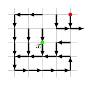
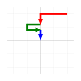
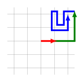
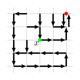
(a)	(b)	(c)	(d)

Figure 2. (a) The pair $(y,\eta)$, with $y$ given by the red bullet and with $\eta$ restricted to $\operatorname{\mathcal{A}}(x)\cup\{x\}$. (b) The trajectory of the word $w_{1}$ (in red), $w_{2}$ (in green), and $w_{3}$ (in blue). (c) The trajectory of the word $w_{4}$ (in red), $w_{5}$ (in green), and $w_{6}$ (in blue). (d) The final pair $(y_{|w|},\eta_{|w|})$. Note that $\eta_{|w|}(y)=\eta(y)$ and $\eta_{|w|}(x)\neq\eta(x)$ as required by Lemma 7.5.

Now note that $w=w_{1}\ldots w_{6}$ is an admissible path for $(y,\eta)$ since it is a concatenation of admissible paths. Also note that

$$y_{|w|}\ =\ y^{(5)}_{|w_{6}|}\ =\ y\hskip 1.70709pt;\qquad\text{ and }\qquad\eta_{|w|}(y)\ =\ \eta^{(5)}_{|w_{6}|}(y)\ =\ \eta(y)\hskip 1.70709pt.$$

Furthermore note that $w\in\operatorname{\mathcal{A}}(x)\cup\{x\}$ by construction, and $x$ occurs exactly once in $w$ (namely as $w_{3}$). Finally note that the length of $w$ satisfies

$$|w|\quad=\quad\sum_{i=1}^{6}|w_{1}|\quad\leq\quad 15\hskip 1.70709pt+\hskip 1.70709pt6\hskip 1.70709pt+\hskip 1.70709pt1\hskip 1.70709pt+\hskip 1.70709pt1\hskip 1.70709pt+\hskip 1.70709pt25\hskip 1.70709pt+\hskip 1.70709pt10\quad=\quad 58\hskip 1.70709pt.$$

This proves the lemma. ∎

Let $\rho$ be an arbitrary rotor configuration. We denote by  $J(\rho):=J(\rho,k,r)$  the set of admissible paths $w=x_{1}\ldots x_{m}$ for $((0,0),\rho)$, such that, exactly one of the following scenarios occur:

(Tau) $$\begin{split}&\text{$x_{m}=(0,0)$, and $(0,0)$ occurs in $w$ exactly $k$ times; or}\\ &\text{$x_{m}\in\partial B_{r}$, and all other vertices in $w$ are not contained in $\partial B_{r}$\hskip 1.70709pt.}\end{split}$$

Described in words,  $J(\rho)$  consists of words that record the feasible locations of the walker until the hitting time $\tau$, for the $\operatorname{\mathcal{H}}$–$\operatorname{\mathcal{V}}$ walk with initialization $((0,0),\rho)$.

We denote by  $J_{0}(\rho,x):=J_{0}(\rho,x,k,r)$  the set of words $w$ in $J(\rho)$ such that $x$ never occurs in $w$, and by  $J_{1}(\rho,x):=J_{1}(\rho,x,k,r)$  the set of words $w$ in $J(\rho)$ such that $x$ occurs at least once in $w$. We now define the map  $\phi:J_{1}(\rho,x)\to J_{1}(\rho,x)$  as follows:

• Let  $w=y_{1}\ldots y_{m}\in J_{1}(\rho,x)$ . Since $x$ occurs at least once in $w$, it follows that some vertex in $\operatorname{\mathcal{D}}(x)$ also occurs at least once in $w$. Let $\ell:=\ell(w)$ be the largest integer such that $y_{\ell}\in\operatorname{\mathcal{D}}(x)$ . Note that  $\{y_{\ell+1},\ldots,y_{m}\}\hskip 0.85355pt\cap\hskip 0.85355pt(\operatorname{\mathcal{A}}(x)\cup\{x\})=\varnothing$  and  $x\in B_{r-3}\setminus B_{3}$.

• We define  $w_{1}\hskip 1.70709pt:=\hskip 1.70709pty_{1}y_{2}\ldots y_{\ell}$  and  $w_{3}\hskip 1.70709pt:=\hskip 1.70709pty_{\ell+1}y_{\ell+2}\ldots y_{m}$ .

• Let  $(y^{\prime},\eta^{\prime}):=(y_{\ell},\eta_{\ell})$  (with respect to the word $w_{1}$ and initialization  $(y_{0},\eta_{0})=((0,0),\rho)$) . Note that $y^{\prime}\in\operatorname{\mathcal{D}}(x)$ by definition. We define $w_{2}$ to be an admissible path for $(y^{\prime},\eta^{\prime})$ such that  $y^{\prime}_{|w_{2}|}=y^{\prime}$  and  $\eta^{\prime}_{|w_{2}|}(y^{\prime})=\eta^{\prime}(y^{\prime})$ . We also require that  $w\in\operatorname{\mathcal{A}}(x)\cup\{x\}$  and that $x$ occurs exactly once in $w$. Such a word $w_{2}$ exists and $|w_{2}|\leq 58$ by Lemma 7.5 .

• We define $\phi(w):=w_{1}w_{2}w_{3}$ .

Lemma 7.6.

For every  $w\in J_{1}(\rho,x)$ , we have that $\phi(w)$ is contained in $J_{1}(\rho,x)$. Furthermore, x occurs in $\phi(w)$ exactly one more time than in $w$, and  $|\phi(w)|\hskip 1.70709pt\leq\hskip 1.70709pt|w|+58$ .

Proof.

We first show that $\phi(w)$ is an admissible path for $((0,0),\rho)$ . First we have $w_{1}$ is an admissible path for $((0,0),\rho)$ by definition, and $w_{2}$ is an admissible path for  $(y^{\prime},\eta^{\prime})$ . We write  $(y^{\prime\prime},\eta^{\prime\prime}):=(y^{\prime}_{|w_{2}|},\eta^{\prime}_{|w_{2}|})$ . Now note that  $y^{\prime\prime}$ is equal to  $y^{\prime}$ , and  $\eta^{\prime}$ agrees with $\eta^{\prime\prime}$ on every vertex outside of  $\operatorname{\mathcal{A}}(x)\cup\{x\}$ . Also note that $w_{3}$ is an admissible path for $(y^{\prime},\eta^{\prime})$, and none of the vertices in  $\operatorname{\mathcal{A}}(x)\cup\{x\}$  occurs in $w_{3}$ (by the maximality of $\ell$). It then follows from these two observations that $w_{3}$ is an admissible path for  $(y^{\prime\prime},\eta^{\prime\prime})$ . Hence  $\phi(w)=w_{1}w_{2}w_{3}$  is a concatenation of admissible paths, and we conclude $\phi(w)$ is an admissible path for $((0,0),\rho)$ .

We now show that $\phi(w)$ satisfies (Tau). Indeed, note that  $\operatorname{\mathcal{A}}(x)\cup\{x\}$  contains neither the origin nor vertices from $\partial B_{r}$ , since $x\in B_{r-3}\setminus B_{3}$. Also note that  $w=w_{1}w_{3}$  satisfies (Tau) by assumption. It then follows from these two observations that  $\phi(w)=w_{1}w_{2}w_{3}$  satisfies (Tau).

Now note that, $x$ occurs in $\phi(w)=w_{1}w_{2}w_{3}$ exactly one more time than in $w=w_{1}w_{3}$, since, $x$ occurs exactly once in $w_{2}$. Also note that

$$|\phi(w)|\quad=\quad|w_{1}|+|w_{2}|+|w_{3}|\quad\leq\quad|w_{1}|+58+|w_{3}|\quad=\quad|w|+58\hskip 1.70709pt.$$

This completes the proof of the lemma. ∎

Lemma 7.7.

Let  $w\in\phi\big{(}J_{1}(x,\rho)\big{)}$ . Then the preimage of $w$ under $\phi$ contains at most 58 elements.

Proof.

Let $w=x_{1}\ldots x_{m}$, and let $\ell$ be the largest integer such that  $x_{\ell}\in\operatorname{\mathcal{D}}(x)$ . Let $w^{\prime}$ be an arbitrary element of the preimage of $w$ under $\phi$. It then follows from the construction of $\phi$ that

$$w^{\prime}=x_{1}\ldots x_{\ell-i}\ x_{\ell+1}\ldots x_{m}\qquad\text{ for some }i\in\{1,\ldots,58\}\hskip 1.70709pt.$$

It then follows that the preimage of $w$ under $\phi$ contains at most 58 elements, as desired. ∎

We are now ready to present the proof of Lemma 7.3.

Proof of Lemma 7.3 .

Note that we have

(26) $$p_{even}(\rho,x)\quad =\quad\sum_{\begin{subarray}{c}w\in J_{1}(\rho,x);\\ K_{x}(w)\hskip 1.70709pt\equiv\hskip 1.70709pt0\text{ mod }2\end{subarray}}2^{-|w|};\qquad p_{odd}(\rho,x)\quad=\quad\sum_{\begin{subarray}{c}w\in J_{1}(\rho,x);\\ K_{x}(w)\hskip 1.70709pt\equiv\hskip 1.70709pt1\text{ mod }2\end{subarray}}2^{-|w|}\hskip 1.70709pt,$$

where $K_{x}(w)$ is the number of visits to $x$ by the walk with admissible path $w$. Now note that, by Lemma 7.6,

(27) $$p_{even}(\rho,x)\quad\leq\quad 2^{58}\sum_{\begin{subarray}{c}w\in J_{1}(\rho,x);\\ K_{x}(w)\hskip 1.70709pt\equiv\hskip 1.70709pt0\text{ mod }2\end{subarray}}2^{-|\phi(w)|}\hskip 1.70709pt.$$

On the other hand, again by Lemma 7.6,

(28) $$\{\hskip 1.70709pt\phi(w)\hskip 1.70709pt\mid\hskip 1.70709ptw\in J_{1}(\rho,x)\hskip 1.70709pt;K_{x}(w)\hskip 1.70709pt\equiv\hskip 1.70709pt0\text{ mod }2\hskip 1.70709pt\}\ \subseteq\ \{\hskip 1.70709ptw\in J_{1}(\rho,x)\hskip 1.70709pt\mid\hskip 1.70709ptK_{x}(w)\hskip 1.70709pt\equiv\hskip 1.70709pt1\text{ mod }2\hskip 1.70709pt\}\hskip 1.70709pt,$$

and furthermore each element in the right side of (28) appears at most 58 times in the left side of (28) by Lemma 7.7. Plugging (28) into (27), we get

$$p_{even}(\rho,x)\quad\leq\quad 58\hskip 1.70709pt2^{58}\hskip 1.70709pt\sum_{\begin{subarray}{c}w\in J_{1}(\rho,x);\\ K_{x}(w)\hskip 1.70709pt\equiv\hskip 1.70709pt1\text{ mod }2\end{subarray}}2^{-|w|}\quad=\quad 58\hskip 1.70709pt2^{58}\hskip 1.70709ptp_{odd}(\rho,x)\hskip 1.70709pt.$$

By an analogous argument we also have  $p_{odd}(\rho,x)\ \leq\ 58\hskip 1.70709pt2^{58}\hskip 1.70709ptp_{even}(\rho,x)$ , and the lemma now follows. ∎

7.2. Proof of Lemma 7.2

We will first prove the following lemma.

Lemma 7.8.

Let $r\geq 6$. Then for every  $x\hskip 1.70709pt\in\hskip 1.70709ptB_{r-3}\setminus B_{3}$,

$$\big{|}\operatorname{\mathbb{E}}_{\rho\sim\operatorname{\mathsf{IUD}}}\hskip 1.70709pt\operatorname{\mathbb{P}}\big{[}\zeta_{\tau}(x)=\operatorname{\mathcal{H}}\big{]}\ -\ \operatorname{\mathbb{E}}_{\rho\sim\operatorname{\mathsf{IUD}}}\hskip 1.70709pt\operatorname{\mathbb{P}}\big{[}\zeta_{\tau}(x)=\operatorname{\mathcal{V}}\big{]}\big{|}\quad\leq\quad\left(1-\frac{1}{58\hskip 1.70709pt2^{58}}\right)\hskip 1.70709pt.$$

Proof.

For every rotor configuration $\rho$, we write

$$p_{0}(\rho,x)\quad:=\quad\sum_{w\in J_{0}(\rho,x)}2^{-|w|}\hskip 1.70709pt,$$

the probability that the $\operatorname{\mathcal{H}}$–$\operatorname{\mathcal{V}}$ walk with initial rotor configuration $\rho$ never visits $x$ before terminating (at either the origin or $\partial B_{r}$). In particular, $p_{0}(\rho,x)$ does not depend on the rotor $\rho(x)$ at $x$ since the walker never visits $x$. Now note that,

$$\begin{split}\operatorname{\mathbb{P}}\big{[}\zeta_{\tau}(x)=\operatorname{\mathcal{H}}\big{]}\quad=\quad&\operatorname{\mathbbm{1}}\{\rho(x)\hskip 1.70709pt=\hskip 1.70709pt\operatorname{\mathcal{H}}\}\,p_{o}(\rho,x)\ +\ \operatorname{\mathbbm{1}}\{\rho(x)\hskip 1.70709pt=\hskip 1.70709pt\operatorname{\mathcal{H}}\}\,p_{even}(\rho,x)\\ &+\quad\operatorname{\mathbbm{1}}\{\rho(x)\hskip 1.70709pt=\hskip 1.70709pt\operatorname{\mathcal{V}}\}\,p_{odd}(\rho,x)\hskip 1.70709pt.\end{split}$$

On the other hand, since $p_{o}(\rho,x)$ does not depend on $\rho(x)$,

$$\operatorname{\mathbb{E}}_{\rho\sim\operatorname{\mathsf{IUD}}}\big{[}\operatorname{\mathbbm{1}}\{\rho(x)\hskip 1.70709pt=\hskip 1.70709pt\operatorname{\mathcal{H}}\}\,p_{o}(\rho,x)\big{]}\quad =\quad\operatorname{\mathbb{E}}_{\rho\sim\operatorname{\mathsf{IUD}}}\big{[}\operatorname{\mathbbm{1}}\{\rho(x)\hskip 1.70709pt=\hskip 1.70709pt\operatorname{\mathcal{H}}\}\big{]}\,\operatorname{\mathbb{E}}_{\rho\sim\operatorname{\mathsf{IUD}}}\big{[}p_{o}(\rho,x)\big{]}$$

$$=\quad\frac{1}{2}\hskip 1.70709ptp_{o}(\rho,x)\hskip 1.70709pt.$$

Combining the two observations above, we get

(29) $$\begin{split}\operatorname{\mathbb{E}}_{\rho\sim\operatorname{\mathsf{IUD}}}\hskip 1.70709pt\operatorname{\mathbb{P}}\big{[}\zeta_{\tau}(x)=\operatorname{\mathcal{H}}\big{]}\quad=\quad&\frac{1}{2}\hskip 1.70709ptp_{o}(\rho,x)\ +\ \operatorname{\mathbb{E}}_{\rho\sim\operatorname{\mathsf{IUD}}}\big{[}\operatorname{\mathbbm{1}}\{\rho(x)\hskip 1.70709pt=\hskip 1.70709pt\operatorname{\mathcal{H}}\}\,p_{even}(\rho,x)\big{]}\\ &+\ \operatorname{\mathbb{E}}_{\rho\sim\operatorname{\mathsf{IUD}}}\big{[}\operatorname{\mathbbm{1}}\{\rho(x)\hskip 1.70709pt=\hskip 1.70709pt\operatorname{\mathcal{V}}\}\,p_{odd}(\rho,x)\big{]}\hskip 1.70709pt.\end{split}$$

By an analogous argument, we have

(30) $$\begin{split}\operatorname{\mathbb{E}}_{\rho\sim\operatorname{\mathsf{IUD}}}\hskip 1.70709pt\operatorname{\mathbb{P}}\big{[}\zeta_{\tau}(x)=\operatorname{\mathcal{V}}\big{]}\quad=\quad&\frac{1}{2}\hskip 1.70709ptp_{o}(\rho,x)\ +\ \operatorname{\mathbb{E}}_{\rho\sim\operatorname{\mathsf{IUD}}}\big{[}\operatorname{\mathbbm{1}}\{\rho(x)\hskip 1.70709pt=\hskip 1.70709pt\operatorname{\mathcal{H}}\}\,p_{odd}(\rho,x)\big{]}\\ &+\ \operatorname{\mathbb{E}}_{\rho\sim\operatorname{\mathsf{IUD}}}\big{[}\operatorname{\mathbbm{1}}\{\rho(x)\hskip 1.70709pt=\hskip 1.70709pt\operatorname{\mathcal{V}}\}\,p_{even}(\rho,x)\big{]}\hskip 1.70709pt.\end{split}$$

We now apply Lemma 7.3 to (29), and we get

(31) $$\begin{split}\operatorname{\mathbb{E}}_{\rho\sim\operatorname{\mathsf{IUD}}}\hskip 1.70709pt\operatorname{\mathbb{P}}\big{[}\zeta_{\tau}(x)=\operatorname{\mathcal{H}}\big{]}\quad\geq\quad&\frac{1}{2}\hskip 1.70709ptp_{o}(\rho,x)\ +\ \frac{1}{58\hskip 1.70709pt2^{58}}\hskip 1.70709pt\operatorname{\mathbb{E}}_{\rho\sim\operatorname{\mathsf{IUD}}}\big{[}\operatorname{\mathbbm{1}}\{\rho(x)\hskip 1.70709pt=\hskip 1.70709pt\operatorname{\mathcal{H}}\}\,p_{odd}(\rho,x)\big{]}\\ &+\ \frac{1}{58\hskip 1.70709pt2^{58}}\hskip 1.70709pt\operatorname{\mathbb{E}}_{\rho\sim\operatorname{\mathsf{IUD}}}\big{[}\operatorname{\mathbbm{1}}\{\rho(x)\hskip 1.70709pt=\hskip 1.70709pt\operatorname{\mathcal{V}}\}\,p_{even}(\rho,x)\big{]}\hskip 1.70709pt.\end{split}$$

Taking the difference between (30) and (31), we get

(32) $$\begin{split}&\operatorname{\mathbb{E}}_{\rho\sim\operatorname{\mathsf{IUD}}}\hskip 1.70709pt\operatorname{\mathbb{P}}\big{[}\zeta_{\tau}(x)=\operatorname{\mathcal{V}}\big{]}\ -\ \operatorname{\mathbb{E}}_{\rho\sim\operatorname{\mathsf{IUD}}}\hskip 1.70709pt\operatorname{\mathbb{P}}\big{[}\zeta_{\tau}(x)=\operatorname{\mathcal{H}}\big{]}\\ &\leq\left(1-\frac{1}{58\hskip 1.70709pt2^{58}}\right)\hskip 1.70709pt\bigg{(}\operatorname{\mathbb{E}}_{\rho\sim\operatorname{\mathsf{IUD}}}\big{[}\operatorname{\mathbbm{1}}\{\rho(x)\hskip 1.70709pt=\hskip 1.70709pt\operatorname{\mathcal{H}}\}\,p_{odd}(\rho,x)\big{]}\\ &\phantom{\leq\left(1-\frac{1}{58\hskip 1.70709pt2^{58}}\right)\hskip 1.70709pt\bigg{(}}\ +\ \operatorname{\mathbb{E}}_{\rho\sim\operatorname{\mathsf{IUD}}}\big{[}\operatorname{\mathbbm{1}}\{\rho(x)\hskip 1.70709pt=\hskip 1.70709pt\operatorname{\mathcal{V}}\}\,p_{even}(\rho,x)\big{]}\bigg{)}\hskip 1.70709pt.\end{split}$$

Noting that the last term in (32) is less than the right side of (30), we get

$$\begin{split}&\operatorname{\mathbb{E}}_{\rho\sim\operatorname{\mathsf{IUD}}}\hskip 1.70709pt\operatorname{\mathbb{P}}\big{[}\zeta_{\tau}(x)=\operatorname{\mathcal{V}}\big{]}\ -\ \operatorname{\mathbb{E}}_{\rho\sim\operatorname{\mathsf{IUD}}}\hskip 1.70709pt\operatorname{\mathbb{P}}\big{[}\zeta_{\tau}(x)=\operatorname{\mathcal{H}}\big{]}\quad\leq\quad\left(1-\frac{1}{58\hskip 1.70709pt2^{58}}\right)\hskip 1.70709pt\operatorname{\mathbb{E}}_{\rho\sim\operatorname{\mathsf{IUD}}}\hskip 1.70709pt\operatorname{\mathbb{P}}\big{[}\zeta_{\tau}(x)=\operatorname{\mathcal{V}}\big{]}\hskip 1.70709pt.\end{split}$$

Noting that  $\operatorname{\mathbb{P}}\big{[}\zeta_{\tau}(x)=\operatorname{\mathcal{V}}\big{]}$  is at most equal to 1, we then have

(33) $$\operatorname{\mathbb{E}}_{\rho\sim\operatorname{\mathsf{IUD}}}\hskip 1.70709pt\operatorname{\mathbb{P}}\big{[}\zeta_{\tau}(x)=\operatorname{\mathcal{V}}\big{]}\ -\ \operatorname{\mathbb{E}}_{\rho\sim\operatorname{\mathsf{IUD}}}\hskip 1.70709pt\operatorname{\mathbb{P}}\big{[}\zeta_{\tau}(x)=\operatorname{\mathcal{H}}\big{]}\quad\leq\quad\left(1-\frac{1}{58\hskip 1.70709pt2^{58}}\right)\hskip 1.70709pt.$$

By an analogous argument, we also have

(34) $$\operatorname{\mathbb{E}}_{\rho\sim\operatorname{\mathsf{IUD}}}\hskip 1.70709pt\operatorname{\mathbb{P}}\big{[}\zeta_{\tau}(x)=\operatorname{\mathcal{H}}\big{]}\ -\ \operatorname{\mathbb{E}}_{\rho\sim\operatorname{\mathsf{IUD}}}\hskip 1.70709pt\operatorname{\mathbb{P}}\big{[}\zeta_{\tau}(x)=\operatorname{\mathcal{V}}\big{]}\quad\leq\quad\left(1-\frac{1}{58\hskip 1.70709pt2^{58}}\right)\hskip 1.70709pt.$$

The lemma now follows by combining (33) and (34). ∎

Proof of Lemma 7.2.

We have by the definition of the weight function that

$$\operatorname{\mathbb{E}}_{\rho\sim\operatorname{\mathsf{IUD}}}\hskip 1.70709pt\operatorname{\mathbb{E}}\big{[}\operatorname{\mathsf{wt}}\big{(}x,\tau(\rho)\big{)}\big{]}\quad=\quad\operatorname{\mathbb{E}}_{\rho\sim\operatorname{\mathsf{IUD}}}\hskip 1.70709pt\operatorname{\mathbb{P}}\big{[}\zeta_{\tau}(x)=\operatorname{\mathcal{H}}\big{]}\,\operatorname{\mathsf{f}}_{\operatorname{\mathcal{H}}}(x)\ +\ \operatorname{\mathbb{E}}_{\rho\sim\operatorname{\mathsf{IUD}}}\hskip 1.70709pt\operatorname{\mathbb{P}}\big{[}\zeta_{\tau}(x)=\operatorname{\mathcal{V}}\big{]}\,\operatorname{\mathsf{f}}_{\operatorname{\mathcal{V}}}(x)\hskip 1.70709pt.$$

It then follows from (11) and (19) that

$$\big{|}\operatorname{\mathbb{E}}_{\rho\sim\operatorname{\mathsf{IUD}}}\hskip 1.70709pt\operatorname{\mathbb{E}}\big{[}\operatorname{\mathsf{wt}}\big{(}x,\tau(\rho)\big{)}\big{]}\big{|}\quad=\quad \big{|}\operatorname{\mathbb{E}}_{\rho\sim\operatorname{\mathsf{IUD}}}\hskip 1.70709pt\operatorname{\mathbb{P}}\big{[}\zeta_{\tau}(x)=\operatorname{\mathcal{H}}\big{]}\ -\ \operatorname{\mathbb{E}}_{\rho\sim\operatorname{\mathsf{IUD}}}\hskip 1.70709pt\operatorname{\mathbb{P}}\big{[}\zeta_{\tau}(x)=\operatorname{\mathcal{V}}\big{]}\big{|}|\operatorname{\mathsf{f}}(x)|\hskip 1.70709pt.$$

An application of Lemma 7.8 to the last equation yields (25), as desired. ∎

Proof of Proposition 7.1.

We apply the same calculations as in the proof of Proposition 6.1 but with (25) substituting (23) (with details omitted for brevity), and we get

$$\operatorname{\mathbb{E}}_{\rho\sim\operatorname{\mathsf{IUD}}}\big{[}p_{\operatorname{\textnormal{rec}}}(\rho)\big{]}\quad\geq\quad\frac{1}{58\hskip 1.70709pt2^{58}}\quad>\quad 0\hskip 1.70709pt.$$

It now follows from Proposition 2.10 that  $p_{\operatorname{\textnormal{rec}}}(\rho)\hskip 1.70709pt=\hskip 1.70709pt1$  for almost every rotor configuration $\rho$ sampled from $\operatorname{\mathsf{IUD}}$, as desired. ∎

Proof of Theorem 1.3.

The theorem follows from combining Proposition 6.1 (for the case $q<1$) and Proposition 7.1 (for the case $q=1$). ∎

8. Concluding remarks

8.1. Recurrence of other rotor configurations

The techniques used in this paper is quite robust to changes of the initial rotor configuration, and in some cases one can even get a stronger result for specific rotor configurations, e.g.,

• For $q\in[\frac{1}{2},1]$, the following rotor configuration is recurrent:

  $$\rho_{\text{Box}}(x)\quad:=\quad\begin{cases}x+(0,1)&\text{ if }\arg(x)\in\big{(}-\frac{\pi}{4},\frac{\pi}{4}\big{]};\\ x-(1,0)&\text{ if }\arg(x)\in\big{(}\frac{\pi}{4},\frac{3\pi}{4}\big{]};\\ x-(0,1)&\text{ if }\arg(x)\in\big{(}\frac{3\pi}{4},\pi\big{]}\ \text{ or }\ \arg(x)\in\big{(}-\pi,-\frac{3\pi}{4}\big{]};\\ x+(1,0)&\text{ if }\arg(x)\in\big{(}-\frac{3\pi}{4},-\frac{\pi}{4}\big{]}.\end{cases}$$

• For $q\in(0,\frac{1}{2}]$, the following rotor configuration is recurrent:

  $$\rho_{\text{Line}}(x)\quad:=\quad\begin{cases}x+(1,0)&\text{ if }\arg(x)\in\big{(}-\frac{\pi}{4},\frac{\pi}{4}\big{]};\\ x+(0,1)&\text{ if }\arg(x)\in\big{(}\frac{\pi}{4},\frac{3\pi}{4}\big{]};\\ x-(1,0)&\text{ if }\arg(x)\in\big{(}\frac{3\pi}{4},\pi\big{]}\ \text{ or }\ \arg(x)\in\big{(}-\pi,-\frac{3\pi}{4}\big{]};\\ x-(0,1)&\text{ if }\arg(x)\in\big{(}-\frac{3\pi}{4},-\frac{\pi}{4}\big{]}.\end{cases}$$

See Figure 3 for an illustratrion of  $\rho_{\text{Box}}$,  $\rho_{\text{Line}}$, and  $\rho_{\text{Alternating}}$ . The rotor configuration $\rho_{\text{Box}}$ is notably also a recurrent configuration [AH12] and a configuration with minimal range [FLP16] for the clockwise rotor walk.

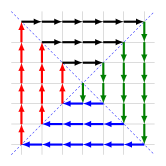
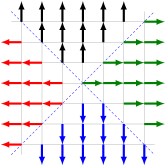
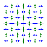
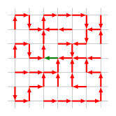
(a)	(b)	(c)	(d)

Figure 3. (a) The configuration $\rho_{\text{Box}}$. (b) The configuration $\rho_{\text{Line}}$. (c) The configuration $\rho_{\text{Alternating}}$. (d) The configuration $\rho_{\text{USTP}}$. Note that, for $\operatorname{\mathcal{H}}$–$\operatorname{\mathcal{V}}$ walks, the up-arrow ($\uparrow$) and the down-arrow ($\downarrow$) is equivalent to the label $\operatorname{\mathcal{V}}$ ($\updownarrow$), while the left-arrow ($\leftarrow$) and the right-arrow ($\rightarrow$) is equivalent to the label $\operatorname{\mathcal{H}}$ ($\leftrightarrow$).

On the other hand, we believe that our results in Theorem 1.1 and Theorem 1.3 are likely not tight. Indeed, the techniques used in the proof of Theorem 1.3 could be used to derive the recurrence for $\operatorname{\mathsf{IID}}$ uniform rotor configuration on the four directions for a slightly larger regime $q\in\big{(}\frac{1}{3}-\varepsilon,1\big{]}$, with  $\varepsilon\hskip 1.70709pt\approx\hskip 1.70709pt1.5\times 10^{-19}$ . In fact, we believe that the following stronger claim is true.

Conjecture 8.1.

Let $q\in(0,1]$. Then, for every initial rotor configuration, the corresponding $\operatorname{\mathcal{H}}$–$\operatorname{\mathcal{V}}$ walk with a single walker is recurrent a.s..

Note that the recurrence regime $q\in(0,1]$ in Conjecture 8.1 is the best one could hope for, as there exist transient rotor configurations when $q=0$ (see Section 8.2 below).

The real obstacle in proving Conjecture 8.1 is the lack of understanding of the law of the rotor configuration $\rho_{t}$ at the $t$-th step of the walk (we speculate on the law of $\rho_{t}$ in Problem 8.2 below). Indeed, with the exception of the proof of Proposition 7.1, we always use the following rudimentary upper bound: for all $t\geq 0$ and $x\in\operatorname{\mathbb{Z}}^{2}$,

$$\big{|}\hskip 1.70709pt\operatorname{\mathbb{P}}[\rho_{t}(x)\ =\ \operatorname{\mathcal{H}}]\ -\ \operatorname{\mathbb{P}}[\rho_{t}(x)\ =\ \operatorname{\mathcal{V}}]\hskip 1.70709pt\big{|}\quad\leq\quad 1\hskip 1.70709pt.$$

Thus developing a better upper bound for the inequality above would (e.g., an $o(1)$ upper bound) constitute a natural first step in solving Conjecture 8.1.

8.2. The case $q=0$

None of our main results apply to $\operatorname{\mathcal{H}}$–$\operatorname{\mathcal{V}}$ walks with $q=0$, as the martingale in Definition 4.3 is not well defined. In fact, there are rotor configurations for this walk that are transient, regardless of the number of walkers (c.f., Theorem 1.1). Indeed, it is straightforward to check that, for $\rho_{\text{Box}}$, each walker visits every vertex only finitely many times. On the other hand, it is straightforward to show that the following rotor configuration is recurrent for this walk:

$$\rho_{\text{Alternating}}(a,b)\ :=\ \begin{cases}\operatorname{\mathcal{H}}&\text{ if }b-a\ \equiv\ 0\text{ mod }2;\\ \operatorname{\mathcal{V}}&\text{ if }b-a\ \equiv\ 1\text{ mod }2,\end{cases}$$

as the even steps of this walk $(X_{2t})_{t\geq 0}$ is a simple random walk on $\operatorname{\mathbb{Z}}^{2}$ with each step being sampled uniformly from $\{(\pm 1,\pm 1)\}$ . (See Figure 3 for an illustration of $\rho_{\text{Alternating}}$.)

Suppose now that $\rho$ is sampled from the $\operatorname{\mathsf{IID}}$ uniform measure on $\{\operatorname{\mathcal{H}},\operatorname{\mathcal{V}}\}$. Then the $\operatorname{\mathcal{H}}$–$\operatorname{\mathcal{V}}$ walk is not recurrent, as there are infinitely many vertices of $\operatorname{\mathbb{Z}}^{2}$ that are visited only finitely many times a.s.. Indeed, this is because $x\in\operatorname{\mathbb{Z}}^{2}$ will never be visited if the following property is satisfied:

$$\rho(x+(1,0))\ =\ \rho(x-(1,0))\ =\ \operatorname{\mathcal{V}};\qquad\rho(x+(0,1))\ =\ \rho(x-(0,1))\ =\ \operatorname{\mathcal{H}}\hskip 1.70709pt,$$

and, by the Borel-Cantelli lemma, there are infinitely many vertices in $\operatorname{\mathbb{Z}}^{2}$ with this property. On the other hand, there always exist some $x\in\operatorname{\mathbb{Z}}^{2}$ for which $x$ is visited infinitely many times by this walk; see the proof in the discussion after Lemma 2.5 in [HS14]. Note that the dichotomy in Lemma 2.3 does not apply here as the corresponding stack is not regular.

8.3. Stationary distribution and scaling limit

Consider the rotor configuration  $\rho_{\text{USTP}}$, where the rotors at  $\operatorname{\mathbb{Z}}^{2}\setminus\{(0,0)\}$  form a (random) uniform spanning tree directed toward the origin (see [Pem91, BLPS01]), and the rotor at the origin is sampled uniformly from the neighbors of the origin, independently from the uniform spanning tree (See Figure 3 for an illustration of $\rho_{\text{USTP}}$). It was shown in [CGLL18, Theorem 1.1] that $\rho_{\text{USTP}}$ is stationary with respect to the scenery process of the single-walker $\operatorname{\mathcal{H}}$–$\operatorname{\mathcal{V}}$ walk. That is, if the initial rotor configuration $\rho_{0}$ is equal to $\rho_{\text{USTP}}$, then the rotor configuration  $\rho_{t}(\cdot-X_{t})$  at the $t$-th step of walk, observed from the viewpoint of the walker, is equal in distribution to $\rho_{\text{USTP}}$ . It remains to be seen if the following stronger claim of stationarity is true.

Problem 8.2.

Let $q>0$. and let  $(X_{t},\rho_{t})_{t\geq 0}$  be an $\operatorname{\mathcal{H}}$–$\operatorname{\mathcal{V}}$ walk with a single walker with an arbitrary initial rotor configuration. Show that that $\rho_{t}(\cdot-X_{t})$ converges weakly to $\rho_{\text{USTP}}(\cdot)$ as $t\to\infty$. That is, for every $x_{1},\ldots,x_{m}\in V$ and every  $d_{1},\ldots,d_{m}\in\{\operatorname{\mathcal{H}},\operatorname{\mathcal{V}}\}$, show that

$$\operatorname{\mathbb{P}}\big{[}\hskip 1.70709pt\rho_{t}(x_{1}-X_{t})=d_{1}\hskip 1.70709pt,\hskip 1.70709pt\ldots\hskip 1.70709pt,\hskip 1.70709pt\rho_{t}(x_{m}-X_{t})=d_{m}\hskip 1.70709pt\big{]}\quad\overset{t\to\infty}{\longrightarrow}\quad\operatorname{\mathbb{P}}\big{[}\hskip 1.70709pt\rho_{\text{USTP}}(x_{1})=d_{1}\hskip 1.70709pt,\hskip 1.70709pt\ldots\hskip 1.70709pt,\hskip 1.70709pt\rho_{\text{USTP}}(x_{m})=d_{m}\hskip 1.70709pt\big{]}\hskip 1.70709pt.$$

The fact that $\rho_{\text{USTP}}$ is stationary was used in [CGLL18, Theorem 1.2] to show that the quenched scaling limit of the $\operatorname{\mathcal{H}}$–$\operatorname{\mathcal{V}}$ walk with the initial rotor configuration $\rho_{\text{USTP}}$ is the standard Brownian motion in $\operatorname{\mathbb{R}}^{2}$. Simulations suggest that we will obtain the same scaling limit when the initial rotor configuration is sampled from the $\operatorname{\mathsf{IID}}$ uniform measure on $\{\operatorname{\mathcal{H}},\operatorname{\mathcal{V}}\}$ (see Figure 1).

Conjecture 8.3.

Let $q>0$, and let  $(X_{t},\rho_{t})_{t\geq 0}$  be an $\operatorname{\mathcal{H}}$–$\operatorname{\mathcal{V}}$ walk with a single walker with the initial rotor configuration $\rho$ sampled from the $\operatorname{\mathsf{IID}}$ uniform measure on $\{\operatorname{\mathcal{H}},\operatorname{\mathcal{V}}\}$. Then the quenched scaling limit for this walk is the standard Brownian motion $(B_{t})_{t\geq 0}$ in $\operatorname{\mathbb{R}}^{2}$ . That is to say, for almost every $\rho$ sampled from the $\operatorname{\mathsf{IID}}$ uniform measure on $\{\operatorname{\mathcal{H}},\operatorname{\mathcal{V}}\}$,

$$\frac{1}{\sqrt{n}}(X_{\lfloor nt\rfloor})_{t\geq 0}\quad\overset{n\to\infty}{\Longrightarrow}\quad(B_{t})_{t\geq 0},$$

with the convergence being the weak convergence in the Skorohod space $D_{\operatorname{\mathbb{R}}^{2}}[0,\infty)$.

Note that the case $q=0$ in Conjecture 8.3 is a special case of the result of Berger and Deuschel  [BD14, Theorem 1.1], who proved a quenched invariance principle for a large family of random walks in random environments (note that the $\operatorname{\mathcal{H}}-\operatorname{\mathcal{V}}$ walk is not a random walk in random environment anymore when $q>0$).

8.4. $p$-rotor walk on $\operatorname{\mathbb{Z}}^{2}$

Unfortunately, the techniques used in this paper are very sensitive to changes to the model. Indeed, consider the $p$-rotor walk on $\operatorname{\mathbb{Z}}^{2}$ (introduced in [HLSH18]), which is an RWLM where, for each step, a walker rotates the rotor of its current location 90-degrees counter-clockwise with probability $p$, and rotates the rotor 90-degrees clockwise with probability $1-p$. Note that we recover the counterclockwise rotor walk when $p=0$, the clockwise rotor walk when $p=1$, and the $\operatorname{\mathcal{H}}$–$\operatorname{\mathcal{V}}$ walk with $q=1$ when $p=\frac{1}{2}$.

Conjecture 8.4.

Let $p\in[0,1]$. Then, for almost every $\rho$ sampled from the $\operatorname{\mathsf{IID}}$ uniform measure on $\{\operatorname{\mathcal{H}},\operatorname{\mathcal{V}}\}$, the corresponding $p$-rotor walk on $\operatorname{\mathbb{Z}}^{2}$ visits every vertex infinitely many times a.s..

This conjecture was answered positively by Theorem 1.3 for the case $p=\frac{1}{2}$. However, the techniques of this paper break down immediately when $p\neq\frac{1}{2}$, as the best upper bound we have for $\operatorname{\mathbb{E}}|\operatorname{\mathsf{wt}}(x,t)|$ (recall (12)) would then have a linear decay rather than a quadratic decay (see (20)), and we need at least a quadratic decay for the proof of Theorem 1.3 to work. Thus developing a better upper bound for $\operatorname{\mathbb{E}}|\operatorname{\mathsf{wt}}(x,t)|$ would constitute a natural first step in proving Conjecture 8.4.

Appendix A Proof of Lemma 2.4

Proof of Lemma 2.4.

For every $x,y\in V$, let $N_{t}(x,y)$ be the total number of departures from $x$ to $y$, by the stack walk with turn order $\operatorname{\mathcal{O}}$, up to time $t$,

$$N_{t}(x,y)\ :=\ \big{|}\{s\in\{1,\ldots,t\}\hskip 1.70709pt\mid\hskip 1.70709ptX_{s-1}^{(i)}=x,\ X_{s}^{(i)}=y,\ \ \text{ for some }i\in\{1,\ldots,n\}\}\big{|}\hskip 1.70709pt,$$

and we write  $N_{\infty}(x,y)\hskip 1.70709pt:=\hskip 1.70709pt\lim_{t\to\infty}N_{t}(x,y)$ . We denote by $N_{t}^{\prime}(x,y)$ and $N_{\infty}^{\prime}(x,y)$ the same numbers for the stack walk with turn order $\operatorname{\mathcal{O}}^{\prime}$. Note that

$$R_{t}(x)\ =\ \sum_{y\in\operatorname{{Ngh}}(x)}N_{t}(x,y);\qquad R_{t}^{\prime}(x)\ =\ \sum_{y\in\operatorname{{Ngh}}(x)}N_{t}^{\prime}(x,y).$$

Thus it suffices to show that, for all $t\geq 0$, we have  $N_{t}(x,y)\hskip 1.70709pt\leq\hskip 1.70709ptN_{\infty}^{\prime}(x,y)$ for all $x,y\in V$.

Suppose to the contrary that the claim is false. Let $t$ be the smallest integer such that the claim is false. Then there are two consequences. Firstly,

(35) $$R_{t-1}(z)\ \leq\ R^{\prime}_{\infty}(z)\quad\text{ for all }z\in V\hskip 1.70709pt.$$

Secondly, there exists $x\in V$ such that,

$$\sum_{y\in\operatorname{{Ngh}}(x)}N_{t}(x,y)\quad=\quad 1\ +\ \sum_{y\in\operatorname{{Ngh}}(x)}N_{\infty}^{\prime}(x,y).$$

This implies two other consequences. Firstly,

(36) $$N_{t-1}(x,y)\ =\ N_{\infty}^{\prime}(x,y)\qquad\text{ for all }y\in\operatorname{{Ngh}}(x)\hskip 1.70709pt.$$

Secondly, there is at least one walker present at $x$ at the end of the $t-1$-th step of the stack walk with turn order $\operatorname{\mathcal{O}}$, i.e.,

(37) $$|\{i\hskip 1.70709pt\mid\hskip 1.70709pt\operatorname{\mathbf{X}}^{(i)}=x\}|\ +\ R_{t-1}(x)\ -\ \sum_{y\in\operatorname{{Ngh}}(x)}N_{t-1}(x,y)\quad\geq\quad 1,$$

where $\operatorname{\mathbf{X}}^{(i)}\in V^{n}$ is the vector that records the initial locations of the walkers.

Plugging (35) and (36) into (37), we get

$$|\{i\hskip 1.70709pt\mid\hskip 1.70709pt\operatorname{\mathbf{X}}^{(i)}=x\}|\ +\ R_{\infty}(x)\ -\ \sum_{y\in\operatorname{{Ngh}}(x)}N^{\prime}_{\infty}(x,y)\quad\geq\quad 1,$$

This means that, excepting the first few finite steps, there is always at least one walker present at $x$ throughout the entirety of the stack walk with turn order $\operatorname{\mathcal{O}}^{\prime}$. Since $\operatorname{\mathcal{O}}^{\prime}$ is regular, this implies that $N_{\infty}^{\prime}(x,y)=\infty$ for some $y\in\operatorname{{Ngh}}(x)$, which contradicts (36), as desired. ∎

Appendix B Proof of Theorem 2.6

We now build toward the proof of Theorem 2.6, which is adapted from [AH12, Theorem 1].

Consider a variant of the (multi-walker) stack walk on a finite graph, where the walkers are immediately frozen when they reach a specified set of sink vertices $Z$ (which is nonempty).

Lemma B.1 (Least action principle [DF91, Proposition 4.1], see also [BL16, Lemma 4.3]).

Consider a stack walk on a finite graph with the initial location $\operatorname{\mathbf{x}}\in V^{n}$, the initial regular stack $\xi$, and the nonempty sink $Z$. Then the stack walk terminates in a finite number of moves. The final position, i.e., the number of frozen walkers on each vertex, the total number of moves, and the total number of visits to each vertex, are independent of the chosen turn order.

We now apply the least action principle to prove increasingly stronger versions of Theorem 2.6 .

Lemma B.2.

Let $x,x^{\prime}\in V$ and let $\xi$ be a regular stack. Then the stack walk with a single walker with initialization $(x,\xi)$ is recurrent if and only if the stack walk with initialization $(x^{\prime},\xi)$ is recurrent.

Proof.

It suffices to prove that if the stack walk started at $x$ is recurrent, then the stack walk started at a neighbor $x^{\prime}$ of $x$ is also recurrent. By (2) it then suffices to prove that, for every $k\geq 0$, the stack walk started at $x^{\prime}$ visits $x$ at least $k$ times.

Let $m:=m(k)$ be the smallest integer such that  $m\geq k-1$  and $\xi(x,m)=x^{\prime}$ . Note that $m$ exists because $\xi$ is regular. Let $S$ be the finite set of vertices visited by the stack walk started at $x$ until it has made $m+1$ returns to $x$. Let $F$ be the finite subgraph of $G$ induced by $S$, with two additional sink vertices $Z=\{z_{1},z_{2}\}$. Let $\xi^{\prime}$ be the stack of $S$ where every card in $\xi$ pointing outside of $S$ is replaced with a card pointing to $z_{1}$, and every card in $\xi$ pointing to $x$ is replaced with a card pointing to $z_{2}$.

We now start a stack walk on $S$ with $m+1$ walkers at $x$, with initial stack $\xi^{\prime}$, and with sink vertices $Z=\{z_{1},z_{2}\}$. We perform the stack walk with the following turn order: In the beginning a walker leaves $x$ and performs stack walk until it reaches $Z$. Each time a walker reaches $Z$, we repeat the same process with another walker at $x$ until all walkers reach $Z$. Note that this multi-walker stack walk on $S$ follows exactly the trajectory of the original stack walk on $G$ started at $x^{\prime}$, and all the walkers in fact reach $z_{2}$ (since the original walk is recurrent). By the least action principle (Lemma B.1), we can perform this stack walk on $S$ using any turn order, and eventually all walkers will reach $z_{2}$.

Now, we choose another turn order for this stack walk on $S$. First let all the $m+1$ walkers take one step, so there is now one walker at each vertex  $\xi(x,i)$ for $i\in\{0,\ldots,m\}$  (including $x^{\prime}$). Now let the walker at $x^{\prime}$ perform stack walk until it gets absorbed at $z_{2}$. Whenever the $i$-th walker ($i\in\{1,\ldots,m+1\}$) is absorbed at $z_{2}$, we repeat the same process with the $i+1$-th walker being the walker at  $\xi(x,i-1)$ , until every walker reaches $z_{2}$. Note that this stack walk on $S$ follow exactly the trajectory of the original stack walk on $G$ started at $x^{\prime}$, and thus we conclude that the latter visits $x$ at least $m+1\geq k$ times, as desired. ∎

Lemma B.3.

Let $\operatorname{\mathbf{x}},\operatorname{\mathbf{x}}^{\prime}\in V^{n}$ and let $\xi$ be a regular stack. Then $(\operatorname{\mathbf{x}},\xi)$ is recurrent if and only if $(\operatorname{\mathbf{x}}^{\prime},\xi)$ is recurrent.

Proof.

It suffices to show that if $\operatorname{\mathbf{x}}$ and $\operatorname{\mathbf{x}}^{\prime}$ differs by exactly one coordinate and $(\operatorname{\mathbf{x}},\xi)$ is recurrent, then $(\operatorname{\mathbf{x}}^{\prime},\xi)$ is recurrent. By Lemma 2.5, we can without loss of generality assume that $\operatorname{\mathbf{x}}$ and $\operatorname{\mathbf{x}}^{\prime}$ differ only at the $n$-th coordinate. We now consider the stack walk with the $n$-th walker removed. That is, let $\operatorname{\mathbf{x}}^{\prime\prime}\in V^{n-1}$ be the vector defined by  $\operatorname{\mathbf{x}}^{\prime\prime}(i)\hskip 1.70709pt:=\hskip 1.70709pt\operatorname{\mathbf{x}}(i)=\operatorname{\mathbf{x}}^{\prime}(i)$  $(i\in\{1,\ldots,n-1\})$ . There are two cases to check.

Firstly, suppose that $(\operatorname{\mathbf{x}}^{\prime\prime},\xi)$ is recurrent. In this case, it follows from Lemma 2.4 that $(\operatorname{\mathbf{x}}^{\prime},\xi)$ is also recurrent.

Secondly, suppose that $(\operatorname{\mathbf{x}}^{\prime\prime},\xi)$ is transient. Let  $(\operatorname{\mathbf{X}}_{t},\xi_{t})_{t\geq 0}$  be the stack walk with initialization $(\operatorname{\mathbf{x}}^{\prime\prime},\xi)$. Since the stack walk is transient, the stack $\xi^{\prime}$ given by $\xi^{\prime}\ :=\ \lim_{t\to\infty}\xi_{t}$ is well defined. Since $(\operatorname{\mathbf{x}},\xi)$ is recurrent, it then follows from Lemma 2.5 that the single-walker stack walk with initialization $(\operatorname{\mathbf{x}}(n),\xi^{\prime})$ is recurrent. By Lemma B.2 this implies that the stack walk with initialization $(\operatorname{\mathbf{x}}^{\prime}(n),\xi^{\prime})$ is recurrent. Finally by Lemma 2.5 again we conclude that $(\operatorname{\mathbf{x}}^{\prime},\xi)$ is recurrent. This completes the proof. ∎

Proof of Theorem 2.6.

It suffices to consider the case when $\xi^{\prime}$ is obtained from $\xi$ by a single popping operation at $x$, i.e., $\xi^{\prime}=\varphi_{x}(\xi)$. By Lemma B.3 we can without loss of generality assume that all the walkers are initially located at one vertex, i.e.,  $\operatorname{\mathbf{x}}=\operatorname{\mathbf{x}}^{\prime}=(x,\ldots,x)$ .

Suppose that $(\operatorname{\mathbf{x}},\xi)$ is recurrent. Let one walker at $x$ performs one step of the stack walk. Then the pair of walkers-and-stack changes to  $(\operatorname{\mathbf{x}}_{1},\xi_{1})$, where

$$\operatorname{\mathbf{x}}_{1}\ :=\ (\xi(x,0),x,\ldots,x);\qquad\xi_{1}\ :=\ \varphi_{x}(\xi)\ =\ \xi^{\prime}\hskip 1.70709pt,$$

and note that $(\operatorname{\mathbf{x}}_{1},\xi_{1})$ is recurrent by the transitivity of recurrence. It now follows from Lemma B.3 that  $(\operatorname{\mathbf{x}}^{\prime},\xi^{\prime})\hskip 1.70709pt=\hskip 1.70709pt(\operatorname{\mathbf{x}}^{\prime},\xi_{1})$  is recurrent, and the proof is complete. ∎

References

- [ABO16] G. Amir, N. Berger, and T. Orenshtein, Zero-one law for directional transience of one dimensional excited random walks, Ann. Inst. Henri Poincaré Probab. Stat. 52 (2016), 47–57.
- [AO16] G. Amir and T. Orenshtein, Excited Mob, Stochastic Process. Appl. 126 (2016), 439–469.
- [ACK14] O. Angel, N. Crawford, and G. Kozma, Localization for linearly edge reinforced random walks, Duke Math. J. 163 (2014), 889–921.
- [AH11] O. Angel and A. E. Holroyd, Rotor walks on general trees, SIAM J. Discrete Math. 25 (2011), 423–446.
- [AH12] O. Angel and A. E. Holroyd, Recurrent rotor-router configurations, J. Comb. 3 (2012), 185–194.
- [BD14] N. Berger, and J.-D. Deuschel, A quenched invariance principle for non-elliptic random walk in i.i.d. balanced random environment, Probab. Theory Related Fields 158 (2014), 91–126.
- [BL16] B. Bond and L. Levine, Abelian networks I. Foundations and examples, SIAM J. Discrete Math. 30 (2016), 856–874.
- [BLPS01] I. Benjamini, R. Lyons, Y. Peres, and O. Schramm, Uniform spanning forests, Ann. Probab. 29 (2001), 1–65.
- [BW03] I. Benjamini and D. B. Wilson, Excited random walk. Electron. Comm. Probab. 8 (2003), 86–92.
- [CD87] D. Coppersmith and P. Diaconis, Random walk with random reinforcement, unpublished (1987).
- [CGLL18] S. H. Chan, L. Greco, L. Levine, and P. Li, Random walks with local memory, 29 pp., J. Stat. Phys. 184 (2021), Article 6, 28 pp
- [Cha19] S. H. Chan, Rotor walks on transient graphs and the wired spanning forest, SIAM J. Discrete Math. 33 (2019), 2369–2393.
- [Cha20] S. H. Chan, A rotor configuration with maximum escape rate, Electron. Commun. Probab. 25 (2020), 5 pp.
- [CL18] S. H. Chan, and L. Levine, Abelian networks IV. Dynamics of nonhalting network, to appear in Mem. Amer. Math. Soc., 95 pp., arXiv:1804.03322.
- [DF91] P. Diaconis and W. Fulton, A growth model, a game, an algebra, Lagrange inversion, and characteristic classes. Rend. Sem. Mat. Univ. Politec. Torino 49 (1991), 95–119.
- [DST15] M. Disertori, C. Sabot, P. Tarrès, Transience of Edge-Reinforced Random Walk, Comm. Math. Phys. 339 (2015), 121–148.
- [Dur19] R. Durrett, Probability: theory and examples (fifth ed.), Camb. Ser. Stat. Probab. Math. 49, Cambridge Univ. Press, 2019.
- [FGLP14] L. Florescu, S. Ganguly, L. Levine, and Y. Peres, Escape rates for rotor walks in , SIAM J. Discrete Math. 28 (2014), 323–334.
- [FLP16] L. Florescu, L. Levine, and Y. Peres, The range of a rotor walk, Amer. Math. Monthly 123 (2016), 627–642.
- [FU96] Y. Fukai and K. Uchiyama, Potential kernel for two-dimensional random walk, Ann. Probab. 24 (1996), 1979–1992.
- [GMV96] G. R. Grimmett, M. V. Menshikov, S. E. Volkov, Random walks in random labyrinths, Markov Process. Related Fields 2 (1996), 69–86.
- [HLM+08] A. E. Holroyd, L. Levine, K. Meszáros, Y. Peres, J. Propp, and D. Wilson, Chip-firing and rotor-routing on directed graphs, in In and out of equilibrium. 2, Progr. Probab. 60, Birkhäuser, Basel (2008), 331–364.
- [HLSH18] W. Huss, L. Levine, and E. Sava-Huss, Interpolating between random walk and rotor walk, Random Structures Algorithms 52 (2018), 263–282.
- [HMSH15] W. Huss, S. Muller, and E. Sava-Huss, Rotor-routing on Galton-Watson trees, Electron. Commun. Probab. 20 (2015), 12 pp.
- [HP10] A. E. Holroyd and J. Propp, Rotor walks and Markov chains, in Algorithmic probability and combinatorics, Contemp. Math. 520, Amer. Math. Soc., Providence (2010), 105–126.
- [HS11] W. Huss and E. Sava, Rotor-router aggregation on the comb, Electron. J. Combin. 18 (2011), 23 pp.
- [HS12] W. Huss and E. Sava, Transience and recurrence of rotor-router walks on directed covers of graphs, Electron. Commun. Probab. 17 (2012), 13 pp.
- [HS14] M. Holmes and T. S. Salisbury, Random walks in degenerate random environments, Canad. J. Math. 66 (2014), 1050–1077.
- [KOS16] G. Kozma, T. Orenshtein, and I. Shinkar, Excited random walk with periodic cookies, Ann. Inst. Henri Poincaré Probab. Stat. 52 (2016), 1023–1049.
- [KP17] E. Kosygina and J. Peterson, Excited random walks with Markovian cookie stacks, Ann. Inst. Henri Poincaré Probab. Stat. 53 (2017), 1458–1497.
- [KZ08] E. Kosygina and M. Zerner, Positively and negatively excited random walks on integers, with branching processes, Electron. J. Probab. 13 (2008), 1952–1979.
- [KZ13] E. Kosygina and M. Zerner, Excited random walks: Results, methods, open problems, Bull. Inst. Math. Acad. Sin. (N.S.) 8 (2013), 105–157.
- [Law91] G. F. Lawler, Intersections of random walks, Probability and its Applications, Birkhäuser Boston, Inc., 1991.
- [LL09] I. Landau and L. Levine, The rotor-router model on regular trees, J. Combin. Theory Ser. A 116 (2009), 421–433.
- [MPRV12] M. Menshikov, S. Popov, A. F. Ramírez, M. Vachkovskaia, On a general many-dimensional excited random walk, Ann. Probab. 40 (2012), 2106–2130.
- [MO17] S. Müller and T. Orenshtein, Infinite excursions of rotor walks on regular trees, Electron. J. Combin. 24 (2017), no. 2, 21 pp.
- [PDDK96] V. Priezzhev, D. Dhar, A. Dhar, and S. Krishnamurthy, Eulerian walkers as a model of self-organized criticality, Phys. Rev. Lett. 77 (1996), 5079–5082.
- [Pem88] R. Pemantle, Phase transition in reinforced random walk and RWRE on trees, Ann. Probab. 16 (1988), 1229–1242.
- [Pem91] R. Pemantle, Choosing a spanning tree for the integer lattice uniformly, Ann. Probab. 19 (1991), 1559–1574.
- [Pem07] R. Pemantle, A survey of random processes with reinforcement, Probab. Surv. 4 (2007), 1–79.
- [Pro03] J. Propp, Random walk and random aggregation, derandomized, online lecture (2003), https://www.microsoft.com/en-us/research/video/random-walk-and-randomaggregation-derandomized/.
- [PT17] R. Pinsky and N. Travers, Transience, recurrence and the speed of a random walk in a site-based feedback environment, Probab. Theory Related Fields 167 (2017), 917–978.
- [ST15] C. Sabot and Pierre Tarrès, Edge-reinforced random walk, Vertex-Reinforced Jump Process and the supersymmetric hyperbolic sigma model, J. Eur. Math. Soc. 17 (2015), 2353–2378.
- [SZ19] C. Sabot, X. Zeng, A random Schrödinger operator associated with the Vertex Reinforced Jump Process on infinite graphs, J. Amer. Math. Soc. 32 (2019), 311–349.
- [Szn04] A.-S. Sznitman, Topics in random walks in random environment, in School and Conference on Probability Theory, Abdus Salam Int. Cent. Theoret. Phys., Trieste, ICTP Lect. Notes, XVII (2004), 203–266.
- [Tót96] B. Tóth, Generalized Ray-Knight theory and limit theorems for self-interacting random walks on , Ann. Probab. 24 (1996), 1324–1367.
- [Tót01] B. Tóth, Self-interacting random motions–a survey, in Random Walks – A Collection of Surveys, Bolyai Soc. Math. Stud. 9, János Bolyai Math. Soc., Budapest (1999), 349–384.
- [Wil91] D. Williams, Probability with martingales. Cambridge Math. Textbooks, Cambridge Univ. Press, 1991.
- [Wil96] D. B. Wilson, Generating random spanning trees more quickly than the cover time, in Proc. 28th STOC, ACM, New York (1996), 296–303.
- [WLB96] I. Wagner, M. Lindenbaum, and A. Bruckstein, Smell as a computational resource–a lesson we can learn from the ant, in Israel Symposium on Theory of Computing and Systems, IEEE Comput. Soc. Press, Los Alamitos (1996), 219–230.
- [Zei04] O. Zeitouni, Random walks in random environment, in Lectures on probability theory and statistics, Lecture Notes in Math. 1837, Springer, Berlin (2004), 189–312.
- [Zer05] M. Zerner, Multi-excited random walks on integers, Probab. Theory Related Fields 133 (2005), 98–112.
- [Zer06] M. Zerner, Recurrence and transience of excited random walks on and strips, Electron. Commun. Probab. 11 (2006), 118–128.