Proposal: JSNS²-II

1 Introduction

This proposal describes the goal and expected sensitivity of the JSNS²-II at J-PARC Materials and Life Science Experimental Facility (MLF).

The JSNS²-II is the second phase of the JSNS² experiment (J-PARC Sterile Neutrino Search at J-PARC Spallation Neutron Source) [1, 2] with two detectors which are located in 24 m and 48 m baselines to improve the sensitivity of the search for sterile neutrinos, especially in the low $\Delta m^{2}$ region, which has been indicated by the global fit of the appearance mode [3]. Note that the experiment with two detectors were proposed in the JSNS² proposal [1], and 25^th J-PARC PAC strongly recommended to make the two detector configuration [4] (2018) as shown in Fig. 1 even though we started the JSNS² with one detector during the first phase.

Figure 1: The 25^th J-PARC PAC’s recommendation.

Based on the J-PARC PAC’s recommendation, the JSNS² collaboration has put a lot of effort in securing the grant, and the Grant-in-Aid for Specially Promoted Research was awarded in 2020. Therefore, the funding is now available to build the second detector.

The JSNS² aims to have a direct test of the LSND experiment [5] using the same neutrino source ($\mu$ Decay-At-Rest), neutrino target (proton), and detection principle (Inverse-Beta-Decay: IBD) but uses the short-pulsed 3 GeV proton beam and Gd-loaded liquid scintillator (GdLS). Therefore, 100 times better signal-to-noise ratio is given compared to the LSND experiment. Please see the reference [2] for more details such as the current setup and sensitivity of the JSNS² experiment.

The approved Proton-On-Target (POT) of the current JSNS² with one detector from the J-PARC PAC is 1.114$\times$10²³ (1 MW $\times$ 3 years), while we aim to have 1 MW $\times$ 5 years for the JSNS²-II. Considering the constraints in the MLF and the Japanese Fire Law, the baseline of the second detector is 48 m from the target. To get a better sensitivity, the second detector which has 35 tons of fiducial weight, locates outside of the MLF as shown in Fig. 2. On the other hand, the current existing detector stays at the location of 24 m baseline even after the second detector construction.

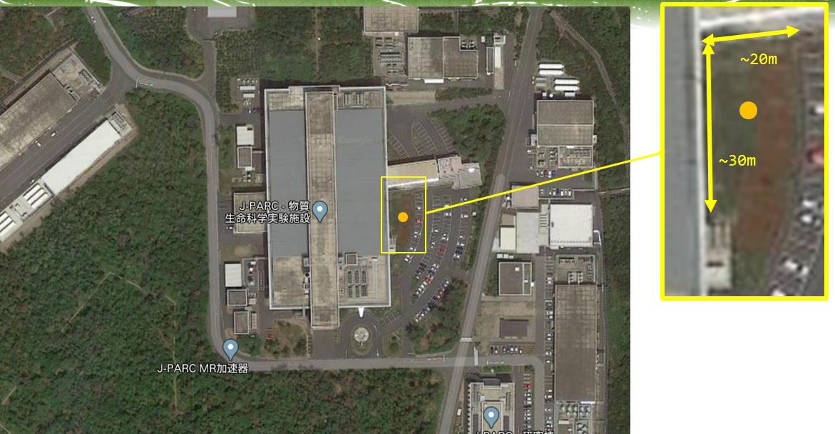
Figure 2: The location of the 2nd detector in the JSNS²-II. The orange circle in the picture shows the location of the detector.

We already started to discuss the issues regarding the Japanese Fire Law and MLF and there have been no show-stoppers thus far.

2 Advantage of two detector configuration

The detector located in the longer baseline can search for the neutrino oscillations with the lower $\Delta m^{2}$ region in general. However, in addition, there are a few large advantages to use two detectors compared to that uses one detector as follows:

1. If sterile neutrinos exist, the observed oscillation pattern as a function of energy will be changed because the neutrino oscillation probability is changed as functions of the flight length and energy of neutrinos as: $P(\bar{\nu_{\mu}}\rightarrow\bar{\nu_{e}})=\sin^{2}2\theta\sin^{2}(\frac{1.27\cdot\Delta m^{2}(eV^{2})\cdot L(m)}{E_{\nu}(MeV)})$. Figure 3 shows the difference of the oscillation probabilities as a function of the energy with two different baselines with the different oscillation parameters.

   

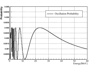
   (a) 24m (LSND best fit)

   

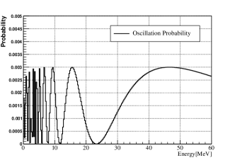
   (b) 48m (LSND best fit)

   

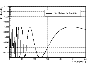
   (c) 24m (JSNS² best fit case)

   

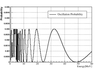
   (d) 48m (JSNS² best fit case)

   Figure 3: Oscillation probabilities at 24 m (left) and 48 m (right) with two different oscillation paramaters. Top: LSND best fit parameters ($\Delta m^{2},sin^{2}(2\theta)$)=(1.2, 0.003), bottom: the JSNS² single detector best fit case. ($\Delta m^{2},sin^{2}(2\theta)$)=(2.5, 0.003)

2. The background rates are different between two detectors because the backgrounds induced from the beam are reduced as a function of distance (1/r²: r is the distance from the mercury target), while backgrounds induced by cosmic rays does not depend on the distance. This makes much better understandings of the backgrounds compared to the one-detector scheme.

3. Systematic uncertainties such as normalization of neutrino fluxes are canceled out using two detectors. This effect will be shown later (section 8).

It might be ideal to use two identical detectors. However JSNS²-II aims to look for the $\bar{\nu}_{\mu}\to\bar{\nu}_{e}$ appearance and the requirements to the systematic uncertainties are relatively small. Therefore, after the detailed understanding of the detector, it is possible to achieve our goals even using the different size detectors.

3 Recent status of sterile neutrino searches

The situation up to 2015 was described in the JSNS² Technical Design Report (TDR) [2]. There have been several new results since then. Here we explain the relevant ones, but please see the reference which reviews them in details [3].

3.1 World-wide status

3.1.1 $\nu_{\mu}\to\nu_{e}$ appearance mode

The MiniBooNE experiment updated their results recently: Their latest publication [6] mentioned that the significance of the $\bar{\nu_{\mu}}\to\bar{\nu_{e}}$ signal compared to background only is 4.7$\sigma$ now. However, as the MicroBooNE experiment [7] pointed out, the observed excess of events in the low-energy region could be due to single $\gamma$ production interactions, which are poorly understood in the current theory, therefore the MiniBooNE cannot distinguish between the oscillation signal and this background because it is a Cherenkov detector. The MicroBooNE uses a liquid argon TPC detector and they can distinguish the oscillation signal and single $\gamma$ events. They are expected to publish their results in near future.

The far detector of the Short Baseline Neutrino experiment (SBN) at FNAL, the ICARUS detector, is ready to take data. They are already fully filled with liquid argon [8], and are waiting for beam. The SBN experiment will provide direct confirmation or refutal of MiniBooNE anormaly.

3.1.2 Disappearance mode

If the neutrino oscillation due to fourth or more mass eigenstates (i.e. sterile neutrino(s)) exist, the $\nu_{e}\to\nu_{s}$ and $\nu_{\mu}\to\nu_{s}$ are also happened accordingly. Especially, three active plus one sterile neutrino model have a simple relationship between appearance and disappearance modes, as shown in our TDR [2] and many other publications (see for example [3]).

For the $\nu_{e}\to\nu_{s}$ searches using the $\nu_{e}$ disappearance, there have been (super-)short baseline reactor experiments, such as Daya-Bay [9], RENO [10], DANSS [11], NEOS [12], Neutrino-4 [13], PROSPECTS [14], Stereo [15]. They typically put the scintillator detectors with the baseline of $\sim$10 meters. The Neutrino-4 experiment declares that they observed a clear oscillation pattern, while other experiments showed the exclusion regions for the two-dimensional mixing angles and $\Delta m^{2}$ plane although some of allowed regions are remained.

$\nu_{\mu}\to\nu_{s}$ searches using the $\nu_{\mu}$ disappearance have been developed by IceCube [16], Super-Kamionkande [17], MINOS/MINOS+ [18] and T2K [19] recently. Their results showed no sterile neutrinos, and there is clear tension between the apperance and the disapperance modes.

3.2 The current JSNS² experiment

Under the current situation, the experiments that provide direct tests for the apperance modes are getting crucial. For the direct test of MiniBooNE, MicroBooNE itself and SBN are important. On the other hand, for the direct test of LSND, the JSNS² plays an important role. The second detector of the JSNS² must be constructed in a timely fashion because the funding to build the second detector was granted in 2020 as recommended by J-PARC PAC.

The JSNS² has started data taking from June 2020 [20]. Currently, we are checking the background rates in the data. We will show some concrete background numbers in the presentation at the next J-PARC PAC.

Currently, we assume that the amount of backgrounds in the second detector is the same as the current one although we expect that they are much smaller backgrounds because the beam-related background, such as gamma rays from MLF third floor concrete, will be reduced drastically compared to the current JSNS² [2].

4 The second detector

The location of the second detector is shown in Fig. 2. In this location, we can have a 8 m $\times$ 8 m space to satisfy the Japanese Fire Law constraint, which requires an empty space of 5 m from the edge of the detector.

The second detector has a similar structure as the existing JSNS² detector, which is already working. The conceptual design of the detector is shown in Fig. 4. As shown here, the detector is placed outside the MLF building and no specific buildings for the detector is made, therefore, we will make a stainless roof on the top of the detector. The electronics, PMT cables and slow monitor/control system are put here.

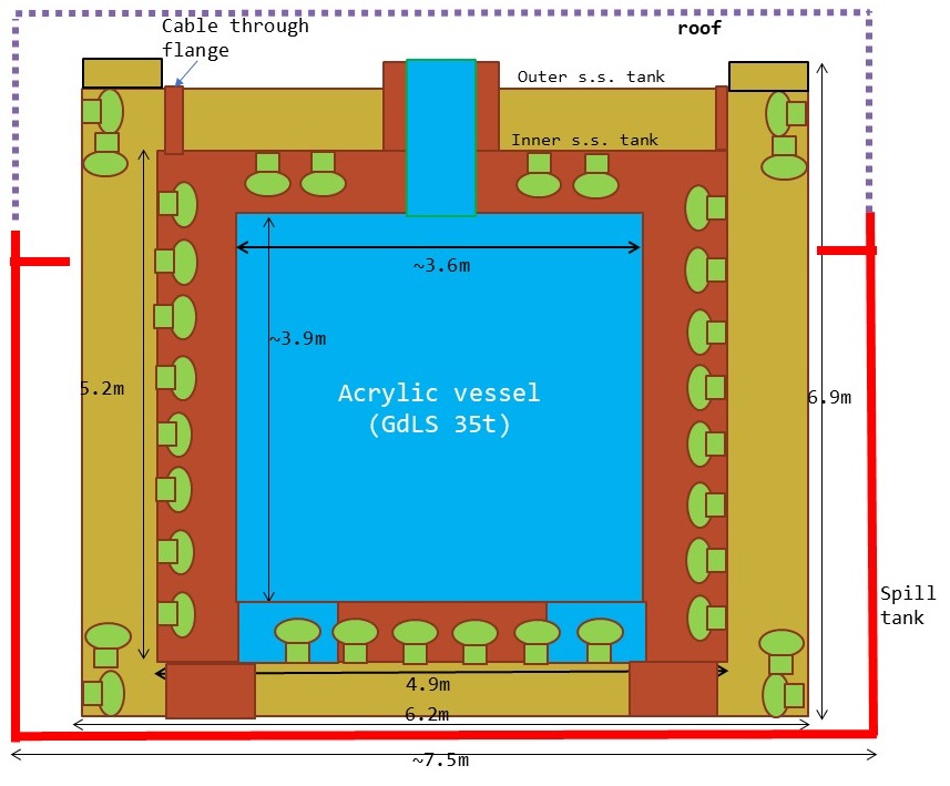
Figure 4: The structure of the 2nd detector in the JSNS²-II.

To compensate for the reduction of the neutrino flux due to the distance from the mercury target, the target mass of the GdLS, which is the Linear AlkylBenzene (LAB) based liquid scintillator, inside the acrylic vessel is increased to 35 tons. On the other hand, the detector located at the longer distance is better at searching in the lower $\Delta m^{2}$ region of the neutrino oscillation.

Similar to reactor experiments such as Daya-Bay [9], RENO [21], Double-Chooz [22], we will have double stainless tank structure. The inner stainless structure makes the sepration of gamma catcher (dark brown) and veto (light brown) regions. In veto region, the same reflector sheets (REIKO LUIREMIRROR [23]) as the existing JSNS² detector will be used. The gamma catcher and veto regions are filled with pure liquid scintillator (LS), which is also based on the LAB. The total weight of the pure LS is about 130 tons.

To keep the same photo coverage of the detector as the first detector, we will surround the acrlyic vessel with the 240 PMTs.

All details of this detector structure will be described in the Technical Design Report (TDR) of the JSNS²-II. Some of GdLS and pure LS (and PMTs if possible) could be donated from the Daya-Bay experiment. The JSNS² has started and will continue to negotiate for this donation.

5 Signal and backgrounds

Based on the JSNS² TDR [2], only the following three data samples must be considered to calculate the sensitivity. Other background components are negligible. The realistic estimation of the background components with the real data taken by the existing detector will be shown in the PAC presentation.

1. signal : $\mu^{+}\to e^{+}+\nu_{e}+\bar{\nu}_{\mu}:\bar{\nu}_{\mu}\to\bar{\nu}_{e}$.

2. intrinsic background : $\mu^{-}\to e^{-}+\nu_{\mu}+\bar{\nu}_{e}$.

3. accidental backgrounds

Hereafter, we will assume that the numbers of events with the event selection efficiency are the same as those in the TDR if the time exposure, detector size, and the baseline of the location are identical, but scaled as function of exposure time and detector fiducial volume for the accidental background, and scaled by 1/r² in addition to the time exposure and detector size, for the intrinsic background.

Table 1 summarizes the number of events in the TDR and those in this proposal configuration. The 1 MW $\times$ 5 years are assumed here to conclude LSND region with 3 sigma confidence level.

	Contents	Current JSNS2	near(24m)	far(48m)
		17tons	17tons	35tons
		5000h/y$\times$3y	5000h/y$\times$5y	5000h/y$\times$5y
	$sin^{2}2\theta=3.0\times 10^{-3}$
	$\Delta m^{2}=2.5eV^{2}$	87	145	24
	$sin^{2}2\theta=3.0\times 10^{-3}$
	$\Delta m^{2}=1.2eV^{2}$	62	103	77
	(Best fit values of LSND)
	$\overline{\nu}_{e}$ from $\mu^{-}$	43	72	36
	${}^{12}C(\nu_{e},e^{-})^{12}N_{g.s.}$	3	5	2
background	beam-associated fast n	$\leq$2	$\leq$3	$\leq$2
	Cosmic-induced fast n	negligible	negligible	negligible
	Total accidental events	20	33	67

Table 1: Summary of the number of events based on the reference [2]. Summary of the event rate for 5000 h/y$\times$3 years for one 17-ton detector (left: [2]) and those with 5000 h/y$\times$5 years for the near (24 m) and far (48 m) detectors. Note that the rate of the beam-related background components has been changed as function of the fiducial mass, the exposure time and the distance from the target. Cosmic ray related backgrounds are changed as function of the fiducial mass and exposure time only.

The expected energy spectra of the background will be described in the next section.

6 Energy spectra of signal and backgrounds

As described in the JSNS² proposal [1], the energy spectra of the signal and background are used to separate them. The beam timing can select the neutrino production from muon (plus) decay-at-rest ($\mu$DAR) from others. Note that the Michel spectrum of $\mu$DAR is well known thanks to the huge efforts made by the elementary particle physicists’ so far [24].

To make the fitting templates, we used the official JSNS² simulation (RAT) and reconstruction (JADE) tools. For example, the energy loss in the acrylic vessel is very well simulated using GEANT4 [25].

Figure 5 shows the true $\bar{\nu_{e}}$ energy and reconstructed energy spectra for the signal (with high $\Delta m^{2}$ region). The event vertices are uniformly randomized in the acrylic vessel region of the detector. The difference of the spectra between the true $\bar{\nu_{e}}$ energy and observed reconstructed energy is mainly due to the energy loss in the acrylic vessel. However, some of them are due to IBD interaction [26].

Figure 6 shows the 2D plot between the true positron energy and the true $\bar{\nu_{e}}$ energy (left), and that between the reconstructed energy and the true $\bar{\nu_{e}}$ energy (right). You can see the effects from the IBD neutrino interaction, the energy reconstruction and the energy loss inside the acrylic vessel.

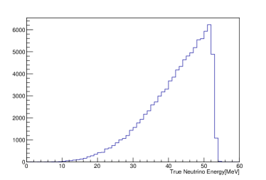
(a) The energy spectrum of signal

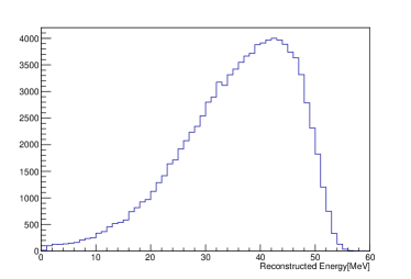
(b) The reconstructed energy of signal events

Figure 5: True $\bar{\nu}_{e}$ energy (left) and the reconstructed energy (right).

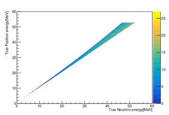
(a) True $\bar{\nu}_{e}$ vs True Positron Energy

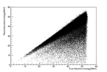
(b) True $\bar{\nu}_{e}$ vs Reconstructed Positron Energy

Figure 6: True energy of $\bar{\nu}_{e}$ (horizontal axis) and true energy of positrons (vertical) simulated one (left). True energy of $\bar{\nu}_{e}$ (horizontal axis) and reconstructed energy of positrons (vertical) (right).

Figure 7 shows the true and reconstructed energy spectra for the intrinsic background ($\bar{\nu}_{e}$ from $\mu^{-}$). Event vertices are uniformly randomized in the acrylic vessel region.

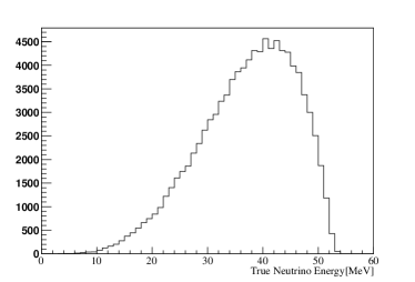
(a) The energy spectrum of intrinsic $\bar{\nu}_{e}$ background

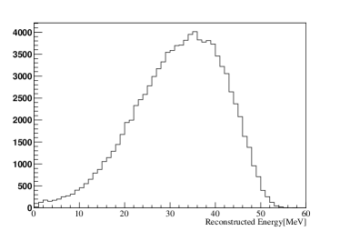
(b) The reconstructed energy

Figure 7: True $\bar{\nu}_{e}$ energy (left) and the reconstructed energy (right).

Figure 8 shows the reconstructed energy spectrum for the accidental background. The background of the prompt IBD region is dominated by the gamma rays induced by cosmic rays. As pointed out by [27], the gamma rays are generated on the surface of the stainless steel tank.

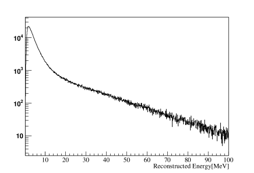
Figure 8: The reconstructed energy of the accidental background.

The expected energy spectra with the LSND best fit parameters of neutrino oscillations ($\Delta m^{2},sin^{2}(2\theta)$)=(1.2, 0.003)) are shown in Fig. 9, The energy spectrum of the $\overline{\nu}_{e}$ generated by the oscillation at 48m baseline is significantly different from that of the intrinsic $\overline{\nu}_{e}$ background.

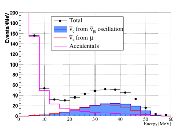
(a) The energy spectrum of 24m detector

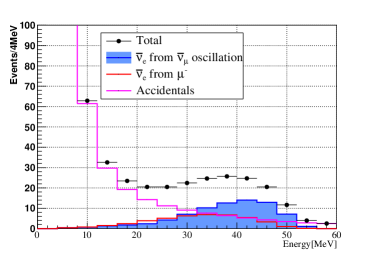
(b) The energy spectrum of 48m detector

Figure 9: Expected observed energy spectrum in the JSNS²-II in two detectors in the LSND best fit case for the 24 m detector (left) and the 48 m detector (right).

7 Fit methods and uncertainties

The important difference between the JSNS² [2] and the JSNS²-II is the ability of JSNS²-II to use different energy spectra information with two different baselines.

Figure 10 shows the expected energy spectra in 24 m detector and 48 m detector for the case with no neutrino oscillations in the JSNS²-II. To make the sensitivity plots, this pseudo-data is used.

As mentioned above, we have two background components. One is from the accidental backgrounds, and the other is from the intrinsic $\bar{\nu}_{e}$ from $\mu^{-}$.

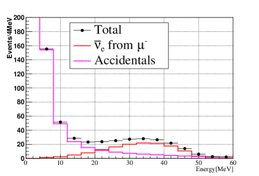
(a) The energy spectrum of 24m detector

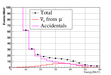
(b) The energy spectrum of 48m detector

Figure 10: Expected observed energy spectrum in the JSNS²-II in two detectors: 24 m detector (left), and 48 m detector (right).

The fitter considers what is the best mixture of the three components among (a) oscillated signal, (b) accidental background, (c) intrinsic $\bar{\nu}_{e}$ from $\mu^{-}$ to explain the energy spectra in Fig. 10. Of course, it is crucial how accurately the normalization factors of these three components are known, therefore the systematic uncertainties of the factors will be discussed later.

7.1 Normalization uncertainty

For the fit of the oscillation parameters, $\Delta m^{2}$ and $\sin^{2}(2\theta)$, constraints of the background normalization are important. However, $\bar{\nu}_{e}$ from $\mu^{-}$ has a very poor normalization constraint from the external information since the production rates of charged pions are not well known due that there have never been any experiments to study the interactions between 3 GeV protons and mercury target. Therefore, 50$\%$ of the uncertainty of the normalization factor for this background is used.

On the other hand, the cross section for the $\nu_{e}+^{12}C\rightarrow e+^{12}N_{gs}$ reaction is known at a 10$\%$ level [28]. The lifetime of $N_{gs}\beta$ decay and the $e^{-}$ energy spectrum are also well known. The measurement of the reaction provides the normalization factor for the oscillated signal ($\bar{\nu_{e}}+p\rightarrow e^{+}+n$) since the parent particle for the oscillated signal is $\bar{\nu_{\mu}}$ from $\mu^{+}$ decays ($\mu^{+}\rightarrow e^{+}+\bar{\nu_{\mu}}+\nu_{e}$). Note that the determination of the normalization factor can be done at the 10$\%$ level.

Finally, the normalization factor of the accidental background can be very well determined by data since the main background of the IBD prompt region is gamma rays induced by the cosmic rays and the IBD delayed background is caused from the beam related gamma rays from the floor and gamma rays induced by the cosmic rays which have small time structure of the rate. So, we don’t need the specific systematic uncertainty on this background normalization.

7.2 Fit method

To get the exclusion region, we use the sum of the backgrounds (intrinsic $\bar{\nu}_{e}$ and accidental backgrounds) as the pseudo-data as mentioned above. In this scheme, the maximum likelihood always obtains $\sin^{2}2\theta$ = 0, regardless of the $\Delta m^{2}$.

7.2.1 Binned likelihood method

A binned maximum likelihood method is used for the analysis. The method fully utilizes the energy spectrum of each background and signal components, thus the amount of the signal components can be estimated efficiently.

For this purpose, the following equation is used.

$$L = L_{1}\times L_{2}$$ (1)

$$= \displaystyle\left[\Pi_{i}P_{1}(N_{exp}|N_{obs})_{i}\right]_{1}\times\left[\Pi_{i}P_{2}(N_{exp}|N_{obs})_{i}\right]_{2}$$ (2)

$$P(N_{exp}|N_{obs}) = \frac{e^{-N_{exp}}\cdot(N_{exp})^{N_{obs}}}{N_{obs}!}$$ (3)

where, $L_{1}$ and $L_{2}$ are the likelihoods of the first and second detectors, the index $i$ refers to the $i$-th energy bin, $N_{exp}$ is expected number of events in $i$-th bin, $N_{obs}$ is number of observed events in $i$-th bin. Energies between 20 and 60 MeV are only considered because the energy cut above 20 MeV is applied for the primary signal as explained before. Note that $N_{exp}=N_{sig}(\Delta m^{2},\sin^{2}2\theta)+\displaystyle\sum N_{bkg}$, and $N_{sig}(\Delta m^{2},\sin^{2}2\theta)$ is calculated by the two flavor neutrino oscillation equation as shown before: $P(\bar{\nu_{\mu}}\rightarrow\bar{\nu_{e}})=\sin^{2}2\theta\sin^{2}(\frac{1.27\cdot\Delta m^{2}(eV^{2})\cdot L(m)}{E_{\nu}(MeV)})$.

The maximum likelihood point gives the best fit parameters, and 2$\Delta lnL$ provides the uncertainty of the fit parameters. As shown in the PDG [24], we have to use the 2$\Delta lnL$ for 2 parameter fits to determine the uncertainties from the fit.

7.2.2 Treatment of systematic uncertainties

Equation 1 takes only statistical uncertainty into account, therefore the systematic uncertainties should be incorporated in the likelihood. Fortunately, energy spectrum of the oscillated signal and background components are well known, thus the error (covariance) matrix of energy is not needed. Note that the uncertainty on the energy scale does not affect to the sensitivity if we achieve the 1$\%$ systematic error as described in [29] (See Fig.121 therein).

In this case, the uncertainties of the overall normalization of each component have to be taken into account, and the assumption is a good approximation.

In order to incorporate the systematic uncertainties, the constraint terms should be added to Equation 1 and the equation is changed as follows.

$$L = [\Pi_{i}P(N_{exp}^{{}^{\prime}}|N_{obs})_{i}]\times e^{-\frac{(1-f_{1})^{2}}{2\Delta\sigma_{1}^{2}}}\times e^{-\frac{(1-f_{2})^{2}}{2\Delta\sigma_{2}^{2}}}$$ (4)

where $f_{j}$ are nuisance parameters to give the constraint term on the overall normalization factors. $N_{exp}^{{}^{\prime}}=f_{1}\cdot N_{sig}(\Delta m^{2},\sin^{2}2\theta)+f_{2}\cdot N_{intrinsic\hskip 2.84544ptbkg}+N_{accidental\hskip 2.84544ptbkg}$. $\Delta\sigma_{i}$ gives the uncertainties on the normalization factors of each components. In this proposal, the profiling fitting method is used to treat the systematic uncertainties. The method is widely known as the correct fitting method as well as the marginalizing method. The profiling method fits all nuisance parameters as well as oscillation parameters.

As mentioned above, the flux of the $\bar{\nu}_{e}$ from $\mu^{-}$ decays around the mercury target has very poor constraints from the external information. For this situation, the uncertainty of this background component is assigned to be 50$\%$.

Table 2 shows the summary of the uncertainty of the normalization factors for the signal and background components. They are regarded as inputs of $\Delta\sigma$ although only $\bar{\nu}_{e}$ from $\mu^{-}$ and the accidental background are used as mentioned above.

components	uncertainty	comments
signal	10$\%$	normalized by $\nu_{e}$ from $\mu^{+}$
$\bar{\nu_{e}}$ from $\mu^{-}$	50 $\%$
cosmic / beam	negligible	well known from calibration source

Table 2: Summary of uncertainties on the normalization factors. Note that only $\bar{\nu}_{e}$ from $\mu^{-}$ and accidental backgrounds are used in the fitting since they are dominant ones in TDR.

8 Expected sensitivity

Figure 11 shows the sensitivity of the JSNS²-II. We assume that the starting point of the JSNS²-II is after 3 years of running of the current JSNS² experiment. For the reference, the sensitivity of the current JSNS² experiment [2] is also shown.

The sensitivity becomes better, especially in the low $\Delta m^{2}$ region, which has been indicated by the global fit of the appearance mode [3] because of the longer baseline. The 3$\sigma$ C.L. line nicely covers most of LSND indicated regions.

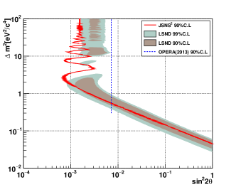
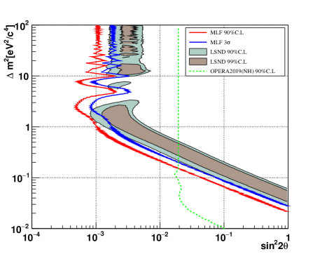
Figure 11: The sensitivity of the JSNS²-II (right). For the comparison, the sensitivity of the current JSNS² is also shown in the left.

To understand the power of the sensitivity of each detector (24 m and 48 m baselines) and combination of the signal and background understanding, Figs. 12 compare the sensitivity with each detector only and JSNS²-II. Below 1 eV², the second detector effects are large as expected. Also we can see the cancellation effects of the systematic uncertainties on the neutrino flux normalizations, espaecially at lower $\Delta m^{2}$. In the lower $\Delta m^{2}$ region, the energy spectra between the oscillation signals and the intrinsic background are getting closer due to the oscillation pattern. In that case, the cancellation effects of the normalization error on the intrinsic background due to two detectors are large.

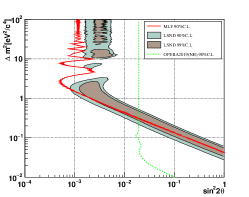
(a) near (24 m)

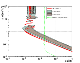
(b) far (48 m)

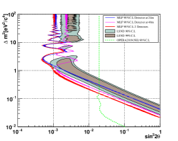
(c) each detector/combined

Figure 12: The sensitivity of the near and the far detectors. (a): the near (24 m) detector only. (b): the far (48 m) detector only. (c): overlaid plots for each detctor and the JSNS²-II.

9 Timescale and cost

The possible timescale of the JSNS²-II is shown in Fig. 13.

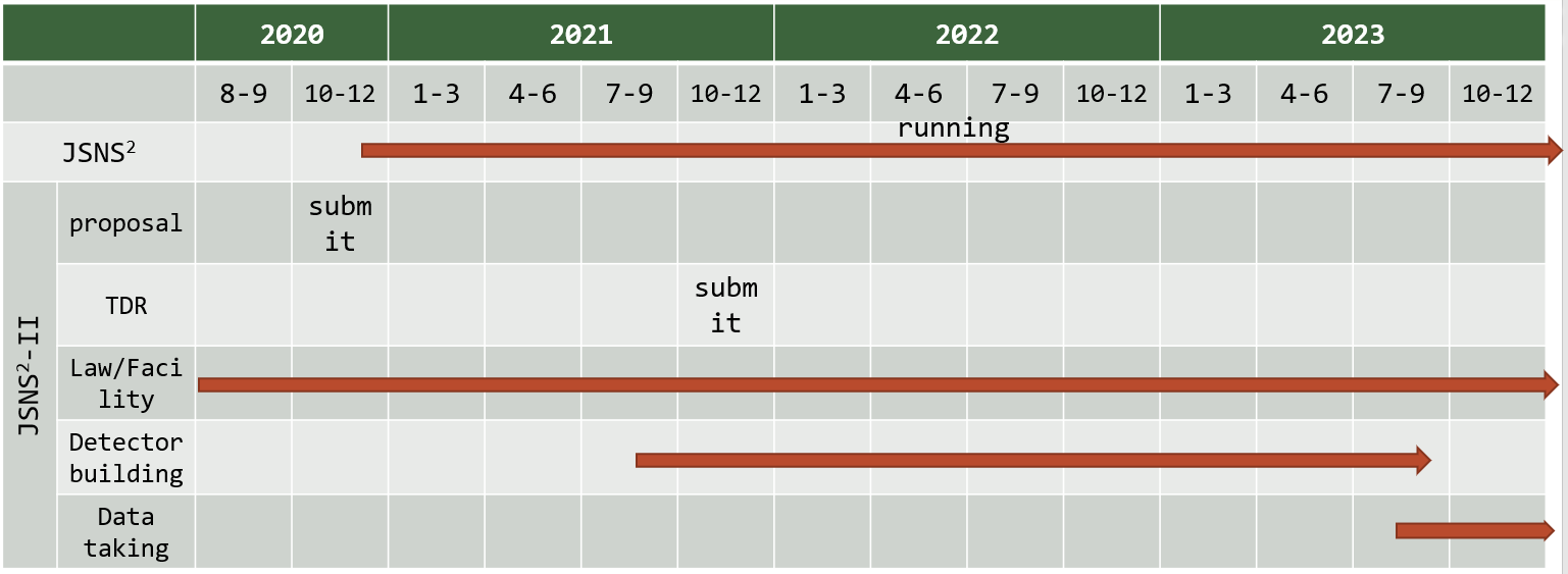
Figure 13: The timescale of the JSNS²-II.

Whilst running the current JSNS² experiment, the second detector will be built, and the JSNS²-II will start data taking from FY2023.

Table 3 shows the cost estimation of the second detector. These numbers are based on the experience of the 1st detector construction. Note that the Grant-in-Aid for Specially Promoted Research in Japan is adpoted in FY2020, therefore 480M Yen was granted to this project. We assume some of components could be donated from the foreign experiment(s) here.

Item	Unit price	Quantity	Total
* PMTs & Electronics system :	500Ky/ch	240 ch	50My
Tanks & Acrylic Vessels :	120My/set		120My
Gd-LS, Buffer-LS			10My
Fluid handling and infrastructure	50My/set	1 set	50My
Miscellaneous			50My
Grand Total			280My

Table 3: Cost estimation (the second (far) detector). Donations from other foreign experiment(s) are assumed.

10 Acknowledements

We thank the J-PARC staff for their support. We acknowledge the support of the Ministry of Education, Culture, Sports, Science, and Technology (MEXT) and the JSPS grants-in-aid (Grant Number 16H06344, 16H03967, 20H05624), Japan. This work is also supported by the National Research Foundation of Korea (NRF) Grant No. 2016R1A5A1004684, 2017K1A3A7A09015973, 2017K1A3A7A09016426, 2019R1A2C3004955, 2016R1D1A3B02010606, 2017R1A2B4011200, 2018R1D1A1B07050425, 2020K1A3A7A0908 0133 and 2020K1A3A7A09080114. Our work has also been supported by a fund from the BK21 of the NRF. The University of Michigan gratefully acknowledges the support of the Heising-Simons Foundation. This work conducted at Brookhaven National Laboratory was supported by the U.S. Department of Energy under Contract DE-AC02-98CH10886. The work of the University of Sussex is supported by the Royal Society grant no.IES\R3\170385

References

- [1] M. Harada, . arXiv:1310.1437 (2013)
- [2] S. Ajimura, . arXiv:1705.08629 (2017)
- [3] M. Dentler, . arXiv:1803.10661 (2018)
- [4] https://j-parc.jp/researcher/Hadron/en/pac_1801/PAC25thMinutes_approved.pdf
- [5] A. Aguilar, . Phys. Rev. D , 112007 (2001).
- [6] A. A. Aguilar-Arevalo . (MiniBooNE Collaboration) Phys. Rev. Lett. , 221801 (2018)
- [7] https://microboone.fnal.gov/
- [8] https://indico.fnal.gov/event/43209/contributions/187821/attachments/130738/159560/Neutrino2020_Betancourt_.pdf
- [9] F. P. An, , Phys. Rev. Lett. 15 151802 (2016).
- [10] J. H. Choi, , arXiv:2006.07782 (2020)
- [11] I. Alekseev , arXiv:1804.04046 (2018)
- [12] Y. Ko , Phys. Rev. Lett. 12 121802 (2017).
- [13] A. P. Serebrov, . arXiv:1809.10561 (2018)
- [14] M. Andriamirado, , arXiv:2006.11210 (2020)
- [15] H. Almazán , Phys. Rev. , 052002
- [16] https://icecube.wisc.edu/news/view/749
- [17] R. Wendell, . Phys. Rev. 092004 (2010)
- [18] P. Adamson, . Phys. Rev. Lett. 9, 091803 (2019)
- [19] K. Abe, . Phys.Rev. 7, 071103 (2019)
- [20] https://indico.fnal.gov/event/43209/contributions/187854/attachments/129166/159526/Neutrino2020_JSNS2_v3.pdf
- [21] J. K. Ahn, . Phys. Rev. Lett. 191802 (2012)
- [22] Y. Abe, . Phys. Rev. Lett. (2012) 131801
- [23] http://www.reiko.co.jp/eng/product_film.html
- [24] https://pdg.lbl.gov/
- [25] https://geant4.web.cern.ch/
- [26] P. Vogel and J. F. Beacom, Phys. Rev. 053003.
- [27] M. Harada, . arXiv:1502.02255 (2015).
- [28] E. Kolbe, K. Langanke, G. Martinez-Pinedo, P .Vogel, J. Phys. G29 2569 (2003)
- [29] https://research.kek.jp/group/mlfnu/JSNS2_rerevisedTDR_180517.pdf