Probabilistic Dependency Graphs

Abstract

We introduce Probabilistic Dependency Graphs (PDGs), a new class of directed graphical models. PDGs can capture inconsistent beliefs in a natural way and are more modular than Bayesian Networks (BNs), in that they make it easier to incorporate new information and restructure the representation. We show by example how PDGs are an especially natural modeling tool. We provide three semantics for PDGs, each of which can be derived from a scoring function (on joint distributions over the variables in the network) that can be viewed as representing a distribution’s incompatibility with the PDG. For the PDG corresponding to a BN, this function is uniquely minimized by the distribution the BN represents, showing that PDG semantics extend BN semantics. We show further that factor graphs and their exponential families can also be faithfully represented as PDGs, while there are significant barriers to modeling a PDG with a factor graph.

1 Introduction

In this paper we introduce yet another graphical tool for modeling beliefs, Probabilistic Dependency Graphs (PDGs). There are already many such models in the literature, including Bayesian networks (BNs) and factor graphs. (For an overview, see (Koller and Friedman 2009).) Why does the world need one more?

Our original motivation for introducing PDGs was to be able capture inconsistency. We want to be able to model the process of resolving inconsistency; to do so, we have to model the inconsistency itself. But our approach to modeling inconsistency has many other advantages. In particular, PDGs are significantly more modular than other directed graphical models: operations like restriction and union that are easily done with PDGs are difficult or impossible to do with other representations. The following examples motivate PDGs and illustrate some of their advantages.

Example 1.

Grok is visiting a neighboring district. From prior reading, she thinks it likely (probability .95) that guns are illegal here. Some brief conversations with locals lead her to believe that, with probility .1, the law prohibits floomps.

The obvious way to represent this as a BN is to use two random variables $F$ and $G$ (respectively taking values $\{f,\smash{\overline{f}}\}$ and $g,\overline{g}$), indicating whether floomps and guns are prohibited. The semantics of a BN offer her two choices: either assume that $F$ and $G$ to be independent and give (unconditional) probabilities of $F$ and $G$, or choose a direction of dependency, and give one of the two unconditional probabilities and a conditional probability distribution. As there is no reason to choose either direction of dependence, the natural choice is to assume independence, giving her the BN on the left of Figure 1.

   

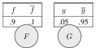
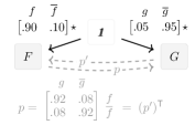
Figure 1: A BN (left) and corresponding PDG (right), which can include more cpds; $p$ or $p^{\prime}$ make it inconsistent.

A traumatic experience a few hours later leaves Grok believing that “floomp” is likely (probability .92) to be another word for gun. Let $p(G\mid F)$ be the conditional probability distribution (cpd) that describes the belief that if floomps are legal (resp., illegal), then with probability .92, guns are as well, and $p^{\prime}(F\mid G)$ be the reverse. Starting with $p$, Grok’s first instinct is to simply incorporate the conditional information by adding $F$ as a parent of $G$, and then associating the cpd $p$ with $G$. But then what should she do with the original probability she had for $G$? Should she just discard it? It is easy to check that there is no joint distribution that is consistent with both the two original priors on $F$ and $G$ and also $p$. So if she is to represent the information with a BN, which always represents a consistent distribution, she must resolve the inconsistency.

However, sorting this out immediately may not be ideal. For instance, if the inconsistency arises from a conflation between two definitions of “gun”, a resolution will have destroyed the original cpds. A better use of computation may be to notice the inconsistency and look up the actual law.

By way of contrast, consider the corresponding PDG. In a PDG, the cpds are attached to edges, rather than nodes of the graph. In order to represent unconditional probabilities, we introduce a unit variable $\mathrlap{\mathit{1}}\mspace{2.3mu}\mathit{1}$ which takes only one value, denoted $\star$. This leads Grok to the PDG depicted in Figure 1, where the edges from $\mathrlap{\mathit{1}}\mspace{2.3mu}\mathit{1}$ to $F$ and $G$ are associated with the unconditional probabilities of $F$ and $G$, and the edges between $F$ and $G$ are associated with $p$ and $p^{\prime}$.

The original state of knowledge consists of all three nodes and the two solid edges from $\mathrlap{\mathit{1}}\mspace{2.3mu}\mathit{1}$. This is like Bayes Net that we considered above, except that we no longer explicitly take $F$ and $G$ to be independent; we merely record the constraints imposed by the given probabilities.

The key point is that we can incorporate the new information into our original representation (the graph in Figure 1 without the edge from $F$ to $G$) simply by adding the edge from $F$ to $G$ and the associated cpd $p$ (the new infromation is shown in blue). Doing so does not change the meaning of the original edges. Unlike a Bayesian update, the operation is even reversible: all we need to do recover our original belief state is delete the new edge, making it possible to mull over and then reject an observation.

The ability of PDGs to model inconsistency, as illustrated in Example 1, appears to have come at a significant cost. We seem to have lost a key benefit of BNs: the ease with which they can capture (conditional) independencies, which, as Pearl (1988) has argued forcefully, are omnipresent.

Example 2 (emulating a BN).

We now consider the classic (quantitative) Bayesian network $\cal B$, which has four binary variables indicating whether a person ($C$) develops cancer, ($S$) smokes, ($\mathit{SH}$) is exposed to second-hand smoke, and ($\mathit{PS}$) has parents who smoke, presented graphically in Figure 2. We now walk through what is required to represent $\cal B$ as a PDG, which we call ${\mathbdcal{M}}_{{\mathcal{B}}}$, shown as the solid nodes and edges in Figure 2.

    

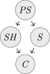
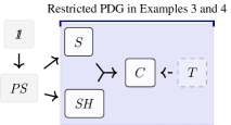
Figure 2: (a) The Bayesian Network $\mathcal{B}$ in Example 2 (left), and (b) ${\mathbdcal{M}}_{\mathcal{B}}$, its corresponding PDG (right). The shaded box indicates a restriction of ${\mathbdcal{M}}_{\mathcal{B}}$ to only the nodes and edges it contains, and the dashed node $T$ and its arrow to $C$ can be added in the PDG, without taking into account $S$ and $SH$.

We start with the nodes corresponding to the variables in $\cal B$, together with the special node $\mathrlap{\mathit{1}}\mspace{2.3mu}\mathit{1}$ from Example 1; we add an edge from ${\mathrlap{\mathit{1}}\mspace{2.3mu}\mathit{1}}$ to $\mathit{PS}$, to which we associate the unconditional probability given by the cpd for $\mathit{PS}$ in $\cal B$. We can also re-use the cpds for $S$ and $\mathit{SH}$, assigning them, respectively, to the edges $PS\to S$ and $PS\to SH$ in ${\mathbdcal{M}}_{{\mathcal{B}}}$. There are two remaining problems: (1) modeling the remaining table in $\cal B$, which corresponds to the conditional probability of $C$ given $S$ and $SH$; and (2) recovering the additional conditional independence assumptions in the BN.

For (1), we cannot just add the edges $S\to C$ and $SH\to C$ that are present in $\cal B$. As we saw in Example 1, this would mean supplying two separate tables, one indicating the probability of $C$ given $S$, and the other indicating the probability of $C$ given $\mathit{SH}$. We would lose significant information that is present in $\cal B$ about how $C$ depends jointly on $S$ and $SH$. To distinguish the joint dependence on $S$ and $\mathit{SH}$, for now, we draw an edge with two tails—a (directed) hyperedge—that completes the diagram in Figure 2. With regard to (2), there are many distributions consistent with the conditional marginal probabilities in the cpds, and the independences presumed by $\cal B$ need not hold for them. Rather than trying to distinguish between them with additional constraints, we develop a a scoring-function semantics for PDGs which is in this case uniquely minimized by the distribution specified by ${\mathcal{B}}$ (LABEL:thm:bns-are-pdgs). This allows us to recover the semantics of Bayesian networks without requiring the independencies that they assume.

Next suppose that we get information beyond that captured by the original BN. Specifically, we read a thorough empirical study demonstrating that people who use tanning beds have a 10% incidence of cancer, compared with 1% in the control group (call the cpd for this $p$); we would like to add this information to $\cal B$. The first step is clearly to add a new node labeled $T$, for “tanning bed use”. But simply making $T$ a parent of $C$ (as clearly seems appropriate, given that the incidence of cancer depends on tanning bed use) requires a substantial expansion of the cpd; in particular, it requires us to make assumptions about the interactions between tanning beds and smoking. The corresponding PDG, ${\mathbdcal{M}}_{{\mathcal{B}}}$, on the other hand, has no trouble: We can simply add the node $T$ with an edge to $C$ that is associated with $\mathbf{p}$. But note that doing this makes it possible for our knowledge to be inconsistent. To take a simple example, if the distribution on $C$ given $S$ and $H$ encoded in the original cpd was always deterministically “has cancer” for every possible value of $S$ and $H$, but the distribution according to the new cpd from $T$ was deterministically “no cancer”, the resulting PDG would be inconsistent.

We have seen that we can easily add information to PDGs; removing information is equally painless.

Example 3 (restriction).

After the Communist party came to power, children were raised communally, and so parents’ smoking habits no longer had any impact on them. Grok is reading her favorite book on graphical models, and she realizes that while the node $\mathit{PS}$ in Figure 2 has lost its usefulness, and nodes $S$ and $\mathit{SH}$ no longer ought to have $\mathit{PS}$ as a parent, the other half of the diagram—that is, the node $C$ and its dependence on $S$ and $\mathit{SH}$—should apply as before. Grok has identified two obstacles to modeling deletion of information from a BN by simply deleting nodes and their associated cpds. First, this restricted model is technically no longer a BN (which in this case would require unconditional distributions on $S$ and $\mathit{SH}$), but rather a conditional BN (Koller and Friedman 2009), which allows for these nodes to be marked as observations; observation nodes do not have associated beliefs. Second, even regarded as a conditional BN, the result of deleting a node may introduce new independence information, incompatible with the original BN. For instance, by deleting the node $B$ in a chain $A\rightarrow B\rightarrow C$, one concludes that $A$ and $C$ are independent, a conclusion incompatible with the original BN containing all three nodes. PDGs do not suffer from either problem. We can easily delete the nodes labeled 1 and $PS$ in Figure 2 to get the restricted PDG shown in the figure, which captures Grok’s updated information. The resulting PDG has no edges leading to $S$ or $\mathit{SH}$, and hence no distributions specified on them; no special modeling distinction between observation nodes and other nodes are required. Because PDGs do not directly make independence assumptions, the information in this fragment is truly a subset of the information in the whole PDG.

Being able to form a well-behaved local picture and restrict knowledge is useful, but an even more compelling reason to use PDGs is their ability to aggregate information.

Example 4.

Grok dreams of becoming Supreme Leader ($\it SL$), and has come up with a plan. She has noticed that people who use tanning beds have significantly more power than those who don’t. Unfortunately, her mom has always told her that tanning beds cause cancer; specifically, that 15% of people who use tanning beds get it, compared to the baseline of 2%. Call this cpd $q$. Grok thinks people will make fun of her if she uses a tanning bed and gets cancer, making becoming Supreme Leader impossible. This mental state is depicted as a PDG on the left of Figure 3.

Grok is reading about graphical models because she vaguely remembers that the variables in Example 2 match the ones she already knows about. When she finishes reading the statistics on smoking and the original study on tanning beds (associated to a cpd $\mathbf{p}$ in Example 2), but before she has time to reflect, we can represent her (conflicted) knowledge state as the union of the two graphs, depicted graphically on the right of Figure 3.

        

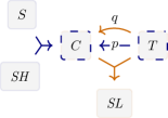
Figure 3: Grok’s prior (left) and combined (right) knowledge.

The union of the two PDGs, even with overlapping nodes, is still a PDG. This is not the case in general for BNs. Note that the PDG that Grok used to represent her two different sources of information (the mother’s wisdom and the study) regarding the distribution of $C$ is a multigraph: there are two edges from $T$ to $C$, with inconsistent information. Had we not allowed multigraphs, we would have needed to choose between the two edges, or represent the information some other (arguably less natural) way. As we are already allowing inconsistency, merely recording both is much more in keeping with the way we have handled other types of uncertainty.

Not all inconsistencies are equally egregious. For example, even though the cpds $p$ and $q$ are different, they are numerically close, so, intuitively, the PDG on the right in Figure 3 is not very inconsistent. Making this precise is the focus of Section 3.2.

These examples give a taste of the power of PDGs. In the coming sections, we formalize PDGs and relate them to other approaches.

2 Syntax

We now provide formal definitions for PDGs. Although it is possible to formalize PDGS with hyperedges directly, we opt for a different approach here, in which PDGs have only regular edges, and hyperedges are captured using a simple construction that involves adding an extra node.

Definition 2.1.

A Probabilistic Dependency Graph is a tuple $\mathbdcal{M}=(\mathcal{N},\mathcal{E},\mathcal{V},\mathbf{p},\alpha,\beta)$, where

$\mathcal{N}$

is a finite set of nodes, corresponding to variables;

$\mathcal{E}$

is a set of labeled edges $\{X\!\overset{\smash{\mskip-5.0mu\raisebox{-1.0pt}{$\scriptscriptstyle L$}}}{\rightarrow}\!Y\}$, each with a source $X$ and target $Y$ in $\mathcal{N}$;

$\mathcal{V}$

associates each variable $N\in\mathcal{N}$ with a set $\mathcal{V}(N)$ of values that the variable $N$ can take;

$\mathbf{p}$

associates to each edge $X\!\overset{\smash{\mskip-5.0mu\raisebox{-1.0pt}{$\scriptscriptstyle L$}}}{\rightarrow}\!Y\in\mathcal{E}$ a distribution $\mathbf{p}_{\!{}_{L}\!}(x)$ on $Y$ for each $x\in\mathcal{V}(X)$;

$\alpha$

associates to each edge $X\!\overset{\smash{\mskip-5.0mu\raisebox{-1.0pt}{$\scriptscriptstyle L$}}}{\rightarrow}\!Y$ a non-negative number $\alpha_{L}$ which, roughly speaking, is the modeler’s confidence in the functional dependence of $Y$ on $X$ implicit in $L$;

$\beta$

associates to each edge $L$ a positive real number $\beta_{L}$, the modeler’s subjective confidence in the reliability of $\mathbf{p}_{\!{}_{L}\!}$.

Note that we allow multiple edges in $\mathcal{E}$ with the same source and target; thus $(\mathcal{N},\mathcal{E})$ is a multigraph. We occasionally write a PDG as $\mathbdcal{M}=(\mathcal{G},\mathbf{p},\alpha,\beta)$, where $\mathcal{G}=(\mathcal{N},\mathcal{E},\mathcal{V})$, and abuse terminology by referring to $\mathcal{G}$ as a multigraph. We refer to ${\mathbdcal{N}}=(\mathcal{G},\mathbf{p})$ as an unweighted PDG, and give it semantics as though it were the (weighted) PDG $(\mathcal{G},\mathbf{p},\mathbf{1},\mathbf{1})$, where $\bf 1$ is the constant function (i.e., so that $\alpha_{L}=\beta_{L}=1$ for all $L$). In this paper, with the exception of Section 4.3, we implicitly take $\alpha={\bf 1}$ and omit $\alpha$, writing $\mathbdcal{M}=(\mathcal{G},\mathbf{p},\beta)$.

If $\mathbdcal{M}$ is a PDG, we reserve the names $\mathcal{N}^{\mathbdcal{M}},\mathcal{E}^{\mathbdcal{M}},\ldots$, for the components of $\mathbdcal{M}$, so that we may reference one without naming them all explicitly. We write $\mathcal{V}(S)$ for the set of possible joint settings of a set $S$ of variables, and write $\mathcal{V}(\mathbdcal{M})$ for all settings of the variables in $\mathcal{N}^{\mathbdcal{M}}$; we refer to these settings as “worlds”. While the definition above is sufficient to represent the class of all legal PDGs, we often use two additional bits of syntax to indicate common constraints: the special variable $\mathrlap{\mathit{1}}\mspace{2.3mu}\mathit{1}$ such that $\mathcal{V}(\mathrlap{\mathit{1}}\mspace{2.3mu}\mathit{1})=\{\star\}$ from Examples 1 and 2, and double-headed arrows, $A\rightarrow\mathrel{\mspace{-15.0mu}}\rightarrow B$, which visually indicate that the corresponding cpd is degenerate, effectively representing a deterministic function $f:\mathcal{V}(A)\to\mathcal{V}(B)$.

Construction 2.2.

We can now explain how we capture the multi-tailed edges that were used in Examples 2 to 4. That notation can be viewed as shorthand for the graph that results by adding a new node at the junction representing the joint value of the nodes at the tails, with projections going back. For instance, the diagram displaying Grok’s prior knowledge in Example 4, on the left of Figure 3 is really shorthand for the following PDG, where where we insert a node labeled $C\times T$ at the junction:

As the notation suggests, $\mathcal{V}(C\times T)=\mathcal{V}(C)\times\mathcal{V}(T)$. For any joint setting $(c,t)\in\mathcal{V}(C\times T)$ of both variables, the cpd for the edge from $C\times T$ to $C$ gives probability 1 to $c$; similarly, the cpd for the edge from $C\times T$ to $T$ gives probability 1 to $t$.

3 Semantics

Although the meaning of an individual cpd is clear, we have not yet given PDGs a “global” semantics. We discuss three related approaches to doing so. The first is the simplest: we associate with a PDG the set of distributions that are consistent with it. This set will be empty if the PDG is inconsistent. The second approach associates a PDG with a scoring function, indicating the fit of an arbitrary distribution $\mu$, and can be thought of as a weighted set of distributions (Halpern and Leung 2015). This approach allows us to distinguish inconsistent PDGs, while the first approach does not. The third approach chooses the distributions with the best score, typically associating with a PDG a unique distribution.

3.1 PDGs As Sets Of Distributions

We have been thinking of a PDG as a collection of constraints on distributions, specified by matching cpds. From this perspective, it is natural to consider the set of all distributions that are consistent with the constraints.

Definition 3.1.

If $\mathbdcal{M}$ is a PDG (weighted or unweighted) with edges $\mathcal{E}$ and cpds $\mathbf{p}$, let $[\mspace{-3.5mu}[\mathbdcal{M}]\mspace{-3.5mu}]_{\text{sd}}$ be the set of distributions over the variables in $\mathbdcal{M}$ whose conditional marginals are exactly those given by $\mathbf{p}$. That is, $\mu\in[\mspace{-3.5mu}[\mathbdcal{M}]\mspace{-3.5mu}]_{\text{sd}}$ iff, for all edges $L\in\mathcal{E}$ from $X$ to $Y$, $x\in\mathcal{V}(X)$, and $y\in\mathcal{V}(Y)$, we have that $\mu(Y\!=\!y\mid X\!=\!x)=\mathbf{p}_{\!{}_{L}\!}(x)$. $\mathbdcal{M}$ is inconsistent if $[\mspace{-3.5mu}[\mathbdcal{M}]\mspace{-3.5mu}]_{\text{sd}}=\emptyset$, and consistent otherwise.

Note that $[\mspace{-3.5mu}[\mathbdcal{M}]\mspace{-3.5mu}]_{\text{sd}}$ is independent of the weights $\alpha$ and $\beta$.

3.2 PDGs As Distribution Scoring Functions

We now generalize the previous semantics by viewing a PDG $\mathbdcal{M}$ as a scoring function that, given an arbitrary distribution $\mu$ on $\mathcal{V}(\mathbdcal{M})$, returns a real-valued score indicating how well $\mu$ fits $\mathbdcal{M}$. Distributions with the lowest (best) scores are those that most closely match the cpds in $\mathbdcal{M}$, and contain the fewest unspecified correlations.

We start with the first component of the score, which assigns higher scores to distributions that require a larger perturbation in order to be consistent with $\mathbdcal{M}$. We measure the magnitude of this perturbation with relative entropy. In particular, for an edge $X\!\overset{\smash{\mskip-5.0mu\raisebox{-1.0pt}{$\scriptscriptstyle L$}}}{\rightarrow}\!Y$ and $x\in\mathcal{V}(X)$, we measure the relative entropy from $\mathbf{p}_{\!{}_{L}\!}(x)$ to $\mu(Y\!=\cdot\mid X=x)$, and take the expectation over $\mu_{X}$ (that is, the marginal of $\mu$ on $X$). We then sum over all the edges $L$ in the PDG, weighted by their reliability.

Definition 3.2.

For a PDG $\mathbdcal{M}$, the incompatibility of a a joint distribution $\mu$ over $\mathcal{V}(\mathbdcal{M})$, is given by

$$\mathit{Inc}_{\mathbdcal{M}}(\mu):=\!\!\!\!\!\!\sum_{X\,\!\overset{\smash{\mskip-5.0mu\raisebox{-1.0pt}{$\scriptscriptstyle L$}}}{\rightarrow}\!\,Y\in\mathcal{E}^{\mathbdcal{M}}}\!\!\!\!\!\beta_{L}^{\mathbdcal{M}}\operatorname*{\mathbb{E}}_{x\sim\mu_{{}_{X}}}\!\!\left[I\mkern-8.0muD\Big{(}\mu(Y\mid X\!=\!x)\;\Big{\|}\;\mathbf{p}_{\!{}_{L}\!}^{\mathbdcal{M}}(x)\Big{)}\right],$$

where $I\mkern-8.0muD(\mu\;\|\;\nu)=\sum_{w\in\text{Supp($\mu$)}}\mu(w)\log\frac{\mu(w)}{\nu(w)}$ is the relative entropy from $\nu$ to $\mu$.

$[\mspace{-3.5mu}[\mathbdcal{M}]\mspace{-3.5mu}]_{\text{sd}}$ and $\mathit{Inc}_{\mathbdcal{M}}$ distinguish between distributions based on their compatibility with $\mathbdcal{M}$, but even among distributions that match the marginals, some more closely match the qualitative structure of the graph than others. We think of each edge $X\!\overset{\smash{\mskip-5.0mu\raisebox{-1.0pt}{$\scriptscriptstyle L$}}}{\rightarrow}\!Y$ as representing a qualitative claim (with confidence $\alpha_{L}$) that the value of $Y$ can be computed from $X$ alone. To formalize this, we require only the multigraph $\mathcal{G}^{\mathbdcal{M}}$.

Given a multigraph $G$ and distribution $\mu$ on its variables, contrast the amount of information required to

1. directly describe a joint outcome $\mathbf{w}$ drawn from $\mu$, and

2. separately specify, for each edge $X\!\overset{\smash{\mskip-5.0mu\raisebox{-1.0pt}{$\scriptscriptstyle L$}}}{\rightarrow}\!Y$, the value $\mathbf{w}_{Y}$ (of $Y$ in world $\mathbf{w}$) given the value $\mathbf{w}_{X}$, in expectation.

If (a) $=$ (b), a specification of (b) has exactly the same length as a full desciption of the world. If (b) $>$ (a), then there are correlations in $\mu$ that allow for a more compact representation than $G$ provides. The larger the difference, the more information is needed to determine targets $Y$ beyond the conditional probabilities associated with the edges $X\rightarrow Y$ leading to $Y$ (which according to $G$ should be sufficient to compute them), and the poorer the qualitative fit of $\mu$ to $G$. Finally, if (a) $>$ (b), then $\mu$ requires additional information to specify, beyond what is necessary to determine outcomes of the marginals selected by $G$.

Definition 3.3.

For a multigraph $G=(\mathcal{N},\mathcal{E},\mathcal{V})$ over a set $\mathcal{N}$ of variables, define the $G$-information deficiency of distribution $\mu$, denoted $\mathit{IDef}_{\!G}(\mu)$, by considering the difference between (a) and (b), where we measure the amount of information needed for a description using entropy:

$$\mathit{IDef}_{\!G}(\mu):=\sum_{(X,Y)\in\mathcal{E}}\operatorname{\mathrm{H}}_{\mu}(Y\mid X)-\operatorname{\mathrm{H}}(\mu).$$ (1)

(Recall that $H_{\mu}(Y\mid X)$, the ($\mu$-)conditional entropy of $Y$ given $X$, is defined as $-\sum_{x,y\in\mathcal{V}(X,Y)}\mu(x,y)\log\mu(y\mid x)$.) For a PDG ${\mathbdcal{M}}$, we take $\mathit{IDef}_{\!\mathbdcal{M}}=\mathit{IDef}_{\!\mathcal{G}^{\mathbdcal{M}}}$.

We illustrate $\mathit{IDef}_{\!\mathbdcal{M}}$ with some simple examples. Suppose that $\mathbdcal{M}$ has two nodes, $X$ and $Y$. If $\mathbdcal{M}$ has no edges, the $\mathit{IDef}_{\!\mathbdcal{M}}(\mu)=-\operatorname{\mathrm{H}}(\mu)$. There is no information required to specify, for each edge in ${\mathbdcal{M}}$ from $X$ to $Y$, the value ${\mathbf{w}}_{Y}$ given ${\mathbf{w}}_{X}$, since there are no edges. Since we view smaller numbers as representing a better fit, $\mathit{IDef}_{\!\mathbdcal{M}}$ in this case will prefer the distribution that maximizes entropy. If $\mathbdcal{M}$ has one edge from $X$ to $Y$, then since $\operatorname{\mathrm{H}}(\mu)=\operatorname{\mathrm{H}}_{\mu}(Y\mid X)+\operatorname{\mathrm{H}}_{\mu}(X)$ by the well known entropy chain rule (MacKay 2003), $\mathit{IDef}_{\!\mathbdcal{M}}(\mu)=-\operatorname{\mathrm{H}}_{\mu}(X)$. Intuitively, while knowing the conditional probability $\mu(Y\mid X)$ is helpful, to completely specify $\mu$ we also need $\mu(X)$. Thus, in this case, $\mathit{IDef}_{\!\mathbdcal{M}}$ prefers distributions that maximize the entropy of the marginal on $X$. If $\mathbdcal{M}$ has sufficiently many parallel edges from $X$ to $Y$ and $\operatorname{\mathrm{H}}_{\mu}(Y\mid X)>0$ (so that $Y$ is not totally determined by $X$) then we have $\mathit{IDef}_{\!\mathbdcal{M}}(\mu)>0$, because the redundant edges add no information, but there is still a cost to specifying them. In this case, $\mathit{IDef}_{\!\mathbdcal{M}}$ prefers distributions that make $Y$ a deterministic function of $X$ will maximizing the entropy of the marginal on $X$. Finally, if ${\mathbdcal{M}}$ has an edge from $X$ to $Y$ and another from $Y$ to $X$, then a distribution $\mu$ minimizes $\mathit{IDef}_{\!\mathbdcal{M}}$ when $X$ and $Y$ vary together (so that $\operatorname{\mathrm{H}}_{\mu}(Y\mid X)=\operatorname{\mathrm{H}}_{\mu}(X\mid Y)=0$) while maximizing $\operatorname{\mathrm{H}}(\mu)$, for example, by taking $\mu(0,0)=\mu(1,1)=1/2$.

$\mathit{Inc}_{\mathbdcal{M}}(\mu)$ and $\mathit{IDef}_{\!\mathbdcal{M}}(\mu)$ give us two measures of compatibility between ${\mathbdcal{M}}$ and a distribution $\mu$. We take the score of interest to be their sum, with the tradeoff controlled by a parameter $\gamma\geq 0$:

$$[\mspace{-3.5mu}[\mathbdcal{M}]\mspace{-3.5mu}]_{\gamma}(\mu):=\mathit{Inc}_{\mathbdcal{M}}(\mu)+\gamma\mathit{IDef}_{\!\mathbdcal{M}}(\mu)$$ (2)

The following just makes precise that the scoring semantics generalizes the first semantics.

Proposition 3.1 (name=,restate=prop:sd-is-zeroset,label=prop:sd-is-zeroset).

$[\mspace{-3.5mu}[\mathbdcal{M}]\mspace{-3.5mu}]_{\text{sd}}\!=\{\mu:[\mspace{-3.5mu}[\mathbdcal{M}]\mspace{-3.5mu}]_{0}(\mu)\!=\!0\}$ for all $\mathbdcal{M}$.

While we focus on this particular scoring function in the paper, in part because it has deep connections to the free energy of a factor graph (Koller and Friedman 2009), other scoring functions may well end up being of interest.

3.3 PDGs As Unique Distributions

Finally, we provide an interpretation of a PDG as a probability distribution. Before we provide this semantics, we stress that this distribution does not capture all of the important information in the PDG—for example, a PDG can represent inconsistent knowledge states. Still, by giving a distribution, we enable comparisons with other graphical models, and show that PDGs are a surprisingly flexible tool for specifying distributions. The idea is to select the distributions with the best score. We thus define

$$[\mspace{-3.5mu}[\mathbdcal{M}]\mspace{-3.5mu}]_{\gamma}^{*}=\operatorname*{arg\;min}_{\mu\in\Delta\mathcal{V}(\mathbdcal{M})}[\mspace{-3.5mu}[\mathbdcal{M}]\mspace{-3.5mu}]_{\gamma}(\mu).$$ (3)

In general, $[\mspace{-3.5mu}[\mathbdcal{M}]\mspace{-3.5mu}]_{\gamma}^{*}$ does not give a unique distribution. But if $\gamma$ is sufficiently small, then it does:

Proposition 3.2 (name=,restate=prop:sem3,label=prop:sem3).

If $\mathbdcal{M}$ is a PDG and $0<\gamma\leq\min_{L}\beta_{L}^{\mathbdcal{M}}$, then $[\mspace{-3.5mu}[\mathbdcal{M}]\mspace{-3.5mu}]_{\gamma}^{*}$ is a singleton.

In this paper, we are interested in the case where $\gamma$ is small; this amounts to emphasizing the accuracy of the probability distribution as a description of probabilistic information, rather than the graphical structure of the PDG. This motivates us to consider what happens as $\gamma$ goes to 0. If $S_{\gamma}$ is a set of probability distributions for all $\gamma\in[0,1]$, we define $\lim_{\gamma\rightarrow 0}S_{\gamma}$ to consist of all distributions $\mu$ such that there is a sequence $(\gamma_{i},\mu_{i})_{i\in\mathbb{N}}$ with $\gamma_{i}\to 0$ and $\mu_{i}\to\mu$ such that $\mu_{i}\in S_{\gamma_{i}}$ for all $i$. It can be further shown that

Proposition 3.3 (name=,restate=prop:limit-uniq,label=prop:limit-uniq).

For all $\mathbdcal{M}$, $\lim_{\gamma\to 0}[\mspace{-3.5mu}[\mathbdcal{M}]\mspace{-3.5mu}]_{\gamma}^{*}$ is a singleton.

Let $[\mspace{-3.5mu}[{\mathbdcal{M}}]\mspace{-3.5mu}]^{*}$ be the unique element of $\smash{\lim\limits_{\gamma\rightarrow 0}}[\mspace{-3.5mu}[{\mathbdcal{M}}]\mspace{-3.5mu}]_{\gamma}^{*}$. The semantics has an important property:

Proposition 3.4 (name=,restate=prop:consist,label=prop:consist).

$[\mspace{-3.5mu}[\mathbdcal{M}]\mspace{-3.5mu}]^{*}\in[\mspace{-3.5mu}[\mathbdcal{M}]\mspace{-3.5mu}]_{0}^{*}$, so if $\mathbdcal{M}$ is consistent, then $[\mspace{-3.5mu}[\mathbdcal{M}]\mspace{-3.5mu}]^{*}\in[\mspace{-3.5mu}[\mathbdcal{M}]\mspace{-3.5mu}]_{\text{sd}}$.

4 Relationships to Other Graphical Models

We start by relating PDGs to two of the most popular graphical models: BNs and factor graphs. PDGs are strictly more general than BNs, and can emulate factor graphs for a particular value of $\gamma$.

4.1 Bayesian Networks

Construction 2.2 can be generalized to convert arbitrary Bayesian Networks into PDGs. Given a BN $\mathcal{B}$ and a positive confidence $\beta_{X}$ for the cpd of each variable $X$ of $\cal B$, let ${\mathbdcal{M}}_{\mathcal{B},\beta}$ be the PDG comprising the cpds of $\cal B$ in this way; we defer the straightforward formal details to the appendix.

Theorem 4.1 (name=,restate=thm:bns-are-pdgs,label=thm:bns-are-pdgs).

If $\cal B$ is a Bayesian network and $\Pr_{\cal B}$ is the distribution it specifies, then for all $\gamma>0$ and all vectors $\beta$ such that $\beta_{L}>0$ for all edges $L$, $[\mspace{-3.5mu}[{\mathbdcal{M}}_{\mathcal{B},\beta}]\mspace{-3.5mu}]_{\gamma}^{*}=\{\Pr_{\cal B}\}$, and thus $[\mspace{-3.5mu}[{\mathbdcal{M}}_{\mathcal{B},\beta}]\mspace{-3.5mu}]^{*}=\Pr_{\cal B}$.

LABEL:thm:bns-are-pdgs is quite robust to parameter choices: it holds for every weight vector $\beta$ and all $\gamma>0$. However, it does lean heavily on our assumption that $\alpha=\mathbf{1}$, making it our only result that does not have a natural analog for general $\alpha$.

4.2 Factor Graphs

Factor graphs (Kschischang, Frey, and Loeliger 2001), like PDGs, generalize BNs. In this section, we consider the relationship between factor graphs (FGs) and PDGs.

Definition 4.1.

A factor graph $\Phi$ is a set of random variables $\mathcal{X}=\{X_{i}\}$ and factors $\{\phi_{J}\colon\mathcal{V}(X_{J})\to\mathbb{R}_{\geq 0}\}_{J\in\mathcal{J}}$, where $X_{J}\subseteq\mathcal{X}$. More precisely, each factor $\phi_{J}$ is associated with a subset $X_{J}\subseteq\mathcal{X}$ of variables, and maps joint settings of $X_{J}$ to non-negative real numbers. $\Phi$ specifies a distribution

$${\Pr}_{\Phi}(\vec{x})=\frac{1}{Z_{\Phi}}\prod_{J\in\cal J}\phi_{J}(\vec{x}_{J}),$$

where $\vec{x}$ is a joint setting of all of the variables, $\vec{x}_{J}$ is the restriction of $\vec{x}$ to only the variables $X_{J}$, and $Z_{\Phi}$ is the constant required to normalize the distribution.

The cpds of a PDG naturally constitute a collection of factors, so it natural to wonder how the semantics of a PDG compares to simply treating the cpds as factors in a factor graph. To answer this, we start by making the translation precise.

Definition 4.2 (unweighted PDG to factor graph).

If $\mathbdcal{N}=(\mathcal{G},\mathbf{p})$ is an unweighted PDG, define the associated FG $\Phi_{{\mathbdcal{N}}}$ on the variables $(\mathcal{N},\mathcal{V})$ by taking $\mathcal{J}$ to be the set of edges, and for an edge $L$ from $Z$ to $Y$, taking $X_{L}=\{Z,Y\}$, and $\phi_{L}(z,y)$ to be $\mathbf{p}_{\!{}_{L}\!}^{\mathbdcal{M}}(y\mid z)$ (i.e., $(\mathbf{p}_{\!{}_{L}\!}^{\mathbdcal{M}}(z))(y)$).

It turns out we can also do the reverse. Using essentially the same idea as in Construction 2.2, we can encode a factor graph as an assertion about the unconditional probability distribution over the variables associated to each factor.

Definition 4.3 (factor graph to unweighted PDG).

For a FG $\Phi$, let ${\mathbdcal{N}}_{\Phi}$ be the unweighted PDG consisting of

• the variables in $\Phi$ together with $\mathrlap{\mathit{1}}\mspace{2.3mu}\mathit{1}$ and a variable $X_{\!J}:=\prod_{j\in J}X_{j}$ for every factor $J\in\mathcal{J}$, and

• edges ${\mathrlap{\mathit{1}}\mspace{2.3mu}\mathit{1}}\!\!\to\!X_{\!J}$ for each $J$ and $X_{\!J}\!\!\rightarrow\mathrel{\mspace{-15.0mu}}\rightarrow\!X_{j}$ for each $X_{j}\in\mathbf{X}_{J}$,

where the edges $X_{\!J}\!\rightarrow\mathrel{\mspace{-15.0mu}}\rightarrow\!X_{j}$ are associated with the appropriate projections, and each ${\mathrlap{\mathit{1}}\mspace{2.3mu}\mathit{1}}\!\to\!X_{\!J}$ is associated with the unconditional joint distribution on $X_{J}$ obtained by normalizing $\phi_{J}$. The process is illustrated in Figure 4.

 

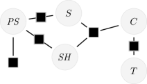
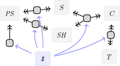
Figure 4: Conversion of the PDG in Example 2 to a factor graph according to Definition 4.2 (left), and from that factor graph back to a PDG by Definition 4.3 (right). In the latter, for each $J$ we introduce a new variable $X_{J}$ (displayed as a smaller darker rectangle), whose values are joint settings of the variables connected it, and also an edge $1\to X_{J}$ (shown in blue), to which we associate the unconditional distribution given by normalizing $\phi_{J}$.

PDGs are directed graphs, while factors graphs are undirected. The map from PDGs to factor graphs thus loses some important structure. As shown in Figure 4, this mapping can change the graphical structure significantly. Nevertheless,

Theorem 4.2 (name=,restate=thm:fg-is-pdg,label=thm:fg-is-pdg).

$\Pr_{\Phi}=[\mspace{-3.5mu}[{\mathbdcal{N}}_{\Phi}]\mspace{-3.5mu}]_{1}^{*}\;$ for all factor graphs $\Phi$.

Theorem 4.3 (name=,restate=thm:pdg-is-fg,label=thm:pdg-is-fg).

$[\mspace{-3.5mu}[\mathbdcal{N}]\mspace{-3.5mu}]_{1}^{*}=\Pr_{\Phi_{{\mathbdcal{N}}}}\;$ for all unweighted PDGs $\mathbdcal{N}$.

The correspondence hinges on the fact that we take $\gamma=1$, so that $\mathit{Inc}$ and $\mathit{IDef}_{\!}$ are weighted equally. Because the user of a PDG gets to choose $\gamma$, the fact that the translation from factor graphs to PDGs preserves semantics only for $\gamma=1$ poses no problem. Conversely, the fact that the reverse correspondence requires $\gamma=1$ suggests that factor graphs are less flexible than PDGs.

What about weighted PDGs $(\mathcal{G},\mathbf{p},\beta)$ where $\beta\neq{\bf 1}$? There is also a standard notion of weighted factor graph, but as long as we stick with our convention of taking $\alpha={\bf 1}$, we cannot relate them to weighted PDGs. As we are about to see, once we drop this convention, we can do much more.

4.3 Factored Exponential Families

A weighted factor graph (WFG) $\Psi$ is a pair $(\Phi,\theta)$ consisting of a factor graph $\Phi$ together with a vector of non-negative weights $\{\theta_{J}\}_{J\in\mathcal{J}}$. $\Psi$ specifies a canonical scoring function

$$\mathit{G\mkern-4.0muF\mkern-4.5muE}_{\Psi}(\mu):=\!\operatorname*{\mathbb{E}}_{\vec{x}\sim\mu}\left[\sum_{J\in\cal J}\theta_{J}\log\frac{1}{\phi_{J}(\vec{x}_{J})}\right]-\operatorname{\mathrm{H}}(\mu),$$ (4)

called the variational Gibbs free energy (Mezard and Montanari 2009). $\mathit{G\mkern-4.0muF\mkern-4.5muE}_{\Psi}$ is uniquely minimized by the distribution ${\Pr}_{\Psi}(\vec{x})=\frac{1}{Z_{\Psi}}\prod_{J\in\cal J}\phi_{J}(\vec{x}_{J})^{\theta_{J}}$, which matches the unweighted case when every $\theta_{J}=1$. The mapping $\theta\mapsto\Pr_{(\Phi,\theta)}$ is known as $\Phi$’s exponential family and is a central tool in the analysis and development of many algorithms for graphical models (Wainwright, Jordan et al. 2008).

PDGs can in fact capture the full exponential family of a factor graph, but only by allowing values of $\alpha$ other than ${\bf 1}$. In this case, the only definition that requires alteration is $\mathit{IDef}_{\!}$, which now depends on the weighted multigraph $(\mathcal{G}^{\mathbdcal{M}},\alpha^{\mathbdcal{M}})$, and is given by

$$\mathit{IDef}_{\!\mathbdcal{M}}(\mu):=\sum_{X\!\overset{\smash{\mskip-5.0mu\raisebox{-1.0pt}{$\scriptscriptstyle L$}}}{\rightarrow}\!Y\in\mathcal{E}}\alpha_{L}\operatorname{\mathrm{H}}_{\mu}(Y\mid X)-\operatorname{\mathrm{H}}(\mu).$$ (5)

Thus, the conditional entropy $\operatorname{\mathrm{H}}_{\mu}(Y\mid X)$ associated with the edge $X\!\overset{\smash{\mskip-5.0mu\raisebox{-1.0pt}{$\scriptscriptstyle L$}}}{\rightarrow}\!Y$ is multiplied by the weight $\alpha_{L}$ of that edge.

One key benefit of using $\alpha$ is that we can capture arbitrary WFGs, not just ones with a constant weight vector. All we have to do is to ensure that in our translation from factor graphs to PDGs, the ratio $\alpha_{L}/\beta_{L}$ is a constant. (Of course, if we allow arbitrary weights, we cannot hope to do this if $\alpha_{L}=1$ for all edges $L$.) We therefore define a family of translations, parameterized by the ratio of $\alpha_{L}$ to $\beta_{L}$.

Definition 4.4 (WFG to PDG).

Given a WFG $\Psi=(\Phi,\theta)$, and postive number $k$, we define the corresponding PDG ${\mathbdcal{M}}_{\Psi,k}=({\mathbdcal{N}}_{\Phi},\alpha_{\theta},\beta_{\theta})$ by taking $\beta_{J}=k\theta_{J}$ and $\alpha_{J}=\theta_{J}$ for the edge $\mathrlap{\mathit{1}}\mspace{2.3mu}\mathit{1}\rightarrow X_{J}$, and taking $\beta_{L}=k$ and $\alpha_{L}=1$ for the projections $X_{J}\!\rightarrow\mathrel{\mspace{-15.0mu}}\rightarrow\!X_{j}$.

We now extend Definitions 4.2 and 4.3 to (weighted) PDGs and WFGs. In translating a PDG to a WFG, there will necessarily be some loss of information: PDGs have two sets, while WFGs have only have one. Here we throw out $\alpha$ and keep $\beta$, though in its role here as a left inverse of Definition 4.4, either choice would suffice.

Definition 4.5 (PDG to WFG).

Given a (weighted) PDG $\mathbdcal{M}=(\mathbdcal{N},\beta)$, we take its corresponding WFG to be $\Psi_{{\mathbdcal{M}}}:=(\Phi_{{\mathbdcal{N}}},\beta)$; that is, $\theta_{L}:=\beta_{L}$ for all edges $L$.

We now show that we can capture the entire exponential family of a factor graph, and even its associated free energy, but only for $\gamma$ equal to the constant $k$ used in the translation.

Theorem 4.4.

For all WFGs $\Psi=(\Phi,\theta)$ and all $\gamma>0$, we have that $\mathit{G\mkern-4.0muF\mkern-4.5muE}_{\Psi}=\nicefrac{{1}}{{\gamma}}[\mspace{-3.5mu}[{\mathbdcal{M}}_{\Psi,\gamma}]\mspace{-3.5mu}]_{\gamma}+C$ for some constant $C$, so $\Pr_{\Psi}$ is the unique element of $[\mspace{-3.5mu}[{\mathbdcal{M}}_{\Psi,\gamma}]\mspace{-3.5mu}]_{\gamma}^{*}$.

In particular, for $k\!=\!1$, so that $\theta$ is used for both the functions $\alpha$ and $\beta$ of the resulting PDG, Theorem 4.4 strictly generalizes LABEL:thm:fg-is-pdg.

Corollary 4.4.1.

For all weighted factor graphs $(\Phi,\theta)$, we have that $\Pr_{(\Phi,\theta)}=[\mspace{-3.5mu}[({\mathbdcal{N}}_{\Phi},\theta,\theta)]\mspace{-3.5mu}]_{1}^{*}$

Conversely, as long as the ratio of $\alpha_{L}$ to $\beta_{L}$ is constant, the reverse translation also preserves semantics.

Theorem 4.5 (name=,restate=thm:pdg-is-wfg,label=thm:pdg-is-wfg).

For all unweighted PDGs $\mathbdcal{N}$ and non-negative vectors $\mathbf{v}$ over $\mathcal{E}^{\mathbdcal{N}}$, and all $\gamma>0$, we have that $[\mspace{-3.5mu}[(\mathbdcal{N},\mathbf{v},\gamma\mathbf{v})]\mspace{-3.5mu}]_{\gamma}=\gamma\,\mathit{G\mkern-4.0muF\mkern-4.5muE}_{(\Phi_{\mathbdcal{N}},\mathbf{v})}$; consequently, $[\mspace{-3.5mu}[(\mathbdcal{N},\mathbf{v},\gamma\mathbf{v})]\mspace{-3.5mu}]_{\gamma}^{*}=\{\Pr_{(\Phi_{\mathbdcal{N}},\mathbf{v})}\}$.

The key step in proving Theorems 4.4 and LABEL:thm:pdg-is-wfg (and in the proofs of a number of other results) involves rewriting $[\mspace{-3.5mu}[\mathbdcal{M}]\mspace{-3.5mu}]_{\gamma}$ as follows:

Proposition 4.6 (restate=prop:nice-score,label=prop:nice-score).

Letting $x^{\mathbf{w}}$ and $y^{\mathbf{w}}$ denote the values of $X$ and $Y$, respectively, in $\mathbf{w}\in\mathcal{V}(\mathbdcal{M})$, we have

$$\begin{split}[\mspace{-3.5mu}[\mathbdcal{M}]\mspace{-3.5mu}](\mu)=\operatorname*{\mathbb{E}}_{\mathbf{w}\sim\mu}\!\Bigg{\{}\sum_{X\xrightarrow{\!\!L}Y}\bigg{[}\,\color[rgb]{.5,.5,.5}\overbrace{\color[rgb]{0,0,0}\!\beta_{L}\log\frac{1}{\mathbf{p}_{\!{}_{L}\!}(y^{\mathbf{w}}|x^{\mathbf{w}})}}^{\color[rgb]{.5,.5,.5}\smash{\mathclap{\text{log likelihood / cross entropy}}}}+\qquad\\[-6.99997pt] \color[rgb]{.5,.5,.5}\underbrace{\color[rgb]{0,0,0}({\alpha_{L}}\gamma-\beta_{L})\log\frac{1}{\mu(y^{\mathbf{w}}|x^{\mathbf{w}})}}_{\color[rgb]{.5,.5,.5}\smash{\mathclap{\text{local regularization (if $\beta_{L}>\alpha_{L}\gamma$)}}}}\bigg{]}-\underbrace{\color[rgb]{0,0,0}\gamma\log\frac{1}{\mu(\mathbf{w})}}_{\color[rgb]{.5,.5,.5}\smash{\mathclap{\text{global regularization}}}}\color[rgb]{0,0,0}\Bigg{\}}.\end{split}$$ (6)

For a fixed $\gamma$, the first and last terms of (6) are equal to a scaled version of the free energy, $\gamma\mathit{G\mkern-4.0muF\mkern-4.5muE}_{\Phi}$, if we set $\phi_{J}:=\mathbf{p}_{\!{}_{L}\!}$ and $\theta_{J}:=\nicefrac{{\beta_{L}}}{{\gamma}}$. If, in addition, $\beta_{L}={\alpha_{L}}\gamma$ for all edges $L$, then the local regularization term disappears, giving us the desired correspondence.

Equation 6 also makes it clear that taking $\beta_{L}={\alpha_{L}}\gamma$ for all edges $L$ is essentially necessary to get LABEL:thm:pdg-is-fg and LABEL:thm:fg-is-pdg. Of course, fixed $\gamma$ precludes taking the limit as $\gamma$ goes to 0, so LABEL:prop:consist does apply. This is reflected in some strange behavior in factor graphs trying to capture the same phenomena as PDGs, as the following example shows.

Example 5.

Consider the PDG $\mathbdcal{M}$ containing just $X$ and $1$, and two edges $p,q:1\to X$. (Recall that such a PDG can arise if we get different information about the probability of $X$ from two different sources; this is a situation we certainly want to be able to capture!) Consider the simplest situation, where $p$ and $q$ are both associated with the same distribution on $X$; further suppose that the agent is certain about the distribution, so $\beta_{p}=\beta_{q}=1$. For definiteness, suppose that $\mathcal{V}(X)=\{x_{1},x_{2}\}$, and that the distribution associated with both edges is $\mu_{.7}$, which ascribes probability $.7$ to $x_{1}$. Then, as we would hope $[\mspace{-3.5mu}[\mathbdcal{M}]\mspace{-3.5mu}]^{*}=\{\mu_{.7}\}$; after all, both sources agree on the information. However, it can be shown that $\Pr_{\Psi_{{\mathbdcal{M}}}}=\mu_{.85}$, so $[\mspace{-3.5mu}[\mathbdcal{M}]\mspace{-3.5mu}]_{1}^{*}=\{\mu_{.85}\}$.

Although both $\theta$ and $\beta$ are measures of confidence, the way that the Gibbs free energy varies with $\theta$ is quite different from the way that the score of a PDG varies with $\beta$. The scoring function that we use for PDGs can be viewed as extending ${\mathit{G\mkern-4.0muF\mkern-4.5muE}}_{\Phi,\theta}$ by including the local regularization term. As $\gamma$ approaches zero, the importance of the global regularization terms decreases relative to that of the local regularization term, so the PDG scoring function becomes quite different from Gibbs free energy.

5 Discussion

We have introduced PDGs, a powerful tool for representing probabilistic information. They have a number of advantages over other probablisitic graphical models.

• They allow us to capture inconsistency, including conflicting information from multiple sources with varying degrees of reliability.

• They are much more modular than other representations; for example, we can combine information from two sources by simply taking the union of two PDGs, and it is easy to add new information (edges) and features (nodes) without affecting previously-received information.

• They allow for a clean separation between quantitiatve information (the cpds and weights $\beta$) and more qualitative information contained by the graph structure (and the weights $\alpha$); this is captured by the terms $\mathit{Inc}$ and $\mathit{IDef}_{\!}$ in our scoring function.

• PDGs have (several) natural semantics; one of them allows us to pick out a unique distribution. Using this distrbution, PDGs can capture BNs and factor graphs. In the latter case, a simple parameter shift in the corresponding PDG eliminates arguably problematic behavior of a factor graph.

We have only scratched the surface of what can be done with PDGs here. Two major issues that need to be tackled are inference and dynamics. How should we query a PDG for probabilistic information? How should we modify a PDG in light of new information or to make it more consistent? These issues turn out to be closely related. Due to space limitations, we just briefly give some intuitions and examples here.

Suppose that we want to compute the probability of $Y$ given $X$ in a PDG $\mathbdcal{M}$. For a cpd $p(Y|X)$, let $\mathbdcal{M}^{+p}$ be the PDG obtained by associating $p$ with a new edge in $\mathbdcal{M}$ from $X$ to $Y$, with $\alpha_{p}\!=\!0$. We judge the quality of a candidate answer $p$ by the best possible score that $\mathbdcal{M}^{+p}$ gives to any distribution (which we call the degree of inconsistency of $\mathbdcal{M}^{+p}$). It can be shown that the deegree of inconsistency is minimized by $[\mspace{-3.5mu}[\mathbdcal{M}]\mspace{-3.5mu}]^{*}(Y\!\mid\!X)$. Since the degree of inconsistency of $\mathbdcal{M}^{+p}$ is smooth and strongly convex as a function of $p$, we can compute its optimum values by standard gradient methods. This approach is inefficient as written (since it involves computing the full joint distribution $[\mspace{-3.5mu}[{\mathbdcal{M}}^{+p}]\mspace{-3.5mu}]^{*}$), but we believe that standard approximation techniques will allow us to draw inferences efficiently.

To take another example, conditioning can be understood in terms of resolving inconsistencies in a PDG. To condition on an observation $Y\!=\!y$, given a situation described by a PDG $\mathbdcal{M}$, we can add an edge from $\mathrlap{\mathit{1}}\mspace{2.3mu}\mathit{1}$ to $Y$ in $\mathbdcal{M}$, annoted with the cpd that gives probability 1 to $y$, to get the (possibly inconsistent) PDG ${\mathbdcal{M}}^{+(\!Y\!=y)}$. The distribution $[\mspace{-3.5mu}[{\mathbdcal{M}}^{+(\!Y\!=y)}]\mspace{-3.5mu}]^{*}$ turns out to be the result of conditioning $[\mspace{-3.5mu}[\mathbdcal{M}]\mspace{-3.5mu}]^{*}$ on $Y\!=\!y$. This account of conditioning generalizes without modification to give Jeffrey’s Rule (Jeffrey 1968), a more general approach to belief updating.

Issues of updating and inconsistency also arise in variational inference. A variational autoencoder (Kingma and Welling 2013), for instance, is essentially three cpds: a prior $p(Z)$, a decoder $p(X\!\mid\!Z)$, and an encoder $q(Z\!\mid\!X)$. Because two cpds target $Z$ (and the cpds are inconsistent until fully trained), this situation can be represented by PDGs but not by other graphical models. We hope to report further on the deep connection between inference, updating, and the resolution of inconsistency in PDGs in future work.

Ethics Statement

Because PDGs are a recent theoretical development, there is a lot of guesswork in evaluating the impact. Here are two views of opposite polarity.

5.1 Positive Impacts

One can imagine many applications of enabling simple and coherent aggregation of (possibly inconsistent) information. In particular we can imagine using PDGs to build and interpret a communal and global database of statistical models, in a way that may not only enable more accurate predictions, but also highlights conflicts between information.

This could have many benefits. Suppose, for instance, that two researchers train models, but use datasets with different racial makeups. Rather than trying to get an uninterpretable model to “get it right” the first time, we could simply highlight any such clashes and flag them for review.

Rather than trying to ensure fairness by design, which is both tricky and costly, we envision an alternative: simply aggregate (conflicting) statistically optimal results, and allow existing social structure to resolve conflicts, rather than sending researchers to fiddle with loss functions until they look fair.

5.2 Negative Impacts

We can also imagine less rosy outcomes. To the extent that PDGs can model and reason with inconsistency, if we adopt the attitude that a PDG need not wait until it is consistent to be used, it is not hard to imagine a world where a PDG gives biased and poorly-thought out conclusions. It is clear that PDGs need a great deal more vetting before they can be used for such important purposes as aggregating the world’s statistical knowledge.

PDGs are powerful statistical models, but are by necessity semantically more complicated than many existing methods. This will likely restrict their accessibility. To mitigate this, we commit to making sure our work is widely accessible to researchers of different backgrounds.

Appendix A Proofs

For brevity, we use the standard notation and write $\mu(x,y)$ instead of $\mu(X\!=\!x,Y\!=\!y)$, $\mu(x\mid y)$ instead of $\mu(X\!=\!x\mid Y\!=\!y)$, and so forth.

A.1 Properties of Scoring Semantics

In this section, we prove the properties of scoring functions that we mentioned in the main text, Propositions LABEL:prop:sd-is-zeroset, LABEL:prop:sem3, and LABEL:prop:consist. We repeat the statements for the reader’s convenience.

LABEL:thmt@@prop:sd-is-zeroset. $[\mspace{-3.5mu}[\mathbdcal{M}]\mspace{-3.5mu}]_{\text{sd}}\!=\{\mu:[\mspace{-3.5mu}[\mathbdcal{M}]\mspace{-3.5mu}]_{0}(\mu)\!=\!0\}$ for all $\mathbdcal{M}$.

Proof.

By taking $\gamma=0$, the score is just $\mathit{Inc}$. By definition, a distribution $\mu\in[\mspace{-3.5mu}[\mathbdcal{M}]\mspace{-3.5mu}]_{\text{sd}}$ satisfies all the constraints, so $\mu(Y=\cdot\mid X=x)=\mathbf{p}_{\!{}_{L}\!}(x)$ for all edges $X\rightarrow Y\in\mathcal{E}^{\mathbdcal{M}}$ and $x$ with $\mu(X=x)>0$. By Gibbs inequality (MacKay 2003), $I\mkern-8.0muD(\mu(Y|x)\;\|\;\mathbf{p}_{\!{}_{L}\!}(x))=0$. Since this is true for all edges, we must have $\mathit{Inc}_{\mathbdcal{M}}(\mu)=0$. Conversely, if $\mu\notin[\mspace{-3.5mu}[\mathbdcal{M}]\mspace{-3.5mu}]_{\text{sd}}$, then it fails to marginalize to the cpd $\mathbf{p}_{\!{}_{L}\!}$ on some edge $L$, and so again by Gibbs inequality, $I\mkern-8.0muD(\mu(Y|x)\;\|\;\mathbf{p}_{\!{}_{L}\!}(x))>0$. As relative entropy is non-negative, the sum of these terms over all edges must be positive as well, and so $\mathit{Inc}_{\mathbdcal{M}}(\mu)\neq 0$. ∎

Before proving the remaining results, we prove a lemma that will be useful in other contexts as well.

Lemma A.1.

$\mathit{Inc}_{\mathbdcal{M}}(\mu)$ is a convex function of $\mu$.

Proof.

It is well known that $I\mkern-8.0muD$ is convex (Cover and Thomas 1991, Theorem 2.7.2), in the sense that

$$I\mkern-8.0muD(\lambda q_{1}+(1-\lambda)q_{2}\;\|\;\lambda p_{1}+(1-\lambda)p_{2})\leq\lambda I\mkern-8.0muD(q_{1}\;\|\;p_{1})+(1-\lambda)I\mkern-8.0muD(q_{2}\;\|\;p_{2}).$$

Given an edge $L\in\mathcal{E}$ from $A$ to $B$ and $a\in\mathcal{V}(A)$, and setting $q_{1}=q_{2}=\mathbf{p}_{\!{}_{L}\!}(a)$, we get that

$$I\mkern-8.0muD(\mathbf{p}_{\!{}_{L}\!}(a)\ ||\ \lambda p_{1}+(1-\lambda)p_{2})\leq\lambda I\mkern-8.0muD(\mathbf{p}_{\!{}_{L}\!}(a)\ ||\ p_{1})+(1-\lambda)I\mkern-8.0muD(\mathbf{p}_{\!{}_{L}\!}(a)\ ||\ p_{2}).$$

Since this is true for every $a$ and edge, we can take a weighted sum of these inequalities for each $a$ weighted by $p(A=a)$; thus,

$$\operatorname*{\mathbb{E}}_{a\sim p_{A}}I\mkern-8.0muD(\mathbf{p}_{\!{}_{L}\!}(a)\;\|\;\lambda p_{1}+(1-\lambda)p_{2}) \leq\operatorname*{\mathbb{E}}_{a\sim p_{A}}\lambda I\mkern-8.0muD(\mathbf{p}_{\!{}_{L}\!}(a)\;\|\;p_{1})+(1-\lambda)I\mkern-8.0muD(\mathbf{p}_{\!{}_{L}\!}(a)\;\|\;p_{2}).$$

Taking a sum over all edges, we get that

$$\sum_{(A,B)\in\mathcal{E}}\mskip-10.0mu\operatorname*{\mathbb{E}}_{a\sim p_{A}}I\mkern-8.0muD(\mathbf{p}_{\!{}_{L}\!}(a)\;\|\;\lambda p_{1}+(1-\lambda)p_{2}) \leq\sum_{(A,B)\in\mathcal{E}}\mskip-10.0mu\operatorname*{\mathbb{E}}_{a\sim p_{A}}\lambda I\mkern-8.0muD(\mathbf{p}_{\!{}_{L}\!}(a)\;\|\;p_{1})+(1-\lambda)I\mkern-8.0muD(\mathbf{p}_{\!{}_{L}\!}(a)\;\|\;p_{2}).$$

It follows that

$$\mathit{Inc}_{\mathbdcal{M}}(\lambda p_{1})+(1-\lambda)p_{2}) \leq\lambda\mathit{Inc}_{\mathbdcal{M}}(p_{1})+(1-\lambda)\mathit{Inc}_{\mathbdcal{M}}(p_{2}).$$

Therefore, $\mathit{Inc}_{\mathbdcal{M}}(\mu)$ is a convex function of $\mu$. ∎

The next proposition gives us a useful representation of $[\mspace{-3.5mu}[M]\mspace{-3.5mu}]_{\gamma}$.

LABEL:thmt@@prop:nice-score. Letting $x^{\mathbf{w}}$ and $y^{\mathbf{w}}$ denote the values of $X$ and $Y$, respectively, in $\mathbf{w}\in\mathcal{V}(\mathbdcal{M})$, we have

$$\begin{split}[\mspace{-3.5mu}[\mathbdcal{M}]\mspace{-3.5mu}](\mu)=\operatorname*{\mathbb{E}}_{\mathbf{w}\sim\mu}\!\Bigg{\{}\sum_{X\xrightarrow{\!\!L}Y}\bigg{[}\,\!\beta_{L}\log\frac{1}{\mathbf{p}_{\!{}_{L}\!}(y^{\mathbf{w}}|x^{\mathbf{w}})}+({\alpha_{L}}\gamma-\beta_{L})\log\frac{1}{\mu(y^{\mathbf{w}}|x^{\mathbf{w}})}\bigg{]}-\gamma\log\frac{1}{\mu(\mathbf{w})}\Bigg{\}}.\end{split}$$

Proof.

We use the more general formulation of $\mathit{IDef}_{\!}$ given in Section 4.3, in which each edge $L$’s conditional information is weighted by $\alpha_{L}$.

$$[\mspace{-3.5mu}[\mathbdcal{M}]\mspace{-3.5mu}]_{\gamma}(\mu) :=\mathit{Inc}_{\mathbdcal{M}}(\mu)+\gamma\mathit{IDef}_{\!\mathbdcal{M}}(\mu)$$

$$=\left[\sum_{X\!\overset{\smash{\mskip-5.0mu\raisebox{-1.0pt}{$\scriptscriptstyle L$}}}{\rightarrow}\!Y}\beta_{L}\operatorname*{\mathbb{E}}_{x\sim\mu_{X}}I\mkern-8.0muD\Big{(}\mu(Y|X\!=\!x)\;\Big{\|}\;\mathbf{p}_{\!{}_{L}\!}(x)\Big{)}\right]+\gamma\left[\sum_{X\!\overset{\smash{\mskip-5.0mu\raisebox{-1.0pt}{$\scriptscriptstyle L$}}}{\rightarrow}\!Y}\alpha_{L}\operatorname{\mathrm{H}}_{\mu}(Y\mid X)~{}-\operatorname{\mathrm{H}}(\mu)\right]$$

$$=\sum_{X\!\overset{\smash{\mskip-5.0mu\raisebox{-1.0pt}{$\scriptscriptstyle L$}}}{\rightarrow}\!Y}\operatorname*{\mathbb{E}}_{x\sim\mu_{\!{}_{X}}}\left[\beta_{L}\;I\mkern-8.0muD\Big{(}\mu(Y\mid x)\;\Big{\|}\;\mathbf{p}_{\!{}_{L}\!}(Y\mid x)\Big{)}+\gamma\;\alpha_{L}\operatorname{\mathrm{H}}(Y\mid X\!=\!x)\right]-\gamma\operatorname{\mathrm{H}}(\mu)$$

$$=\sum_{X\!\overset{\smash{\mskip-5.0mu\raisebox{-1.0pt}{$\scriptscriptstyle L$}}}{\rightarrow}\!Y}\operatorname*{\mathbb{E}}_{x\sim\mu_{\!{}_{X}}}\left[\beta_{L}\;\left(\sum_{y\in\mathcal{V}(Y)}\mu(y\mid x)\log\frac{\mu(y\mid x)}{\mathbf{p}_{\!{}_{L}\!}(y\mid x)}\right)+\alpha_{L}\gamma\;\left(\sum_{y\in\mathcal{V}(Y)}\mu(y\mid x)\log\frac{1}{\mu(y\mid x)}\right)\right]-\gamma\operatorname{\mathrm{H}}(\mu)$$

$$=\sum_{X\!\overset{\smash{\mskip-5.0mu\raisebox{-1.0pt}{$\scriptscriptstyle L$}}}{\rightarrow}\!Y}\operatorname*{\mathbb{E}}_{x\sim\mu_{\!{}_{X}}}\left[\sum_{y\in\mathcal{V}(Y)}\mu(y\mid x)\left(\beta_{L}\;\log\frac{\mu(y\mid x)}{\mathbf{p}_{\!{}_{L}\!}(y\mid x)}+\alpha_{L}\gamma\;\log\frac{1}{\mu(y\mid x)}\right)\right]-\gamma\operatorname{\mathrm{H}}(\mu)$$

$$=\sum_{X\!\overset{\smash{\mskip-5.0mu\raisebox{-1.0pt}{$\scriptscriptstyle L$}}}{\rightarrow}\!Y}\operatorname*{\mathbb{E}}_{x\sim\mu_{\!{}_{X}}}\left[\operatorname*{\mathbb{E}}_{y\sim\mu(Y\mid X=x)}\left(\beta_{L}\;\log\frac{\mu(y\mid x)}{\mathbf{p}_{\!{}_{L}\!}(y\mid x)}+\alpha_{L}\gamma\;\log\frac{1}{\mu(y\mid x)}\right)\right]-\gamma\sum_{\mathbf{w}\in\mathcal{V}(\mathbdcal{M})}\mu(\mathbf{w})\log\frac{1}{\mu(\mathbf{w})}$$

$$=\sum_{X\!\overset{\smash{\mskip-5.0mu\raisebox{-1.0pt}{$\scriptscriptstyle L$}}}{\rightarrow}\!Y}\operatorname*{\mathbb{E}}_{x,y\sim\mu_{\!{}_{XY}}}\left[\beta_{L}\;\log\frac{\mu(y\mid x)}{\mathbf{p}_{\!{}_{L}\!}(y\mid x)}+\alpha_{L}\gamma\;\log\frac{1}{\mu(y\mid x)}\right]-\gamma\operatorname*{\mathbb{E}}_{\mathbf{w}\sim\mu}\left[\log\frac{1}{\mu(\mathbf{w})}\right]$$

$$=\operatorname*{\mathbb{E}}_{\mathbf{w}\sim\mu}\Bigg{\{}\sum_{X\xrightarrow{\!\!L}Y}\left[\beta_{L}\log\frac{1}{\mathbf{p}_{\!{}_{L}\!}(y\mid x)}-\beta_{L}\log\frac{1}{\mu(y\mid x)}+\alpha_{L}\gamma\log\frac{1}{\mu(y\mid x)}\right]\Bigg{\}}-\gamma\operatorname*{\mathbb{E}}_{\mathbf{w}\sim\mu}\left[\log\frac{1}{\mu(\mathbf{w})}\right]$$

$$=\operatorname*{\mathbb{E}}_{\mathbf{w}\sim\mu}\Bigg{\{}\sum_{X\xrightarrow{\!\!L}Y}\left[\beta_{L}\log\frac{1}{\mathbf{p}_{\!{}_{L}\!}(y\mid x)}+(\alpha_{L}\gamma-\beta_{L})\log\frac{1}{\mu(y\mid x)}\right]-\gamma\log\frac{1}{\mu(\mathbf{w})}\Bigg{\}}.$$

∎

We can now prove Proposition LABEL:prop:sem3.

LABEL:thmt@@prop:sem3. If $\mathbdcal{M}$ is a PDG and $0<\gamma\leq\min_{L}\nicefrac{{\beta_{L}^{\mathbdcal{M}}}}{{\alpha_{L}^{\mathbdcal{M}}}}$, then $[\mspace{-3.5mu}[\mathbdcal{M}]\mspace{-3.5mu}]_{\gamma}^{*}$ is a singleton.

Proof.

It suffices to show that $[\mspace{-3.5mu}[\mathbdcal{M}]\mspace{-3.5mu}]_{\gamma}$ is a strictly convex function of $\mu$, since every strictly convex function has a unique minimum. Note that

$$[\mspace{-3.5mu}[M]\mspace{-3.5mu}]_{\gamma}(\mu) =\operatorname*{\mathbb{E}}_{\mathbf{w}\sim\mu}\Bigg{\{}\sum_{X\xrightarrow{\!\!L}Y}\left[\beta_{L}\log\frac{1}{\mathbf{p}_{\!{}_{L}\!}(y\mid x)}+({\alpha_{L}}\gamma-\beta_{L})\log\frac{1}{\mu(y\mid x)}\right]-\gamma\log\frac{1}{\mu(\mathbf{w})}\Bigg{\}}$$

$$=\operatorname*{\mathbb{E}}_{\mathbf{w}\sim\mu}\Bigg{\{}\sum_{X\xrightarrow{\!\!L}Y}\left[\gamma{\alpha_{L}}\log\frac{1}{\mathbf{p}_{\!{}_{L}\!}(y\mid x)}+(\beta_{L}-{\alpha_{L}}\gamma)\log\frac{1}{\mathbf{p}_{\!{}_{L}\!}(y\mid x)}-(\beta_{L}-{\alpha_{L}}\gamma)\log\frac{1}{\mu(y\mid x)}\right]-\gamma\log\frac{1}{\mu(\mathbf{w})}\Bigg{\}}$$

$$=\operatorname*{\mathbb{E}}_{\mathbf{w}\sim\mu}\Bigg{\{}\sum_{X\xrightarrow{\!\!L}Y}\left[\gamma{\alpha_{L}}\log\frac{1}{\mathbf{p}_{\!{}_{L}\!}(y\mid x)}+(\beta_{L}-{\alpha_{L}}\gamma)\log\frac{\mu(y\mid x)}{\mathbf{p}_{\!{}_{L}\!}(y\mid x)}\right]-\gamma\log\frac{1}{\mu(\mathbf{w})}\Bigg{\}}$$

$$=\sum_{X\xrightarrow{\!\!L}Y}\left[\gamma{\alpha_{L}}\operatorname*{\mathbb{E}}_{x,y\sim\mu_{\!{}_{XY}}}\left[\log\frac{1}{\mathbf{p}_{\!{}_{L}\!}(y\mid x)}\right]+(\beta_{L}-{\alpha_{L}}\gamma)\operatorname*{\mathbb{E}}_{x\sim\mu_{X}}I\mkern-8.0muD\Big{(}\mu(Y\mid x)\;\Big{\|}\;\mathbf{p}_{\!{}_{L}\!}(x)\Big{)}\right]-\gamma\operatorname{\mathrm{H}}(\mu).$$

The first term, $\operatorname*{\mathbb{E}}_{x,y\sim\mu_{\!{}_{XY}}}\left[-\log{\mathbf{p}_{\!{}_{L}\!}(y\mid x)}\right]$ is linear in $\mu$, as $\mathbf{p}_{\!{}_{L}\!}(y\mid x)$ does not depend on $\mu$. As for the second term, it is well-known that KL divergence is convex, in the sense that

$$I\mkern-8.0muD(\lambda q_{1}+(1-\lambda)q_{2}\;\|\;\lambda p_{1}+(1-\lambda)p_{2})\leq\lambda I\mkern-8.0muD(q_{1}\;\|\;p_{1})+(1-\lambda)I\mkern-8.0muD(q_{2}\;\|\;p_{2}).$$

Therefore, for a distribution on $Y$, setting $p_{1}=p_{2}=\mathbf{p}_{\!{}_{L}\!}(x)$, for all conditional marginals $\mu_{1}(Y\mid X=x)$ and $\mu_{2}(Y\mid X=x)$,

$$I\mkern-8.0muD(\lambda\mu_{1}(Y\mid x)+(1-\lambda)\mu_{2}(Y\mid x)\;\|\;\mathbf{p}_{\!{}_{L}\!}(x))\leq\lambda I\mkern-8.0muD(\mu_{1}(Y\mid x)\;\|\;\mathbf{p}_{\!{}_{L}\!}(x))+(1-\lambda)I\mkern-8.0muD(\mu_{2}(Y\mid x)\;\|\;\mathbf{p}_{\!{}_{L}\!}(x)).$$

So $I\mkern-8.0muD\left(\mu(Y\mid x)\;\middle\|\;\mathbf{p}_{\!{}_{L}\!}(x)\right)$ is convex. As convex combinations of convex functions are convex, the second term, $\operatorname*{\mathbb{E}}_{x\sim\mu_{X}}I\mkern-8.0muD\left(\mu(Y\mid x)\;\middle\|\;\mathbf{p}_{\!{}_{L}\!}(x)\right)$, is convex. Finally, negative entropy is well known to be strictly convex.

Any non-negative linear combinations of the three terms is convex, and if this combination applies a positive coefficient to the (strictly convex) negative entropy, it must be strictly convex. Therefore, as long as $\beta_{L}\geq\gamma$ for all edges $L\in\mathcal{E}^{\mathbdcal{M}}$, $[\mspace{-3.5mu}[\mathbdcal{M}]\mspace{-3.5mu}]_{\gamma}$ is strictly convex. The result follows. ∎

We next prove LABEL:prop:limit-uniq. The first step is provided by the following lemma.

Lemma A.2.

$\lim\limits_{\gamma\to 0}[\mspace{-3.5mu}[\mathbdcal{M}]\mspace{-3.5mu}]_{\gamma}^{*}\subseteq[\mspace{-3.5mu}[\mathbdcal{M}]\mspace{-3.5mu}]_{0}^{*}$.

Proof.

Since $\mathit{IDef}_{\!\mathbdcal{M}}$ is a finite weighted sum of entropies and conditional entropies over the variables $\mathcal{N}^{\mathbdcal{M}}$, which have finite support, it is bounded. Thus, there exist bounds $k$ and $K$ depending only on $\mathcal{N}^{\mathbdcal{M}}$ and $\mathcal{V}^{\mathbdcal{M}}$, such that $k\leq\mathit{IDef}_{\!\mathbdcal{M}}(\mu)\leq K$ for all $\mu$. Since $[\mspace{-3.5mu}[\mathbdcal{M}]\mspace{-3.5mu}]_{\gamma}=\mathit{Inc}_{\mathbdcal{M}}+\gamma\mathit{IDef}_{\!\mathbdcal{M}}$, it follows that, for all $\mu\in\mathcal{V}(\mathbdcal{M})$, we have

$$\mathit{Inc}_{\mathbdcal{M}}(\mu)+\gamma k\leq~{}[\mspace{-3.5mu}[\mathbdcal{M}]\mspace{-3.5mu}]_{\gamma}(\mu)\leq~{}\mathit{Inc}_{\mathbdcal{M}}(\mu)+\gamma K.$$

For a fixed $\gamma$, since this inequality holds for all $\mu$, and both $\mathit{Inc}$ and $\mathit{IDef}_{\!}$ are bounded below, it must be the case that

$$\min_{\mu\in\Delta\mathcal{V}(\mathbdcal{M})}\Big{[}\mathit{Inc}_{\mathbdcal{M}}(\mu)+\gamma k\Big{]}~{}\leq~{}\min_{\mu\in\Delta\mathcal{V}(\mathbdcal{M})}[\mspace{-3.5mu}[\mathbdcal{M}]\mspace{-3.5mu}]_{\gamma}(\mu)~{}\leq~{}\min_{\mu\in\Delta\mathcal{V}(\mathbdcal{M})}\Big{[}\mathit{Inc}_{\mathbdcal{M}}(\mu)+\gamma K\Big{]},$$

even though the distributions that minimize each expression will in general be different. Let $\mathit{Inc}(\mathbdcal{M})=\min_{\mu}\mathit{Inc}_{\mathbdcal{M}}(\mu)$. Since $\Delta\mathcal{V}(\mathbdcal{M})$ is compact, the minimum of the middle term is achieved. Therefore, for $\mu_{\gamma}\in[\mspace{-3.5mu}[\mathbdcal{M}]\mspace{-3.5mu}]^{*}_{\gamma}(\mu)$ that minimizes it, we have

$$\mathit{Inc}(\mathbdcal{M})+\gamma k\leq[\mspace{-3.5mu}[\mathbdcal{M}]\mspace{-3.5mu}]_{\gamma}(\mu_{\gamma})\leq\mathit{Inc}(\mathbdcal{M})+\gamma K$$

for all $\gamma\geq 0.$ Now taking the limit as $\gamma\rightarrow 0$ from above, we get that $\mathit{Inc}(\mathbdcal{M})=[\mspace{-3.5mu}[\mathbdcal{M}]\mspace{-3.5mu}]_{0}(\mu^{*})$. Thus, $\mu^{*}\in[\mspace{-3.5mu}[\mathbdcal{M}]\mspace{-3.5mu}]_{0}^{*}$, as desired. ∎

We now apply Lemma A.2 to show that the limit as $\gamma\to 0$ is unique, as stated in LABEL:prop:limit-uniq.

LABEL:thmt@@prop:limit-uniq. For all $\mathbdcal{M}$, $\lim_{\gamma\to 0}[\mspace{-3.5mu}[\mathbdcal{M}]\mspace{-3.5mu}]_{\gamma}^{*}$ is a singleton.

Proof.

First we show that $\lim_{\gamma\to 0}[\mspace{-3.5mu}[\mathbdcal{M}]\mspace{-3.5mu}]_{\gamma}^{*}$ cannot be empty. Let $(\gamma_{n})=\gamma_{1},\gamma_{2},\ldots$ be a sequence of positive reals converging to zero. For all $n$, choose some $\mu_{n}\in[\mspace{-3.5mu}[\mathbdcal{M}]\mspace{-3.5mu}]_{\gamma_{n}}^{*}$. Because $\Delta\mathcal{V}(\mathbdcal{M})$ is a compact metric space, it is sequentially compact, and so, by the Bolzano–Weierstrass Theorem, the sequence $(\mu_{n})$ has at least one accumulation point, say $\nu$. By our definition of the limit, $\nu\in\lim_{\gamma\to 0}[\mspace{-3.5mu}[\mathbdcal{M}]\mspace{-3.5mu}]_{\gamma}^{*}$, as witnessed by the sequence $(\gamma_{n},\mu_{n})_{n}$. It follows that $\lim_{\gamma\to 0}[\mspace{-3.5mu}[\mathbdcal{M}]\mspace{-3.5mu}]_{\gamma}^{*}\neq\emptyset$.

Now, choose $\nu_{1},\nu_{2}\in\lim_{\gamma\to 0}[\mspace{-3.5mu}[\mathbdcal{M}]\mspace{-3.5mu}]_{\gamma}^{*}$. Thus, there are subsequences $(\mu_{i})$ and $(\mu_{j})$ of $(\mu_{n})$ converging to $\nu_{1}$ and $\nu_{2}$, respectively. By Lemma A.2, $\nu_{1},\nu_{2}\in[\mspace{-3.5mu}[\mathbdcal{M}]\mspace{-3.5mu}]_{0}^{*}$, so $\mathit{Inc}_{\mathbdcal{M}}(\nu_{1})=\mathit{Inc}_{\mathbdcal{M}}(\nu_{2})$. Because $(\mu_{j_{n}})\to\nu_{1}$, $(\mu_{k_{n}})\to\nu_{2}$, and $\mathit{IDef}_{\!\mathbdcal{M}}$ is continuous on $\Delta\mathcal{V}(\mathbdcal{M})$, we conclude that $(\mathit{IDef}_{\!\mathbdcal{M}}(\mu_{i}))\to\mathit{IDef}_{\!\mathbdcal{M}}(\nu_{1})$ and $(\mathit{IDef}_{\!\mathbdcal{M}}(\mu_{j}))\to\mathit{IDef}_{\!\mathbdcal{M}}(\nu_{2})$.

Suppose that $\mathit{IDef}_{\!\mathbdcal{M}}(\nu_{1})\neq\mathit{IDef}_{\!\mathbdcal{M}}(\nu_{2})$. Without loss of generality, suppose that $\mathit{IDef}_{\!\mathbdcal{M}}(\nu_{1})>\mathit{IDef}_{\!\mathbdcal{M}}(\nu_{2})$. Since $(\mathit{IDef}_{\!\mathbdcal{M}}(\mu_{i}))\to\mathit{IDef}_{\!\mathbdcal{M}}(\nu_{1})$, there exists some $i^{*}\in\mathbb{N}$ such that for all $i>i^{*}$, $\mathit{IDef}_{\!\mathbdcal{M}}(\mu_{i})>\mathit{IDef}_{\!\mathbdcal{M}}(\nu_{2})$. But then for all $\gamma$ and $i>i^{*}$, we have

$$[\mspace{-3.5mu}[\mathbdcal{M}]\mspace{-3.5mu}]_{\gamma}(\mu_{i})=\mathit{Inc}(\mu_{i})+\gamma\mathit{IDef}_{\!\mathbdcal{M}}(\mu_{i})>\mathit{Inc}(\nu_{2})+\gamma\mathit{IDef}_{\!\mathbdcal{M}}(\nu_{2})=[\mspace{-3.5mu}[\mathbdcal{M}]\mspace{-3.5mu}]_{\gamma}(\nu_{2}),$$

contradicting the assumption that $\mu_{i}$ minimizes $[\mspace{-3.5mu}[\mathbdcal{M}]\mspace{-3.5mu}]_{\gamma_{i}}$. We thus conclude that we cannot have $\mathit{IDef}_{\!\mathbdcal{M}}(\nu_{1})>\mathit{IDef}_{\!\mathbdcal{M}}(\nu_{2})$. By the same argument, we also cannot have $\mathit{IDef}_{\!\mathbdcal{M}}(\nu_{1})<\mathit{IDef}_{\!\mathbdcal{M}}(\nu_{2})$, so $\mathit{IDef}_{\!\mathbdcal{M}}(\nu_{1})=\mathit{IDef}_{\!\mathbdcal{M}}(\nu_{2})$.

Now, suppose that $\nu_{1}$ and $\nu_{2}$ distinct. Since $[\mspace{-3.5mu}[\mathbdcal{M}]\mspace{-3.5mu}]_{\gamma}$ is strictly convex for $\gamma>0$, among the possible convex combinations of $\nu_{1}$ and $\nu_{2}$, the distribution $\nu_{3}=\lambda\nu_{1}+(1-\lambda)\nu_{2}$ that minimizes $[\mspace{-3.5mu}[\mathbdcal{M}]\mspace{-3.5mu}]_{\gamma}$ must lie strictly between $\nu_{1}$ and $\nu_{2}$. Because $\mathit{Inc}$ itself is convex and $\mathit{Inc}_{\mathbdcal{M}}(\nu_{1})=\mathit{Inc}_{\mathbdcal{M}}(\nu_{2})=:v$, we must have $\mathit{Inc}_{\mathbdcal{M}}(\nu_{3})\leq v$. But since $\nu_{1},\nu_{2}\in[\mspace{-3.5mu}[\mathbdcal{M}]\mspace{-3.5mu}]_{0}^{*}$ minimize $\mathit{Inc}$, we must have $\mathit{Inc}_{\mathbdcal{M}}(\nu_{3})\geq v$. Thus, $\mathit{Inc}_{\mathbdcal{M}}(\nu_{3})=v$. Now, because, for all $\gamma>0$,

$$[\mspace{-3.5mu}[\mathbdcal{M}]\mspace{-3.5mu}]_{\gamma}(\nu_{3})=v+\gamma\mathit{IDef}_{\!\mathbdcal{M}}(\nu_{3})<v+\gamma\mathit{IDef}_{\!\mathbdcal{M}}(\nu_{1})=[\mspace{-3.5mu}[\mathbdcal{M}]\mspace{-3.5mu}]_{\gamma}(\nu_{1}),$$

it must be the case that $\mathit{IDef}_{\!\mathbdcal{M}}(\nu_{3})<\mathit{IDef}_{\!\mathbdcal{M}}(\nu_{1})$.

We can now get a contradiction by applying the same argument as that used to show that $\mathit{IDef}_{\!\mathbdcal{M}}(\nu_{1})=\mathit{IDef}_{\!\mathbdcal{M}}(\nu_{2})$. Because $(\mu_{i})\to\nu_{1}$, there exists some $i^{*}$ such that for all $i>i^{*}$, we have $\mathit{IDef}_{\!\mathbdcal{M}}(\mu_{i})>\mathit{IDef}_{\!\mathbdcal{M}}(\nu_{3})$. Thus, for all $i>i^{*}$ and all $\gamma>0$,

$$[\mspace{-3.5mu}[\mathbdcal{M}]\mspace{-3.5mu}]_{\gamma}(\mu_{i})=\mathit{Inc}(\mu_{i})+\gamma\mathit{IDef}_{\!\mathbdcal{M}}(\mu_{i})>\mathit{Inc}(\nu_{3})+\gamma\mathit{IDef}_{\!\mathbdcal{M}}(\nu_{3})=[\mspace{-3.5mu}[\mathbdcal{M}]\mspace{-3.5mu}]_{\gamma}(\nu_{3}),$$

again contradicting the assumption that $\mu_{i}$ minimizes $[\mspace{-3.5mu}[\mathbdcal{M}]\mspace{-3.5mu}]_{\gamma_{i}}$. Thus, our supposition that $\nu_{1}$ was distinct from $\nu_{2}$ cannot hold, and so $\lim_{\gamma\to 0}[\mspace{-3.5mu}[\mathbdcal{M}]\mspace{-3.5mu}]_{\gamma}^{*}$ must be a singleton, as desired. ∎

Finally, LABEL:prop:consist is a simple corollary of Lemma A.2 and LABEL:prop:limit-uniq, as we now show.

LABEL:thmt@@prop:consist. $[\mspace{-3.5mu}[\mathbdcal{M}]\mspace{-3.5mu}]^{*}\in[\mspace{-3.5mu}[\mathbdcal{M}]\mspace{-3.5mu}]_{0}^{*}$, so if $\mathbdcal{M}$ is consistent, then $[\mspace{-3.5mu}[\mathbdcal{M}]\mspace{-3.5mu}]^{*}\in[\mspace{-3.5mu}[\mathbdcal{M}]\mspace{-3.5mu}]_{\text{sd}}$.

Proof.

By LABEL:prop:limit-uniq, $\lim_{\gamma\to 0}[\mspace{-3.5mu}[\mathbdcal{M}]\mspace{-3.5mu}]_{\gamma}^{*}$ is a singleton. As in the body of the paper, we refer to its unique element by $[\mspace{-3.5mu}[\mathbdcal{M}]\mspace{-3.5mu}]^{*}$ Lemma A.2 therefore immediately gives us $[\mspace{-3.5mu}[\mathbdcal{M}]\mspace{-3.5mu}]^{*}\in[\mspace{-3.5mu}[\mathbdcal{M}]\mspace{-3.5mu}]_{0}^{*}$.

If $\mathbdcal{M}$ is consistent, then by LABEL:prop:sd-is-zeroset, $\mathit{Inc}({\mathbdcal{M}})=0$, so $[\mspace{-3.5mu}[\mathbdcal{M}]\mspace{-3.5mu}]_{0}([\mspace{-3.5mu}[\mathbdcal{M}]\mspace{-3.5mu}]^{*})=0$, and thus $[\mspace{-3.5mu}[\mathbdcal{M}]\mspace{-3.5mu}]^{*}\in[\mspace{-3.5mu}[\mathbdcal{M}]\mspace{-3.5mu}]_{\text{sd}}$. ∎

A.2 PDGs as Bayesian Networks

In this section, we prove Theorem LABEL:thm:bns-are-pdgs. We start by recounting some standard results and notation, all of which can be found in a standard introduction to information theory (e.g., (MacKay 2003, Chapter 1)).

First, note that just as we introduced new variables to model joint dependence in PDGs, we can view a finite collection $\mathcal{X}=X_{1},\ldots,X_{n}$ of random variables, where each $X_{i}$ has the same sample space, as itself a random variable, taking the value $(x_{1},\ldots,x_{n})$ iff each $X_{i}$ takes the value $x_{i}$. Doing so allows us to avoid cumbersome and ultimately irrelevant notation which treats sets of raomd variables differently, and requires lots of unnecessary braces, bold face, and uniqueness issues. Note the notational convention that the joint variable $X,Y$ may be indicated by a comma.

Definition A.1 (Conditional Independence).

If $X$, $Y$, and $Z$ are random variables, and $\mu$ is a distribution over them, then ${X}$ is conditionally independent of ${Z}$ given ${Y}$, (according to $\mu$), denoted ‘${X}\mathrel{\perp\mspace{-10.0mu}\perp}_{\mu}{Z}\mid{Y}$, iff for all ${x},{y},{z}\in\mathcal{V}({X},{Y},{Z})$, we have $\mu({x}\mid{y})\mu({z}\mid{y})=\mu({x,z}\mid{y})$.

Fact A.3 (Entropy Chain Rule).

If $X$ and $Y$ are random variables, then the entropy of the joint variable $(X,Y)$ can be written as $\operatorname{\mathrm{H}}_{\mu}(X,Y)=\operatorname{\mathrm{H}}_{\mu}(Y\mid X)+\operatorname{\mathrm{H}}_{\mu}(X)$. It follows that if $\mu$ is a distribution over the $n$ variables $X_{1},\ldots,X_{n}$, then

$$\operatorname{\mathrm{H}}(\mu)=\sum_{i=1}^{n}\operatorname{\mathrm{H}}_{\mu}(X_{i}\mid X_{1},\ldots X_{i-1}).$$

Definition A.2 (Conditional Mutual Information).

The conditional mutual information between two (sets of) random variables is defined as

$$\operatorname{\mathrm{I}}_{\mu}(X;Y\mid Z):=\sum_{x,y,z\in\mathcal{V}(X,Y,Z)}\mu(x,y,z)\log\frac{\mu(z)\mu(x,y,z)}{\mu(x,z)\mu(y,z)}.$$

Fact A.4 (Properties of Conditional Mutual Information).

For random variables $X,Y$, and $Z$ over a common set of outcomes, distributed according to a distribution $\mu$, the following properties hold:

1. (difference identity) $\operatorname{\mathrm{I}}_{\mu}(X;Y\mid Z)=\operatorname{\mathrm{H}}_{\mu}(X\mid Y)-\operatorname{\mathrm{H}}_{\mu}(X\mid Y,Z)$;

2. (non-negativity) $\operatorname{\mathrm{I}}_{\mu}({X};{Y}\mid{Z})\geq 0$;

3. (relation to independence) $\operatorname{\mathrm{I}}_{\mu}({X};{Y}\mid{Z})=0$ iff $X\mathrel{\perp\mspace{-10.0mu}\perp}_{\mu}Z\mid Y$.

We now provide the formal details of the transformation of a BN into a PDG.

Definition A.3 (Transformation of a BN to a PDG).

Recall that a (quantitative) Bayesian Network $(G,f)$ consists of two parts: its qualitative graphical structure $G$, described by a dag, and its quantitative data $f$, an assignment of a cpd $p_{i}(X_{i}\mid\mathbf{Pa}(X_{i}))$ to each variable $X_{i}$. If $\cal B$ is a Bayesian network on random variables $X_{1},\ldots,X_{n}$, we construct the corresponding PDG ${\mathbdcal{M}}_{{\mathcal{B}}}$ as follows: we take $\mathcal{N}:=\{X_{1},\ldots,X_{n}\}\cup\{\mathbf{Pa}(X_{1}),\ldots,\mathbf{Pa}(X_{n})\}$. That is, the variables of ${\mathbdcal{M}}_{{\mathcal{B}}}$ consist of all the variables in ${\cal B}$ together with a variable corresponding to the parents of $X_{i}$. (This will be used to deal with the hyperedges.) The values $\mathcal{V}(X_{i})$ for a random variable $X_{i}$ are unchanged, (i.e., $\mathcal{V}^{{\mathbdcal{M}}_{{\mathcal{B}}}}(\{X_{i}\}):=\mathcal{V}(X_{i})$) and $\mathcal{V}^{{\mathbdcal{M}}_{{\mathcal{B}}}}(\mathbf{Pa}(X_{i})):=\prod_{Y\in\mathbf{Pa}(X_{i})}\mathcal{V}(Y)$ (if $\mathbf{Pa}(X_{i})=\emptyset$, so that $X_{i}$ has no parents, then we then we identify $\mathbf{Pa}(X_{i})$ with $\mathrlap{\mathit{1}}\mspace{2.3mu}\mathit{1}$ and take $\mathcal{V}(\mathbf{Pa}(X_{i}))=\{\star\}$). We take the set of edges $\mathcal{E}^{{\mathbdcal{M}}_{{\mathcal{B}}}}:=\{(\mathbf{Pa}(X_{i}),X_{i}):i=1,\ldots,n\}\cup\{(\mathbf{Pa}_{i},Y):Y\in\mathbf{Pa}(X_{i})\}$ to be the set of edges to a variable $X_{i}$ from its parents, together with an edge from from $\mathbf{Pa}(X_{i})$ to each of the elements of $\mathbf{Pa}(X_{i})$, for $i=1,\ldots,n$. Finally, we set $\mathbf{p}^{{\mathbdcal{M}}_{{\mathcal{B}}}}_{(\mathbf{Pa}(X_{i}),X_{i})}$ to be the cpd associated with $X_{i}$ in $\cal B$, and for each node $X_{j}\in\mathbf{Pa}(X_{i})$, we define

$$\mathbf{p}^{{\mathbdcal{M}}_{\mathcal{B}}}_{(\mathbf{Pa}(X_{i}),X_{j})}(\ldots,x_{j},\ldots)=\delta_{x_{j}};$$

that is, $\mathbf{p}_{(\mathbf{Pa}(X_{i}),X_{j})}^{{\mathbdcal{M}}_{\mathcal{B},\beta}}$ is the the cpd on $X_{j}$ that, given a setting $(\ldots,x_{j},\ldots)$ of $\mathbf{Pa}(X_{i})$, yields the distribution that puts all mass on $x_{j}$.

Let $\mathcal{X}$ be the variables of some BN $\mathcal{B}$, and $\mathcal{M}=(\mathcal{N},\mathcal{E},\mathcal{V},\mathbf{p},\beta)$ be the PDG ${\mathbdcal{M}}_{\mathcal{B}}$. Because the set $\mathcal{N}$ of variables in ${\mathbdcal{M}}_{{\mathcal{B}},\beta}$ includes variables of the form $\mathbf{Pa}(X_{i})$, it is a strict superset of $\mathcal{X}=\{X_{1},\ldots,X_{n}\}$, the set of variables of $\mathcal{B}$. For the purposes of this theorem, we identify a distribution $\mu_{\mathcal{X}}$ over $\mathcal{X}$ with the unique distribution $\Pr_{\cal B}$ whose marginal on the variables in $\mathcal{X}$ is $\mu_{\mathcal{X}}$ such that if $X_{j}\in\mathbf{Pa}(X_{i})$, then $\mu_{\mathcal{N}}(X_{j}=x_{j}^{\prime}\mid\mathbf{Pa}(X_{i})=(\ldots,x_{j},\ldots))=1$ iff $x_{j}=x_{j}^{\prime}$. In the argument below, we abuse notation, dropping the the subscripts $\mathcal{X}$ and $\mathcal{N}$ on a distribution $\mu$.

LABEL:thmt@@thm:bns-are-pdgs. If $\cal B$ is a Bayesian network and $\Pr_{\cal B}$ is the distribution it specifies, then for all $\gamma>0$ and all vectors $\beta$ such that $\beta_{L}>0$ for all edges $L$, $[\mspace{-3.5mu}[{\mathbdcal{M}}_{\mathcal{B},\beta}]\mspace{-3.5mu}]_{\gamma}^{*}=\{\Pr_{\cal B}\}$, and thus $[\mspace{-3.5mu}[{\mathbdcal{M}}_{\mathcal{B},\beta}]\mspace{-3.5mu}]^{*}=\Pr_{\cal B}$.

Proof.

For the cpd $p(X_{i}\mid\mathbf{Pa}(X_{i}))$ associated to a node $X_{i}$ in $\cal B$, we have that $\Pr_{\cal B}(X_{i}\mid\mathbf{Pa}(X_{i}))=p(X_{i}\mid\mathbf{Pa}(X_{i}))$. For all nodes $X_{i}$ in $\mathcal{B}$ and $X_{j}\in\mathbf{Pa}(X_{i})$, by construcction, $\Pr_{\cal B}$, when viewed as a distribution on $\mathcal{N}$, is also with the cpd on the edge from $\mathbf{Pa}(X_{i})$ to $X_{j}$. Thus, $\Pr_{\cal B}$ is consistent with all the cpds in ${\mathbdcal{M}}_{\mathcal{B},\beta}$; so$\mathit{Inc}_{{\mathbdcal{M}}_{\mathcal{B},\beta}}(\Pr_{\cal B})=0$.

We next want to show that $\mathit{IDef}_{\!{\mathbdcal{M}}_{\mathcal{B},\beta}}(\mu)\geq 0$ for all distributions $\mu$. To do this, we first need some definitions. Let $\rho$ be a permutation of $1,\ldots,n$. Define an order $\prec_{\rho}$ by taking $j\prec_{\rho}i$ if $j$ precedes $i$ in the permutation; that is, if $\rho^{-1}(j)$ ¡ $\rho^{-1}(i)$. Say that a permutation is compatible with $\mathcal{B}$ if $X_{j}\in\mathbf{Pa}(X_{i})$ implies $j\prec_{\rho}i$. There is at least one permutation compatible with $\mathcal{B}$, since the graph underlying $\mathcal{B}$ is acyclic.

Consider an arbitrary distribution $\mu$ over the variables in $\mathcal{X}$ (which we also view as a distribution over the variables in $\mathcal{N}$, as discussed above). Recall from Definition A.3 that the cpd on the edge in ${\mathbdcal{M}}_{{\cal B},\beta}$ from $\mathbf{Pa}(X_{i})$ to $X_{i}$ is just the cpd associated with $X_{i}$ in ${\cal B}$, while the cpd on the edge in ${\mathbdcal{M}}_{{\cal B},\beta}$ from $\mathbf{Pa}(X_{i})$ to $X_{j}\in\mathbf{Pa}(X_{i})$ consists only of deterministic distributions (i.e., ones that put probability 1 on one element), which all have entropy 0. Thus,

$$\sum_{X\!\overset{\smash{\mskip-5.0mu\raisebox{-1.0pt}{$\scriptscriptstyle L$}}}{\rightarrow}\!Y\in\mathcal{E}^{{\mathbdcal{M}}_{\mathcal{B}}}}\operatorname{\mathrm{H}}_{\mu}(Y\mid X)=\sum_{i=1}^{n}\operatorname{\mathrm{H}}_{\mu}(X_{i}\mid\mathbf{Pa}(X_{i})).$$ (7)

Given a permutation $\rho$, let ${\bf X}_{\prec_{\rho}i}=\{X_{j}:j\prec_{\rho}i\}$. Observe that

$$\mathit{IDef}_{\!{\mathbdcal{M}}_{\mathcal{B},\beta}}(\mu) =\left[\sum_{X\!\overset{\smash{\mskip-5.0mu\raisebox{-1.0pt}{$\scriptscriptstyle L$}}}{\rightarrow}\!Y\in\mathcal{E}^{{\mathbdcal{M}}_{\mathcal{B}}}}\operatorname{\mathrm{H}}_{\mu}(Y\mid X)\right]-\operatorname{\mathrm{H}}(\mu)$$

$$=\sum_{i=1}^{n}\operatorname{\mathrm{H}}_{\mu}(X_{i}\mid\mathbf{Pa}(X_{i}))-\sum_{i=1}^{n}\operatorname{\mathrm{H}}_{\mu}(X_{i}\mid{\bf X}_{\prec_{\rho}i})$$ [by Fact A.3 and (7)]

$$=\sum_{i=1}^{n}\Big{[}\operatorname{\mathrm{H}}_{\mu}(X_{i}\mid\mathbf{Pa}(X_{i}))-\operatorname{\mathrm{H}}_{\mu}(X_{i}\mid{\bf X}_{\prec_{\rho}i})\Big{]}$$

$$=\sum_{i=1}^{n}\operatorname{\mathrm{I}}_{\mu}\Big{(}X_{i}~{};~{}{\bf X}_{\prec_{\rho}i}\setminus\mathbf{Pa}(X_{i})~{}\Big{|}~{}\mathbf{Pa}(X_{i})\Big{)}.$$ [by Fact A.4]

Using Fact A.4, it now follows that, for all distributions $\mu$, $\mathit{IDef}_{\!{\mathbdcal{M}}_{\mathcal{B}}}(\mu)\geq 0$. Furthermore, for all $\mu$ and permutations $\rho$,

$$\mathit{IDef}_{\!{\mathbdcal{M}}_{\mathcal{B}}}(\mu)=0\quad\mbox{ iff }\quad\forall i.~{}X_{i}\mathrel{\perp\mspace{-10.0mu}\perp}_{\mu}{\bf X}_{\prec_{\rho}i}.$$ (8)

Since the left-hand side of (8) is independent of $\rho$, it follows that $X_{i}$ is independent of ${\bf X}_{\prec_{\rho}i}$ for some permutation $\rho$ iff $X_{i}$ is independent of ${\bf X}_{\prec_{\rho}i}$ for every permutation $\rho$. Since there is a permutation compatible with $\mathcal{B}$, we get that $\mathit{IDef}_{\!{\mathbdcal{M}}_{\mathcal{B},\beta}}(\Pr_{\cal B})=0$. We have now shown that that $\mathit{IDef}_{\!{\mathbdcal{M}}_{\mathcal{B},\beta}}$ and $\mathit{Inc}$ are non-negative functions of $\mu$, and both are zero at $\Pr_{0\cal B}$. Thus, for all $\gamma\geq 0$ and all vectors $\beta$, we have that $[\mspace{-3.5mu}[{\mathbdcal{M}}_{\mathcal{B},\beta}]\mspace{-3.5mu}]_{\gamma}(\Pr_{\cal B})\leq[\mspace{-3.5mu}[{\mathbdcal{M}}_{\mathcal{B},\beta}]\mspace{-3.5mu}]_{\gamma}(\mu)$ for all distributions $\mu$. We complete the proof by showing that if $\mu\neq\Pr_{\cal B}$, then $[\mspace{-3.5mu}[{\mathbdcal{M}}_{\mathcal{B},\beta}]\mspace{-3.5mu}]_{\gamma}(\mu)>0$ for $\gamma>0$.

So suppose that $\mu\neq\Pr_{\cal B}$. Then $\mu$ must also match each cpd of $\cal B$, for otherwise $\mathit{Inc}_{{\mathbdcal{M}}_{\mathcal{B},\beta}}(\mu)>0$, and we are done. Because $\Pr_{\cal B}$ is the unique distribution that matches the both the cpds and independencies of $\cal B$, $\mu$ must not have all of the independencies of $\cal B$. Thus, some variable $X_{i}$, $X_{i}$ is not independent of some nondescendant $X_{j}$ in $\mathcal{B}$ with respect to $\mu$. There must be some permutation $\rho$ of the variables in $\mathcal{X}$ compatible with ${\mathcal{B}}$ such that $X_{j}\prec_{\rho}X_{i}$ (e.g., we can start with $X_{j}$ and its ancestors, and then add the remaining variables appropriately). Thus, it is not the case that $X_{i}$ is independent of $X_{\prec\rho,i}$, so by (8), $\mathit{IDef}_{\!{\mathbdcal{M}}_{\mathcal{B}}}(\mu)>0$. This completes the proof. ∎

A.3 Factor Graph Proofs

LABEL:thm:fg-is-pdg and LABEL:thm:pdg-is-fg are immediate corolaries of their more general counterparts, LABEL:thm:pdg-is-wfg and 4.4, which we now prove.

LABEL:thmt@@thm:pdg-is-wfg. *

Proof.

Let $\mathbdcal{M}:=(\mathbdcal{N},\mathbf{v},\gamma\mathbf{v})$ be the PDG in question. Explicitly, $\alpha^{\mathbdcal{M}}_{L}=v_{L}$ and $\beta_{L}^{\mathbdcal{M}}=\gamma v_{L}$. By LABEL:prop:nice-score,

$$[\mspace{-3.5mu}[\mathbdcal{M}]\mspace{-3.5mu}]_{\gamma}(\mu)=\operatorname*{\mathbb{E}}_{\mathbf{w}\sim\mu}\Bigg{\{}\sum_{X\xrightarrow{\!\!L}Y}\left[\beta_{L}\log\frac{1}{\mathbf{p}_{\!{}_{L}\!}(y\mid x)}+(\alpha_{L}\gamma-\beta_{L})\log\frac{1}{\mu(y\mid x)}\right]-\gamma\log\frac{1}{\mu(\mathbf{w})}\Bigg{\}}.$$

Let $\{\phi_{L}\}_{L\in\mathcal{E}}:=\Phi_{\mathbdcal{N}}$ denote the factors of the factor graph associated with $\mathbdcal{M}$. Because we have $\alpha_{L}\gamma=\beta_{L}$, the middle term cancels, leaving us with

$$[\mspace{-3.5mu}[\mathbdcal{M}]\mspace{-3.5mu}]_{\gamma}(\mu) =\operatorname*{\mathbb{E}}_{\mathbf{w}\sim\mu}\Bigg{\{}\sum_{X\xrightarrow{\!\!L}Y}\left[\beta_{L}\log\frac{1}{\mathbf{p}_{\!{}_{L}\!}(y\mid x)}\right]-\gamma\log\frac{1}{\mu(\mathbf{w})}\Bigg{\}}$$

$$=\operatorname*{\mathbb{E}}_{\mathbf{w}\sim\mu}\Bigg{\{}\sum_{X\xrightarrow{\!\!L}Y}\left[\gamma v_{L}\log\frac{1}{\phi(x,y)}\right]-\gamma\log\frac{1}{\mu(\mathbf{w})}\Bigg{\}} \beta_{L}=v_{L}\gamma$$ [as ]

$$=\gamma\operatorname*{\mathbb{E}}_{\mathbf{w}\sim\mu}\Bigg{\{}\sum_{X\xrightarrow{\!\!L}Y}\left[v_{L}\log\frac{1}{\phi(x,y)}\right]-\log\frac{1}{\mu(\mathbf{w})}\Bigg{\}}$$

$$=\gamma\mathit{G\mkern-4.0muF\mkern-4.5muE}_{(\Phi_{{\mathbdcal{N}}},\mathbf{v})}.$$

It immediately follows that the associated factor graph has $[\mspace{-3.5mu}[\mathbdcal{M}]\mspace{-3.5mu}]^{*}_{\gamma}=\{\Pr_{\Phi(\mathbdcal{M})}\}$, because the free energy is clearly a constant plus the KL divergence from its associated probability distribution. ∎

LABEL:thmt@@thm:fg-is-pdg. For all WFGs $\Psi=(\Phi,\theta)$ and all $\gamma>0$, we have that $\mathit{G\mkern-4.0muF\mkern-4.5muE}_{\Psi}=\nicefrac{{1}}{{\gamma}}[\mspace{-3.5mu}[{\mathbdcal{M}}_{\Psi,\gamma}]\mspace{-3.5mu}]_{\gamma}+C$ for some constant $C$, so $\Pr_{\Psi}$ is the unique element of $[\mspace{-3.5mu}[{\mathbdcal{M}}_{\Psi,\gamma}]\mspace{-3.5mu}]_{\gamma}^{*}$.

Proof.

In ${\mathbdcal{M}}_{\Psi,\gamma}$, there is an edge $1\to X_{J}$ for every $J\in\mathcal{J}$, and also edges $X_{J}\rightarrow\mathrel{\mspace{-15.0mu}}\rightarrow X_{j}$ for each $X_{j}\in X_{J}$. Because the latter edges are deterministic, a distribution $\mu$ that is not consistent with one of the edges, say $X_{J}\rightarrow\mathrel{\mspace{-15.0mu}}\rightarrow X_{j}$, has $\mathit{Inc}_{\mathbdcal{M}}(\mu)=\infty$. This is a property of relative entropy: if there exist $j^{*}\in\mathcal{V}(X_{j})$ and $\mathbf{z}^{*}\in\mathcal{V}(J)$ such that $\mathbf{z}^{*}_{J}\neq j^{*}$ and $\mu$ places positive probability on their co-occurance (i.e., $\mu(j^{*},\mathbf{z}^{*})>0$), then we would have

$$\operatorname*{\mathbb{E}}_{\mathbf{z}\sim\mu_{J}}I\mkern-8.0muD\Big{(}\mu(X_{j}\mid X_{J}=\mathbf{z})\;\Big{\|}\;\mathbbm{1}[X_{j}=\mathbf{z}_{j}]\Big{)}=\sum_{\begin{subarray}{c}\mathbf{z}\in\mathcal{V}(X_{J}),\\ \iota\in\mathcal{V}(X_{j})\end{subarray}}\mu(\mathbf{z},\iota)\log\frac{\mu(\iota\mid\mathbf{z})}{\mathbbm{1}[\mathbf{z}_{j}=\iota]}\geq\mu(\mathbf{z}^{*},j^{*})\log\frac{\mu(j^{*}\mid\mathbf{z})}{\mathbbm{1}[\mathbf{z}^{*}_{j}=j_{*}]}=\infty.$$

Consequently, a distribution $\mu$ that does not satisfy the the projections has $[\mspace{-3.5mu}[\mathbdcal{M}_{\Psi,\gamma}]\mspace{-3.5mu}]_{\gamma}(\mu)=\infty$ for every $\gamma$. Thus, a distribution that has a finite score must match the constraints, so we can identify such a distribution with its restriction to the original variables of $\Phi$. Moreover, for all distributions $\mu$ with finite score and projections $X_{J}\rightarrow\mathrel{\mspace{-15.0mu}}\rightarrow X_{j}$, the conditional entropy $\operatorname{\mathrm{H}}(X_{j}\mid X_{J})=-\operatorname*{\mathbb{E}}_{\mu}\log(\mu(x_{j}\mid x_{J}))$ and divergence from the constraints are both zero. Therefore the per-edge terms for both $\mathit{IDef}_{\!\mathbdcal{M}}$ and $\mathit{Inc}_{\mathbdcal{M}}$ can be safely ignored for the projections. Let $\mathbf{p}_{\!{}_{J}\!}$ be the normalized distribution $\frac{1}{Z_{J}}\phi_{J}$ over $X_{J}$, where $Z_{J}=\sum_{x_{J}}\phi_{J}(x_{J})$ is the appropriate normalization constant. By Definition 4.4, we have ${\mathbdcal{M}}_{\Psi,\gamma}=({\mathbdcal{N}}_{\Phi},\theta,\gamma\theta)$, so by LABEL:prop:nice-score,

$$[\mspace{-3.5mu}[{\mathbdcal{M}}_{\Psi,\gamma}]\mspace{-3.5mu}]_{\gamma}(\mu) =\operatorname*{\mathbb{E}}_{\mathbf{x}\sim\mu}\Bigg{\{}\sum_{J\in\mathcal{J}}\left[\beta_{J}\log\frac{1}{\mathbf{p}_{\!{}_{J}\!}(x_{J})}+(\alpha_{J}\gamma-\beta_{J})\log\frac{1}{\mu(x_{J})}\right]-\gamma\log\frac{1}{\mu(\mathbf{x})}\Bigg{\}}$$

$$=\operatorname*{\mathbb{E}}_{\mathbf{x}\sim\mu}\Bigg{\{}\sum_{J\in\mathcal{J}}\left[(\gamma\theta_{J})\log\frac{1}{\mathbf{p}_{\!{}_{J}\!}(x_{J})}+(\theta_{J}\gamma-\gamma\theta_{J})\log\frac{1}{\mu(x_{J})}\right]-\gamma\log\frac{1}{\mu(\mathbf{x})}\Bigg{\}}$$

$$=\operatorname*{\mathbb{E}}_{\mathbf{x}\sim\mu}\Bigg{\{}\sum_{J\in\mathcal{J}}\left[\gamma\theta_{J}\log\frac{1}{\mathbf{p}_{\!{}_{J}\!}(x_{J})}\right]-\gamma\log\frac{1}{\mu(\mathbf{x})}\Bigg{\}}$$

$$=\gamma\cdot\operatorname*{\mathbb{E}}_{\mathbf{x}\sim\mu}\Bigg{\{}\sum_{J\in\mathcal{J}}\theta_{J}\log\frac{Z_{J}}{\phi_{J}(x_{J})}-\log\frac{1}{\mu(\mathbf{x})}\Bigg{\}}$$

$$=\gamma\cdot\operatorname*{\mathbb{E}}_{\mathbf{x}\sim\mu}\Bigg{\{}\sum_{J\in\mathcal{J}}\theta_{J}\left[\log\frac{1}{\phi_{J}(x_{J})}+\log Z_{J}\right]-\log\frac{1}{\mu(\mathbf{x})}\Bigg{\}}$$

$$=\gamma\cdot\operatorname*{\mathbb{E}}_{\mathbf{x}\sim\mu}\Bigg{\{}\sum_{J\in\mathcal{J}}\theta_{J}\log\frac{1}{\phi_{J}(x_{J})}-\log\frac{1}{\mu(\mathbf{x})}\Bigg{\}}+\sum_{J\in\mathcal{J}}\theta_{J}\log Z_{J}$$

$$=\gamma\,\mathit{G\mkern-4.0muF\mkern-4.5muE}_{\Psi}+k\log\prod_{J}Z_{J},$$

which differs from $\mathit{G\mkern-4.0muF\mkern-4.5muE}_{\Psi}$ by the value $\sum_{J}\theta_{J}\log Z_{J}$, which is constant in $\mu$.

∎

References

• Cover and Thomas (1991) Cover, T.Β M.; and Thomas, J.Β A. 1991. Elements of Information Theory. New York: Wiley.
• Halpern and Leung (2015) Halpern, J.Β Y.; and Leung, S. 2015. Weighted sets of probabilities and minimax weighted expected regret: new approaches for representing uncertainty and making decisions. Theory and Decision 79(3): 415–450.
• Jeffrey (1968) Jeffrey, R.Β C. 1968. Probable knowledge. In Lakatos, I., ed., International Colloquium in the Philosophy of Science: The Problem of Inductive Logic, 157–185. Amsterdam: North-Holland.
• Kingma and Welling (2013) Kingma, D.Β P.; and Welling, M. 2013. Auto-Encoding Variational Bayes.
• Koller and Friedman (2009) Koller, D.; and Friedman, N. 2009. Probabilistic Graphical Models. Cambridge, MA: MIT Press.
• Kschischang, Frey, and Loeliger (2001) Kschischang, F.Β R.; Frey, B.Β J.; and Loeliger, H.Β . 2001. Factor graphs and the sum-product algorithm. IEEE Transactions on Information Theory 47(2): 498–519.
• MacKay (2003) MacKay, D. J.Β C. 2003. Information Theory, Inference and Learning Algorithms. Cambridge University Press.
• Mezard and Montanari (2009) Mezard, M.; and Montanari, A. 2009. Information, physics, and computation. Oxford University Press.
• Pearl (1988) Pearl, J. 1988. Probabilistic Reasoning in Intelligent Systems. San Francisco: Morgan Kaufmann.
• Wainwright, Jordan etΒ al. (2008) Wainwright, M.Β J.; Jordan, M.Β I.; etΒ al. 2008. Graphical models, exponential families, and variational inference. Foundations and Trends in Machine Learning 1(1–2): 1–305.