Sensitivity Analysis of Lift and Drag Coefficients for Flow over Elliptical Cylinders of Arbitrary Aspect Ratio and Angle of Attack using Neural Network

Abstract

Flow over bluff bodies has multiple engineering applications and thus, has been studied for decades. The lift and drag coefficients are practically important in the design of many components such as automobiles, aircrafts, buildings etc. These coefficients vary significantly with Reynolds number and geometric parameters of the bluff body. In this study, we have analyzed the sensitivity of lift and drag coefficients on single and tandem elliptic cylinders to cylinder aspect ratios, angles of attack, cylinder separation, and flow Reynolds number. Sensitivity analysis with Monte-Carlo algorithm requires several function evaluations, which is infeasible with high-fidelity computational simulations. We have therefore trained multilayer perceptron neural networks (MLPNN) using computational fluid dynamics data to estimate the lift and drag coefficients efficiently. Line plots of the variations in lift and drag as functions of the governing parameters are also presented. The present approach is applicable to study of various other bluff body configurations.

1 Introduction

The present study is concerned with the application of Machine Learning (ML) [1, 2, 3] which seeks to explore physical phenomena through neural networks trained using data from experiments or numerical simulations. A typical study of machine learning consists of several initial numerical simulations or experiments with parameters chosen on a grid such as the Latin Hypercube [4, 5] spanning a multi-dimensional input space. The results of numerical simulations of the physical phenomena are then used to train a neural network with specified outputs. Once a neural network is trained and validated, it can then be used to quickly study characteristics of the phenomena in a multi-parameter space at low cost and optimize pre-determined objective functions. In comparison with actual full numerical simulations (or experiments), the neural networks execute much faster and can be efficiently used for sensitivity analysis, uncertainty quantification and multi-objective optimization.

In the recent years, there has been growing interest in the coupling of various architectures such as convolutional (CNN) [6, 7, 8, 9, 10, 11, 12, 13, 14] and multi-layer perceptron (MLPNN) [15, 16, 17, 18, 19, 20, 21, 22, 23] neural networks with computational fluid dynamics and heat transfer. Here, we briefly review the publications which use MLPNN for surrogate modeling. Sang et al. [15] used MLPNN to model drag on the rectangular cylinder for various aspect ratios, angles of attack and flow velocities. Seo et al. [16] trained a MLPNN to estimate the Nusselt number for three dimensional flow due to natural convection over sinusoidal cylinder. Seo et al. [17] further modeled the Rayleigh-Benard natural convection induced by a circular cylinder placed insize a rectangular channel. Zhang et al. [18] optimized the lift ot drag ratio on an airfoil using an upstream cylinder. Alizadeh et al. [19] used a radial basis function MLPNN to investigate heat and mass transfer due to flow past a circular cylinder inside a porous media. Tang et al. [20] presented active control of flow over circular cylinder with deep reinforcement learning and MLPNN. Shahane et al. [21] performed a multi-objective optimization of die cast parts combining genetic algorithm with MLPNN. Zhang et al. [22] developed physics informed neural networks to analyze uncertainty in direct and inverse stochastic problems. Further, Shahane et al. [23] performed sensitivity and uncertainty analysis of three dimensional natural convection due to stochasticity in flow parameters and boundary conditions.

In this study, we apply the dense neural networks to study lift and drag due to flow over single and tandem elliptic cylinders at various angles of attack, aspect ratios and inter-cylinder spacing. Flows behind bluff bodies placed in a uniform fluid stream have been studied extensively in fluid mechanics literature. Numerous research papers exist on canonical geometries of a circular cylinder [24, 25, 26, 27, 28, 29, 30], a square cylinder [31, 32, 33, 34, 35], and a flat plate [36, 37, 38]. Beginning with the early sketches by Da Vinci [39], the formation of a recirculation zone and the onset of unsteady shedding of vortices have been recognized as the distinct characteristics of flow behind an obstacle placed in a free stream. The alternate shedding of vortices from the shear layers due to the Kelvin-Helmholtz instability also gives rise to fluctuating lift and drag around the body caused by the alternating pressure forces around the body with a characteristic non-dimensional frequency called the Strouhal frequency. Numerous experimental, analytical, and numerical studies of flow over circular and rectangular cylinders have been previously reported. Computational studies ranging from very low Reynolds numbers to turbulent flows have been conducted for several canonical shapes using a variety of two-dimensional and three-dimensional numerical methods. Minimization of drag of automobiles and aircrafts while also considering stability issues has been extensively studied for propulsion systems.

Another canonical geometry that also possesses rich fluid physics and has practical relevance is an elliptical cylinder placed in a flowing fluid stream. The elliptical cylinder approaches the shapes of a flat plate for aspect ratio (ratio of maximum and minimum diameters, AR) of infinity, and a circular cylinder when AR is unity. Further, an elliptical cylinder can be placed at any arbitrary angular orientation with the free stream, providing another flow parameter in addition to aspect ratio and Reynolds number. Also, two or more elliptical cylinders can be placed in-line, or staggered, to passively control flow characteristics. Thus, elliptic cylinders provide a big parameter space to explore flow physics of fundamental and practical importance. Several studies have been conducted on wakes of elliptic cylinders but in comparison with those of circular and rectangular cylinders, such studies have been less in number.

Shintani et al. [40] analyzed the low Reynolds number flow past an elliptical cylinder placed normal to a uniform stream using a method of matched asymptotic expansions. Park et al. [41] numerically studied the flow past an impulsively started slender elliptic cylinder (aspect ratio of 14.89) for a Reynolds number between 25 and 600. The stream function vorticity transport equations are solved in an elliptical boundary-fitted coordinate system. The angle of incidence is varied at small increments of $2.5^{\text{o}}$ between $0^{\text{o}}$ and $90^{\text{o}}$ at a fixed Reynolds number, and the flow regime is mapped. For small angles of attack, the flow is found to be steady up to Reynolds numbers of 300. Raman et al. [42] used a Cartesian grid code employing the immersed boundary method to compute wake of an elliptic cylinder with aspect ratio varying between 0.1 and 1.0 in steps of 0.1. The wake formation and transition to unsteady flow are presented as a function of aspect ratio for a fixed Reynolds number. Paul et al. [43] further used the same numerical code and studied the effects of aspect ratio and angle of attack on wake characteristics of an elliptic cylinder. The different vortex shedding patterns are classified using the velocity and vorticity profiles. The lift, drag, and Strouhal number are also documented as a function of the cylinder aspect ratio, angle of attack, and the Reynolds number.

Several studies of flow over impulsively started elliptic cylinders are also reported. Lugt and Haussling [44] computed the laminar flow over an abruptly accelerated cylinder at an angle of incidence of $45^{\text{o}}$. They observed steady flow only until Re = 30, and the von Kármán vortex shedding at Re = 200. Taneda [45] performed experiments of impulsively started elliptic cylinders and presented photographs of streak lines and streamlines. Patel [46] performed a semi-analytic study of an impulsively started elliptic cylinder at various angles of attack and presented flow patterns downstream of the cylinder. Ota et al. [47] also conducted experiments of flow around an elliptic cylinder and presented the Reynolds number for formation of a separation zone and for onset of vortex shedding. Nair and Sengupta [48] investigated high Reynolds number flow over an elliptical cylinder using a two-dimensional stream-function-vorticity formulation and third/fourth-order differencing of the convection terms. Effects of Reynolds number, angle of attack, and thickness to chord ratio are presented.

Faruquee et al. [49] studied the laminar flow over an elliptic cylinder in the steady regime using the commercial CFD code FLUENT for a Reynolds number of 40 based on the hydraulic diameter. They varied the aspect ratio from 0.3 to 1 with the major axis oriented parallel to the free stream. They reported that no vortices are formed below an aspect ratio of 0.34, after which a pair of symmetric vortices are formed. The wake size and drag coefficient are observed to increase quadratically with the aspect ratio at the fixed Reynolds number of 40. Dennis and Young [50] studied the steady flow over an elliptic cylinder with minor to major axes ratios of 0.2 and 0.1 and for Reynolds number between 1 and 40. Lift and drag coefficients and surface vorticity distributions are presented for different angles of inclination. A series truncation method described by Badr et al. [51] is used. Jackson [33] used a finite element method to study laminar flow past cylinders of various shapes including elliptic cylinders. In this study, emphasis is based on the Hopf bifurcation from a steady flow to an unsteady flow as the Reynolds number is increased. The transition Reynolds number is estimated to vary from 35.7 at zero angle of attack to 141.4 at $90^{\text{o}}$ for an ellipse of major to minor axis ratio of 2.0. D’alessio and Dennis [52] studied the steady flow over an elliptic cylinder at different angles of inclination using a stream-function-vorticity approach on a curvilinear grid for Reynolds number of 5 and 20. This study is followed by D’alessio et al. [53] in which the unsteady flow of an impulsively started elliptic cylinder translating about its axis is computed by the stream-function-vorticity approach. A similar study is also conducted by Patel [46].

In this study, we have first conducted a large set of numerical simulations of flow over single and tandem elliptic cylinders [54] placed in a uniform free stream. For a single cylinder, the aspect ratio defined as ratio of the major to minor axes is varied from 1 to 3, and the angle of inclination is varied counterclockwise from $0^{\text{o}}$ to $180^{\text{o}}$. For tandem inline cylinders, the aspect ratio and the angle of attack are varied independently for the two cylinders along with the separation. The ranges of aspect ratios, angles and separation are $[1,3]$, $[0^{\text{o}},180^{\text{o}}]$ and $[4,10]$ respectively. In addition, the free stream Reynolds number defined based on the free stream velocity and the major axis of the leading elliptical cylinder is varied in the range $[20,40]$. The Reynolds number is limited to the steady regime and a multi-layer perceptron neural network (MLPNN) is trained over a large data set spanning the three and six parameters for single and double cylinders respectively. The accuracy of the network is assessed on an unseen test data set. After ensuring acceptable accuracy, the network is applied to demonstrate the trends at different values of parameters and estimate sensitivity of lift and drag coefficients to input parameters. Since the neural network estimations run very fast, they can be performed interactively and can be used as virtual laboratories.

Section 2 briefly describes the commercial software COMSOL used to perform the initial CFD flow simulations. Section 3 describes the architectures and error analyses of the developed neural networks. Section 4 presents application of the neural network to analyze the observed trends in lift and drag coefficients. Section 5 further uses the neural network to estimate their sensitivity to input parameters. A summary and future directions is given in section 6.

2 Numerical Simulations of Flow over Elliptical Cylinders

To perform flow computations, we have used the COMSOL software which solves the Navier-Stokes equations for the given set of flow variables. COMSOL is a finite element based solver for multi-physics simulations. We have used the steady state two-dimensional laminar incompressible flow (spf) module. It solves the continuity and momentum equations in the x and y directions. An unstructured mesh with triangular elements has been used to discretize the domain. Quadratic elements with second order accurate discretization schemes are chosen to represent the velocity and pressure variables. The direct solver option with full velocity-pressure coupling is selected to solve for the flow field.

The minor axis of the ellipse is taken as one unit in length and the length of the major axis is varied as per the aspect ratio selected for the desired case. The computational domain has a length of 90 units and a height of 24 units. The distance of the flow inlet to the center of the upstream ellipse is 24 units, and the second ellipse is placed downstream with the specified separation. The six variables namely Reynolds number, two major to minor axis ratios, two angles of attack of the ellipses and the separation between center of ellipses are chosen as input parameters. The upstream velocity is fixed at 1 m/s and the kinematic viscosity is changed according to the Reynolds number. Reynolds number is defined with respect to the major axis of the upstream ellipse.

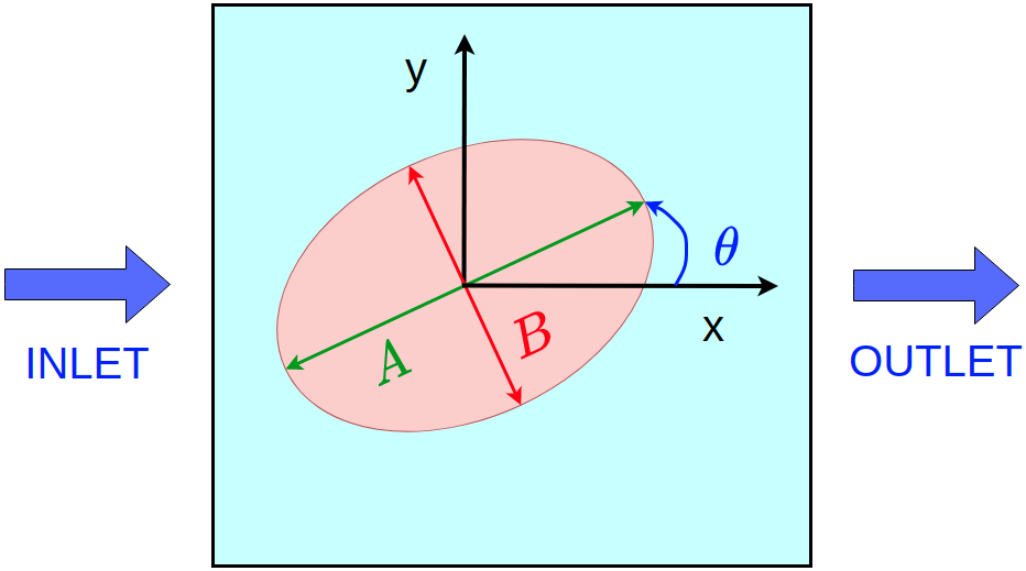
(a) Case of Single Elliptic Cylinder

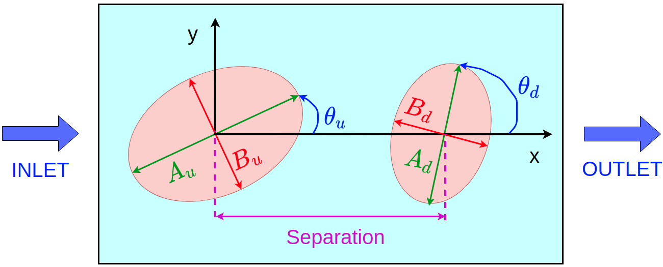
(b) Case of Double Elliptic Cylinder

Figure 1: Schematic of the Flow Domain in the Vicinity of the Cylinders (Cylinder Dimensions Artificially Enlarged)

The top and bottom boundaries are specified to have the free stream velocities with no-slip conditions on the surfaces of the elliptic cylinders. Uniform unit normal and zero transverse velocities are prescribed at the inlet. Constant pressure is imposed at the outlet. The drag and lift coefficients are defined as

$$C_{L}=\frac{F_{D}}{0.5\rho U^{2}A}\hskip 28.45274ptC_{L}=\frac{F_{L}}{0.5\rho U^{2}A}$$ (1)

where, $F_{D}$ and $F_{L}$ are drag and lift forces per unit length respectively and $A$ is taken to be the length of the major axis. Both pressure and viscous forces are included in calculation of drag and lift forces.

The computations are ensured to have low discretization errors by preforming simulations on three different grids, as shown in figs. 2 and 3 for the region around cylinders. The finest grid is used in all the calculations in the following sections. Tables 1 and 2 present the computed lift and drag coefficients for the three grids to show the effects of grid refinement for the single and double cylinder cases respectively. The difference between the medium and finest grids is small, and the finest grid can be considered to give grid-independent results.

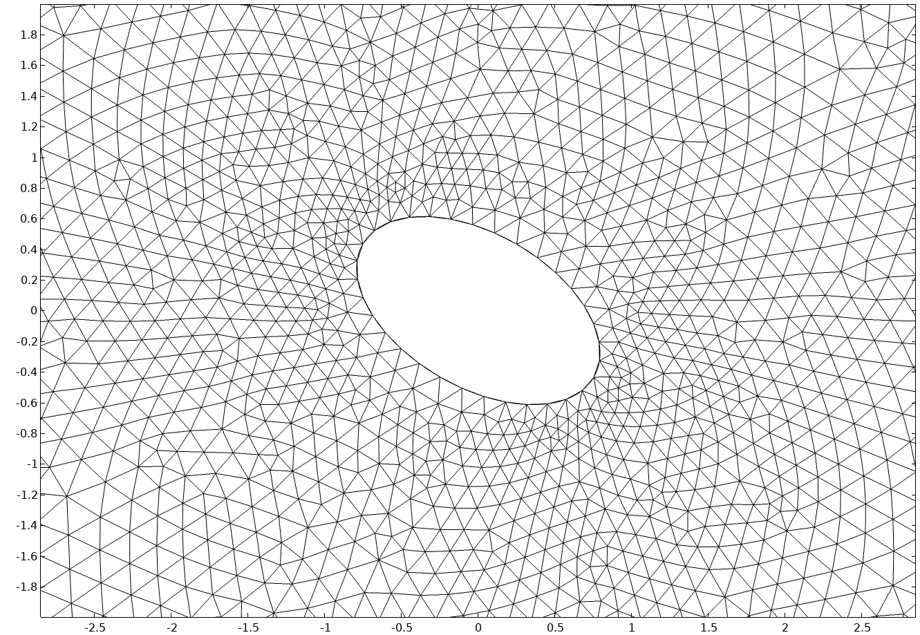
(a) Coarse Mesh (32052 Elements)

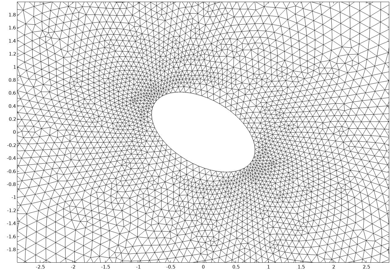
(b) Medium Mesh (113198 Elements)

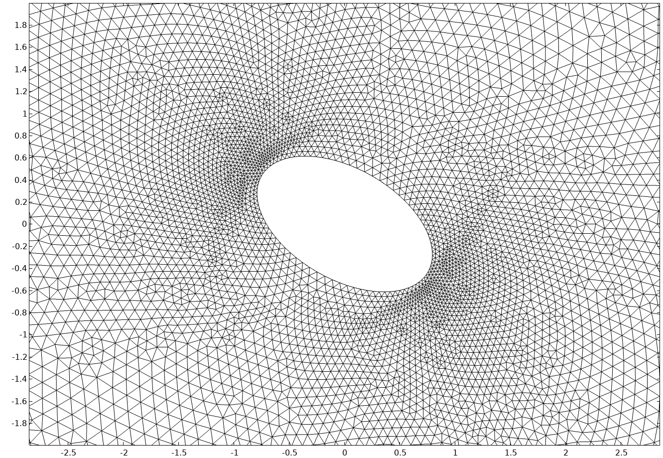
(c) Fine Mesh (451098 Elements)

Figure 2: Single Cylinder Case: Successively Refined Meshes for Grid-Independence Study

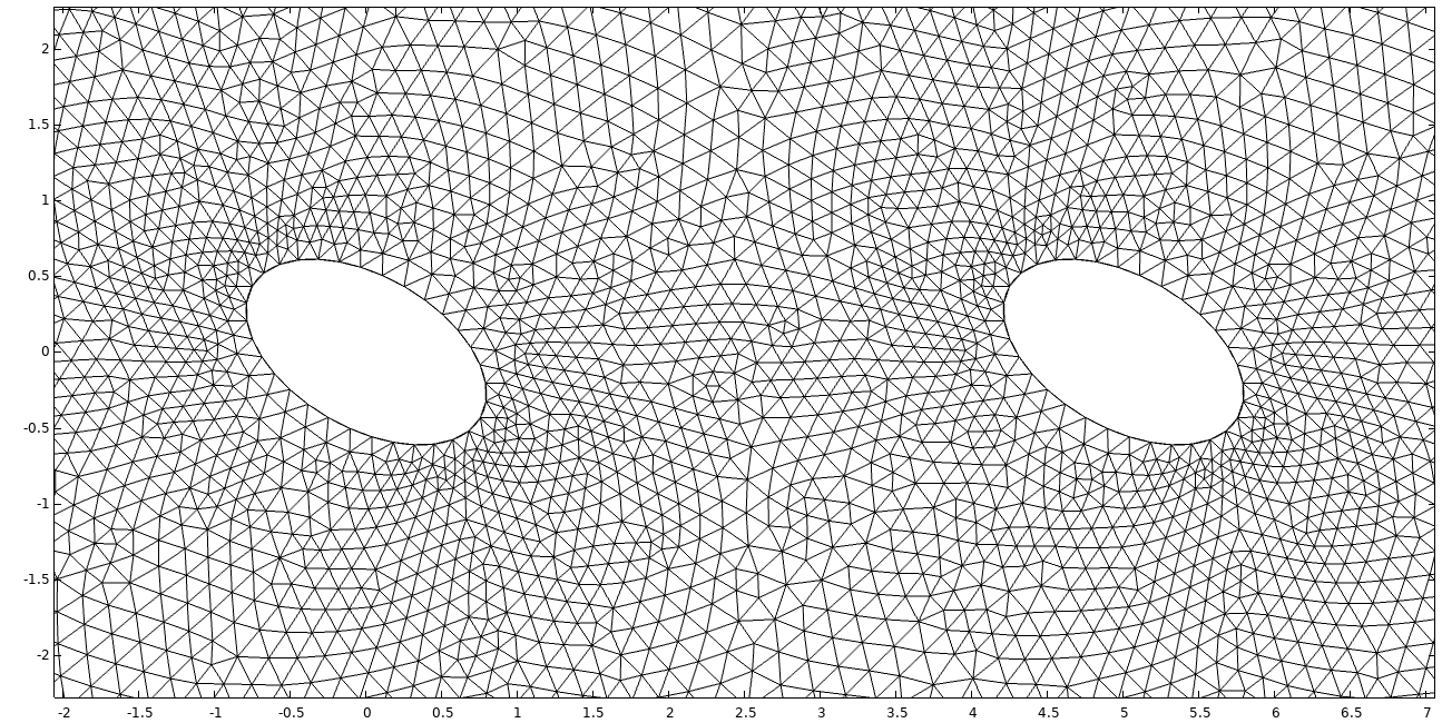
(a) Coarse Mesh (32052 Elements)

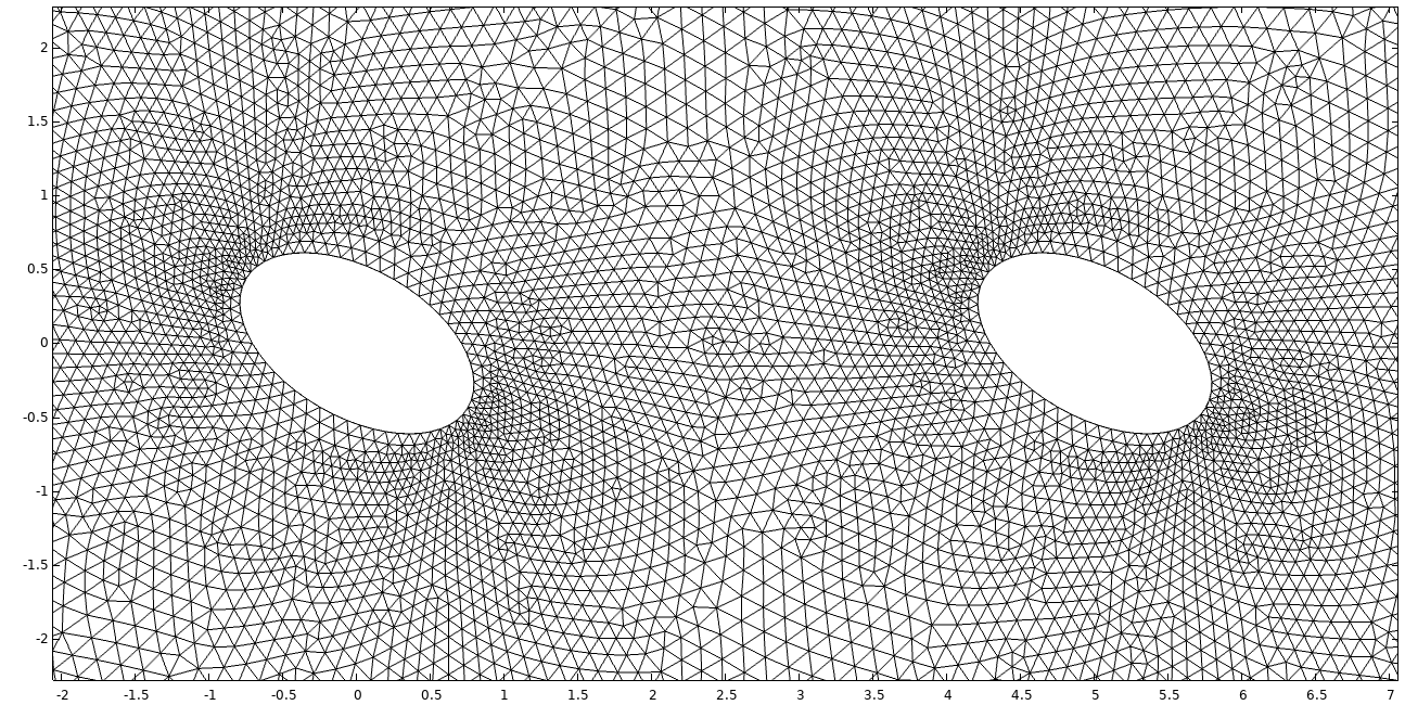
(b) Medium Mesh (118938 Elements)

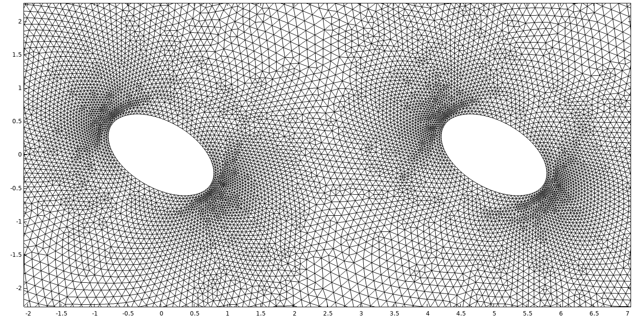
(c) Fine Mesh (457333 Elements)

Figure 3: Double Cylinder Case: Successively Refined Meshes for Grid-Independence Study

	Lift	Drag
Coarse Mesh	0.3868	1.2160
Medium Mesh	0.3895	1.2289
Fine Mesh	0.3903	1.2306

Table 1: Single Cylinder Case: Lift and Drag Coefficients for 3 Refined Grids

	Lift Upstream	Drag Upstream	Lift Downstream	Drag Downstream
Coarse Mesh	0.3797	1.5202	0.1239	0.5510
Medium Mesh	0.3815	1.5341	0.1225	0.5550
Fine Mesh	0.3817	1.5358	0.1215	0.5560

Table 2: Double Cylinder Case: Lift and Drag Coefficients for 3 Refined Grids

3 Multilayer Perceptron Neural Network (MLPNN) for Prediction of Lift and Drag Coefficients

A perceptron, also known as neuron, is a building block of the network. A neuron performs linear transformation on the input vector followed by an element-wise nonlinear activation function to give an output. MLPNN is one of the simplest neural network architectures where neurons are stacked together to form a layer and multiple layers are combined to form a deep network. The linear transformation requires weights and biases which are estimated during the training process by minimizing the loss function. In this work, the mean squared error between estimates obtained from the numerical simulations and predictions of the neural network is defined as the loss function. Hyper-parameters such as number of layers, number of neurons, learning rate etc., are fine tuned by randomly splitting the data into two subsets: training and validation. We use 90% data for training and 10% for validation. A smaller network with few hidden neurons and layers does not fit the training data satisfactorily. This phenomenon is known as under-fitting or bias. Adding more neurons and layers increases the nonlinearity and thus, improves the prediction capability of the network. However, excessively deep networks tend to fit the training data with high accuracy but fail to generalize on unseen validation data. This is known as over-fitting or variance. In practice, a network with low bias and low variance is desired. This is achieved by using the validation data. The trained network is tested on an unseen dataset. A well trained network should perform satisfactorily on both training and testing sets i.e., it should demonstrate low errors and high accuracies on both the sets. More details of the network architecture, training procedure, back-propagation algorithm etc. can be found in the literature [1, 55]. In this work, we have used the open source Python library TensorFlow [56] with its high level API Keras [57].

Lift and drag coefficients are estimated as a function of Reynolds number and geometric parameters using the MLPNN architecture. For the case of a single elliptic cylinder, Reynolds number, angle of attack and ratio of major to minor axis are the three independent input parameters which affect the lift and drag coefficients of the elliptic cylinder (fig. 4(a)). For the second case of double elliptic cylinder, the separation between them is an additional input parameter together with individual angles of attack and ratios (fig. 4(b)). The Reynolds number is defined with respect to the upstream elliptic cylinder. The Reynolds number, angle of attack, aspect ratio and separation are varied in the ranges $[20,40]$, $[0^{\text{o}},180^{\text{o}}]$, $[1,3]$ and $[4,10]$ respectively. The range of Reynolds number is chosen such that a steady state solution exists for the lowest aspect ratio of unity. For a circular cylinder, the critical Reynolds number is around 42.

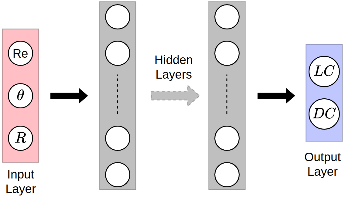
(a) Case of Single Elliptic Cylinder

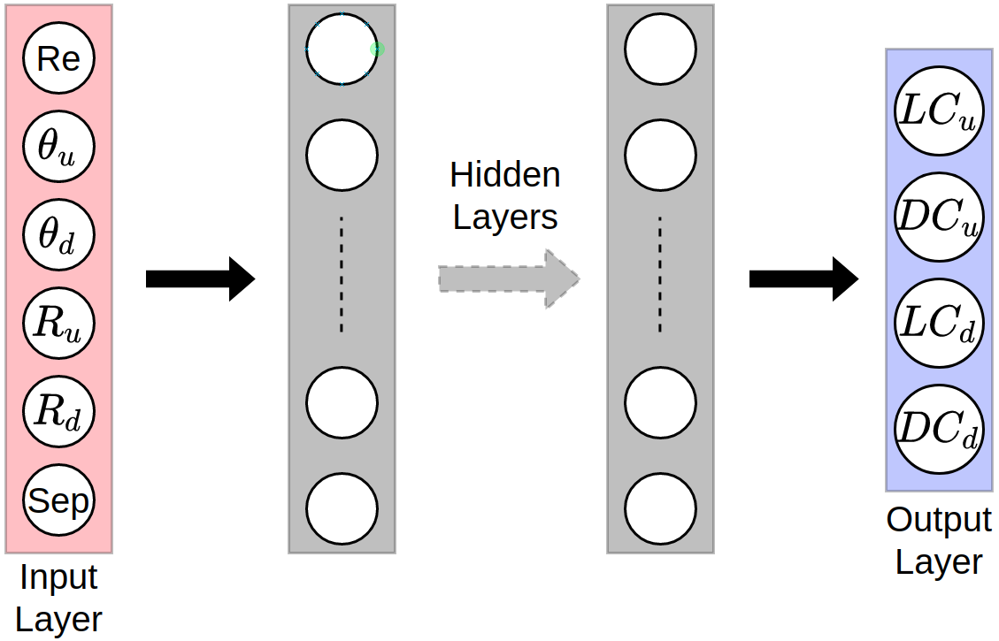
(b) Case of Double Elliptic Cylinder

Figure 4: MLPNN for Estimation of Lift and Drag Coefficients ($LC$: lift coefficient, $DC$: drag coefficient, $Re$: Reynolds no., $\theta$: angle of attack, $R$: ratio of major to minor axis, Sep: separation between ellipse centers, subscript $u$: upstream, subscript $d$: downstream)

	Case of Single Elliptic Cylinder	Case of Double Elliptic Cylinder
No. of Hidden Layers	6	8
No. of Neurons per Hidden Layer	100	200
No. of Trainable Parameters	51,102	286,804
Learning Rate	0.002	0.1
Optimization Algorithm	Adam [58]	Adam [58]
No. of Epochs	1000	10000
Loss Function	Mean Squared Error	Mean Squared Error
Hidden Layers Activation	ReLU	ReLU
Output Layer Activation	Linear	Linear
Size of Training Set	1100	3500
Size of Testing Set	100	200

Table 3: Hyper-Parameters of MLPNN

Hyper-parameters of the MLPNN for both the cases are listed in table 3. These hyper-parameters are tuned by using 10% of the training data for validation. The trained network is tested on a separate unseen dataset. For a dataset with sample size $m$, let $\bm{y}^{s}=[y_{1}^{s},y_{2}^{s},\dots,y_{m}^{s}]$ and $\bm{y}^{n}=[y_{1}^{n},y_{2}^{n},\dots,y_{m}^{n}]$ denote predictions of the variable $y$ using numerical simulations and neural networks respectively. The coefficient of determination ($R^{2}$) [59] is used to estimate accuracy of the neural networks.

$$\text{Accuracy: }R^{2}=1-\frac{\sum_{i=1}^{m}(y_{i}^{s}-y_{i}^{n})^{2}}{\sum_{i=1}^{m}(y_{i}^{s}-\text{mean}(\bm{y}^{s}))^{2}}$$ (2)

Percentage errors are defined as follows:

$$\text{Average percent error: }100\times\frac{1}{m}\frac{\sum_{i=1}^{m}||y_{i}^{s}-y_{i}^{n}||}{\max_{i=1}^{m}||y_{i}^{s}||}$$ (3)

$$\text{Maximum percent error: }100\times\frac{\max_{i=1}^{m}||y_{i}^{s}-y_{i}^{n}||}{\max_{i=1}^{m}||y_{i}^{s}||}$$ (4)

		Single Elliptic Cylinder		Double Elliptic Cylinder
				Upstream		Downstream
		Lift	Drag	Lift	Drag	Lift	Drag
Accuracy	Training	0.999936	0.999954	0.998668	0.998507	0.997685	0.998775
	Testing	0.999791	0.999821	0.997543	0.998020	0.988764	0.997606
Average Percent Error	Training	0.3050	0.0717	1.317	0.4091	0.6759	0.4286
	Testing	0.5495	0.1333	1.699	0.4508	1.239	0.6132
Maximum Percent Error	Training	1.327	0.3679	6.807	6.235	6.706	2.609
	Testing	2.063	0.9228	11.18	2.406	17.90	4.748

Table 4: Accuracy and Error of MLPNN

The error and accuracy for training and testing sets are listed in table 4. For a perfect model which fits the data exactly, $R^{2}$ takes a value of unity [59]. In the case of practical models, $R^{2}$ is always less than unity. $R^{2}$ value close to unity indicates high accuracy. Thus, low errors and high accuracy show that the networks are successful in estimating the lift and drag coefficients for both the cases. Moreover, similar error estimates for training and testing sets indicate that the chosen hyper-parameters are optimal and the networks have low variance. The estimates of drag and lift coefficients obtained from numerical simulations and neural networks for testing datasets are plotted in figs. 5 and 6. Both the axes are scaled to range $[0,1]$ using the minimum and maximum values of the numerical estimates. It can be seen that most of the points lie on the ideal trend line $y=x$ indicating high accuracy of the networks. It should be noted that there are always a few outliers which show slightly higher values of maximum percent errors in table 4.

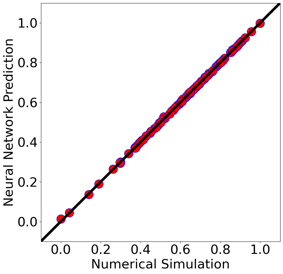
(a) Single Elliptic Cylinder

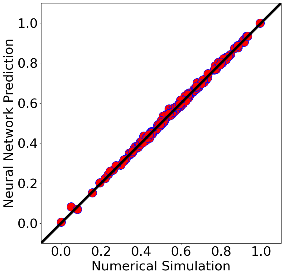
(b) Double Elliptic Cylinder: Upstream

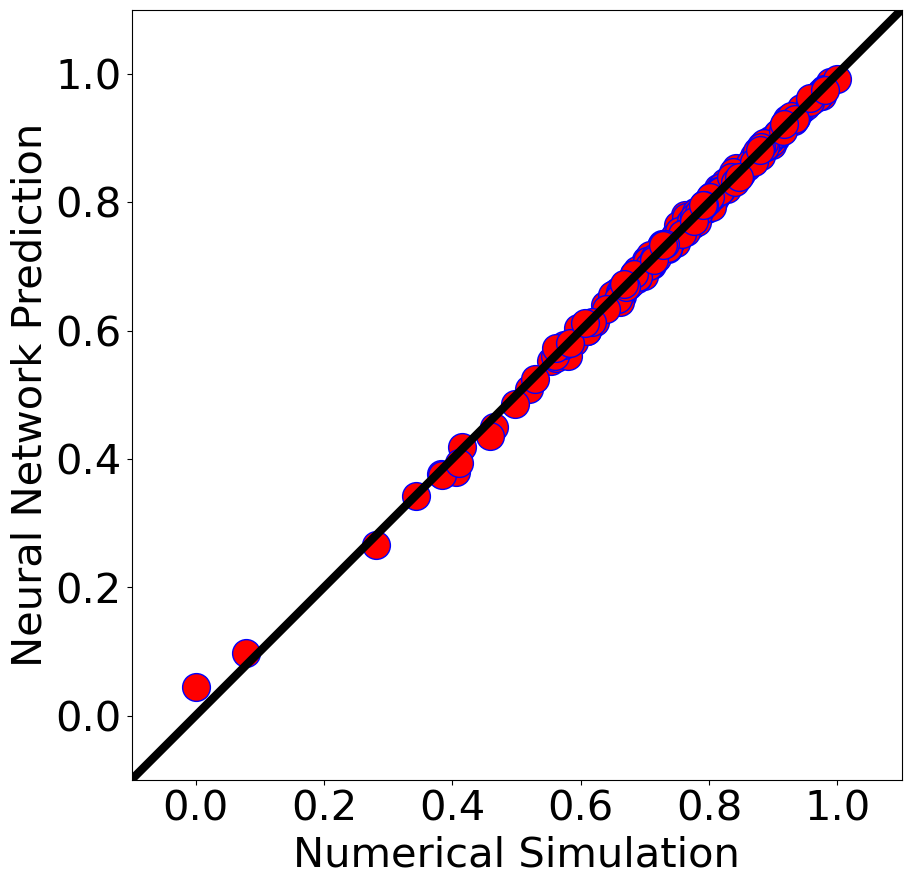
(c) Double Elliptic Cylinder: Downstream

Figure 5: Drag Coefficient (Scaled): Comparison of Numerical Simulation and Neural Network Prediction

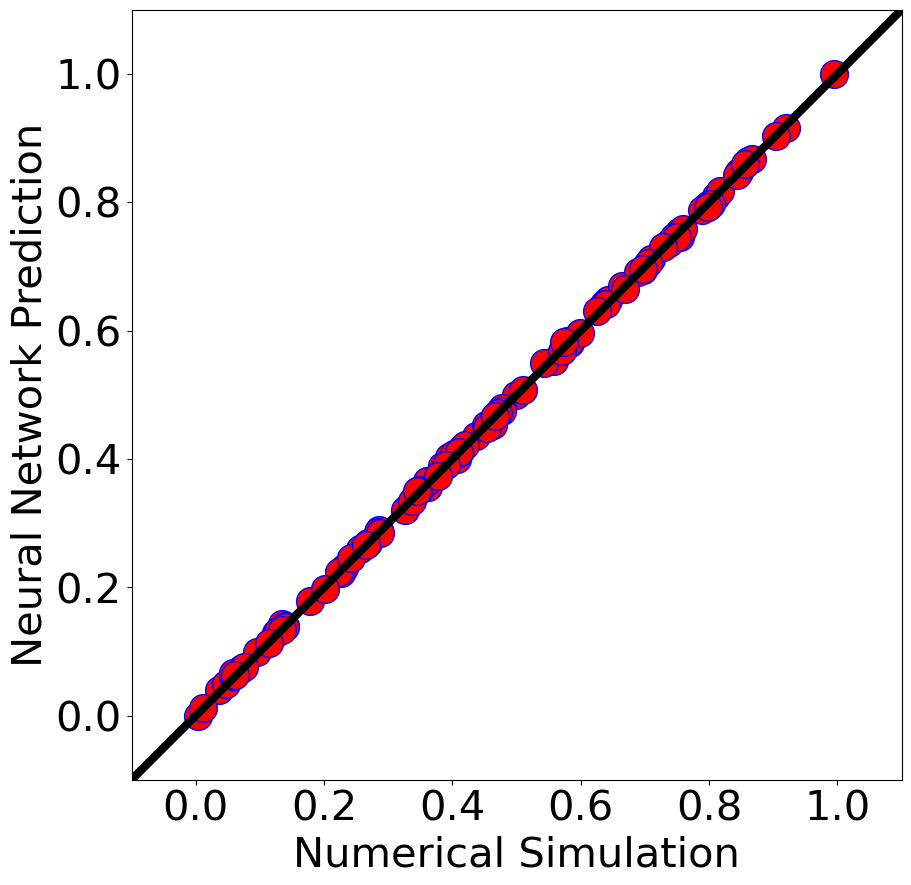
(a) Single Elliptic Cylinder

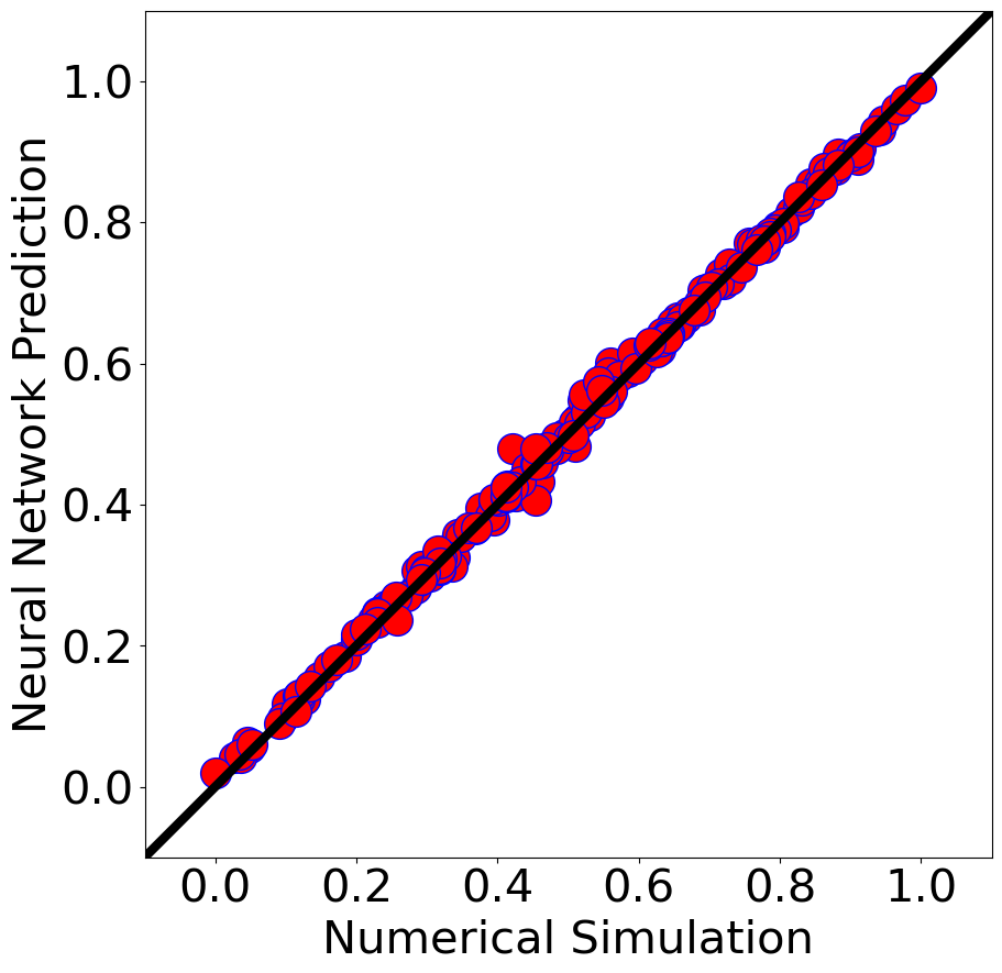
(b) Double Elliptic Cylinder: Upstream

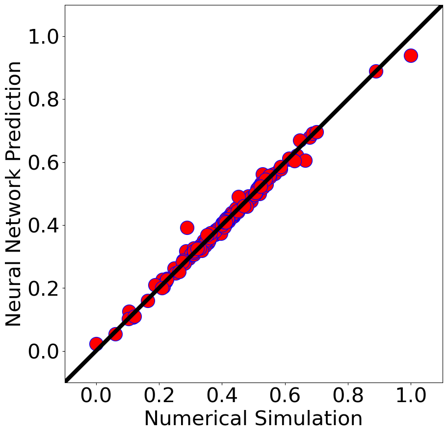
(c) Double Elliptic Cylinder: Downstream

Figure 6: Lift Coefficient (Scaled): Comparison of Numerical Simulation and Neural Network Prediction

4 Variation of Lift and Drag Coefficients

The MLPNN is now used to study the variation of lift and drag coefficients with aspect ratio, angle of attack and the flow Reynolds number. A pictorial variation as contour plots is first shown in figs. 7 and 8. Figure 7 shows the lift coefficients with angle of attack and aspect ratio as coordinate axes. The angle of $0^{\text{o}}$ corresponds to a horizontal placement of the major axis, and the angle of attack is measured counterclockwise. An angle of $90^{\text{o}}$ corresponds to the case of major axis being vertical. As can be expected, the lift coefficients for $0^{\text{o}}$, $90^{\text{o}}$, and $180^{\text{o}}$ angles of attack are zero, with maximum lift coefficients occurring around $45^{\text{o}}$ and $135^{\text{o}}$. Moreover, for angle of attack of between $[0^{\text{o}},90^{\text{o}}]$, the major axis points in the first and third quadrant. Hence, the lift is negative since the force is acting in the downward direction.

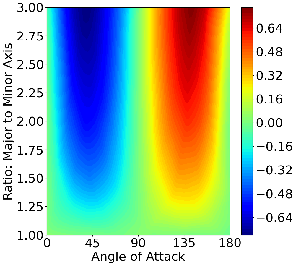
(a) Reynolds No.: 20

(b) Reynolds No.: 30

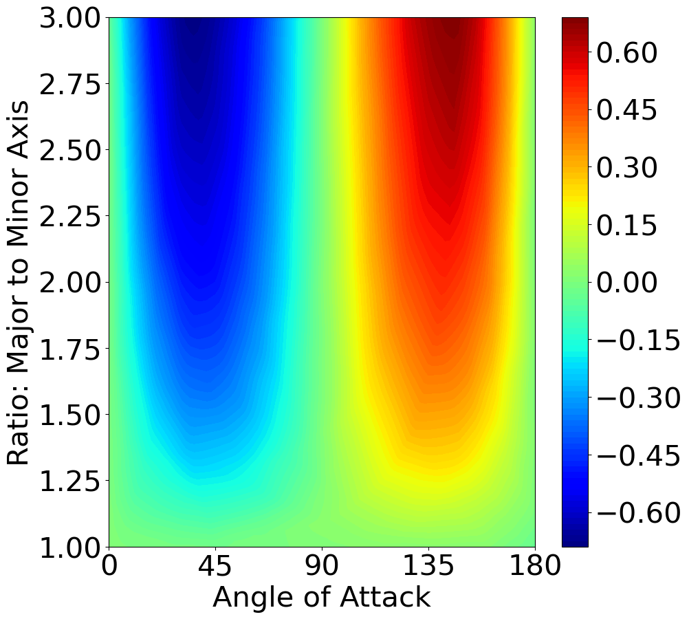
(c) Reynolds No.: 40

Figure 7: Case of Single Elliptic Cylinder: Lift Coefficient

Figure 8 shows the variation of the drag coefficient at the same three Reynolds numbers. The drag coefficient is always maximum at 90 degrees. The drag is the same for all angles of attack for the aspect ratio of unity (circular cylinder). For non-unity aspect ratios, the drag increases with angle of attack between $0^{\text{o}}$ and $90^{\text{o}}$, and then decreases between $90^{\text{o}}$ and $180^{\text{o}}$. The drag also increases with aspect ratio for any angle of attack. The drag, which includes both pressure drag and viscous shear stress, decreases with Reynolds number because of the lower viscosity. The present Reynolds number range is limited to a value for which all angles of attack give a steady flow.

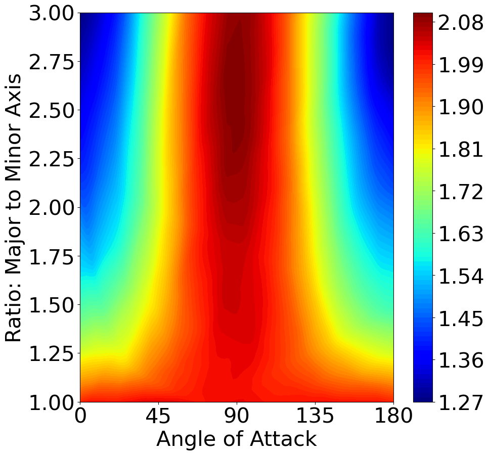
(a) Reynolds No.: 20

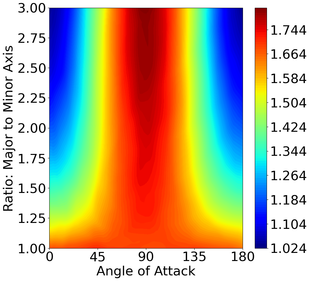
(b) Reynolds No.: 30

(c) Reynolds No.: 40

Figure 8: Case of Single Elliptic Cylinder: Drag Coefficient

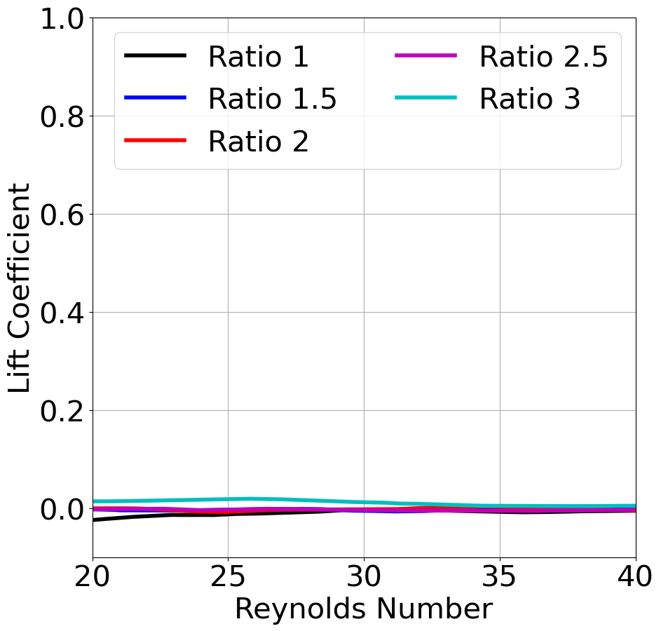
(a) Angle of Attack: $90^{0}$

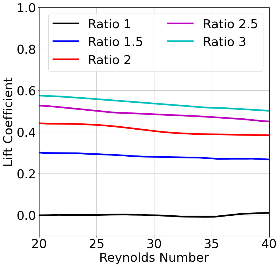
(b) Angle of Attack: $120^{0}$

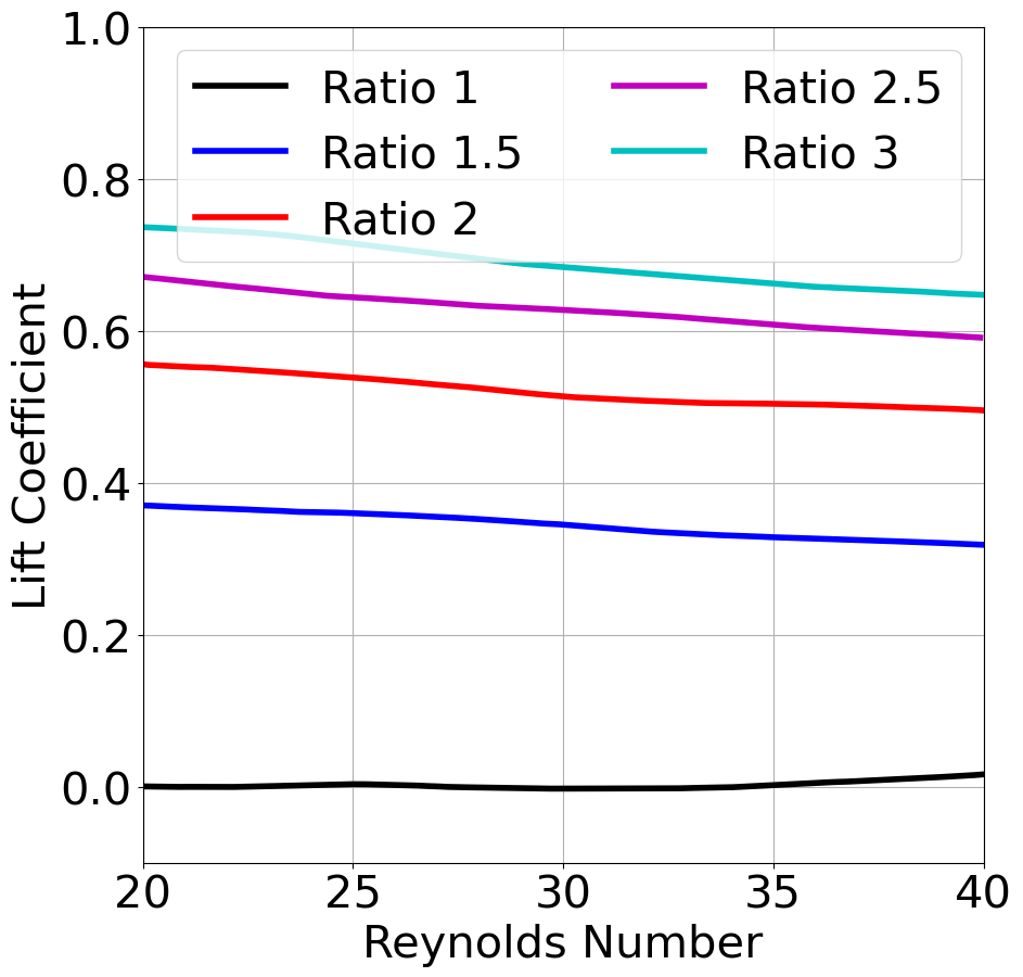
(c) Angle of Attack: $135^{0}$

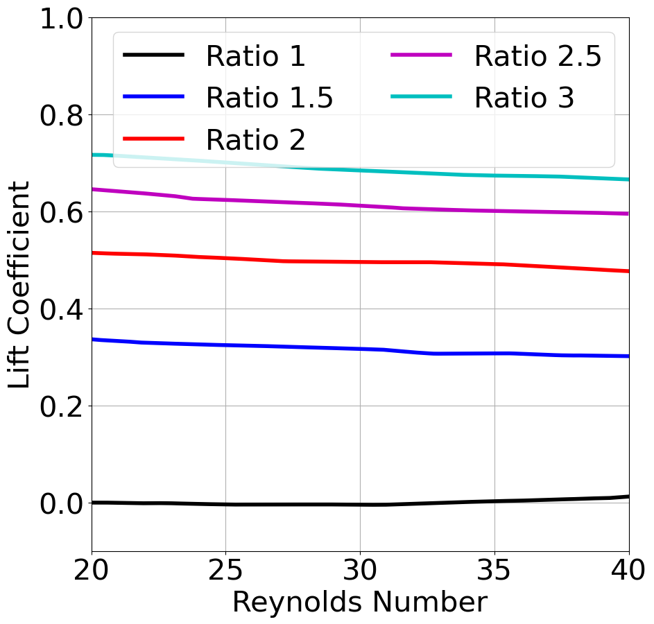
(d) Angle of Attack: $150^{0}$

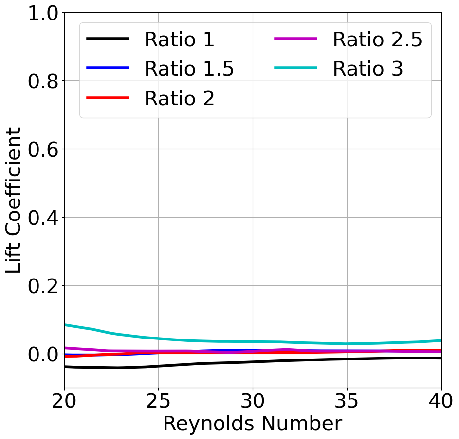
(e) Angle of Attack: $180^{0}$

Figure 9: Case of Single Elliptic Cylinder: Lift Coefficient

We now discuss the variations in lift and drag coefficients by studying the trends through line plots. Figure 9 shows the lift coefficient for various angles of attack as a function of the Reynolds number. We first observe that the neural network gives the lift coefficient for angles of attack of $0^{\text{o}}$, $90^{\text{o}}$ and $180^{\text{o}}$ to be nearly zero within a few percent error. For other angles between $90^{\text{o}}$ and $180^{\text{o}}$, the lift coefficient is positive, and increases with aspect ratio. As the body becomes slimmer and slimmer, the separation length and the low pressure on the back side of the body increase, thus increasing the lift coefficient. Also, the surface area over which the pressure and normal stress forces act also increases. Thus, the lift coefficient becomes larger as the angle of attack passes $90^{\text{o}}$. The effect of the aspect ratio is always seen to be monotonic for all angles of attack.

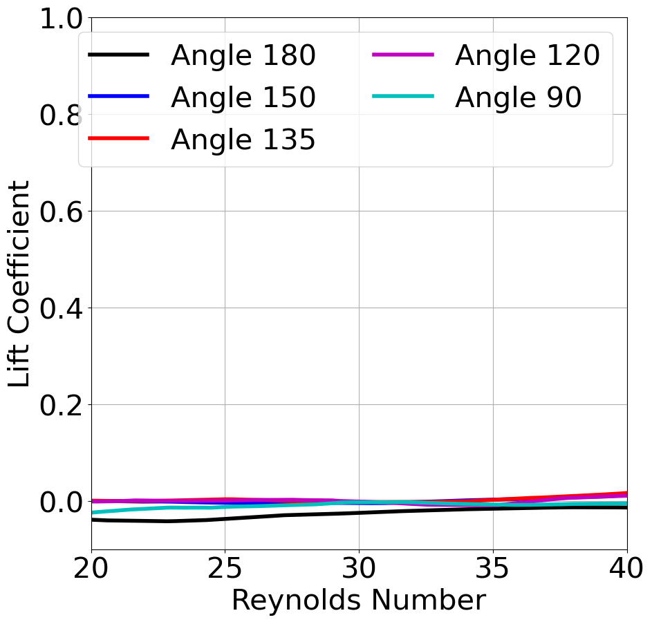
(a) Ratio: Major/Minor Axis: 1

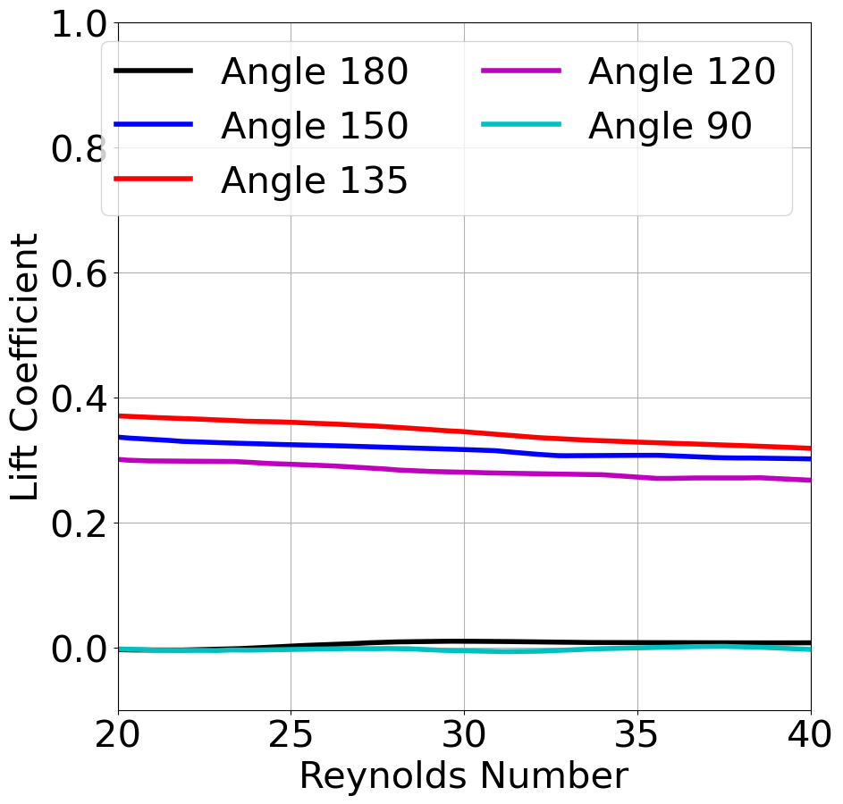
(b) Ratio: Major/Minor Axis: 1.5

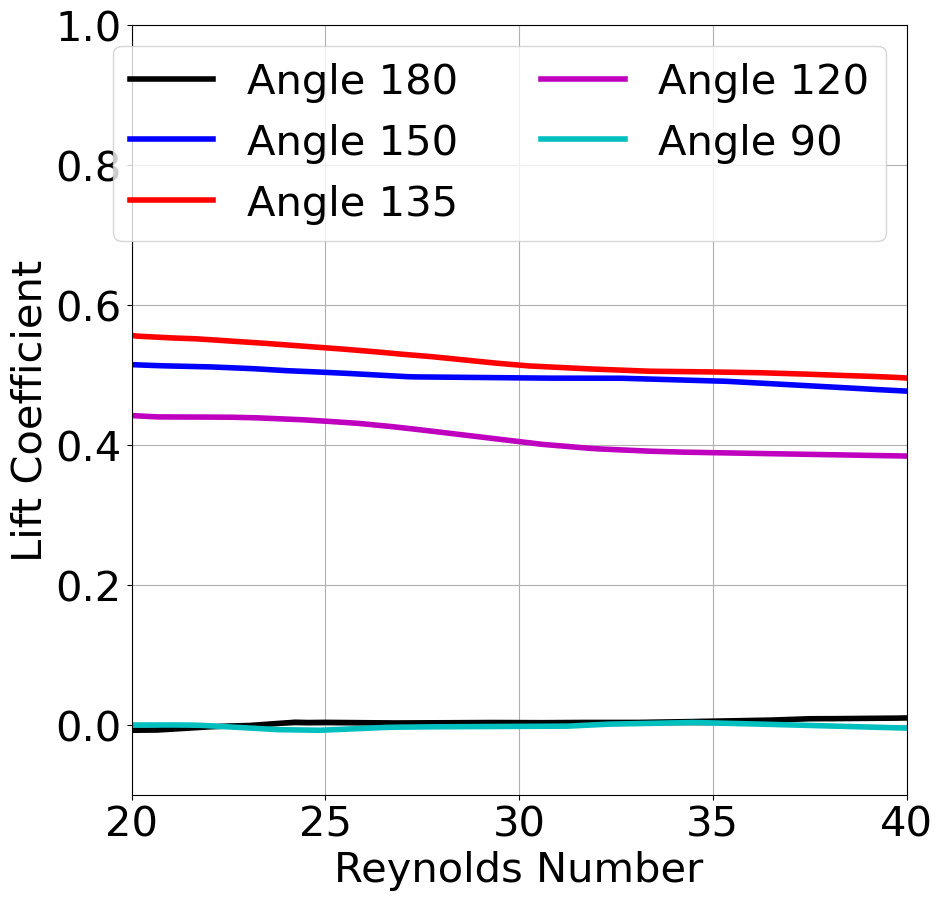
(c) Ratio: Major/Minor Axis: 2

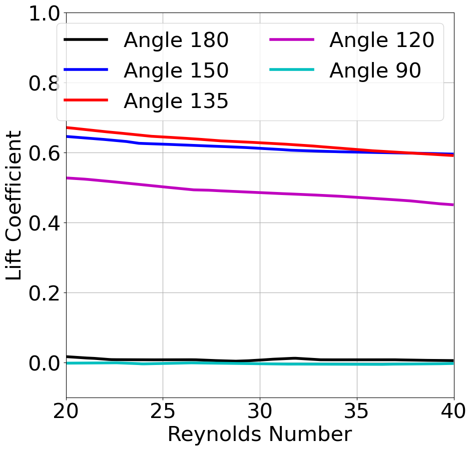
(d) Ratio: Major/Minor Axis: 2.5

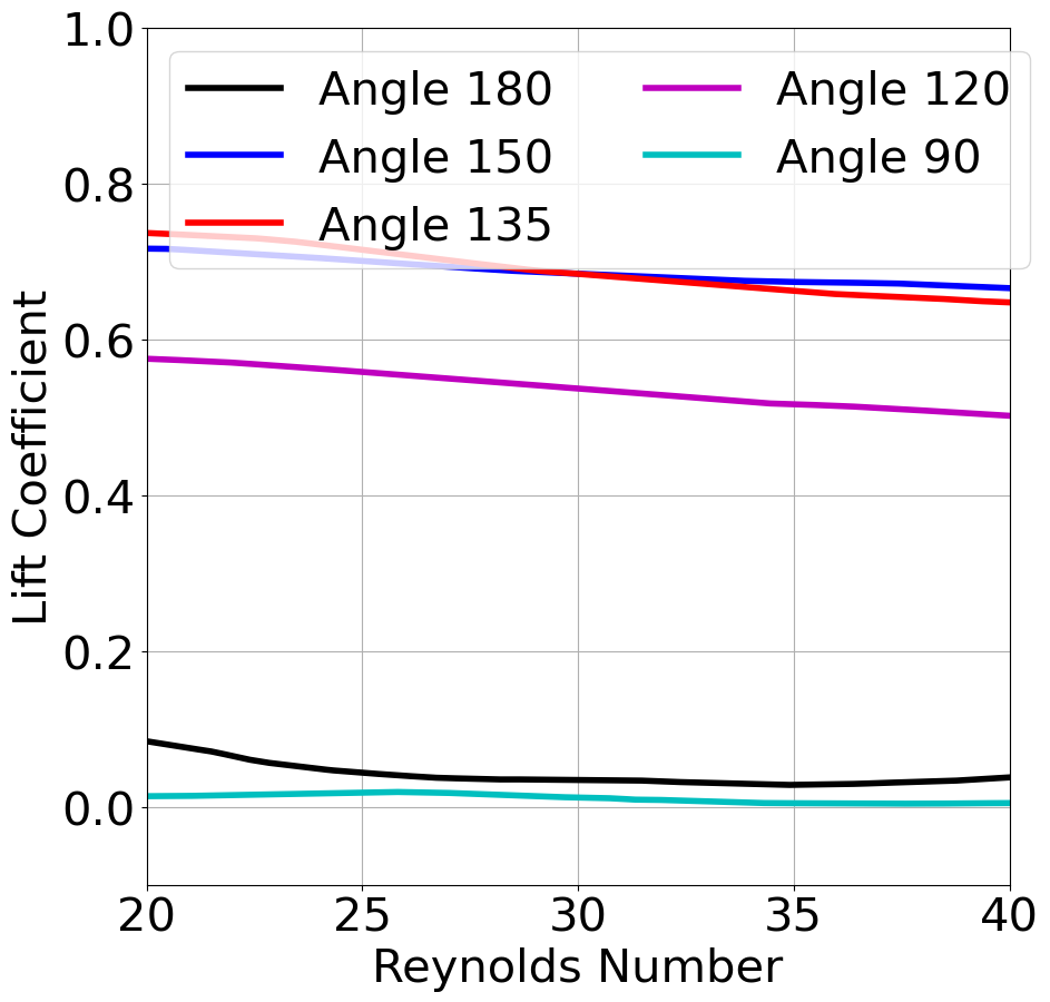
(e) Ratio of Major/Minor Axis: 3

Figure 10: Case of Single Elliptic Cylinder: Lift Coefficient

It is also instructive to plot the variations of the lift coefficient as a function of the Reynolds number. This effect is seen to be somewhat weak, as negative pressure on the back side of the cylinder decreases only slightly with the Reynolds number. However, as seen earlier, the angle of attack has a predominant effect on the lift coefficient. Surprisingly, the lift coefficients for angle of attack of $150^{\text{o}}$ and $135^{\text{o}}$ are nearly the same for all aspect ratios. This is particularly the case for aspect ratios of two and greater.

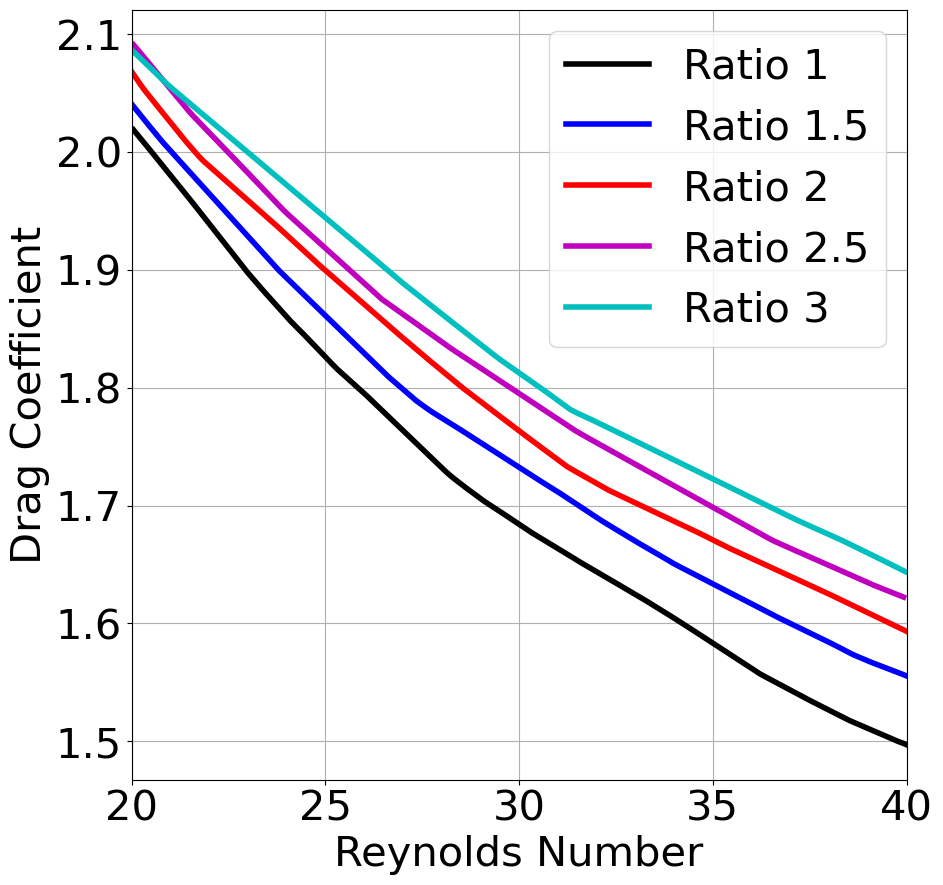
(a) Angle of Attack: $90^{0}$

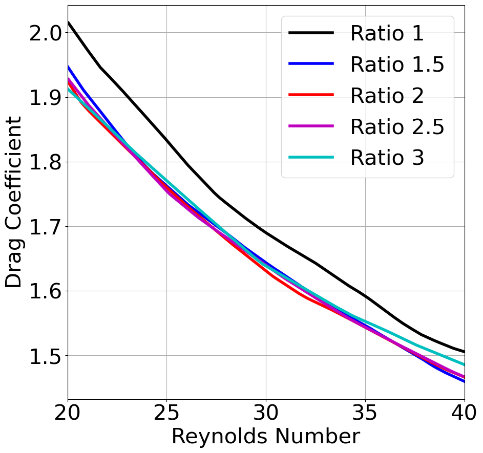
(b) Angle of Attack: $120^{0}$

(c) Angle of Attack: $135^{0}$

(d) Angle of Attack: $150^{0}$

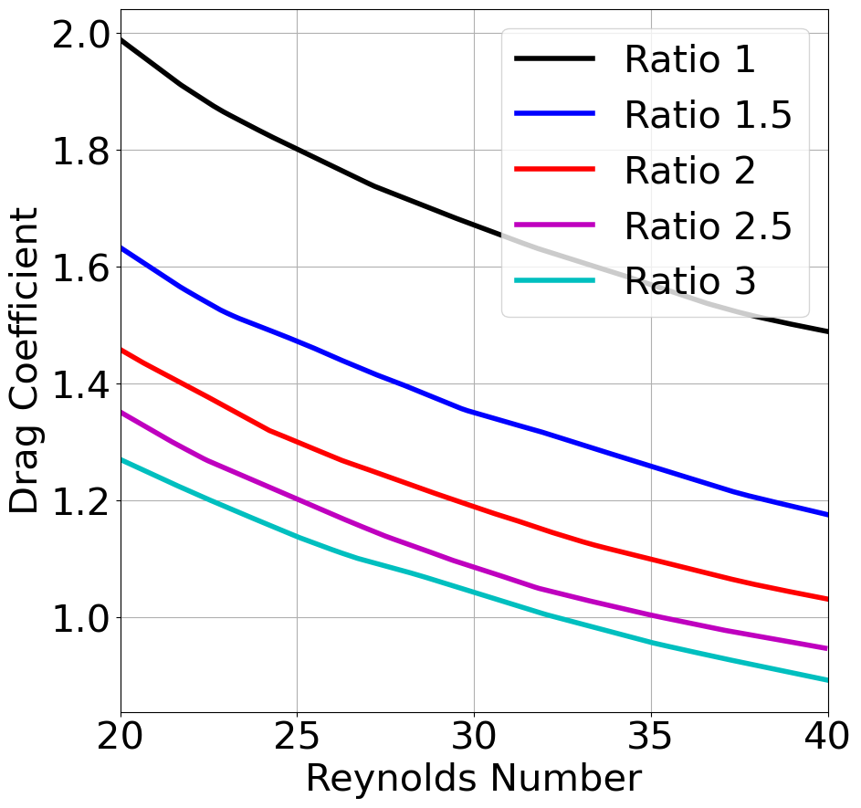
(e) Angle of Attack: $180^{0}$

Figure 11: Case of Single Elliptic Cylinder: Drag Coefficient

The effect of Reynolds number on the drag coefficient, for various angles of attack, is shown in fig. 11 for different aspect ratios. First, for the case of unity aspect ratio, there is no effect of the angle of attack since it is a circular cylinder. The drag coefficient is the same at all angles of attack and reduces with Reynolds number. For non-unity aspect ratios, interesting trends are observed. For a vertical alignment ($90^{\text{o}}$), the drag monotonically increases with aspect ratios. However, as the cylinder is rotated counterclockwise to higher angles, the curves cross those of the circular cylinder and predict a lower drag coefficient. at an angle of attack of $120^{\text{o}}$, we see that the drag for all aspect ratios higher than unity is almost similar. When the cylinder reaches a horizontal position ($180^{\text{o}}$), the drag becomes significantly smaller than the circular cylinder due to streamlined body. As the aspect ratio is increased, the cylinder tends to get slimmer, so the drag due to wake formation and skin friction is reduced.

For tandem cylinders, there are six parameters, and hence the lift and drag coefficients vary over a six-dimensional space. It is difficult to analyze the variations in a six dimensional input space due to a complex interactions between these inputs. Hence, we have arbitrarily selected two cases to demonstrate what can be obtained from the trained neural networks. It can be seen that some variations seem to be linear whereas others show a significantly nonlinear behavior. We also observe that the coefficients on the downstream cylinder are substantially different than the upstream cylinder which shows that the upstream cylinder perturbs the uniform flow field. We are currently developing a graphical interface which can be used to maneuver the complete space and easily compute the parametric variations. This interface can be used as a virtual laboratory experiment in fluid mechanics education.

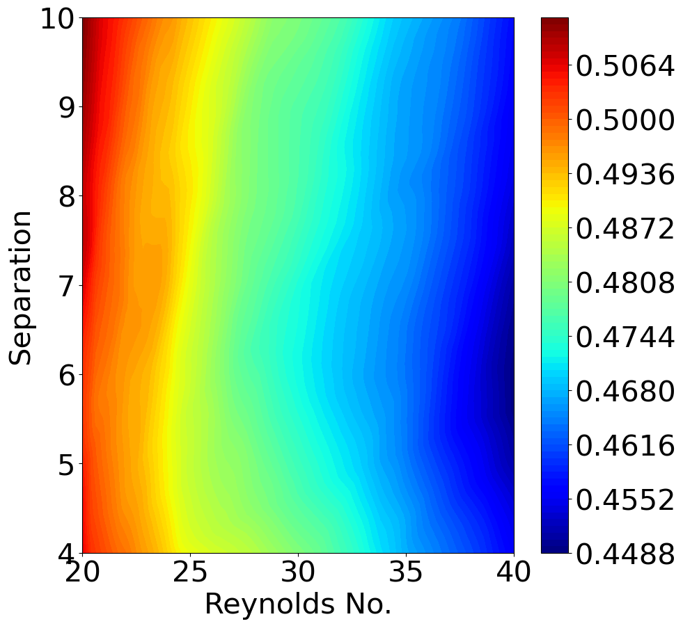
(a) Upstream and Downstream Angles: $135^{0}$

(b) Upstream Angle: $90^{0}$, Downstream Angle: $135^{0}$

(c) Upstream Angle: $135^{0}$, Downstream Angle: $90^{0}$

Figure 12: Case of Double Elliptic Cylinder: Lift Coefficient of Upstream Cylinder (Upstream and Downstream Aspect Ratio: 2)

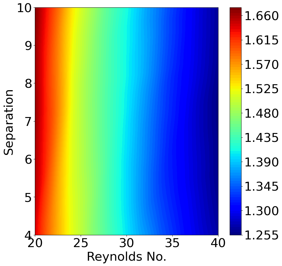
(a) Upstream and Downstream Angles: $135^{0}$

(b) Upstream Angle: $90^{0}$, Downstream Angle: $135^{0}$

(c) Upstream Angle: $135^{0}$, Downstream Angle: $90^{0}$

Figure 13: Case of Double Elliptic Cylinder: Lift Coefficient of Downstream Cylinder (Upstream and Downstream Aspect Ratio: 2)

(a) Upstream and Downstream Angles: $135^{0}$

(b) Upstream Angle: $90^{0}$, Downstream Angle: $135^{0}$

(c) Upstream Angle: $135^{0}$, Downstream Angle: $90^{0}$

Figure 14: Case of Double Elliptic Cylinder: Drag Coefficient of Upstream Cylinder (Upstream and Downstream Aspect Ratio: 2)

(a) Upstream and Downstream Angles: $135^{0}$

(b) Upstream Angle: $90^{0}$, Downstream Angle: $135^{0}$

(c) Upstream Angle: $135^{0}$, Downstream Angle: $90^{0}$

Figure 15: Case of Double Elliptic Cylinder: Drag Coefficient of Downstream Cylinder (Upstream and Downstream Aspect Ratio: 2)

5 Sensitivity Analysis

Sensitivity can be defined as the effect of perturbation of an input on an output. Let $Y$ be a scalar output dependent on a $d$ dimensional input vector $\bm{X}=[X_{1},X_{2},\dots X_{d}]$. Let $f$ denote the model which relates $\bm{X}$ to $Y$ i.e., $Y=f(\bm{X})$. For instance, in the case of single elliptic cylinder, drag coefficient is a particular output ($Y$) as a function of inputs such as Reynolds number, ratio and angle of attack (3 dimensional vector $\bm{X}$) and the neural network is used as the model ($f$). Partial derivative of $Y$ with respect to a particular input $X_{i}$ is one way to define the sensitivity of $Y$ to $X_{i}$. Since the partial derivative has to be evaluated at a particular value of $\bm{X}=\bm{\hat{X}}$, this gives an estimate of the local sensitivity at $\bm{\hat{X}}$. Response surfaces can be used to visualize local sensitivity. For example, slope of the contour lines in the fig. 8(a) is low for ratio of 1.25 and $0^{\text{o}}$ angle of attack. Hence, in this region, the drag is more sensitive to the ratio than angle of attack. On the other hand, in the region of 2.5 ratio and $45^{\text{o}}$ angle of attack, the contours are steep indicating that the drag is more sensitive to the angle. This example demonstrates that the partial derivatives can vary significantly from one design point to another due to the nonlinearity of the model. Hence, for practical problems with nonlinear relationships, the local sensitivity analysis does not give any information of the entire design space.

In this work, we use the variance based analysis, also known as Sobol method [60] to estimate the global sensitivities of each output with respect to each input. The relation $Y=f(\bm{X})$ can be written as a summation of functions over individual inputs:

$$Y=f(\bm{X})=f_{0}+\sum_{i=1}^{d}f_{i}(X_{i})+\sum_{i<j}^{d}f_{i,j}(X_{i},X_{j})+\dots+f_{1,2,\dots,d}(X_{1},X_{2},\dots X_{d})$$ (5)

where, $f_{0}$ is a constant, $f_{i}$ is a function of single input $X_{i}$, $f_{i,j}$ is a function of two inputs $X_{i}$ and $X_{j}$ and so on. This summation has $2^{d}$ functions for a $d$ dimensional input space. The decomposition is known as ANOVA (analysis of variances) if each of the functions has zero means:

$$\int f_{i_{1},i_{2},\dots,i_{s}}(X_{i_{1}},X_{i_{2}},\dots,X_{i_{s}})dX_{k}=0\hskip 5.69046pt\text{for}\hskip 5.69046ptk=i_{1},i_{2},\dots,i_{s}$$ (6)

It can be shown that if the above condition is satisfied, the functions are orthogonal and thus, the decomposition is unique [61]. If $f(\bm{X})$ is assumed to be square-integrable, squaring eq. 5 and integrating gives:

$$\int Y^{2}d\bm{X}-f_{0}^{2}=\sum_{s=1}^{d}\sum_{i_{1}<\dots<i_{s}}^{d}\int f^{2}_{i_{1},\dots,i_{s}}dX_{i_{1}}\dots X_{i_{s}}$$ (7)

Note that the cross terms such as $\int f_{i_{1}}f_{i_{2}}dX_{i_{1}}dX_{i_{2}}$ are zero due to orthogonality and only the squared terms remain. The left hand side of eq. 7 is equal to variance of $Y$ and the right hand side is a summation of variances due to groups of inputs. Hence, the total variance in $Y$ is decomposed into variances attributed to individual inputs and interactions between them:

$$Var(Y)=\sum_{i=1}^{d}V_{i}+\sum_{i<j}^{d}V_{i,j}+\dots+V_{1,2,\dots,d}$$ (8)

First order sensitivity index is defined as $S_{i}=V_{i}/Var(Y)$. Higher order indices such as $S_{i,j}$ are similarly defined. From eq. 8, it can be seen that these ($2^{d}-1$) indices are non-negative and sum to unity. Total Sobol index ($S_{T_{i}}$) for each input $X_{i}$ is defined as sum of all the first and higher order indices with $X_{i}$ in it. For example, for the case with 3 inputs, $S_{T_{1}}=S_{1}+S_{1,2}+S_{1,3}+S_{1,2,3}$. Note that the sum of total indices is typically more than unity since the interaction terms are counted more than once. In this work, we analyze the total Sobol indices of each output (lift and drag coefficients) with respect to each input (Reynolds number, angle, aspect ratio and separation). For simple functions, the integrals in eq. 7 can be evaluated analytically. For practical cases however, Monte-Carlo methods are used to estimate total Sobol indices. Brute force computation is $\mathcal{O}(N^{2})$ where, $N$ denotes the number of Monte-Carlo samples. Since $N$ can of the order of $10^{5}\sim 10^{6}$, these computations are quite expensive even when surrogate models are used. Hence, we use the algorithm proposed by Saltelli et al. [61] which requires $\mathcal{O}(N(d+2))$ computations.

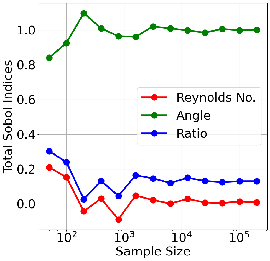
(a) Lift Coefficient

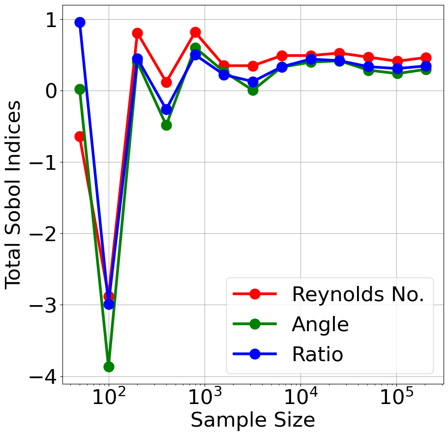
(b) Drag Coefficient

Figure 16: Case of Single Elliptic Cylinder: Estimation of Total Sobol Indices: Convergence of Monte-Carlo Method

The Monte-Carlo method obtains numerical estimates by repeated random sampling. The convergence error is $\mathcal{O}(1/\sqrt{N})$ [62] where, $N$ is the sample size. In the absence of analytical solution, the sample size is increased until the estimates converge asymptotically. For the case of single cylinder, there are two outputs (lift and drag coefficients) and three inputs (Reynolds number, angle, aspect ratio). Thus, convergence of $3\times 2=6$ total Sobol indices is plotted in fig. 16. The sample size is increased exponentially from 50 to 2E5 by a factor of 2 each time. The lift and drag coefficients are estimated as a function of randomly generated sets of inputs using the MLPNN described before. The computational efficiency of neural network facilitates such high sample sizes. This demonstrates the benefit of coupling neural networks with numerical simulations. The initial estimates are inaccurate (sometimes negative) but stationarity is obtained as the sample size reaches close to 1E4. Thus, the average of last 5 estimates is recorded as the converged value. Figure 17 is a bar chart with sensitivity of each output with respect to each input. As discussed before, the sum of total Sobol indices of both outputs is greater than unity. It can be seen that the lift coefficient is highly sensitive to the angle of attack and its dependence on the Reynolds number and aspect ratio is negligible. On the other hand, the drag is more sensitive to the Reynolds number but its sensitivity to the other inputs is also important.

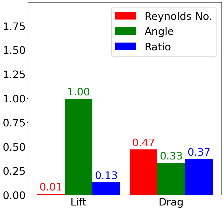
Figure 17: Case of Single Elliptic Cylinder: Total Sobol Indices: Sensitivity of Lift and Drag to 3 Inputs

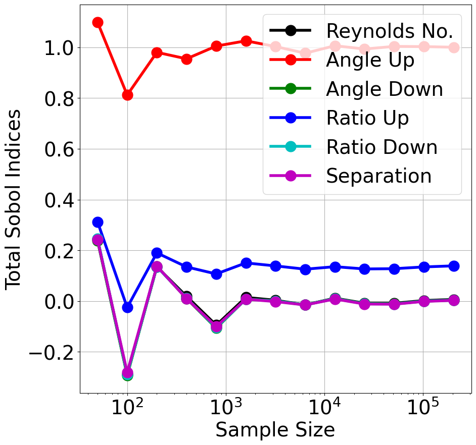
(a) Upstream Lift Coefficient

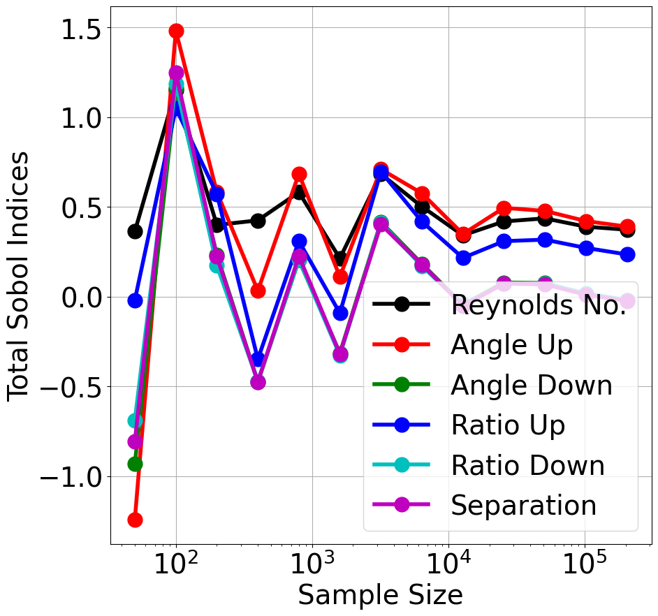
(b) Upstream Drag Coefficient

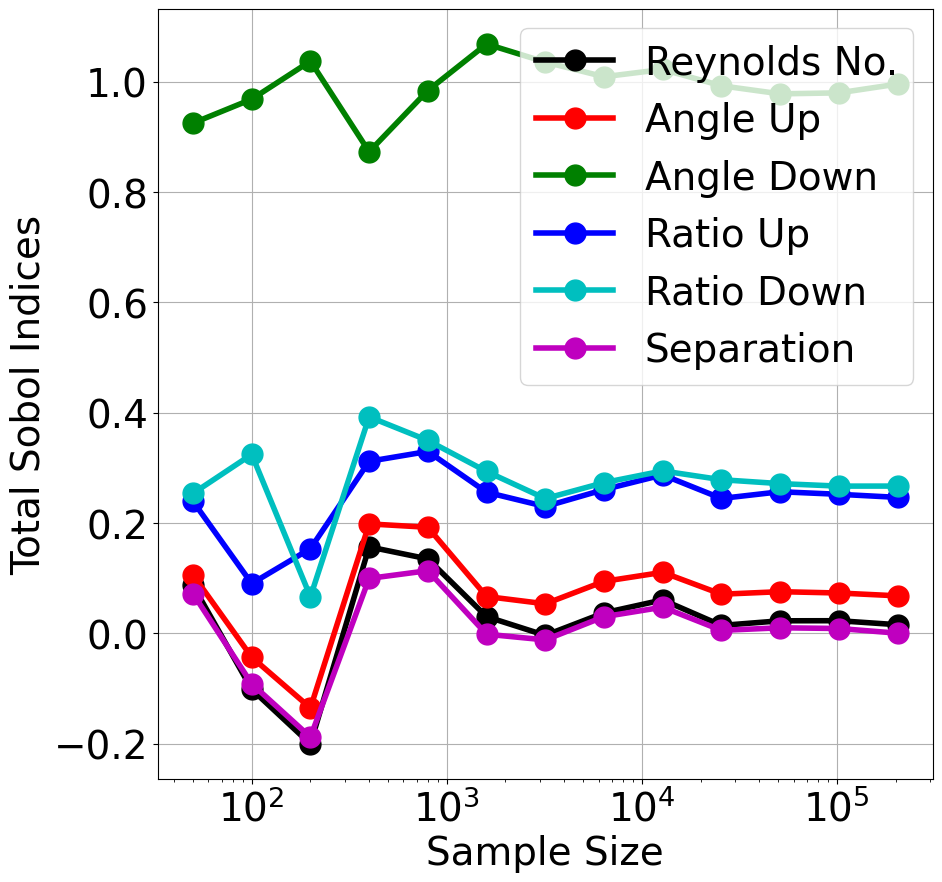
(c) Downstream Lift Coefficient

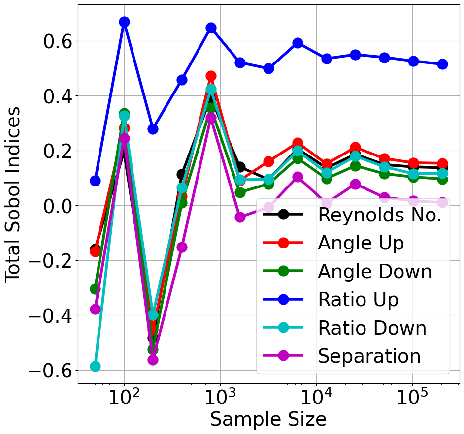
(d) Downstream Drag Coefficient

Figure 18: Case of Double Elliptic Cylinder: Estimation of Total Sobol Indices: Convergence of Monte-Carlo Method

For the case of double cylinders, there are 4 outputs and 6 inputs as shown in fig. 4(b). Hence, there are $6\times 4=24$ total Sobol indices. Figure 18 plots the convergence for increase in sample size by a factor of 2 starting from 50. The stationarity is reached beyond 1E4 samples. Average of last five samples is recorded as the converged estimate in fig. 19. Similar to the case of single cylinder, the lift coefficients of both the cylinders are highly sensitive to their respective angles of attack. The lift and drag of the upstream cylinder are not sensitive to the parameters of the downstream cylinder. This shows that the downstream cylinder has negligible effect on the upstream cylinder. Moreover, these sensitivity indices in fig. 19(a) are fairly close to the indices of single cylinder in fig. 17. On the other hand the downstream cylinder is affected significantly by the upstream cylinder. Thus, the downstream drag is most sensitive to the upstream ratio. Hence, the Sobol indices give insight in the system and highlight the underlying physics. The input parameters with higher indices should be tightly controlled since their stochastic variation affects the output significantly. Those inputs with lower indices can be loosely controlled as their impact on the output is minimal. This information can be used practically during the design and manufacturing stages.

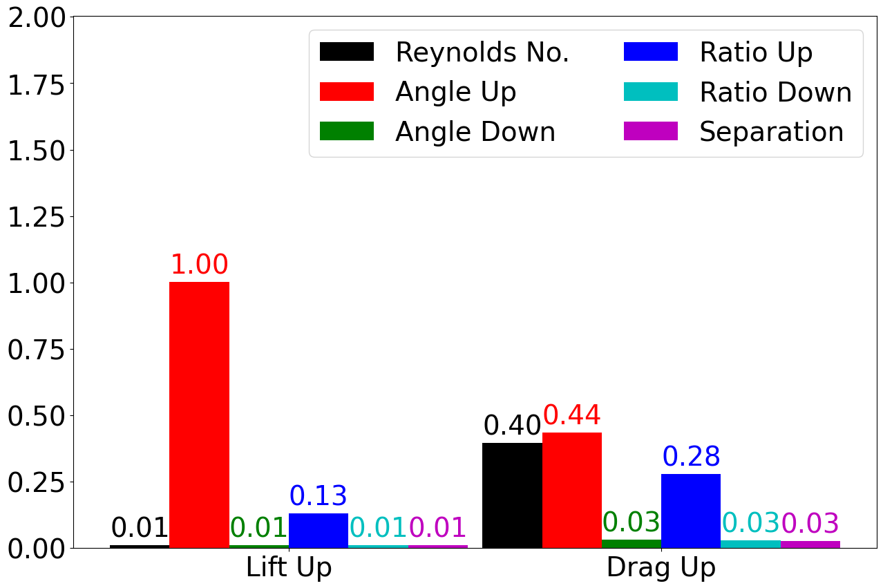
(a) Upstream Lift and Drag

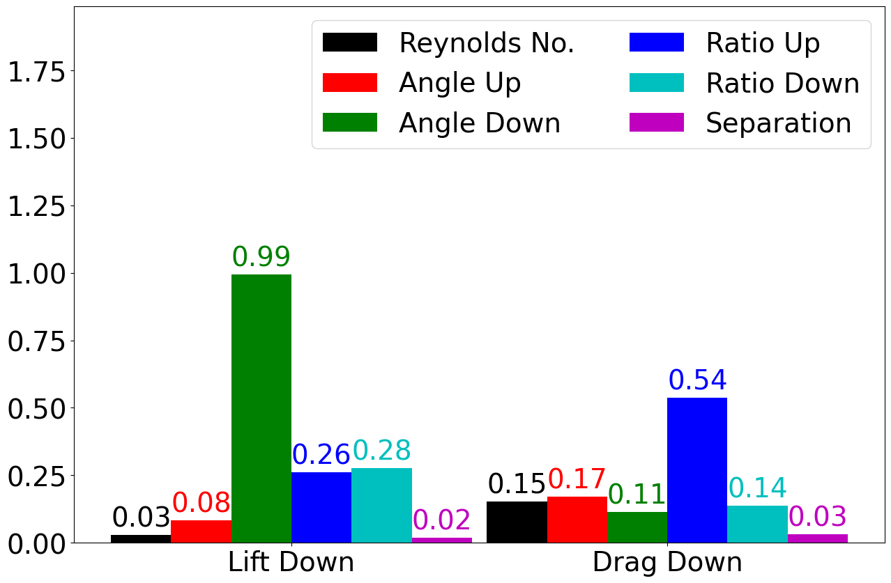
(b) Downstream Lift and Drag

Figure 19: Case of Double Elliptic Cylinder: Total Sobol Indices: Sensitivity of Lift and Drag to 6 Inputs

6 Summary and Future Work

In the present paper, we have trained multilayer perceptron neural networks (MLPNN) for prediction of lift and drag coefficients due to flow over single and tandem elliptic cylinders of arbitrary aspect ratios, angles of attack, inter-cylinder distance and flow Reynolds number. First, a large set of CFD simulations are conducted using the COMSOL Multiphysics computer program for parameters selected on a three (or six) dimensional Latin hypercube. The calculations store the coefficients of lift and drag which are used to train the MLPNNs. After training, the networks are validated against separate unseen data sets, and good agreement is observed. The parametric variation of the lift and drag coefficients for a single cylinder are presented for different Reynolds numbers, angle of attack, and aspect ratio of the cylinder.

A detailed sensitivity analysis is carried out using the MLPNN for lift and drag. The data sample for the sensitivity studies using the Monte-Carlo method is generated by the neural networks. The sample size is increased exponentially until the sensitivity coefficient converges to a value independent of the sample size. It can be seen that using the neural network as a surrogate model is essential since running a hundred thousand numerical simulations is computationally expensive. The study indicates which parameters are most influential over others in impacting the output variables. For a single cylinder, the lift coefficient is strongly dependent on the angle of attack, while the drag is a strong function of the Reynolds number. For the case of tandem cylinders, the lift on the upstream cylinder is most sensitive to its angle of attack, while drag is equally sensitive to the Reynolds number and upstream angle of attack. The lift on the downstream cylinder is a strong function of the angle of attack of the upstream cylinder, while the drag on the downstream cylinder is most sensitive to the upstream cylinder aspect ratio.

The current study has been limited to the steady region. Efforts are underway to consider supercritical Reynolds number for which the flow will become unsteady with periodic shedding of vortices.

References

- Goodfellow et al. [2016] I. Goodfellow, Y. Bengio, A. Courville, Deep Learning, MIT Press, 2016. http://www.deeplearningbook.org.
- Peng et al. [2020] G. C. Peng, M. Alber, A. B. Tepole, W. R. Cannon, S. De, S. Dura-Bernal, K. Garikipati, G. Karniadakis, W. W. Lytton, P. Perdikaris, et al., Multiscale modeling meets machine learning: What can we learn?, Archives of Computational Methods in Engineering (2020) 1–21.
- Schmidhuber [2015] J. Schmidhuber, Deep learning in neural networks: An overview, Neural networks 61 (2015) 85–117.
- McKay et al. [2000] M. D. McKay, R. J. Beckman, W. J. Conover, A comparison of three methods for selecting values of input variables in the analysis of output from a computer code, Technometrics 42 (2000) 55–61.
- Iman et al. [1981] R. L. Iman, J. C. Helton, J. E. Campbell, An approach to sensitivity analysis of computer models: Part i—introduction, input variable selection and preliminary variable assessment, Journal of quality technology 13 (1981) 174–183.
- Han et al. [2019] R. Han, Y. Wang, Y. Zhang, G. Chen, A novel spatial-temporal prediction method for unsteady wake flows based on hybrid deep neural network, Physics of Fluids 31 (2019) 127101.
- Miyanawala and Jaiman [2017] T. Miyanawala, R. Jaiman, An efficient deep learning technique for the navier-stokes equations: Application to unsteady wake flow dynamics, arXiv preprint arXiv:1710.09099 (2017).
- Bukka et al. [2020] S. Bukka, R. Gupta, A. Magee, R. Jaiman, Assessment of unsteady flow predictions using hybrid deep learning based reduced order models, arXiv preprint arXiv:2009.04396 (2020).
- Ribeiro et al. [2020] M. Ribeiro, A. Rehman, S. Ahmed, A. Dengel, Deepcfd: Efficient steady-state laminar flow approximation with deep convolutional neural networks, arXiv preprint arXiv:2004.08826 (2020).
- Sekar et al. [2019] V. Sekar, Q. Jiang, C. Shu, B. Khoo, Fast flow field prediction over airfoils using deep learning approach, Physics of Fluids 31 (2019) 057103.
- Raissi and Karniadakis [2018] M. Raissi, G. Karniadakis, Hidden physics models: Machine learning of nonlinear partial differential equations, Journal of Computational Physics 357 (2018) 125–141.
- Ogoke et al. [2020] F. Ogoke, K. Meidani, A. Hashemi, A. B. Farimani, Graph convolutional neural networks for body force prediction, arXiv preprint arXiv:2012.02232 (2020).
- Jin et al. [2018] X. Jin, P. Cheng, W. Chen, H. Li, Prediction model of velocity field around circular cylinder over various reynolds numbers by fusion convolutional neural networks based on pressure on the cylinder, Physics of Fluids 30 (2018) 047105.
- Deng et al. [2019] Z. Deng, C. He, Y. Liu, K. Kim, Super-resolution reconstruction of turbulent velocity fields using a generative adversarial network-based artificial intelligence framework, Physics of Fluids 31 (2019) 125111.
- Sang et al. [2021] J. Sang, X. Pan, T. Lin, W. Liang, G. Liu, A data-driven artificial neural network model for predicting wind load of buildings using gsm-cfd solver, European Journal of Mechanics-B/Fluids 87 (2021) 24–36.
- Seo et al. [2020] Y. M. Seo, K. Luo, M. Y. Ha, Y. G. Park, Direct numerical simulation and artificial neural network modeling of heat transfer characteristics on natural convection with a sinusoidal cylinder in a long rectangular enclosure, International Journal of Heat and Mass Transfer 152 (2020) 119564.
- Seo et al. [2021] Y. M. Seo, S. Pandey, H. U. Lee, C. Choi, Y. G. Park, M. Y. Ha, Prediction of heat transfer distribution induced by the variation in vertical location of circular cylinder on rayleigh-bénard convection using artificial neural network, International Journal of Mechanical Sciences 209 (2021) 106701.
- Zhang et al. [2019] M. Zhang, Z. Zheng, Y. Liu, X. Jiang, Numerical simulation and neural network study using an upstream cylinder for flow control of an airfoil, in: Fluids Engineering Division Summer Meeting, volume 59032, American Society of Mechanical Engineers, 2019, p. V002T02A045.
- Alizadeh et al. [2020] R. Alizadeh, J. Mohebbi Najm Abad, A. Fattahi, E. Alhajri, N. Karimi, Application of machine learning to investigation of heat and mass transfer over a cylinder surrounded by porous media—the radial basic function network, Journal of Energy Resources Technology 142 (2020) 112109.
- Tang et al. [2020] H. Tang, J. Rabault, A. Kuhnle, Y. Wang, T. Wang, Robust active flow control over a range of reynolds numbers using an artificial neural network trained through deep reinforcement learning, Physics of Fluids 32 (2020) 053605.
- Shahane et al. [2020] S. Shahane, N. Aluru, P. Ferreira, S. G. Kapoor, S. P. Vanka, Optimization of solidification in die casting using numerical simulations and machine learning, Journal of Manufacturing Processes 51 (2020) 130–141.
- Zhang et al. [2019] D. Zhang, L. Lu, L. Guo, G. E. Karniadakis, Quantifying total uncertainty in physics-informed neural networks for solving forward and inverse stochastic problems, Journal of Computational Physics 397 (2019) 108850.
- Shahane et al. [2019] S. Shahane, N. R. Aluru, S. P. Vanka, Uncertainty quantification in three dimensional natural convection using polynomial chaos expansion and deep neural networks, International Journal of Heat and Mass Transfer 139 (2019) 613–631.
- Braza et al. [1986] M. Braza, P. Chassaing, H. H. Minh, Numerical study and physical analysis of the pressure and velocity fields in the near wake of a circular cylinder, Journal of fluid mechanics 165 (1986) 79–130.
- Williamson [1996] C. H. Williamson, Vortex dynamics in the cylinder wake, Annual review of fluid mechanics 28 (1996) 477–539.
- Dennis and Chang [1970] S. Dennis, G.-Z. Chang, Numerical solutions for steady flow past a circular cylinder at reynolds numbers up to 100, Journal of Fluid Mechanics 42 (1970) 471–489.
- Tritton [1959] D. J. Tritton, Experiments on the flow past a circular cylinder at low reynolds numbers, Journal of Fluid Mechanics 6 (1959) 547–567.
- Zdravkovich [1997] M. Zdravkovich, Flow around circular cylinders; vol. i fundamentals, Journal of Fluid Mechanics 350 (1997) 377–378.
- Shahane et al. [2021] S. Shahane, A. Radhakrishnan, S. P. Vanka, A high-order accurate meshless method for solution of incompressible fluid flow problems, Journal of Computational Physics 445 (2021) 110623.
- Shahane and Vanka [2021] S. Shahane, S. P. Vanka, A semi-implicit meshless method for incompressible flows in complex geometries, arXiv preprint arXiv:2106.07616 (2021).
- Okajima [1982] A. Okajima, Strouhal numbers of rectangular cylinders, Journal of Fluid mechanics 123 (1982) 379–398.
- Sharma and Eswaran [2004] A. Sharma, V. Eswaran, Heat and fluid flow across a square cylinder in the two-dimensional laminar flow regime, Numerical Heat Transfer, Part A: Applications 45 (2004) 247–269.
- Jackson [1987] C. Jackson, A finite-element study of the onset of vortex shedding in flow past variously shaped bodies, Journal of fluid Mechanics 182 (1987) 23–45.
- Robichaux et al. [1999] J. Robichaux, S. Balachandar, S. P. Vanka, Three-dimensional floquet instability of the wake of square cylinder, Physics of Fluids 11 (1999) 560–578.
- Mukhopadhyay et al. [1992] A. Mukhopadhyay, G. Biswas, T. Sundararajan, Numerical investigation of confined wakes behind a square cylinder in a channel, International journal for numerical methods in fluids 14 (1992) 1473–1484.
- Najjar and Vanka [1995] F. M. Najjar, S. Vanka, Simulations of the unsteady separated flow past a normal flat plate, International journal for numerical methods in fluids 21 (1995) 525–547.
- Dennis and Dunwoody [1966] S. Dennis, J. Dunwoody, The steady flow of a viscous fluid past a flat plate, Journal of Fluid Mechanics 24 (1966) 577–595.
- Saha [2007] A. K. Saha, Far-wake characteristics of two-dimensional flow past a normal flat plate, Physics of Fluids 19 (2007) 128110.
- Kemp [2019] M. Kemp, Leonardo da vinci’s laboratory: studies in flow, Nature 571 (2019) 322–324.
- Shintani et al. [1983] K. Shintani, A. Umemura, A. Takano, Low-reynolds-number flow past an elliptic cylinder, Journal of Fluid Mechanics 136 (1983) 277–289.
- Park et al. [1989] J. K. Park, S. O. Park, J. M. Hyun, Flow regimes of unsteady laminar flow past a slender elliptic cylinder at incidence, International journal of heat and fluid flow 10 (1989) 311–317.
- Raman et al. [2013] S. K. Raman, K. Arul Prakash, S. Vengadesan, Effect of axis ratio on fluid flow around an elliptic cylinder—a numerical study, Journal of fluids engineering 135 (2013).
- Paul et al. [2014] I. Paul, K. A. Prakash, S. Vengadesan, Numerical analysis of laminar fluid flow characteristics past an elliptic cylinder, International Journal of Numerical Methods for Heat & Fluid Flow (2014).
- Lugt and Haussling [1974] H. Lugt, H. Haussling, Laminar flow past an abruptly accelerated elliptic cylinder at 45 incidence, Journal of Fluid Mechanics 65 (1974) 711–734.
- Taneda [1972] S. Taneda, The development of the lift of an impulsively started elliptic cylinder at incidence, Journal of the Physical Society of Japan 33 (1972) 1706–1711.
- Patel [1981] V. Patel, Flow around the impulsively started elliptic cylinder at various angles of attack, Computers & Fluids 9 (1981) 435–462.
- Ota et al. [1987] T. Ota, H. Nishiyama, Y. Taoka, Flow around an elliptic cylinder in the critical reynolds number regime (1987).
- Nair and Sengupta [1997] M. Nair, T. Sengupta, Unsteady flow past elliptic cylinders, Journal of fluids and structures 11 (1997) 555–595.
- Faruquee et al. [2007] Z. Faruquee, D. S. Ting, A. Fartaj, R. M. Barron, R. Carriveau, The effects of axis ratio on laminar fluid flow around an elliptical cylinder, International Journal of Heat and Fluid Flow 28 (2007) 1178–1189.
- Dennis and Young [2003] S. Dennis, P. Young, Steady flow past an elliptic cylinder inclined to the stream, Journal of engineering mathematics 47 (2003) 101–120.
- Badr et al. [2001] H. Badr, S. Dennis, S. Kocabiyik, Numerical simulation of the unsteady flow over an elliptic cylinder at different orientations, International journal for numerical methods in fluids 37 (2001) 905–931.
- D’alessio and Dennis [1995] S. D’alessio, S. Dennis, Steady laminar forced convection from an elliptic cylinder, Journal of engineering mathematics 29 (1995) 181–193.
- D’alessio et al. [1999] S. D’alessio, S. Dennis, P. Nguyen, Unsteady viscous flow past an impulsively started oscillating and translating elliptic cylinder, Journal of engineering mathematics 35 (1999) 339–357.
- Ota and Nishiyama [1986] T. Ota, H. Nishiyama, Flow around two elliptic cylinders in tandem arrangement (1986).
- Shahane [2019] S. Shahane, Numerical simulations of die casting with uncertainty quantification and optimization using neural networks, Ph.D. thesis, University of Illinois at Urbana-Champaign, 2019.
- Abadi et al. [2015] M. Abadi, A. Agarwal, P. Barham, E. Brevdo, Z. Chen, C. Citro, G. Corrado, A. Davis, J. Dean, M. Devin, S. Ghemawat, I. Goodfellow, A. Harp, G. Irving, M. Isard, Y. Jia, R. Jozefowicz, L. Kaiser, M. Kudlur, J. Levenberg, D. Mané, R. Monga, S. Moore, D. Murray, C. Olah, M. Schuster, J. Shlens, B. Steiner, I. Sutskever, K. Talwar, P. Tucker, V. Vanhoucke, V. Vasudevan, F. Viégas, O. Vinyals, P. Warden, M. Wattenberg, M. Wicke, Y. Yu, X. Zheng, TensorFlow: Large-scale machine learning on heterogeneous systems, 2015. URL: https://www.tensorflow.org/, software available from tensorflow.org.
- Chollet et al. [2015] F. Chollet, et al., Keras, https://keras.io, 2015.
- Kingma and Ba [2014] D. P. Kingma, J. Ba, Adam: A method for stochastic optimization, arXiv preprint arXiv:1412.6980 (2014).
- Cameron and Windmeijer [1997] A. C. Cameron, F. A. Windmeijer, An r-squared measure of goodness of fit for some common nonlinear regression models, Journal of econometrics 77 (1997) 329–342.
- Sobol [2001] I. M. Sobol, Global sensitivity indices for nonlinear mathematical models and their monte carlo estimates, Mathematics and computers in simulation 55 (2001) 271–280.
- Saltelli et al. [2008] A. Saltelli, M. Ratto, T. Andres, F. Campolongo, J. Cariboni, D. Gatelli, M. Saisana, S. Tarantola, Global sensitivity analysis: the primer, John Wiley & Sons, 2008.
- Caflisch [1998] R. Caflisch, Monte carlo and quasi-monte carlo methods, Acta Numerica 7 (1998) 1–49.