From the Lagrange polygon to the figure eight I

Abstract

The present work studies the continuation class of the regular $n$-gon solution of the $n$-body problem. For odd numbers of bodies between $n=3$ and $n=15$ we apply one parameter numerical continuation algorithms to the energy/frequency variable, and find that the figure eight choreography can be reached starting from the regular $n$-gon. The continuation leaves the plane of the $n$-gon, and passes through families of spatial choreographies with the topology of torus knots. Numerical continuation out of the $n$-gon solution is complicated by the fact that the kernel of the linearization there is high dimensional. Our work exploits a symmetrized version of the problem which admits dense sets of choreography solutions, and which can be written as a delay differential equation in terms of one of the bodies. This symmetrized setup simplifies the problem in several ways. On one hand, the direction of the kernel is determined automatically by the symmetry. On the other hand, the set of possible bifurcations is reduced and the $n$-gon continues to the eight after a single symmetry breaking bifurcation. Based on the calculations presented here we conjecture that the $n$-gon and the eight are in the same continuation class for all odd numbers of bodies.

1 Introduction

The qualitative theory of nonlinear dynamics has deep roots in the pioneering work of Poincaré MR926906 ; MR926907 ; MR926908 , where invariant sets – and periodic orbits in particular – play a central organizational role. Inspired by the work of Poincaré, a number of late Nineteenth and early Twentieth Century astronomers like Darwin, Moulton, and Strömgren conducted thorough numerical studies of periodic motions in gravitational $n$–body problems long before the advent of digital computing MR1554890 ; MR0094486 ; Stromgren . Over the last century scientific interest in $n$-body dynamics has only increased, driving developments in diverse fields from computational mathematics to algebraic topology. By now the literature is rich enough to discourage even a terse survey. We refer to the Lecture notes of Chenciner MR3329413 , as well as the books of Moser, Meyer and Hall, and Szebehely MR1829194 ; MR2468466 ; theoryOfOrbits where the interested reader will find both modern overviews of the theory and thorough reviews of the literature.

The present work is concerned with a special class of periodic orbits known as choreographies, where $n$ gravitating bodies follow one another around the same closed curve in $\mathbb{R}^{3}$. The most basic example of a choreography comes from the classical equilateral triangle configuration of Lagrange, where three massive bodies are located at the vertices of a rigid equilateral triangle revolving around the center of mass. If the bodies all have the same mass then each goes around the same circle with constant angular velocity. This is an example of a circular choreography. See the left frame of Figure 1.

Lagrange published this special solution of the three body problem in 1772 lagrangeTriangle . The result was generalized by Hoppe in 1879 nGonPaper , giving the existence of a circular choreography for any number of bodies. In this case the bodies are arranged at the vertices of a rotating regular $n$-gon, and the choreography is the inscribing circle. In 1985 Perko and Walter PerkoW85 showed that when $n\geq 4$, in contrast to the 3 body case, the $n$-gon solution exists if and only if the masses of the $n$ bodies are equal. The right frame of Figure 1 illustrates a circular $n$-gon choreography solution for the case of $n=15$ bodies.

The first non-circular choreography solution was discovered numerically by C. Moore in the early 1990’s Mo93 . This solution consists of three bodies of equal mass following one another around the now famous figure-eight orbit. See the left frame of Figure 2. Chenciner and Montgomery, in ChMo00 gave a rigorous mathematical proof of the existence of the figure-eight choreography by minimizing the Newtonian action functional over paths connecting collinear and isosceles configurations of the three bodies. Many additional numerical results for the eight are described by Simó in MR1884902 , who also coined the term choreography. Several animations of $n$-body choreographies are found at the webpage renatoAnimations .

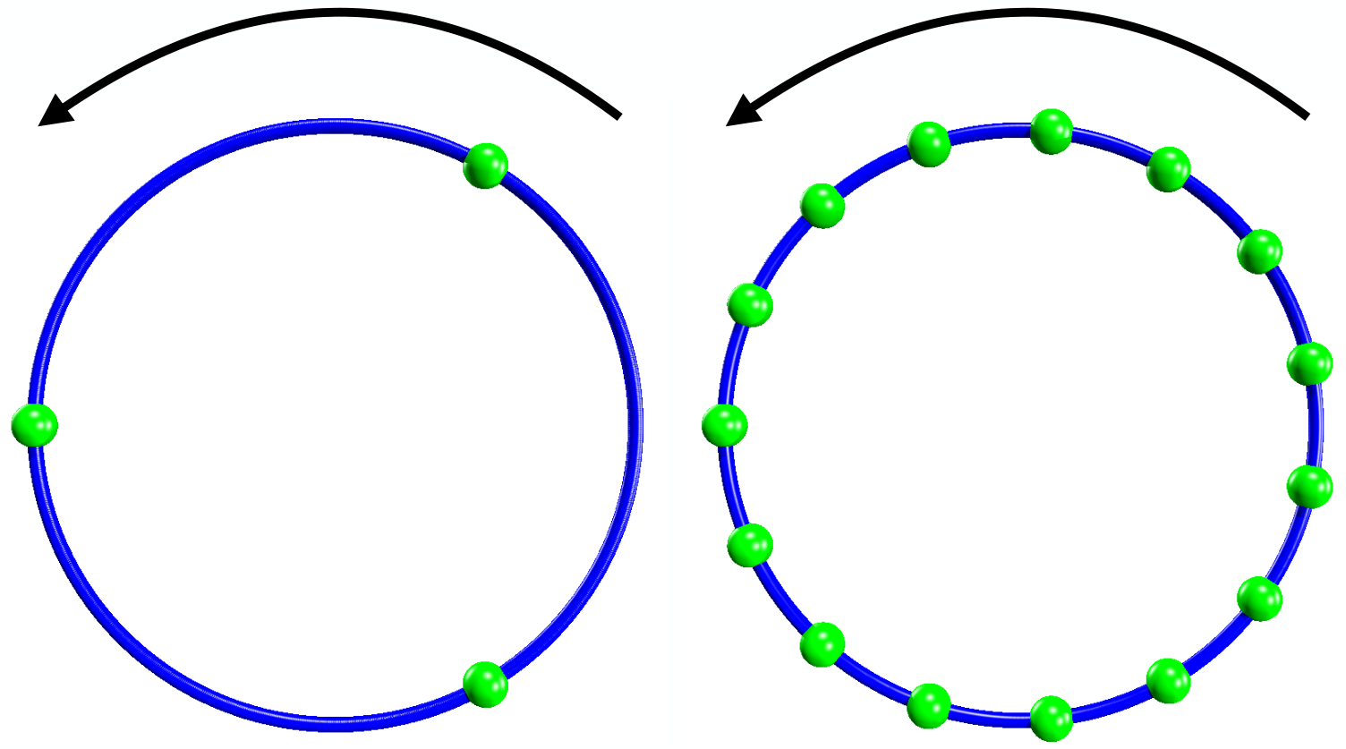
Figure 1: Circular Choreographies: In this figure green spheres represent masses and the blue curve illustrates the circular choreography followed by the bodies. The left frame illustrates a “snap shot” of the equilateral triangle solution of Lagrange. At each instant the three bodies are located at the vertices of an equilateral triangle, which rigidly rotates with constant angular velocity. When the masses are equal the triangle revolves about the center of mass of the three bodies. The right frame illustrates a 15 body circular choreography, where at each moment the bodies are located at the vertices of a regular $15$-gon. The snapshot rotates the center of mass with constant angular velocity. Note that if we change to co-rotating coordinates (rotating coordinate frame origin at the center of mass and angular velocity matching the angular velocity of the triangle/polygon) then the triangle/polygon represents an equilibrium configuration in rotating coordinates.

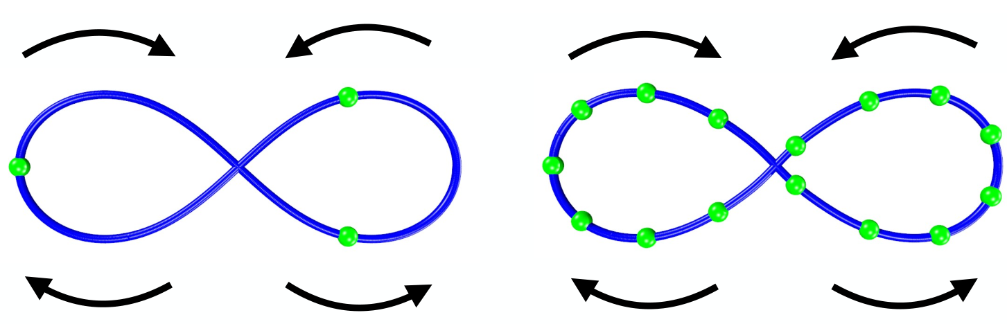
Figure 2: Figure Eight Choreographies: just as in Figure 1, green spheres represent the massive bodies and the blue curve illustrates the path of the choreography orbit. The left frame illustrates a “snap shot” of the three body eight, and the arrows indicate the motion along the various segments of the curve. The right frame is similar, illustrating a 15 body eight.

It is a fundamental geometric property of conservative systems that periodic orbits occur in one parameter families, or tubes, smoothly parameterized by energy/frequency. We say that two periodic orbits are in the same continuation class if one can be reached from the other by continuous variation of the energy. Note that, because of bifurcations, the global geometry of a continuation class is not a single tube but rather a “tree”, possibly with many branches.

The literature discussed in the preceding paragraphs makes it clear that the three body problem admits at least two distinct choreography solutions: the equilateral triangle and the eight. Moreover, the symmetry group of the eight choreography is a $12^{th}$-order subgroup of the symmetry group of the equilateral triangle. Then a natural question is: are these co-existing choreographies are related by continuation? Indeed, one finds in the $2010$ Mémoire D’Habilitation of Jacques Féjoz fijozHabilatation the following recollection regarding Christian Marchal: that “in 1999, when he (Marchal) heard about the choreographic figure-eight solution of Chenciner-Montgomery, he at once imagined that the eight could be the unknown end of $P12$.” Here $P12$ is an out of plane family of periodic orbits related to the equilateral triangle of Lagrange and discussed in somewhat more detail below. These remarks are formalized as follows.

Conjecture 1 (Marchal’s Conjecture)

The three body equilateral triangle of Lagrange and the three body figure eight are in the same continuation class.

The conjecture appeared also in the 2005 paper of Chenciner, Féjoz, and Montgomery. See also the lecture notes of Chenciner MR2446248 . Careful numerical calculations supporting Marchal’s conjecture are found in the $2008$ work of Wulff and Schebesch MR2429679 on numerical continuation of relative periodic orbits in Hamiltonian systems.

We remark that Conjecture 1 should be regarded as something much more than a mathematical curiosity. In the precise sense of global bifurcation theory, the conjecture concerns the question where does the figure eight choreography come from? We hasten to add that, to the best of our knowledge, the conjecture remains unproved in a completely mathematically rigorous sense. Indeed, as is discussed further in fijozHabilatation , it appears to be very difficult to obtain the estimates necessary for a variational proof of Conjecture 1.

We now describe in somewhat more detail the $P12$ vertical family of periodic orbits already alluded to above. The three body equilateral triangle configuration of Lagrange corresponds to an equilibrium solution of the rotating three body problem, and the existence of an attached family of vertical Lyapunov periodic orbits is established by Chenciner and Féjoz in ChFe07 . The authors of ChFe07 compute a normal form at the Lagrange relative equilibrium and deduce that there is a unique (up to symmetries) bifurcating spatial family: the so called $P12$ family. The family is important because, as long as it varies continuously with respect to the frequency parameter, it provides –upon returning to the inertial frame– a dense set of choreographic solutions to the three body problem. Continuity with respect to frequency was further established in ChFe08 for frequencies close to the Lagrange triangle.

Using an approach based on equivariant bifurcation theory, García-Azpeitia and Ize in GaIz11 ; GaIz13 studied in rotating coordinates the global existence of the vertical Lyapunov family arising from the Lagrange triangle. The term global means here that the family forms a continuum (“tube”) in an appropriate Sobolev space of normalized $2\pi$ periodic solutions. The continuum is parameterized by frequency and terminates in one of the following alternatives: the Sobolev norm of the orbits in the family tends to infinity, the period of the orbits tends to infinity, the family ends in an orbit with collision, or the family returns to another equilibrium solution. Without additional information it is not possible to know which alternative actually occurs, but this vertical Lyapunov family makes a good candidate for exploring the continuation from the equilateral triangle to the eight because of the fact that it gives rise to choreography solutions.

What is more, the geometric picture just described extends naturally to any odd number of bodies. The regular $n$-gon solution of Hoppe nGonPaper (mentioned above) provides a circular choreography, and hence a relative equilibrium solution in rotating coordinates, for any number of bodies. The $n$-gon equilibrium in the rotating $n$-body problem has always an attached vertical family of Lyapunov periodic orbits GaIz11 ; GaIz13 . For any even number of bodies the existence of a figure eight choreography can be ruled out via symmetry considerations (it would result in a finite time collision). Yet for an odd numbers of bodies it is physically possible to have a figure eight, and indeed one finds numerical evidence supporting the existence of $5$ and $19$ body eights in the classic work of Simó Si00 . See also Ferrario and Terracini FeTe04 , and note that the right frame of Figure 2 illustrates a numerically computed 15-body eight. Then one can ask: for which odd numbers $n$ are the $n$-gon and $n$-body eight in the same continuation family?

The study by Calleja, Doedel, and García-Azpeitia CaDoGa18 casts additional light on the question. In that reference the authors explore the behavior of the vertical family for different numbers of bodies using numerical continuation methods. Of particular importance to the present study, the authors of CaDoGa18 discovered a numerical continuation leading from the $7$-gon to the $7$-body eight. The continuation passes through the vertical Lyapunov (or $P12$) family, but also involves a symmetry breaking bifurcation from this family. The occurrence of bifurcations helps to explain the difficulty in applying variational methods.

Combining the three body numerical continuations from MR2429679 with the five body numerical continuations from CaDoGa18 an interesting picture begins to emerge. These studies suggest the possibility that, for odd numbers of bodies, continuation from the $n$-gon to the eight may be the rule rather than the exception. This question motivates the present work.

We exploit the functional analytic framework for studying $n$-body choreographies put forward by the authors of the present study in the recent work ourTorusKnots . Our approach explicitly incorporates the symmetries and reduces the $n$-body choreography problem to a system of six scalar delay differential equations (DDE) describing the location of one of the bodies. The idea is that $n$-bodies on a choreography swap locations with one another after a fixed fraction of the period, so that the gravitational force exerted by body $j$ on body $k$ can be rewritten in terms of a force exerted on body $k$ by itself after an appropriate time shift – hence the delay. Under explicit number theoretic conditions on the frequency, periodic solutions of the rotating DDE provide choreography orbits of the Newtonian $n$-body problem back in the inertial reference frame.

Another notable component of the present work is that we incorporate the theoretical insights GaIz11 ; GaIz13 into our numerical continuation framework. More precisely, we exploit the first order description of the vertical Lyapunov family given in the reference just cited to “find our way out” of the high dimensional kernel caused by the high order resonances at the triangle. In fact the results of GaIz11 ; GaIz13 apply to any number of bodies at relative equilibrium on the $n$-gon. This leads to a general numerical procedure for starting the continuation of the vertical Lyapunov family for any number of bodies, and allows us to explore the continuation branch in an automatic fashion. The numerical explorations to be presented in the remainder of the present work suggest the following conjecture.

Conjecture 2 (Generalized Marchal’s Conjecture)

For any odd number of bodies, the $n$-gon choreography and the $n$-body figure eight are in the same continuation class.

We present numerical continuation results for every odd number of bodies from $n=3$ to $n=15$, as evidence in support of the conjecture. Again, the three and fifteen body eights at the end of the continuation are illustrated in Figure 2. It is also very interesting to report that in each case the qualitative features of the continuation are the same. In the symmetrized version of the problem, the $n$-body figure eight occurs always after a single axial bifurcation from the vertical Lyapunov family associated with the regular $n$-gon.

Remark 1 (DDEs versus ODEs)

In one sense passing to a system of DDEs provides a dramatic reduction in the dimension of the problem, as we obtain a six scalar equations describing a single body instead of a system $6n$ scalar equations for all $n$ bodies. On the other hand, the appearance of delays in the problem could be viewed as a major technical disadvantage. This is because initial value problems for DDEs lead to infinite dimensional complications, while the $n$-body problem is inherently finite dimensional. Nevertheless, after restricting ones attention to periodic solutions and projecting into Fourier space, both the delay and the differential operators are reduced to diagonal operations in the space of complex Fourier coefficients. Thanks to this observation it is the case that, after projecting to Fourier space, studying a periodic orbit of a system of $6$ DDEs is in principle no more difficult than studying a periodic orbit in a system of $6$ ODEs. Moreover, explicitly incorporating the choreographic symmetries into the problem results in fewer bifurcations along the periodic branch than would be encountered if we continued the vertical family in the full rotating $n$-body problem. To put it another way, in the $n$-body problem a periodic orbit bifurcating from a choreography need not be a choreography. While in the DDE, we only see bifurcations that result in new branches containing dense sets of choreographies.

The remainder of the paper is organized as follows. In Section 2, we review the functional analytic formulation of the $n$-body choreography problem developed in ourTorusKnots . In Section 3 we discuss the results of a number of numerical continuations, where we examine (in Section 3.3) the stability of the orbits. Finally, in Section 4 we discuss the prospects for applying computer-assisted methods of proof to the generalized conjecture for finite numbers of bodies.

2 Functional analytic formulation of the $n$-body choreography problem

We describe the movement of the $n$ bodies in a rotating frame with frequency $\sqrt{s_{1}}$, where

$$s_{1}\,\stackrel{{\scriptstyle\mbox{\tiny{\raisebox{0.0pt}[0.0pt][0.0pt]{def}}}}}{{=}}\,\frac{1}{4}\sum_{j=1}^{n-1}\frac{1}{\sin(j\zeta/2)},\qquad\zeta\,\stackrel{{\scriptstyle\mbox{\tiny{\raisebox{0.0pt}[0.0pt][0.0pt]{def}}}}}{{=}}\,\frac{2\pi}{n}.$$ (1)

We assume that the masses of the $n$ bodies are equal to $1$. Thus the $2\pi/\omega$-periodic solutions of the $n$-body problem in the rotating frame are solutions in the inertial frame of the form

$$q_{j}(t)=e^{\sqrt{s_{1}}t\bar{J}}u_{j}(\omega t),\qquad j=1,\dots,n$$

where $u_{j}(t)$ are $2\pi$-periodic functions and $\bar{J}=J\oplus 0$ with $J$ the usual symplectic matrix in $\mathbb{R}^{2}$. Therefore Newton equations in the coordinates $u_{j}$ read as

$$\left(\omega\partial_{t}+\sqrt{s_{1}}\bar{J}\right)^{2}u_{j}=\nabla_{u_{j}}U=-\sum_{i=1(i\neq j)}^{n}\frac{u_{j}-u_{i}}{\left\|u_{j}-u_{i}\right\|^{3}},$$ (2)

where $U$ is the potential energy

$$U=\sum_{i<j}\frac{1}{\left\|u_{j}-u_{i}\right\|}.$$

Actually, the frequency of rotation is chosen to be$\sqrt{s_{1}}$ such that the $n$-polygon comprised of $n$ bodies on the unit circle, $a_{j}\,\stackrel{{\scriptstyle\mbox{\tiny{\raisebox{0.0pt}[0.0pt][0.0pt]{def}}}}}{{=}}\,(\cos j\zeta,\sin j\zeta,0)$ for $j=1,...,n$, is an equilibrium solution of equations (2), for instance see GaIz11 .

Set $u=(u_{1},...,u_{n}),$ $a=(a_{1},...,a_{n})$ and $\mathcal{\bar{J}}\,\stackrel{{\scriptstyle\mbox{\tiny{\raisebox{0.0pt}[0.0pt][0.0pt]{def}}}}}{{=}}\,\bar{J}\oplus...\oplus\bar{J}.$ The linearization of the equation (2) at the polygonal equilibrium $a$ is

$$\left(\omega\partial_{t}+\sqrt{s_{1}}\mathcal{\bar{J}}\right)^{2}u=D^{2}U(a)u.$$ (3)

As a particular consequence of the results obtained in GaIz13 , we have that $u(t)=\emph{Re\,(}e^{it}w_{k})$ is a periodic solution of the linearized system (3) with frequency $\omega=\sqrt{s_{k}}$ for $k=1,...,n-1$, where

$$s_{k}\,\stackrel{{\scriptstyle\mbox{\tiny{\raisebox{0.0pt}[0.0pt][0.0pt]{def}}}}}{{=}}\,\frac{1}{4}\sum_{j=1}^{n-1}\frac{\sin^{2}(kj\zeta/2)}{\sin^{3}(j\zeta/2)}$$

and $w_{k}\,\stackrel{{\scriptstyle\mbox{\tiny{\raisebox{0.0pt}[0.0pt][0.0pt]{def}}}}}{{=}}\,\left(w_{k}^{1},...,w_{k}^{n}\right)$ is a complex vector with components $w_{k}^{j}=(0,0,e^{j(ik\zeta)})$. This implies that the linearized system at the polygon (3) has periodic solutions with frequency $\sqrt{s_{k}}$. However, since $s_{k}=s_{n-k}$ for $k\in[1,n/2)\cap\mathbb{N}$, then the set of solutions with the frequency $\omega=\sqrt{s_{k}}$ are in $1:1$ resonance. Furthermore, for the case $\omega=\sqrt{s_{1}}$ there are extra resonances with other frequencies corresponding to planar components, see GaIz13 and ChFe08 for details.

In ChFe08 , it is proven that there are families of periodic solutions that persist near the polygonal equilibrium for the $1:1$ resonance frequencies $\omega=\sqrt{s_{k}}$ using Weinstein-Moser theory. Actually, in GaIz13 it is proven that these families form a global continuous branch of solutions (vertical Lyapunov families) with symmetries

$$u_{j}(t)=e^{\ j\bar{J}\zeta}u_{n}(t+jk\zeta)\text{.}$$ (4)

The existence of a dense set of choreographies in the vertical Lyapunov families was first pointed out in ChFe08 . Later on, in CaDoGa18 was observed that if $p$ and $q$ are relatively prime such that

$$kq-p\in n\mathbb{Z},$$ (5)

an orbit in the vertical Lyapunov family with the symmetries of (4) having frequency $\omega=\sqrt{s_{1}}p/q$ is a simple choreography in the inertial reference frame. Since the set of number$\sqrt{s_{1}}p/q$ with $p$ and $q$ satisfying the diophantine equation (5) is dense, if the frequency $\omega$ varies continuously along the Lyapunov family varies, then there are infinitely many simple choreographies in the inertial frame.

Remark 2

A consequence of Proposition 3 in ourTorusKnots is that if $u_{n}(t)$ is a solution in the axial family with $p$ and $q$ satisfying (5) and its orbit does not wind around the $z$-axis, then the choreography winds on the surface of a toroidal manifold with winding numbers $p$ and $q$, i.e., the choreographic path is a $(p,q)$-torus knot. Since the figure eight is a singular $(2,1)$-torus knot, according to this principle we look for a orbit with $(p,q)=(2,1)$, i.e., our target frequency $\omega$ is

$$\omega/\sqrt{s_{1}}=2.$$

The condition (5) becomes that $k-2\in n\mathbb{Z}$. Thus the only natural match to find the $(2,1)$-torus knot (figure eight) is the branch with $k=2$. We confirm numerically that branches with $k=2$ effectively contain the figure eight choreographies.

2.1 The system reduced by symmetries

The purpose of this section is to build a self contained setting to present a systematical approach to obtain numerical computations of the periodic solutions arising from the polygonal relative equilibrium of the $n$-body problem. In a subsequent paper we plan to present rigorous validations of these families. We proceed by imposing the symmetries (4) in the system of equations (2), i.e. the system of equations is reduced to the following single equation with multiple delays for the $n$-th body

$$\mathcal{G}(u;\omega)\,\overset{\mbox{\tiny{\raisebox{0.0pt}[0.0pt][0.0pt]{def}}}}{=}\,\left(\omega\partial_{t}+\sqrt{s_{1}}\bar{J}\right)^{2}u+G(u)=0,$$ (6)

where $u(t)\in\mathbb{R}^{3}$ is the position of the $n$-th body and $G$ is the nonlinearity

$$G(u)=\sum_{j=1}^{n-1}\frac{u-e^{\ j\bar{J}\zeta}u(t+jk\zeta)}{\left\|u-e^{\ j\bar{J}\zeta}u(t+jk\zeta)\right\|^{3}}.$$

The polygonal equilibrium $a$ has the $n$-th body in the position

$$u_{0}=\left(1,0,0\right)\text{,}$$

i.e. $u_{0}$ is an equilibrium of equation (6). The linearization of $\mathcal{G}$ at $u_{0}$ is

$$D\mathcal{G}(u_{0};\omega)=\left(\omega\partial_{t}+\sqrt{s_{1}}\bar{J}\right)^{2}u+DG(u_{0}).$$

Based on the previous discussion we see that the $n$-th component of $u(t)=\emph{Im\,(}e^{it}w_{k})$, denoted by

$$u_{1}=\left(0,0,\sin t\right),$$

is in the kernel of $D\mathcal{G}(u_{0};\sqrt{s_{k}})$. Actually, to conclude that

$$D\mathcal{G}(u_{0};\sqrt{s_{k}})u_{1}=\left(s_{k}\partial_{t}^{2}+DG(u_{0})\right)u_{1}=0,$$

we only need to compute that $DG(u_{0})\,u_{1}=s_{k}u_{1}$. In the following proposition we present a self-contained proof of this fact,

Lemma 2.1

It holds that

$$DG(u_{0})\,u_{1}=s_{k}u_{1}.$$

Proof

We start by considering the nonlinear function $G(u_{0}+\sigma_{1}u_{1}^{\ast})$, where $u_{1}=Im\,u_{1}^{\ast}=(0,0,\sin t)^{T},$ and $u_{0}=(1,0,0)$ and $u_{1}^{\ast}=(0,0,e^{it})$. We compute the derivative using the formula $DG(u_{0})u_{1}=\emph{Im~{}}\left(\partial_{\sigma_{1}}G(u_{0}+\sigma_{1}u_{1}^{\ast})|_{\sigma_{1}=0}\right)$. Set

$$c=-\frac{(1-e^{ijk\zeta})^{2}}{2-2\cos(j\zeta)}=e^{ijk\zeta}\frac{\sin^{2}(jk\zeta/2)}{\sin^{2}(j\zeta/2)}\in\mathbb{C}\text{.}$$

We use the Taylor expansion

$$(1-x)^{-3/2}=1+{\frac{3}{2}}x+{\frac{15}{8}}x^{2}+{\frac{35}{16}}x^{3}+...,$$

to compute

$$\begin{split}G\left(\begin{array}[c]{c}1\\ 0\\ \sigma_{1}e^{it}\end{array}\right)&=\sum_{j=1}^{n-1}\left(\frac{1}{2^{3}\sin^{3}(j\zeta/2)\left(1-c\sigma_{1}^{2}e^{2it}\right)^{3/2}}\left(\begin{array}[c]{c}1-\cos(j\zeta)\\ -\sin(j\zeta)\\ \sigma_{1}e^{it}(1-e^{ijk\zeta})\end{array}\right)\right)\\ &=\sum_{j=1}^{n-1}\frac{1}{2^{3}\sin^{3}(j\zeta/2)}\left(1+{\frac{3}{2}}\sigma_{1}^{2}\left(ce^{2it}\right)+...\right)\left(\begin{array}[c]{c}1-\cos(j\zeta)\\ -\sin(j\zeta)\\ \sigma_{1}e^{it}(1-e^{ijk\zeta})\end{array}\right).\end{split}$$

Therefore, we have that

$$\left.\partial_{\sigma_{1}}G(u_{0}+\sigma_{1}u_{1}^{\ast})\right|_{\sigma_{1}=0}=\left(\sum_{j=1}^{n-1}\frac{1-e^{ijk\zeta}}{2^{3}\sin^{3}(j\zeta/2)}\right)\left(\begin{array}[c]{c}0\\ 0\\ e^{it}\end{array}\right).$$

Since

$$\sum_{j=1}^{n-1}\frac{1-e^{i(jk\zeta)}}{2^{3}\sin^{3}(j\zeta/2)}=\sum_{j=1}^{n-1}\frac{1-\cos kj\zeta}{2^{3}\sin^{3}(j\zeta/2)}=\frac{1}{4}\sum_{j=1}^{n-1}\frac{\sin^{2}(jk\zeta/2)}{\sin^{3}(j\zeta/2)}=s_{k}$$

we obtain that

$$DG(u_{0})\,u_{1}=\emph{Im~{}}\left(\partial_{\sigma_{1}}G(u_{0}+\sigma_{1}u_{1}^{\ast})|_{\sigma_{1}=0}\right)=s_{k}u_{1}.$$

By imposing the symmetries (4), the linear operator $D_{u}\mathcal{G}(u_{0};\sqrt{s_{k}})$ for $k\in[2,n/2]\cap\mathbb{N}$ has only half of the kernel of the $1:1$ resonance of the linearized system (3). It is important to mention that the kernel of $D\mathcal{G(}u;\sqrt{s_{k}})$ still has a high dimension; the dimension of the kernel of $D\mathcal{G(}u;\omega)$ is at least $3$ for the periodic solutions. This is due to the existence of a $3$-dimensional group of symmetries corresponding to $xy$-rotations, $z$-translations and time shift. In the following section, we use an augmented system that reduces the dimension of the kernel generated by these symmetries.

2.2 The augmented system

The problem with the kernel of $D\mathcal{G}(u_{0},\omega)$ generated by the symmetries by $xy$-rotations, $z$-translations and time shift, is solved by augmenting the map in order to isolate the orbits of solutions. In ourTorusKnots we present the augmented map that also turns the non-polynomial DDE into a higher dimensional DDE with polynomial nonlinearities.

The augmented system with polynomial nonlinearities is given by

$$f(u,v) \,\stackrel{{\scriptstyle\mbox{\tiny{\raisebox{0.0pt}[0.0pt][0.0pt]{def}}}}}{{=}}\,\partial_{t}u-v$$ (7)

$$g(\lambda,u,v,w;\omega) \,\stackrel{{\scriptstyle\mbox{\tiny{\raisebox{0.0pt}[0.0pt][0.0pt]{def}}}}}{{=}}\,\omega^{2}\partial_{t}v+2\omega\sqrt{s_{1}}\bar{J}v-s_{1}\bar{I}u+P(u,w)+\lambda_{1}\bar{J}u+\lambda_{2}v+\lambda_{3}e_{3}$$ (8)

$$h(\alpha,u,v,w) \,\stackrel{{\scriptstyle\mbox{\tiny{\raisebox{0.0pt}[0.0pt][0.0pt]{def}}}}}{{=}}\,\left\{\partial_{t}w_{j}+w_{j}^{3}\left\langle v(t)-e^{\ j\bar{J}\zeta}v(t+jk\zeta),u(t)-e^{\ j\bar{J}\zeta}u(t+jk\zeta)\right\rangle+\alpha_{j}w_{j}^{3}\right\}_{j=1}^{n-1},$$ (9)

where $w=\left\{w_{j}\right\}_{j=1}^{n-1}$, $e_{3}=(0,0,1)$ and $P$ is the polynomial nonlinearity with delays

$$P(u,w)\,\stackrel{{\scriptstyle\mbox{\tiny{\raisebox{0.0pt}[0.0pt][0.0pt]{def}}}}}{{=}}\,\sum_{j=1}^{n-1}w_{j}^{3}\left(u(t)-e^{\ j\bar{J}\zeta}u(t+jk\zeta)\right).$$ (10)

These equations are supplemented by the Poincaré sections $\eta(u)\,\stackrel{{\scriptstyle\mbox{\tiny{\raisebox{0.0pt}[0.0pt][0.0pt]{def}}}}}{{=}}\,(I_{1},I_{2},I_{3})=0$, where

$$I_{1}(u)\,\stackrel{{\scriptstyle\mbox{\tiny{\raisebox{0.0pt}[0.0pt][0.0pt]{def}}}}}{{=}}\,\int_{0}^{2\pi}u(t)\cdot\bar{J}\tilde{u}(t)~{}dt,\qquad I_{2}(u)\,\stackrel{{\scriptstyle\mbox{\tiny{\raisebox{0.0pt}[0.0pt][0.0pt]{def}}}}}{{=}}\,\int_{0}^{2\pi}u(t)\cdot\tilde{u}^{\prime}(t)~{}dt,\qquad I_{3}(u)\,\stackrel{{\scriptstyle\mbox{\tiny{\raisebox{0.0pt}[0.0pt][0.0pt]{def}}}}}{{=}}\,\int_{0}^{2\pi}u_{3}(t)~{}dt,$$

where $\tilde{u}$ is a reference function, and the initial conditions

$$\gamma(u,w)\,\stackrel{{\scriptstyle\mbox{\tiny{\raisebox{0.0pt}[0.0pt][0.0pt]{def}}}}}{{=}}\,\left\{w_{j}(0)^{2}\left\|u(0)-e^{\ j\bar{J}\zeta}u(jk\zeta)\right\|^{2}-1\right\}_{j=1}^{n-1}=0.$$

Actually, in Proposition 4 and 5 of ourTorusKnots it is proved that the solutions of $\mathcal{G}(u,\omega)=0$ are equivalent to the solution of the augmented system of equations

$$F(x;\omega)=\left(\eta,\gamma,f,g,h\right)(x;\omega)=0,\qquad x\,\stackrel{{\scriptstyle\mbox{\tiny{\raisebox{0.0pt}[0.0pt][0.0pt]{def}}}}}{{=}}\,(\lambda,\alpha,u,v,w)\text{.}$$

We set the equilibrium for the augmented system as

$$x_{0}=\left(0,0,u_{0},0,w_{0}\right),$$ (11)

where $w_{0}=\left\{w_{j,0}\right\}_{j=1}^{n-1}$ with

$$w_{j,0}=\frac{1}{\left\|(1,0,0)-(\cos j\zeta,-\sin j\zeta,0)\right\|}=\frac{1}{2\sin j\zeta/2}\text{.}$$

Using that $u_{0}$ is a steady solution of $\mathcal{G}$ it is not difficult to see that $x_{0}$ is a steady solution of the augmented system $F(x_{0};\omega)=0$ for all $\omega.$

Set

$$x_{1}\,\stackrel{{\scriptstyle\mbox{\tiny{\raisebox{0.0pt}[0.0pt][0.0pt]{def}}}}}{{=}}\,(0,0,u_{1},v_{1},0)$$ (12)

with $u_{1}=(0,0,\sin t)$ and $v_{1}=(0,0,\cos t)$. In the following proposition we prove that $x_{1}$ is the natural extension of the element of the kernel of the augmented map $F$. Notice that from the definition of $P(u,w)$ in (10), we have that,

$$\partial_{u}P(u_{0},w_{0})u_{1}= \sum_{j=1}^{n-1}w_{j,0}^{3}\left(u_{1}(t)-e^{\ j\bar{J}\zeta}u_{1}(t+jk\zeta)\right)=\sum_{j=1}^{n-1}\frac{\sin^{2}(jk\zeta/2)}{\sin^{3}(j\zeta/2)}u_{1}=DG(u_{0})u_{1}\text{.}$$ (13)

Proposition 1

It holds that

$$DF(x_{0};\sqrt{s_{k}})x_{1}=0\text{.}$$

Proof

We have that

$$DF(x_{0})x_{1}=\left(\begin{array}[]{c}\partial_{u}\eta(x_{0})u_{1}\\ \partial_{u}\gamma(x_{0})u_{1}\\ \partial_{u}f(x_{0})u_{1}+\partial_{v}f(x_{0})v_{1}\\ \partial_{u}g(x_{0})u_{1}+\partial_{v}g(x_{0})v_{1}\\ \partial_{u}h(x_{0})u_{1}+\partial_{v}h(x_{0})v_{1}\end{array}\right).$$

At the $n$-gon, we set as reference functions $\tilde{u}=u_{1}$ and $\tilde{u}^{\prime}=u_{1}^{\prime}=v_{1}$, so

$$\partial_{u}\eta(u_{0})u_{1}=\int_{0}^{2\pi}\left(u_{1}\cdot\bar{J}u_{1},u_{1}(t)\cdot v_{1}(t),\sin t\right)=0.$$

For the derivative of $\gamma$, we have,

$$\partial_{u}\gamma(x_{0})u_{1}=\left\{2w_{j,0}(0)^{2}\left\langle u_{0}(0)-e^{\ j\bar{J}\zeta}u_{0}(jk\zeta),u_{1}(0)-e^{\ j\bar{J}\zeta}u_{1}(jk\zeta)\right\rangle\right\}_{j=1}^{n-1}=0\text{.}$$

The derivative of $h$ is,

$$\partial_{u}h(x_{0})u_{1}=\left\{w_{j,0}^{3}(t)\left\langle v_{0}(t)-e^{\ j\bar{J}\zeta}v_{0}(t+jk\zeta),u_{1}(t)-e^{\ j\bar{J}\zeta}u_{1}(t+jk\zeta)\right\rangle\right\}_{j=1}^{n-1}=0\text{,}$$

since $v_{0}=0$. Now, $v_{1}=(0,0,\cos t)$ implies that

$$\partial_{v}h(x_{0})v_{1}=\left\{w_{j,0}^{3}(t)\left\langle v_{1}(t)-e^{\ j\bar{J}\zeta}v_{1}(t+jk\zeta),u_{0}(t)-e^{\ j\bar{J}\zeta}u_{0}(t+jk\zeta)\right\rangle\right\}_{j=1}^{n-1}=0\text{.}$$

Finally, $\partial_{u}f(x_{0})u_{1}+\partial_{v}f(x)v_{1}=\partial_{t}u_{1}-v_{1}$, and from (13) it follows that

$$\partial_{u}g(x_{0})u_{1}+\partial_{v}g(x_{0})v_{1}=\omega^{2}\partial_{t}v_{1}+2\omega\sqrt{s_{1}}\bar{J}v_{1}-s_{1}\bar{I}u_{1}+\partial_{u}P(u_{0},w_{0})u_{1}=D_{u}\mathcal{G(}u_{0};\sqrt{s_{k}})u_{1}=0\text{.}$$

3 Numerical continuation from the polygon to the eight

As mentioned in the introduction (e.g. see Remark 1), our computational approach to choreographies is based on Fourier expansions of the functions $u(t),v(t)$ and $w(t)$ appearing in (7), (8) and (9). To compute choreographies, we plug the Fourier expansions

$$u(t) =\begin{pmatrix}u_{1}(t)\\ u_{2}(t)\\ u_{3}(t)\end{pmatrix}=\sum_{\ell\in\mathbb{Z}}e^{i\ell t}u_{\ell},\quad u_{\ell}=\begin{pmatrix}(u_{1})_{\ell}\\ (u_{2})_{\ell}\\ (u_{3})_{\ell}\end{pmatrix}$$

$$v(t) =\begin{pmatrix}v_{1}(t)\\ v_{2}(t)\\ v_{3}(t)\end{pmatrix}=\sum_{\ell\in\mathbb{Z}}e^{i\ell t}v_{\ell},\quad v_{\ell}=\begin{pmatrix}(v_{1})_{\ell}\\ (v_{2})_{\ell}\\ (v_{3})_{\ell}\end{pmatrix}$$ (14)

$$w(t) =\begin{pmatrix}w_{1}(t)\\ \vdots\\ w_{n-1}(t)\end{pmatrix}=\sum_{\ell\in\mathbb{Z}}e^{i\ell t}w_{\ell},\quad w_{\ell}=\begin{pmatrix}(w_{1})_{\ell}\\ \vdots\\ (w_{n-1})_{\ell}\end{pmatrix}$$

in equations (7), (8), (9), the Poincaré sections $\eta(u)$ and the initial conditions $\gamma(u,w)$, which leads to a zero finding problem $F(x,\omega)=0$ (still denoted using $F$ and $x$) posed on a Banach product space of geometrically decaying Fourier sequences (see ourTorusKnots for more details).

To perform computations, we fix a truncation order $m>0$ and truncate the Fourier series of each component of $u$, $v$ and $w$ to trigonometric polynomials of order $m-1$. For instance, the function $u_{1}$ is only represented by the $2m-1$ Fourier coefficients $((u_{1})_{\ell})_{|\ell|<m}$. Similarly for the other components. After truncation, the functions $u$, $v$ and $w$ are represented respectively by $3(2m-1)$, $3(2m-1)$ and $(n-1)(2m-1)$ Fourier coefficients. Adding the unfolding parameters $\lambda\in\mathbb{C}^{3}$ and $\alpha\in\mathbb{C}^{n-1}$ to the set of unknowns yields a total number of $(n+5)(2m-1)+3+n-1=2m(n+5)-3$ of variables. Performing a similar truncation to the functions $f$, $g$ and $h$ defined in (7), (8) and (9) leads to the finite dimensional projection $F^{(m)}:\mathbb{C}^{2m(n+5)-3}\to\mathbb{C}^{2m(n+5)-3}$ which we use to compute numerical approximations of the choreographies. To simplify the presentation, we denote $F=F^{(m)}$ and $N\,\stackrel{{\scriptstyle\mbox{\tiny{\raisebox{0.0pt}[0.0pt][0.0pt]{def}}}}}{{=}}\,{2m(n+5)-3}$ so that computing a choreography is equivalent to compute $(x,\omega)\in\mathbb{C}^{N+1}$ such that $F(x,\omega)\approx 0$.

3.1 Pseudo-Arclength Continuation

The numerical continuation from the polygon to the figure eight exploits the pseudo-arclength continuation algorithm (e.g. see Keller MR910499 ), and we briefly recall the main idea behind this approach, which is that the pseudo-arclength is taken as the continuation parameter. Then the original continuation parameter, in our case the frequency $\omega$, is not fixed and instead is left as a variable. That is the vector of variables becomes $X\,\stackrel{{\scriptstyle\mbox{\tiny{\raisebox{0.0pt}[0.0pt][0.0pt]{def}}}}}{{=}}\,(x,\omega)\in\mathbb{C}^{N+1}$. Denote by $\mathcal{S}\,\stackrel{{\scriptstyle\mbox{\tiny{\raisebox{0.0pt}[0.0pt][0.0pt]{def}}}}}{{=}}\,\{X\in\mathbb{C}^{N+1}:F(X)=0\}$ the solution set. We aim to compute one dimensional solution curves in $\mathcal{S}$. The process begins with a solution $X_{0}$ given within a prescribed tolerance. To produce a predictor (that is a good numerical approximation to feed to Newton’s method), we compute first a unit tangent vector to the curve at $X_{0}$, that we denote $\dot{X}_{0}$, which can be computed using the formula

$$D_{X}F(X_{0})\dot{X}_{0}=\left[D_{x}F(X_{0})~{}~{}\frac{\partial F}{\partial\omega}(X_{0})\right]\dot{X}_{0}=0\in\mathbb{C}^{N}.$$

Next fix a pseudo-arclength parameter $\Delta_{s}>0$, and set the predictor to be

$$\hat{X}_{1}\,\stackrel{{\scriptstyle\mbox{\tiny{\raisebox{0.0pt}[0.0pt][0.0pt]{def}}}}}{{=}}\,\bar{X}_{0}+\Delta_{s}\dot{X}_{0}\in\mathbb{C}^{N+1}.$$

Once the predictor is fixed, we correct toward the set $\mathcal{S}$ on the hyperplane perpendicular to the tangent vector $\dot{X}_{0}$ which contains the predictor $\hat{X}_{1}$. The equation of this plan is given by

$$E(X)\,\stackrel{{\scriptstyle\mbox{\tiny{\raisebox{0.0pt}[0.0pt][0.0pt]{def}}}}}{{=}}\,(X-\hat{X}_{1})\cdot\dot{X}_{0}=0.$$

Then, we apply Newton’s method to the new function

$$X\mapsto\begin{pmatrix}E(X)\\ F(X)\end{pmatrix}$$ (15)

with the initial condition $\hat{X}_{1}$ in order to obtain a new solution $X_{1}$ given again within a prescribed tolerance. We reset $X_{1}\mapsto X_{0}$ and start over. See Figure 3 for a geometric interpretation of one step of the pseudo-arclength continuation algorithm. At each step of the algorithm, the function defined in (15) changes since the plane $E(X)=0$ changes. With this method, it is possible to continue past folds. Repeating this procedure iteratively produces a branch of solutions.

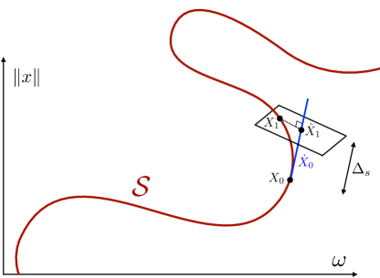
Figure 3: Pseudo-arclength continuation. By following the tangent vector to the solution branch and projecting into a suitable perpendicular plane, pseudo-arclength continuation is indifferent to fold bifurcations and allows for the following of more complicated solution curves.

3.2 From the polygon to the figure eight

Having introduced the pseudo-arclength continuation, we describe a numerical procedure to bifurcate away from the polygon equilibrium onto an off ($x,y$)-plane spatial family of choreographies, to detect a secondary bifurcation, to perform a branch switching, and finally to reach the figure eight choreography. This process requires a starting point $X_{0}$ (the polygon equilibrium) and a tangent vector $\dot{X}_{0}$ at the polygon.

3.2.1 Initiating the continuation at the polygon

Recall the definition of $x_{0}$ the polygon equilibrium (11) and $x_{1}$ the vector given by (12). Abusing slightly the notation, denote $x_{0},x_{1}\in\mathbb{C}^{N}$ the corresponding vectors of Fourier coefficients. More explicitly, $x_{0}=\left(0,0,u_{0},0,w_{0}\right)\in\mathbb{C}^{N}$ is defined by $u_{0}=\left((\delta_{\ell,0})_{|\ell|<m},0,0\right)\in\mathbb{C}^{3(2m-1)}$ and for $j=1,\dots,n-1$, $(w_{0})_{j}=\left(\frac{\delta_{\ell,0}}{2\sin j\pi/n}\right)_{|\ell|<m}\in\mathbb{C}^{2m-1}$. Here, $\delta_{\ell,k}$ denotes the Kronecker delta symbol. Moreover, $x_{1}=(0,0,u_{1},v_{1},0)$ is defined by $u_{1}=(0,0,u^{(3)}_{1})\in\mathbb{C}^{3(2m-1)}$ and $v_{1}=(0,0,v_{1}^{(3)})\in\mathbb{C}^{3(2m-1)}$ with $u^{(3)}_{1},v^{(3)}_{1}\in\mathbb{C}^{2m-1}$ given component-wise by

$$\left(u^{(3)}_{1}\right)_{\ell}=\begin{cases}i/2,&\ell=-1\\ -i/2,&\ell=1\\ 0,&\text{otherwise}\end{cases}\qquad\text{and}\qquad\left(v^{(3)}_{1}\right)_{\ell}=\begin{cases}1/2,&\ell=-1\\ 1/2,&\ell=1\\ 0,&\text{otherwise}.\end{cases}$$

Denote $\omega_{0}\,\stackrel{{\scriptstyle\mbox{\tiny{\raisebox{0.0pt}[0.0pt][0.0pt]{def}}}}}{{=}}\,\sqrt{s_{k}}$, $X_{0}\,\stackrel{{\scriptstyle\mbox{\tiny{\raisebox{0.0pt}[0.0pt][0.0pt]{def}}}}}{{=}}\,(x_{0},\omega_{0})$, and recall Proposition 1. Then $F(X_{0})=0\in\mathbb{C}^{N}$ and $D_{x}F(X_{0})x_{1}=0\in\mathbb{C}^{N}$. Denote $\dot{X}_{0}\,\stackrel{{\scriptstyle\mbox{\tiny{\raisebox{0.0pt}[0.0pt][0.0pt]{def}}}}}{{=}}\,(x_{1},0)\in\mathbb{C}^{N+1}$ and consider the $N\times(N+1)$ dimensional matrix $D_{X}F(X_{0})=[D_{x}F(X_{0})~{}D_{\omega}F(X_{0})]$. Hence, at the polygon $X_{0}$,

$$F(X_{0})=0\quad\text{and}\quad D_{X}F(X_{0})\dot{X}_{0}=0,$$

which provide with the data required to initiate the numerical pseudo-arclength continuation on the problem $F:\mathbb{C}^{N+1}\to\mathbb{C}^{N}$ as presented in Section 3.1. We fix the pseudo-arclength parameter (the continuation step size) to be $\Delta_{s}=10^{-3}$ and initiate the continuation.

3.2.2 Switching branches at the secondary bifurcation

Along the continuation, we monitor two quantities, namely the sign of the determinant of the derivative of the pseudo-arclength map given in (15) and the condition number of the derivative. If there is a change of sign in the determinant and if the condition number is above a certain threshold (in our case $10^{3}$), we declare having detected a secondary bifurcation and begin a bisection algorithm to converge to a (bifurcation) point $X_{\rm bif}$ at which the determinant of the derivative of pseudo-arclength map is approximatively zero. In this case, we numerically verify that $\dim\ker(D_{X}F(X_{\rm bif}))=2$, and we call $X_{\rm bif}$ a simple branching point. At $X_{\rm bif}$, there are two solution branches intersecting. Denote by $X_{\rm bif}^{(1)},X_{\rm bif}^{(2)}\in\mathbb{C}^{N+1}$ the two tangent vectors. See Figure 4 for a graphical representation of the situation.

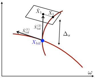
Figure 4: Intersection of two solution branches at a simple branching point. Analyzing the kernel at the bifurcation facilitates the branch switching.

Note that the exact tangent vectors $X_{\rm bif}^{(1)}$ and $X_{\rm bif}^{(2)}$ are not readily available and computing them accurately would require solving an algebraic bifurcation equation (e.g. see MR1159608 ), which we do not perform here. Instead consider $\phi_{1},\phi_{2}\in\mathbb{C}^{N+1}$ by any two vectors computed numerically (we use the singular value decomposition of $D_{X}F(X_{\rm bif})$ to do that) such that $\ker(D_{X}F(X_{\rm bif}))=\langle\phi_{1},\phi_{2}\rangle$. Since we expect this secondary bifurcation to be a generic pitchfork bifurcation with respect to the parameter $\omega$, we numerically set

$$\hat{X}_{\rm bif}^{(2)}\,\stackrel{{\scriptstyle\mbox{\tiny{\raisebox{0.0pt}[0.0pt][0.0pt]{def}}}}}{{=}}\,(\phi_{2})_{N+1}\phi_{1}-(\phi_{1})_{N+1}\phi_{2}\in\ker(D_{X}F(X_{\rm bif}))\approx X_{\rm bif}^{(2)}$$

so that it has a zero tangent contribution in the parameter $\omega$. We then set $X_{0}=X_{\rm bif}$ and $\dot{X}_{0}=\hat{X}_{\rm bif}^{(2)}$, and initiate the numerical pseudo-arclength continuation on the problem $F:\mathbb{C}^{N+1}\to\mathbb{C}^{N}$ as presented in Section 3.1.

Since the figure eight is expected to occur (according to Remark 2) at

$$\omega=2\sqrt{s_{1}}=\frac{1}{2}\sum_{j=1}^{n-1}\frac{1}{\sin(\pi j/n)},$$

we monitor the sign of the function $\omega\mapsto 2\sqrt{s_{1}}-\omega$ along the continuation on the second branch. When it changes sign, we fix $\omega=2\sqrt{s_{1}}$ and run Newton’s method to obtain the figure eight.

3.3 Stability

An important question is to consider the stability of choreographic solutions, and for this we put aside the symmetrized DDE formulation, and return to the original rotating $n$-body problem. That is, we start with the second order problem defined in Equation (2). Let $f\colon\mathbb{R}^{6n}\to\mathbb{R}^{6n}$ denote the corresponding first order vector field obtained by appending the velocity variables to the equation, and suppose that $\gamma\colon[0,T]\to\mathbb{R}^{6n}$ is a periodic solution of the problem. That is, assume that $T>0$ and that $\gamma(t)$ solves the ordinary differential equation $\gamma^{\prime}(t)=f(\gamma(t))$ for $t\in(0,T)$ with $\gamma(0)=\gamma(T)$.

The equation of first variation is the non-autonomous linear matrix initial value problem defined by

$$M^{\prime}(t)=Df(\gamma(t))M(t),\quad\quad\quad M(0)=\mbox{Id}.$$

The stability of the periodic orbit is determined by the eigenvalues of the monodromy matrix $M(T)$. We refer to the number of unstable eigenvalues of $M(T)$ as the Morse index of $\gamma$.

To compute the Monodromy matrix we numerically integrate the system of equations

$$\gamma^{\prime} =f(\gamma)$$

$$M^{\prime} =Df(\gamma)M$$

over the time interval $[0,T]$, where $T>0$ is the period of the orbit. We use a standard Runge-Kutta scheme built into MatLab (the standard rk45). The initial conditions are $\gamma(0)=\gamma_{0}$ and $M(0)=\mbox{Id}$, where $\gamma_{0}$ is a point on the periodic orbit. The initial conditions $\gamma_{0}$ are obtained exploiting the fact that we have already computed the Fourier coefficients of the trajectory of the $n$-th body using the DDE formulation. The Fourier series of the trajectories for the other $n-1$ bodies are recovered from the symmetries, and by evaluating the Fourier series we obtain an appropriate initial condition $\gamma_{0}\in\mathbb{R}^{6n}$ on the periodic orbit.

3.4 Numerical results

We applied successfully the numerical approach of Section 3.2 to the cases $N=3,5,7,9,11,13$ and $15$ bodies. Stability is computed as discussed in Section 3.3. Figure 5, illustrates the numerical continuation from the equilateral triangle to the figure eight for $N=3$ bodies, and illustrates also the analogous computation for $N=5$ bodies. The Morse indices are also reported along the branches. Similarly, see Figure 6 for the continuations for $N=7$ and $N=9$ bodies. In the case of $N=11$, $N=13$ and $N=15$ bodies, we do not report the Morse indices, as the stability of the orbits change too frequently along the continuation branch. But the bifurcation diagrams are given in Figure 7.

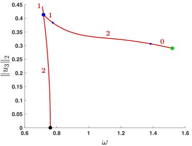
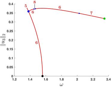
Figure 5: Continuation from the triangle (the black dot) to the figure eight (the green dot) for $N=3$ (left) and $N=5$ (right) bodies. The different Morse indices are portrayed along the branches.

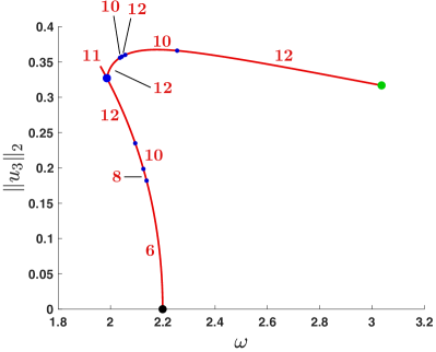
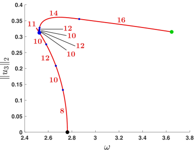
Figure 6: Continuation from the triangle (the black dot) to the figure eight (the green dot) for $N=7$ (left) and $N=9$ (right) bodies. The different Morse indices are portrayed along the branches.

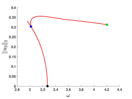
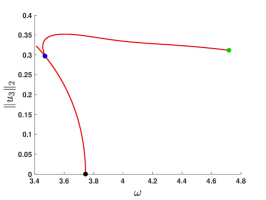
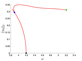
Figure 7: Continuation from the triangle (the black dot) to the figure eight (the green dot) for $N=11$ (left), $N=13$ (center) and $N=15$ (right) bodies.

We remark that bifurcation diagrams in the cases $N=3,5,7,9$ exhibit some qualitative differences. Most notably the angle between the Lyapunov family and the axial family changes dramatically in these cases. The diagrams in the cases of $N=9,11,13,15$ on the other hand are very similar, and exhibit a kind of convergence to a universal profile. Again, the existence of such a profile is pure conjecture at this point. But the numerics seem to bear it out.

It was observed early on that the three body figure eight choreography is linearly stable (Morse index zero). Indeed, the KAM stability of the three body eight was established by Kapela and Simó KaSi07 ; KaSi17 using computer-assisted methods. For five or more bodies no stable eights have ever been reported, and indeed we observe quite large Morse indices along the axial continuation branch in all but the three body case.

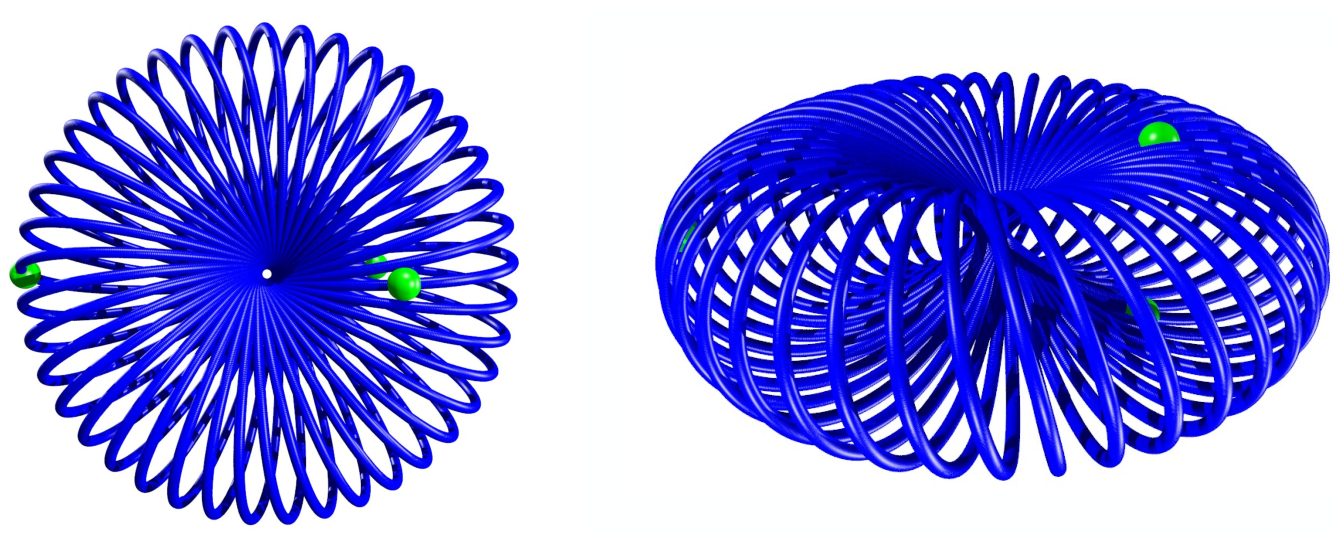
Figure 8: A stable spatial three body choreography: a spatial choreography in the three body axial family near the three body eight. The orbit is linearly stable in the sense of Hamiltonian systems: that is, all of it’s Floquet multipliers are on the unit circle. This choreography is a $(p,q)$-torus knot with $p=19$ and $q=41$. See renatoAnimations for an interactive animation.

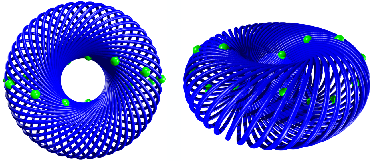
Figure 9: A spatial fifteen body choreography: a spatial choreography in the fifteen body axial family along the branch that contains the fifteen body eight. The orbit is a $(p,q)$-torus knot choreography with $p=31$ and $q=47$.

Remark 3 (A stable spatial three body choreography)

A periodic orbit is linearly stable in the sense of Hamiltonian systems if all of its Floquet multipliers are on the unit circle in $\mathbb{C}$. It was observed early on, based on numerical evidence, that the three body figure eight seemed to be linearly stable in the sense of Hamiltonian systems. This observation was eventually proven by Kapela and Simó KaSi07 using computer assisted methods of proof. Indeed, the same authors prove KAM stability in KaSi17 , again using computer-assisted methods.

It is an open question as to wether or not there exist other stable eights for higher numbers of bodies, and our numerical experiments seem to suggest that the answer to this question is “no”. On the other hand, linear stability is a robust property, so that nearby periodic orbits in the continuation class of the three body eight are also stable. By numerically exploring the continuation class we have been able to find many spatial choreographies which are linearly stable. One such orbit is illustrated in Figure 9.

4 Conclusion

Building on previous numerical studies of $n$-body eights Mo93 ; Si00 ; MR1919833 and in particular numerical continuation results for choreographies found in MR2429679 ; CaDoGa18 , we applied classical numerical continuation methods to the periodic solutions of a delay differential equation (DDE) describing choreographic motion in the gravitational $n$-body problem. The DDE formulation is given ourTorusKnots , and has two distinct advantages over working directly with the standard $n$-body equations of motion derived from Newton’s Laws. In the first place, periodic solutions of the DDE satisfying a certain number theoretic condition correspond to choreographies rather than to arbitrary $n$-body periodic motions. Second, the DDE reduces to a system of six scalar equations (with delays), regardless of the number of bodies under consideration: adding more bodies introduces new terms to the nonlinearity rather than increasing the dimension of the system.

The $n$-gon appears as a constant/equilibrium solution of the DDE, and a linear stability analysis shows that there is a single vertical Lyapunov family of periodic orbits in the center manifold. Using the explicit first order formulas for the vertical family derived in GaIz11 ; MR3554377 we are able to start the numerical continuation of the vertical family in an automatic way for any desired number of bodies. For every odd $n$ between $3$ and $15$ we continue the vertical family with respect to energy/frequency, checking for the eight as we move along the branch. Note that we recover the earlier three and seven body results from MR2429679 ; CaDoGa18 , and also obtain new examples connecting the $n$-gon to the eight.

In each case we find that the $n$-body eight appears shortly after a symmetry breaking bifurcation from the $n$-gon’s branch. Moreover, after leaving the $n$-gon using the formulas developed in GaIz11 ; MR3554377 , there appears to be one and only one bifurcation between the $n$-gon and the eight. We stress that this is another advantage of performing the continuation in the DDE rather than using the $n$-body equations of motion: continuation of choreographies in the full $n$-body problem can result in additional bifurcations, as non-choreography periodic solutions may bifurcate from choreographies. The fact that, in the symmetrized setting, a single dynamical mechanism appears to organize the transition from $n$-gon to eight leads us to generalize Marchal’s conjecture (described in fijozHabilatation and again in the introduction of the present work) to any odd number of bodies.

We remark that – even in the case of three bodies – there appears as of yet to be no mathematically rigorous proof of Marchal’s conjecture, much less any of it’s generalizations to more bodies. A very interesting avenue of future research would be to develop such proofs. Mathematically rigorous results about $n$-body choreographies come in two main varieties: variational methods and computer-assisted proofs. We refer the interested reader to the works of ChMo00 ; BaTe04 ; TeVe07 ; FeTe04 ; BT04 for a much more complete discussion of the literature on variational methods for choreography problems. Computer-assisted methods of proof for $n$-body choreographies which apply constructive geometric arguments in the full $n$-body state space are found in the works of KaZg03 ; MR2185163 ; KaSi07 ; KaSi17 . A very interesting work which uses both variational and computer-assisted approaches is MR2259202 . The author’s aforementioned work in ourTorusKnots uses a-posteriori analysis for Fourier spectral methods to prove the existence of spatial torus knot choreographies using the delay differential equation set up exploited in the present work.

As is well known and already mentioned in the introduction, there are technical difficulties applying variational methods to continuation branches which encounter bifurcations. On the other hand, mathematically rigorous computer-assisted methods for studying continuous branches of periodic orbits are by now quite advanced. This is true even in the case of DDEs, and we refer for example to the work of MR2487806 ; MR2711226 ; jonopJP_Kon ; MR2630003 ; Le18 ; JB_Elena_Cont_PO . Moreover, methods of computer-assisted proof have been developed for proving the existence of, and continuing through, a number of infinite dimensional bifurcations. See for example the work of MR3779642 ; jono_jones ; MR2679365 ; MR3792794 ; MR3808252 .

While existing methods from the works just cited do not cover the symmetry breaking bifurcations needed to prove instances of the generalized Marchal’s conjecture, we believe an appropriate framework for the envisioned proofs can be obtained by extending/adapting these works. Moreover, the out of plane bifurcation from the Lagrangian $n$-gon can be handled using the results of GaIz11 ; GaIz13 , as in the present work. Computer-assisted proofs of several cases of the generalized Marchal’s conjecture, the ones for which we have presented numerical evidence in the present manuscript, are the subject of a work in preparation by the authors.

References

- (1) H. Poincaré. Les méthodes nouvelles de la mécanique céleste. Tome I. Les Grands Classiques Gauthier-Villars. [Gauthier-Villars Great Classics]. Librairie Scientifique et Technique Albert Blanchard, Paris, 1987. Solutions périodiques. Non-existence des intégrales uniformes. Solutions asymptotiques. [Periodic solutions. Nonexistence of uniform integrals. Asymptotic solutions], Reprint of the 1892 original, With a foreword by J. Kovalevsky, Bibliothèque Scientifique Albert Blanchard. [Albert Blanchard Scientific Library].
- (2) H. Poincaré. Les méthodes nouvelles de la mécanique céleste. Tome II. Les Grands Classiques Gauthier-Villars. [Gauthier-Villars Great Classics]. Librairie Scientifique et Technique Albert Blanchard, Paris, 1987. Méthodes de MM. Newcomb, Gyldén, Lindstedt et Bohlin. [The methods of Newcomb, Gyldén, Lindstedt and Bohlin], Reprint of the 1893 original, Bibliothèque Scientifique Albert Blanchard. [Albert Blanchard Scientific Library].
- (3) H. Poincaré. Les méthodes nouvelles de la mécanique céleste. Tome III. Les Grands Classiques Gauthier-Villars. [Gauthier-Villars Great Classics]. Librairie Scientifique et Technique Albert Blanchard, Paris, 1987. Invariant intégraux. Solutions périodiques du deuxième genre. Solutions doublement asymptotiques. [Integral invariants. Periodic solutions of the second kind. Doubly asymptotic solutions], Reprint of the 1899 original, Bibliothèque Scientifique Albert Blanchard. [Albert Blanchard Scientific Library].
- (4) G. H. Darwin. Periodic Orbits. Acta Math., 21(1):99–242, 1897.
- (5) Forest Ray Moulton. Differential equations. Dover Publications, Inc., New York, N.Y., 1958.
- (6) E. Strömgren. Connaissance actuelle des orbites dans le probleme des trois corps. Bull. Astronom., 9(2):87–130, 1933.
- (7) Alain Chenciner. Poincaré and the three-body problem. In Henri Poincaré, 1912–2012, volume 67 of Prog. Math. Phys., pages 51–149. Birkhäuser/Springer, Basel, 2015.
- (8) Jürgen Moser. Stable and random motions in dynamical systems. Princeton Landmarks in Mathematics. Princeton University Press, Princeton, NJ, 2001. With special emphasis on celestial mechanics, Reprint of the 1973 original, With a foreword by Philip J. Holmes.
- (9) Kenneth R. Meyer, Glen R. Hall, and Dan Offin. Introduction to Hamiltonian dynamical systems and the -body problem, volume 90 of Applied Mathematical Sciences. Springer, New York, second edition, 2009.
- (10) Victor Szebehely. Theory of Orbits: the restricted problem of three bodies. Academic Press Inc., 1967.
- (11) J.L. Lagrnge. Essai sur le probléme des trois corps. Euvres, 6:229–331, 1772.
- (12) R. Hoppe. Erweiterung der bekannten speciallösung des dreikörperproblems. Archives of Mathematical Physics, 64(218), 1879.
- (13) L. M. Perko and E. L. Walter. Regular polygon solutions of the -body problem. Proc. Amer. Math. Soc., 94(2):301–309, 1985.
- (14) C Moore. Braids in classical gravity. Physical Review Letters, 70:3675–3679, 1993.
- (15) Alain Chenciner and Richard Montgomery. A remarkable periodic solution of the three-body problem in the case of equal masses. Ann. of Math. (2), 152(3):881–901, 2000.
- (16) Carles Simó. Dynamical properties of the figure eight solution of the three-body problem. In Celestial mechanics (Evanston, IL, 1999), volume 292 of Contemp. Math., pages 209–228. Amer. Math. Soc., Providence, RI, 2002.
-
(17)
Renato C. Calleja.
Anamations of some choreographies.
https://mym.iimas.unam.mx/renato/choreographies/Marchal.html, 2020. - (18) Jacques Féjoz. Periodic and quasi-periodic motions in the many-body problem dynamical systems [math.ds]. Mémoire D’Habilitation, Université Perre et Marie Curie - Paris VI, 2010.
- (19) Alain Chenciner. Four lectures on the -body problem. In Hamiltonian dynamical systems and applications, NATO Sci. Peace Secur. Ser. B Phys. Biophys., pages 21–52. Springer, Dordrecht, 2008.
- (20) Claudia Wulff and Andreas Schebesch. Numerical continuation of Hamiltonian relative periodic orbits. J. Nonlinear Sci., 18(4):343–390, 2008.
- (21) Alain Chenciner and Jacques Féjoz. The flow of the equal-mass spatial 3-body problem in the neighborhood of the equilateral relative equilibrium. Discrete Contin. Dyn. Syst. Ser. B, 10(2-3):421–438, 2008.
- (22) A. Chenciner and J. Féjoz. Unchained polygons and the -body problem. Regul. Chaotic Dyn., 14(1):64–115, 2009.
- (23) C. García-Azpeitia and J. Ize. Global bifurcation of polygonal relative equilibria for masses, vortices and dNLS oscillators. J. Differential Equations, 251(11):3202–3227, 2011.
- (24) C. García-Azpeitia and J. Ize. Global bifurcation of planar and spatial periodic solutions from the polygonal relative equilibria for the -body problem. J. Differential Equations, 254(5):2033–2075, 2013.
- (25) Carles Simó. New families of solutions in -body problems. In European Congress of Mathematics, Vol. I (Barcelona, 2000), volume 201 of Progr. Math., pages 101–115. Birkhäuser, Basel, 2001.
- (26) Davide L. Ferrario and Susanna Terracini. On the existence of collisionless equivariant minimizers for the classical -body problem. Invent. Math., 155(2):305–362, 2004.
- (27) Renato Calleja, Eusebius Doedel, and Carlos García-Azpeitia. Symmetries and choreographies in families that bifurcate from the polygonal relative equilibrium of the -body problem. Celestial Mech. Dynam. Astronom., 130(7):Art. 48, 28, 2018.
- (28) Renato Calleja, Carlos García-Azpeitia, J.P. Lessard, and J. D. Mireles James. Torus knot choreographies in the n-body problem. (Accepted for publication in Nonlinearity), 2020.
- (29) H. B. Keller. Lectures on numerical methods in bifurcation problems, volume 79 of Tata Institute of Fundamental Research Lectures on Mathematics and Physics. Published for the Tata Institute of Fundamental Research, Bombay, 1987. With notes by A. K. Nandakumaran and Mythily Ramaswamy.
- (30) Eusebius Doedel, Herbert B. Keller, and Jean-Pierre Kernévez. Numerical analysis and control of bifurcation problems. I. Bifurcation in finite dimensions. Internat. J. Bifur. Chaos Appl. Sci. Engrg., 1(3):493–520, 1991.
- (31) Tomasz Kapela and Carles Simó. Computer assisted proofs for nonsymmetric planar choreographies and for stability of the Eight. Nonlinearity, 20(5):1241–1255, 2007. With multimedia enhancements available from the abstract page in the online journal.
- (32) Tomasz Kapela and Carles Simó. Rigorous KAM results around arbitrary periodic orbits for Hamiltonian systems. Nonlinearity, 30(3):965–986, 2017.
- (33) Alain Chenciner, Joseph Gerver, Richard Montgomery, and Carles Simó. Simple choreographic motions of bodies: a preliminary study. In Geometry, mechanics, and dynamics, pages 287–308. Springer, New York, 2002.
- (34) Jaime Burgos-García. Families of periodic orbits in the planar Hill’s four-body problem. Astrophys. Space Sci., 361(11):Paper No. 353, 21, 2016.
- (35) Vivina Barutello, Davide L. Ferrario, and Susanna Terracini. Symmetry groups of the planar three-body problem and action-minimizing trajectories. Arch. Ration. Mech. Anal., 190(2):189–226, 2008.
- (36) Susanna Terracini and Andrea Venturelli. Symmetric trajectories for the -body problem with equal masses. Arch. Ration. Mech. Anal., 184(3):465–493, 2007.
- (37) V. Barutello and S. Terracini. Action minimizing orbits in the -body problem with simple choreography constraint. Nonlinearity, 17(6):2015–2039, 2004.
- (38) Tomasz Kapela and Piotr Zgliczyński. The existence of simple choreographies for the -body problem—a computer-assisted proof. Nonlinearity, 16(6):1899–1918, 2003.
- (39) Tomasz Kapela. -body choreographies with a reflectional symmetry—computer assisted existence proofs. In EQUADIFF 2003, pages 999–1004. World Sci. Publ., Hackensack, NJ, 2005.
- (40) Gianni Arioli, Vivina Barutello, and Susanna Terracini. A new branch of Mountain Pass solutions for the choreographical 3-body problem. Comm. Math. Phys., 268(2):439–463, 2006.
- (41) Marcio Gameiro, Jean-Philippe Lessard, and Konstantin Mischaikow. Validated continuation over large parameter ranges for equilibria of PDEs. Math. Comput. Simulation, 79(4):1368–1382, 2008.
- (42) Jean-Philippe Lessard. Validated continuation for infinite dimensional problems. ProQuest LLC, Ann Arbor, MI, 2007. Thesis (Ph.D.)–Georgia Institute of Technology.
- (43) Jonathan Jaquette, Jean-Philippe Lessard, and Konstantin Mischaikow. Stability and uniquness of slowly oscillating periodic solutions to wright’s equation. Journal of Differential Equations, 11:7263–7286, 2017.
- (44) Jan Bouwe van den Berg, Jean-Philippe Lessard, and Konstantin Mischaikow. Global smooth solution curves using rigorous branch following. Math. Comp., 79(271):1565–1584, 2010.
- (45) Jean-Philippe Lessard. Continuation of solutions and studying delay differential equations via rigorous numerics. In Rigorous numerics in dynamics, volume 74 of Proc. Sympos. Appl. Math., pages 81–122. Amer. Math. Soc., Providence, RI, 2018.
- (46) Jan Bouwe van den Berg and Elena Queirolo. A general framework for validated continuation of periodic orbits in systems of polynomial ODEs. J. Computational Dynamics, 8:59–97, 2021.
- (47) Jan Bouwe van den Berg and Jonathan Jaquette. A proof of Wright’s conjecture. J. Differential Equations, 264(12):7412–7462, 2018.
- (48) Jonathan Jaquette. A proof of Jones’ conjecture. J. Differential Equations, 2019.
- (49) Gianni Arioli and Hans Koch. Computer-assisted methods for the study of stationary solutions in dissipative systems, applied to the Kuramoto-Sivashinski equation. Arch. Ration. Mech. Anal., 197(3):1033–1051, 2010.
- (50) Thomas Wanner. Computer-assisted bifurcation diagram validation and applications in materials science. In Rigorous numerics in dynamics, volume 74 of Proc. Sympos. Appl. Math., pages 123–174. Amer. Math. Soc., Providence, RI, 2018.
- (51) Jean-Philippe Lessard, Evelyn Sander, and Thomas Wanner. Rigorous continuation of bifurcation points in the diblock copolymer equation. J. Comput. Dyn., 4(1-2):71–118, 2017.