^aInstituto de Física Teórica (IFT) UAM-CSIC, Campus de Cantoblanco, 28049, Madrid, Spain
^bDepartamento de Física Teórica, Universidad Autónoma de Madrid (UAM), Campus de Cantoblanco, 28049 Madrid, Spain
^cSchool of Physics, Korea Institute for Advanced Study, Seoul 02455, Korea
^d Université Paris-Saclay, CNRS/IN2P3, IJCLab, 91405 Orsay, France
^eWilliam I. Fine Theoretical Physics Institute, School of Physics and Astronomy, University of Minnesota, Minneapolis, MN 55455, USA
^fSchool of Physics and Astronomy, University of Minnesota, Minneapolis, MN 55455, USA

ABSTRACT

We analyze in detail the perturbative decay of the inflaton oscillating about a generic form of its potential $V(\phi)=\phi^{k}$, taking into account the effects of non-instantaneous reheating. We show that evolution of the temperature as a function of the cosmological scale factor depends on the spin statistics of the final state decay products when $k>2$. We also include the inflaton-induced mass of the final states leading to either kinematic suppression or enhancement if the final states are fermionic or bosonic respectively. We compute the maximum temperature reached after inflation, the subsequent evolution of the temperature and the final reheat temperature. We apply our results to the computation of the dark matter abundance through thermal scattering during reheating. We also provide an example based on supersymmetry for the coupling of the inflaton to matter.

December 2020

1 Introduction

The inflationary paradigm [1] is well ensconced in the standard model of modern cosmology. Specific models of inflation can be tested by observations, most notably by the anisotropy spectrum of the cosmic microwave background (CMB) [2]. A necessary feature of all inflationary models is the ability to amply reheat the universe following the period of exponential expansion, leading to a radiation dominated epoch. Often, perturbative reheating occurs as the inflaton begins a series of oscillations about a minimum. When massive inflaton oscillations dominate the energy density, the universe expands as if it were matter dominated until the inflaton decays to relativistic particles which thermalize and reheat the Universe [3, 4].

A commonly used approximation to reheating is a pair of assumptions: instantaneous decay and instantaneous thermalization. There has been a substantial amount of work which takes into account non-instantaneous reheating [5, 7, 6, 8, 9, 10, 11] or thermalization [12, 13, 14, 15] after inflation. In this work, we maintain the instantaneous thermalization approximation, but consider in detail the evolution of the reheat process for general decays of the inflaton. It is common to assume that after inflation, a massive inflaton begins oscillating about a minimum. As decays begin, the decay products thermalize quickly and produce a thermal bath with a maximum temperature $T_{\rm max}$. Subsequently, as inflaton decays continue, the temperature falls with the cosmological scale factor, but not as $T\sim a^{-1}$ as is common for an adiabatically expanding universe. Instead, the temperature decreases more slowly, $T\sim a^{-3/8}$, as new particles are introduced into the thermal bath from continuing decays. The reheat temperature is often defined when the energy density in the newly created radiation bath is equal to the energy density of the inflaton oscillations.

In [16, 9], it was noted that the evolution of the thermal bath depends on the form of the potential leading to inflaton oscillations. For example, in a class of inflation models based on attractor solutions known as ‘T’ models [17], the potential in the vicinity of the minimum takes the form $V\sim\phi^{k}$, rather than simply $V\sim m^{2}\phi^{2}$. In this case, it was found [9] that since the effective mass of the inflaton is now field dependent, its decay rate is as well, thus affecting the evolution of the temperature so that $T\sim a^{-(3k-3)/(2k+4)}$. The maximum temperature as well as the reheat temperature are also affected. Here, we will show that the evolution of the temperature depends not only on $k$, but also on the spin statistics of the final state particles produced during reheating.

The evolution of the temperature may directly affect the production of dark matter after inflation. While weakly interacting dark matter candidates will come into full equilibrium for sufficiently high reheat temperatures, superweakly interacting candidates such as the gravitino [18, 19, 20, 21, 4] may be produced but never achieve thermal equilibrium before the expansion of the Universe (given by the Hubble parameter, $H$) dominates over their production rate. The same mechanism, now generally referred to as freeze-in, applies to a wider class of dark matter candidates known as feebly interacting massive particles or FIMPs [22, 10, 23, 24, 16]. Depending on the temperature dependence of its production rate, the relic density of a FIMP may depend on the either the maximum temperature achieved after inflation, $T_{\rm max}$, the reheat temperature, $T_{\rm RH}$, or both. For example, the gravitino in weak scale supersymmetric models is primarily dependent on the reheat temperature [4, 19, 20, 21, 25, 26, 27, 28, 29, 30, 31, 32, 33, 34, 35, 36, 37, 39, 38, 40, 7, 41], whereas the gravitino in high-scale supersymmetric models [42, 6, 43], depends on both $T_{\rm max}$ and $T_{\rm RH}$. Other examples include dark matter particles produced by the exchange of a massive $Z^{\prime}$ [44] (that can be present in SO(10) constructions [45]) or models with a moduli portal [46] in emergent/modified gravity [47]. Even massive spin-2 [48] or Kaluza Klein [49] fields can play the role of an effective portal to avoid overabundance.

In all of these constructions, which can be called UV freeze-in [8, 16], the importance of the evolution of the temperature during reheating is extremely important. It was shown in [7] that a large enhancement in the relic density is expected for models whose dark matter production cross-sections are of the form $\langle\sigma v\rangle\propto\frac{T^{n}}{\Lambda^{n+2}}$, with $n\geq 6$. While $n=0$ for the production cross section for weak scale gravitinos, $n=6$ in high-scale supersymmetric models, and $n=4$ in other spin-$\frac{3}{2}$ dark matter models [50]. The evolution of the temperature during reheating also plays a role for dark matter produced directly from inflaton decays, either at the tree level [40, 7, 6, 9], or at the loop level [51].

Noting the importance of inflaton decay on the abundance of dark matter in these models, it should not be a surprise that the shape of potential during inflaton oscillations also plays a role [16, 9]. A potential of the form $V\sim\phi^{k}$, affects not only the equation of state and the hence the expansion rate of the universe, but also the decay rate of the inflaton which becomes field dependent for $k>2$. In this paper, we extend the recent work of [9] and show further that in models with $k\neq 2$, the evolution of the reheating process also depends on the statistics of the final state particles predominantly produced during inflaton decay. Furthermore, the masses of the final state particles may also be field dependent leading to kinematic suppressions or enhancements. Below we derive the temperature dependence of the scale factor, the maximum temperature, and the reheat temperature, for generic models with $k\geq 2$, and inflaton decays into fermion/anti-fermion pairs, and boson pairs, as well as inflaton annihilations into boson pairs. We also derive the thermally produced dark matter abundance and provide an example based on weak scale supersymmetry.

The paper is organized as follows: In section 2, we consider the effect of a potential of the form $V\sim\phi^{k}$ on the equation of state and the equations of motion governing inflaton oscillations. In section 3, we consider the decay of the inflaton to fermion and boson pairs as well as annihilations to boson pairs. The kinematic details of these rates are derived in the Appendix. The coupling of the inflaton leads to field dependent final state masses which in turn leads to a suppression in the decays to fermions, and an enhancement in the decays to bosons. In section 4, we work out the general solutions for the temperature evolution during the reheat process and derive $T_{\rm max}$ and $T_{\rm RH}$. These results are used to compute the thermal production of dark matter in section 5. A concrete example based on weak scale supersymmetry is given in section 6. Finally in section 7, we discuss the limitations of our work and summarize our results.

2 Post-Inflationary Inflaton Oscillations

In most models of inflation, the period of exponential expansion is followed by a period of inflaton oscillations about a minimum. These oscillations continue until the inflaton decays, and the reheating process begins [3]. The perturbative reheating approximation, fundamental for the description of post-inflationary dynamics in the small coupling limit, more often than not relies on the assumption that the inflaton is a massive field governed by the dynamics of a quadratic potential, that is $V(\phi)\simeq\frac{1}{2}m_{\phi}^{2}\phi^{2}$ about the minimum which we assume is situated at the origin. If one, for simplicity, assumes that the decay of the inflaton proceeds through fermion production, $\phi\rightarrow\bar{f}f$, then its decay rate can simply be parametrized as

$$\Gamma_{\phi}\;\equiv\;\frac{y^{2}}{8\pi}m_{\phi}\,,$$ (2.1)

where $y$ denotes the effective Yukawa coupling that determines the strength of the decay. This decay rate is a constant number, up to the running of $y$, and leads to the exponential decay of the inflaton field. Under the assumption that the decay products of $\phi$ are relativistic at their creation, and thermalize on a time scale much shorter than $\Gamma_{\phi}^{-1}$, they form a thermal bath that eventually leads to a universe dominated by radiation following the complete depletion of the energy density of $\phi$. The maximum temperature of this plasma after the decay of the inflaton is referred to as the reheating temperature, and is generically parametrized as

$$T_{\rm RH}\;=\;\left(\frac{40}{g_{\rm RH}\pi^{2}}\right)^{1/4}\left(\frac{\Gamma_{\phi}M_{P}}{c}\right)^{1/2}\,.$$ (2.2)

Here, $g_{\rm RH}$ denotes the effective number of relativistic degrees of freedom at reheating time, and $c$ is an $\mathcal{O}(1)$ constant whose value depends on the convention chosen to define the reheating time. For example, $c\simeq 1$ if one assumes $t_{\rm RH}=\frac{3}{2}H(T_{\rm RH})=\Gamma_{\phi}^{-1}$, and $c\simeq 5/3$ if instead $\rho_{\phi}(t_{\rm RH})=\rho_{r}(t_{\rm RH})$, where $\rho_{\phi}$ and $\rho_{R}$ denote the energy densities of the inflaton and its decay products, respectively.

As a first approximation, a quadratic potential seems natural and is a feature of many cosmological inflationary models, among them the Starobinsky model [52, 53, 54]. However, other inflationary models do not share this feature. Most notably, some $\alpha$-attractor models have minima about which $V(\phi)\sim\phi^{k}$ for even $k$, e.g. the T-models [17]

$$V(\phi)\;=\;\lambda M^{4}\left[\sqrt{6}\tanh\left(\frac{\phi}{\sqrt{6}M}\right)\right]^{k}\,,$$ (2.3)

which can be easily derived in no-scale models of supergravity [9]. Here $M$ is a characteristic mass scale of the model in question, which without loss of generality we take to be $M=M_{P}$, where the reduced Planck is $M_{P}=1/\sqrt{8\pi\,G}\simeq 2.4\times 10^{18}\,{\rm GeV}$. A potential with $k>2$ will lead to anharmonic oscillations of the inflaton field during reheating. As we discuss in more detail below, this anharmonicity is reflected in the fact that the energy density of the inflaton no longer redshifts as matter. For example, for $k=4$, $\rho_{\phi}$ redshifts like radiation, modifying drastically the reheating process when compared to the vanilla $k=2$ scenario. Moreover, for $k=4$, the tree-level vacuum fluctuation of the inflaton would be massless, and its direct decay would be impossible. Nevertheless, the decay of the oscillating inflaton condensate is possible, and in the adiabatic limit it can be described by the decay of a scalar field with a time-dependent effective mass as was recently shown in [55, 9]. Another remarkable consequence of this fact is the different time-dependence of the effective decay rate depending on the quantum statistics of the inflaton decay products.

Furthermore, the production of dark matter during reheating will be affected by these considerations, especially in models where the production rate is highly dependent on the energy (in other words on the temperature $T$) of the scattering particles. In this work, we analyze in detail the consequences of non-quadratic inflaton-potential on the reheating processes as well as the perturbative dark matter production at the end of inflation.

We begin by considering the inflaton potential given in Eq. (2.3). About the origin, the potential can be expanded to give

$$V(\phi)\;=\;\lambda\frac{\phi^{k}}{M_{P}^{k-4}}\,,\qquad\phi\ll M_{P}\,.$$ (2.4)

Of course other inflationary potentials can be expanded about their minimum to give a similar form as that in Eq. (2.4). For example, in Starobinsky inflation, we have $k=2$ as the inflaton has a well defined mass. After the exponential expansion associated with inflation, and during reheating, the inflaton will undergo damped oscillations about $\phi=0$. Ignoring decay for now, the equation of motion for $\phi$ is

$$\ddot{\phi}+3H\dot{\phi}+V^{\prime}(\phi)\;=\;0\,,$$ (2.5)

which in terms of the energy density and pressure stored in the scalar field

$$\rho_{\phi}=\frac{1}{2}\dot{\phi}^{2}+V(\phi);~{}~{}~{}P_{\phi}=\frac{1}{2}\dot{\phi}^{2}-V(\phi)\,,$$ (2.6)

can be written as

$$\dot{\rho}_{\phi}+3H(\rho_{\phi}+P_{\phi})=0\,,$$ (2.7)

where $H=\frac{\dot{a}}{a}$ is the Hubble parameter, and $a$ is the cosmological scale factor.

The time dependence of the inflaton after inflation, is given by the solution of (2.5) and can be approximately parametrized as

$$\phi(t)=\phi_{0}(t)\cdot\mathcal{P}(t)\,,$$

where the function $\mathcal{P}(t)$ is quasi-periodic and encodes the (an)harmonicity of the short time-scale oscillations in the potential. The envelope $\phi_{0}(t)$ encodes the effect of redshift and decay, and varies on longer time-scales.

When we include the effects of inflaton decay, the equation of motion for $\phi$ can be written as

$$\ddot{\phi}+(3H+\Gamma_{\phi})\dot{\phi}+V^{\prime}(\phi)\;=\;0\,.$$ (2.8)

Provided that we assume that the decay of the inflaton is relatively slow, i.e. the oscillation time-scale is much shorter than the decay and redshift time-scales, multiplication of (2.5) by $\phi$ and averaging over one oscillation leads to

$$\langle\dot{\phi}^{2}\rangle\;\simeq\;\langle\phi V^{\prime}(\phi)\rangle\,.$$ (2.9)

For a potential of the form (2.4), this implies that

$$\rho_{\phi}\simeq\frac{1}{2}\langle\dot{\phi}^{2}\rangle+\langle V(\phi)\rangle\simeq\frac{k+2}{2}\langle V(\phi)\rangle=V(\phi_{0})\,,$$ (2.10)

$$P_{\phi}\simeq\frac{1}{2}\langle\dot{\phi}^{2}\rangle-\langle V(\phi)\rangle\simeq\frac{k-2}{2}\langle V(\phi)\rangle=\frac{k-2}{k+2}V(\phi_{0})\,,$$ (2.11)

where we used $\langle{\cal P}^{k}\rangle=\frac{2}{k+2}$ so that $\langle V(\phi)\rangle=\frac{2}{k+2}V(\phi_{0})$. The equation of motion (2.5) can then be recast as

$$\dot{\rho}_{\phi}+3H(1+w_{\phi})\rho_{\phi}\;\simeq\;-\Gamma_{\phi}(1+w_{\phi})\rho_{\phi}\,,$$ (2.12)

where the equation-of-state parameter $w_{\phi}=\frac{P_{\phi}}{\rho_{\phi}}$ is given by

$$w_{\phi}\;=\;\frac{k-2}{k+2}\,.$$ (2.13)

The analogous equation for the evolution of the radiation density produced by inflaton decay or scattering (which we assume is in thermal equilibrium) is

$$\dot{\rho}_{R}+4H\rho_{R}\;\simeq\;(1+w_{\phi})\Gamma_{\phi}(t)\rho_{\phi}\,,$$ (2.14)

which together with the Friedmann equation

$$\rho_{\phi}+\rho_{R}\;=\;3H^{2}M_{P}^{2}\,,$$ (2.15)

allows one to solve for $\rho_{\phi}(t),\rho_{R}(t)$, and $a(t)$ simultaneously and effectively for $\rho_{\phi}(a)$ and $\rho_{R}(a)$. Comparing (2.8) and (2.12) we note that the dissipation rate from particle production for the inflaton field and energy densities differ by the constant factor $1+w_{\phi}=\frac{2k}{k+2}$  [56, 57]. The rate of decay for $\phi$ (and thus the number density $n_{\phi}$) is different from the rate of decay for $\rho_{\phi}$, which depends on the nature of the inflaton field (dust, radiation, cosmological constant, quintessence…). For a microscopic account of this difference we refer the interested reader to Appendix A. To solve the equation for $\rho_{\phi}$, we must first determine the expression of the width $\Gamma_{\phi}$ as a function of $\phi$.

3 Inflaton Decay and Annihilation

Once the inflaton couples to Standard Model fields or dark matter, its oscillations are severely damped by decays. To stay as general as possible, we consider the following possible contributions to the Lagrangian leading to decay or annihilation:

$$\mathcal{L}\supset\begin{cases}y\phi\bar{f}f&\phi\to\bar{f}f\\ \mu\phi bb&\phi\to bb\\ \sigma\phi^{2}b^{2}&\phi\phi\to bb,\end{cases}$$ (3.1)

with $f\,(b$) standing for a fermionic (bosonic) final state. The Yukawa-like coupling, $y$ and the four-point coupling, $\sigma$, are dimensionless, and $\mu$ is a dimensionful coupling. We note that, although our analysis will be limited to these three scenarios, our formalism can extended for more exotic inflaton-matter couplings in a relatively straightforward way.

Let us consider first the decay channel into two fermions. The rate is given by

$$\Gamma_{\phi\rightarrow\bar{f}f}(t)\equiv\ \frac{y_{{\rm{\it eff}}}^{2}(k)}{8\pi}m_{\phi}(t)~{},$$ (3.2)

where we have introduced the effective Yukawa coupling $y_{{\rm{\it eff}}}(k)\neq y$ obtained after averaging over one oscillation, and $m_{\phi}$ is defined by

$$m_{\phi}^{2}(t)\;\equiv\;V^{\prime\prime}(\phi_{0}(t))\;=\;k(k-1)\lambda M_{P}^{2}\left(\frac{\phi_{0}(t)}{M_{P}}\right)^{k-2}\,.$$ (3.3)

The function $y_{{\rm{\it eff}}}(k)$ includes sub-leading corrections, and must be evaluated numerically [58, 59]. It is different from $y$ because for $k\neq 2$, the inflaton mass depends on the oscillations of the field $\phi(t)$ and renders the lifetime computation slightly more complicated, and must include the mean of several oscillations. In (3.2) the time dependence of $m_{\phi}(t)$ is included in the envelope $\phi_{0}(t)$ only, which will be our main dynamical parameter during all our analysis. Note that this is analogous to $\rho_{\phi}=V(\phi_{0})$ (2.10) which is defined as function of the envelope. This can be understood by noticing that at the top of an oscillation, $\dot{\phi}$ is zero, and the inflaton behaves like a massive particle at rest. However, for the curious reader, we derive $y_{{\rm{\it eff}}}$ in appendix A, Eq. (A.20), and we show the result of our numerical calculation $\frac{y_{{\rm{\it eff}}}}{y}$ in Fig. 1. For $k=2$, $y_{{\rm{\it eff}}}=y$, since the oscillations obviously do not affect the inflaton mass. For $k=6$, we find a reduction in the coupling by approximately 40%. For simplicity, we will write from now on $y_{{\rm{\it eff}}}$ for $y_{{\rm{\it eff}}}(k)$.

When the inflaton decays into a pair of scalars, the decay rate takes the form

$$\Gamma_{\phi\rightarrow bb}(t)\equiv\frac{\mu_{{\rm{\it eff}}}^{2}(k)}{8\pi m_{\phi}(t)}~{},$$ (3.4)

where $\mu_{{\rm{\it eff}}}(k)$ is a weakly-dependent function of $k$, shown in Fig. 1, where, as discussed for $y_{{\rm{\it eff}}}$, for $k=2$, $\mu_{{\rm{\it eff}}}=\mu$ and the largest variation is also no larger than a factor of 1.7. The exact expression of $\mu_{{\rm{\it eff}}}(k)$ as function of the Lagrangian parameter $\mu$ can also be found in appendix A, Eq. (A.22). Finally, if we consider the four-point process, the time-dependent dissipation rate will be given by

$$\Gamma_{\phi\phi\rightarrow bb}=\frac{\sigma_{{\rm{\it eff}}}^{2}}{8\pi}\frac{\rho_{\phi}(t)}{m^{3}_{\phi}(t)}.$$ (3.5)

The sub-leading correction is shown in Fig. 1, and the analytical expression for $\sigma_{{\rm{\it eff}}}(k)$ as a function of $\sigma$ is given by Eq. (A.24). The normalization for the decay rate is chosen so that $\sigma_{{\rm{\it eff}}}=\sigma$ for $k=2$. From the expressions above, we understand clearly how the shape of the inflaton potential will influence its decay rate through its mass $m_{\phi}(t)$ (3.3) and its density $\rho_{\phi}(t)$ (2.6) which becomes $k$-dependent.

Before going into the details of the analysis, we can attempt to understand the behavior of inflaton decay by looking at its width. The decay into fermions is proportional to $m_{\phi}(t)$ and thus to $\phi_{0}(t)^{\frac{k-2}{2}}$, whereas the decay into bosons is proportional to $\frac{1}{m_{\phi}(t)}$ i.e. $\phi_{0}(t)^{\frac{2-k}{2}}$. We see then that the reheating process will be more efficient over time for bosonic final states than fermionic final states, because $\phi_{0}(t)$ is a decreasing function of time (for $k$ larger than 2). We then expect a steeper slope for the temperature $T$ as a function of the scale factor for the fermions than for bosons in the final state (roughly speaking, larger decay rates means larger temperature). In further contrast, for the $\phi\phi\rightarrow bb$ process, the width will be proportional to $\Gamma_{\phi\phi\rightarrow bb}\propto\phi_{0}^{3-\frac{k}{2}}(t)$, which means that it is always more efficient than $\phi\rightarrow bb$ process over time and less efficient than $\phi\rightarrow\bar{f}f$ process for $k\leq 4$, modulo the relative value of the couplings of course. These features are summarized in Table 1 that will be explained in due course. The value of the field $\phi(t)$, acting as a background field, also generates dynamical masses to the final products $f$ and $b$, which therefore depends on shape of the inflaton potential, opening the possibility of dynamic kinematic blocking during the reheating phase.

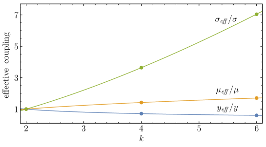
Figure 1: Numerical value of the effective inflaton matter-couplings $y_{{\rm{\it eff}}}$, $\mu_{{\rm{\it eff}}}$ and $\sigma_{{\rm{\it eff}}}$ normalized to their Lagrangian values $y$, $\mu$ and $\sigma$ respectively, as function of $k$. Here $m_{{\rm{\it eff}}}=0$.

The rates for the inflaton decay processes that we have introduced above, namely (3.2), (3.4) and (3.5), implicitly assume that the decay products of the inflaton are massless. However, as the oscillations of the inflaton provide a background in which $\phi$ acquires an effective mass, the same will occur for the decay products $f$ and $b$. The tree-level couplings of these fields to the inflaton lead to the following form for their time-dependent effective masses,

$$m_{{\rm{\it eff}}}^{2}(t)\;\equiv\;\begin{cases}y^{2}\phi^{2}\,,&\phi\rightarrow\bar{f}f\,,\\ 2\mu\phi\,,&\phi\rightarrow bb\,,\\ 2\sigma\phi^{2}\,,&\phi\phi\rightarrow bb\,.\end{cases}$$ (3.6)

Hence, the condition $m_{{\rm{\it eff}}}^{2}(t)\ll m_{\phi}^{2}$ for the efficient population of the relativistic plasma from inflaton decay is in general a time-dependent statement. At the perturbative level, disregarding the short time-scale of oscillations of $\phi$, the effect of this time-dependent effective mass can be determined upon averaging over the oscillations the effective decay rate. This procedure is discussed in detail in Appendix A. The parameter which determines the relevance of the induced mass is given by

$$\mathcal{R}(t)\;\equiv\;\frac{8}{\pi k^{2}\lambda}\left(\frac{\Gamma(\frac{1}{k})}{\Gamma(\frac{1}{2}+\frac{1}{k})}\right)^{2}\times\begin{cases}y^{2}\left(\dfrac{\phi_{0}(t)}{M_{P}}\right)^{4-k}\,,&\phi\rightarrow\bar{f}f\,,\\[9.0pt] 2\dfrac{\mu}{M_{P}}\left(\dfrac{\phi_{0}(t)}{M_{P}}\right)^{3-k}\,,&\phi\rightarrow bb\,,\\[9.0pt] 2\sigma\left(\dfrac{\phi_{0}(t)}{M_{P}}\right)^{4-k}\,,&\phi\phi\rightarrow bb\,.\end{cases}$$ (3.7)

Note that $\mathcal{R}\propto(m_{{\rm{\it eff}}}/m_{\phi})^{2}|_{\phi\rightarrow\phi_{0}}$. For $\mathcal{R}\ll 1$, the effective mass of the decay products is much smaller than the inflaton mass, and any kinematic effects can be safely disregarded. However, for $\mathcal{R}\gtrsim 1$, the phase-space dependence on $m_{{\rm{\it eff}}}$ must be taken into account. For the $\phi\rightarrow\bar{f}f$ and $\phi\phi\rightarrow bb$ cases, for which $m_{{\rm{\it eff}}}\propto\phi^{2}$, the result is a suppression of the mean decay rate of $\phi$. This kinematic blocking is, however, not total, as for any value of the coupling there will exist a time interval around the moment when $\phi=0$ during which the decay is allowed. A numerical evaluation of the corresponding phase-space factors reveals that $\Gamma_{\phi}\propto\mathcal{R}^{-1/2}$ when $\mathcal{R}\gg 1$ (see Appendix A). On the other hand, for $\phi\rightarrow bb$, $m_{{\rm{\it eff}}}\propto\phi$, and hence for half of the inflaton oscillation this effective mass becomes negative. Therefore on average not only there is no kinematic suppression in this scenario for $\mathcal{R}\gg 1$, but in fact there is an enhancement of the decay rate, $\Gamma_{\phi}\propto\mathcal{R}^{1/2}$ (see Fig. 11). This steep enhancement of the inflaton width is related to the tachyonic excitation of $b$, which signals the breakdown of the perturbative approximation and the need to consider the short-time preheating effects. In fact, the condition $\mathcal{R}\gg 1$ coincides, in all three cases, with the broad resonance regime, in which the non-perturbative production of non-relativistic decay products can be efficient [60, 61]. We will not consider this case in our work, and will be the subject of an independent analysis.

As one can see from (3.7), depending on the value of $k$ and the primary mode for decay (or scattering), the ratios in (3.7) will scale as $\phi_{0}^{p}$ where $p$ may be positive or negative. As we are implicitly assuming that the inflaton is evolving from an initially large value to the origin, the ratios in (3.7) may either increase or decrease. Consider for example that inflaton decay has a dominant fermionic decay channel (or if the depletion of the inflaton is dominated by $\phi\phi\rightarrow bb$). In this case $\mathcal{R}$ decreases for $k<4$. Therefore, if inflaton decay is not kinematically suppressed when inflation ends at $t=t_{\rm end}$, it will also not be suppressed at any subsequent time. If at $t=t_{\rm end}$ the decay is suppressed, the efficient decay of $\phi$ is delayed until $\phi_{0}(t)$ decreases sufficiently to allow the decay. For $k>4$, the mass ratio (3.7) increases with decreasing $\phi_{0}$ in these channels and even if decay is possible at $t=t_{\rm end}$, it becomes blocked at later times. For boson dominated decays, these qualitative effects depend on $p>{\rm or}<3$. However, in this case instead of a decrease in the efficiency of the decay, we observe the breakdown of the perturbative approximation due to an increase in the rate. We comment on this further in the discussion section.

Fig. 2 shows the evolution of the mass ratio $\mathcal{R}$ for the case of inflaton decays into fermions and bosons, for $k=2,4,6$ as function of $\frac{a}{a_{\mathrm{end}}}$, where $a_{\rm end}=a(t_{\rm end})$ denotes the scale factor at the end of inflation. For fermions, shown in the left panel, we find, as expected, that $\mathcal{R}$ decreases for $k<4$, is constant for $k=4$ and increases for $k>4$. For the chosen value of $y$, the effect of the kinematic suppression for $k\leq 4$ can be neglected. However, for $k=6$, the decay quickly becomes kinematically blocked, resulting in a reduced decay rate. This reflects the fact that for large values of $k$, the inflaton mass (3.3) redshifts faster than that of the decay product masses (3.6) which are independent of $k$. For reference, the delay of inflaton-radiation equality would lead to a reheating temperature $T_{\rm RH}\simeq 4\times 10^{-17}\,{\rm GeV}$, lower than the present photon temperature and in clear conflict with cosmological constraints including big bang nucleosynthesis [62, 63]. On the other hand, for the bosonic decay channel, we observe that $\mathcal{R}$ decreases for $k=2$, but it rapidly increases for $k=4,6$. This results in a shortened reheating epoch. We can then conclude that the shape of the inflationary potential about the origin as determined by the value of $k$ has a strong effect on the kinematics of the final state, in addition to its effect on the inflaton width. We are now in a position to analyze the evolution of the temperature of the thermal bath produced by inflaton decay and scattering.

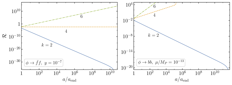
Figure 2: The kinematic parameter $\mathcal{R}$ defined in (3.7) for fermionic (left) and bosonic (right) decays of the inflaton, as a function of the scale factor for $k=2,4,6$. T-attractor values are chosen for the potential parameter $\lambda$ and the inflaton $\phi_{\rm end}$ (see Appendix B). Inflaton-radiation equality occurs at $a_{\rm RH}/a_{\rm end}\simeq 10^{10}\,(2\times 10^{11}),\,7\times 10^{14}\,(10^{5})$ and $2\times 10^{28}\,(4\times 10^{3})$ for fermions (bosons) with $k=2,4,6$, respectively.

4 The Reheating Process

We use Eqs. (2.12), (2.14), and (2.15) to determine the time evolution of the energy density of the decay products of the inflaton during reheating. We can write the dissipation rate in terms of $\rho_{\phi}$ to obtain a closed set of evolution equations. If we average over several oscillations and combine Eqs. (3.2), (3.3), (3.4) and (3.5), we have

$$\Gamma_{\phi}(t)\;=\;\gamma_{\phi}\left(\frac{\rho_{\phi}}{M_{P}^{4}}\right)^{l}\,,$$ (4.1)

where

$$\gamma_{\phi}\;=\;\begin{cases}\sqrt{k(k-1)}\lambda^{1/k}M_{P}\dfrac{y_{{\rm{\it eff}}}^{2}}{8\pi}\,,\quad&\phi\rightarrow\bar{f}f\,,\\[10.0pt] \dfrac{\mu_{{\rm{\it eff}}}^{2}}{8\pi\sqrt{k(k-1)}\lambda^{1/k}M_{P}}\,,\quad&\phi\rightarrow bb\,,\\[10.0pt] \dfrac{\sigma_{{\rm{\it eff}}}^{2}M_{P}}{8\pi[k(k-1)]^{3/2}\lambda^{3/k}}\,,\quad&\phi\phi\rightarrow bb\,,\end{cases}$$ (4.2)

and

$$l\;=\;\begin{cases}\frac{1}{2}-\frac{1}{k}\,,\quad&\phi\rightarrow\bar{f}f\,,\\ \frac{1}{k}-\frac{1}{2}\,,\quad&\phi\rightarrow bb\,,\\ \frac{3}{k}-\frac{1}{2}\,,\quad&\phi\phi\rightarrow bb\,.\end{cases}$$ (4.3)

Multiplying both sides of Eq. (2.12) by $a^{\frac{6k}{k+2}}$, replacing $\Gamma_{\phi}$ by (4.1), replacing $w_{\phi}$ using Eq. (2.13), and replacing the dynamical parameter $t$ by $a$ with $\frac{d}{dt}=aH\frac{d}{da}$ we obtain

$$\frac{d}{da}\left(\rho_{\phi}a^{\frac{6k}{k+2}}\right)=-\frac{\gamma_{\phi}}{aH}\frac{2k}{k+2}\frac{\rho_{\phi}^{l+1}}{M_{P}^{4l}}a^{\frac{6k}{k+2}}\,.$$ (4.4)

If we now suppose $\gamma_{\phi}\ll H$, valid at early times,

$$\rho_{\phi}(a)=\rho_{\rm end}\left(\frac{a}{a_{\rm end}}\right)^{-\frac{6k}{k+2}}\,,$$ (4.5)

where $\rho_{\rm end}=\rho_{\phi}(a_{\rm end})$. At later times, for $k=2$, $\rho_{\phi}\propto e^{-\Gamma_{\phi}t}$, however, the decay of the inflaton is not exponential for $k>2$.

Inserting Eq. (4.5) into (2.14) and performing a similar manipulation, we have

$$\frac{1}{a^{4}}\frac{d}{da}\left(\rho_{R}a^{4}\right)\;=\;\frac{2k}{k+2}\frac{\gamma_{\phi}}{aH}\frac{\rho_{\phi}^{l+1}}{M_{P}^{4l}}\,.$$ (4.6)

This expression is easily integrated to give

$$\rho_{R}\;=\;\frac{2k}{k+8-6kl}\frac{\gamma_{\phi}}{H_{\rm end}}\frac{\rho_{\rm end}^{l+1}}{M_{P}^{4l}}\left(\frac{a_{\rm end}}{a}\right)^{4}\left[\left(\frac{a}{a_{\rm end}}\right)^{\frac{k+8-6kl}{k+2}}-1\right]\,,$$ (4.7)

where $H^{2}_{\rm end}=\rho_{\rm end}/3M_{P}^{2}$. At later times when $a\gg a_{\rm end}$ and $8+k-6kl>0$, we can approximate $\rho_{R}$ as

$$\rho_{R}^{a\gg a_{\rm end}}\;=\;\frac{2k}{k+8-6kl}\frac{\gamma_{\phi}}{H_{\rm end}}\frac{\rho_{\rm end}^{l+1}}{M_{P}^{4l}}\left(\frac{a_{\rm end}}{a}\right)^{\frac{3k+6kl}{k+2}}\,.$$ (4.8)

For the case with dominant inflaton decays to fermions, $\phi\to f\bar{f}$, when $l=(k-2)/2k$, we recover the result in Ref. [9] .

Given the expression for $\rho_{R}$ in Eq. (4.7), the temperature of the radiation bath is simply

$$\rho_{R}=\frac{g_{\rho}\pi^{2}}{30}T^{4}~{}~{}~{}~{}\Rightarrow~{}~{}~{}~{}T=\left(\frac{30\rho_{R}}{g_{\rho}\pi^{2}}\right)^{\frac{1}{4}}\propto a^{-\frac{3k+6kl}{4k+8}}\,,$$ (4.9)

where $g_{\rho}$ is the number of relativistic degrees of freedom at temperature $T$. Note that if $8+k-6kl<0$,

$$\rho_{R}^{a\gg a_{\rm end}}\;=\;\frac{2k}{6kl-k-8}\frac{\gamma_{\phi}}{H_{\rm end}}\frac{\rho_{\rm end}^{l+1}}{M_{P}^{4l}}\left(\frac{a_{\rm end}}{a}\right)^{4}\,,$$ (4.10)

which implies that the temperature would simply redshift as $T\propto a^{-1}$. As a summary, we provide in Table 1 the dependence of $T$ as function of $a$ for the different cases we analyze in our work. In the last column of the table, we show the form of the temperature evolution when ${\cal R}\gg 1$.

channel	generic	$k=2$	$k=4$	$k=6$	$m^{2}_{{\rm{\it eff}}}\gg m^{2}_{\phi}$
$\phi\rightarrow\bar{f}f$	$T\propto a^{-\frac{3k-3}{2k+4}}$	$T\propto a^{-3/8}$	$T\propto a^{-3/4}$	$T\propto a^{-15/16}$	$T\propto a^{-\frac{9(k-2)}{4(k+2)}}$
$\phi\rightarrow bb$	$T\propto a^{-\frac{3}{2k+4}}$	$T\propto a^{-3/8}$	$T\propto a^{-1/4}$	$T\propto a^{-3/16}$	$T\propto a^{-\frac{3(5-k)}{4(k+2)}}$
$\phi\phi\rightarrow bb$	$T\propto a^{-\frac{9}{2k+4}}$	$T\propto a^{-1}$	$T\propto a^{-3/4}$	$T\propto a^{-9/16}$	$T\propto a^{-3/4}$

Table 1: Dependence of the temperature $T$ as function of the scale factor $a$ for the different cases we analyze in this work. The ‘generic’ result assumes the validity of Eq. (4.8). In the last column non-perturbative particle production has not been taken into account, even if $\mathcal{R}\gg 1$.

At the end of inflation, before inflatons decay, $\rho_{R}=0$ and hence $T=0$. The Universe begins to reheat and a maximum temperature is attained before the temperature begins to fall off as given in Table 1. The maximum temperature can be computed from Eq.(4.7). From $\frac{d\rho_{R}}{da}=0$, we obtain

$$a_{\rm max}=a_{\rm end}\left(\frac{4k+8}{3k+6kl}\right)^{\frac{k+2}{k+8-6kl}}\,,$$ (4.11)

which gives

$$\rho_{R}^{\rm max}\;=\;\frac{2}{3+6l}\frac{\gamma_{\phi}}{H_{\rm end}}\frac{\rho_{\rm end}^{l+1}}{M_{P}^{4l}}\left(\frac{4k+8}{3k+6kl}\right)^{-\frac{4k+8}{k+8-6kl}}\,,$$ (4.12)

and

$$T_{\rm max}=\left(\frac{30}{g_{\rho}\pi^{2}}\rho_{R}^{\rm max}\right)^{\frac{1}{4}}.$$ (4.13)

We show in Figs. 3 and 4 the evolution of the temperature obtained by numerically solving Eqs. (2.12)-(2.15), as function of the scale factor $a/a_{\rm end}$ for two choices of $k=2$ and 4. To see the effect of the kinematic suppression, we compare the results where $m_{{\rm{\it eff}}}$ is given by Eq. (3.6) to one where we set $m_{{\rm{\it eff}}}=0$. We begin by considering the case with $k=2$. The value $\phi_{\rm end}$ is determined by the condition that exponential expansion ceases, or $\ddot{a}=0$. The scale of the potential, $\lambda$ can be obtained by the normalization of the CMB and the number of $e$-folds since horizon crossing. This procedure is worked out for the T-attractor models in Appendix B. For $k=2$ we find $\lambda=2.5\times 10^{-11}$ and $\rho_{\rm end}^{1/4}=5.2\times 10^{15}$ GeV. Since we expect the evolution of the temperature to be similar for the cases of decays to bosons and fermions (see Table 1), we include only decays to fermions and annihilations to boson pairs. In Fig. 3, we take $y=\sigma=10^{-7}$ (left) and $y=10^{-7}$ and $\sigma=10^{-9}$ (right). For inflaton decays to fermions, we can estimate the maximum temperature attained from Eqs. (4.12) and (4.13),

$$\rho_{R}^{\rm max}=\frac{\sqrt{6}}{32\pi}\left(\frac{3}{8}\right)^{3/5}~{}y^{2}M_{P}^{2}\left(\lambda\rho_{\rm end}\right)^{\frac{1}{2}}~{}~{}~{}\Rightarrow~{}~{}~{}T_{\rm max}\sim 2\times 10^{11}\left(\frac{y}{10^{-7}}\right)^{1/2}~{}\rm{GeV},$$ (4.14)

in good agreement with the numerical result shown in the figure. Similarly, for annihilations to boson pairs, we expect

$$\rho_{R}^{\rm max}=\frac{\sqrt{3/2}}{72\pi M_{P}^{2}}\left(\frac{8}{9}\right)^{8}~{}\sigma^{2}\lambda^{-\frac{3}{2}}\left(\rho_{\rm end}\right)^{\frac{3}{2}}~{}~{}~{}\Rightarrow~{}~{}~{}T_{\rm max}\sim 6\times 10^{12}\left(\frac{\sigma}{10^{-9}}\right)^{1/2}~{}\rm{GeV},$$ (4.15)

which is close to the result shown in the figure for the case where the kinematic suppression in the final state is ignored (the dotted curves with $m_{{\rm{\it eff}}}=0$).

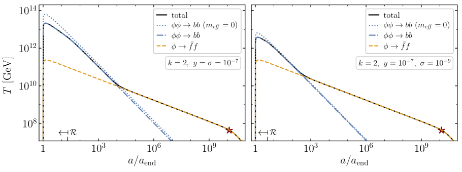
Figure 3: Evolution of the instantaneous temperature during reheating for $k=2$ in the case of inflaton decays to fermions (dashed, orange) and annihilations to bosons (blue). In the latter, we show separately the case when the effective masses of the decay products are ignored (dotted) and included (dot dashed). The case of both decays and annihilations (with effective masses included) is also shown (solid, black). In the left panel we take $y=\sigma=10^{-7}$ and in the right panel $y=10^{-7}$ and $\sigma=10^{-9}$. Here $\rho_{\rm end}=(5.2\times 10^{15}\,{\rm GeV})^{4}$ and $\lambda=2.5\times 10^{-11}$, assuming T-attractor inflation boundary conditions. The star signals inflation-radiation equality. The arrow points toward the region where $\mathcal{R}>1$ for one or more of the decay channels.

Also apparent in Fig. 3 is the difference in the slopes of the evolution, $T\propto a^{-3/8}$ for decays to fermions, and $T\propto a^{-1}$, for annihilations to bosons (see again Table 1). We can estimate the value of $a/a_{\rm end}$ for which the two contributions are equal by using Eqs. (4.8) and (4.10), and we obtain

$$\rho^{f}_{R}=\rho^{b}_{R}~{}\Rightarrow~{}~{}\left(\frac{a}{a_{\rm end}}\right)=\left(\frac{5}{4}\frac{\rho_{\rm end}}{M_{P}^{4}}\frac{\sigma^{2}}{y^{2}\lambda^{2}}\right)^{2/5}\simeq 18000~{}~{}\rm{for}~{}\sigma={10^{-7}}~{}\rm{and}~{}\simeq 450~{}\rm{for}~{}\sigma=10^{-9}.$$ (4.16)

This is in reasonable agreement with the numerical result in Fig. 3. For the value of $y$ adopted in Fig. 3, the value of $\mathcal{R}$ in Eq. (3.7) is much smaller than one, and we do not expect (and do not find) any kinematic suppression for the evolution of $T$ produced by decays to fermions. In contrast, we do find some suppression for the case of inflaton annihilations to bosons. This is evidenced by the suppression in $T_{\rm max}$ and the change in slope in the blue dot-dashed curve when compared with the dotted curve for which the effect is neglected. We can estimate the value of $a$ for which the change in slope occurs from the condition $\mathcal{R}\simeq 1$. For $k=2$, we find

$$\mathcal{R}=\frac{4\sigma\rho_{\rm end}}{\lambda^{2}M_{P}^{4}}\left(\frac{a_{\rm end}}{a}\right)^{3}\simeq 1\ \ \Rightarrow\ \ a\simeq 20~{}\left(\sigma/10^{-7}\right)^{1/3}~{}a_{\rm end}\,,$$ (4.17)

where we have used Eq. (4.5) and $\rho_{\phi}=V(\phi_{0})$, Eq. (2.10). Once again, our analytic approximation is in good agreement with the position of the change in slope seen in Fig. 3. Finally, as noted earlier, the effect of the kinematic suppression causes an effective reduction of the decay rate by $\mathcal{R}^{-1/2}$ when $\mathcal{R}>1$. For $l=\frac{3}{k}-\frac{1}{2}$ (the value corresponding to the process $\phi\phi\rightarrow bb$), $\mathcal{R}^{-1/2}\sim a^{(12-3k)/(k+2)}$ and integrating Eq. (4.6) with $\gamma_{\phi}\to\gamma_{\phi}\mathcal{R}^{-1/2}$, we find $T\sim a^{-3/4}$ for all values of $k$ when kinematic suppression is important, and $T\sim a^{-1}$ at later times, when the suppression is no longer important as seen in Fig. 3. Note also the change in slope at $\left(\frac{a}{a_{\rm end}}\right)\simeq 10^{10}$, where $T$ becomes proportional to $a^{-1}$, corresponding to the reheat temperature $T=T_{\rm RH}$ defined by $\rho_{\phi}=\rho_{R}$ and discussed in more detail below.

We next consider the evolution of the temperature for the case with $k=4$. In this case, the evolution of the temperature due to annihilations to bosons is similar to that from decays to fermions, and we ignore inflaton annihilations by setting $\sigma=0$. In Fig. 4, we compare the evolution of the temperature for two choices of the fermionic coupling, $y=10^{-6}$ (left) and $y=3\times 10^{-8}$ (right) for a common coupling to bosons, $\mu=10^{-13}M_{P}$. From the normalizations derived in Appendix B, we now find $\lambda=3.3\times 10^{-12}$ and $\rho_{\rm end}^{1/4}=4.8\times 10^{15}\,{\rm GeV}$. From Eqs. (4.12) and (4.13), we find

$$\rho_{R}^{\rm max}=\frac{27}{256\pi}~{}y^{2}_{{\rm{\it eff}}}M_{P}\lambda^{\frac{1}{4}}\rho_{\rm end}^{\frac{3}{4}}~{}~{}~{}\Rightarrow~{}~{}~{}T_{\rm max}\sim 6\times 10^{11}\left(\frac{y}{10^{-6}}\right)^{1/2}~{}\rm{GeV},$$ (4.18)

for our assumed values of $\lambda$, and $\rho_{\rm end}$ with $g_{\rho}\sim 100$. This is very close to the maximum temperature attained in the numerical result shown in Fig. 4. For $y=10^{-6}$, we see that the initial stages of reheating are dominated by fermionic final states, and the temperature evolution is governed by $T\propto a^{-3/4}$ as expected from Eq. (4.9), until decays to bosons become important. Decays to bosons lead to a maximum temperature given by

$$\rho_{R}^{\rm max}=\frac{\mu^{2}_{{\rm{\it eff}}}}{12\pi}4^{-\frac{4}{3}}\lambda^{-\frac{1}{4}}M_{P}\rho_{\rm end}^{\frac{1}{4}}~{}~{}\Rightarrow~{}~{}~{}T_{\rm max}\simeq 10^{11}\left(\frac{\mu}{10^{-13}M_{P}}\right)^{1/2}~{}\rm{GeV}.$$ (4.19)

However the temperature produced from decays to bosons falls off slower, as $T\propto a^{-1/4}$ and bosonic reheating dominates when

$$\frac{a}{a_{\rm end}}\;=\;6\frac{y_{{\rm{\it eff}}}}{\mu_{{\rm{\it eff}}}}\left(\lambda\rho_{\rm end}\right)^{1/4}\;\simeq\;80\,,$$ (4.20)

from Eq.(4.8) for $y=10^{-6}$ and $\mu=10^{-13}M_{P}$. This corresponds to what we obtained numerically in Fig. 4.

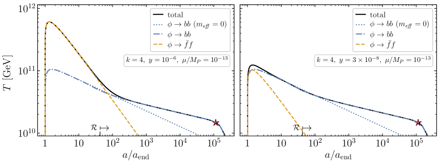
Figure 4: Evolution of the instantaneous temperature during reheating for $k=4$ in the case of inflaton decays to fermions (dashed, orange), bosons (blue). In the latter, we show separately the case when the effective masses of the decay products are ignored (dotted) and included (dot dashed). The case of both decays and annihilations (with effective masses included) is also shown (solid, black). In both cases the bosonic coupling is fixed to $\mu=10^{-13}\,M_{P}$. The left panel depicts $T$ vs. $a$ for $y=10^{-6}$. The right panel corresponds to $y=3\times 10^{-8}$. Here $\rho_{\rm end}=(4.8\times 10^{15}\,{\rm GeV})^{4}$ and $\lambda=3.3\times 10^{-12}$, assuming T-attractor inflation boundary conditions. The star signals inflation-radiation equality. The arrow points toward the region where $\mathcal{R}>1$ for one or more of the decay channels.

For larger values of $a$, the bosonic gas, even if less populated at the beginning of reheating, because of our choices of $y_{{\rm{\it eff}}}$ and $\mu_{{\rm{\it eff}}}$, begins to dominate the energy budget of the thermal bath. This comes from the fact the whereas the production rate of fermions decreases with $\phi_{0}$ (Eq. 3.2), the opposite is true for the process $\phi\rightarrow bb$ which becomes more efficient with time (Eq. 3.4). This is reflected in the temperature evolution, $T\propto a^{-3/4}$ for the fermionic plasma and $T\propto a^{-1/4}$ for a bosonic plasma (see Table 1). On the other hand, if we set $y_{{\rm{\it eff}}}=\frac{\mu_{{\rm{\it eff}}}}{m_{\phi}}=3\times 10^{-8}$ for $\mu=10^{-13}M_{P}$ as illustrated in Fig. 4 (right), we will obtain roughly the same amount of fermionic and bosonic components at $T_{\rm max}$, but because the temperature evolves differently for the two species, only the bosonic final states reheat the Universe.

The value of $a$ for which the bosonic enhancement factor ${\cal R}$ plays a significant role is given by ${\cal R}\gtrsim 1$, or

$${\cal R}=\frac{\mu}{\lambda^{3/4}\pi\rho_{\rm end}^{1/4}}\left[\frac{\Gamma(\frac{1}{4})}{\Gamma(\frac{3}{4})}\right]^{2}\left(\frac{a}{a_{\rm end}}\right)\gtrsim 1\quad\ \Rightarrow\quad\ a\gtrsim 20\,a_{\rm end}\,.$$ (4.21)

The numerical result shows that the slope change occurs around $a/a_{\rm end}\sim 100$, indicating the effect of the enhancement requires ${\cal R}\sim 5$ (see Appendix A.2). At large $a$, when the enhancement is effective, the slope changes from $T\propto a^{-1/4}$ to $T\propto a^{-1/8}$, corresponding to the shallow slope seen in Fig. 4. It must be emphasized that a significant amount of uncertainty is present, since we have neglected non-perturbative particle production.

When we decrease $y$ so that the value of $T_{\rm max}$ produced by decays to fermions is approximately equal to that as decays to bosons as in Fig. 4 (right), we observe that, as expected, the reheating is first dominated by the process $\phi\rightarrow bb$. In the absence of kinematic blocking, the temperature of the plasma due to final state bosons falls off as $T\sim a^{-1/4}$ until the end of reheating (when $t\simeq\Gamma_{\phi}^{-1}$). However, kinematic enhancement turns on at $a\simeq 100~{}a_{\rm end}$ and the temperature falls off more gradually as $T\sim a^{-1/8}$ until the radiation bath dominates the energy density at $a_{\rm RH}\simeq 10^{5}~{}a_{\rm end}$ which we define as the moment of reheating and subsequently $T\sim a^{-1}$ as discussed further in the next subsection.

As we have seen in the previous subsection, reheating is a continuous process as inflaton decays products appear and thermalize. We define the reheat temperature when

$$\rho_{R}(T_{\rm RH})=\rho_{\phi}(T_{\rm RH})$$ (4.22)

which gives, using Eqs. (4.5) and (4.8)

$$\frac{a_{\rm RH}}{a_{\rm end}}=\left[\frac{k+8-6kl}{2k}\frac{M_{P}^{4l-1}\rho_{\rm end}^{\frac{1}{2}-l}}{\sqrt{3}\gamma_{\phi}}\right]^{\frac{k+2}{3k-6kl}}\,,$$ (4.23)

for $8+k-6kl>0$. For $8+k-6kl<0$, we can use Eq. (4.10) to obtain,

$$\frac{a_{\rm RH}}{a_{\rm end}}=\left[\frac{6kl-k-8}{2k}\frac{M_{P}^{4l-1}\rho_{\rm end}^{\frac{1}{2}-l}}{\sqrt{3}\gamma_{\phi}}\right]^{\frac{k+2}{2k-8}}\,.$$ (4.24)

Note that Eq. (4.24) is only true for $k>4$. When $k\leq 4$ and $8+k-6kl<0$, reheating never occurs. Consider for example the case for $\phi\phi\to bb$. In Eq. (4.24), we would find $a_{\rm RH}<a_{\rm end}$ which is clearly unphysical. Indeed, from Table 1, for $k=2$ we infer that $\rho_{R}\sim a^{-4}$ while $\rho_{\phi}\sim a^{-3}$. For this case even for $k=4$, $\rho_{R}$ never comes to dominate the energy density in the absence of other inflaton-matter couplings.

For $k=2$, inflaton decays to fermions dominate at late times with respect to scatterings to bosons, and $l=0$, so that $\frac{a_{RH}}{a_{\rm end}}\sim 1.8\times 10^{10}$ taking the parameter values used in Fig. 3. Furthermore, for $y=10^{-7}$, ${\cal R}<1$ initially, and for $k=2$, it remains so, the reheat temperature is not affected by the fermionic suppression. For $k=4$, boson final states dominate at late times, $l=-1/4$, and from the parameters used in Fig. 4 we obtain $\frac{a_{RH}}{a_{\rm end}}=4\times 10^{5}$. However, a more precise calculation should take into account the change in the slope of $\rho_{R}$ due to the kinematic enhancement when $\mathcal{R}>1$. In this case, we obtain

$$\rho_{R}=\frac{\mu_{{\rm{\it eff}}}^{2}M_{P}\rho_{\rm end}^{\frac{1}{4}}}{36\pi\lambda^{\frac{1}{4}}}\left(\frac{a_{\rm end}}{a_{\cal R}}\right)\left(\frac{a_{\cal R}}{a}\right)^{\frac{1}{2}},$$ (4.25)

where $a_{\cal R}$ is the scale factor from which the boosted enhancement begins to have significant effect, computed in Eq.(4.21) (that is, $a=a_{\cal R}$ when ${\cal R}=1$). Then the scale factor at reheating determined by $\rho_{R}=\rho_{\phi}$ is

$$\frac{a_{\rm RH}}{a_{\rm end}}=\left[\sqrt{\frac{a_{\cal R}}{a_{\rm end}}}\frac{36\pi\lambda^{\frac{1}{4}}\rho_{\rm end}^{\frac{3}{4}}}{\mu_{{\rm{\it eff}}}^{2}M_{P}}\right]^{\frac{2}{7}}\sim 10^{5},$$ (4.26)

where we used Eq. (4.21) for $\frac{a_{\cal R}}{a_{\rm end}}$. This result is in good agreement with Fig. 4.

When ${\cal R}<1$, it is relatively straight forward to use the expressions for $a_{\rm RH}$ to determine the reheating temperature:

$$T_{\rm RH}\; =\;\left(\frac{30}{g_{\rho}\pi^{2}}\right)^{\frac{1}{4}}\left[\frac{2k}{k+8-6kl}\frac{\sqrt{3}\gamma_{\phi}}{M_{P}^{4l-1}}\right]^{\frac{1}{2-4l}}$$ (4.27)

for $8+k-6kl>0$. For $8+k-6kl<0$ and $k>4$,

$$T_{\rm RH}\; =\;\left(\frac{30}{g_{\rho}\pi^{2}}\right)^{\frac{1}{4}}\left[\frac{2k}{6kl-k-8}\frac{\sqrt{3}\gamma_{\phi}}{M_{P}^{4l-1}}\rho_{\rm end}^{\frac{6kl-k-8}{6k}}\right]^{\frac{3k}{4k-16}}\,.$$ (4.28)

For the particular case depicted in Fig. 3, for $\phi\rightarrow\bar{f}f$, $l=\frac{1}{2}-\frac{1}{k}$, and we have

$$T_{\rm RH}^{f}=\left(\frac{30}{g_{\rho}\pi^{2}}\right)^{\frac{1}{4}}\left[\frac{k\sqrt{3k(k-1)}}{7-k}\lambda^{\frac{1}{k}}\frac{y^{2}}{8\pi}\right]^{\frac{k}{4}}M_{P}\,,$$ (4.29)

and for the parameters used in Fig. 3 and $g_{\rho}\sim 100$, $T_{\rm RH}\simeq 4.4\times 10^{7}$ GeV. For decays to bosons, $\phi\rightarrow bb$, $l=\frac{1}{k}-\frac{1}{2}$, and we include the enhancement factor proportional to ${\cal R}^{1/2}$ (which applies for $k>3$) and find

$$T_{\rm RH}^{b}=\left(\frac{30}{g_{\rho}\pi^{2}}\right)^{\frac{1}{4}}\left[\frac{1}{7\pi^{3/2}}\sqrt{\frac{3}{k(k-1)^{3}}}\frac{\Gamma(\frac{1}{k})}{\Gamma(\frac{1}{2}+\frac{1}{k})}\left(\frac{\mu}{\lambda^{1/k}M_{P}}\right)^{5/2}\left(\frac{\mu_{{\rm{\it eff}}}}{\mu}\right)^{2}\right]^{\frac{k}{6k-10}}M_{P}\,.$$ (4.30)

When evaluated with the parameters used in Fig. 4, for $k=4$, we have $T_{\rm RH}=2\times 10^{10}$ GeV. Eqs. (4.29) and (4.30) are two solutions for $T_{\rm RH}$ corresponding to cases considered in the examples in Figs. (3) and (4). There are of course several other possible expressions for $T_{\rm RH}$ depending on the kinematic factor ${\cal R}$. When ${\cal R}>1$, we must modify the integrand used to determine Eq. (4.7) as well as the limits of integration if ${\cal R}$ evolves in such a way that it crosses ${\cal R}=1$ between $a_{\rm end}$ and $a_{\rm RH}$.

5 Dark matter production

As noted earlier, it is possible to produce certain very weakly interacting dark matter candidates during the reheating process. The relic abundance of these dark matter candidates may depend primarily on $T_{\rm max}$, $T_{\rm RH}$, or both depending on the production cross section. We parametrize the thermally-averaged effective cross section for dark matter (DM) production in the following way,

$$\langle\sigma v\rangle\;=\;\frac{T^{n}}{{\tilde{\Lambda}}^{n+2}}\,,$$ (5.1)

where the mass scale ${\tilde{\Lambda}}$ is assumed to be parametrically related to the mass of a heavy mediator in the UV theory. For $n>-1$, DM production after reheating is subdominant [40, 7, 15, 64]. For example, in the case of a weak scale gravitino, $n=0$, and ${\tilde{\Lambda}}\propto M_{P}$. In contrast, in high scale supersymmetry, $n=6$, and ${\tilde{\Lambda}}^{2}\propto m_{3/2}M_{P}$. It is worth emphasizing that this effective description is valid as long as ${\tilde{\Lambda}}$ is above $T_{\rm max}$. The amount of DM produced during reheating is obtained from the solution of the following Boltzmann equation,

$$\dot{n}_{\chi}+3Hn_{\chi}\;=\;g_{\chi}^{2}\langle\sigma v\rangle n_{r}^{2}\;\equiv\;R(T)\,,$$ (5.2)

where $g_{\chi}$ denotes the number of internal degrees of freedom of the DM particle $\chi$, and $n_{R}$ corresponds to the number density of the radiation, which in equilibrium can be written as

$$n_{R}\;=\;\frac{\zeta(3)}{\pi^{2}}T^{3}\,.$$ (5.3)

The production rate per unit volume can be written as

$$R(T)=\frac{T^{n+6}}{\Lambda^{n+2}}\,,$$ (5.4)

where we have absorbed the numerical factors in $\Lambda^{n+2}={\tilde{\Lambda}}^{n+2}\pi^{4}/g_{\chi}^{2}\zeta(3)^{2}$.

Assuming instantaneous thermalization, it is convenient to define the DM yield as $Y_{\chi}\equiv n_{\chi}/T^{\frac{(4k+8)}{(k+2kl)}}$, where the power of $T$ is inferred from Eq. (4.9) with $Y_{\chi}\sim n_{\chi}a^{3}$. The Boltzmann equation (5.2) can be rewritten as

$$\frac{dY_{\chi}}{dT}=-\frac{R(T)}{H(T)}\left(\frac{4k+8}{3k+6kl}\right)T^{-\frac{5k+8+2kl}{k+2kl}}\,,$$ (5.5)

(if $8+k-6kl>0$). Furthermore, we can write $H(T)$ (which we assume is dominated by $\rho_{\phi}$) in terms of $T_{\rm RH}$ by noting that at $T_{\rm RH}$, $\rho_{\phi}=\rho_{R}$ and that $\rho_{R}(T_{\rm RH})=\alpha T_{\rm RH}^{4}$, where $\alpha=g_{\rho}\pi^{2}/30$. Using the scaling of $\rho_{\phi}$ with $a$ from Eq. (4.5), and the scaling of $a$ with $T$ from Eq. (4.9), we can write

$$H=\sqrt{\frac{\alpha}{3}}\frac{T_{\rm RH}^{2}}{M_{P}}\left(\frac{T}{T_{\rm RH}}\right)^{\frac{4}{1+2l}}\,$$ (5.6)

which is interestingly independent of $k$ (except for the implicit $k$ dependence in $l$).

We are now in a position to integrate Eq. (5.5)

$$Y_{\chi}(T_{\rm RH})=\sqrt{\frac{3}{\alpha}}\frac{M_{P}T_{\rm RH}^{\frac{2-4l}{1+2l}}}{\Lambda^{n+2}}\left(\frac{4k+8}{3k+6kl}\right)\int_{T_{\rm max}}^{T_{\rm RH}}dT\,T^{n+6}T^{-\frac{4}{1+2l}}T^{-\frac{5k+8+2kl}{k+2kl}}\,,$$ (5.7)

which is easily integrated to give

$$n_{\chi}(T_{\rm RH})\;\simeq\;\sqrt{\dfrac{1}{3\alpha}}M_{P}\begin{cases}\left(\dfrac{4k+8}{8+2k-12kl-kn-2kln}\right)\dfrac{T_{\rm RH}^{n+4}}{\Lambda^{n+2}}\,,&n<\dfrac{8+2k-12kl}{k(1+2l)}\,,\\[10.0pt] \left(\dfrac{4k+8}{k+2kl}\right)\dfrac{T_{\rm RH}^{n+4}}{\Lambda^{n+2}}\ln\left(\dfrac{T_{\rm max}}{T_{\rm RH}}\right)\,,&n=\dfrac{8+2k-12kl}{k(1+2l)}\,,\\[10.0pt] \left(\dfrac{4k+8}{12kl+kn+2kln-8-2k}\right)\left(\dfrac{T_{\rm RH}}{T_{\rm max}}\right)^{\frac{8+6k-4kl}{k+2kl}}\dfrac{T_{\rm max}^{n+4}}{\Lambda^{n+2}}\,,&n>\dfrac{8+2k-12kl}{k(1+2l)}\,.\end{cases}$$ (5.8)

For $l\to(k-2)/2k$ as in the first line of Eq. (4.3) for fermionic final stats, these equations reduce to those in [9]. If we further specify $k=2$, they reduce to the results in [7, 51]. Note that aside from the prefactor, when $n\leq\frac{8+2k-12kl}{k(1+2l)}$, the abundance scales as $T_{\rm RH}^{n+4}$, ie., independent of $k$ and $l$. Only for larger $n$, does the power of $\frac{T_{\rm RH}}{T_{\rm max}}$ depend on $k$ and $l$. Though one should bear in mind that both $T_{\rm RH}$ and $T_{\rm max}$ each depend on $k$ and $l$ as discussed in the previous section.

Finally, the dark matter number density produced by scatterings in the thermal plasma given in Eqs. (5.8) can be converted to the dark matter contribution to the critical density using

$$\Omega_{\chi}h^{2}\; =\;\frac{m_{\chi}n(T_{0})}{\rho_{c}h^{-2}}$$

$$=\;\frac{\pi^{2}g_{\rho}(T_{0})m_{\chi}n_{\gamma}(T_{0})n_{\chi}(T_{\rm RH})}{2\zeta(3)g_{\rho}(T_{\rm RH})T_{\rm RH}^{3}\rho_{c}h^{-2}}$$

$$=\;5.9\times 10^{6}{\rm GeV}^{-1}\frac{m_{\rm DM}n_{\chi}(T_{\rm RH})}{T_{\rm RH}^{3}}\,,$$ (5.9)

where $g_{\rho}(T_{0})=43/11$ is the present number of effective relativistic degrees of freedom for the entropy density, $n_{\gamma}(T_{0})\simeq 410.66\,{\rm cm}^{-3}$ is the number density of CMB photons, and $\rho_{c}h^{-2}\simeq 1.0534\times 10^{-5}{\rm GeV\,cm}^{-3}$ is the critical density of the Universe. We consider for definiteness the high-temperature Standard Model value $g_{\rm RH}=427/4$.

Of course it is also possible that if the dark matter is coupled to the inflaton, that it may be produced directly in the decay process [40, 7, 6, 9]. However, as we have seen, the decay to dark matter may be suppressed, if the dark matter is fermionic, or enhanced if bosonic. To fully treat the production of dark matter through decay, we would need to specify separately a value of $l_{\chi}$ for the dark matter which may in principle differ from that of the standard model decay products involved in reheating. This is beyond the scope of the present work. Furthermore, even if the dark matter is not directly coupled to the inflaton, but is coupled to the standard model, the production of dark matter through direct decays may still proceed through loops [51], further complicating the calculation of the dark matter abundance. We save this study for future work.

6 An example: the SUSY case

The general reheating formalism that we have developed in the previous sections can be applied to a wide variety of concrete models. In this section we implement it for a particular supersymmetric scenario. Consider the following form for the superpotential,

$$W\;=\;YH_{2}L\Phi+F(\Phi)+\cdots\,.$$ (6.1)

Here $L=(\nu,\ell_{L})$ denotes one of the three MSSM lepton doublets, $H_{2}$ is one of the two Higgs doublets, and SU(2) contractions are implicit. The inflaton superfield is denoted by $\Phi$, and $F(\Phi)$ represents the inflaton-sector interactions that lead to a potential of the form (2.4). For example, one can assume a superpotential of the form

$$F=2^{\frac{k}{4}+1}\sqrt{\lambda}\left(\frac{\Phi^{\frac{k}{2}+1}}{k+2}-\frac{\Phi^{\frac{k}{2}+3}}{3(k+6)}\right)\,,$$ (6.2)

with a Kähler potential of the no-scale form leads to the potential given in Eq. (2.4) [9]. With the Yukawa coupling in Eq. (6.1), the inflaton also plays the role of the right handed sneutrino. With the inflaton given by the real part of the scalar component of $\Phi$, $\phi=\sqrt{2}\,{\rm Re}\Phi$, the Lagrangian corresponding to (6.1) for $\phi\ll M_{P}$ takes the following form,

$$\mathcal{L}\;=\; -\frac{Y}{\sqrt{2}}\phi\left(\bar{\tilde{H}}_{2}^{+}\ell_{L}+\bar{\ell}_{R}\tilde{H}_{2}^{+}-\bar{\tilde{H}}_{2}^{0}\nu_{L}-\bar{\nu}_{R}\tilde{H}_{2}^{0}\right)-Y\partial_{\Phi}F(\phi)\left(H_{2}^{+}\tilde{\ell}_{L}-H_{2}^{0}\tilde{\nu}+{\rm h.c.}\right)$$

$$-\frac{1}{2}Y^{2}\phi^{2}\left(|\tilde{\ell}_{L}|^{2}+|\tilde{\nu}|^{2}+|H_{2}^{+}|^{2}+|H_{2}^{0}|^{2}\right)-V(\phi)+\cdots\,.$$ (6.3)

Here it is worth recalling that, in the globally supersymmetric limit, $V(\phi)=|\partial_{\Phi}F(\phi)|^{2}$. The previous expression allows for the computation of the tree-level decay rate of the inflaton into fermions and scalars in a straightforward way, if one disregards the induced effective masses of the decay products. In order to take into account this kinematic effect, it is necessary to determine the corresponding mass eigenstates. We obtain

$$m_{{\rm{\it eff}}}^{2}\;=\;\begin{cases}\dfrac{1}{2}Y^{2}\phi^{2}\,,\quad&\text{fermions}\,,\\[10.0pt] \dfrac{1}{2}Y^{2}\phi^{2}\pm Y\partial_{\Phi}F(\phi)\,,\quad&\text{bosons}\,,\end{cases}$$ (6.4)

where the positive sign corresponds to the linear combinations of $(\tilde{\ell}_{L},H_{2}^{+*})$ and $(H_{2}^{0},\tilde{\nu}^{*})$, and the negative sign to the orthogonal combinations of their complex conjugates. One can note that the second term in the bosonic mass is related to supersymmetry breaking, and in its absence, the masses of the fermionic and bosonic components are equal. For the decay of the inflaton into fermions, the total decay rate can be determined in a straightforward way for arbitrary $k$,

$$\sum_{f}\Gamma_{\phi\rightarrow\bar{f}f}\;=\;\frac{Y_{{\rm{\it eff}}}^{2}}{8\pi}m_{\phi}\,,$$ (6.5)

where $Y_{{\rm{\it eff}}}$ is defined as in (3.2), replacing $y\rightarrow Y$. For bosons, the presence of the $F$-dependent term in the effective mass makes the nature of the decay process dependent on the form of the inflaton potential.

For a quadratic potential, that is, $\partial_{\Phi}F=\frac{1}{\sqrt{2}}m_{\phi}\phi$ near $\phi=0$, the three- and four-body processes $\phi\rightarrow bb^{*}$ and $\phi\phi\rightarrow bb^{*}$ occur, with rates

($$k=2 \begin{aligned} \sum_{b}\Gamma_{\phi\rightarrow bb^{*}}\;&\simeq\;\frac{Y^{2}}{8\pi}m_{\phi}\alpha_{\phi\rightarrow bb^{*}}(\mathcal{R})\,,\\ \sum_{b}\Gamma_{\phi\phi\rightarrow bb^{*}}\;&\simeq\;\frac{Y^{4}\rho_{\phi}}{16\pi m_{\phi}^{3}}\alpha_{\phi\phi\rightarrow bb^{*}}(\mathcal{R})\,,\end{aligned}$$) (6.6)

where the oscillation-averaged kinematic factors $\alpha_{\phi\rightarrow bb^{*}}$ and $\alpha_{\phi\phi\rightarrow bb^{*}}$ are defined in Appendix A.3. Fig. 5 shows the numerical solution for the instantaneous temperature during reheating in the case $k=2$ for a coupling $Y=10^{-7}$. In this case no kinematic suppression is present at any time, for any of the $\phi$-dissipation processes. The decay channels to fermions and to bosons have identical rates, which can be immediately appreciated in the figure. On the other hand, the scattering process $\phi\phi\rightarrow bb^{*}$ is always subdominant. Hence, the total decay rate is equal to twice the fermionic rate, and the temperature decreases during reheating as $T\propto a^{-3/8}$.

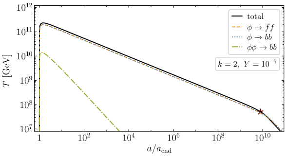
Figure 5: Instantaneous temperature as a function of the scale factor in the supersymmetric scenario (6.3) with a quadratic inflaton potential. Here $m_{{\rm{\it eff}}}\neq 0$ and $\lambda=2.5\times 10^{-11}$, assuming T-attractor inflation boundary conditions. The star signals inflation-radiation equality.

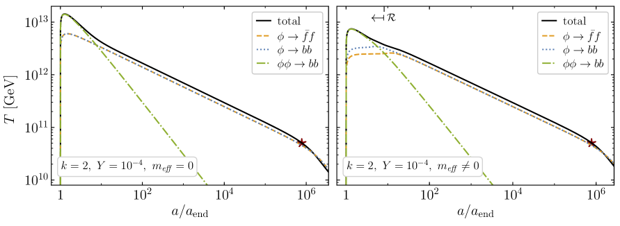
Figure 6: Instantaneous temperature as a function of the scale factor in the supersymmetric scenario (6.3) with a quadratic inflaton potential. Left: $m_{{\rm{\it eff}}}=0$. Right: $m_{{\rm{\it eff}}}\neq 0$. Here $\lambda=2.3\times 10^{-11}$, assuming T-attractor inflation boundary conditions. The star signals inflation-radiation equality. The arrow points toward the region where $\mathcal{R}>1$ for one or more of the decay channels.

Fig. 6 shows the scale factor dependence of the temperature for a larger value of the coupling, $Y=10^{-4}$. The left panel depicts what the evolution of $T$ would be during reheating in the absence of oscillation-induced effective masses. We observe here the equality of fermion and boson decay rates, with a maximum temperature determined in this case by the scattering process, a scenario similar to that shown in Fig. 3. The right panel in turn shows the resulting evolution $T(a)$ including the induced masses of the decay products. Recalling that for all three processes, for $k=2$, the suppression in the width decreases with time, we note that the differences with respect to the left panel are present only for $a\lesssim 20\,a_{\rm end}$. In this regime, the symmetry between the fermionic and bosonic rates is broken due to condensate effects, and $\phi\rightarrow bb^{*}$ dominates over $\phi\rightarrow\bar{f}f$. Nevertheless, despite the noticeable decrease in $T_{\rm max}$, by a factor of $\sim 1.9$, $\phi\phi\rightarrow bb^{*}$ controls the production of relativistic particles at very early times, as it does when $m_{{\rm{\it eff}}}=0$.

For a quartic potential, with $\partial_{\Phi}F=\sqrt{\lambda}\phi^{2}$ near $\phi=0$, only the scattering process occurs at lowest order in the coupling $Y$, with a rate given by

($$k=4 \begin{aligned} \sum_{b}\Gamma_{\phi\phi\rightarrow bb^{*}}\;=\;\frac{Y^{2}\rho_{\phi}}{2.4\pi m_{\phi}^{3}}\Big{\{}&(Y+2\sqrt{\lambda})^{2}\alpha_{\sigma}(\mathcal{R})_{\sigma\rightarrow Y(Y+2\sqrt{\lambda})/2}\\ &+(Y-2\sqrt{\lambda})^{2}\alpha_{\sigma}(\mathcal{R})_{\sigma\rightarrow Y(Y-2\sqrt{\lambda})/2}\Big{\}}\,,\end{aligned}$$) (6.7)

(for details see Appendix A.3). It is worth noting that, for the ‘minus’ states with $Y\lesssim 2\sqrt{\lambda}$, an enhancement of the decay rate appears, instead of a suppression. Nevertheless, this enhancement is always $\lesssim 8\%$, and is tied to the process with the smallest branching ratio when it is maximized, making its contribution to $\Gamma_{\phi}$ negligible. The bosonic enhancement that increases with time is therefore not present in this supersymmetric construction.

Fig. 7 shows the temperature during reheating with $k=4$ for $Y=10^{-7}$. As we saw in Fig. 5 for $k=2$, there is no appreciable enhancement or suppression in this case as well. Indeed, for all decay channels $\mathcal{R}\ll 1$. The inflaton decay rate for both effective bosonic channels is identical in this regime, and is suppressed by a factor of $\sim 5$ with respect to the fermionic one. Therefore, $T\propto a^{-3/4}$. A star, located at $a\simeq 7\times 10^{14}a_{\rm end}$, signals inflaton-radiation equality, that is, the end of reheating. Note the decrease of more than 7 orders of magnitude in $T_{\rm RH}$ compared to the quadratic case.

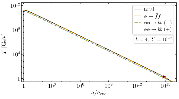
Figure 7: Instantaneous temperature as a function of the scale factor in the supersymmetric scenario (6.3) with a quartic inflaton potential. Here $m_{{\rm{\it eff}}}\neq 0$ and $\lambda=3.3\times 10^{-12}$, assuming T-attractor inflation boundary conditions. The star signals inflation-radiation equality.

The choice of $Y=10^{-4}$ with $k=4$ is displayed in Fig. 8. For this coupling, all decay channels acquire a kinematic suppression. Analogously to the $k=2$ case, the left panel shows the resulting temperature disregarding the inflaton-induced masses for the fermionic and bosonic decay products. Unlike the previous cases though, here it is the scattering of $\phi$ into bosons that most efficiently heats the Universe, to a reheating temperature $T_{\rm RH}\simeq 4\times 10^{8}\,{\rm GeV}$. In the right panel we observe the effect of the kinematic suppression. The fermionic width is reduced by a factor of $7\times 10^{-3}$, while the dominant bosonic widths acquire a suppression $\simeq 2\times 10^{-2}$. This reduction is time-independent, and results in $T_{\rm RH}\simeq 8\times 10^{6}\,{\rm GeV}$.

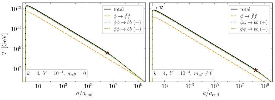
Figure 8: Instantaneous temperature as a function of the scale factor in the supersymmetric scenario (6.3) with a quartic inflaton potential. Left: $m_{{\rm{\it eff}}}=0$. Right: $m_{{\rm{\it eff}}}\neq 0$. Here $\lambda=3.3\times 10^{-12}$, assuming T-attractor inflation boundary conditions. The star signals inflation-radiation equality. The arrow points toward the region where $\mathcal{R}>1$ for one or more of the decay channels.

7 Discussion

7.1 Limitations

Before our summary, we point out a few of the limitations of our analysis. Throughout, we have assumed perturbative reheating processes. Furthermore, we have assumed that the mass of the decay products are genuinely given by the inflaton condensate during the reheating. Thus during an oscillation period, the mass necessarily passes through zero, which may trigger non-perturbative particle production. Whether the non-perturbative production becomes dominant source for $\rho_{R}$ or not depends on the strength of the couplings. For instance, in the case of $\phi\to\bar{f}f$, non-perturbative production becomes non-negligible for $y\gtrsim 10^{-6}$ when $k=2$, and for $y\gtrsim 0.1\sqrt{\lambda}$ when $k=4$ [66]. These values happen to be close to those obtained from ${\cal R}>1$, as can we discuss further in the Appendix. Similar limits for $\phi\to bb$ and $\phi\phi\to bb$ apply and can also be approximated from ${\cal R}>1$ (see, for instance, [67]).

Also, we have not incorporated the thermal corrections to the decay products, which may cause a similar kinetic suppression when the temperature is sufficiently high, compared to the inflaton mass. Although for $k=2$, $m_{\phi}$ is constant, for $k>2$ $m_{\phi}$ decreases slower than the temperature, with $m_{\phi}\propto a^{-1}~{}(k=4)$ and $a^{-3/2}~{}(k=6)$. Therefore, for $\phi\to\bar{f}f$ with $k=4$, we obtain

$$\frac{m_{\rm th}^{2}}{m_{\phi}^{2}}\sim\frac{g^{2}y_{\rm eff}}{2(\lambda^{3}\rho_{\rm end})^{1/8}}\sqrt{\frac{5M_{P}}{6g_{\rho}\pi^{3}}}\left(\frac{a}{a_{\rm end}}\right)^{3/2}\gtrsim 1\quad\ \Rightarrow\quad\ a\gtrsim 1200\,a_{\rm end}\,,$$ (7.1)

for the parameter choices used in Fig. 4, and the adopted thermal mass is $m_{\rm th}\sim gT$ with $g\sim 0.1$. When one considers the cases where thermal masses are greater than the inflaton mass, the thermal dissipation rate of the inflaton should carefully be taken into account, since the inflaton energy density can still be transferred into radiation [68].

For $k\neq 2$, the non-perturbative excitation of non-vanishing momentum modes of the inflaton can also be sourced by the self-interaction of $\phi$. Not only this can have a significant effect on the production rate of daughter particles, but it can also lead to the fragmentation of the inflaton condensate. It has been shown [69, 70] that neglecting inflaton-matter couplings for a potential of the form (2.3), disrupts the condensate occurs through a narrow self-resonance, and leads to its fragmentation after $\mathcal{O}(5)$ $e$-folds for $k=4$. Similar conclusions can be derived in the presence of the four-body interaction $\phi^{2}b^{2}$ [71]. Nevertheless, estimating the duration of the condensate in the presence of generic matter decay channels, and its effect on the dark matter abundance, lies beyond the scope of this work.

7.2 Summary

An essential feature of any inflationary model is its ability to reheat the Universe after a period of exponential expansion. In some cases, it is sufficient to know that the Universe reheat to a certain temperature $T_{\rm RH}$ and that equilibrium was established, and a period of radiation dominated expansion ensued. If the reheat temperature is sufficiently high to allow for baryogenesis, nucleosynthesis, and the production of weakly interacting dark matter the details of the reheating process may not be important. However, for the production of superweakly interacting dark matter, which never attains thermal equilibrium, these details may be essential for determining the relic abundance.

When one goes beyond the instantaneous reheating approximation, one finds that if thermalization is sufficiently rapid, the first few decay products begin to heat the Universe to a temperature, $T_{\rm max}$, which could be much larger than $T_{\rm RH}$ [5, 7], though the energy density in the newly created radiation bath is much less than that stored in the ongoing inflaton oscillations. Typically we expect that during reheating the temperature falls off slowly with the expansion, $T\sim a^{-3/8}$ as more energy is pumped into the thermal bath from continual decays. Dark matter production may be sensitive to the maximum temperature (and the evolution to down to $T_{\rm RH}$) if its production cross section is proportional to $T^{n}$ with $n>6$.

In this paper, we have considered several important aspects of the reheating process. First, the evolution of the temperature, $T(a)$ depends on the form of the inflaton potential controlling the period of inflaton oscillations [16, 9]. For $V(\phi)\propto\phi^{k}$, the evolution is certainly sensitive to $k$ which affects the equation of state during oscillations. However, for $k>2$, the mass of the inflaton and hence its decay rate are also dependent on $k$ and also affects the evolution of the temperature. Second, the evolution depends on the spin statistics of the dominant final state of inflaton decay. We have shown that the temperature evolution differs depending on whether the inflaton decays predominantly to fermions or bosons, or whether annihilations to boson are the main channel depleting the oscillations. For $k=2$, $T\sim a^{-3/8}$ for both fermionic and bosonic final states, and annihilations are incapable of reheating the Universe. However, for $k>2$, the behaviour differs, and annihilations are capable of reheating. Third, while we noted that for $k>2$, the inflaton mass also undergoes a damped oscillation, for all $k$, the masses of the final state particles also depend on the inflaton field value. This may cause the effective final state mass to exceed the inflaton mass and lead to a suppression in the decay rate (for fermionic final states and annihilations) or an enhancement (for bosonic final states). We have used the thermal production of dark matter as an application of these results.

There are several stones left unturned in our analysis. For sufficiently large couplings, non-perturbative effects can not be neglected. Thus parametric resonance may also play a role in the reheating process. We have also set aside the question of direct couplings of the inflaton to dark matter. In this case, the evolution and abundance of dark matter will depend on both the statistics of final state initializing the thermal bath, and the spin of the dark matter particle. The thermal contribution to final state masses may also be important. Finally, it is important to re-examine the validity of the instantaneous thermalization approximation used in this work.

Appendix A The Boltzmann equation for a decaying condensate

In this appendix we derive the evolution equation for the energy density of the inflaton condensate from the particle perspective. Under the assumption that the decay of the inflaton is perturbative, then the condensate, $\phi$, is spatially homogeneous, and its phase space distribution may be written as $f_{\phi}(k,t)=(2\pi)^{3}n_{\phi}(t)\delta^{(3)}(\bm{k})$, with $n_{\phi}$ the instantaneous inflaton number density. Disregarding Bose enhancement / Pauli blocking effects for the $\phi$-decay products, the integrated Boltzmann equation for the number density can be written as follows [72],

$$\dot{n}_{\phi}+3Hn_{\phi}\;=\;-\int d\Psi_{\phi,A,B}\,|\mathcal{M}|^{2}_{\phi\rightarrow AB}f_{\phi}(k,t)\,,$$ (A.1)

where $A,B$ denote the decay products of $\phi$, $d\Psi_{\phi,A,B}$ is the phase space measure for the particles $A,B$ and the condensate $\phi$, and $\mathcal{M}$ denotes the transition amplitude. More precisely,

$$d\Psi_{\phi,A,B}\,|\mathcal{M}|^{2}_{\phi\rightarrow AB}\;=\;\sum_{n=1}^{\infty}\frac{d^{3}\bm{k}}{(2\pi)^{3}n_{\phi}(t)}\frac{d^{3}\bm{p}_{A}}{(2\pi)^{3}2p_{A}^{0}}\frac{d^{3}\bm{p}_{B}}{(2\pi)^{3}2p_{B}^{0}}(2\pi)^{4}\delta^{(4)}(p_{n}-p_{A}-p_{B})|\mathcal{M}_{n}|^{2}\,,$$ (A.2)

where now $\mathcal{M}_{n}$ denote the transition amplitude in one oscillation for each oscillating field mode of $\phi$ from the coherent state $|\phi\rangle$ to the two-particle final state $|A,B\rangle$. Below we perform a few explicit computations for it. Note here that the seemingly Lorentz non-invariant factor of $1/n_{\phi}$ is needed so that the inflaton measure is correctly normalized by

$$\int\frac{d^{3}\bm{k}}{(2\pi)^{3}n_{\phi}}\,f_{\phi}(k,t)\;=\;1\,.$$ (A.3)

Integration with respect to the $\phi$ momentum gives

$$\dot{n}_{\phi}+3Hn_{\phi}\;=\;-\sum_{n=1}^{\infty}\int\frac{d^{3}\bm{p}_{A}}{(2\pi)^{3}2p_{A}^{0}}\frac{d^{3}\bm{p}_{B}}{(2\pi)^{3}2p_{B}^{0}}(2\pi)^{4}\delta^{(4)}(p_{n}-p_{A}-p_{B})|\mathcal{M}_{n}|^{2}\,,$$ (A.4)

where now $p_{n}=(E_{n},\bm{0})$, $E_{n}$ denoting the energy of the $n$-th oscillation mode of $\phi$. Note that the matrix element in Eq. (A.4) effectively contains the condensate, thereby absorbing the factor of $n_{\phi}$ that would be expected to be present on the right-hand side of (A.4).

The evolution equation for the energy density of $\phi$ can be obtained by noting that, on the right-hand side, we must introduce the energy of each oscillation mode $|\mathcal{M}_{n}|^{2}\rightarrow|\mathcal{M}_{n}|^{2}E_{n}$. On the left side of the equality, the adiabaticity assumption for the decay (cf. (2.10)) implies that only the lowest oscillation mode must be taken into account, so that $\rho_{\phi}=m_{\phi}n_{\phi}$, where $m_{\phi}$ has been defined in (3.3). Developing the time derivative we find

$$\dot{\rho}_{\phi}\;=\;-3H\left(-\frac{\partial_{t}m_{\phi}^{2}}{6Hm_{\phi}^{2}}\right)\rho_{\phi}+m_{\phi}\dot{n}_{\phi}\,.$$ (A.5)

To simplify the first term on the right-hand side of the equality, we note that, from Eqs. (2.10) and (2.12), it is straightforward to verify that the equation of motion for $\phi_{0}$ on short time-scales is given by

$$\dot{\phi}_{0}\;\simeq\;-\frac{6}{k+2}H\phi_{0}\,.$$ (A.6)

From the definition of the effective mass, Eq. (3.3), we then have

$$-\frac{\partial_{t}m_{\phi}^{2}}{6Hm_{\phi}^{2}}\;=\;\frac{(2-k)\dot{\phi}_{0}}{6H\phi_{0}}\;=\;\frac{k-2}{k+2}\,.$$ (A.7)

Therefore, upon comparison with (2.13), and substitution of (A.4), we obtain

$$\dot{\rho}_{\phi}+3H(1+w_{\phi})\rho_{\phi}\;=\;-(1+w_{\phi})\Gamma_{\phi}\rho_{\phi}\,,$$ (A.8)

where the right-hand side is given by the energy transfer per space-time volume (Vol₄), defined as

$$(1+w_{\phi})\Gamma_{\phi}\rho_{\phi}\equiv\frac{\Delta E}{{\rm Vol}_{4}},$$ (A.9)

$$\Delta E\equiv\int\frac{d^{3}\bm{p}_{A}}{(2\pi)^{3}2p_{A}^{0}}\frac{d^{3}\bm{p}_{B}}{(2\pi)^{3}2p_{B}^{0}}(p_{A}^{0}+p_{B}^{0})|\langle{\rm f}|i\int d^{4}x{\cal L}_{I}|0\rangle|^{2}$$ (A.10)

with ${\cal L}_{I}$ being the interaction Lagrangian. Substituting

$$|\langle{\rm f}|i\int d^{4}x{\cal L}_{I}|0\rangle|^{2}={\rm Vol}_{4}\sum_{n=-\infty}^{\infty}|{\cal M}_{n}|^{2}(2\pi)^{4}\delta^{4}(p_{n}-p_{A}-p_{B}),$$ (A.11)

to Eq. (A.10), we obtain [59, 55]

$$\Gamma_{\phi}=\frac{1}{8\pi(1+w_{\phi})\rho_{\phi}}\sum_{n=1}^{\infty}|{\cal M}_{n}|^{2}E_{n}\beta_{n}(m_{A},m_{B}),$$ (A.12)

$$\beta_{n}(m_{A},m_{B})\equiv\sqrt{\left(1-\frac{(m_{A}+m_{B})^{2}}{E_{n}^{2}}\right)\left(1-\frac{(m_{A}-m_{B})^{2}}{E_{n}^{2}}\right)}.$$ (A.13)

We may write $E_{n}=n\omega$, with $\omega$ being the frequency of oscillation of $\phi$, which decreases with the envelope $\phi_{0}$ for $k>2$. With $\phi(t)\simeq\phi_{0}(t)\cdot\mathcal{P}(t)$, approximating $\phi_{0}$ as constant over one oscillation we obtain

$$\dot{\mathcal{P}}^{2}\;=\;\frac{2\rho_{\phi}}{\phi_{0}^{2}}\left(1-\mathcal{P}^{k}\right)\;=\;\frac{2m_{\phi}^{2}}{k(k-1)}\left(1-\mathcal{P}^{k}\right)\,.$$ (A.14)

Straightforward integration gives

$$\omega\;=\;m_{\phi}\sqrt{\frac{\pi k}{2(k-1)}}\,\frac{\Gamma(\frac{1}{2}+\frac{1}{k})}{\Gamma(\frac{1}{k})}\,.$$ (A.15)

In term of this frequency we can write

$$\mathcal{P}(t)\;=\;\sum_{n=-\infty}^{\infty}\mathcal{P}_{n}e^{-in\omega t}.$$ (A.16)

A.1 Inflaton decay to a pair of fermions

Let us evaluate explicitly the decay rate for the energy density of $\phi$ when it decays to a pair of fermions. Assume now an inflaton-matter coupling of the form $\mathcal{L}_{I}=y\phi\bar{f}f$. In the amplitude ${\cal M}_{n}$ we replace $\phi$ with $\phi_{0}{\cal P}_{n}$ (as it is treated as an interaction coefficient) and obtain

$${\cal M}_{n}=y\phi_{0}{\cal P}_{n}\bar{u}(p_{A})v(p_{B}),$$ (A.17)

and thus, averaging over oscillations,

$$\Gamma_{\phi\rightarrow\bar{f}f}\; =\;\frac{y^{2}\phi_{0}^{2}\omega^{3}}{4\pi(1+w_{\phi})\rho_{\phi}}\sum_{n=1}^{\infty}n^{3}|\mathcal{P}_{n}|^{2}\left\langle\beta_{n}^{3}(m_{f},m_{f})_{+}\right\rangle$$

$$=\;\frac{y^{2}}{8\pi}\omega\left[(k+2)(k-1)\left(\frac{\omega}{m_{\phi}}\right)^{2}\sum_{n=1}^{\infty}n^{3}|\mathcal{P}_{n}|^{2}\left\langle\left(1-\left(\frac{2m_{f}}{n\omega}\right)^{2}\right)^{3/2}_{+}\right\rangle\right]$$

$$=\;\frac{y^{2}}{8\pi}\omega\left[(k+2)(k-1)\left(\frac{\omega}{m_{\phi}}\right)^{2}\sum_{n=1}^{\infty}n^{3}|\mathcal{P}_{n}|^{2}\left\langle\left(1-\frac{\mathcal{R}}{n^{2}}\mathcal{P}^{2}\right)^{3/2}_{+}\right\rangle\right]$$

$$\equiv\;\frac{y^{2}}{8\pi}\omega\,\alpha_{y}(k,\mathcal{R})\,.$$ (A.18)

Note here that $\mathcal{R}=(2m_{f}/\omega)^{2}|_{\phi\rightarrow\phi_{0}}$ (see Eq. (3.7)). Here we have introduced the notation

$$(1-x)_{+}\;\equiv\;(1-x)\,\theta(1-x)\,,$$ (A.19)

where $\theta$ is the Heaviside step function. This ensures that the decay only occurs when it is (instantaneously) kinematically allowed. Comparing (A.18) and (3.2), we finally identify

$$y_{{\rm{\it eff}}}^{2}(k)\;=\;\alpha_{y}(k,\mathcal{R})\frac{\omega}{m_{\phi}}y^{2}\,.$$ (A.20)

Fig. 9 shows the $k$-dependence of the function $\alpha_{y}(k,0)$, that is, in the massless fermion limit. Realistically though, $m_{f}\neq 0$ even if in the vacuum $m_{f}=0$. The dependence on the effective mass of $f$, induced by the oscillating background, is quantified through $\mathcal{R}$ and shown in Fig. 10 for $k=2,4,6$. For $\mathcal{R}\ll 1$, the rate at $m_{f}=0$ can be used. For $\mathcal{R}\gtrsim\mathcal{O}(10^{-1})$ the inflaton-induced mass for $f$ becomes comparable to $m_{\phi}$, and for $\mathcal{R}\gg 1$ the effective decay rate is suppressed as $\alpha_{y}(k,\mathcal{R})\propto\mathcal{R}^{-1/2}\alpha_{y}(k,0)$ (or $\Gamma_{\phi\rightarrow\bar{f}f}\propto\mathcal{R}^{-1/2}$). The constant of proportionality is approximately $0.38$ for $k=2$, $0.50$ for $k=4$ and $0.61$ for $k=6$. It is worth noting that, although the kinematic suppression is less severe for higher harmonics in (A.18), this relative enhancement of the rate is over-compensated by the exponential suppression of the $\mathcal{P}_{n}$. In fact, approximating the kinematic blocking by means of the first harmonic only, a maximum error of $\sim 20\%$ is made (for $k=6$ and $\mathcal{R}\gg 1$).

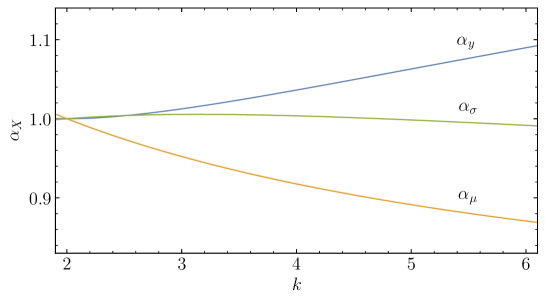
Figure 9: Numerical value of the sub-leading corrections to the effective inflaton matter-couplings $y$, $\mu$ and $\sigma$. These functions are computed as sums of coefficients of the Fourier expansion of powers of the exact solution of the equation of motion for $\phi$. Here $m_{{\rm{\it eff}}}=0$.

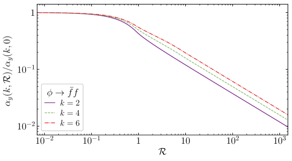
Figure 10: Kinematic factor for the oscillation-average of the decay rate $\Gamma_{\phi\rightarrow\bar{f}f}$.

A.2 Inflaton decay to a pair of bosons

Let us now consider an inflaton-matter coupling of the form $\mathcal{L}_{I}=\zeta^{2-\gamma}\phi^{\gamma}b_{1}b_{2}$, where $\gamma$ is an arbitrary integer exponent. Again, we may replace $\phi^{\gamma}$ with $\phi_{0}^{\gamma}({\cal P^{\gamma}})_{n}$ in ${\cal M}_{n}$, where the expression $\left(\mathcal{P}^{\gamma}\right)_{n}$ denote the Fourier coefficients of the expansion of $\mathcal{P}^{\gamma}(t)$, and obtain $\mathcal{M}_{n}=\zeta^{2-\gamma}\phi_{0}^{\gamma}\left(\mathcal{P}^{\gamma}\right)_{n}$. Substitution of the squared amplitude in (A.12) immediately gives

$$\Gamma_{\phi^{\gamma}\rightarrow b_{1}b_{2}}\;=\;\frac{\zeta^{4-2\gamma}\phi_{0}^{2\gamma}}{8\pi(1+w_{\phi})\rho_{\phi}}\omega\sum_{n=1}^{\infty}n|\left(\mathcal{P}^{\gamma}\right)_{n}|^{2}\left\langle\beta_{n}(m_{1},m_{2})_{+}\right\rangle\,.$$ (A.21)

For the case $\phi\rightarrow bb$, with $\gamma=1$ and $\zeta=\mu$, and including the appropriate symmetry factors, we obtain (3.4), with

$$\mu_{{\rm{\it eff}}}^{2}(k)\; =\;\frac{1}{4}(k+2)(k-1)\frac{\omega}{m_{\phi}}\left[4\sum_{n=1}^{\infty}n|\mathcal{P}_{n}|^{2}\left\langle\left(1-\frac{\mathcal{R}}{n^{2}}\mathcal{P}\right)^{1/2}_{+}\right\rangle\right]\mu^{2}$$

$$\equiv\;\frac{1}{4}(k+2)(k-1)\frac{\omega}{m_{\phi}}\alpha_{\mu}(k,\mathcal{R})\mu^{2}\,.$$ (A.22)

Here $\mathcal{R}=(2m_{b}/\omega)^{2}|_{\phi\rightarrow\phi_{0}}$ is also given by the middle line of (3.7). The numerically computed function $\alpha_{\mu}$ in the limit $m_{b}\ll m_{\phi}$ is shown in Fig. 9. One can account for the inflaton-induced effective mass of $b$, assuming for simplicity a vanishing bare mass. The result of the numerical calculation of the average over one oscillation is shown in Fig. 11. Notably, in this case, the approximation which uses the first harmonic accounts for $\gtrsim 99\%$ of the kinematic effect. As expected, for low values of the inflaton-matter coupling, $\mathcal{R}\ll 1$, the induced mass $m_{{\rm{\it eff}}}$ can be safely neglected. However, as $\mathcal{R}\gtrsim 1$, the value of $\alpha_{\mu}(k,\mathcal{R})$ deviates from that of $\alpha_{\mu}(k,0)$, and in fact appears to grow as $\mathcal{R}^{1/2}$ for $\mathcal{R}\gtrsim 5$. Numerically, this occurs due to the linear dependence on $\phi$ of the effective mass of $b$ (c.f. Eq. (3.6)), meaning that for sufficiently large $\mathcal{R}$ the argument of the square root in (A.22) will be positive for half of the oscillation. Physically, this signals the breakdown of perturbativity and the need to account for (tachyonic) preheating effects.

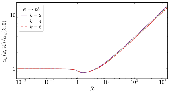
Figure 11: Kinematic factor for the oscillation-average of the decay rate $\Gamma_{\phi\rightarrow bb}$.

In the “scattering” scenario $\phi\phi\rightarrow bb$, using ${\cal L}_{I}=\sigma\phi^{2}b^{2}$, we obtain ${\cal M}_{n}=2\sigma\phi_{0}^{2}({\cal P}^{2})_{n}$, and thus

$$\Gamma_{\phi\phi\to bb}=\frac{\sigma^{2}\phi_{0}^{4}}{4\pi(1+w_{\phi})\rho_{\phi}}\omega\sum_{n=1}^{\infty}n|({\cal P}^{2})_{n}|^{2}\left\langle\beta_{n}(m_{b},m_{b})_{+}\right\rangle.$$ (A.23)

For $k=2$, using $\sum_{n=1}^{\infty}n|({\cal P}^{2})_{n}|^{2}=1/8$ and $\phi_{0}^{4}=(2\rho_{\phi}/m_{\phi}^{2})^{2}$, we recover $\Gamma_{\phi\phi\to bb}=\sigma^{2}\rho_{\phi}/8\pi m_{\phi}^{3}$ when $m_{b}=0$. We analogously obtain that

$$\sigma^{2}_{{\rm{\it eff}}}(k)\; =\;\frac{1}{8}k(k+2)(k-1)^{2}\frac{\omega}{m_{\phi}}\left[8\sum_{n=1}^{\infty}n|\left(\mathcal{P}^{2}\right)_{n}|^{2}\left\langle\left(1-\frac{\mathcal{R}}{n^{2}}\mathcal{P}^{2}\right)^{1/2}_{+}\right\rangle\right]\sigma^{2}$$

$$\equiv\;\frac{1}{8}k(k+2)(k-1)^{2}\frac{\omega}{m_{\phi}}\alpha_{\sigma}(k,\mathcal{R})\sigma^{2}\,,$$ (A.24)

where the numerically calculated $\alpha_{\sigma}(k,0)$ is shown in Fig. 9. Here $\mathcal{R}=(2m_{b}/\omega)^{2}|_{\phi\rightarrow\phi_{0}}$, also given in Eq. (3.7). Similarly to the fermionic decay case, the presence of the kinematic factor will result in a suppression of the effective decay rate of $\phi$ at large $\mathcal{R}$. Fig. 12 shows this effect for $k=2,4,6$. For $\mathcal{R}\ll 1$, the limit $m_{b}=0$ is appropriate. For $\mathcal{R}\gg 1$, $\alpha_{\sigma}(k,\mathcal{R})\propto\mathcal{R}^{-1/2}\alpha_{\sigma}(k,0)$, with constant of proportionality equal to $1.00$, $1.22$ and $1.35$ for $k=2,4$ and $6$, respectively.

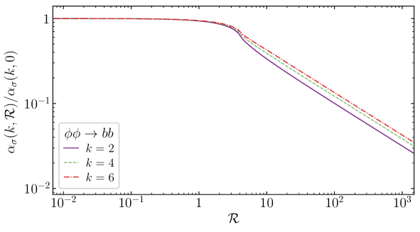
Figure 12: Kinematic factor for the oscillation-average of the decay rate $\Gamma_{\phi\phi\rightarrow bb}$.

A.3 Supersymmetric kinematic factors

The computation of the decay rates for the supersymmetric scenario discussed in Section 6 follows immediately from the previous discussion. The main difference corresponds to the two terms that source the effective mass of bosons, proportional to $Y^{2}\phi^{2}$ and $Y\partial_{\Phi}F(\phi)$, as shown in Eq. (6.4). For $k=2$, $\partial_{\Phi}F(\phi)=m_{\phi}\phi/\sqrt{2}$. In this case it is convenient to write

$$\mathcal{R}\;=\;\frac{Y^{2}\phi_{0}^{2}}{2m_{\phi}^{2}}\,,$$ (A.25)

so that the corresponding oscillation-averaged phase-space factor, which we denote simply by the corresponding channel, is given by

$$\alpha_{\phi\rightarrow bb^{*}}(\mathcal{R})\; =\;\left\langle\left(1-4\mathcal{R}\mathcal{P}^{2}\mp 4\sqrt{\mathcal{R}}\mathcal{P}\right)^{1/2}_{+}\right\rangle\,,$$ (A.26)

$$\alpha_{\phi\phi\rightarrow bb^{*}}(\mathcal{R})\; =\;\left\langle\left(1-\mathcal{R}\mathcal{P}^{2}\mp\sqrt{\mathcal{R}}\mathcal{P}\right)^{1/2}_{+}\right\rangle\,,$$ (A.27)

(only the first harmonic contributes). Fig. 13 shows the magnitude of this suppression factor, as the continuous blue curve for the decay process, and the dashed yellow curve for the scattering channel.

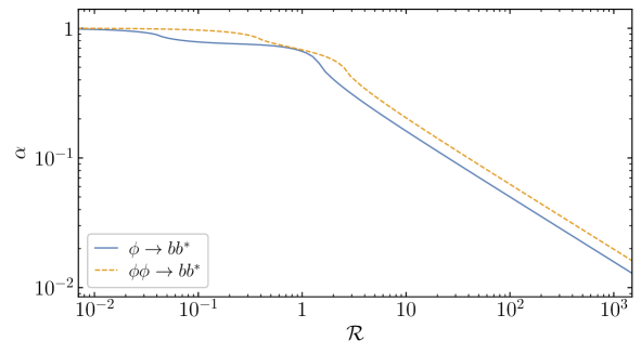
Figure 13: Kinematic factor for the oscillation-averaged decay rates (6.6) for the supersymmetric model (6.3).

For $k=4$, $\partial_{\Phi}F(\phi)=\sqrt{\lambda}\phi^{2}$. Therefore, only the scattering process for bosons is present at lowest order. In this scenario, with the identification $\sigma\rightarrow Y(Y\pm 2\sqrt{\lambda})/2$ in (3.7), we write

$$\mathcal{R}_{\pm}\;\simeq\;1.4\frac{Y}{\lambda}\left(Y\pm 2\sqrt{\lambda}\right)\,.$$ (A.28)

and

$$\alpha_{b,\pm}\;=\;8\sum_{n=1}^{\infty}n|\left(\mathcal{P}^{2}\right)_{n}|^{2}\left\langle\left(1-\frac{\mathcal{R_{\pm}}}{n^{2}}\mathcal{P}^{2}\right)^{1/2}_{+}\right\rangle\,.$$ (A.29)

Note that, unlike previous cases, here $\mathcal{R}_{\pm}$ can be positive or negative, depending on the magnitude of $Y$ relative to $2\sqrt{\lambda}$. For the T-attractor, $\sqrt{\lambda}\simeq 1.8\times 10^{-6}$. In Fig. 14 the result of the numerical evaluation of (A.29) for the T-attractor is presented, as a function of $Y$. We note that, for $\alpha_{b,+}$, only a suppression in the rate is observed. Shown also in the figure are the values for $\alpha_{\sigma}(\mathcal{R}_{+})$, which are identical to those for $\alpha_{b,+}$. On the other hand, for $\alpha_{b,-}$ an enhancement $<\mathcal{O}(1)$ in the rate is observed for $Y<2\sqrt{\lambda}$, which corresponds to the range in which $\mathcal{R}_{-}$ is negative. For larger values of the coupling, the decay rate of $\phi$ is suppressed. In Fig. 14 the oscillation average of $\alpha_{\sigma}(\mathcal{R}_{-})$ is also shown, assuming it is equal to 1 for negative $\mathcal{R}_{-}$. This quantity matches the behavior of $\alpha_{b,-}$.

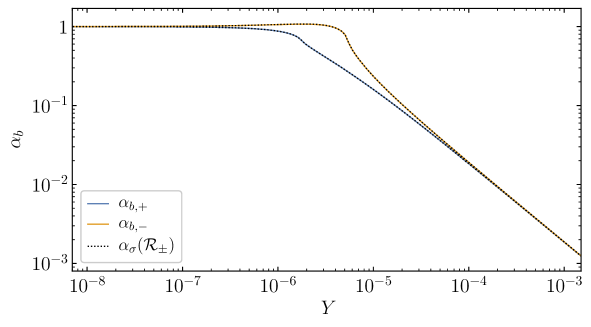
Figure 14: Kinematic factor for the oscillation-averaged decay rates (6.7) for the supersymmetric model (6.3) with $k=4$. Here the T-attractor value $\lambda\simeq 3.3\times 10^{-12}$ has been chosen for definiteness.

Appendix B T-attractor inflation

The rates at which energy densities and temperatures change during reheating depend not only on the shape of the potential (2.4), parametrized by $k$, but also on its normalization, parametrized by $\lambda$, which in turn is determined by the amplitude of the power spectrum of curvature fluctuations. Moreover, the initial condition for $\rho_{\phi}$ depends on the value of the scalar field $\phi$ at the end of inflation. In this Appendix we determine the boundary conditions for $\lambda$ and $\rho_{\rm end}$ under the assumption that the scalar potential responsible for inflation is of the T-model form (2.3).

Inflation is defined as a period of accelerated expansion. Its end is therefore defined as the condition $\ddot{a}=0$, which can be shown to be equivalent to $\dot{\phi}_{\rm end}^{2}=V(\phi)$ [73]. An approximate solution for these conditions for arbitrary $k$ is given by

$$\phi_{\rm end}\;=\;\sqrt{\frac{3}{8}}\,M_{P}\ln\left[\frac{1}{2}+\frac{k}{3}\left(k+\sqrt{k^{2}+3}\right)\right]\,.$$ (B.1)

The energy density is in turn determined as $\rho_{\rm end}=\frac{3}{2}V(\phi_{\rm end})$. The normalization of the potential can be determined from the inflationary slow role parameters as follows. Given the potential in Eq. (2.3), the slow roll parameters, $\epsilon$ and $\eta$ are

$$\epsilon\;\equiv\;\frac{1}{2}M_{P}^{2}\left(\frac{V^{\prime}}{V}\right)^{2}\;=\;\frac{k^{2}}{3}{\rm csch}^{2}\left(\sqrt{\frac{2}{3}}\frac{\phi}{M_{P}}\right)\,,$$ (B.2)

and

$$\eta\;\equiv\;M_{P}^{2}\left(\frac{V^{\prime\prime}}{V}\right)\;=\;\frac{2}{3}k\left[k-\cosh\left(\sqrt{\frac{2}{3}}\frac{\phi}{M_{P}}\right)\right]{\rm csch}^{2}\left(\sqrt{\frac{2}{3}}\frac{\phi}{M_{P}}\right)\,.$$ (B.3)

The number of $e$-folds between the exit of the horizon of the scale $k_{*}$ at $\phi_{*}$, and the end of inflation at $\phi_{\rm end}$, can be computed in the slow-roll approximation as follows,

$$N_{*}\;\simeq\;\frac{1}{M_{P}^{2}}\int_{\phi_{\rm end}}^{\phi_{*}}\frac{V(\phi)}{V^{\prime}(\phi)}\,d\phi\;\simeq\;\int^{\phi_{*}}_{\phi_{\rm{end}}}\frac{1}{\sqrt{2\epsilon}}\frac{d\phi}{M_{P}}\;\simeq\;\frac{3}{2k}\cosh\left(\sqrt{\frac{2}{3}}\frac{\phi_{*}}{M_{P}}\right)\,.$$ (B.4)

In the slow-roll approximation, the scalar tilt $n_{s}$ and the tensor-to-scalar ratio $r$ are given by the following expressions,

$$n_{s}\; \simeq\;1-6\epsilon_{*}+2\eta_{*}\;=\;1-\frac{2k^{2}(4N_{*}+3)}{4k^{2}N_{*}^{2}-9}\;\simeq\;1-\frac{2}{N_{*}}-\frac{3}{2N_{*}^{2}}\,,$$ (B.5)

$$r\; \simeq\;16\epsilon_{*}\;=\;\frac{48k^{2}}{4k^{2}N_{*}^{2}-9}\;\simeq\;\frac{12}{N_{*}^{2}}\,.$$ (B.6)

Finally, the amplitude of the curvature power spectrum can be expressed as

$$A_{S*}\;\simeq\;\frac{V_{*}}{24\pi^{2}\epsilon_{*}M_{P}^{4}}\;\simeq\;\frac{6^{\frac{k}{2}}}{8k^{2}\pi^{2}}\lambda\sinh^{2}\left(\sqrt{\frac{2}{3}}\frac{\phi_{*}}{M_{P}}\right)\tanh^{k}\left(\frac{\phi_{*}}{\sqrt{6}M_{P}}\right)\,,$$ (B.7)

where $V_{*}=V(\phi_{*})$. For the Planck pivot scale $k_{*}=0.05\,{\rm Mpc}^{-1}$, $\ln(10^{10}A_{S*})=3.044$ [74, 2]. Thus to determine the normalization of the potential given by $\lambda$, we must first obtain $\phi_{*}$ through $N_{*}$. A good approximation is given by

$$\lambda\;\simeq\;\frac{18\pi^{2}A_{S*}}{6^{k/2}N_{*}^{2}}\,.$$ (B.8)

which can be obtained by substitution of $\phi_{*}(N_{*})$ in the expression for $A_{S*}$ and is good to 3% for $N_{*}\in(50,60)$.

The number of $e$-folds, $N_{*}$, can be computed in a self-consistent way assuming there is no entropy production between the end of reheating and the reentry to the horizon of the scale $k_{*}$ in the radiation or matter-dominated eras. The value of $N_{*}$ depends on the energy scale of inflation and the duration of reheating, as measured by the deviation of the total equation-of-state parameter $w$ from its value during radiation domination, $w=1/3$. More precisely, [57, 75],

$$N_{*}\;=\;\ln \left[\frac{1}{\sqrt{3}}\left(\frac{\pi^{2}}{30}\right)^{1/4}\left(\frac{43}{11}\right)^{1/3}\frac{T_{0}}{H_{0}}\right]-\ln\left(\frac{k_{*}}{a_{0}H_{0}}\right)+\frac{1}{4}\ln\left(\frac{V_{*}^{2}}{M_{P}^{4}\rho_{\rm end}}\right)$$

$$+\frac{1-3w_{\rm int}}{12(1+w_{\rm int})}\ln\left(\frac{\rho_{\rm rad}}{\rho_{\rm end}}\right)-\frac{1}{12}\ln g_{\rm reh}\,.$$ (B.9)

The present photon temperature and Hubble parameter, as determined from CMB observations, are given by $T_{0}=2.7255\,{\rm K}$ and $H_{0}=67.36\,{\rm km}\,{\rm s}^{-1}\,{\rm Mpc}^{-1}$, respectively [74, 76]. The scale factor at the present time is normalized as $a_{0}=1$. The energy at the beginning of the $w=1/3$ era is denoted by $\rho_{\rm rad}$. Note that in general $\rho_{\rm reh}\geq\rho_{\rm rad}$, as $1/3\geq w\geq w_{\phi}$ at inflaton-radiation equality. Finally, $w_{\rm int}$ denotes the $e$-fold average of the equation-of-state parameter during reheating,

$$w_{\rm int}\;\equiv\;\frac{1}{N_{\rm rad}-N_{\rm end}}\int_{N_{\rm end}}^{N_{\rm rad}}w(n)\,dn\,.$$ (B.10)

The solution of (B.9) for $N_{*}$ must be found numerically in general. We solve it by iteration. Namely, using Eq. (B.8) to determine $\lambda$ and $V_{*}$ in (B.9) allows for a simple solution for $N_{*}$ if one approximates $w_{\rm int}\approx w_{\phi}$ and $\rho_{\rm rad}\approx\rho_{\rm reh}$, the later given by $T_{\rm RH}$. One can then substitute into (B.7) and use it as a boundary condition for the numerical solution of the system (2.12)-(2.15), which permits a better determination of $w_{\rm int}$ and $\rho_{\rm rad}$, and hence of $N_{*}$. This method converges rapidly, to the second decimal place after only one iteration.

A few features are common to all inflaton depletion processes. For $k=4$, $w_{\phi}=1/3$, and the number of $e$-folds is independent on the details of reheating and is always equal to 55.9 for T-attractor inflation. Note also that for any value of $k$ the CMB parameters $n_{s}$ and $r$ converge to the same attractor limit at $N_{*}\gg 1$. This feature allows the identification of a domain of $e$-folds compatible with Planck data combined with BICEP2/Keck results [74, 2]. At 68%, $45.2\lesssim N_{*}\lesssim 76.7$, while at 95%, $49.7\lesssim N_{*}\lesssim 66.7$.

Fig. 15 shows the numerical solution for $N_{*}$ for the perturbative decay of the inflaton into fermions for $k=2,4$. The whole parameter space depicted there lies within the Planck+BICEP2/Keck 95% CL region for the scalar tilt $n_{s}$ at low tensor-to-scalar ratio. The 68% CL exclusion region is shown in light red. The excluded region in gray corresponds to reheating temperatures lower than $1\,{\rm MeV}$, incompatible with big bang nucleosynthesis [62, 63]. The region in light orange corresponds to values of the Yukawa coupling for which a kinematic suppression is present until some time $t_{\mathcal{R}}\geq t_{\rm max}$ (c.f. Eq. (4.25)). In the orange region, this kinematic suppression is present until the end of reheating, and therefore the approximation $m_{{\rm{\it eff}}}=0$ leads to an inadequate estimate for the temperature of the inflaton decay products throughout the duration of reheating. We note that, for $k=4$, $w_{\phi}=1/3$, and therefore the number of $e$-folds is $N_{*}\simeq 55.9$, independently of the decay rate. We do not show the values of $N_{*}$ for $k=6$, as in that case the kinematic suppression leads to $T_{\rm RH}<1\,{\rm MeV}$ for $y\lesssim 5\times 10^{-2}$. At larger values of the coupling we expect our approximations to break down.

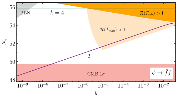
Figure 15: Number of $e$-folds from the exit of the Planck pivot scale to the end of inflation, as a function of $k$ and $y$, for the decay of $\phi$ into fermions. Here the Standard Model value $g_{\rm reh}=427/4$ is used. The gray region is incompatible with Big Bang Nucleosynthesis. The light red region is disfavored at 68% by Planck+BKP.

Fig. 16 shows the numerically calculated number of $e$-folds for the Planck pivot scale for the process $\phi\rightarrow bb$, for $k=2,4,6$. In this case, the light red shaded region is excluded by CMB observations to 68% CL, while the red region is excluded at 95%. In the light orange area, a kinematic enhancement of the decay rate is present from $t_{\rm end}$ to $t_{\mathcal{R}}\geq t_{\rm max}$. In the orange region, the enhancement is present until the end of reheating. For $k=6$ this reduces the value of $N_{*}$, albeit only at the $\mathcal{O}(1\%)$ level. For $k=4$, $N_{*}\simeq 55.9$.

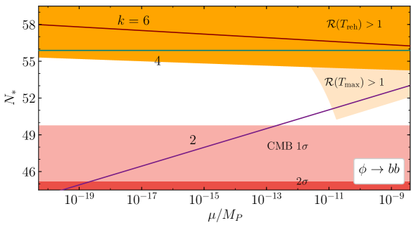
Figure 16: Number of $e$-folds from the exit of the Planck pivot scale to the end of inflation, as a function of $k$ and $\mu$, for the decay of $\phi$ into bosons. Here the Standard Model value $g_{\rm reh}=427/4$ is used. The light red (red) region is disfavored at 68% (95%) by Planck+BKP.

Finally the numerical results for the scattering process $\phi\phi\rightarrow bb$ are shown in Fig. 17. Recall however, that by itself, this process cannot reheat the universe unless $k>3$ (see Table 1). For both $k=4$ and $k=6$, for couplings, $\sigma>10^{-12}$, we are always in a regime where ${\cal R}(T_{\rm RH})>1$.

Figure 17: Number of $e$-folds from the exit of the Planck pivot scale to the end of inflation, as a function of $k$ and $\sigma$, for the scattering of $\phi$ into bosons. Here the Standard Model value $g_{\rm reh}=427/4$ is used.

These results can be used to fix the potential normalization, $\lambda$ and $\rho_{\rm end}$. As one can see from Figs. 15 and 16, the numerically determined value of $N_{*}$ depends on the couplings $y$ and $\mu$ for $k=2$. For $\mu\lower 3.01385pt\hbox{$\;\stackrel{{\scriptstyle\textstyle<}}{{\sim}}\;$}m_{\phi}y$, decays are dominated by fermionic final states and for $k=2$,

$$\lambda\;\simeq\;2.5\times 10^{-11}\left(\frac{10^{-7}}{y}\right)^{1/80}\,,\qquad\rho_{\rm end}\;\simeq\;\left(5.2\times 10^{15}{\rm GeV}\right)^{4}\left(\frac{10^{-7}}{y}\right)^{1/80}\,.$$ (B.11)

When $\mu>m_{\phi}y$, one can place $y$ with $\mu/m_{\phi}$ in (B.11) to obtain $\lambda$ and $\rho_{\rm end}$. For $k=4$, $N_{*}$ does not depend on the choice of couplings, and we have simply

$$\lambda\;\simeq\;3.3\times 10^{-12}\,,\qquad\rho_{\rm end}\;\simeq\;\left(4.8\times 10^{15}{\rm GeV}\right)^{4}\,.$$ (B.12)

References

- [1] K. A. Olive, Phys. Rept. 190 (1990) 307; A. D. Linde, Particle Physics and Inflationary Cosmology (Harwood, Chur, Switzerland, 1990); D. H. Lyth and A. Riotto, Phys. Rep. 314 (1999) 1 [arXiv:hep-ph/9807278]; A. D. Linde, Phys. Rept. 333, 575-591 (2000); J. Martin, C. Ringeval and V. Vennin, Phys. Dark Univ. 5-6, 75-235 (2014) [arXiv:1303.3787 [astro-ph.CO]]; J. Martin, C. Ringeval, R. Trotta and V. Vennin, JCAP 1403 (2014) 039 [arXiv:1312.3529 [astro-ph.CO]]; J. Martin, Astrophys. Space Sci. Proc. 45, 41 (2016) [arXiv:1502.05733 [astro-ph.CO]].
- [2] Y. Akrami et al. [Planck], Astron. Astrophys. 641, A10 (2020) [arXiv:1807.06211 [astro-ph.CO]].
- [3] A. Dolgov and A. D. Linde, Phys. Lett. B 116, 329 (1982); L. Abbott, E. Farhi and M. B. Wise, Phys. Lett. B 117, 29 (1982).
- [4] D. V. Nanopoulos, K. A. Olive and M. Srednicki, Phys. Lett. B 127, 30-34 (1983);
- [5] G. F. Giudice, E. W. Kolb and A. Riotto, Phys. Rev. D 64 (2001) 023508 [hep-ph/0005123]; D. J. H. Chung, E. W. Kolb and A. Riotto, Phys. Rev. D 60 (1999) 063504 [hep-ph/9809453].
- [6] E. Dudas, Y. Mambrini and K. Olive, Phys. Rev. Lett. 119 (2017) no.5, 051801 [arXiv:1704.03008 [hep-ph]].
- [7] M. A. G. Garcia, Y. Mambrini, K. A. Olive and M. Peloso, Phys. Rev. D 96, no.10, 103510 (2017) [arXiv:1709.01549 [hep-ph]].
- [8] S. L. Chen and Z. Kang, JCAP 05, 036 (2018) [arXiv:1711.02556 [hep-ph]].
- [9] M. A. Garcia, K. Kaneta, Y. Mambrini and K. A. Olive, Phys. Rev. D 101 (2020) no.12, 123507 [arXiv:2004.08404 [hep-ph]].
- [10] N. Bernal, JCAP 10, 006 (2020) [arXiv:2005.08988 [hep-ph]].
- [11] R. T. Co, E. Gonzalez and K. Harigaya, JCAP 11, 038 (2020) [arXiv:2007.04328 [astro-ph.CO]].
- [12] S. Davidson and S. Sarkar, JHEP 0011, 012 (2000) [hep-ph/0009078].
- [13] K. Harigaya, K. Mukaida and M. Yamada, JHEP 07 (2019), 059 [arXiv:1901.11027 [hep-ph]]; K. Harigaya, M. Kawasaki, K. Mukaida and M. Yamada, Phys. Rev. D 89 (2014) no.8, 083532 [arXiv:1402.2846 [hep-ph]]; K. Harigaya and K. Mukaida, JHEP 05, 006 (2014) [arXiv:1312.3097 [hep-ph]].
- [14] K. Mukaida and M. Yamada, JCAP 02, 003 (2016) [arXiv:1506.07661 [hep-ph]].
- [15] M. A. G. Garcia and M. A. Amin, Phys. Rev. D 98, no. 10, 103504 (2018) [arXiv:1806.01865 [hep-ph]];
- [16] N. Bernal, F. Elahi, C. Maldonado and J. Unwin, JCAP 11 (2019), 026 [arXiv:1909.07992 [hep-ph]].
- [17] R. Kallosh and A. Linde, JCAP 07 (2013), 002 [arXiv:1306.5220 [hep-th]].
- [18] H. Pagels and J. R. Primack, Phys. Rev. Lett. 48, 223 (1982).
- [19] J. Ellis, J. Hagelin, D. Nanopoulos, K. Olive and M. Srednicki, Nucl. Phys. B 238 (1984) 453.
- [20] M. Y. Khlopov and A. D. Linde, Phys. Lett. B 138, 265 (1984).
- [21] K. A. Olive, D. N. Schramm and M. Srednicki, Nucl. Phys. B 255, 495 (1985).
- [22] L. J. Hall, K. Jedamzik, J. March-Russell and S. M. West, JHEP 1003 (2010) 080 [arXiv:0911.1120 [hep-ph]]; X. Chu, T. Hambye and M. H. G. Tytgat, JCAP 1205 (2012) 034 [arXiv:1112.0493 [hep-ph]]; X. Chu, Y. Mambrini, J. Quevillon and B. Zaldivar, JCAP 1401 (2014) 034 [arXiv:1306.4677 [hep-ph]]; A. Biswas, D. Borah and A. Dasgupta, Phys. Rev. D 99, no.1, 015033 (2019) [arXiv:1805.06903 [hep-ph]].
- [23] N. Bernal, J. Rubio and H. Veermäe, [arXiv:2006.02442 [hep-ph]].
- [24] N. Bernal, M. Heikinheimo, T. Tenkanen, K. Tuominen and V. Vaskonen, Int. J. Mod. Phys. A 32 (2017) no.27, 1730023 [arXiv:1706.07442 [hep-ph]].
- [25] J. R. Ellis, J. E. Kim and D. V. Nanopoulos, Phys. Lett. B 145, 181 (1984).
- [26] R. Juszkiewicz, J. Silk and A. Stebbins, Phys. Lett. B 158 (1985) 463.
- [27] T. Moroi, H. Murayama and M. Yamaguchi, Phys. Lett. B 303, 289 (1993).
- [28] M. Kawasaki and T. Moroi, Prog. Theor. Phys. 93, 879 (1995) [hep-ph/9403364].
- [29] T. Moroi, hep-ph/9503210.
- [30] J. R. Ellis, D. V. Nanopoulos, K. A. Olive and S. J. Rey, Astropart. Phys. 4, 371 (1996) [hep-ph/9505438].
- [31] G. F. Giudice, A. Riotto and I. Tkachev, JHEP 9911, 036 (1999) [hep-ph/9911302].
- [32] M. Bolz, A. Brandenburg and W. Buchmuller, Nucl. Phys. B 606, 518 (2001) [Erratum-ibid. B 790, 336 (2008)] [hep-ph/0012052].
- [33] R. H. Cyburt, J. Ellis, B. D. Fields and K. A. Olive, Phys. Rev. D 67, 103521 (2003) [astro-ph/0211258].
- [34] K. Kohri, T. Moroi and A. Yotsuyanagi, Phys. Rev. D 73, 123511 (2006) [arXiv:hep-ph/0507245].
- [35] F. D. Steffen, JCAP 0609, 001 (2006) [arXiv:hep-ph/0605306].
- [36] J. Pradler and F. D. Steffen, Phys. Rev. D 75, 023509 (2007) [hep-ph/0608344].
- [37] J. Pradler and F. D. Steffen, Phys. Lett. B 648, 224 (2007) [hep-ph/0612291].
- [38] M. Kawasaki, K. Kohri, T Moroi and A.Yotsuyanagi, Phys. Rev. D 78, 065011 (2008) [arXiv:0804.3745 [hep-ph]].
- [39] V. S. Rychkov and A. Strumia, Phys. Rev. D 75, 075011 (2007) [hep-ph/0701104].
- [40] J. Ellis, M. A. G. Garcia, D. V. Nanopoulos, K. A. Olive and M. Peloso, JCAP 1603, no. 03, 008 (2016) [arXiv:1512.05701 [astro-ph.CO]].
- [41] H. Eberl, I. D. Gialamas and V. C. Spanos, [arXiv:2010.14621 [hep-ph]].
- [42] K. Benakli, Y. Chen, E. Dudas and Y. Mambrini, Phys. Rev. D 95, no. 9, 095002 (2017) [arXiv:1701.06574 [hep-ph]].
- [43] E. Dudas, T. Gherghetta, Y. Mambrini and K. A. Olive, Phys. Rev. D 96 (2017) no.11, 115032 [arXiv:1710.07341 [hep-ph]]; E. Dudas, T. Gherghetta, K. Kaneta, Y. Mambrini and K. A. Olive, Phys. Rev. D 98, no. 1, 015030 (2018) [arXiv:1805.07342 [hep-ph]]. S. A. R. Ellis, T. Gherghetta, K. Kaneta and K. A. Olive, Phys. Rev. D 98, no. 5, 055009 (2018) [arXiv:1807.06488 [hep-ph]]; K. Kaneta, Y. Mambrini, K. A. Olive and S. Verner, Phys. Rev. D 101, no.1, 015002 (2020) [arXiv:1911.02463 [hep-ph]].
- [44] G. Bhattacharyya, M. Dutra, Y. Mambrini and M. Pierre, Phys. Rev. D 98 (2018) no.3, 035038 [arXiv:1806.00016 [hep-ph]]; A. Banerjee, G. Bhattacharyya, D. Chowdhury and Y. Mambrini, JCAP 12 (2019), 009 [arXiv:1905.11407 [hep-ph]].
- [45] Y. Mambrini, K. A. Olive, J. Quevillon and B. Zaldivar, Phys. Rev. Lett. 110 (2013) no.24, 241306 [arXiv:1302.4438 [hep-ph]]; N. Nagata, K. A. Olive and J. Zheng, JHEP 1510, 193 (2015) [arXiv:1509.00809 [hep-ph]]; Y. Mambrini, N. Nagata, K. A. Olive and J. Zheng, Phys. Rev. D 93 (2016) no.11, 111703 [arXiv:1602.05583 [hep-ph]]; X. Chu, Y. Mambrini, J. Quevillon and B. Zaldivar, JCAP 1401 (2014) 034 [arXiv:1306.4677 [hep-ph]]; Y. Mambrini, N. Nagata, K. A. Olive, J. Quevillon and J. Zheng, Phys. Rev. D 91 (2015) no.9, 095010 [arXiv:1502.06929 [hep-ph]]; N. Nagata, K. A. Olive and J. Zheng, JCAP 1702, no. 02, 016 (2017) [arXiv:1611.04693 [hep-ph]].
- [46] D. Chowdhury, E. Dudas, M. Dutra and Y. Mambrini, Phys. Rev. D 99 (2019) no.9, 095028 [arXiv:1811.01947 [hep-ph]].
- [47] P. Anastasopoulos, K. Kaneta, Y. Mambrini and M. Pierre, Phys. Rev. D 102 (2020) no.5, 055019 [arXiv:2007.06534 [hep-ph]]; P. Brax, K. Kaneta, Y. Mambrini and M. Pierre, [arXiv:2011.11647 [hep-ph]]; P. Anastasopoulos, M. Bianchi, D. Consoli and E. Kiritsis, [arXiv:2010.07320 [hep-ph]].
- [48] N. Bernal, M. Dutra, Y. Mambrini, K. Olive, M. Peloso and M. Pierre, Phys. Rev. D 97 (2018) no.11, 115020 [arXiv:1803.01866 [hep-ph]].
- [49] N. Bernal, A. Donini, M. G. Folgado and N. Rius, JHEP 09 (2020), 142 [arXiv:2004.14403 [hep-ph]].
- [50] M. A. G. Garcia, Y. Mambrini, K. A. Olive and S. Verner, Phys. Rev. D 102, no.8, 083533 (2020) [arXiv:2006.03325 [hep-ph]].
- [51] K. Kaneta, Y. Mambrini and K. A. Olive, Phys. Rev. D 99 (2019) no.6, 063508 [arXiv:1901.04449 [hep-ph]].
- [52] A. A. Starobinsky, Adv. Ser. Astrophys. Cosmol. 3 (1987), 130-133
- [53] V. F. Mukhanov and G. V. Chibisov, JETP Lett. 33 (1981), 532-535
- [54] A. A. Starobinsky, Sov. Astron. Lett. 9 (1983), 302
- [55] K. Kainulainen, S. Nurmi, T. Tenkanen, K. Tuominen and V. Vaskonen, JCAP 06 (2016), 022 [arXiv:1601.07733 [astro-ph.CO]].
- [56] M. S. Turner, Phys. Rev. D 28 (1983), 1243.
- [57] J. Martin and C. Ringeval, Phys. Rev. D 82 (2010), 023511 [arXiv:1004.5525 [astro-ph.CO]].
- [58] Y. Shtanov, J. H. Traschen and R. H. Brandenberger, Phys. Rev. D 51 (1995), 5438-5455 [arXiv:hep-ph/9407247 [hep-ph]].
- [59] K. Ichikawa, T. Suyama, T. Takahashi and M. Yamaguchi, Phys. Rev. D 78 (2008), 063545 [arXiv:0807.3988 [astro-ph]].
- [60] L. Kofman, A. D. Linde and A. A. Starobinsky, Phys. Rev. D 56 (1997), 3258-3295 [arXiv:hep-ph/9704452 [hep-ph]].
- [61] P. B. Greene, L. Kofman, A. D. Linde and A. A. Starobinsky, Phys. Rev. D 56 (1997), 6175-6192 [arXiv:hep-ph/9705347 [hep-ph]].
- [62] T. Hasegawa, N. Hiroshima, K. Kohri, R. S. L. Hansen, T. Tram and S. Hannestad, JCAP 12, 012 (2019) [arXiv:1908.10189 [hep-ph]].
- [63] B. D. Fields, K. A. Olive, T. H. Yeh and C. Young, JCAP 03, 010 (2020) [erratum: JCAP 11, E02 (2020)] [arXiv:1912.01132 [astro-ph.CO]]; T. H. Yeh, K. A. Olive and B. D. Fields, [arXiv:2011.13874 [astro-ph.CO]].
- [64] F. Elahi, C. Kolda and J. Unwin, JHEP 03, 048 (2015) [arXiv:1410.6157 [hep-ph]].
- [65] J. Ellis, D. V. Nanopoulos and K. A. Olive, Phys. Rev. D 89, no.4, 043502 (2014) [arXiv:1310.4770 [hep-ph]].
- [66] P. B. Greene and L. Kofman, Phys. Lett. B 448, 6-12 (1999) [arXiv:hep-ph/9807339 [hep-ph]].
- [67] J. F. Dufaux, G. N. Felder, L. Kofman, M. Peloso and D. Podolsky, JCAP 07, 006 (2006) [arXiv:hep-ph/0602144 [hep-ph]].
- [68] J. Yokoyama, Phys. Lett. B 635, 66-71 (2006) [arXiv:hep-ph/0510091 [hep-ph]]; K. Mukaida and K. Nakayama, JCAP 03, 002 (2013) [arXiv:1212.4985 [hep-ph]].
- [69] K. D. Lozanov and M. A. Amin, Phys. Rev. Lett. 119, no.6, 061301 (2017) [arXiv:1608.01213 [astro-ph.CO]].
- [70] K. D. Lozanov and M. A. Amin, Phys. Rev. D 97, no.2, 023533 (2018) [arXiv:1710.06851 [astro-ph.CO]].
- [71] D. Maity and P. Saha, JCAP 07, 018 (2019) [arXiv:1811.11173 [astro-ph.CO]].
- [72] S. Nurmi, T. Tenkanen and K. Tuominen, JCAP 11, 001 (2015) [arXiv:1506.04048 [astro-ph.CO]].
- [73] J. Ellis, M. A. G. Garcia, D. V. Nanopoulos and K. A. Olive, JCAP 07, 050 (2015) [arXiv:1505.06986 [hep-ph]].
- [74] N. Aghanim et al. [Planck], Astron. Astrophys. 641, A6 (2020) [arXiv:1807.06209 [astro-ph.CO]].
- [75] A. R. Liddle and S. M. Leach, Phys. Rev. D 68, 103503 (2003) [arXiv:astro-ph/0305263 [astro-ph]].
- [76] D. J. Fixsen, Astrophys. J. 707, 916-920 (2009) [arXiv:0911.1955 [astro-ph.CO]].
- [77] D. Maity and P. Saha, Phys. Dark Univ. 25, 100317 (2019) [arXiv:1804.10115 [hep-ph]].