Perturbed Adaptive Belief Propagation Decoding for High-Density Parity-Check Codes

Abstract

Algebraic codes such as BCH code are receiving renewed interest as their short block lengths and low/no error floors make them attractive for ultra-reliable low-latency communications (URLLC) in 5G wireless networks. This paper aims at enhancing the traditional adaptive belief propagation (ABP) decoding, which is a soft-in-soft-out (SISO) decoding for high-density parity-check (HDPC) algebraic codes, such as Reed-Solomon (RS) codes, Bose-Chaudhuri-Hocquenghem (BCH) codes, and product codes. The key idea of traditional ABP is to sparsify certain columns of the parity-check matrix corresponding to the least reliable bits with small log-likelihood-ratio (LLR) values. This sparsification strategy may not be optimal when some bits have large LLR magnitudes but wrong signs. Motivated by this observation, we propose a Perturbed ABP (P-ABP) to incorporate a small number of unstable bits with large LLRs into the sparsification operation of the parity-check matrix. In addition, we propose to apply partial layered scheduling or hybrid dynamic scheduling to further enhance the performance of P-ABP. Simulation results show that our proposed decoding algorithms lead to improved error correction performances and faster convergence rates than the prior-art ABP variants.

I Introduction

Reed-Solomon (RS) codes [1] and Bose-Chaudhuri-Hocquenghem (BCH) codes are high-density parity-check (HDPC) codes with large minimum Hamming distance and no or low error floors. They have been widely applied in data transmission, broadcasting, and digital storage systems [2, 3, 4], etc. Recently, it has been shown that BCH codes outperform short block-length polar codes and low-density parity check (LDPC) codes, with decoding error rates close to the coding bounds in the finite block-length regime [5, 6]. Hence, BCH codes may be an excellent candidate for the support of ultra-reliable low-latency communications (URLLC) [7] featuring short-packet transmissions in 5G networks and beyond.

I-A State-of-the-Art of ABP Algorithms

In most practical systems, algebraic hard-decision decoding (HDD) is adopted for the decoding of RS and BCH codes, such as the syndrome decoding of Berlekamp-Massey algorithm [8] and the list decoding of Guruswami-Sudan algorithm [9]. Compared with HDD, soft-decision decoding (SDD) is capable of achieving better error correction performance by using the reliability information from the channel [10]. Known SDD algorithms for algebraic HDPC codes include the generalized minimum distance decoding [11], Chase decoding [12], Chase-Pyndiah decoding for product codes [13], algebraic soft decoding (ASD)[14, 15], ordered statistic decoding [16, 17], and adaptive belief propagation (ABP) decoding [18, 19, 20], etc. This paper focuses specifically on the ABP for soft-in-soft-out (SISO) decoding.

It is widely recognized that straightforward application of BP decoding to HDPC codes could lead to poor error correction performance, due to a large number of short cycles in the corresponding Tanner graph (TG) [21]. Denote by $N$ and $K$ the codeword length and the message length, respectively. Also, let $M=N-K$ be the number of parity check bits. The parity-check matrix has dimension of $M\times N$. To circumvent the limitation of short-cycle overwhelmed BP decoding, the ABP adaptively sparsifies the $M$ parity-check columns associated to $M$ unreliable bits, using Gaussian elimination (GE), before performing BP decoding in each iteration. To further improve ABP decoding performance, various improved algorithms have been proposed, such as hybrid ABP-ASD [22], and stochastic ABP [23]. A decoding approach similar to ABP is also introduced for BCH codes with simplified parity-check matrix adaptation [20]. In [24], a Turbo-oriented ABP called TAB is proposed for product codes, which provides a performance close to that of Chase-Pyndiah algorithm [13].

Key Observation: Among the ABP and its variants, the $M$ bits with smallest log-likelihood ratio (LLR) magnitudes, also called least reliable bits in this work, are selected as the $M$ unreliable bits. These unreliable bits, each connected with only one edge in the corresponding TG (after GE), are highly dependent on the $K$ remaining bits to attain improved LLRs. Hence, it is important that these $K$ remaining bits all have correct signs. Such an unreliable-bits selection strategy is, however, not optimal if some of the remaining bits have wrong signs. In particular, those bits with relatively large LLRs but alternating signs before and after an update in BP decoding tend to be unstable [25] and hence it is desirable to identify their locations and sparsify their parity-check columns in GE. This key observation motivates us to propose an improved ABP with enhanced unreliable-bits selection strategy.

Remark: Throughout this work, we differentiate the following three types of bits:

• Unreliable bits: The $M$ bits whose parity-check columns are to be sparsified before every BP decoding.

• Least reliable bits: The $M$ bits with smallest LLR magnitudes before every BP decoding. In traditional ABP, unreliable bits are the $M$ least reliable bits.

• Unstable bits: Certain bits which have large LLR magnitudes and display alternating signs.

I-B Fixed and Dynamic Scheduling for ABP Decoding

Decoding iteration scheduling is another strategy to improve ABP decoding. Recent advances in the decoding of LDPC codes show that the scheduling strategy has considerable impacts on the decoding performance. Among a series of major fixed scheduling based BP algorithms, both the layered BP and shuffled BP can attain two times faster convergence rates and comparable error correction performances compared to the flooding BP [26, 27]. The authors of [28] presented an edge-based flooding schedule (called “e-Flooding”) for RS codes by only partially updating the edges originating from the less reliable check nodes for complexity reduction.

Compared with the fixed scheduling, dynamic scheduling is able to give further improvement to BP decoding, if run-time processing can be afforded[29, 25, 30, 31, 32, 33]. The residual based dynamic schedules, which update the edge messages with the maximum residual first, are capable of circumventing performance deterioration incurred by trapping sets [34]. A layered residual BP (LRBP) is introduced in [35] for ABP based decoding of RS codes, which updates the unreliable bits more frequently in each iteration with a sequential updating order of check nodes (CNs) to achieve better error correction performance. The authors of [35] further presented a double-polling residual BP (DP-RBP) [36] by selecting the variable nodes (VNs) and CNs with a double-polling mechanism, where the least reliable VNs and high-degree CNs have more opportunities to get updated. However, both of the LRBP and DP-RBP decoders could not be able to prevent the silent-variable-nodes which have no chance to get updated during the decoding [30].

In view of the above background, it is instructive to explore scheduling strategies for ABP. However, we found that straightforward applications of the existing fixed or dynamic scheduling may not be effective as they are not optimized for HDPC codes.

I-C Contributions

This work aims for enhancing the traditional ABP to achieve better error correction performances and faster decoding convergence rates for HDPC codes. Our main novelty and contributions are summarized as follows:

1. We propose a Perturbed ABP (P-ABP) algorithm which constitutes a refined unstable-bits selection strategy. We select a small number of bits (denoted by $\rho$) with relatively large LLRs, in addition to the $(M-\rho)$ least reliable bits, to be included in the parity-check matrix sparsification. We develop a mechanism to first identify those unstable bits displaying relatively large LLRs but alternating signs in the BP iterations, and include them as part of the $\rho$ bits. We further present an extrinsic information analysis method to obtain good values of $\rho$.

2. We develop a partial layered scheduling for P-ABP (called PL-P-ABP) which can well adapt to the systematic structure of HDPC matrix after GE. The proposed partial layered message updating strategy can also skip certain edges associated with short cycles to stop unreliable message passing, leading to the significantly improved convergence rate and comparable or better error correction performance than the flooding and shuffled scheduling schemes. We also apply a variation of PL-P-ABP to decode product codes.

3. For decoders that can afford more run-time computations, we present a hybrid dynamic scheduling for P-ABP (called as HD-P-ABP) aiming for faster convergence rate than the proposed PL-P-ABP. HD-P-ABP combines the merits of layered scheduling and dynamic silent-variable-node-free (D-SVNF) scheduling to avoid multiple types of greedy groups occurring in traditional dynamic scheduling based decoding algorithms.

I-D Organization

The remainder of this paper is organized as follows. Section II provides some preliminaries of BCH/RS codes, BP decoding with different fixed scheduling strategies, and the rationale of ABP. Section III describes the proposed P-ABP, together with the proposed partial layered scheduling and hybrid dynamic scheduling for P-ABP. Section IV gives the complexity analysis of the proposed decoding algorithms. The simulation results and relevant discussions are presented in Section V, followed by conclusions in Section VI. The list of acronyms used in this paper is shown in Table I.

TABLE I: List of acronyms

Acronyms	Descriptions
ABP	adaptive belief propagation
ASD	algebraic soft decoding
AWGN	additive white Gaussian noise
BCH	Bose-Chaudhuri-Hocquenghem
BER	bit error rate
BP	belief propagation
BPSK	binary-phase-shift-keying
CNs	check nodes
D-SVNF	dynamic silent-variable-node-free scheduling
e-Flooding	edge-based flooding scheduling
EXIT	extrinsic information transfer
FER	frame error rate
GE	Gaussian elimination
HDPC	high-density parity-check
HDD	hard-decision decoding
HD-P-ABP	P-ABP with hybrid dynamic scheduling
LDPC	low-density parity-check
LLR	log-likelihood-ratio
LRBP	layered residual BP
ML	maximum likelihood
P-ABP	Perturbed ABP
PL-P-ABP	P-ABP with partial layered scheduling
PL-P-ABP-P	PL-P-ABP for product codes
PUM	perturbed unreliable-bits mapping
RS	Reed-Solomon
SISO	soft-in-soft-out
SDD	soft decision decoding
SNR	signal-to-noise-ratio
TAB	Turbo-oriented ABP
TG	Tanner graph
URLLC	ultra-reliable low-latency communications
VNs	variable nodes

II Preliminaries

Throughout this paper, denote by $N$ and $K$ (as given in Section I) the codeword length and the message length of a code, respectively. Also, let $M=N-K$ be the number of parity-check bits.

II-A Bose-Chaudhuri-Hocquenghem (BCH) and Reed-Solomn (RS) Code Family

II-A1 BCH codes

The BCH code forms a large class of powerful linear cyclic block codes, which is widely known for its capability of correcting multiple errors and simple encoding/decoding mechanisms. The BCH code over the base field of GF ($q$) can be defined by a parity-check matrix $\mathbf{H}$ over the extension field of GF ($q^{m}$) which is shown below:

$${\bf{H}}=\left[{\begin{array}[]{*{20}{c}}1&\beta^{b}&\beta^{2b}&\cdots&{{\beta^{(N-1)b}}}\\ 1&{{\beta^{(b+1)}}}&\beta^{2(b+1)}&\cdots&{{\beta^{(N-1)(b+1)}}}\\ \vdots&\vdots&\ddots&\vdots\\ 1&{{\beta^{b+d-2}}}&{{\beta^{2(b+d-2)}}}&\cdots&{{\beta^{(N-1)(b+d-2)}}}\end{array}}\right],$$ (1)

where $\beta$ is an element of GF $(q^{m})$ of order $N$, $b$ any integer ($0\leq b\leq N$ is sufficient), and $d$ an integer with $2\leq d\leq N$. If $\beta$ is a primitive element of GF $(q^{m})$, then the codeword length is $N=q^{m}-1$, which is the maximum possible codeword length for the extension field GF $(q^{m})$. The parity-check matrix for a $t$-error-correcting primitive narrow-sense BCH code can be described as

$${{\bf{H}}_{p}}=\left[{\begin{array}[]{*{20}{c}}1&\beta&\beta^{2}&\cdots&{{\beta^{N-1}}}\\ 1&{{\beta^{2}}}&\beta^{4}&\cdots&{{\beta^{2(N-1)}}}\\ \vdots&\vdots&\vdots&\ddots&\vdots\\ 1&{{\beta^{2t}}}&\beta^{4t}&\cdots&{{\beta^{(2t)(N-1)}}}\end{array}}\right].$$ (2)

In this paper, we consider binary BCH code, where the channel alphabets are binary elements and the elements of the parity check matrix are in GF $(2^{m})$ ($q=2$). For any integer $m\geq 3$ and $t<2^{m-1}$, a binary BCH code can be found with the length of $N=2^{m}-1$ and the minimum distance $d\geq 2t+1$, where $t$ is the error correction power.

II-A2 RS codes

The RS code is a BCH code with non-binary elements, where the base field GF $(q)$ is the same as the extension field GF $(q^{m})$, i.e., $m=1$. The generator polynomial of a $t$-error-correcting RS code is

$$g(x)=(x-\beta^{b})(x-\beta^{(b+1)})\cdots(x-\beta^{(b+2t-1)}),$$ (3)

where the minimum distance $d\geq 2t+1$, which is independent of $\beta$ and $b$. Usually $\beta$ is chosen to be primitive in order to maximize the block length. The base exponent $b$ can be chosen to reduce the encoding and decoding complexity.

Assuming that the coded sequence $\mathbf{c}$ is passed to the additive white Gaussian noise (AWGN) channel after the binary-phase-shift-keying (BPSK) modulation, the received signal can be given by ${\mathbf{y}}={\mathbf{x}}+{\mathbf{w}}$, where $\mathbf{x}$ is the modulated signal of the coded sequence $\mathbf{c}$, and $\mathbf{w}$ is the noise vector with the variance of ${\sigma^{2}}$. The BP algorithm uses the channel LLR as its input, which can be expressed as

$${L_{\text{ch}}}({v_{n}})=\log\frac{{p({\bf{y}}\left|{{v_{n}}=1)}\right.}}{{p({\bf{y}}\left|{{v_{n}}=0)}\right.}}=\frac{2}{{\sigma^{2}}}{y_{n}},$$ (4)

where $y_{n}$ is the $n$-th element of the received signal $\mathbf{y}$, and $v_{n}$ is the $n$-th coded bit of the sequence $\mathbf{c}$, $n=1,2,\ldots,N$.

II-B BP Decoding with Different Scheduling Strategies

BP is a classical message passing algorithm which recursively exchanges the belief information between the VNs and CNs in a TG. Before BP is executed, the soft information of each VN is initialized by the channel LLR given in (4). BP iteratively propagates the belief information along the edges of TG from CNs to VNs (denoted by $C_{c_{m}\rightarrow v_{n}}$, called a C2V message), and from VNs to CNs (denoted by $V_{v_{n}\rightarrow c_{m}}$, called a V2C message). For the typical message passing schemes of flooding, shuffled, and layered scheduling, the updating orders of $C_{c_{m}\rightarrow v_{n}}$ and $V_{v_{n}\rightarrow c_{m}}$ may lead to different decoding performances.

We assume that the binary parity-check matrix $\mathbf{H}_{b}$ has a dimension of $M\times N$, the set of VNs that are connected to the $m$-th CN is ${\cal{N}}\left(c_{m}\right)$, and the set of CNs that are connected to the $n$-th VN is ${\cal{M}}\left(v_{n}\right)$. ${\cal{N}}\left(c_{m}\right)\backslash v_{n}$ denotes the subset of ${\cal{N}}\left(c_{m}\right)$ without $v_{n}$ and ${\cal{M}}\left(v_{n}\right)\backslash c_{m}$ denotes the subset ${\cal{M}}\left(v_{n}\right)$ without $c_{m}$. The three types of fixed scheduling based BP algorithms are described as follows.

II-B1 Flooding BP algorithm

• Phase 1: C2V message update.

  For $m=1:M$, generate and propagate $C_{c_{m}\rightarrow v_{n}}$.

  $${C^{(i)}_{c_{m}\rightarrow v_{n}}=2{\tanh}^{-1}\left(\prod\limits_{\begin{subarray}{c}v_{j}\in\mathcal{N}(c_{m})\setminus v_{n}\end{subarray}}{\tanh}\left(\frac{V^{(i-1)}_{v_{j}\rightarrow c_{m}}}{2}\right)\right)},$$ (5)

  where the superscripts $i$ and $(i-1)$ denote the $i$-th and the $(i-1)$-th decoding iterations, respectively.

• Phase 2: V2C message update.

  For $n=1:N$, generate and propagate $V_{v_{n}\rightarrow c_{m}}$ .

  $${V^{(i)}_{v_{n}\rightarrow c_{m}}=L_{\text{ch}}(v_{n})+\sum\limits_{c_{j}\in\mathcal{M}(v_{n})\setminus c_{m}}C^{(i)}_{c_{j}\rightarrow v_{n}}}.$$ (6)

  Under the flooding scheduling, the C2V messages update simultaneously at the first half iteration, while all the V2C messages update at the second half. These steps are iterated until the maximum iteration number is reached or the parity-check (syndrome) equations below are satisfied:

  $$s_{c_{m}}^{(i)}=\sum_{n:v_{n}\in\mathcal{N}(m)}h_{m,n}\ \hat{c}_{n}^{(i)}=0,$$ (7)

  where $h_{m,n}\in\mathbf{H}_{b}^{i},1\leq m\leq M,1\leq n\leq N$, $\hat{c}_{n}^{(i)}\in\mathbf{\hat{c}}^{(i)},1\leq n\leq N$, and $\mathbf{\hat{c}}^{(i)}$ is the estimated codeword in the $i$-th iteration.

II-B2 Shuffled BP algorithm

• For $n=1:N$, and for each $c_{m}\in{\cal{M}}\left(v_{n}\right)$, update the C2V and V2C messages serially for each VN. The V2C update follows (6), while the C2V update can be split into two parts as:

  $$\begin{split}C^{(i)}_{c_{m}\rightarrow v_{n}}=2\text{ tanh}^{-1}\left(\prod\limits_{\begin{subarray}{c}v_{j}\in\mathcal{N}(c_{m})\\ v_{j}<v_{n}\end{subarray}}\text{tanh}\left(\frac{V^{(i)}_{v_{j}\rightarrow c_{m}}}{2}\right)\cdot\right.\\ \left.\prod\limits_{\begin{subarray}{c}v_{j}\in\mathcal{N}(c_{m})\\ v_{j}>v_{n}\end{subarray}}\text{tanh}\left(\frac{V^{(i-1)}_{v_{j}\rightarrow c_{m}}}{2}\right)\right),\end{split}$$ (8)

  where the first and the second parts represent the V2C messages in the current $i$-th iteration and the previous $(i-1)$-th iteration, respectively.

II-B3 Layered BP algorithm

• For $m=1:M$, and for each $v_{n}\in{\cal{N}}\left(c_{m}\right)$, update the C2V and V2C messages serially for each CN. The C2V update follows (5), while the V2C update can be described as

  $${V^{(i)}_{v_{n}\rightarrow c_{m}}\!=\!L_{\text{ch}}(v_{n})\!+\!\sum\limits_{\begin{subarray}{c}c_{j}\in\mathcal{M}(v_{n})\\ c_{j}<c_{m}\end{subarray}}C^{(i)}_{c_{j}\rightarrow v_{n}}\!+\!\sum\limits_{\begin{subarray}{c}c_{j}\in\mathcal{M}(v_{n})\\ c_{j}>c_{m}\end{subarray}}C^{(i-1)}_{c_{j}\rightarrow v_{n}},}$$ (9)

  where the last two terms represent the C2V messages in the $i$-th and $(i-1)$-th iterations, respectively. It can seen from (8) and (9) that the shuffled and layered schedules allow a quick access to the latest updated message $V^{(i)}_{v_{j}\rightarrow c_{m}}$ for $v_{j}<v_{n}$ and $C^{(i)}_{c_{j}\rightarrow v_{n}}$ for $c_{j}<c_{m}$, respectively. That explains why shuffled and layered BP can achieve faster convergence rate than flooding BP for most LDPC codes.

II-C Traditional ABP Algorithm

The main idea of traditional ABP decoder is to adaptively sparsify the parity-check columns corresponding to the $M$ unreliable bits (which are least reliable bits ordered by their LLR magnitudes) with the aid of GE, followed by BP decoding in each iteration.

Let the LLR of the $n$-th coded bit $v_{n}$ at the $i$-th iteration be $L^{(i)}\left({{v_{n}}}\right)$, where $n=1,2,\cdots,N$. Formally, the LLR vector consisting of the $N$ bits can be described as

$${{{\bf{L}}^{(i)}}=\left[{{L^{(i)}}\left({{v_{1}}}\right),{L^{(i)}}\left({{v_{2}}}\right),\cdots,{L^{(i)}}\left({{v_{N}}}\right)}\right].}$$ (10)

Before the BP decoding starts, ${\bf{L}}^{(0)}$ is initialized by ${{\bf{L}}_{\text{ch}}}$ from the channel, where ${{\bf{L}}_{\text{ch}}}=\left[{{L_{\text{ch}}}\left({{v_{1}}}\right),{L_{\text{ch}}}\left({{v_{2}}}\right),\cdots,{L_{\text{ch}}}\left({{v_{N}}}\right)}\right]$ (see (4)). In each iteration, the ABP algorithm mainly consists of two stages: the parity-check matrix updating stage and LLR updating stage.

In the parity-check matrix updating stage, the magnitudes of ${\bf{L}}^{(i)}(v_{n})$ are sorted in an ascending order. The $M$ least reliable bits are selected and their indices are recorded. Then GE is applied to generate an updated parity-check matrix ${\bf{\bar{H}}}_{b}^{(i)}$, where the least reliable bits are mapped to the sparse part of ${\bf{\bar{H}}}_{b}^{(i)}$ such that every least reliable bit is connected with one CN. The idea is to “box” and freeze the propagations of belief messages associated to those least reliable bits from affecting the remaining $K$ ones with relatively large LLR magnitudes.

In the LLR updating stage, the flooding BP is adopted to generate the extrinsic LLR associated with ${\bf{\bar{H}}}_{b}^{(i)}$ as [19]

$$L_{\text{ext}}^{(i)}({v_{n}})\!=\!\sum\limits_{c_{m}\in{\cal{M}}\left(v_{n}\right)}\!{2{{\tanh}^{-1}}\left({\prod\limits_{v_{j}\in{\cal{N}}\left(c_{m}\right)\backslash v_{n}}{\tanh\left({\frac{{{L^{(i)}}({v_{j}})}}{2}}\right)}}\right)}.$$ (11)

The LLR of each bit is then updated by [19]

$${L^{(i+1)}}\left({{v_{n}}}\right)={L^{(i)}}\left({{v_{n}}}\right)+\alpha L_{\text{ext}}^{(i)}\left({{v_{n}}}\right),$$ (12)

where $\alpha\in(0,1]$ is the damping factor. ${{\bf{L}}^{(i+1)}}$ will be sent from the VNs to the CNs for the next iteration.

III Proposed Perturbed ABP

In this section, we propose Perturbed ABP (P-ABP) as an enhancement over the traditional ABP. P-ABP includes (i) a perturbed unreliable-bits mapping (PUM) scheme, and (ii) a partial layered scheduling, or a hybrid dynamic scheduling.

III-A Proposed PUM

III-A1 Definition of PUM

The traditional ABP is designed such that every least reliable bit is connected with one CN only. Such a feature helps to “freeze” the flow of the weak belief message of a least reliable bit from propagating to any other nodes in TG during the BP decoding. However, ABP would not be optimal if there exist some unstable bits which have large LLRs but incorrect signs. In particular, bits displaying large LLRs but alternating signs after every other iteration tend to be unstable and hence should also be frozen in message passing. Formally, the definition of PUM is given as follows:

Definition 1

PUM refers to an operation which sparsifies the parity-check columns corresponding to the first $(M-\rho)$ least reliable bits and $\rho$ number of carefully selected bits, especially to the unstable ones with large LLR magnitudes and alternating signs, where $\rho$ is called the perturbation factor of P-ABP.

III-A2 Description of PUM

Detailed algorithm of PUM is shown in SubAlg-1 with some definitions of the bit index sets given first. Denote by $\varepsilon_{j}^{(i)}$ the bit index of the $j$-th lowest absolute value in ${\bf{L}}^{(i)}$. The least reliable bit index set (ordered by their LLR magnitudes) at the $i$-th iteration is defined as

$$\mathbf{URL}^{(i)}=\left\{{{\varepsilon_{1}^{(i)}},{\varepsilon_{2}^{(i)}},\cdots,{\varepsilon_{M}^{(i)}}}\right\},$$ (13)

where its complementary bit index set is

$$\textbf{RL}^{(i)}=\{1,2,\cdots,N\}\setminus\mathbf{URL}^{(i)}=\left\{{{\varepsilon_{M+1}^{(i)}},{\varepsilon_{M+2}^{(i)}},\cdots,{\varepsilon_{N}^{(i)}}}\right\}.$$ (14)

$\mathbf{URL}^{(i)}_{1}$ and $\mathbf{URL}^{(i)}_{2}$ are index subsets of the first $M-\rho$ bits and the last $\rho$ bits in $\mathbf{URL}^{(i)}$, i.e.,

$$\mathbf{URL}^{(i)}_{1}=\left\{{{\varepsilon_{1}^{(i)}},{\varepsilon_{2}^{(i)}},\cdots,{\varepsilon_{M-\rho}^{(i)}}}\right\},$$ (15)

$$\mathbf{URL}^{(i)}_{2}=\left\{{{\varepsilon_{M-\rho+1}^{(i)}},{\varepsilon_{M-\rho+2}^{(i)}},\cdots,{\varepsilon_{M}^{(i)}}}\right\}.$$ (16)

For a given perturbation factor $\rho$, i.e., the number of perturbed bits, the main task of SubAlg-1 is to generate a refined bit index set $\widehat{\mathbf{URL}}^{(i)}$ at the $i$-th iteration which specifies the $M$ selected parity-check columns for sparsification with the aid of GE. The refined $\widehat{\mathbf{URL}}^{(i)}$ can be generated based on the LLRs of the latest two iterations (i.e., ${{\bf{L}}^{(i)}}$ and ${{\bf{L}}^{(i-1)}}$). The alternating-sign bits (from the $K$ bits with largest LLR magnitudes) are first detected, then their corresponding parity-check columns are sparsified. If the total number of alternating-sign bits $g$ is less than $\rho$ in the $i$-th iteration, then the least reliable bits in $\mathbf{URL}_{2}^{(i)}$ and some other bits in $\{\mathbf{RL}^{(i)}\setminus\mathbf{Z}^{(i)}\}$ with large LLR magnitudes are randomly selected for sparsification of their parity-check columns. The reason of random selection from $\mathbf{URL}_{2}^{(i)}\bigcup\{\mathbf{RL}^{(i)}\setminus\mathbf{Z}^{(i)}\}$ rather than directly selecting the least reliable bits in $\mathbf{URL}_{2}^{(i)}$ lies in that the former may help bring in more LLR diversity into the P-ABP decoder. This is verified in Fig. 1 which shows the comparison of PUM aided ABP with random selection versus selecting lowest-LLR bits in $\mathbf{URL}_{2}^{(i)}$. The latter refers to the scheme that when $g<\rho$, $\rho-g$ least reliable bits in $\mathbf{URL}_{2}^{(i)}$ with lower LLR magnitudes are selected into the refined $\widehat{\mathbf{URL}}_{2}^{(i)}$. The compared algorithms stop to work when a successful decoding is attained within the maximum iteration number ($i_{\max}$), and the average decoding iteration number $iter\_{num}$ is used to estimate the decoding convergence rate. As shown in Fig. 1, the PUM aided ABP with random selection (our proposed scheme) outperforms the original ABP and the compared scheme in both the frame error rate (FER) and decoding convergence. An approach for the finding of a good value of $\rho$ will be presented later.

Figure 1: Comparison of PUM with different selection strategies when $g<\rho$ for (127, 92)-BCH code with $i_{\max}=20$.

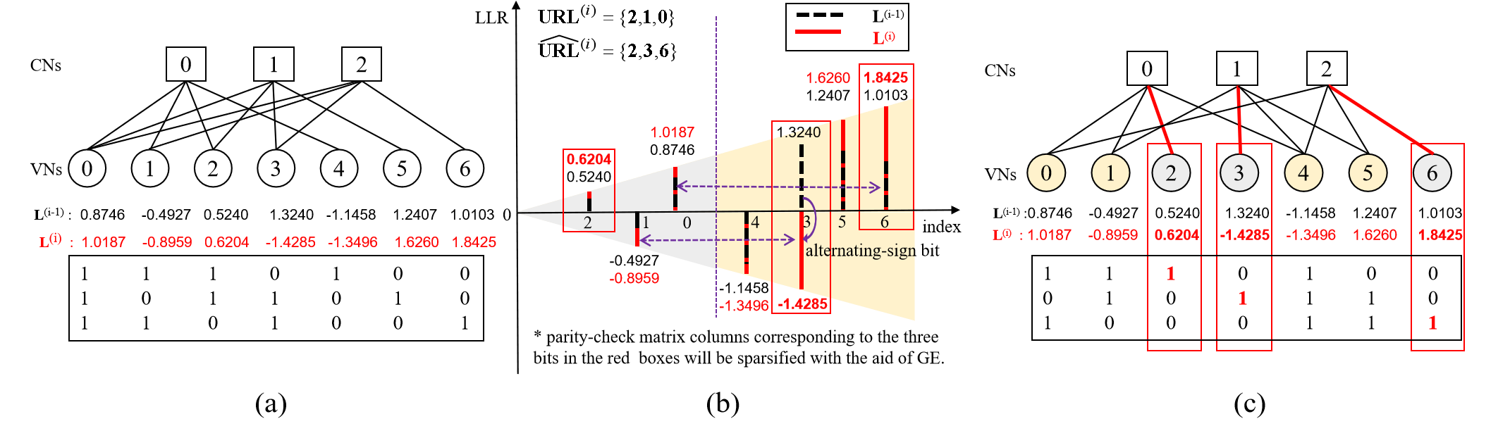
Figure 2: Illustration of the proposed PUM for a (7, 4)-Hamming code and $\rho=2$: (a) TG and parity-check matrix before GE; (b) How PUM is carried out; (c) TG and parity-check matrix after GE.

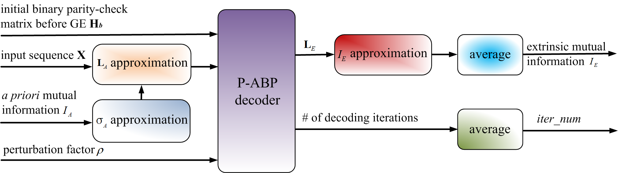
Figure 3: Extrinsic information analysis for perturbation factor $\rho$ of the proposed P-ABP decoder.

Input: $\mathbf{L}^{(i)}$, $\mathbf{L}^{(i-1)}$;

Output: Refined bit index set $\widehat{\mathbf{URL}}^{(i)}$ for sparsification of their parity-check columns.

1

2Step 1: Select $\rho$ using off-line extrinsic information analysis.

3Step 2: Record the LLR signs and absolute values before and after each decoding iteration;

4Step 3: Identify those bits from $\textbf{RL}^{(i)}$ with LLR sign changes and arrange their indices in descending order of amplitudes in $\mathbf{Z}^{(i)}=\{z_{1}^{(i)},z_{2}^{(i)},\cdots,z_{g}^{(i)}\ |\ g\leq K\}$;

5Step 4: Select $\rho$ bits and denote their index set by $\widehat{\mathbf{URL}}_{2}^{(i)}$:

6if $g\geq\rho$ then

7      choose the first $\rho$ entries from $\mathbf{Z}^{(i)}$ to generate $\widehat{\mathbf{URL}}_{2}^{(i)}$;

8

9else if $0<g<\rho$ then

10      choose all the alternating-sign bits from $\mathbf{Z}^{(i)}$, and then randomly choose $\rho-g$ bits from $\mathbf{URL}_{2}^{(i)}\bigcup\{\mathbf{RL}^{(i)}\setminus\mathbf{Z}^{(i)}\}$ to generate $\widehat{\mathbf{URL}}_{2}^{(i)}$;

11

12else

13      randomly choose $\rho$ bits from $\mathbf{URL}_{2}^{(i)}\bigcup\mathbf{RL}^{(i)}$ to generate $\widehat{\mathbf{URL}}_{2}^{(i)}$;

14

Step 5: Generate the new refined bit index set as $\widehat{\mathbf{URL}}^{(i)}=\mathbf{URL}_{1}^{(i)}\bigcup\widehat{\mathbf{URL}}_{2}^{(i)}$.

Algorithm 1 SubAlg-1: Proposed PUM Algorithm

Fig. 2 illustrates the PUM process by employing a (7, 4)-Hamming code as a simple example, where $N=7$, $M=3$, and the perturbation factor is assumed to be $\rho=2$. Fig. 2 (a) shows its TG, parity-check matrix and LLRs at the $i$-th iteration $\mathbf{L}^{(i)}$ and the $(i-1)$-th iteration $\mathbf{L}^{(i-1)}$. Fig. 2 (b) describes how the perturbation is carried out. Firstly, ${\bf{L}}^{(i)}$ are sorted in an ascending order according to the amplitudes. In this example, $\mathbf{URL}^{(i)}=\left\{2,1,0\right\}$, $\mathbf{URL}^{(i)}_{1}=\left\{2\right\}$, $\mathbf{URL}^{(i)}_{2}=\left\{1,0\right\}$, and $\mathbf{RL}^{(i)}=\left\{4,3,5,6\right\}$. Secondly, we detect the bits with alternating signs in $\mathbf{RL}^{(i)}$ based on $\mathbf{L}^{(i)}$ and $\mathbf{L}^{(i-1)}$, and then put their indices in set $\mathbf{Z}^{(i)}$. In Fig. 2 (b), only bit $v_{3}$ has LLRs with reversed signs during the latest two iterations, thus $\mathbf{Z}^{(i)}=\left\{3\right\}$. Since the number of bits with alternating signs is one, which is smaller than $\rho$, then one bit, say $v_{6}$, is randomly selected from $\mathbf{URL}_{2}^{(i)}\bigcup\{\mathbf{RL}^{(i)}\setminus\mathbf{Z}^{(i)}\}$. Therefore, we have $\widehat{\mathbf{URL}}_{2}^{(i)}=\left\{3,6\right\}$. Finally, the refined bit index set whose corresponding parity-check columns will be sparsified can be written as $\widehat{\mathbf{URL}}^{(i)}=\mathbf{URL}^{(i)}_{1}\bigcup\widehat{\mathbf{URL}}^{(i)}_{2}=\left\{2,3,6\right\}$. In Fig. 2 (c), GE is implemented, where the bits in $\widehat{\mathbf{URL}}^{(i)}$ are mapped to the sparse part of $\mathbf{\bar{H}}_{b}^{(i)}$.

III-A3 Perturbation Factor $\rho$

In this subsection, we propose an extrinsic information analysis method to find a good perturbation factor $\rho$. For a given initial binary parity-check matrix $\mathbf{H}_{b}$ and a priori mutual information $I_{A}$, the purpose here is to find a good $\rho$ which leads to the maximum extrinsic information $I_{E}$ as well as the smallest average iteration number $iter\_{num}$. Note that the conventional EXIT chart analysis [37] generally assumes a fixed Tanner graph. In our proposed P-ABP decoder, however, the Tanner graph changes according to the obtained LLRs over different BP iterations. In order to conduct the extrinsic information analysis, we treat the whole P-ABP decoder as a black box (as shown in Fig. 3), and do not care how the extrinsic information is transferred among different nodes in the intermediate parity-check matrices during the BP iterations. We only evaluate the resultant extrinsic information $I_{E}$ and $iter\_{num}$ after the decoding process. Finally, the $\rho$ with the maximum $I_{E}$ and the smallest $iter\_{num}$ is selected for a certain $I_{A}$.

Fig. 3 shows the signal processing flow of extrinsic information analysis. For a given input sequence $\mathbf{X}$ and $I_{A}$, a priori LLR $\mathbf{L}_{A}$ is generated to feed into the P-ABP decoder with a certain $\rho$ for extrinsic information analysis. First, the standard deviation $\sigma_{A}$ of $I_{A}$ is approximated as [38]

$$\sigma_{A}=J^{-1}(I_{A})\approx\left(-\frac{1}{H_{1}}\log_{2}\left(1-I_{A}^{\frac{1}{H_{3}}}\right)\right)^{\frac{1}{2H_{2}}},$$ (17)

where $H_{1}=0.3073$, $H_{2}=0.8935$, and $H_{3}=1.1064$. Then, the a priori LLR $\mathbf{L}_{A}$ can be estimated with the approximation method as [39]

$$\mathbf{L}_{A}=\frac{\sigma^{2}_{A}}{2}(2\mathbf{X}-1)+\sigma_{A}\mathbf{L}_{0},$$ (18)

where $\sigma^{2}_{A}$ is the variance of $I_{A}$, and $\mathbf{L}_{0}$ denotes the noise term, which is a sequence with the initial distribution of $\mathcal{N}(0,1)$. However, the noise term is expected to have the standard deviation of $\sigma_{A}$, thus $\mathbf{L}_{0}$ is multiplied by $\sigma_{A}$.

Finally, $I_{E}$ is approximated by the extrinsic LLR ($\mathbf{L}_{E}$) of the proposed P-ABP decoder [40]

$$\begin{split}I_{E}(L;X)=&1-\mathbf{E}\left\{\log_{2}(1+e^{-\mathbf{L}_{E}})\right\}\\ \approx&1-\frac{1}{N}\sum_{n=1}^{N}\log_{2}\left(1+e^{x_{n}l_{n}}\right)\\ \approx&1-\frac{1}{N}\sum_{n=1}^{N}\tilde{H}_{b}(P_{e_{n}}),\end{split}$$ (19)

where $l_{n}$ denotes the $n$-th element of $\mathbf{L}_{E}$, i.e., the LLR value of the $n$-th bit $x_{n}$, $P_{e_{n}}$ is the probability of $x_{n}\cdot\text{sgn}(l_{n})=-1$, i.e.,

$$P_{e_{n}}=\frac{e^{+\frac{|l_{n}|}{2}}}{e^{+\frac{|l_{n}|}{2}}+e^{-\frac{|l_{n}|}{2}}},$$

and $\tilde{H}_{b}$ denotes the binary entropy function:

$$\tilde{H}_{b}(P_{e_{n}})=-P_{e_{n}}\cdot\log_{2}(P_{e_{n}})-(1-P_{e_{n}})\cdot\log_{2}(1-P_{e_{n}}).$$

Fig. 4 shows an example of extrinsic information analysis for the perturbation factor $\rho$ with (127, 92)-BCH code. Specifically, in Fig. 4, two good values of $\rho$ for $I_{A}=0.75$ and $I_{A}=0.82$ are found to be 1 and 3, respectively, both of which give rise to the maximum $I_{E}$ and the smallest $iter\_num$. Moreover, the advantages of PUM aided ABP on both the extrinsic information and convergence speed can be observed in Fig. 4 for all $i_{\max}\in\{50,500,2000,4000\}$.

The proposed extrinsic information analysis can be carried out off-line and provides a simple but effective method to select the perturbation factor for the decoder.

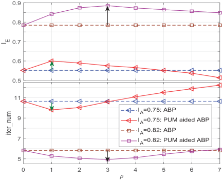
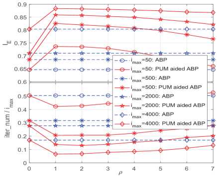
Figure 4: Extrinsic information analysis for finding good perturbation factor $\rho$ of (127, 92)-BCH code: (a) with $I_{A}\in\{0.75,0.82\}$ and $i_{\max}=20$; (b) with $I_{A}=0.75$ and $i_{\max}\in\{50,500,2000,4000\}$.

III-B P-ABP with Partial Layered Scheduling (PL-P-ABP)

III-B1 Layered Scheduling for HDPC Matrix

As introduced in Section I, for LDPC codes, both the shuffled BP and the layered BP have convergence rates twice faster than the flooding BP by timely propagating the latest updated messages. However, due to the special structure of parity-check matrix ${\bf{\bar{H}}}_{b}^{(i)}$ after GE, the flooding, shuffled and layered based ABP exhibit different performances in HDPC codes, compared to LDPC codes.

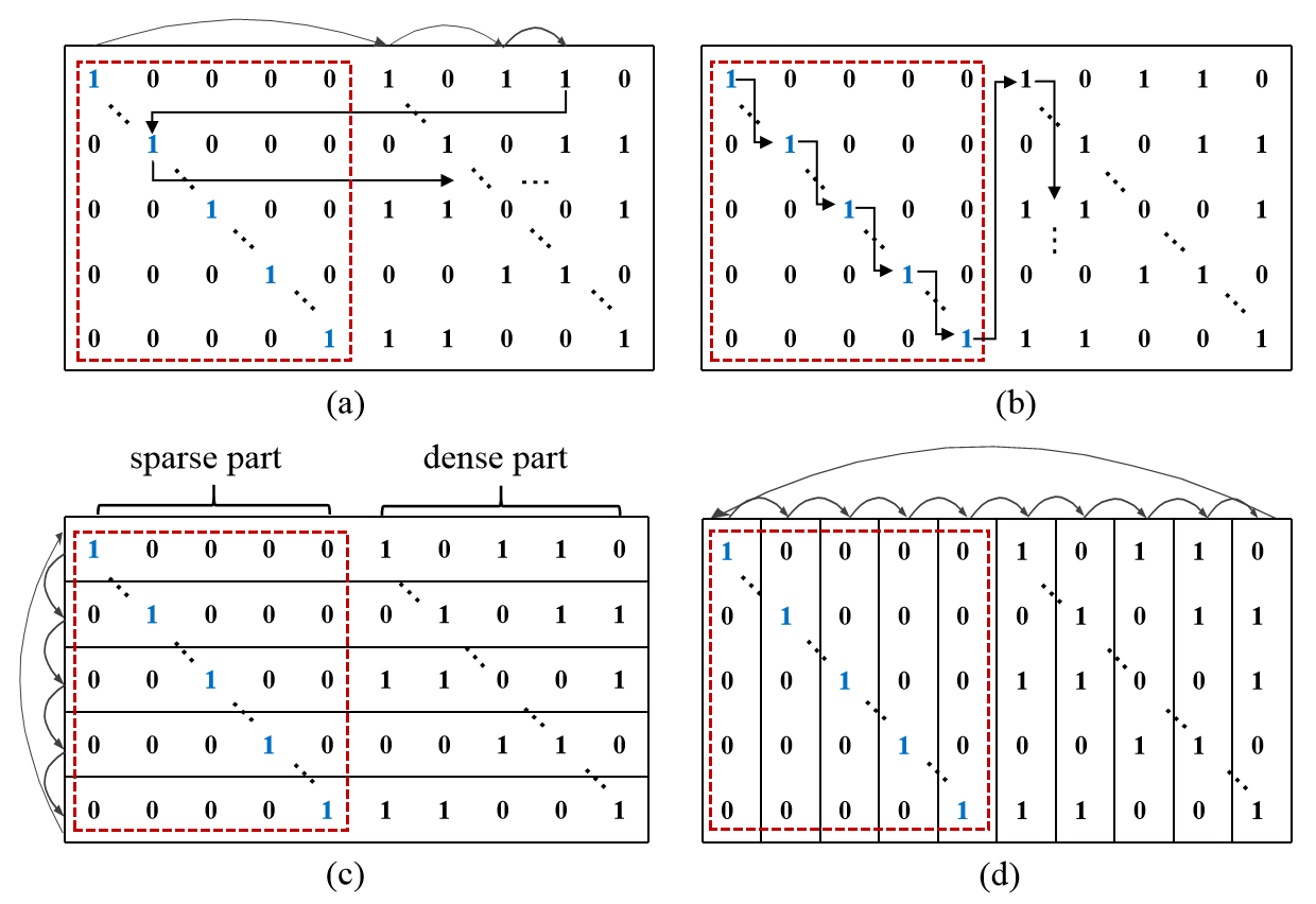
Figure 5: Schematic diagrams of ABP algorithms based on different scheduling strategies: (a) C2V update of flooding ABP (Phase 1); (b) V2C update of flooding ABP (Phase 2); (c) C2V and V2C updates of layered ABP; (d) C2V and V2C updates of shuffled ABP.

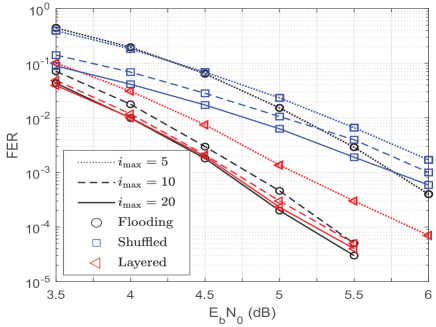
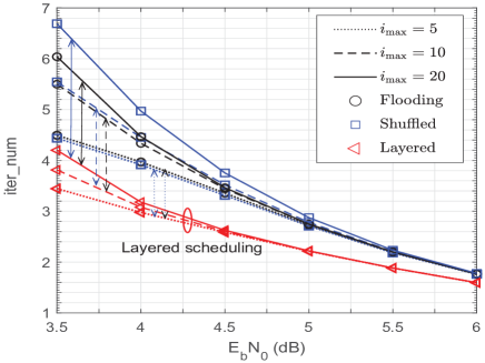
Figure 6: Performance comparison of different scheduling schemes for ABP with (31, 25)-RS code: (a) FER performance; (b) Average iteration number required to achieve FER shown in Fig. 6.

Fig. 5 shows the schematic diagrams of the ABP algorithms with different scheduling strategies. In each ABP iteration, the original parity-check matrix ${\bf{H}}_{b}$ of RS or BCH codes is transformed into a systematic matrix, i.e., ${\bf{\bar{H}}}_{b}^{(i)}$, where the diagonal sub-matrix (shown within the red dashed rectangle) and the complementary sub-matrix are called the sparse part and the dense part of the transformed matrix, respectively. Fig. 5(a) and Fig. 5(b) show the C2V and V2C message updating of flooding ABP, respectively; Fig. 5(c) and Fig. 5(d) individually describe the layered and shuffled ABP. As seen in Fig. 5(c), both the C2V and V2C updates of the layered ABP are similar to the row-by-row C2V update of flooding ABP (see arrows shown in Figs. 5(a) and 5(c)). In each row of the layered scheduling iteration, all the C2V and V2C messages of the neighboring VNs can be updated, including the sparse part and the dense part. On the other hand, both the C2V and V2C updates of the shuffled ABP in Fig. 5(d) are similar to the column-by-column V2C update of flooding ABP (see arrows shown in Figs. 5(b) and 5(d)). Again, it is stressed that for each VN in the sparse part, there is one neighboring CN only. Due to the column-by-column iteration pattern, there is no V2C update in the sparse part for both the flooding and shuffled ABP according to (6); and only once C2V update to the single VN in each column of the sparse part for the shuffled ABP according to (8).

Fig. 6 shows the error correction performances and the convergence rates of different scheduling based ABP algorithms with maximum iteration numbers $i_{\max}$ of 5, 10, and 20, respectively. As seen from both Fig. 6 and Fig. 6, the layered ABP (red lines) can achieve similar or better FER performance with lesser iteration counts, compared to the other two scheduling algorithms. Its superiority is more noticeable in low SNR region as $i_{\max}$ increases. The FER performance of shuffled scheduling is worse than the other two scheduling strategies when $i_{\max}$ is small.

Based on the above analysis, we adopt the layered scheduling as it enjoys the fastest convergence rate and similar or better error correction performance within a certain $i_{\max}$. Accordingly, the extrinsic LLR in (11) is rewritten as

$$\begin{split}L_{\text{ext}}^{(i)}({v_{n}})\!=\!\sum\limits_{\begin{subarray}{c}c_{m}\in{\cal{M}}\left(v_{n}\right)\\ c_{j}<c_{m}\end{subarray}}\!{2{{\tanh}^{-1}}\left({\prod\limits_{v_{j}\in{\cal{N}}\left(c_{m}\right)\backslash v_{n}}{\tanh\left({\frac{{{L^{(i)}}({v_{j}})}}{2}}\right)}}\right)}\\ \!+\!\sum\limits_{\begin{subarray}{c}c_{m}\in{\cal{M}}\left(v_{n}\right)\\ c_{j}>c_{m}\end{subarray}}\!{2{{\tanh}^{-1}}\left({\prod\limits_{v_{j}\in{\cal{N}}\left(c_{m}\right)\backslash v_{n}}{\tanh\left({\frac{{{L^{(i-1)}}({v_{j}})}}{2}}\right)}}\right)}\end{split}.$$ (20)

III-B2 Partial updating

In BP based decoding, a large number of VNs may converge with large LLRs after a few iterations. For LDPC codes, one may adopt a forced convergence strategy to significantly reduce the decoding complexity with negligible compromise in error correction performance [41]. For HDPC codes with a large number of short cycles, some edges of short cycles may be skipped by partial updating, which is helpful to obtain an enhanced error correction performance [28]. However, straightforward application of the partial updating strategy of e-Flooding schedule in[28] is not optimal for HDPC codes.

In this work, we propose an improved partial updating strategy combined with layered scheduling for HDPC codes to pursue both fast convergence rate and enhanced error correction performance. In our proposed partial updating strategy, the edge-state vector $\mathcal{E}$ is iteratively updated to determine which edges should be updated, where

$$\mathcal{E}=\{\varepsilon_{m,n}\ |\ 1\leq m\leq M,v_{n}\in\mathcal{N}\left(c_{m}\right)\},$$ (21)

and $\varepsilon_{m,n}\in\{0,1\}$. $\varepsilon_{m,n}=1$ indicates that the edge $\vec{e}_{m,n}$ has not converged, hence will be updated in the next iteration, and vice versa. The improved edge-state update criteria can be described as follows: First, all the edges related with unsatisfied syndromes need to be updated. Next, if the related syndrome $s_{c_{m}}^{(i)}$ is satisfied, but the minimum LLR magnitude $\eta_{c_{m}}$ of the connected VNs is smaller than a reliability threshold $\mathcal{T}$, only the edges with indices belong to $\widehat{\mathbf{URL}}^{(i)}$ are updated in the next iteration. The reliability threshold $\mathcal{T}$ is a function of the average CN degree $\bar{d}_{c}$ which is shown in [28]. Different from e-Flooding [28], the amplitude comparison is not required in our solution to decide which VNs need to be updated in the i-th iteration. Only VNs in $\widehat{\mathbf{URL}}^{(i)}$ are selected for updating.

The detailed algorithm of the proposed PL-P-ABP is shown in Algorithm 1. In each iteration of Algorithm 1, PUM and GE are implemented first from Steps 3 to 5; then the edge-state vector $\mathcal{E}$ is updated from Steps 6 to 14; finally the partial layered updating is implemented according to $\mathcal{E}$, followed by LLRs updating and termination judgment.

1 Initialize ${\bf{L}}^{(0)}=\mathbf{L}_{\text{ch}}$, $i_{\max}$;

2 for $i=0:i_{{\max}}-1$ do

3       Sorting ${\bf{L}}^{(i)}$, generate $\mathbf{URL}^{(i)}$ and $\mathbf{RL}^{(i)}$ ;

4       Execute PUM (SubAlg-1), return $\widehat{\mathbf{URL}}^{(i)}$ ;

5       Execute GE on $\mathbf{H}_{b}$, return $\mathbf{\overline{H}}^{(i)}_{b}$ ;

6       Update the edge-state vetor $\mathcal{E}$:      

7           Set $\mathcal{E}=\{\varepsilon_{m,n}=0|1\leq m\leq M,v_{n}\in\mathcal{N}(c_{m})\}$ ;

8       for $\forall\ c_{m},1\leq m\leq M$  do

9             if $s_{c_{m}}^{(i)}\neq 0$  then

10                  for $\forall\ v_{n}\in\mathcal{N}(c_{m})$ do

11                        $\varepsilon_{m,n}=1$ ;

12                  

13            

14            if $s_{c_{m}}^{(i)}=0\ \&\ \eta_{c_{m}}<\mathcal{T}$  then

15                  for $\forall\ v_{n}\in\mathcal{N}(c_{m})\cap\widehat{\mathbf{URL}}^{(i)}$ do

16                         $\varepsilon_{m,n}=1$ ;

17                        

18                  

19            

20      Execute partial layered updating:      

21           for $m=1:M$ do

22             for $\forall v_{n}\in\mathcal{N}(c_{m})$ do

23                   if $\varepsilon_{m,n}=1$ then

24                         update $C_{c_{m}\rightarrow v_{n}}^{(i)}$ by (5);

25                         update $V_{v_{n}\rightarrow c_{m}}^{(i)}$ by (9);

26                        

27                  

28            

29      Update ${\bf{L}}^{(i)}$ by (20) and (12);

30       Hard decision on ${\bf{L}}^{(i)}$ to yield $\mathbf{\hat{c}}^{(i)}$ ;

31       if $\{s_{c_{m}}^{(i)}=0|1\leq m\leq M\}$ then

32            Terminate decoding;

33      Proceed to Step $\mathbf{3}$ ;

34      

35Return $\mathbf{\hat{c}}^{(i)}$ ;

End

Algorithm 2 Algorithm 1: P-ABP with partial layered scheduling (Proposed PL-P-ABP)

III-B3 Variation of PL-P-ABP for Product Codes

The product code, as a special concatenation of some linear block codes, such as BCH and RS codes, is a widely recognized technique to attain multiplied minimum distance. Constructions of a product code can be found in [42, 43, 13]. Consider the product code $\mathfrak{P}=\mathfrak{C}^{1}\times\mathfrak{C}^{2}$ with two component codes $\mathfrak{C}^{j}$ with parameters of $(n_{j},k_{j},d_{j}),j=1,2$, where $n_{j}$, $k_{j}$ and $d_{j}$ denote the codeword length, the message length, and the minimum distance, respectively. The codeword length of $\mathfrak{P}$ is $n_{p}=n_{1}\times n_{2}$, the information bit length is $k_{p}=k_{1}\times k_{2}$, and the minimum distance is $d_{p}=d_{1}\times d_{2}$.

TAB [24] is a turbo-oriented ABP decoding for product codes, in which a parity-check matrix adaptation is moved outside of the ABP decoding loop with very few maximum local iteration number (usually 3 to 5). Moreover, the damping factor is not adopted in TAB. The effect of extrinsic LLR is reduced during the a posteriori LLR computation process [42].

In this work, the proposed PL-P-ABP is further modified to adapt to the turbo iterative decoding of product codes. Such a modified decoding scheme, called PL-P-ABP-P, is specified in Algorithm 2, where $i_{\text{global}}$ denotes the maximum global iteration (i.e., outer loop iteration) number, and $i_{\text{local}}$ denotes the maximum local iteration number of PL-P-ABP. $NumSucc$ is the counter of successful decoded rows or columns in each half global iteration, which is used for termination decision. Note that PUM and GE are moved outside of local PL-P-ABP decoding loop. Furthermore, considering the small number of local iterations, the LLR updating in global iterations adopts the following rule to prevent error propagation:

$${\mathbf{L}^{(i+1)}=\begin{cases}\mathbf{L}^{(i)},&\mbox{if $\sum S_{c_{m}}^{(i)}=0$ };\\ \mathbf{L}_{\text{ch}},&\mbox{otherwise}\end{cases},}$$ (22)

where $S_{c_{m}}^{(i)}$ is the syndrome of $m$-th CN of component codes. LLRs are updated only if all the checks of component codes in a certain row or column are satisfied; otherwise, the initial channel information $\mathbf{L}_{\text{ch}}$ will be used in the global iterations.

1 Initialize $n_{1}$, $n_{2}$, ${\mathbf{L}}^{(0)}=\mathbf{L}_{\text{ch}}$, $NumSucc=0$ ;

2 Set $i_{\text{global}}$, $i_{\text{local}}$ ;

3 for $i=0:i_{\text{global}}-1$ do

4       for $row=0:n_{1}-1$ do

5            Sorting $\mathbf{L}^{(i)}(row,:)$, generate $\mathbf{URL}^{(i)}$ and $\mathbf{RL}^{(i)}$ ;

6             Execute PUM (SubAlg-1), return $\widehat{\mathbf{URL}}^{(i)}$;

7             Execute GE on $\mathbf{H}_{b}$, return $\overline{\mathbf{H}}_{b}^{(i)}$ ;

8             for $j=0:i_{\text{local}}-1$ do

9                   Execute Algorithm 1;

10            Hard decision to yield $\mathbf{\hat{c}}^{(i)}(row,:)$ ;

11             if $\sum S_{c_{m}}^{(i)}=0$ then

12                  $NumSucc=NumSucc+1$ ;

13            Update LLR: $\mathbf{L}^{(i+1)}(row,:)$ by (22) ;

14            

15      if  $NumSucc=n_{1}$ then

16            Terminate decoding, proceed to Step $\mathbf{29}$;

17      $NumSucc=0$;

18      

19      for $col=0:n_{2}-1$ do

20            Sorting $\mathbf{L}^{(i)}(:,col)$, generate $\mathbf{URL}^{(i)}$ and $\mathbf{RL}^{(i)}$ ;

21             Execute PUM (SubAlg-1), return $\widehat{\mathbf{URL}}^{(i)}$;

22             Execute GE on $\mathbf{H}_{b}$, return $\overline{\mathbf{H}}_{b}^{(i)}$ ;

23             for $j=0:i_{\text{local}}-1$ do

24                   Execute Algorithm 1;

25            Hard decision to yield $\mathbf{\hat{c}}^{(i)}(:,col)$ ;

26             if $\sum S_{c_{m}}^{(i)}=0$ then

27                  $NumSucc=NumSucc+1$ ;

28            Update LLR: $\mathbf{L}^{(i+1)}(:,col)$ by (22) ;

29            

30      if  $NumSucc=n_{2}$ then

31            Terminate decoding, proceed to Step $\mathbf{29}$;

32      $NumSucc=0$;

33       Proceed to Step $\mathbf{4}$ ;

34      

35Return $\mathbf{\hat{c}}^{(i)}$ ;

End

Algorithm 3 Algorithm 2: Variation of PL-P-ABP for product codes (Proposed PL-P-ABP-P)

1 Initialize ${\bf{L}}^{(0)}=\mathbf{L}_{\text{ch}}$, $C2V_{\text{update}}=0$, $i_{\max}$, $total\_edges$;

2 for $i=0:i_{{\max}}-1$ do

3       Sorting ${\bf{L}}^{(i)}$, generate $\mathbf{URL}^{(i)}$ and $\mathbf{RL}^{(i)}$ ;

4       Execute PUM (SubAlg-1), return $\widehat{\mathbf{URL}}^{(i)}$ ;

5       Execute GE on $\mathbf{H}_{b}$, return $\mathbf{\overline{H}}^{(i)}_{b}$ ;

6       Execute layered scheduling once for bits in $\widehat{\mathbf{URL}}^{(i)}$:                  

7      for $m=1:M$ do

8             Generate and propagate $C_{c_{m}\rightarrow v_{n}}^{(i)}$ with (5);

9      

10      Execute D-SVNF scheduling:                        while $\left(C2V_{\text{update}}<total\_edges-M\right)$ do

11            

12            if all $\{u_{n}=1,1\leq n\leq N\}$  then

13                   Reset $\{u_{n}=0$, $1\leq n\leq N\}$ ;

14            

15            Select $v_{p}:u_{p}=0,u_{i}=1,\forall i<p$. Set $u_{p}=1$ ;

16             for $c_{m}\in\mathcal{M}\left(v_{p}\right),s_{c_{m}}=1,v_{n}\in\mathcal{N}\left(c_{m}\right)\setminus v_{p}$  do

17                   Compute $R^{(i)}\left({c_{m}\rightarrow v_{n}}\right)$ with (23);

18            

19            Find $R^{(i)}\left({c_{i}\rightarrow v_{j}}\right)={\max}\{R^{(i)}\left({c_{m}\rightarrow v_{n}}\right)|$

20             $c_{m}\in\mathcal{M}\left(v_{p}\right),v_{n}\in\mathcal{N}\left(c_{m}\right)\setminus v_{p}\}$ ;

21            

22            Generate and propagate $C_{c_{i}\rightarrow v_{j}}^{(i)}$ with (5) ;

23             $C2V_{\text{update}}=C2V_{\text{update}}+1$ ;

24             Set $R^{(i)}\left(c_{i}\rightarrow v_{j}\right)=0$;

25            

26            for $c_{a}\in\mathcal{M}\left(v_{j}\right)\setminus c_{i}$ do

27                   Generate and propagate $V_{v_{j}\rightarrow c_{a}}^{(i)}$ with (9);

28                  

29            if $u_{j}=1$ then

30                  Proceed to Step 4 ;

31            else

32                  Set $v_{p}=v_{j}$, $u_{p}=1$. Proceed to Step 4;

33            

34      Update ${\bf{L}}^{(i)}$ by (20) and (12);

35       Hard decision on ${\bf{L}}^{(i)}$ to yield $\mathbf{\hat{c}}^{(i)}$ ;

36       if $\{s_{c_{m}}^{(i)}=0|1\leq m\leq M\}$ then

37            Terminate decoding;

38      Proceed to Step $\mathbf{3}$ ;

39      

40Return $\mathbf{\hat{c}}^{(i)}$ ;

End

Algorithm 4 Algorithm 3: P-ABP with hybrid dynamic scheduling (Proposed HD-P-ABP)

TABLE II: Complexity analysis of fixed and dynamic scheduling based algorithms (per iteration)

Scheme	Code	Algorithm	V2C update	C2V update	Residual computation	Real-value comparison
fixed	RS/BCH codes	ABP [19]	$E$	$E$	$0$	$0$
		e-Flooding ABP [28]	$\leq E$	$\leq E$	$0$	$\psi$
		PL-P-ABP (Proposed)	$\leq E$	$\leq E$	$0$	$\leq N+K(K-1)/2$
	product codes	TAB [24]	$n_{1}E_{2}+n_{2}E_{1}$	$n_{1}E_{2}+n_{2}E_{1}$	$0$	$0$
		PL-P-ABP-P (Proposed)	$\leq(n_{1}E_{2}+n_{2}E_{1})$	$\leq(n_{1}E_{2}+n_{2}E_{1})$	$0$	$\leq n_{1}(n_{2}+k_{2}(k_{2}-1)/2)$ $+n_{2}(n_{1}+k_{1}(k_{1}-1)/2)$
dynamic	RS/BCH codes	LRBP [35]	$\left(\bar{d_{v}}-1\right)E$	$E$	$\left(\bar{d_{v}}-1\right)\left(\bar{d_{c}}-1\right)E$	$\left(\bar{d_{c}}-1\right)E$
		DP-RBP [36]	$\left(\bar{d_{v}}-1\right)E$	$E$	$\left(\bar{d_{v}}-1\right)\left(\bar{d_{c}}-1\right)E$	$\left(\bar{d_{c}}-1\right)E$
		HD-P-ABP (Proposed)	$\left(\bar{d_{v}}-1\right)E$	$E$	$\leq\left(\bar{d_{v}}-1\right)\left(\bar{d_{c}}-1\right)E$	$\leq\left[\bar{d_{v}}\left(\bar{d_{c}}-1\right)-1\right]E$

• $E$: total edges in the TG $\bar{d_{v}}$: average VN degree $\bar{d_{c}}$: average CN degree $\psi$: see [28]

• $n_{1},n_{2},k_{1},k_{2},E_{1},E_{2}$: codeword lengths, message lengths, and total edges in the TG of product component codes

III-C P-ABP with Hybrid Dynamic Scheduling (HD-P-ABP)

Partial layered scheduling is a form of fixed scheduling, which means that the scheduling order/sequence can be predetermined off-line. Compared with fixed scheduling, dynamic scheduling can further improve the convergence rate, by determining the scheduling order on-the-fly during decoding runtime. The main idea of dynamic scheduling is to first update the message associated with the largest LLR residual (then the second largest and so on). Formal definition of “LLR residual” can be found in (23). This will allow the decoder to focus on the part of TG that has not converged. Moreover, dynamic decoding has potential to circumvent trapping sets in TG and hence improve the error correction performance [29].

However, dynamic scheduling may lead to certain types of greedy groups, each consisting of a few CNs or VNs which excessively consuming the computing resources. A greedy group is called a myopic error if it is formed by a small number of CNs [29]. The greedy group formed by certain VNs may also result in some silent-variable-nodes which never have a chance to be updated in the decoding process [30]. Although some improved dynamic schemes have been proposed to prevent those greedy groups for LDPC codes [30, 33, 29], little is understood on how to prevent greedy groups for HDPC codes. The LRBP for RS codes in [35] can efficiently avoid myopic error by sequentially updating the C2V message, but may not be able to prevent the silent-variable-nodes. Motivated by these issues, we propose a hybrid dynamic scheduling for HDPC codes to circumvent both types of greedy groups.

Our proposed HD-P-ABP is a hybrid schedule that combines layered scheduling and D-SVNF scheme. The main idea of HD-P-ABP is that the layered scheduling is applied only once for the unreliable bits in $\widehat{\mathbf{URL}}^{(i)}$ before the D-SVNF scheduling. By doing so, one can prevent both the myopic error by layered scheduling, and the silent-variable-nodes by D-SVNF scheduling. Moreover, it provides one more chance of C2V message updating for the unreliable bits by layered scheduling. Those updated messages before the second iteration are almost independent and reliable for a HDPC code with large number of short cycles [44].

The details of HD-P-ABP are presented in Algorithm 3 with some definitions given first. The C2V message residual $R^{(i)}\left({c_{m}\rightarrow v_{n}}\right)$ is defined as

$$R^{(i)}\left({c_{m}\rightarrow v_{n}}\right)=\left|C_{c_{m}\rightarrow v_{n}}^{(i-1)}-C_{c_{m}\rightarrow v_{n}}^{(i)}\right|,$$ (23)

where $C_{c_{m}\rightarrow v_{n}}^{(i-1)}$ denotes the C2V message at the $(i-1)$-th iteration. To prevent the silent-variable-nodes, a binary vector $\mathbf{u}=\{u_{n},1\leq n\leq N\}$ is set to record the update states of VNs, where $u_{n}=1$ indicates that the variable node $v_{n}$ has been updated and hence should not be updated again in the current iteration. The variable $total\_edges$ represents the total edges in the TG, and $C2V_{\text{update}}$ is used to count the C2V update numbers, which should not be larger than $total\_edges$.

In Algorithm 3, PUM and GE are implemented first. From Steps 6 and 7, the C2V messages of unreliable bits in $\widehat{\mathbf{URL}}^{(i)}$ are updated once with layered scheduling. By doing so, all the CNs have been updated at least once to prevent the myopic error. Then D-SVNF scheduling is implemented from Steps 8 to 24. It is noted that D-SVNF allows a dynamic updating order of VNs, which can not only get rid of the silent-variable-nodes, but also prioritize the message updating of the most probably erroneous VNs which are connected with those CNs with unsatisfied syndromes, thus resulting in a faster decoding convergence rate [33].

IV Complexity Analysis

In this section, the decoding complexities of the proposed and prior-art algorithms per decoding iteration are analyzed. Table II lists the total numbers of V2C and C2V message updates, residual computations, and real-value comparisons in a single decoding iteration. For product codes, “per iteration” means per global iteration. The real-value comparison is used to measure the scheduling complexity which can be realized in the hardware by a full-adder circuit [45]. For fair comparison, no HDD is considered to assist SDD in all the compared algorithms in Table II.

For fixed algorithms, ABP [19] needs $E$ numbers of V2C and C2V message updates, where $E$ denotes the number of total edges in TG. Both e-Flooding ABP [28] and the proposed PL-P-ABP require fewer numbers of V2C/C2V updates than ABP, owing to partial updating strategies. The real-value comparisons of e-Flooding ABP denoted as $\psi$ are used for identification of minimum-reliability VNs. The approximation of $\psi$ is specified in [28]. Compared with $\psi$, the real-value comparisons of proposed PL-P-ABP are quite simple, only involving $N$ numbers of sign comparison and $g(g-1)/2$ numbers of magnitude comparison in the PUM, where $g$ is the number of alternating-sign bits ($g\leq K$). As for product codes, since the component codes are iteratively decoded by local algorithms (i.e., local ABP for TAB, and local PL-P-ABP for PL-P-ABP-P), the overall V2C/C2V updates and real-value comparisons of TAB [24] and PL-P-ABP-P are linear combinations of those of local algorithms. Thus, the V2C and C2V updates of PL-P-ABP-P are less complex than TAB.

For dynamic algorithms, the proposed HD-P-ABP has the same V2C and C2V message update counts with LRBP [35] and DP-RBP [36], i.e., $\left(\bar{d_{v}}-1\right)E$ and $E$, respectively, where $\bar{d_{v}}$ denotes the average VN degree. Since LRBP and DP-RBP update CNs with a sequential order and a double-polling mechanism, respectively, which have fixed numbers of residual computation and real-value comparison, i.e., $\left(\bar{d_{v}}-1\right)\left(\bar{d_{c}}-1\right)E$ and $\left(\bar{d_{c}}-1\right)E$, respectively. However, the updating order of VNs in the proposed HD-P-ABP is dynamic, in that the residual computation and real-value comparison is implemented on-demand only for the CNs with unsatisfied syndromes (which are connected to the current updating VNs). Therefore, the proposed HD-P-ABP has less residual computational complexity than LRBP and DP-RBP. The real-value comparison of HD-P-ABP is less than $\left[\bar{d_{v}}\left(\bar{d_{c}}-1\right)-1\right]E$, which is comparable to that of LRBP and DP-RBP.

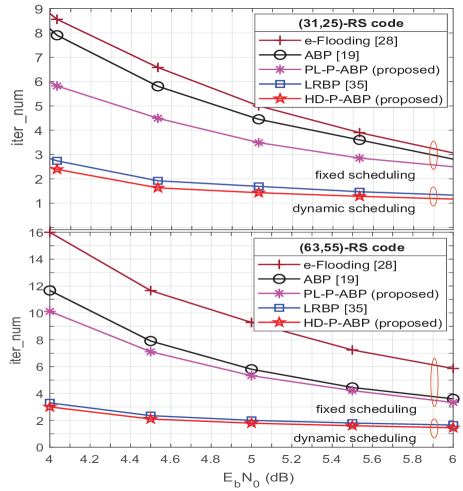
Figure 7: FER and decoding convergence comparisons for (31, 25)-RS code and (63, 55)-RS code with $i_{\max}=50$: (a) FER performance; (b) Average iteration number required to achieve FER shown in Fig. 7.

V Simulation results

In this section, we benchmark the performances of the proposed PL-P-ABP and HD-P-ABP algorithms for RS and BCH codes against the prior-art ABP algorithms, including traditional ABP in [19], LRBP in [35], DP-RBP in [36], and e-Flooding ABP in [28]. For product codes, the proposed PL-P-ABP-P is compared with the Chase-Pyndiah algorithm in [13], and TAB algorithm in [24].

V-A Performance Comparison for RS Codes

Two types of RS codes are considered for simulation, i.e., rate-0.80 (31, 25)-RS code and rate-0.87 (63,55)-RS code, both having high coding rates, short block lengths, and HDPC matrices with large numbers of short cycles. The maximum decoding iteration number is set to be $i_{\max}=50$, which follows the setting of [28].

Fig. 7 compares the FER performances and the average required iteration numbers ($iter\_num$) of different algorithms for RS codes. The green lines in Fig. 7 represent the lower bounds of the maximum likelihood (ML) decoding from [46] and [19], the purple lines show the performance of Berlekamp-Massey decoding algorithm [8]. For the fixed schemes, e-Flooding ABP achieves better error correction performance with a certain loss of convergence rate compared with ABP (due to the partial updating strategy). The proposed PL-P-ABP can further improve the average convergence rates of ABP by 22.76% for (31,25)-RS code and 18.5% for (63,55)-RS code, respectively, while maintaining an error rate performance comparable to that of e-Flooding ABP but about 0.3 dB gains over ABP at FER of $10^{-5}$. Both the two dynamic schemes have comparable rapid decoding convergence rates. The proposed HD-P-ABP can improve the convergence rate of ABP by 67%, while obtaining enhanced error rate performance about 0.5 dB and 0.3 dB gains over ABP and LRBP at FER of $10^{-5}$ for (31,25)-RS code, respectively.

We further bench mark the proposed dynamic scheme HD-P-ABP with LRBP [35] and DP-RBP [36] for (255,239)-RS code and (127,121)-RS code, which is shown in Fig. 8. Considering the long codeword length and high decoding complexity of (255,239) and (127,121) RS codes, the algebraic HDD is also incorporated into the proposed HD-P-ABP for faster decoding and enhanced error rate performances [35, 36]. As shown in Fig. 8, with a maximum iteration number of $i_{\max}=60$, the proposed HD-P-ABP can achieve about 0.5 dB and 0.1 dB of SNR gain over ABP and LRBP for (255,239)-RS code at FER=$10^{-3}$, respectively, and about 0.65 dB and 0.15 dB of SNR gain over ABP and DP-RBP for (127,121)-RS code at FER=$10^{-3}$, respectively. There are two main factors which contribute to the performance gains of the proposed HD-P-ABP, i.e., the proposed PUM strategy and the hybrid dynamic scheduling.

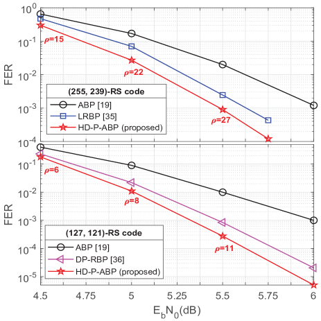
Figure 8: FER comparison for (255, 239)-RS code and (127, 121)-RS code with $i_{\max}=60$ and algebraic HDD assistance.

V-B Performance Comparison for BCH Codes

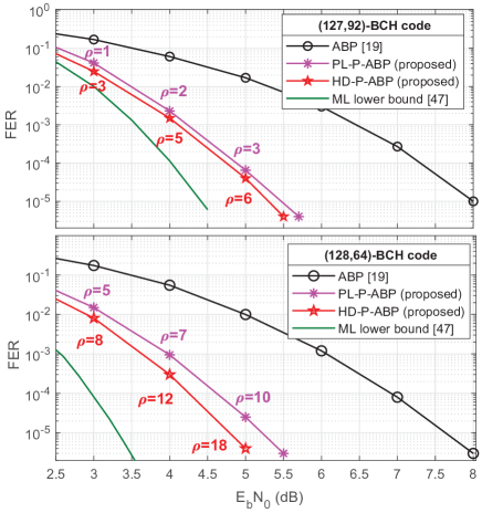
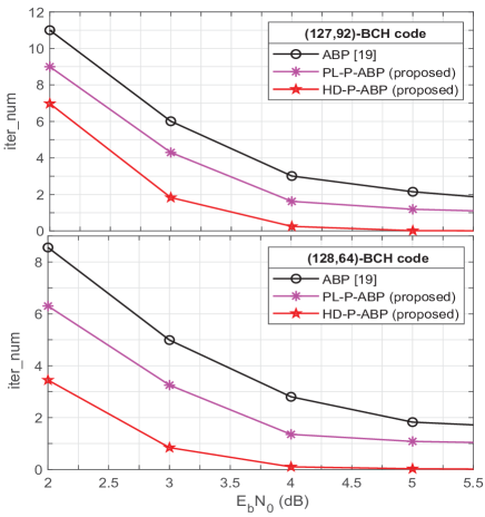
Figure 9: FER and decoding convergence comparisons for (127, 92)-BCH code and (128, 64)-BCH code with $i_{\max}=20$: (a) FER performance; (b) Average iteration number required to achieve FER shown in Fig. 9.

In this section, we apply the proposed algorithms to rate-0.72 (127, 92)-BCH code and rate-0.5 (128, 64)-BCH code, and compare them with the traditional ABP in [19]. The maximum iteration number is set to be $i_{\max}=20$ for FER convergence of the proposed algorithms.

Fig. 9 shows the FER and convergence rate comparisons for BCH codes. The green lines represent the ML simulation results from [47]. For (127, 92)-BCH code, PL-P-ABP and HD-P-ABP lead to 34.43% and 74.50% faster convergence rates compared with ABP, respectively; while for (128, 64)-BCH code, the average convergence rate improvements are severally 38.38% and 84.49%. Owing to their faster convergence rates, the proposed algorithms can achieve at least 2.25 dB gains over ABP at FER of $10^{-5}$ within a small iteration number. HD-P-ABP outperforms PL-P-ABP about 0.2-0.4 dB.

V-C Performance Comparison for Product Codes

We consider the rate-0.54 $(15,11)^{2}$-RS product code. The iteration numbers are set the same as that in [24], i.e., global iterations of $i_{\text{global}}=8$ and local iterations of $i_{\text{local}}=5$. Fig. 10 shows the bit error rates (BER) of compared algorithms. The green solid and dashed lines represent the Poltyrev tight bounds on ML soft decision decoding (ML-SDD) and ML hard decision decoding (ML-HDD), respectively, from [48] and [49]. The proposed PL-P-ABP-P achieves about 0.5 dB and 1.1 dB gains over TAB [24] and Chase-Pyndiah algorithm [13] at BER of $10^{-6}$, respectively. Moreover, the proposed PL-P-ABP-P is less than 0.5 dB from the tight bound of ML-SDD at BER of $10^{-6}$, which is a good result not attainable before. On the other hand, as shown in Table II, the proposed PL-P-ABP-P also has lower decoding complexity than TAB. Note that the local PL-P-ABP is repeatedly implemented in the global iterations of PL-P-ABP-P, leading to faster convergence rate than local ABP based TAB (as shown in Fig. 7). Thus, the superiority of PL-P-ABP-P on the decoding convergence rate over TAB follows.

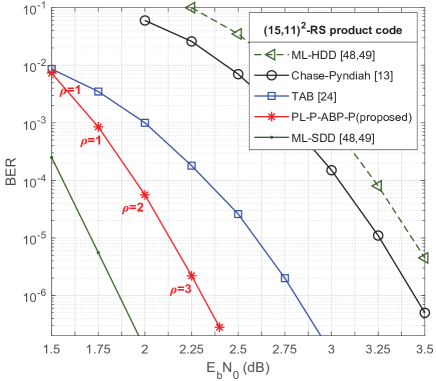
Figure 10: BER comparison of rate-0.54 $(15,11)^{2}$-RS product code with different decoding methods, where $i_{\text{global}}=8$, $i_{\text{local}}=5$ are set in [24] and the proposed PL-P-ABP-P.

VI Conclusion

This paper considers the SISO decoding of HDPC codes such as BCH codes, RS codes, and product codes using an adaptive belief propagation (ABP) algorithm. We have observed that the traditional ABP, which sparsifies the parity-check columns corresponding to the $M$ least reliable bits (where $M$ denotes the number of parity-check bits), may not be optimal. Our key idea, called Perturbed ABP (P-ABP), is to include a few unstable bits with large LLR magnitudes but incorrect signs in the parity-check matrix sparsification. We have proposed an off-line extrinsic information analysis method to search the proper number and the locations of these unstable bits.

We then augment the P-ABP with two novel scheduling schemes, namely, partial layered scheduling or hybrid dynamic scheduling resulting in PL-P-ABP (Algorithm 1) and HD-P-ABP (Algorithm 3), respectively. PL-P-ABP adopts layered scheduling and an improved partial updating strategy to skip unreliable message passing caused by some short cycles in HDPC codes, while HD-P-ABP adopts a hybrid usage of layered scheduling and D-SVNF to circumvent multiple types of greedy groups. To decode product code, we have extended PL-P-ABP to PL-P-ABP-P (Algorithm 2) in a non-trivial way to avoid error propagation between the horizontal and vertical decoding processes.

Our simulations have shown that PL-P-ABP and HD-P-ABP achieve gains of 2.25 dB and 2.75 dB, and convergence rate improvement of 38.38 % and 84.49% over the traditional ABP for the (128,64)-BCH code, respectively. Separately, the decoding performance of the proposed PL-P-ABP-P on $(15,11)^{2}$-RS product code is within 0.5 dB from the tight bound of ML decoding, which is much improved compared to Chase-Pyndiah decoding or TAB decoding.

The excellent decoding performance of proposed P-ABP algorithms do not come with higher computational complexity. As shown in Table II, the proposed algorithms have less or similar decoding complexities per iteration compared to the prior-art fixed or dynamic ABP algorithms. Coupled with the fewer iteration numbers required to achieve a particular FER (shown in Fig. 7 and 9), the proposed P-ABP decoders can be concluded to have lower overall computational complexity.

References

- [1] I. S. Reed and G. Solomon, “Polynomial codes over certain finite fields,” Journal of the Society for Industrial and Applied Mathematics, vol. 8, no. 2, pp. 300–304, Oct. 1960.
- [2] S. B. Wicker, Reed-Solomon Codes and Their Applications. Piscataway, NJ, USA: IEEE Press, 1994.
- [3] W.J.Gross, F. Kschischang, R. Koetter, and P. Gulak, “Applications of algebraic soft-decision decoding of Reed-Solomon codes,” IEEE Trans. Commun., vol. 54, no. 7, pp. 1224–1234, Jul. 2006.
- [4] C. Xu, Y. C. Liang, Y. L. Guan, and W. Leon, “Turbo product codes for mobile multimedia broadcasting with partial-time jamming,” IEEE Trans. Broadcast., vol. 53, no. 1, pp. 256–262, Mar. 2007.
- [5] J. V. Wonterghem, A. Alloum, J. J. Boutros, and M. Moeneclaey, “Performance comparison of short-length error-correcting codes,” in 2016 Symposium on Communications and Vehicular Technology (SCVT), Nov. 2016, pp. 1–6.
- [6] M. Shirvanimoghaddam and et al., “Short block-length codes for ultra-reliable low latency communications,” IEEE Commun. Mag., vol. 57, no. 2, pp. 130–137, Feb. 2019.
- [7] G. Durisi, T. Koch, and P. Popovski, “Toward massive, ultra-reliable, and low-latency wireless communication with short packets,” Proc. IEEE, vol. 104, no. 9, pp. 1711–1726, Sep. 2016.
- [8] J. Massey, “Shift-register synthesis and BCH decoding,” IEEE Trans. Inf. Theory, vol. 15, no. 1, pp. 122–127, Jan. 1969.
- [9] V. Guruswami and M. Sudan, “Improved decoding of Reed-Solomon and algebraic-geometry codes,” IEEE Trans. Inf. Theory, vol. 45, no. 6, pp. 1757–1767, Sep. 1999.
- [10] H. Mani and S. Hemati, “Symbol-level stochastic Chase decoding of Reed-Solomon and BCH codes,” IEEE Trans. Commun., vol. 67, no. 8, pp. 5241–5252, Aug. 2019.
- [11] G. J. Forney, “Generalized minimum distance decoding,” IEEE Trans. Inf. Theory, vol. 12, no. 2, pp. 125–131, Apr. 1966.
- [12] D. Chase, “Class of algorithms for decoding block codes with channel measurement information,” IEEE Trans. Inf. Theory, vol. 18, no. 1, pp. 170–182, Jan. 1972.
- [13] R. Pyndiah, “Near-optimum decoding of product codes: block turbo codes,” IEEE Trans. Commun., vol. 46, no. 8, pp. 1003–1010, Aug. 1998.
- [14] N. Kamiya, “On algebraic soft-decision decoding algorithms for BCH codes,” IEEE Trans. Inf. Theory, vol. 47, no. 1, pp. 45–58, Jan. 2001.
- [15] R. Koetter and A. Vardy, “Algebraic soft-decision decoding of Reed-Solomon codes,” IEEE Trans. Inf. Theory, vol. 49, no. 11, pp. 2809–2825, Nov. 2003.
- [16] M. P. Fossorier and S. Lin, “Soft-decision decoding of linear block codes based on ordered statistics,” IEEE Trans. Inf. Theory, vol. 41, no. 5, pp. 1379–1396, Sep. 1995.
- [17] W. Jin and M. P. Fossorier, “Towards maximum likelihood soft decision decoding of the (255,239) Reed-Solomon code,” IEEE Commun. Mag., vol. 44, no. 3, pp. 423–428, Mar. 2008.
- [18] J. Jiang and K. Narayanan, “Iterative soft decoding of Reed-Solomon codes,” IEEE Commun. Lett., vol. 8, no. 4, pp. 244–246, Apr. 2004.
- [19] ——, “Iterative soft-input soft-output decoding of Reed-Solomon codes by adapting the parity-check matrix,” IEEE Trans. Inf. Theory, vol. 52, no. 8, pp. 3746–3756, Aug. 2006.
- [20] M. Baldi, G. Cancellieri, and F. Chiaraluce, “Low complexity soft decision decoding of BCH and RS codes based on belief propagation,” in Proc. Riunione Annuale GTTI, Jun. 2008, pp. 1–8.
- [21] F. Shayegh and M. Soleymani, “A low complexity iterative technique for soft decision decoding of Reed-Solomon codes,” in Proc. IEEE Int. Conf. Communications (ICC’09), Jun. 2009, pp. 1–6.
- [22] M. El-Khamy and R. J. McEliece, “Iterative algebraic soft-decision list decoding of Reed-Solomon codes,” IEEE J. Sel. Areas Commun., vol. 24, no. 3, pp. 481–490, Mar. 2006.
- [23] S. Tehrani, C. Jego, B. Zhu, and W. J. Gross, “Stochastic decoding of linear block codes with high-density parity-check matrices,” IEEE Trans. Signal Process., vol. 56, no. 11, pp. 5733–5739, Nov. 2008.
- [24] C. Jego and W. J. Gross, “Turbo decoding of product codes using adaptive belief propagation,” IEEE Trans. Commun., vol. 57, no. 10, pp. 2864–2867, Oct. 2009.
- [25] Y. Gong, X. Liu, W. Ye, and G. Han, “Effective informed dynamic scheduling for belief propagation decoding of LDPC codes,” IEEE Trans. Commun., vol. 59, no. 10, pp. 2683–2691, Oct. 2011.
- [26] E. Sharon, S. Litsyn, and J. Goldberger, “An efficient message-passing schedule for LDPC decoding,” in Proc. IEEE Conv. Electrical and Electronics Engineers, Sep. 2004, pp. 223–226.
- [27] J. Zhang and M. Fossorier, “Shuffled belief propagation decoding,” in Proc. Asilomar Conf. Signals, Systems and Computers, vol. 1, Nov. 2002, pp. 8–15.
- [28] C. A. Aslam, Y. L. Guan, and K. Cai, “Edge-based dynamic scheduling for belief-propagation (BP) decoding of LDPC and RS codes,” IEEE Trans. Commun., vol. 65, no. 2, pp. 525–535, Feb. 2017.
- [29] A. I. V. Casado, M. Griot, and R. D. Wesel, “LDPC decoders with informed dynamic scheduling,” IEEE Trans. Commun., vol. 58, no. 12, pp. 3470–3479, Dec. 2010.
- [30] H. C. Lee, Y. L. Ueng, S. M. Yeh, and W. Y. Weng, “Two informed dynamic scheduling strategies for iterative LDPC decoders,” IEEE Trans. Commun., vol. 61, no. 3, pp. 886–896, Mar. 2013.
- [31] C. Healy and R. C. de Lamare, “Knowledge-aided informed dynamic scheduling for LDPC decoding,” in Proc. IEEE Int. Conf. Commun. Workshop (ICCW), Jun. 2015, pp. 2212–2217.
- [32] X. Liu, Y. Zhang, and R. Cui, “Variable-node-based dynamic scheduling strategy for belief-propagation decoding of LDPC codes,” IEEE Commun. Lett., vol. 19, no. 2, pp. 147–150, Feb. 2015.
- [33] C. A. Aslam, Y. L. Guan, K. Cai, and G. Han, “Low-complexity belief-propagation (BP) decoding via dynamic silent-variable-node-free scheduling,” IEEE Commun. Lett., vol. 1, no. 21, pp. 28–31, January 2017.
- [34] T. Richardson, “Error floors of LDPC codes,” in Proc. Allerton Conf. Communication Control and Computing, vol. 41, no. 3. The University; 1998, 2003, pp. 1426–1435.
- [35] H. C. Lee, G. X. Huang, C. H. Wang, and Y. L. Ueng, “Iterative soft-decision decoding of Reed-Solomon codes using informed dynamic scheduling,” in Proc. IEEE Int. Symp. Inf. Theory (ISIT), 2015, pp. 2909–2913.
- [36] H. C. Lee, J. H. Wu, C. H. Wang, and Y. L. Ueng, “An iterative soft-decision decoding algorithm for reed-solomon codes,” in Proc. IEEE Int. Symp. Inf. Theory (ISIT), 2017, pp. 2775–2779.
- [37] S. ten Brink, “Convergence behavior of iteratively decoded parallel concatenated codes,” IEEE Trans. Commun., vol. 49, no. 10, pp. 1727–1737, Oct. 2001.
- [38] F. Brannstrom, L. K. Rasmussen, and A. J. Grant, “Convergence analysis and optimal scheduling for multiple concatenated codes,” IEEE Trans. Inf. Theory, vol. 51, no. 9, pp. 3354–3364, Sept. 2005.
- [39] L. Hanzo and T. Liew, Turbo Coding, Turbo Equalisation and Space-Time Coding for Transmission over Fading Channels. John Wiley and Sons Ltd, Oct. 2002.
- [40] J. Hagenauer, “The EXIT chart - introduction to extrinsic information transfer in iterative processing,” in Proc. Conf. European Signal Processing (EUSIPCO), Sep. 2004, pp. 1541–1548.
- [41] E. Zimmermann and G. Fettweis, “Reduced complexity LDPC decoding using forced convergence,” in Proc. Int. Symp. Wireless Personal Multimedia Communications (WPMC’04), Padova, Italy, 2004, p. 15.
- [42] R. Pyndiah, A. Picart, and S. Jacq, “Near optimum decoding of product codes,” in Proc. IEEE Global Telecommunications Conf. (GlobeCom’94), Dec. 1994, pp. 339–343.
- [43] O. Aitsab and R. Pyndiah, “Performance of Reed-Solomon block turbo code,” in Proc. IEEE Global Telecommunications Conf. (GlobeCom’96), Nov. 1996, pp. 121–125.
- [44] Y. Mao and A. H. Banihashemi, “Decoding low-density parity-check codes with probabilistic scheduling,” IEEE Commun. Lett., vol. 5, no. 10, pp. 414–416, Oct. 2001.
- [45] M. B. Damle, D. S. Limaye, and M. G. Sonwani, “Comparative analysis of array multiplier using different logic styles,” IOSR Journal of Engineering (IOSRJEN), vol. 3, no. 5, pp. 16–22, May 2013.
- [46] D. Divsalar, “A simple tight bound on error probability of block codes with application to turbo codes,” TMO Progress Report, no. TR 42-139, 1999.
- [47] M.Helmling, “Database of channel codes and ML simulation results,” Jan. 2018. [Online]. Available: https://www.uni-kl.de/en/channel-codes/ml-simulation-results/.
- [48] M. El-khamy, “The average weight enumerator and the maximum likelihood performance of product codes,” in Proc. IEEE Int. Conf. Wireless Networks, Communications and Mobile Computing (WiMob’05), Jun. 2005, pp. 1587–1592.
- [49] M. El-khamy and G. Roberto, “On the weight enumerator and the maximum likelihood performance of linear product codes,” Jan. 2006. [Online]. Available: https://arxiv.org/pdf/cs/0601095.pdf.