An energy stable and maximum bound preserving scheme with variable time steps for time fractional Allen-Cahn equation

Abstract

In this work, we propose a Crank-Nicolson-type scheme with variable steps for the time fractional Allen-Cahn equation. The proposed scheme is shown to be unconditionally stable (in a variational energy sense), and is maximum bound preserving. Interestingly, the discrete energy stability result obtained in this paper can recover the classical energy dissipation law when the fractional order $\alpha\rightarrow 1.$ That is, our scheme can asymptotically preserve the energy dissipation law in the $\alpha\rightarrow 1$ limit. This seems to be the first work on variable time-stepping scheme that can preserve both the energy stability and the maximum bound principle.

Our Crank-Nicolson scheme is build upon a reformulated problem associated with the Riemann-Liouville derivative. As a by product, we build up a reversible transformation between the L1-type formula of the Riemann-Liouville derivative and a new L1-type formula of the Caputo derivative, with the help of a class of discrete orthogonal convolution kernels. This is the first time such a discrete transformation is established between two discrete fractional derivatives. We finally present several numerical examples with an adaptive time-stepping strategy to show the effectiveness of the proposed scheme.

Keywords: Time-fractional Allen-Cahn equation, asymptotic preserving, energy stability, maximum principle, adaptive time-stepping

1 Introduction

In this work, we are concerned with numerical methods for the following time fractional Allen-Cahn (TFAC) equation,

$$\partial_{t}^{\alpha}u=\varepsilon^{2}\Delta u-f(u)\quad\text{for $x\in\Omega$ and $t>0$}.$$ (1.1)

Here $\Omega=(0,L)^{2},$ and $\partial_{t}^{\alpha}:={}_{0}^{C}{\mathcal{D}}_{t}^{\alpha}$ is the Caputo derivative of order $\alpha$,

$$\partial_{t}^{\alpha}v={}_{0}^{C}{\mathcal{D}}_{t}^{\alpha}v:=\mathcal{I}_{t}^{1-\alpha}v^{\prime}\quad\text{for $0<\alpha<1$},$$ (1.2)

where $\mathcal{I}_{t}^{\mu}$ is the Riemann-Liouville fractional integration operator of order $\mu>0$

$$\left(\mathcal{I}_{t}^{\mu}v\right)(t):=\int_{0}^{t}\omega_{\mu}(t-s)v(s)\,\mathrm{d}{s},\quad\textmd{with}\quad\omega_{\mu}(t):=t^{\mu-1}/\Gamma(\mu).$$ (1.3)

The nonlinear bulk force $f=F^{\prime}(u)$ is given by

$$F(u)=\frac{1}{4}(1-u^{2})^{2}.$$ (1.4)

For simplicity, we consider periodic solution $u$ along the boundary.

The above time fractional Allen-Cahn equation has been studied both theoretically and numerically in recent years [6, 3, 9, 23, 8, 24, 16, 22]. When $\alpha\rightarrow 1,$ the TFAC equation recovers the classical Allen-Cahn equation [1]:

$$\partial_{t}u=\varepsilon^{2}\Delta u-f(u).$$ (1.5)

Note that equation (1.5) is an $L^{2}$ gradient flow of a free energy, i.e.,

$$\partial_{t}u:=-\frac{\delta E}{\delta u}\quad\text{where the energy}\quad E[u](t)=\int_{\Omega}\left(\frac{\varepsilon^{2}}{2}|\nabla u|^{2}+F(u)\right)\textmd{dx}.$$ (1.6)

In this sense, one may view the TFAC equation as a fractional gradient flow:

$$\partial_{t}^{\alpha}u:=-\frac{\delta E}{\delta u}.$$ (1.7)

It is well known that for the classical AC equation (1.5), there holds the energy dissipation law

$$\frac{\,\mathrm{d}E}{\,\mathrm{d}t}+\big{\|}\tfrac{\delta E}{\delta u}\big{\|}^{2}=0,\quad\textmd{or}\quad E[u](t)\leq{E}[u](s),\quad\forall t>s,$$ (1.8)

and the maximum bound principle

$$|u(\mathbf{x},t)|\leq{1}\quad\textmd{if}\quad|u(\mathbf{x},0)|\leq 1.$$ (1.9)

Thus it is natural to ask whether the TFAC equation (1.1) also preserves these two properties. In [23], it was shown that the TFAC equation also admits the maximum bound principle (1.9). However, one can only obtain the following energy stability [23]:

$$E[u](t)\leq{E}[u](0).$$ (1.10)

Notice that this is different from the energy dissipation law (1.8).

While it may be interesting to further check whether (1.8) holds for TFAC equation, however, as a new fractional gradient flow, we shall investigate in this work a new (yet natural) energy law for the TFAC equation.

1.1 A variational energy dissipation law

The first aim of this work is to define a new variational energy dissipation law. To this end, we first rewrite the TFAC into an equivalent form that involves the Riemann-Liouville derivative.

Recall the Riemann-Liouville derivative ${}^{R}\!\partial_{t}^{\alpha}:={}_{\;\;\,0}^{RL}{\mathcal{D}}_{t}^{\alpha}$ defined by

$${}^{R}\!\partial_{t}^{\alpha}v:=\partial_{t}\mathcal{I}_{t}^{1-\alpha}v,\quad\text{for $0<\alpha<1$}.$$ (1.11)

Due to the semigroup property of the fractional integral we have

$${}^{R}\!\partial_{t}^{1-\alpha}\left(\partial_{t}^{\alpha}v\right)=\partial_{t}\mathcal{I}_{t}^{1}v^{\prime}=v^{\prime}\quad\text{for $0<\alpha<1$},$$ (1.12)

Thus, one can reformulate the TFAC equation (1.1) into the following form

$$\partial_{t}u=-{}^{R}\!\partial_{t}^{1-\alpha}\left(\tfrac{\delta E}{\delta u}\right).$$ (1.13)

Moreover, for the Riemann-Liouville derivative of order $1-\alpha$ there holds [2]

$$v(t)\big{(}{}^{R}\!\partial_{t}^{1-\alpha}v\big{)}(t)\geq\frac{1}{2}\big{(}{}^{R}\!\partial_{t}^{1-\alpha}v^{2}\big{)}(t)+\frac{1}{2}\omega_{\alpha}(t)v^{2}(t),\quad\forall v\in C[0,T].$$ (1.14)

Now, we take the inner product of (1.13) by $\tfrac{\delta E}{\delta u}$ to obtain

$$\frac{\,\mathrm{d}E}{\,\mathrm{d}t}=\big{(}\partial_{t}u,-\varepsilon^{2}\Delta u+f(u)\big{)} =-\Big{(}\tfrac{\delta E}{\delta u},{}^{R}\!\partial_{t}^{1-\alpha}\tfrac{\delta E}{\delta u}\Big{)},$$ (1.15)

where $\left(\cdot,\cdot\right)$ denotes the $L^{2}$ inner product. The above discussions motivate us to define the following variational energy functional $\mathcal{E}_{\alpha}$:

$$\mathcal{E}_{\alpha}[u]:=E[u]+\frac{1}{2}\mathcal{I}_{t}^{\alpha}\big{\|}\tfrac{\delta E}{\delta u}\big{\|}^{2}.$$ (1.16)

Then, by (1.14) and (1.15) it is easy to show that for $\mathcal{E}_{\alpha}$ it holds

$$\frac{\,\mathrm{d}\mathcal{E}_{\alpha}}{\,\mathrm{d}t}+\frac{1}{2}\omega_{\alpha}(t)\big{\|}\tfrac{\delta E}{\delta u}\big{\|}^{2}\leq 0,\quad\forall t>0.$$ (1.17)

That is, the functional $\mathcal{E}_{\alpha}$ seems to be a naturally defined variational energy that admits the dissipation law. More importantly, when the fractional order $\alpha\rightarrow 1$, the above energy law recovers the classical energy dissipation law of AC equation, i.e.,

$$\frac{\,\mathrm{d}E}{\,\mathrm{d}t}+\left\|\tfrac{\delta E}{\delta u}\right\|^{2}\leq 0,\quad\forall t>0.$$

In this sense, definition (1.16) is asymptotically energy dissipation preserving in the $\alpha\rightarrow 1$ limit.

1.2 Summary of main contributions

Our main contribution is two folds:

• We design a Crank-Nicolson-type scheme with variable steps for the TFAC equation that can preserve the new variational energy law (1.17). The proposed scheme is also shown to preserve the maximum bound (1.9). Moreover, the discrete variational energy stability can also recover the classical discrete energy dissipation law when the fractional order $\alpha\rightarrow 1.$ In other words, at the discrete level our scheme can asymptotically preserve the energy dissipation law. This seems to be the first work on variable time-stepping scheme that can preserve both the energy stability and the maximum bound principle.

• The proposed Crank-Nicolson scheme is build upon the reformulated problem (1.13) that involves the Riemann-Liouville derivative (1.11). As a by product, we build up a reversible transformation between the L1-type formula of the Riemann-Liouville derivative (1.11) and a new L1-type formula of the Caputo derivative (1.2), with the help of a class of discrete orthogonal convolution kernels. This is the first time such a discrete transformation is established between the two discrete fractional derivatives.

Finally, we present several numerical examples with an adaptive time-stepping strategy to show the effectiveness of the proposed scheme.

The rest of the paper is organized as follows. In Section 2, we present our numerical scheme and show the discrete variational energy dissipation law. Section 3 is devoted to the unique solvability of our scheme and discrete maximum bound principle. This is followed by some numerical examples in Section 4. We finally give some concluding remarks in Section 5.

2 Numerical schemes

This section will be devoted to the design of our structure preserving Crank-Nicolson type scheme. All our discussions will be emphasized on nonuniform time grids, and this is motivated by the fact that nonuniform grids are powerful in capturing the multi-scale behaviors (including the singular behavior near the initial time) for time-fractional Allen-Cahn equation.

To begin, we consider the following nonuniform time grids:

$$0=t_{0}<t_{1}<\cdots<t_{k-1}<t_{k}<\cdots<t_{N}=T$$

with the step sizes $\tau_{k}:=t_{k}-t_{k-1}$ for $1\leq{k}\leq{N}$. Let the maximum time-step size $\tau:=\max_{1\leq{k}\leq{N}}\tau_{k}$ and the adjoint time-step ratios $r_{n}:=\tau_{n}/\tau_{n-1}$ for $n\geq 2$. Always, we assume the summation $\sum_{k=i}^{j}\cdot=0$ and the product $\prod_{k=i}^{j}\cdot=1$ for index $i>j$.

2.1 Discrete Riemann-Liouville derivative

Our scheme will be designed upon the equivalent form (1.13). Consider a mesh function $v^{k}=v(t_{k}),$ we set (for $k\geq{1}$)

$$\triangledown_{\tau}v^{k}:=v^{k}-v^{k-1},\quad\partial_{\tau}v^{k-\frac{1}{2}}:=\triangledown_{\tau}v^{k}/\tau_{k},\quad v^{k-\frac{1}{2}}:=(v^{k}+v^{k-1})/2.$$

Let $(\Pi_{0,k}v)(t)$ be the constant interplant of a function $v(t)$ at $t_{k-1}$ and $t_{k}$, then a piecewise constant approximation is defined as

$$\Pi_{0}v:=\Pi_{0,k}v\quad\text{so that}\quad(\Pi_{0,k}v)(t)=v^{k-\frac{1}{2}}\quad\text{for $t_{k-1}<{t}\leq t_{k}$ and $k\geq 1$}.$$ (2.1)

For any fixed $n\geq 1$, we consider the following discrete Riemann-Liouville derivative for (1.11),

$$({}^{R}\!\partial_{\tau}^{1-\alpha}v)^{n-\frac{1}{2}}:= \,\frac{1}{\tau_{n}}\int_{t_{n-1}}^{t_{n}}\frac{\partial}{\partial t}\int_{0}^{t}\omega_{\alpha}(t-s)(\Pi_{0}v)(s)\,\mathrm{d}{s}\,\mathrm{d}{t}\triangleq\frac{1}{\tau_{n}}\sum_{k=1}^{n}a_{n-k}^{(n)}v^{k-\frac{1}{2}}$$ (2.2)

for $n\geq 1$. The associated discrete convolution kernels $a_{n-k}^{(n)}$ are defined as follows

$$a_{0}^{(n)}:=q_{0}^{(n)}>0\;\;\text{for $n\geq 1$}\quad\text{and}\quad a_{n-k}^{(n)}:=q_{n-k}^{(n)}-q_{n-k-1}^{(n-1)}<0\quad\text{for $n\geq k+1\geq 2$},$$ (2.3)

where we have used the following auxiliary sequence

$$q_{n-k}^{(n)}:=\int_{t_{k-1}}^{t_{k}}\omega_{\alpha}(t_{n}-s)\,\mathrm{d}{s}=\sum_{j=k}^{n}a_{j-k}^{(j)}>0\quad\text{for $1\leq k\leq n$.}$$ (2.4)

The numerical approximation formula (2.2) has been investigated in [17, 18] for linear subdiffusion problems, and the approximation order is shown to be $1+\alpha.$ Notice that this formula was originally called the L1 formula of the Riemann-Liouville derivative (1.11). However, to avoid possible confuses, we call it here L1_R formula to distinguish it from another well-known L1 formula [11, 12] of the Caputo derivative (1.2).

As shown in [19, Section 2], the kernel of the the Riemann-Liouville derivative ${}^{R}\!\partial_{t}^{1-\alpha}$ is positive semi-definite, i.e.,

$$\int_{0}^{T}v(t)\big{(}{}^{R}\!\partial_{t}^{1-\alpha}v\big{)}(t)\,\mathrm{d}t=\int_{0}^{T}v(t)\frac{\partial}{\partial t}\int_{0}^{t}\omega_{\alpha}(t-s)v(s)\,\mathrm{d}s\,\mathrm{d}{t}\geq 0\quad\text{for $v\in L^{2}[0,T]$}.$$ (2.5)

The above L1_R formula (2.2) is designed in a structure preserving way, more precisely, we have

$$\sum_{j=1}^{n}\tau_{j}v^{j-\frac{1}{2}}({}^{R}\!\partial_{\tau}^{1-\alpha}v)^{j-\frac{1}{2}}= \,\sum_{j=1}^{n}\tau_{j}\big{(}\Pi_{0,j}v\big{)}({}^{R}\!\partial_{\tau}^{1-\alpha}v)^{j-\frac{1}{2}}$$

$$= \,\int_{t_{0}}^{t_{n}}(\Pi_{0}v)(t)\frac{\partial}{\partial t}\int_{0}^{t}\omega_{\alpha}(t-s)(\Pi_{0}v)(s)\,\mathrm{d}{s}\,\mathrm{d}{t}\geq 0\quad\text{for $n\geq 1$.}$$

The arbitrariness of function $v$ implies that the discrete L1_R kernels $a_{n-k}^{(n)}$ in (2.3) are positive semi-definite. As shown in [17, 18], this property implies the $L^{2}$ norm stability of numerical scheme when the L1_R formula is applied to linear diffusion $\partial_{t}u={}^{R}\!\partial_{t}^{1-\alpha}\Delta{u}+f$. Nevertheless, we remark that the numerical analysis in this work is new and quite different from those in [17, 18] as we have to deal with the nonlinear term.

In the next, we show that the discrete kernels $a_{n-k}^{(n)}$ are positive definite without using the continuous property (2.5). This result will be used to establish the discrete variational energy dissipation law in the forthcoming sections.

Lemma 2.1.

For any real sequence $\{w_{k}\}_{k=1}^{n},$ the discrete convolution kernels $a_{n-k}^{(n)}$ and $q_{n-k}^{(n)}$ defined in (2.3)-(2.4) satisfy

$$2w_{k}\sum_{j=1}^{k}a_{k-j}^{(k)}w_{j}\geq w_{k}^{2}\sum_{j=1}^{k}a_{k-j}^{(k)}+\sum_{j=1}^{k}q_{k-j}^{(k)}w_{j}^{2}-\sum_{j=1}^{k-1}q_{k-j-1}^{(k-1)}w_{j}^{2}\quad\text{for $k\geq 1$}$$

so that the discrete kernels $a_{n-k}^{(n)}$ are positive definite in the sense that

$$2\sum_{k=1}^{n}w_{k}\sum_{j=1}^{k}a_{k-j}^{(k)}w_{j}\geq\sum_{k=1}^{n}\Big{(}q_{n-k}^{(n)}+\sum_{j=1}^{k}a_{k-j}^{(k)}\Big{)}w_{k}^{2}>0\quad\text{for $n\geq 1$ if $w_{k}\not\equiv 0$.}$$

Proof.

The definition (2.4) implies

$$q_{k-j-1}^{(k-1)}-q_{k-j}^{(k)}=\int_{t_{j-1}}^{t_{j}}\left[\omega_{\alpha}(t_{k-1}-s)-\omega_{\alpha}(t_{k}-s)\right]\,\mathrm{d}{s}>0,\quad k\geq 2,$$

and

$$\sum_{j=1}^{k}a_{k-j}^{(k)}=\sum_{j=1}^{k}q_{k-j}^{(k)}-\sum_{j=1}^{k-1}q_{k-j-1}^{(k-1)}=\int_{t_{k-1}}^{t_{k}}\omega_{\alpha}(s)\,\mathrm{d}{s}>0\quad\text{for $k\geq 1$.}$$ (2.6)

Thus we apply the definition (2.3) to derive that

$$2w_{k}\sum_{j=1}^{k}a_{k-j}^{(k)}w_{j}= 2q_{0}^{(k)}w_{k}^{2}-2\sum_{j=1}^{k-1}\big{(}q_{k-j-1}^{(k-1)}-q_{k-j}^{(k)}\big{)}w_{k}w_{j}$$

$$\geq 2q_{0}^{(k)}w_{k}^{2}-\sum_{j=1}^{k-1}\big{(}q_{k-j-1}^{(k-1)}-q_{k-j}^{(k)}\big{)}\left(w_{k}^{2}+w_{j}^{2}\right)$$

$$= \,w_{k}^{2}\sum_{j=1}^{k}a_{k-j}^{(k)}+\sum_{j=1}^{k}q_{k-j}^{(k)}w_{j}^{2}-\sum_{j=1}^{k-1}q_{k-j-1}^{(k-1)}w_{j}^{2}\quad\text{for $k\geq 1$.}$$

This completes the proof. ∎

2.2 A Crank-Nicolson type scheme

We are now ready to propose our numerical scheme. By setting $v:=-\tfrac{\delta E}{\delta u}$, one can write the problem (1.13) into a couple of system

$$\partial_{t}u=\,{}^{R}\!\partial_{t}^{1-\alpha}v,$$ (2.7)

$$v=\,\varepsilon^{2}\Delta u-f(u).$$ (2.8)

We consider a finite difference approximation in physical domain. For a positive integer $M_{1}$, we set the spatial length as $h:=L/M_{1}$ so that $\bar{\Omega}_{h}:=\big{\{}\mathbf{x}_{h}=(ih,jh)\,|\,0\leq i,j\leq M_{1}\}.$ For any grid function $\{v_{h}\,|\,\mathbf{x}_{h}\in\bar{\Omega}_{h}\}$, we denote

$$\mathbb{V}_{h}:=\big{\{}v\,|\,v=(v_{j})^{T}\;\;\text{for}\;\;1\leq{j}\leq{M_{1}},\;\text{with}\;v_{j}=(v_{i,j})^{T}\;\text{for}\;1\leq{i}\leq{M_{1}}\big{\}},$$

where $v^{T}$ is the transpose of the vector $v$. The maximum norm $\|v\|_{\infty}:=\max_{\mathbf{x}_{h}\in\bar{\Omega}_{h}}|v_{h}|.$ Let $M:=M_{1}^{2},$ we denote by $D_{h}$ the $M\times M$ matrix of Laplace operator $\Delta$ subject to periodic boundary conditions.

Now, by applying the L1_R approximation (2.2) in the time domain and a second-order approximation for the nonlinear term ( see Appendix A for details), we obtain a Crank-Nicolson type scheme in the vector form:

$$\partial_{\tau}u^{n-\frac{1}{2}}=\,\big{(}{}^{R}\!\partial_{\tau}^{1-\alpha}v\big{)}^{n-\frac{1}{2}}\quad\text{for $1\leq n\leq N$},$$ (2.9)

$$v^{n-\frac{1}{2}}=\,\varepsilon^{2}D_{h}u^{n-\frac{1}{2}}-H(u^{n},u^{n-1})\quad\text{for $1\leq n\leq N$},$$ (2.10)

where the vector $H(u^{n},u^{n-1})$ is defined in the element-wise with the Hadamard product “$\circ$”,

$$H(u^{n},u^{n-1}):=\frac{1}{3}(u^{n})^{.3}+\frac{1}{2}(u^{n-1})^{.2}\circ u^{n}+\frac{1}{6}(u^{n-1})^{.3}-\frac{1}{2}\big{(}u^{n}+u^{n-1}\big{)}.$$ (2.11)

The constructing procedure of $H(u^{n},u^{n-1})$ and its properties are presented in Appendix A, and the associated properties of the constructing procedure will be useful for our analysis in later sections.

We close this section by listing some simple properties of the matrix $D_{h}$ in the following lemma (whose proof is similar as in [5]).

Lemma 2.2.

The discrete matrix $D_{h}$ admits the following properties

• The discrete matrix $D_{h}$ is symmetric.

• For any nonzero $v\in{\mathbb{V}_{h}}$, $v^{T}D_{h}v\leq{0}$, i.e., the matrix $D_{h}$ is negative semi-definite.

• The elements of $D_{h}=(d_{ij})$ satisfy $d_{ii}=-\max_{i}\sum_{j\neq{i}}|d_{ij}|$ for each $i$.

2.3 Discrete variational energy dissipation law

In this section, we shall establish the discrete variational energy dissipation law for our numerical scheme. To this end, we first define the discrete version of the variational energy. Consider the midpoint rule of the fractional Riemann-Liouville integral operator $\mathcal{I}_{t}^{\alpha}$ defined by (1.3),

$$(\mathcal{I}_{t}^{\alpha}v)(t_{n})\approx \,\sum_{k=1}^{n}\int_{t_{k-1}}^{t_{k}}\omega_{\alpha}(t_{n}-s)(\Pi_{0,k}v)(s)\,\mathrm{d}{s}=\sum_{k=1}^{n}q_{n-k}^{(n)}v^{k-\frac{1}{2}}\triangleq(\mathcal{I}_{\tau}^{\alpha}v)^{n}$$ (2.12)

for $n\geq 0$. Namely, the auxiliary kernels $q_{n-k}^{(n)}$ in (2.4) define a numerical fractional integral $(\mathcal{I}_{\tau}^{\alpha}v)^{n}$. Notice that the L1_R formula (2.2) yields an alternative formula for (1.11), i.e.,

$$({}^{R}\!\partial_{\tau}^{1-\alpha}v)^{n-\frac{1}{2}}=\partial_{\tau}(\mathcal{I}_{\tau}^{\alpha}v)^{n-\frac{1}{2}}:=\frac{1}{\tau_{n}}\left[(\mathcal{I}_{\tau}^{\alpha}v)^{n}-(\mathcal{I}_{\tau}^{\alpha}v)^{n-1}\right]\quad\text{for $n\geq 1$}.$$ (2.13)

We now define the discrete version of our variational energy:

$$\mathcal{E}_{\alpha}[u^{n}]:= \,E[u^{n}]+\frac{1}{2}h^{2}\sum_{i,j=1}^{M_{1}}(\mathcal{I}_{\tau}^{\alpha}v_{ij}^{2})^{n}=E[u^{n}]+\frac{1}{2}h^{2}\sum_{i,j=1}^{M_{1}}\sum_{k=1}^{n}q_{n-k}^{(n)}\big{(}v_{ij}^{k-\frac{1}{2}}\big{)}^{2},$$

where $v^{k-\frac{1}{2}}$ represents a numerical approximation at $t_{k-\frac{1}{2}}$ of the energy variation $\tfrac{\delta E}{\delta u},$ and $E[u^{n}]$ is the discrete counterpart of the free energy (1.6)

$$E[u^{n}]:= \,h^{2}\sum_{i,j=1}^{M_{1}}F(u_{ij}^{n})-\frac{1}{2}\varepsilon^{2}h^{2}\big{(}u^{n}\big{)}^{T}D_{h}u^{n}\quad\text{for $n\geq 0$.}$$

We are now ready to present the discrete variational energy dissipation law for our Crank-Nicolson type scheme (2.9)-(2.10).

Theorem 2.1.

The Crank-Nicolson scheme (2.9)-(2.10) admits the variational energy dissipation law unconditionally at the discrete levels, i.e.,

$$\partial_{\tau}\big{(}\mathcal{E}_{\alpha}[u]\big{)}^{n-\frac{1}{2}}+\frac{1}{2\tau_{n}}\int_{t_{n-1}}^{t_{n}}\omega_{\alpha}(s)\,\mathrm{d}{s}\sum_{i,j=1}^{M_{1}}h^{2}\big{(}v_{ij}^{n-\frac{1}{2}}\big{)}^{2}\leq 0\quad\text{for $n\geq 1$.}$$

Proof.

Taking the $L^{2}$ inner products of (2.9)-(2.10) with $\tau_{n}(v^{n-\frac{1}{2}})^{T}$ and $-(\triangledown_{\!\tau}u^{n})^{T}$, respectively, and adding up the two resulting equalities, we obtain

$$\sum_{i,j=1}^{M_{1}}h^{2}v_{ij}^{n-\frac{1}{2}}\sum_{k=1}^{n}a_{n-k}^{(n)}v_{ij}^{k-\frac{1}{2}}- \,\varepsilon^{2}h^{2}\big{(}\triangledown_{\!\tau}u^{n}\big{)}^{T}D_{h}u^{n-\frac{1}{2}}$$

$$+ \,\sum_{i,j=1}^{M_{1}}h^{2}H(u_{ij}^{n},u_{ij}^{n-1})\big{(}\triangledown_{\!\tau}u_{ij}^{n}\big{)}=0\quad\text{for $n\geq 1$.}$$ (2.14)

With the help of Lemma 2.2 (a)-(b), it is easy to show that

$$\big{(}\triangledown_{\!\tau}u^{n}\big{)}^{T}D_{h}u^{n-\frac{1}{2}}= \,\frac{1}{2}\big{(}\triangledown_{\!\tau}u^{n}\big{)}^{T}D_{h}(u^{n}+u^{n-1})$$

$$= \,\frac{1}{2}\big{(}u^{n}\big{)}^{T}D_{h}u^{n}-\frac{1}{2}\big{(}u^{n-1}\big{)}^{T}D_{h}u^{n-1}\quad\text{for $n\geq 1$.}$$ (2.15)

Moreover, by taking $a=u_{ij}^{n}$ and $b=u_{ij}^{n-1}$ in the equality (A.2) one has

$$H(u_{ij}^{n},u_{ij}^{n-1})\big{(}\triangledown_{\!\tau}u_{ij}^{n}\big{)}\geq F(u_{ij}^{n})-F(u_{ij}^{n-1})\quad\text{for $n\geq 1$.}$$ (2.16)

By using Lemma 2.1 and the formulas (2.12)-(2.13), one has

$$v_{ij}^{n-\frac{1}{2}}\sum_{k=1}^{n}a_{n-k}^{(n)}v_{ij}^{k-\frac{1}{2}}\geq \,\frac{1}{2}(\mathcal{I}_{\tau}^{\alpha}v_{ij}^{2})^{n}-\frac{1}{2}(\mathcal{I}_{\tau}^{\alpha}v_{ij}^{2})^{n-1}+\frac{1}{2}\big{(}v_{ij}^{n-\frac{1}{2}}\big{)}^{2}\sum_{k=1}^{n}a_{n-k}^{(n)}$$

$$= \,\frac{1}{2}(\mathcal{I}_{\tau}^{\alpha}v_{ij}^{2})^{n}-\frac{1}{2}(\mathcal{I}_{\tau}^{\alpha}v_{ij}^{2})^{n-1}+\frac{1}{2}\int_{t_{n-1}}^{t_{n}}\omega_{\alpha}(s)\,\mathrm{d}{s}\cdot\big{(}v_{ij}^{n-\frac{1}{2}}\big{)}^{2},$$ (2.17)

where (2.6) was used. Thus the claimed result follows from (2.3)-(2.3) immediately. ∎

Notice that as the fractional order $\alpha\rightarrow 1$, the definition (2.4) yields $q_{n-k}^{(n)}\rightarrow\tau_{k}.$ Moreover, the numerical fractional integral and the L1_R formula yield

$$(\mathcal{I}_{\tau}^{\alpha}v)^{n}\rightarrow\sum_{k=1}^{n}\tau_{k}v^{k-\frac{1}{2}},\quad\big{(}{}^{R}\!\partial_{\tau}^{1-\alpha}v\big{)}^{n-\frac{1}{2}}\rightarrow v^{n-\frac{1}{2}}.$$

Consequently, the discrete variational energy dissipation law in Theorem 2.1 becomes

$$\partial_{\tau}\big{(}E[u]\big{)}^{n-\frac{1}{2}}+\sum_{i,j=1}^{M_{1}}h^{2}\big{(}v_{ij}^{n-\frac{1}{2}}\big{)}^{2}\leq 0\quad\text{as $\alpha\rightarrow 1$.}$$

This recovers the standard discrete energy dissipation law of the classical Allen-Cahn equation. Thus, the discrete variational energy stability (Theorem 2.1) is asymptotically preserving in the $\alpha\rightarrow 1$ limit.

3 Unique solvability and discrete maximum bound principle

This section will be devoted to the unique solvability and discrete maximum bound principle of our scheme. To this end, we shall first introduce some analysis tools including the discrete orthogonal convolution (DOC) kernels and discrete complementary-to-orthogonal (DCO) kernels.

3.1 DOC and DCO kernels

We first introduce a class of discrete orthogonal convolution (DOC) kernels $\theta_{n-j}^{(n)}$ via the following discrete orthogonal identity (with respect to the discrete kernels $a_{n-k}^{(n)}$ in (2.3))

$$\sum_{j=k}^{n}\theta_{n-j}^{(n)}a^{(j)}_{j-k}\equiv\delta_{nk}\quad\text{for $\forall\;1\leq k\leq n$,}$$ (3.1)

where $\delta_{nk}$ is the Kronecker delta symbol. Notice that the DOC kernels can be defined via a recursive procedure

$$\theta_{0}^{(n)}:=\frac{1}{a^{(n)}_{0}}\quad\text{and}\quad\theta_{n-k}^{(n)}:=-\frac{1}{a^{(k)}_{0}}\sum_{j=k+1}^{n}\theta_{n-j}^{(n)}a^{(j)}_{j-k}\quad\text{for $1\leq k\leq n-1$.}$$ (3.2)

This type of discrete kernels has been used in [15] for analyzing the nonuniform BDF2 scheme for linear diffusion problems. Here we consider the DOC kernels $\theta_{n-j}^{(n)}$ of the L1_R discrete kernels (2.3) that satisfy

$$a^{(n)}_{0}>0\quad\text{and}\quad a^{(n)}_{j}<0\quad\text{for $1\leq j\leq n-1$.}$$

We shall show that, by using the DOC kernels $\theta_{n-j}^{(n)},$ the Crank-Nicolson scheme (2.9)-(2.10) in the Riemann-Liouville form can be reformulated into an equivalent form in the Caputo form, see (3.7) below. Then, the unique solvability and discrete maximum principle of Crank-Nicolson scheme can be performed via the equivalent form (3.7).

Furthermore, the original discrete form (2.9)-(2.10) can also be recovered from (3.7) by using the L1_R discrete kernels $a_{n-j}^{(n)}.$ This seems to be the first discrete transformation between two discrete fractional derivatives, and the discrete duality between the transform and the inverse transform relies on the following mutual orthogonality.

Lemma 3.1.

[14, Lemma 2.1] The discrete convolution kernels $a^{(n)}_{n-j}$ and the corresponding DOC kernels $\theta_{n-j}^{(n)}$ are mutually orthogonal, that is,

$$\sum_{j=k}^{n}a^{(n)}_{n-j}\theta_{j-k}^{(j)}\equiv\delta_{nk}\quad\text{and}\quad\sum_{j=k}^{n}\theta_{n-j}^{(n)}a^{(j)}_{j-k}\equiv\delta_{nk}\quad\text{for $1\leq k\leq n$.}$$ (3.3)

We now list some useful properties of the DOC kernels $\theta_{n-j}^{(n)}.$

Lemma 3.2.

For fixed $n\geq 1$, the DOC kernels $\theta_{n-j}^{(n)}$ are positive and satisfy

$$\theta_{0}^{(n)}=\frac{1}{\omega_{1+\alpha}(\tau_{n})}\quad\text{and}\quad\theta_{0}^{(n)}-\theta_{1}^{(n)}>\frac{\omega_{\alpha}(r_{n}+1)}{\omega_{1+\alpha}(\tau_{n})\omega_{1+\alpha}(1)}\,.$$ (3.4)

Proof.

By the definitions (2.3)-(2.4), we have $a^{(n)}_{0}=q_{0}^{(n)}=\omega_{1+\alpha}(\tau_{n})$ so that the procedure (3.2) yields

$$\theta^{(n)}_{0}=\frac{1}{a_{0}^{(n)}}=\frac{1}{\omega_{1+\alpha}(\tau_{n})}>0\quad\text{for $n\geq 1$.}$$

The positivity of DOC kernels $\theta^{(n)}_{j}$ can be verified by a simple induction argument. Assume that $\theta^{(n)}_{j}>0$ for $0\leq j\leq m-1$ $(m\geq 1)$. By the definition (2.3), one has

$$a^{(j)}_{j-k}=\int_{t_{j-1}}^{t_{j}}\,\mathrm{d}{t}\int_{t_{k-1}}^{t_{k}}\omega_{\alpha-1}(t-s)\,\mathrm{d}{s}<0\quad\text{for $j\geq k+1\geq 2$.}$$

Then the recursive procedure (3.2) gives

$$\theta_{m}^{(n)}=-\frac{1}{a^{(n-m)}_{0}}\sum_{\ell=0}^{m-1}\theta_{\ell}^{(n)}a^{(n-\ell)}_{m-\ell}>0\quad\text{for $1\leq m\leq n-1$.}$$

This confirms that $\theta^{(n)}_{j}>0$ for $0\leq j\leq n-1.$

Moreover, we have $\theta_{1}^{(n)}=-\theta_{0}^{(n)}a^{(n)}_{1}/a^{(n-1)}_{0}$ so that the definition (2.4) yields

$$\theta_{0}^{(n)}-\theta_{1}^{(n)}= \,\theta^{(n)}_{0}+\theta_{0}^{(n)}\frac{a^{(n)}_{1}}{a^{(n-1)}_{0}}=\frac{q^{(n)}_{1}}{q^{(n)}_{0}q^{(n-1)}_{0}}$$

$$= \,\frac{\omega_{1+\alpha}(\tau_{n}+\tau_{n-1})-\omega_{1+\alpha}(\tau_{n})}{\omega_{1+\alpha}(\tau_{n})\omega_{1+\alpha}(\tau_{n-1})}=\frac{\omega_{1+\alpha}(r_{n}+1)-\omega_{1+\alpha}(r_{n})}{\omega_{1+\alpha}(\tau_{n})\omega_{1+\alpha}(1)}.$$

This yields the claimed lower bound (3.4), and the proof is completed. ∎

Lemma 3.3.

For any fixed $n\geq 2$, the DOC kernels $\theta_{n-j}^{(n)}$ are monotonously decreasing, that is,

$$\theta_{0}^{(n)}>\theta_{1}^{(n)}>\cdots>\theta_{n-1}^{(n)}>0.$$

Proof.

Applying the definitions (2.3) and (3.2), one has $\theta_{0}^{(n)}q^{(n)}_{0}=1$ and

$$\theta_{n-k}^{(n)}q^{(k)}_{0}= \,-\sum_{j=k+1}^{n}\theta_{n-j}^{(n)}\big{(}q^{(j)}_{j-k}-q^{(j-1)}_{j-k-1}\big{)}$$

$$= \,-\sum_{j=k+1}^{n}\theta_{n-j}^{(n)}q^{(j)}_{j-k}+\sum_{j=k}^{n-1}\theta_{n-j-1}^{(n)}q^{(j)}_{j-k}\quad\text{for $1\leq k\leq n-1$,}$$

or

$$\theta_{0}^{(n)}q^{(n)}_{n-k}= \,-\sum_{j=k}^{n-1}\big{(}\theta_{n-j}^{(n)}-\theta_{n-j-1}^{(n)}\big{)}q^{(j)}_{j-k}\quad\text{for $1\leq k\leq n-1$.}$$

Consider an auxiliary class of discrete kernels $\zeta^{(n)}_{n-j}$ defined by

$$\zeta^{(n)}_{0}:=\theta_{0}^{(n)}\quad\text{and}\quad\zeta^{(n)}_{n-j}:=\theta_{n-j}^{(n)}-\theta_{n-j-1}^{(n)}\quad\text{for $1\leq j\leq n-1$.}$$

Then it is easy to find that

$$\sum_{j=k}^{n}\zeta_{n-j}^{(n)}q^{(j)}_{j-k}=\delta_{nk}\quad\text{for $1\leq k\leq n$,}$$

that is, the kernels $\zeta^{(n)}_{n-j}$ are orthogonal to $q^{(n)}_{n-k}=\int_{t_{k-1}}^{t_{k}}\omega_{\alpha}(t_{n}-s)\,\mathrm{d}{s}$. By following the proof of [14, Proposition 4.1], it is easy to check that

$$q_{j}^{(n)}>0,\quad q^{(n-1)}_{j-1}>q^{(n)}_{j}\quad\text{and}\quad q^{(n-1)}_{j-1}q^{(n)}_{j+1}>q^{(n-1)}_{j}q^{(n)}_{j}.$$

Then [14, Lemma 2.3] implies that the corresponding orthogonal kernels $\zeta^{(n)}_{n-j}$ satisfy

$$\zeta^{(n)}_{n-j}=\theta_{n-j}^{(n)}-\theta_{n-j-1}^{(n)}<0\quad\text{for $1\leq j\leq n-1$}\quad\text{and}\quad\theta_{n-1}^{(n)}=\sum_{j=1}^{n}\zeta^{(n)}_{n-j}>0.$$

They implies the claimed property and complete the proof. ∎

Lemma 3.4.

The discrete convolution kernels $q_{n-j}^{(n)}$ in (2.4) are complementary to the DOC kernels $\theta_{n-j}^{(n)}$ in (3.2) in the sense that

$$\sum_{j=k}^{n}q_{n-j}^{(n)}\theta_{j-k}^{(j)}\equiv 1\quad\text{for $1\leq k\leq n$.}$$

Proof.

Inserting the definition (2.3) into the first identity of (3.3) arrives

$$q^{(n)}_{0}\theta_{n-k}^{(n)}+\sum_{j=k}^{n-1}\big{(}q_{n-j}^{(n)}-q_{n-j-1}^{(n-1)}\big{)}\theta_{j-k}^{(j)}\equiv\delta_{nk}\quad\text{for $1\leq k\leq n$,}$$ (3.5)

which implies

$$\sum_{j=k}^{n}q_{n-j}^{(n)}\theta_{j-k}^{(j)}\equiv\sum_{j=k}^{n-1}q_{n-j-1}^{(n-1)}\theta_{j-k}^{(j)}+\delta_{nk}\quad\text{for $1\leq k\leq n$.}$$

Let $\Xi_{k}^{(n)}:=\sum_{j=k}^{n}q_{n-j}^{(n)}\theta_{j-k}^{(j)}$ for $1\leq k\leq n$. One has

$$\Xi_{n}^{(n)}=1\quad\text{and}\quad\Xi_{k}^{(n)}=\Xi_{k}^{(n-1)}\quad\text{for $1\leq k\leq n-1$.}$$

A simple induction yields $\Xi_{k}^{(n)}\equiv 1$ for $1\leq k\leq n$ and completes the proof. ∎

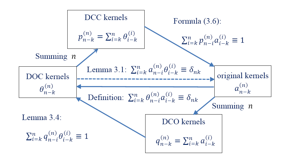
Figure 1: The relationship diagram between different classes of discrete kernels.

Since the kernels $q_{n-j}^{(n)}$ are complementary to the DOC kernels $\theta_{n-j}^{(n)},$ we call $q_{n-j}^{(n)}$ as the discrete complementary-to-orthogonal (DCO) kernels. This terminology is used to distinguish it from the discrete complementary convolution (DCC) kernels $p_{n-j}^{(n)}$ which are complementary to the original discrete kernels $a_{n-j}^{(n)}$, i.e.,

$$\sum_{j=k}^{n}p_{n-j}^{(n)}a_{j-k}^{(j)}\equiv 1\quad\text{for $1\leq k\leq n$.}$$ (3.6)

We present in Figure 1 the relationships between the mentioned discrete convolution kernels. We notice that the DCC kernels $p_{n-j}^{(n)}$ were originally introduced in [10, 11] for analyzing the direct approximations of Caputo derivative. Here, we shall use the newly introduced DCO kernels $q_{n-j}^{(n)}$ to analyze the direct approximations of the Riemann-Liouville derivative (1.11).

3.2 An equivalent formula and unique solvability

We now derive an equivalent formula for our scheme (2.9)-(2.10). By using the definition (2.2) of L1_R formula, we can write the equation (2.9) as

$$\triangledown_{\!\tau}u^{j}=\tau_{j}({}^{R}\!\partial_{\tau}^{1-\alpha}v)^{j-\frac{1}{2}}=\sum_{k=1}^{j}a_{j-k}^{(j)}v^{k-\frac{1}{2}}\quad\text{for $1\leq j\leq N$.}$$

Multiplying both sides of the above equation by the DOC kernels $\theta_{n-j}^{(n)}$, and summing $j$ from $j=1$ to $n$, we obtain

$$\sum_{j=1}^{n}\theta_{n-j}^{(n)}\triangledown_{\!\tau}u^{j}= \,\sum_{j=1}^{n}\theta_{n-j}^{(n)}\sum_{k=1}^{j}a_{j-k}^{(j)}v^{k-\frac{1}{2}}=\sum_{k=1}^{n}v^{k-\frac{1}{2}}\sum_{j=k}^{n}\theta_{n-j}^{(n)}a_{j-k}^{(j)}$$

$$= \,\sum_{k=1}^{n}v^{k-\frac{1}{2}}\delta_{nk}=v^{n-\frac{1}{2}}\quad\text{for $1\leq n\leq N$,}$$

where the summation order was exchanged in the second equality and the discrete orthogonal identity (3.1) was used in the third equality. Then the equation (2.10) gives an equivalent form of the Crank-Nicolson scheme

$$\sum_{j=1}^{n}\theta_{n-j}^{(n)}\triangledown_{\!\tau}u^{j}=\varepsilon^{2}D_{h}u^{n-\frac{1}{2}}-H(u^{n},u^{n-1})\quad\text{for $1\leq n\leq N$},$$ (3.7)

where the vector $H(u^{n},u^{n-1})$ is defined by (2.11).

The formulation (3.7) looks like a direct approximation of the original equation (1.1) by approximating the Caputo derivative $\partial_{t}^{\alpha}u$ with

$$(\partial_{t}^{\alpha}u)(t_{n-\frac{1}{2}})\approx\sum_{j=1}^{n}\theta_{n-j}^{(n)}\triangledown_{\!\tau}u^{j}.$$ (3.8)

In this sense, the DOC kernels $\theta_{n-j}^{(n)}$ define a “new” discrete Caputo derivative. According to Lemma 3.3, the corresponding discrete kernels $\theta_{n-j}^{(n)}$ are positive and monotonously decreasing on nonuniform time meshes, as the case of L1 formula [10, 11, 12]. Nonetheless, we view the formula (3.8) as an indirect approximation that admits different approximation accuracy compared to the original L1 formula with the approximation error of $2-\alpha$.

Next, we shall proof the solvability and discrete maximum bound principle via the new form (3.7). To this end, we shall also need the following lemma for which the proof is similar as in [5, Lemma 3.2].

Lemma 3.5.

Let the elements of a real matrix $B=(b_{ij})_{M\times{M}}$ fulfill $b_{ii}=-\max_{i}\sum_{j\neq{i}}|b_{ij}|\,.$ For any parameters $a,c>0$ and $U,V\in{\mathbb{R}^{M}}$, it holds that

$$\big{\|}\left(aI-B\right)V\big{\|}_{\infty}\geq{a}\big{\|}V\big{\|}_{\infty}$$

and

$$\big{\|}\left(aI-B\right)V+U^{.2}\circ V+cV^{.3}\big{\|}_{\infty}\geq{a}\big{\|}V\big{\|}_{\infty}+\big{\|}U\big{\|}_{\infty}^{2}\big{\|}V\big{\|}_{\infty}+c\big{\|}V\big{\|}_{\infty}^{3}.$$

Now we are ready to present the unique solvability of our scheme.

Theorem 3.1.

The nonlinear Crank-Nicolson scheme (3.7) or (2.9)-(2.10) is uniquely solvable if the time-step size satisfies

$$\tau<\sqrt[\alpha]{2\Gamma(1+\alpha)}.$$

Proof.

We rewrite the nonlinear scheme (3.7) into

$$G_{h}u^{n}+\frac{1}{3}(u^{n})^{.3}=\mathrm{G}_{0}(u^{n-1}),\quad{n}\geq{1},$$

where

$$G_{h}:=\Big{(}\theta_{0}^{(n)}-\frac{1}{2}+\frac{1}{2}(u^{n-1})^{.2}\Big{)}I-\frac{\varepsilon^{2}}{2}D_{h}$$

and

$$\mathrm{G}_{0}(u^{n-1}):= \,\frac{1}{2}(I+\varepsilon^{2}D_{h})u^{n-1}-\frac{1}{6}(u^{n-1})^{.3}+\sum_{k=1}^{n-1}\big{(}\theta_{n-k-1}^{(n)}-\theta_{n-k}^{(n)}\big{)}u^{k}+\theta_{n-1}^{(n)}u^{0}\quad\text{for $n\geq 1$}.$$

If the maximum step size $\tau<\sqrt[\alpha]{2\Gamma(1+\alpha)}$, Lemma 3.2 shows that

$$\theta_{0}^{(n)}=\Gamma(1+\alpha)\tau_{n}^{-\alpha}>1/2.$$

Then by Lemma 2.2 (b), the symmetric matrix $G_{h}$ is positive definite. Thus, the solution of nonlinear equations solves

$$u^{n}=\arg\min_{w\in\mathbb{V}_{h}}\left\{\frac{1}{2}w^{T}G_{h}w+\frac{1}{12}\sum_{k=1}^{M}w_{k}^{4}-w^{T}\mathrm{G}_{0}(u^{n-1})\right\}\quad\text{for $n\geq 1$.}$$

The strict convexity of objective function implies the unique solvability of (3.7). ∎

3.3 Discrete maximum bound principle

We next show that our scheme admits the discrete maximum bound principle.

Theorem 3.2.

Assume that the time-step size satisfies

$$\tau_{n}\leq\sqrt[\alpha]{\min\Big{\{}\frac{1}{2},\frac{h^{2}}{2\varepsilon^{2}}\Big{\}}\frac{\alpha\,\Gamma(1+\alpha)}{(1+r_{n})^{1-\alpha}}}\,.$$ (3.9)

Then, the Crank-Nicolson scheme (3.7) or (2.9)-(2.10) preserves the maximum bound principle at the discrete levels, that is,

$$\big{\|}u^{k}\big{\|}_{\infty}\leq{1}\;\;\text{for $1\leq{k}\leq{N}$}\quad\text{if}\;\;\big{\|}u^{0}\big{\|}_{\infty}\leq{1}.$$

Proof.

According to Theorem 3.1, the time-step restriction (3.9) ensures the solvability of (3.7) since $(1+r_{n})^{\alpha-1}<1$. Now we consider a mathematical induction proof. Obviously, the claimed inequality holds for $n=0$. For $1\leq n\leq N$, assume that

$$\big{\|}u^{k}\big{\|}_{\infty}\leq{1}\quad\text{for $0\leq{k}\leq{n-1}.$}$$ (3.10)

It remains to verify that $\big{\|}u^{n}\big{\|}_{\infty}\leq{1}$. Note that

$$\sum_{j=1}^{n}\theta_{n-j}^{(n)}\triangledown_{\!\tau}u^{j}=\theta_{0}^{(n)}u^{n}-\big{(}\theta_{0}^{(n)}-\theta_{1}^{(n)}\big{)}u^{n-1}-\mathcal{L}^{n-2}(u),$$

where $\mathcal{L}^{n-2}(u)$ is given by

$$\mathcal{L}^{n-2}(u):=\sum_{k=1}^{n-2}\big{(}\theta_{n-k-1}^{(n)}-\theta_{n-k}^{(n)}\big{)}u^{k}+\theta_{n-1}^{(n)}u^{0}.$$ (3.11)

Then the scheme (3.7) can be formulated as follows

$$\,\Big{(}\theta^{(n)}_{0}-\frac{1}{2}+\frac{1}{2}(u^{n-1})^{.2}-\frac{\varepsilon^{2}}{2}D_{h}\Big{)}u^{n}+\frac{1}{3}(u^{n})^{.3}$$

$$\,\hskip 56.9055pt=\big{(}\theta_{0}^{(n)}-\theta_{1}^{(n)}\big{)}u^{n-1}+\frac{\varepsilon^{2}}{2}D_{h}u^{n-1}+\frac{1}{2}u^{n-1}-\frac{1}{6}(u^{n-1})^{.3}+\mathcal{L}^{n-2}(u)$$

$$\,\hskip 56.9055pt=\mathbf{M}_{h}u^{n-1}+\frac{1}{6}\left[3u^{n-1}-(u^{n-1})^{.3}\right]+\mathcal{L}^{n-2}(u),$$ (3.12)

where the matrix $\mathbf{M}_{h}$ is defined by

$$\mathbf{M}_{h}:=\big{(}\theta_{0}^{(n)}-\theta_{1}^{(n)}\big{)}I+\frac{\varepsilon^{2}}{2}D_{h}.$$ (3.13)

For the first term of the right hand side of (3.3), it is easy to check that the matrix $\mathbf{M}_{h}=(m_{ij})$ satisfies $m_{ij}\geq 0$ for $i\neq j$,

$$m_{ii}=\theta_{0}^{(n)}-\theta_{1}^{(n)}-\frac{2\varepsilon^{2}}{h^{2}}\quad\text{and}\quad\max_{i}\sum_{j}m_{ij}\leq\theta_{0}^{(n)}-\theta_{1}^{(n)}.$$

Assuming that $\tau_{n}\leq\sqrt[\alpha]{\frac{h^{2}}{2\varepsilon^{2}}\Gamma^{2}(1+\alpha)\omega_{\alpha}(1+r_{n})}$, we apply Lemma 3.2 to find

$$\theta_{0}^{(n)}-\theta_{1}^{(n)}>\Gamma^{2}(1+\alpha)\omega_{\alpha}(1+r_{n})\tau_{n}^{-\alpha}\geq\frac{2\varepsilon^{2}}{h^{2}}$$

or $m_{ii}\geq 0$. Thus all elements of $\mathbf{M}_{h}$ are nonnegative and

$$\big{\|}\mathbf{M}_{h}\big{\|}_{\infty}=\max_{i}\sum_{j}\left|m_{ij}\right|=\max_{i}\sum_{j}m_{ij}\leq\theta_{0}^{(n)}-\theta_{1}^{(n)}.$$ (3.14)

Consequently, the induction hypothesis (3.10) yields

$$\big{\|}\mathbf{M}_{h}u^{n-1}\big{\|}_{\infty}\leq\big{\|}\mathbf{M}_{h}\big{\|}_{\infty}\big{\|}u^{n-1}\big{\|}_{\infty}\leq\frac{1}{2}\big{(}\theta_{0}^{(n)}-\theta_{1}^{(n)}\big{)}\left(1+\big{\|}u^{n-1}\big{\|}_{\infty}\right).$$ (3.15)

Since $\left|3z-z^{3}\right|\leq 2$ for any $z\in[-1,1]$, the induction hypothesis (3.10) yields

$$\frac{1}{6}\big{\|}3u^{n-1}-(u^{n-1})^{.3}\big{\|}_{\infty}\leq\frac{1}{3}.$$ (3.16)

For the last term $\mathcal{L}^{n-2}(u)$ in (3.3), the decreasing property in Lemma 3.3 and the induction hypothesis (3.10) lead to

$$\big{\|}\mathcal{L}^{n-2}(u)\big{\|}_{\infty}\leq\sum_{k=1}^{n-2}\big{(}\theta_{n-k-1}^{(n)}-\theta_{n-k}^{(n)}\big{)}\big{\|}u^{k}\big{\|}_{\infty}+\theta_{n-1}^{(n)}\big{\|}u^{0}\big{\|}_{\infty}\leq\theta_{1}^{(n)}.$$ (3.17)

Moreover, the time-step restriction (3.9) implies $\tau_{n}<\sqrt[\alpha]{\Gamma(1+\alpha)/2}$ and Lemma 3.2 gives $\theta^{(n)}_{0}>2$. Then by using Lemmas 2.2 and 3.5, one can bound the left hand side of (3.3) by

$$\Big{\|}\big{(}\theta^{(n)}_{0}-\frac{1}{2}-\frac{\varepsilon^{2}}{2}D_{h}\big{)}u^{n}+\frac{1}{2}(u^{n-1})^{.2}\circ u^{n}+\frac{1}{3}(u^{n})^{.3}\Big{\|}_{\infty}$$

$$\hskip 105.2751pt\geq\big{(}\theta^{(n)}_{0}-\frac{1}{2}\big{)}\big{\|}u^{n}\big{\|}_{\infty}+\frac{1}{2}\big{\|}u^{n-1}\big{\|}_{\infty}^{2}\big{\|}u^{n}\big{\|}_{\infty}+\frac{1}{3}\big{\|}u^{n}\big{\|}_{\infty}^{3}.$$

Consequently, by collecting the estimates (3.15)–(3.17), it follows from (3.3) that

$$\big{(}\theta^{(n)}_{0}-\frac{1}{2}\big{)} \,\big{\|}u^{n}\big{\|}_{\infty}+\frac{1}{2}\big{\|}u^{n-1}\big{\|}_{\infty}^{2}\big{\|}u^{n}\big{\|}_{\infty}+\frac{1}{3}\big{\|}u^{n}\big{\|}_{\infty}^{3}$$

$$\leq \,\big{\|}\mathbf{M}_{h}u^{n-1}+\frac{1}{2}\big{(}\theta_{0}^{(n)}-\theta_{1}^{(n)}\big{)}u^{n-1}+\frac{1}{6}\big{[}3u^{n-1}-(u^{n-1})^{.3}\big{]}+\mathcal{L}^{n-2}(u)\big{\|}_{\infty}$$

$$\leq \,\big{\|}\mathbf{M}_{h}u^{n-1}\big{\|}_{\infty}+\frac{1}{6}\big{\|}3u^{n-1}-(u^{n-1})^{.3}\big{\|}_{\infty}+\big{\|}\mathcal{L}^{n-2}(u)\big{\|}_{\infty}$$

$$\leq \,\frac{1}{2}\big{(}\theta_{0}^{(n)}-\theta_{1}^{(n)}\big{)}\left(1+\big{\|}u^{n-1}\big{\|}_{\infty}\right)+\frac{1}{3}+\theta_{1}^{(n)}.$$ (3.18)

Assuming that $\tau_{n}\leq\sqrt[\alpha]{\frac{1}{2}\Gamma^{2}(1+\alpha)\omega_{\alpha}(1+r_{n})}$ such that $\theta_{0}^{(n)}-\theta_{1}^{(n)}>2$, we prove $\big{\|}u^{n}\big{\|}_{\infty}\leq 1$ by contradiction. If $\big{\|}u^{n}\big{\|}_{\infty}>1$, the above inequality (3.3) requires

$$\theta^{(n)}_{0}-\frac{1}{2}+\frac{1}{2}\big{\|}u^{n-1}\big{\|}_{\infty}^{2}+\frac{1}{3}<\frac{1}{2}\big{(}\theta_{0}^{(n)}-\theta_{1}^{(n)}\big{)}\left(1+\big{\|}u^{n-1}\big{\|}_{\infty}\right)+\frac{1}{3}+\theta_{1}^{(n)}$$

because the following function

$$g(z):=\big{(}\theta^{(n)}_{0}-\frac{1}{2}+\frac{1}{2}\big{\|}u^{n-1}\big{\|}_{\infty}^{2}\big{)}z+\frac{1}{3}z^{3}\quad\text{for $z>0$}$$

is monotonically increasing. It follows that

$$\frac{1}{2}\left(1-\big{\|}u^{n-1}\big{\|}_{\infty}\right)^{2}<\frac{1}{2}\big{(}\theta_{0}^{(n)}-\theta_{1}^{(n)}-1-\big{\|}u^{n-1}\big{\|}_{\infty}\big{)}\left(1-\big{\|}u^{n-1}\big{\|}_{\infty}\right)<0,$$

which yields a contradiction. Thus, the assumption $\big{\|}u^{n}\big{\|}_{\infty}>1$ is invalid and the claimed result holds for $k=n$. This completes the proof. ∎

Note that, the maximum time-step restriction (3.9) is only a sufficient condition to ensure the discrete maximum principle, see Example 2. In the time-fractional Allen-Cahn equation (1.1), the coefficient $\varepsilon\ll 1$ represents the width of diffusive interface. Always, we should choose a small space length $h=O(\varepsilon)$ to track the moving interface. So, in most situations, the restriction (3.9) is practically reasonable because it is approximately equivalent to

$$\tau_{n}\leq\sqrt[\alpha]{\frac{\alpha\,\Gamma(1+\alpha)}{2(1+r_{n})^{1-\alpha}}}\rightarrow\frac{1}{2}\quad\text{as $\alpha\rightarrow 1$.}$$

As expected, this restriction (3.9) requires small time steps for large step ratios $r_{n}$ or small fractional orders $\alpha$, see similar conditions in [13]. On the other hand, this time-step condition is sharp in the sense that it is compatible with the previous restriction [5, Theorem 1] ensuring the discrete maximum principle of Crank-Nicolson scheme for the classical Allen-Cahn equation.

4 Numerical experiments

In this section, we shall present several numerical examples to support our theoretical findings. To speed up our numerical computations, we shall use the fast L1_R algorithm described in Appendix B, with an absolute tolerance error $\epsilon=10^{-12}$ and a cut-off time $\Delta{t}=10^{-12}$.

4.1 Accuracy verification

We first show the accuracy of our scheme. Notice that it was shown that the L$1_{R}$ formula (2.2) has been investigated in [17, 18] for linear subdiffusion problems, and the approximation order is shown to be $1+\alpha.$ Thus, we also expect a $(1+\alpha)$-order rate of convergence.

Example 1.

Consider the exterior-forced model

$$\partial_{t}u=-{}^{R}\!\partial_{t}^{1-\alpha}\big{(}\frac{\delta E}{\delta u}\big{)}+g(\mathbf{x},t)$$

on the space-time domain $(0,1)^{2}\times(0,1]$ with an interfacial coefficient $\varepsilon=0.1$. We choose a exterior force $g(\mathbf{x},t)$ and a parameter $\sigma\in(0,1)$ such that the model has an exact solution $u=\omega_{1+\sigma}(t)\sin(2\pi x)\sin(2\pi y)$.

Table 1: Time accuracy for $\alpha=0.6,\,\sigma=0.4.$

  $N$ $\tau$ $\gamma=2$ $\tau$ $\gamma=4=\gamma_{\text{opt}}$ $\tau$ $\gamma=5$ $e(N)$ Order $e(N)$ Order $e(N)$ Order 200 1.39e-02 8.33e-03 $-$ 1.76e-02 7.05e-04 $-$ 1.68e-02 3.82e-04 $-$ 400 7.26e-03 4.81e-03 0.84 9.24e-03 2.47e-04 1.63 8.62e-03 1.13e-04 1.83 800 3.66e-03 2.77e-03 0.81 4.33e-03 8.44e-05 1.41 4.54e-03 3.24e-05 1.95 1600 1.94e-03 1.59e-03 0.87 2.15e-03 2.87e-05 1.55 2.20e-03 9.12e-06 1.75 3200 9.19e-04 9.13e-04 0.74 1.10e-03 9.61e-06 1.63 1.13e-03 2.99e-06 1.68 $\min\{1+\alpha,\gamma\sigma\}$ 0.80 1.60 1.60  

Table 2: Time accuracy for $\alpha=0.8,\,\sigma=0.6.$

  $N$ $\tau$ $\gamma=2$ $\tau$ $\gamma=3=\gamma_{\text{opt}}$ $\tau$ $\gamma=4$ $e(N)$ Order $e(N)$ Order $e(N)$ Order 200 1.42e-02 6.97e-04 $-$ 1.58e-02 1.31e-04 $-$ 1.74e-02 6.44e-05 $-$ 400 8.02e-03 3.07e-04 1.44 8.73e-03 4.07e-05 1.97 8.62e-03 1.71e-05 1.88 800 3.73e-03 1.34e-04 1.08 4.13e-03 1.25e-05 1.58 4.46e-03 4.39e-06 2.07 1600 1.93e-03 5.86e-05 1.26 2.07e-03 3.77e-06 1.73 2.10e-03 1.13e-06 1.80 3200 9.53e-04 2.55e-05 1.18 1.06e-03 1.13e-06 1.82 1.13e-03 4.15e-07 1.63 $\min\{1+\alpha,\gamma\sigma\}$ 1.20 1.80 1.80  

To resolve the initial singularity, we split the time interval $[0,T]$ into two parts $[0,T_{0}]$ and $[T_{0},T]$ with total $N$ subintervals. A graded mesh $t_{k}=T_{0}(k/N_{0})^{\gamma}$ is employed with $T_{0}=\min\{1/\gamma,T\}$ and $N_{0}=\lceil\frac{N}{T+1-\gamma^{-1}}\rceil$ in the first part $[0,T_{0}]$. In the remainder interval $[T_{0},T]$, we use random step sizes

$$\tau_{N_{0}+k}:=\frac{(T-T_{0})\epsilon_{k}}{\sum_{k=1}^{N-N_{0}}\epsilon_{k}}\quad\text{for $1\leq k\leq N-N_{0}$,}$$

where $\epsilon_{k}$ are uniformly distributed random numbers inside $(0,1)$.

We focus on the time accuracy of the modified Crank-Nicolson scheme (2.9)-(2.10). Always, the spatial domain $\Omega=(0,1)^{2}$ is uniformly discretized by using $512\times 512$ grids such that the temporal error dominates. We record the maximum norm error $e(N):=\max_{1\leq{n}\leq{N}}\|u(t_{n})-u^{n}\|_{\infty}$ in each run and evaluate the convergence order by

$$\text{Order}\approx\frac{\log\left(e(N)/e(2N)\right)}{\log\left(\tau(N)/\tau(2N)\right)},$$

where $\tau(N)$ denotes the maximum time-step size for total $N$ subintervals. We run the new scheme by considering the following two cases:

1. The fractional order $\alpha=0.6$ and regularity parameter $\sigma=0.4$ with mesh parameters $\gamma=2,4,5$, respectively (see Table 1);

2. The fractional order $\alpha=0.8$ and regularity parameter $\sigma=0.6$ with mesh parameters $\gamma=2,3,4$, respectively (see Table 2).

From Tables 1 and 2, one can observe that an optimal rate $\mathcal{O}\left(\tau^{\{\gamma\sigma,1+\alpha\}}\right)$ is achieved when the grading parameter $\gamma\geq\gamma_{\text{opt}}=\max\{1,(1+\alpha)/\sigma\}$. As noticed, the error analysis in [17, 18] is only suited for the graded meshes. Thus there is still a gap between the numerical evidences and the theoretical verification of convergence rates on a general class of nonuniform time meshes.

4.2 Discrete maximum bound principle

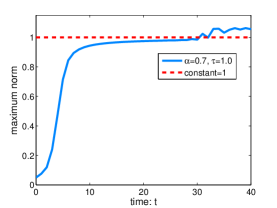
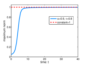
Figure 2: The maximum norm of discrete solutions for the fractional orders $\alpha=0.7,0.9$ (from top to bottom) with three different time-step sizes $\tau=0.1,0.8,1.0$ (from left to right).

We now verify the discrete maximum bound principle. For the fractional orders $\alpha=0.7$ and $0.9$, we run the numerical scheme (2.9)-(2.10) with the random initial data $u_{0}(\mathbf{x})=\mathrm{rand}(\mathbf{x})$ until $T=40$ on different uniform meshes. Figure 2 plots the maximum norm for two fractional order $\alpha=0.7,0.9$ with three different time-step size $\tau=0.1,0.8,1.0$. These results suggest that the time-step restriction (3.9) is only sufficient to ensure the maximum maximum principle. Actually, the step-size restriction (3.9) requires the maximal step size $\tau\leq 0.14$ for the fractional order $\alpha=0.7$ and requires $\tau\leq 0.36$ as the fractional order $\alpha=0.9$.

4.3 Initial singularity and graded meshes

Example 2.

Consider the time-fractional Allen-Cahn equation (1.1) on the physical domain $(0,2\pi)^{2}$ with the model parameter $\varepsilon=0.05$. The initial condition is taken as $u_{0}(\mathbf{x})=\mathrm{rand}(\mathbf{x})$, where $\mathrm{rand}(\mathbf{x})$ is uniformly distributed random number varying from $-0.001$ to $0.001$ to each grid points. Always, a $128\times 128$ uniform spatial mesh is used to cover the domain $(0,2\pi)^{2}$.

Figure 3: The log-log plot of $\partial_{\tau}u^{n-\frac{1}{2}}$ versus time for (1.1) with $\alpha=0.7$ and grading parameters $\gamma=1,\,3$ (from left to right). The legends refer to the spatial positions.

We run the scheme (2.9)-(2.10) with fractional order $\alpha=0.7$, $T=1/\gamma$ and $u_{0}(\mathbf{x})=\mathrm{rand}(\mathbf{x})$. Figure 3 depicts the discrete time derivative $\partial_{\tau}u^{n-\frac{1}{2}}$ near $t=0$ on the graded mesh $t_{n}=T(n/N)^{\gamma}$ for two grading parameters $\gamma=1,3$. It is seen that

$$\log|u_{t}(\mathbf{x},t)|\approx(\alpha-1)\log(t)+C(\mathbf{x})\;\;\text{such that $u_{t}=\mathcal{O}(t^{\alpha-1})$}\quad\text{as $t\rightarrow 0$,}$$

and the initial singularity can be resolved by concentrating more grids near initial time.

4.4 Adaptive time stepping

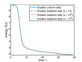
Figure 4: The energies $E(t)$, $E_{\alpha}(t)$ and adaptive steps of Example 2.

Table 3: Comparisons of CPU time (in seconds) and time steps.

  Adaptive parameter $\kappa=10$ $\kappa=10^{2}$ $\kappa=10^{3}$ uniform mesh CPU time 41.167 61.596 136.787 321.830 Time steps 507 769 1734 4000  

In order to resolve the dynamic evolutions involving multiple time scales and reduce the computation cost in long time simulations, we next present an adaptive time-stepping strategy [21] with the following adaptive step criterion based on the energy variation,

$$\tau_{ada}=\max\Bigg{\{}\tau_{\min},\frac{\tau_{\max}}{\sqrt{1+\kappa\left|E_{\alpha}^{\prime}(t)\right|^{2}}}\Bigg{\}},$$

where $E_{\alpha}$ is the modified energy (1.16), $\tau_{\max},\tau_{\min}$ are the predetermined maximum and minimum time steps, respectively. The parameter $\kappa$ is chosen to adjust the level of adaptivity. In our computations, the time interval $[0,T]$ is divided into $[0,T_{0}]$ and $[T_{0},T]$. We choose the graded mesh $t_{k}=T_{0}(k/N_{0})^{\gamma}$ with $T_{0}=0.01$, $N_{0}=30$ and $\gamma=3$ in the starting cell $[0,T_{0}]$. The remainder $[T_{0},T]$ is tested by two types of time meshes:

(Graded-uniform mesh)

Uniform step size $\tau=0.01$;

(Graded-adaptive mesh)

Adaptive time-stepping with $\tau_{\max}=10^{-1}$ and $\tau_{\min}=10^{-3}$.

Figure 5: The energies $E(t)$, $E_{\alpha}(t)$ and adaptive steps of Example 2.

Table 4: Comparisons of CPU time (in seconds) and time steps.

  Adaptive parameter $\kappa=10$ $\kappa=10^{2}$ $\kappa=10^{3}$ uniform mesh CPU time 41.167 61.596 136.787 321.830 Time steps 507 769 1734 4000  

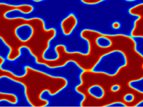
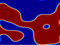
Figure 6: Solution snapshots of Example 2 at $t=10,50,100,300$ (from left to right) for fractional orders $\alpha=0.4,\,0.7$ and $0.9$ (from top to bottom), respectively.

Figure 5 presents the discrete original energy $E(t)$, the discrete modified energy $E_{\alpha}(t)$ and different time steps for simulating Example 2 with $u_{0}(\mathbf{x})=\mathrm{rand}(\mathbf{x})$ until $T=40$. Table 4 lists the CPU time and the corresponding number of time steps for different time-stepping strategies. The two diagrams in Figure 5 show that the original and modified energies computed on the graded-adaptive mesh coincide with those on the graded-uniform mesh. Table 4 indicates that the graded-adaptive time-stepping strategy with appropriate parameter $\kappa$ is computationally more efficient than the graded-uniform mesh. Also, we see that the parameter $\kappa$ affects the level of adaptivity, i.e., the bigger the value of $\kappa$, the smaller the adaptive steps.

Figure 7: Evolutions of energies $E(t)$ , $E_{\alpha}(t)$, maximum norm and adaptive time steps (form left to right) of Example 2 for three fractional orders $\alpha=0.4,\,0.7$ and $0.9$, respectively.

Now we use the graded-adaptive time-stepping strategy with $\kappa=10^{3}$ to simulate the coarsening dynamics of Example 2 until $T=300$. The time evolutions of the microstructure due to phase separation is summarized in Figure 6. The time evolutions of discrete energies, $E(t)$ and $E_{\alpha}(t)$, the discrete maximum principle, and adaptive time steps are displayed in Figure 7. As seen, the coarsening dynamics for a big fractional order $\alpha$ is faster than that for a small one. Correspondingly, the bigger the fractional order $\alpha,$ the faster the original energy $E(t)$ dissipates. Due to the convolution term $\mathcal{I}_{t}^{\alpha}\left\|\frac{\delta E}{\delta u}\right\|^{2},$ the variational energy $E_{\alpha}(t)$ yields a sightly different behavior. The time-step curves show that small time steps are selected during the early separation progress having a large variation of energy; large time-steps are chosen during the coarsening progress having a small variation of energy. Moreover, the time evolution of coarsening dynamics preserves the discrete maximum principle well.

5 Concluding remarks

We proposed a Crank-Nicolson scheme with variable steps for the time fractional Allen-Cahn equation that can preserve both the energy stability and the maximum bound principle. More importantly, the scheme is asymptotically energy stability preserving in the $\alpha\rightarrow 1$ limit. Our scheme is build on a reformulated problem associated with the Riemann-Liouville derivative. In this way, we build up for the first time a reversible discrete transformation between the L1-type formula of Riemann-Liouville derivative and a new L1-type formula of Caputo derivative.

This work raises some open issues to be further studied:

• The numerical rate of convergence of our scheme is $1+\alpha.$ Thus it is worth to design a second order scheme that can preserve both the maximum bound principle and the variational energy dissipation law. One possible way to do this is the recently suggested second-order formula in [20] by replacing the piecewise constant approximation $\Pi_{0}v$ with the piecewise linear polynomial $\Pi_{1}v$ in (2.2).

• By the DOC kernels (3.1), we build a connection between the discrete L1 Riemann-Liouville derivative (2.2) and an indirect discrete Caputo derivative (3.8). How about other discrete Riemann-Liouville derivatives, such as the variable-step second-order approximation in [20]? Lemma 3.1 suggests that there exist (indirect) discrete Riemann-Liouville formulas for any existing numerical Caupto derivatives, including the L1, Alikhanov (L2-1_σ) and L1⁺ formulas, then it would be interesting to investigate numerical approximation properties for those associated discrete Riemann-Liouville approximations.

Appendix A Approximation of the nonlinear bulk

We consider a second-order approximation of the nonlinear bulk force $f(u)=u^{3}-u$. It is easy to check the following equalities

$$4f(a)\left(a-b\right)= \,(1-a^{2})^{2}-(1-b^{2})^{2}-2(1-a^{2})(a-b)^{2}+(a^{2}-b^{2})^{2},$$

$$4f(b)\left(a-b\right)= \,(1-a^{2})^{2}-(1-b^{2})^{2}+2(1-b^{2})(a-b)^{2}-(a^{2}-b^{2})^{2}.$$

Then one can obtain that

$$\frac{1}{2}\left[f(a)+f(b)\right](a-b)=F(a)-F(b)+\frac{1}{4}(a+b)(a-b)^{3}.$$

We consider a function $H(a,b)$ with a real parameter $\nu$,

$$H(a,b):=\frac{1}{2}\left[f(a)+f(b)\right]-\frac{1}{4}\left[(2-\nu)a+\nu b\right](a-b)^{2}$$

such that

$$H(a,b)(a-b)=F(a)-F(b)+\frac{\nu-1}{4}(a-b)^{4}\geq F(a)-F(b)\quad\text{if $\nu\geq 1$.}$$

Moreover, the stabilized term in $H(a,b)$ contains

$$\left[(2-\nu)a+\nu b\right](a-b)^{2}=(2-\nu)a^{3}+(3\nu-4)a^{2}b+(2-3\nu)ab^{2}+\nu b^{3}.$$

One can choose $\nu=4/3$ to eliminate the term $a^{2}b$ so that $H(a,b)$ contains only the terms $a^{3}$, $ab^{2}$ and $b^{3}$. Thus we have

$$H(a,b)=\frac{1}{2}\left[f(a)+f(b)\right]-\frac{1}{6}(a+2b)(a-b)^{2}=\frac{1}{3}a^{3}+\frac{1}{2}ab^{2}+\frac{1}{6}b^{3}-\frac{1}{2}(a+b),$$ (A.1)

$$H(a,b)(a-b)=F(a)-F(b)+\frac{1}{12}(a-b)^{4}.$$ (A.2)

The function $H(a,b)$ in (A.1) will present a second-order approximation of the function $f$ over the interval $[a,b]$. Note that, the equality (A.2) is vital to the unconditional energy dissipation of the suggested method, see Theorem 2.1. Furthermore, the following property

$$\frac{\partial H}{\partial a}(a,b)=a^{2}+\frac{1}{2}(b^{2}-1)$$ (A.3)

is important to the unique solvability and maximum bound principle of our nonlinear scheme, see Theorem 3.1 and Theorem 3.2.

Appendix B Fast computations of L1_R formula

Always, the L1_R fromula (2.2) needs huge storage and computational cost in long time simulations due to the non-locality of Riemann-Liouville derivative (1.11). To reduce the computational cost and memory requirements, the sum-of-exponentials technique [7, Theorem 2.1] is applied here to speed up the evaluation of the L1_R formula. A key result is to approximate the kernel function $\omega_{\alpha}(t)$ efficiently inside the interval $[\Delta{t},\,T]$.

Lemma B.1.

For the given $\alpha\in(0,\,1)$, an absolute tolerance error $\epsilon\ll{1}$, a cut-off time $\Delta{t}>0$ and a finial time $T$, there exists a positive integer $N_{q}$, positive quadrature nodes $\theta^{\ell}$ and corresponding positive weights $\varpi^{\ell}\,(1\leq{\ell}\leq{N_{q}})$ such that

$$\bigg{|}\omega_{\alpha}(t)-\sum_{\ell=1}^{N_{q}}\varpi^{\ell}e^{-\theta^{\ell}t}\bigg{|}\leq\epsilon,\quad\forall\,{t}\in[\Delta{t},\,T],$$

where the number $N_{q}$ of quadrature nodes satisfies

$$N_{q}=\mathcal{O}\left(\log\frac{1}{\epsilon}\Big{(}\log\log\frac{1}{\epsilon}+\log\frac{T}{\Delta t}\Big{)}+\log\frac{1}{\Delta t}\Big{(}\log\log\frac{1}{\epsilon}+\log\frac{1}{\Delta t}\Big{)}\right).$$

The Riemann-Liouville derivative (1.11) is first split into a local part $[t_{n-1},\,t]$ and a history part $[0,\,t_{n-1}]$. The local part is approximated by the constant interpolation $\left(\Pi_{0,n}v\right)(t)$ and the history part is evaluated via the SOE technique, that is,

$$\left({}^{R}\!\partial_{t}^{\alpha}v\right)(t_{n-\frac{1}{2}}) \approx\frac{1}{\tau_{n}}\int_{t_{n-1}}^{t_{n}}\frac{\partial}{\partial t}\int_{t_{n-1}}^{t}\omega_{\alpha}(t-s)(\Pi_{0,n}v)(s)\,\mathrm{d}{s}\,\mathrm{d}{t}$$

$$\quad+\frac{1}{\tau_{n}}\int_{t_{n-1}}^{t_{n}}\frac{\partial}{\partial t}\int_{0}^{t_{n-1}}v(s)\sum_{\ell=1}^{N_{q}}\varpi^{\ell}e^{-\theta^{\ell}(t-s)}\,\mathrm{d}{s}\,\mathrm{d}{t}$$

$$=\frac{a_{0}^{(n)}}{\tau_{n}}v^{n-\frac{1}{2}}+\frac{1}{\tau_{n}}\sum_{\ell=1}^{N_{q}}\varpi^{\ell}\int_{t_{n-1}}^{t_{n}}\frac{\partial}{\partial t}\int_{0}^{t_{n-1}}v(s)e^{-\theta^{\ell}(t-s)}\,\mathrm{d}{s}\,\mathrm{d}{t}$$

$$=\frac{a_{0}^{(n)}}{\tau_{n}}v^{n-\frac{1}{2}}-\frac{1}{\tau_{n}}\sum_{\ell=1}^{N_{q}}\varpi^{\ell}\big{(}1-e^{-\theta^{\ell}\tau_{n}}\big{)}\mathcal{H}^{\ell}(t_{n-1})\quad\text{for $n\geq 1$,}$$ (B.1)

in which $\mathcal{H}^{\ell}(t_{k})$ is given by

$$\mathcal{H}^{\ell}(t_{k}):=\int_{0}^{t_{k}}e^{-\theta^{\ell}(t_{k}-s)}v(s)\,\mathrm{d}{s}\quad\text{with}\quad\mathcal{H}^{\ell}(t_{0})=0.$$

Applying the constant interpolation $\Pi_{0,k}v$ to approximate $v$ in interval $[t_{k-1},t_{k}]$, one can find the following recursive formula to update $\mathcal{H}^{\ell}(t_{k})$,

$$\mathcal{H}^{\ell}(t_{k}) \approx\int_{0}^{t_{k-1}}e^{-\theta^{\ell}(t_{k}-s)}v(s)\,\mathrm{d}{s}+\int_{t_{k-1}}^{t_{k}}e^{-\theta^{\ell}(t_{k}-s)}v^{k-\frac{1}{2}}\,\mathrm{d}{s}$$

$$=e^{-\theta^{\ell}\tau_{k}}\mathcal{H}^{\ell}(t_{k-1})+v^{k-\frac{1}{2}}\int_{t_{k-1}}^{t_{k}}e^{-\theta^{\ell}(t_{k}-s)}\,\mathrm{d}{s}.$$ (B.2)

Then the two approximations (B)-(B) gives a fast L1_R formula,

$$({}^{R}\!\partial_{f}^{\alpha}v)^{n-\frac{1}{2}}:=\frac{1}{\tau_{n}}a_{0}^{(n)}v^{n-\frac{1}{2}}-\frac{1}{\tau_{n}}\sum_{\ell=1}^{N_{q}}\varpi^{\ell}\big{(}1-e^{-\theta^{\ell}\tau_{n}}\big{)}H^{\ell}(t_{n-1}),$$ (B.3)

where the history $\mathcal{H}^{\ell}(t_{k})$ will be updated by $H^{\ell}(t_{0})=0$ and

$$H^{\ell}(t_{k})=e^{-\theta^{\ell}\tau_{k}}H^{\ell}(t_{k-1})+v^{k-\frac{1}{2}}\int_{t_{k-1}}^{t_{k}}e^{-\theta^{\ell}(t_{k}-s)}\,\mathrm{d}{s}\quad\text{for $k\geq 1$.}$$

References

- [1] S. M. Allen and J. W. Cahn, A microscopic theory for antiphase boundary motion and its application to antiphase domain coarsening, Acta Metall, 27:1085–1095, 1979.
- [2] A. Alsaedi, B. Ahmad and M. Kirane, Maximum principle for certain generalized time and space-fractional diffusion equations, Quart. Appl. Math., 73 (2015), pp. 163-175.
- [3] Q. Du, J. Yang and Z. Zhou, Time-fractional Allen-Cahn equations: analysis and numerical methods, arXiv:1906.06584v1, 2019.
- [4] H. Gomez and T. J. Hughes, Provably unconditionally stable, second-order time-accurate, mixed variational methods for phase-field models, J. Comput. Phys., 230:5310–5327, 2011.
- [5] T. Hou, T. Tang and J. Yang, Numerical analysis of fully discretized Crank-Nicolson scheme for fractional-in-space Allen-Cahn equations, J. Sci. Comput., 72 (2017), pp. 1–18.
- [6] M. Inc, A. Yusuf, A. Aliyu and D. Baleanu, Time-fractional Allen-Cahn and time-fractional Klein-Gordon equations: Lie symmetry analysis, explicit solutions and convergence analysis, Physica A Stat. Mech. Appl., 493:94–106, 2018.
- [7] S. Jiang , J. Zhang, Z. Qian and Z. Zhang. Fast evaluation of the Caputo fractional derivative, its applications to fractional diffusion equations. Comm. Comput. Phys., 21:650–678, 2017.
- [8] B. Ji, H.-L. Liao and L. Zhang, Simple maximum-principle preserving time-stepping methods for time-fractional Allen-Cahn equation, Adv. Comput. Math., 46(2), 2020, doi: 10.1007/s10444-020-09782-2.
- [9] Z. Li, H. Wang and D. Yang, A space-time fractional phase-field model with tunable sharpness and decay behavior and its efficient numerical simulation, J. Comput. Phys., 347:20–38, 2017.
- [10] H.-L. Liao, D. Li and J. Zhang, Sharp error estimate of nonuniform L1 formula for linear reaction-subdiffusion equations, SIAM J. Numer. Anal., 56(2): 1112-1133, 2018.
- [11] H.-L. Liao, W. McLean and J. Zhang, A discrete Grönwall inequality with application to numerical schemes for subdiffusion problems, SIAM J. Numer. Anal., 57(1):218-237, 2019.
- [12] H.-L. Liao, Y. Yan and J. Zhang, Unconditional convergence of a two-level linearized fast algorithm for semilinear subdiffusion equations, J. Sci. Comput., 80(1):1-25, 2019.
- [13] H.-L. Liao, T. Tang and T. Zhou, A second-order and nonuniform time-stepping maximum-principle preserving scheme for time-fractional Allen-Cahn equations, J. Comput. Phys., 414, 2020, 109473.
- [14] H.-L. Liao, T. Tang and T. Zhou, Positive definiteness of real quadratic forms resulting from variable-step approximations of convolution operators, arXiv:2011.13383v1, 2020, submitted.
- [15] H.-L. Liao and Z. Zhang, Analysis of adaptive BDF2 scheme for diffusion equations, Math. Comp., 2019, DOI: 10.1090/mcom/3585.
- [16] H. Liu, A. Cheng, H. Wang and J. Zhao, Time-fractional Allen-Cahn and Cahn-Hilliard phase-field models and their numerical investigation, Comp. Math. Appl., 76:1876–1892, 2018.
- [17] K. Mustapha, An implicit finite difference time-stepping method for a subdiffusion equation with spatial discretization by finite elements, IMA J. Numer. Anal., 31 (2011), 719-739.
- [18] K. Mustapha and J. AlMutawa, A finite difference method for an anomalous subdiffusion equation: theory and applications, Numer. Algor., 61 (2012), 525-543.
- [19] K. Mustapha and W. McLean, Piecewise-linear, discontinuous Galerkin method for a fractional diffusion equation, Numer. Algor., 56 (2011), 159-184.
- [20] K. Mustapha, An L1 approximation for a fractional reaction-diffusion equation, a second-order error analysis over time-graded meshes, SIAM J. Numer. Anal., 58 (2020), 1319–1338.
- [21] Z. Qiao, Z. Zhang and T. Tang, An adaptive time-stepping strategy for the molecular beam epitaxy models, SIAM J. Sci. Comput., 33:1395-1414, 2011.
- [22] C. Quan, T. Tang and J. Yang, How to define dissipation-preserving energy for time-fractional phase-field equations, CSIAM Trans. Appl. Math., 1 (2020), pp. 478-490.
- [23] T. Tang, H. Yu and T. Zhou, On energy dissipation theory and numerical stability for time-fractional phase field equations, SIAM J. Sci. Comput., 41-6 (2019), pp. A3757-A3778.
- [24] J. Zhao, L. Chen, and H. Wang, On power law scaling dynamics for time-fractional phase field models during coarsening, Comm. Non. Sci. Numer. Simu., 70:257–270, 2019.