Minimax Strikes Back

Abstract

Deep Reinforcement Learning (DRL) reaches a superhuman level of play in many complete information games. The state of the art search algorithm used in combination with DRL is Monte Carlo Tree Search (MCTS). We take another approach to DRL using a Minimax algorithm instead of MCTS and learning only the evaluation of states, not the policy. We show that for multiple games it is competitive with the state of the art DRL for the learning performances and for the confrontations.

1 Introduction

Monte Carlo Tree Search (MCTS) (Coulom 2006; Kocsis and Szepesvári 2006; Browne et al. 2012) and its refinements (Cazenave 2015, 2016; Silver et al. 2016) are the current state of the art in complete information games search algorithms. Historically, at the root of MCTS were random and noisy playouts. Many such playouts were necessary to accurately evaluate a state. Since AlphaGo (Silver et al. 2016) and Alpha Zero (Silver et al. 2018) it is not the case anymore. Strong policies and evaluations are now provided by neural networks that are trained with Reinforcement Learning. In AlphaGo and its descendants the policy is used as a prior in the PUCT bandit to explore first the most promising moves advised by the neural network policy and the evaluations replace the playouts. In this paper we advocate that when strong evaluation functions, as those provided by self trained neural networks, are available, MCTS might not be the best algorithm anymore. Minimax algorithms are serious challengers when equipped with a strong evaluation function. In this article, we make a comparison between MCTS and a variant of Minimax, called Unbounded Minimax, which had never been done before. We also compare a recent Minimax-based reinforcement learning framework with the state of the art of reinforcement learning, which also had not been done before.

The remainder of the paper is organized as follows. The second section deals with related work. The third section details search algorithms for complete information games and some of their optimizations. The fourth section presents the two zero learning algorithms we use in this paper and compares them. Section 5 details technical characteristics of the experiments, such as the representation of particular neural networks and the used computing resources. Section 6 experimentally compares the two learning algorithms. Section 7 experimentally compares different search algorithms.

2 Related Work

MCTS has its roots in computer Go (Coulom 2006). It was theoretically defined with the UCT algorithm (Kocsis and Szepesvári 2006) that converges to the Nash equilibrium and uses a well defined bandit, Upper Confidence Bounds (UCB), which minimizes the cumulative regret at each node (Auer, Cesa-Bianchi, and Fischer 2002).

Theoretical bandits were soon replaced with empirical bandits which gave better results. First the RAVE algorithm (Gelly and Silver 2011) improved greatly on UCT for the games of Go and Hex (Cazenave and Saffidine 2009). A later refinement is the GRAVE algorithm that improves on RAVE for many different games (Cazenave 2015) and is used by General Game Playing systems such as in Ludii (Browne et al. 2019).

MCTS was combined with neural networks in AlphaGo, surpassing professional level in the game of Go (Silver et al. 2016). The search algorithm used in AlphaGo is PUCT, a bandit that uses the policy given by the neural network to bias the moves to explore. Later AlphaGo was redesigned to learn from zero knowledge, leading to AlphaGo Zero and zero learning (Silver et al. 2017). It was then applied to other games, namely Shogi and Chess, with the Alpha Zero program (Silver et al. 2018).

Many teams have replicated the Alpha Zero approach for Go and for other games: Elf/OpenGo (Tian et al. 2019), Leela Zero (Pascutto 2017), Crazy Zero by Rémi Coulom, KataGo (Wu 2019), Galvanise Zero (Emslie 2019) and Polygames (Cazenave et al. 2020).

As we use Polygames as a sparring partner we will give more details about it. Polygames replicated the Alpha Zero approach and applied it to many games with success. There are multiple innovations in Polygames. It can train neural networks with an architecture independent of the size of the board. To do so it uses a fully convolutional policy, meaning that there is no dense layer between the last convolutional planes and the policy. The value head is also independent of the size of the board since it uses global average pooling before the dense layers connected to the evaluation output neuron. It is much more difficult to train a network for $19\times 19$ Hex or $13\times 13$ Havannah than training it on a smaller size board. Polygames did succeed in these games by scaling its neural networks trained on smaller sizes to the difficult board sizes. It played on the Little Golem game server and beat the best players at these games that were considered too difficult for Zero Learning. Other innovations of Polygames include a pool of neural networks in self play in order to avoid catastrophic forgetting.

The other kinds of algorithms used in computer games are the $\alpha\beta$ family of algorithms. $\alpha\beta$ dominated the field of complete information games until the advent of MCTS in 2006. Still, many current strong Chess programs use $\alpha\beta$.

There has been a lot of research on the optimizations of the $\alpha\beta$ algorithm (Marsland 1987). Many of them deals with move ordering since moves ordering can drastically improve the thinking time of $\alpha\beta$ based programs (Knuth and Moore 1975).

The search algorithm we use to learn and play games is close to Unbounded Best-first Minimax Search (Korf and Chickering 1996). There is very little study on this algorithm and it seems little or not applied in practice, except in the work of (Cohen-Solal 2020). In that work, variants and improvements of Unbounded Minimax are proposed with several complementary techniques of zero learning that do not require the use of policies, but still manage to achieve a high level of play at the game of Hex (size $11$ and $13$). In the context of the experiments of (Cohen-Solal 2020), the proposed approach is the best learning approach not using a policy: in particular, replacing the used variant of Unbounded Minimax, called descent, by Unbounded Minimax, by $\alpha\beta$ or by MCTS (with UCT) gives less good results. A question then arises, can this approach compete with approaches using a policy, and in particular the state of the art based on MCTS with PUCT. In other words, can it generate strong programs on other games than Hex. Moreover, in the experiments of that work, another variant of Unbounded Minimax, called Unbounded Minimax with Safe decision, is shown best than the Unbounded Minimax or $\alpha\beta$ for the confrontations (“What is the best search algorithm for winning a game ?” is a different question of “What is the best search algorithm to learn faster ?”). However, this comparison is not done with MCTS and with using strong networks. We answer these open questions in this article.

3 Search Algorithms

There are many search algorithms for perfect information games. The two standard algorithms are Monte Carlo Tree Search and Minimax with alpha-beta pruning. We present in this section some of their improvements, used in our experiments.

3.1 Iterative Deepening $\alpha\beta$ with Move Ordering

Iterative deepening $\alpha\beta$ (Fink 1982), denoted $\mathrm{ID}$, is a variant of Minimax with a maximum thinking time. As long as there is time left, the search depth is increased by one and a new search using standard $\alpha\beta$ is performed. In order to make the previous searches profitable, the best move of each state of the previous search is memorized and is played as the first move to explore in the next search. This generally decreases the time for subsequent searches.

3.2 Unbounded Minimax and Safe Unbounded Minimax

The Unbounded (Best-First) Minimax, denoted $\mathrm{UBFM}$, is a variant of Minimax which explores the game tree in a non-homogeneous way. It iteratively extends the best sequence of actions in the game tree (i.e. it adds at each iteration the leafs of the principal variation in the game tree). Therefore, the exploration of the game tree is non-uniform. The best action sequence generally changes after each extension. In general, the worse the evaluation function is, the wider the exploration is. Unbounded Minimax is formally described in Algorithm 1.

The variant of Unbounded Minimax, named Unbounded Best-First Minimax with Safe decision, denoted by $\mathrm{UBFM}_{s}$ (Cohen-Solal 2020) performs the same search as the Unbounded Minimax (i.e. it builds the same partial game tree). The difference is in the decision criteria of the action to be played, after having extended the game tree. To decide which action to play, instead of choosing the best action (i.e. the best minimax value action), it chooses the action that has been selected the most times during the search. It is the safest action in the sense that the number of times an action has been selected is the number of times that this action has been judged superior to other actions.

3.3 Batched Minimax Algorithms

$\mathrm{UBFM}$, $\mathrm{UBFM}_{s}$, and $\mathrm{ID}$ have a natural parallelization with regard to the evaluation of states. It consists of evaluating the leaves of a node in parallel (by batching them in order to evaluate them simultaneously by the neural network). For example, for $\mathrm{UBFM}$, the states $a(s)$ of the foreach block of Algorithm 1 are batched for evaluation. The batched states are thus evaluated by only one (neural) evaluation (which can be executed in parallel on several CPUs or on a GPU). To differentiate the use of this parallelization technique from its non-use, we refer to this improvement as the batched version of the corresponding algorithm.

Function unbounded_minimax_iteration($s$)

      

      if terminal($s$) then

            return $f(s)$

      else

            

            if $s\notin T$ then

                  

                  $T\leftarrow T\cup\{s\}$

                  

                  foreach $a\in$ actions($s$) do

                        $v(s,a)\leftarrow f\left(a(s)\right)$

                        

            else

                  

                  $a_{b}\leftarrow$ best_action($s$)

                  

                  $v(s,a_{b})\leftarrow$ unbounded_minimax_iteration($a_{b}(s)$)

                  

            $a_{b}\leftarrow$ best_action($s$)

            

            return $v(s,a_{b})$

            

Function best_action($s$)

      

      if first_player($s$) then

            return ${\displaystyle\operatorname*{\mathrm{arg\,max}}_{a\in\textnormal{{actions(}}\textnormal{\emph{s}}\textnormal{{)}}}v\left(s,a\right)}$

      else

            return ${\displaystyle\operatorname*{\mathrm{arg\,min}}_{a\in\textnormal{{actions(}}\textnormal{\emph{s}}\textnormal{{)}}}v\left(s,a\right)}$

Function unbounded_minimax($s$, $\tau$)

      

      $t=$ time()

      

      while time()$-\,t<\tau$ do unbounded_minimax_iteration($s$)

      

      return best_action($s$)

      

Algorithm 1 Unbounded Minimax algorithm : it computes the best action to play in the generated non-uniform partial game tree ($a(s)$ : state obtained after playing the action $a$ in the state $s$ ; $v(s,a)$ : value obtained after playing $a$ in $s$ ; $f$ is the used evaluation function ; $T$ : keys of the transposition table (global variable) ; $\tau$ : search time per action).

3.4 First Play Urgency

First-play urgency (FPU) (Wang and Gelly 2007) is an improvement of MCTS. With the standard version of MCTS, there is too much exploration in the states that have been little visited (all the children of a state must be explored before the UCT formula can be used to manage the exploration-exploitation dilemma). FPU adapts the UCT formula so that it is applicable even if some children have not been explored at least once. With FPU, the exploration-exploitation dilemma is managed from the start. So, as soon as one of the explored children is very interesting (“urgent”), it is selected again (even if some children have not been explored at least once).

3.5 Batched MCTS

MCTS virtual loss (Chaslot, Winands, and van Den Herik 2008; Tian et al. 2019) is a multithread technique of MCTS. We use it in some experiments of this article (virtual loss constant is $1$) with rollouts played sequentially and states evaluated in batches of length $b$ after each subsequence of $b$ rollouts (states are thus evaluated in parallel). In this paper, this particular case of MCTS virtual loss is called Batched $\mathrm{MCTS}$.

3.6 Polygames Search Algorithms

Polygames search is based on MCTS with PUCT and First Play Urgency. In some experiments of this article, we use a variant of Polygames which we call Polygames with UCT, a minor modification of the Polygames code, which amounts to using UCT instead of PUCT with First Play Urgency. We also test our program against the original Polygames with heavily trained networks which won computer games competitions.

4 Deep Reinforcement Learning Algorithm

We present in this section the two zero learning frameworks used in the experiments of this article.

4.1 Polygames Learning Algorithm

Polygames uses its search algorithm, MCTS with PUCT and First Play Urgency, to generate games, by playing against itself. It uses the information from these games to update its neural network, which is used by its search algorithm to evaluate states by a value and by a policy (i.e. a probability distribution on the actions to be played in a state). For each finished game, the network is trained to associate with each state of the state sequence the result of the end of that game (which is -1 or 0 or + 1). It is also trained, at the same time, to associate with each state a particular policy whose probability of each action is calculated from the number of time this action is selected in the search from that state.

4.2 Descent Standard Learning Algorithm

The learning framework of (Cohen-Solal 2020) is based on a variant of Unbounded Minimax called descent, dedicated to learning, which consists in playing the sequences of actions until terminal states. The exploration is thus deeper while remaining a best-first approach. This allows the values of terminal states to be propagated more quickly to (shallower) non-terminal states. Unlike Polygames, the learned value of a state is not the end-game value but the minimax value in the partial game tree built during the game. This information is more informative, since it contains part of the knowledge acquired during the previous games. In addition, contrary to Polygames, learning is carried out for each state of the partial game tree constructed during the game (not just for the sequences of states of the played games). As a result, there is no loss of information: all of the information acquired during the search is used during the learning process. An additional advantage is that it generates a much larger amount of data for training. Thus, unlike the state of the art which requires to generate games in parallel to build its learning dataset, this approach does not require the parallelization of games (and this parallelization is not done in the experiments in this article). Finally, this approach is optionally based on a reinforcement heuristic, that is to say an evaluation function of terminal states more expressive than the classical gain of a game (i.e. $+1$ / $0$ / $-1$). The best proposed heuristics in (Cohen-Solal 2020) are scoring and the depth heuristic (the latter favoring quick wins and slow defeats).

Note that this approach does not use a policy, so there is no need to encode actions. Consequently, this avoids the learning performance problem of neural networks for games with large number of actions (i.e. very large output size).

5 Technical Details

In this section, we present neural networks used in some of the experiments of this article and the used computational resources.

5.1 Neural Networks and Parameters for Descent

We use two sets of learning parameters for the descent framework in the experiments of this article. The set of parameters, that we call A-parameters, is: search time per action $\tau=1s$, batch size $B=3000$, memory size $\mu=2\cdot 10^{6}$, sampling rate $\sigma=5\%$ (for more details on these parameters, see Section $3$ of (Cohen-Solal 2020)). The set of parameters, that we call B-parameters, is $\tau=2s$, $B=3000$, $\mu=250$, and $\sigma=2\%$. Moreover, B-parameters includes the use of the data symmetry augmentation, the modified experience replay, and the board sides encoding (see Section 7.2.1 of (Cohen-Solal 2020)).

We use several networks trained by the descent framework. There are $3$ neural networks for the game of Hex, denoted respectively $h_{1}$, $h_{2}$, and $h_{3}$. The values of the $3$ Hex neural networks are in $[-121;121]$ (by using the depth heuristic, terminal states are evaluated based on the duration of games, which lasts, in the case of Hex $11$, at most $121$ turns). The associated learning parameters are the B-parameters, with the following modifications for $h_{1}$ and $h_{2}$: experience replay is not used, $\tau=1s$, and $B=2048$.

Moreover, we respectively use a neural network from the descent framework, training during $30$ days, at the following games: Breakthrough, Othello $8$, and Othello $10$. The learning parameters are the A-parameters. At Othello $8$ and $10$ the scoring heuristic is used, at Breakthrough the depth heuristic is used. The values of the Breakthrough (resp. Othello $8$ ; resp. Othello $10$) neural network is in $[-481;481]$ (resp. $[-64;64]$ ; resp. $[-100;100]$). All descent networks are pre-initialized by the values of random terminal states (around $10^{7}$, i.e. a supervised learning is performed for terminal states from random games. The neural network architectures used in this article are described in Table 2.

layer $\#$	$C$-network	$R_{1}$-network	$R_{2}$-network
$1$	conv. + ReLU	convolution	convolution
$\cdots$	conv. + ReLU	$2$ res. blocks	$8$ res. blocks
$N-2$	conv. + ReLU	$1\times 1$ conv.	dense + ReLU
$N-1$	dense + ReLU	dense + ReLU	dense + ReLU
$N$	dense layer	dense layer	dense layer

Table 1: Description of $3$ neural architectures of value networks, called $C$-network, $R_{1}$-network, and $R_{2}$-network. Each residual block (He et al. 2016) is composed of a ReLU (Glorot, Bordes, and Bengio 2011) followed by a convolution (LeCun, Bengio, and Hinton 2015) followed by a ReLU followed by a convolution followed by a ReLU. Output contains one neuron. Other parameters are: kernel is $3\times 3$, filter number is $F$, neuron number in dense layers is $D$, padding is same for $R_{i}$-network and valid for $C$-network.

network	architecture	$F$	$D$
$h_{1}$, $h_{2}$	$C$-network	$150$	$81$
$h_{3}$	$R_{1}$-network	$240$	$1024$
Breakthrough	$C$-network	$166$	$751$
Othello $8$	$R_{2}$-network	$59$	$213$
Othello $10$	$R_{2}$-network	$59$	$128$

Table 2: Description of the used value neural network architectures in this paper ($F$ and $D$ are parameters of the architecture ; see Table 1).

5.2 Polygames Neural Networks

In the experiments of Section 7.4, we use particular Polygames neural networks which have participated in the TCGA tournament of 2020 (in Taiwan): the Breakthrough network won the tournament, the Othello size $8$ network finished second, and the Othello size $10$ network won the tournament. Their training required the use of 100 to 300 GPU and 80 CPU during 5 to 7 days.

5.3 Computational Resources

For the performed trainings, we use the following hardware: GPU Nvidia Tesla V100 SXM2 32 Go, $2$ to $10$ CPU (processors Intel Cascade Lake 6248 2.5GHz) on RedHat. For the performed confrontations, we use the following hardware: GeForce GTX 1080 Ti, $2$ to $8$ CPU (Intel(R) Xeon(R) CPU E5-2603 v3 1.60GHz) on Ubuntu 18.04.5 LTS.

Descent programs (descent learning, $\mathrm{UBFM}$, $\mathrm{UBFM}_{s}$, $\mathrm{ID}$, $\mathrm{MCTS}$) are coded in Python (using tensorflow 1.12). Polygames is coded in C/C++. For confrontations, Polygames num_actor parameter is $8$ (threads doing MCTS).

6 Comparison of Deep Reinforcement Learning Algorithms

6.1 Game of Hex

In this section, we compare the learning performances of the descent framework (see Section 4.2) with the learning performances of Polygames (see Section 4.1). Several trainings have been carried out on the game Hex (size 11). The descent framework was used to train a first neural network, by using the B-parameters, the depth heuristic, and the C-network architecture (see Sections 4.2 and 5.1). A second network was trained with the same parameters except that the use of the depth heuristic was replaced by the classic gain of a game ($-1$ / $+1$). These two learning processes used between $1$ and $2$ CPU and one GPU (4 trainings were launched in parallel on the same GPU, resulting in a performance loss between $80\%$ and $90\%$). A training was performed with Polygames using a similar network architecture (adapted to have a policy and to keep the same total number of neurons: there are $40$ filters, $50$ dense neurons, the policy is densely connected to the last intermediate layer). Another training was carried out with Polygames using an alphazero-like network architecture with a similar number of neurons ($8$ residual blocks with $64$ filters and $256$ neurons in the dense layers). Each training with Polygames used one GPU and 10 CPUs. The parameters of Polygames training are the default parameters except that num_game=$121$ and act_batchsize=$121$ (they are increased to improve the parallelism). Unlike the training of the two descent networks, the training of the polygames networks does not use the data augmentation symmetry nor the sides encoding. For this reason, a third learning using the descent framework was performed without using these two techniques (by using the A-parameters). The depth heuristic is also not used.

Each training lasted 30 days. In the context of these experiments, the Polygames program has performed $3$ times more state evaluations than the descent program. Each neural network is then evaluated against Mohex 2.0 (Huang et al. 2013), champion program at Hex from 2013 to 2017 at the Computer Olympiads. The search algorithm used to evaluate the descent networks is $\mathrm{UBFM}_{s}$. The Polygames program is used to make the trained Polygames networks play. The evolution of the win percentages against Mohex 2.0 for each program during the learning process is shown in Figure 1. In this experiment, learning with descent is very significantly better than with Polygames. The performance gain is even more marked at the start of learning.

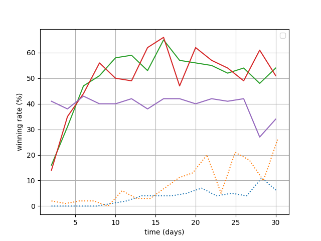
Figure 1: Evolution of winning percentages of descent with classic gain, symmetry and sides encoding (green line), descent with depth heuristic, symmetry and sides encoding (red line), descent with classic gain (purple line), Polygames (orange dotted line), and Polygames using a alphazero neural architecture (blue dotted line) against Mohex 2.0, during a 30 days learning process (approximately one evaluation every two days which consists of 300 matches in first player and 300 other matches in second player).

6.2 Othello $8$ and Breakthrough

A comparison analogous to the previous section was made on Othello $8$ and Breakthrough for a training duration of 6 days. The training using the descent framework on Othello $8$ and Breakthrough is the one described in Section 5.1 (the first 6 days of the 30 days of training). Note: neither symmetry nor sides coding is used.

A GPU and two CPUs have been allocated for each training. The parameters of Polygames training are the default parameters except that num_game=$64$ and act_batchsize=$64$ for Othello $8$, that num_game=$48$ and act_batchsize=$48$ for Breakthrough, and that saving_period=$20$, replay_capacity=$20000$, and replay_warmup=$1000$ (these last parameters have been lowered because the learning time and the number of CPUs are smaller than in the previous section). The used networks with Polygames have a network architecture similar to that of the corresponding descent network (adapted to have a policy and to keep the same number of neurons: the last residual layer is also connected to a dense layer followed by a ReLU, another dense layer, another ReLU, and finally the policy, and there are $32$ (resp. $30$) filters per convolution and $60$ neurons per dense layer for Othello $8$ (resp. for Breakthrough).

At Breakthrough and Othello $8$, the Polygames program using the corresponding network at day $6$ confronts $\mathrm{UBFM}_{s}$ with the corresponding descent network at days $1$, $2$, $3$, $4$, $5$, and $6$. For the day $i$, $i\in\{1,\ldots,6\}$, there are $200$ matchs in first player and $200$ matchs in second player. In each case, the win percentage of $\mathrm{UBFM}_{s}$ is $100\%$.

7 Comparison of Search Algorithms

In this section, we compare Unbounded Minimax ($\mathrm{UBFM}$), Safe Unbounded Minimax ($\mathrm{UBFM}_{s}$), Iterative Deepening Alpha-beta ($\mathrm{ID}$), and Monte Carlo Tree Search ($\mathrm{MCTS}$) between them (in this section $\mathrm{MCTS}$ uses UCT and a value function to evaluate the leaves nodes, except in the subsection 7.4 where it uses PUCT, a value function and also a policy: the standard Polygames program is used).

7.1 Comparison on CPU without batching

We start by comparing them without using a GPU (in their non-batched version). $\mathrm{UBFM}_{s}$, $\mathrm{UBFM}$, Iterative Deepening Alpha-beta and MCTS (for $c\in\{0,\ldots,15$) have been evaluated (on CPU with one processor) against Mohex 2.0 (with four processors) using the neural networks $h_{1}$, $h_{2}$, and $h_{3}$ (see Section 5). The win percentages of these different algorithms are described in Table 3 and Table 4 (only for $c\in\{0,\ldots,5\}$). It is $\mathrm{UBFM}_{s}$ which gets the best win percentages (followed by $\mathrm{UBFM}$) with $1.5s$ and $10s$. Note that the win percentage of MCTS decreases as $c$ increases, which could suggest that in the context of UCT with reinforcement learning (i.e. without policy), there is no point in exploring after the learning process.

We also compare MCTS with UCT and First Play Urgency for different values of $c$, but the results are worse than without First Play Urgency. In this setting the best algorithm is $\mathrm{UBFM}_{s}$. Using the $h_{2}$ network, it even surpasses Mohex.

	$h_{1}$	$h_{2}$	$h_{3}$
$\mathrm{UBFM}_{s}$	$39\%$	$55\%$	$37\%$
$\mathrm{UBFM}$	$32\%$	$51\%$	$32\%$
$\mathrm{ID}$	$31\%$	$43\%$	$28\%$
$\mathrm{MCTS}_{c=0}$	$34\%$	$46\%$	$25\%$
$\mathrm{MCTS}_{c=1}$	$33\%$	$41\%$	$28\%$
$\mathrm{MCTS}_{c=2}$	$31\%$	$39\%$	$24\%$
$\mathrm{MCTS}_{c=3}$	$24\%$	$40\%$	$25\%$
$\mathrm{MCTS}_{c=4}$	$21\%$	$43\%$	$23\%$
$\mathrm{MCTS}_{c=5}$	$15\%$	$39\%$	$23\%$
$\mathrm{MCTS}_{c=10}$	$9\%$	$26\%$	$18\%$
$\mathrm{MCTS}_{c=20}$	$1\%$	$7\%$	$8\%$
$\mathrm{MCTS}_{c=40}$	$0\%$	$1\%$	$8\%$
$\mathrm{MCTS}_{c=80}$	$1\%$	$2\%$	$9\%$

Table 3: Win percentages over $500$ matches as first player and $500$ matches as second player against Mohex 2.0 for different non-batched search algorithms (search time : $1.5s$) for the $3$ Hex neural networks $h_{1}$, $h_{2}$, and $h_{3}$ (see Sect. 5.1).

	$h_{1}$	$h_{2}$	$h_{3}$
$\mathrm{UBFM}_{s}$	$40\%$	$51\%$	$34\%$
$\mathrm{UBFM}$	$36\%$	$47\%$	$28\%$
$\mathrm{ID}$	$28\%$	$30\%$	$16\%$
$\mathrm{MCTS}_{c=0}$	$28\%$	$37\%$	$25\%$
$\mathrm{MCTS}_{c=1}$	$23\%$	$31\%$	$29\%$
$\mathrm{MCTS}_{c=2}$	$25\%$	$32\%$	$25\%$
$\mathrm{MCTS}_{c=3}$	$23\%$	$33\%$	$26\%$
$\mathrm{MCTS}_{c=4}$	$16\%$	$36\%$	$23\%$
$\mathrm{MCTS}_{c=5}$	$15\%$	$38\%$	$23\%$

Table 4: Win percentages over $250$ matches as first player and $250$ matches as second player against Mohex 2.0 for different non-batched search algorithms (search time : $10s$) for the $3$ Hex neural networks $h_{1}$, $h_{2}$, and $h_{3}$ (see Sect. 5.1).

7.2 Comparison on GPU with batching

$\mathrm{UBFM}_{s}$, $\mathrm{UBFM}$, Iterative Deepening Alpha-beta, and MCTS (for $c=0$ and for batch sizes $b\in\{1,2,3,5,8,11\}$) have been evaluated on GPU in their batched version against Mohex 2.0. The win percentages of these different algorithms are described in Table 5. $\mathrm{UBFM}_{s}$ (resp. $\mathrm{UBFM}$) gets the best win percentage with $h_{3}$ and $h_{1}$ (resp. $h_{2}$). Note that the win percentage of MCTS decreases as the batch size increases. In fact, the win percentage continues to decrease for $b\in\{14,17,20,23,26,29,32\}$ (verified by using $h_{2}$).

	$h_{1}$	$h_{2}$	$h_{3}$
$\mathrm{UBFM}_{s}$	$59\%$	$61\%$	$48\%$
$\mathrm{UBFM}$	$35\%$	$72\%$	$44\%$
$\mathrm{ID}$	$33\%$	$51\%$	$27\%$
$\mathrm{MCTS}_{b=1}$	$26\%$	$49\%$	$33\%$
$\mathrm{MCTS}_{b=2}$	$31\%$	$49\%$	$33\%$
$\mathrm{MCTS}_{b=3}$	$33\%$	$46\%$	$26\%$
$\mathrm{MCTS}_{b=5}$	$28\%$	$43\%$	$18\%$
$\mathrm{MCTS}_{b=8}$	$27\%$	$42\%$	$20\%$
$\mathrm{MCTS}_{b=11}$	$26\%$	$38\%$	$16\%$

Table 5: Winning percentages over $300$ matches as first player and $300$ matches as second player against Mohex 2.0 of different batched search algorithms (search time : $1.5s$) for the $3$ Hex neural networks $h_{1}$, $h_{2}$, and $h_{3}$ on GPU.

This experiment has been repeated (with only $\mathrm{UBFM}_{s}$, $\mathrm{MCTS}$ for $b\in\{1,2,4,6\}$, and $h_{2}$) by limiting the search time only by the execution time of the neural network so as to ignore the impact of the python implementation of the game. The results are similar. The win percentages of these different algorithms are described in Table 6.

	$\mathrm{MCTS}$
$\mathrm{UBFM}_{s}$	$b=1$	${b=2}$	$b=4$	$b=6$
$79\%$	$54\%$	$52\%$	$49\%$	$49\%$

Table 6: Winning percentages over $300$ matches as first player and $300$ matches as second player against Mohex 2.0 of different batched search algorithms (neural network time : $1.5s$) using the neural network $h_{2}$ on GPU.

7.3 Exploration constant on Polygames with UCT

In this section, we investigate about the observation of the previous experiment that the exploration term of UCT has turned out to be harmful with a neural network having learned by reinforcement, i.e. that the best value for $c$ is $0$. We compare different values of $c$ for UCT in the framework of Polygames in order to see if our observation does not depend on the used reinforcement learning method. The win percentages of Polygames using UCT (see Section 3.6) depending on $c$ for Hex are described in Table 7. Again, the best exploration value is $c=0$.

rollouts	$94$	$640$	$1600$
$\mathrm{UCT}_{c=1.0}$	$73\%$	$69\%$	$65\%$
$\mathrm{UCT}_{c=0.5}$	$66\%$	$61\%$	$58\%$
$\mathrm{UCT}_{c=0.1}$	$54\%$	$56\%$	$52\%$

Table 7: Winning percentages of Polygames using UCT with $c=0$ againsts Polygames using UCT with $c\in\{0.1,0.5,1\}$ over $169$ matches as first player and $169$ matches as second player for Hex size $11$ and different rollouts (mean over the $13$ best publicly available polygames neural networks at http://dl.fbaipublicfiles.com/polygames/checkpoints/list.txt).

7.4 Comparison versus Tournaments Polygames Networks with PUCT

In this section, we compare, for Breakthrough, Othello $8$ and $10$, several search algorithms using the descent networks of Section 5.1 by making them confront the Polygames program using the networks of Section 5.2, those having won or finished second in the TCGA 2020 tournament.

We start by comparing $\mathrm{UBFM}_{s}$, $\mathrm{UBFM}$, $\mathrm{ID}$, and $\mathrm{MCTS}$ with different exploration constants with a think time of $1.5$ seconds per action. The results are described in Table 8. The best results are for $\mathrm{UBFM}_{s}$ and it is better than Polygames (very significantly at Othello $8$ and $10$). Note that the best exploration constant $c$ of $\mathrm{MCTS}$ is $0.5$, very close to the performance of $c=0$ and $c=0.5$. Relative to the values of states, it is a very small exploration constant. The experiment was then redone, limiting itself to $\mathrm{UBFM}_{s}$ and with $15$ seconds of thinking time per action. The results are described in Table 9. Polygames is this time better at Breakthrough but still worse at Othello $8$ and $10$. The experiment was then redone, with $5$ seconds of thinking time per action. The results are similar but better for $\mathrm{UBFM}_{s}$ (they are described in Table 9).

This experiment was done again with a thinking time of $1.5$ seconds but using the descent networks of day $5$ of the learning process (i.e. the networks were only trained for $5$ days) instead of day $30$. The results are described in Table 10. Polygames is beaten at Breakthrough and Othello $8$. This last experiment was done again with a thinking time of $5$ seconds. The results are described in Table 10. This time, Polygames is better at Breakthrough but $\mathrm{UBFM}_{s}$ is equivalent at Othello $10$ and even better at Othello $8$. In summary, at least after $5$ days of learning, $\mathrm{UBFM}_{s}$ has a level of the same order as Polygames networks at Breakthrough and Othello $10$, but it is better at Othello $8$. After $30$ days of learning, it has slightly improved at Breakthrough and it is significantly superior at Othello $8$ and $10$. Recall that Polygames networks were trained for $5$ to $7$ days but using $100$ to $300$ GPU, against only a “quarter” of one GPU for $\mathrm{UBFM}_{s}$ networks.

	Breakthrough	Othello $8$		Othello $10$
rate	win	win	draw	win	draw
$\mathrm{UBFM}_{s}$	$66\%$	$97\%$	$2\%$	$98\%$	$1\%$
$\mathrm{UBFM}$	$65\%$	$90\%$	$4\%$	$71\%$	$3\%$
$\mathrm{ID}$	$28\%$	$92\%$	$0\%$	$7\%$	$1\%$
$\mathrm{MCTS}_{c=0}$	$28\%$	$71\%$	$1\%$	$30\%$	$1\%$
$\mathrm{MCTS}_{c=\frac{1}{2}}$	$31\%$	$71\%$	$7\%$	$33\%$	$1\%$
$\mathrm{MCTS}_{c=1}$	$33\%$	$53\%$	$3\%$	$37\%$	$1\%$
$\mathrm{MCTS}_{c=\frac{5}{2}}$	$31\%$	$75\%$	$2\%$	$30\%$	$3\%$
$\mathrm{MCTS}_{c=5}$	$27\%$	$67\%$	$3\%$	$18\%$	$1\%$
$\mathrm{MCTS}_{c=10}$	$22\%$	$54\%$	$3\%$	$16\%$	$1\%$
$\mathrm{MCTS}_{c=20}$	$9\%$	$28\%$	$2\%$	$9\%$	$2\%$
$\mathrm{MCTS}_{c=40}$	$1\%$	$19\%$	$3\%$	$6\%$	$1\%$

Table 8: Results of $300$ matches as first player and $300$ other matches as second player of the descent networks of Section 5.1 (with $30$ days of learning) using different search algorithms (minimax algorithms are batched) with $1.5$ seconds of search time per action at Breakthrough and Othello (size $8$ and $10$) against tournaments Polygames networks of Section 5.2 (having on average $3.25$ seconds of search time).

	time	Breakthrough	Othello $8$	Othello $10$
win	$15s$	$35\%$	$71\%$	$71\%$
draw	$15s$		$17\%$	$3\%$
win	$5s$	$46\%$	$94\%$	$79\%$
draw	$5s$		$4\%$	$2\%$

Table 9: Results of $300$ matches as first player and $300$ other matches as second player of the descent networks of Section 5.1 ($30$ days of learning) with batched $\mathrm{UBFM}_{s}$ at Breakthrough and Othello (size $8$ and $10$) against tournaments Polygames networks of Section 5.2 .

	time	Breakthrough	Othello $8$	Othello $10$
win	$1.5s$	$66\%$	$65\%$	$22\%$
draw	$1.5s$		$1\%$	$4\%$
win	$5s$	$32\%$	$81\%$	$46\%$
draw	$5s$		$7\%$	$3\%$

Table 10: Results of $300$ matches as first player and $300$ other matches as second player of the descent networks of Section 5.1 ($5$ days of learning) with batched $\mathrm{UBFM}_{s}$ at Breakthrough and Othello (size $8$ and $10$) against tournaments Polygames networks of Section 5.2 .

8 Conclusion

We have conducted several experiments on search and reinforcement learning algorithms in games. We made the first comparison between Unbounded Minimax and MCTS. We also made the first comparison between the new descent learning framework and a state of the art framework for reinforcement learning.

In the context of our comparison of reinforcement learning algorithms, the descent framework, a Minimax approach different in many points from the reinforcement learning state of the art, had much better performances than Polygames, a state of the art framework for zero learning. Moreover, learning using the descent framework has generated strong networks at Breakthrough, Othello $8$ and $10$ (in addition to Hex). The level reached at Breakthrough is analogous to the Polygames TCGA champion network. At Othello $8$ and $10$, the level is significantly exceeding the Polygames networks, which have been respectively second and champion at the TCGA tournament. This result should be emphasized given the much lower resources used to achieve this result ($1$ GPU against $100$ to $300$).

In the context of our comparisons on search algorithms using an evaluation function trained by reinforcement learning, we observed the following points. On the one hand, the Unbounded Minimax, and in particular its version with a safe decision, is the best search algorithm. On the other hand, exploration with UCT is no longer useful: performance decreases by increasing exploration.

Finally, we have seen that using a GPU to parallelize state evaluations improves performance but does not change the other conclusions of this article on search algorithms. Note that parallelization of MCTS has reduced performances. This should be explained by the fact that even if parallelization makes it possible to evaluate many more states, the majority of these states would not have been evaluated without parallelization. This would lead to a waste of time, decreasing the time for evaluating the states impacting the final decision of the move to be played and therefore a drop in performance. Minimax does not suffer from this phenomenon because the evaluated states are the same with or without parallelization.

All these experiments show that different versions of Unbounded Minimax are competitive with MCTS provided the evaluation is performed with neural networks trained with deep reinforcement learning. They also show that deep reinforcement learning with descent, the in-depth variant of Unbounded Minimax, is more efficient than with MCTS.

References

- Auer, Cesa-Bianchi, and Fischer (2002) Auer, P.; Cesa-Bianchi, N.; and Fischer, P. 2002. Finite-time Analysis of the Multiarmed Bandit Problem. Machine Learning 47(2-3): 235–256.
- Browne et al. (2012) Browne, C.; Powley, E.; Whitehouse, D.; Lucas, S.; Cowling, P.; Rohlfshagen, P.; Tavener, S.; Perez, D.; Samothrakis, S.; and Colton, S. 2012. A Survey of Monte Carlo Tree Search Methods. IEEE Transactions on Computational Intelligence and AI in Games 4(1): 1–43.
- Browne et al. (2019) Browne, C.; Stephenson, M.; Piette, É.; and Soemers, D. J. 2019. A Practical Introduction to the Ludii General Game System. Advances in Computer Games. Springer .
- Cazenave (2015) Cazenave, T. 2015. Generalized Rapid Action Value Estimation. In Proceedings of the Twenty-Fourth International Joint Conference on Artificial Intelligence, IJCAI 2015, Buenos Aires, Argentina, July 25-31, 2015, 754–760.
- Cazenave (2016) Cazenave, T. 2016. Playout policy adaptation with move features. Theor. Comput. Sci. 644: 43–52.
- Cazenave et al. (2020) Cazenave, T.; Chen, Y.-C.; Chen, G.-W.; Chen, S.-Y.; Chiu, X.-D.; Dehos, J.; Elsa, M.; Gong, Q.; Hu, H.; Khalidov, V.; Cheng-Ling, L.; Lin, H.-I.; Lin, Y.-J.; Martinet, X.; Mella, V.; Rapin, J.; Roziere, B.; Synnaeve, G.; Teytaud, F.; Teytaud, O.; Ye, S.-C.; Ye, Y.-J.; Yen, S.-J.; and Zagoruyko, S. 2020. Polygames: Improved Zero Learning. ICGA Journal 42(4).
- Cazenave and Saffidine (2009) Cazenave, T.; and Saffidine, A. 2009. Utilisation de la recherche arborescente Monte-Carlo au Hex. Revue d’Intelligence Artificielle 23(2-3): 183–202.
- Chaslot, Winands, and van Den Herik (2008) Chaslot, G. M.-B.; Winands, M. H.; and van Den Herik, H. J. 2008. Parallel monte-carlo tree search. In International Conference on Computers and Games, 60–71. Springer.
- Cohen-Solal (2020) Cohen-Solal, Q. 2020. Learning to Play Two-Player Perfect-Information Games without Knowledge. arXiv preprint arXiv:2008.01188 .
- Coulom (2006) Coulom, R. 2006. Efficient Selectivity and Backup Operators in Monte-Carlo Tree Search. In Computers and Games, volume 4630 of Lecture Notes in Computer Science, 72–83. Springer.
- Emslie (2019) Emslie, R. 2019. Galvanise Zero. https://github.com/richemslie/galvanise˙zero.
- Fink (1982) Fink, W. 1982. An Enhancement to the Iterative, Alpha-Beta, Minimax Search Procedure. ICGA Journal 5(1): 34–35.
- Gelly and Silver (2011) Gelly, S.; and Silver, D. 2011. Monte-Carlo tree search and rapid action value estimation in computer Go. Artif. Intell. 175(11): 1856–1875.
- Glorot, Bordes, and Bengio (2011) Glorot, X.; Bordes, A.; and Bengio, Y. 2011. Deep sparse rectifier neural networks. In The Fourteenth International Conference on Artificial Intelligence and Statistics, 315–323.
- He et al. (2016) He, K.; Zhang, X.; Ren, S.; and Sun, J. 2016. Deep residual learning for image recognition. In Conference on Computer Vision and Pattern Recognition, 770–778.
- Huang et al. (2013) Huang, S.-C.; Arneson, B.; Hayward, R. B.; Müller, M.; and Pawlewicz, J. 2013. MoHex 2.0: a pattern-based MCTS Hex player. In International Conference on Computers and Games, 60–71. Springer.
- Knuth and Moore (1975) Knuth, D. E.; and Moore, R. W. 1975. An Analysis of Alpha-Beta Pruning. Artif. Intell. 6(4): 293–326. doi:10.1016/0004-3702(75)90019-3. URL http://dx.doi.org/10.1016/0004-3702(75)90019-3.
- Kocsis and Szepesvári (2006) Kocsis, L.; and Szepesvári, C. 2006. Bandit based Monte-Carlo planning. In 17th European Conference on Machine Learning (ECML’06), volume 4212 of LNCS, 282–293. Springer.
- Korf and Chickering (1996) Korf, R. E.; and Chickering, D. M. 1996. Best-first minimax search. Artificial intelligence 84(1-2): 299–337.
- LeCun, Bengio, and Hinton (2015) LeCun, Y.; Bengio, Y.; and Hinton, G. 2015. Deep learning. nature 521(7553): 436–444.
- Marsland (1987) Marsland, T. A. 1987. Computer chess methods. Encyclopedia of Artificial Intelligence 1: 159–171.
- Pascutto (2017) Pascutto, G.-C. 2017. Leela Zero. https://github.com/leela-zero/leela-zero.
- Silver et al. (2016) Silver, D.; Huang, A.; Maddison, C. J.; Guez, A.; Sifre, L.; van den Driessche, G.; Schrittwieser, J.; Antonoglou, I.; Panneershelvam, V.; Lanctot, M.; Dieleman, S.; Grewe, D.; Nham, J.; Kalchbrenner, N.; Sutskever, I.; Lillicrap, T.; Leach, M.; Kavukcuoglu, K.; Graepel, T.; and Hassabis, D. 2016. Mastering the game of Go with deep neural networks and tree search. Nature 529(7587): 484–489.
- Silver et al. (2018) Silver, D.; Hubert, T.; Schrittwieser, J.; Antonoglou, I.; Lai, M.; Guez, A.; Lanctot, M.; Sifre, L.; Kumaran, D.; Graepel, T.; et al. 2018. A general reinforcement learning algorithm that masters chess, shogi, and Go through self-play. Science 362(6419): 1140–1144.
- Silver et al. (2017) Silver, D.; Schrittwieser, J.; Simonyan, K.; Antonoglou, I.; Huang, A.; Guez, A.; Hubert, T.; Baker, L.; Lai, M.; Bolton, A.; et al. 2017. Mastering the game of go without human knowledge. nature 550(7676): 354–359.
- Tian et al. (2019) Tian, Y.; Ma, J.; Gong, Q.; Sengupta, S.; Chen, Z.; Pinkerton, J.; and Zitnick, C. L. 2019. Elf opengo: An analysis and open reimplementation of alphazero. arXiv preprint arXiv:1902.04522 .
- Wang and Gelly (2007) Wang, Y.; and Gelly, S. 2007. Modifications of UCT and sequence-like simulations for Monte-Carlo Go. In 2007 IEEE Symposium on Computational Intelligence and Games, 175–182. IEEE.
- Wu (2019) Wu, D. J. 2019. Accelerating Self-Play Learning in Go. CoRR abs/1902.10565. URL http://arxiv.org/abs/1902.10565.