A deep learning method for solving Fokker-Planck equations

Abstract.

The time evolution of the probability distribution of a stochastic differential equation follows the Fokker-Planck equation, which usually has an unbounded, high-dimensional domain. Inspired by our early study in [9], we propose a mesh-free Fokker-Planck solver, in which the solution to the Fokker-Planck equation is now represented by a neural network. The presence of the differential operator in the loss function improves the accuracy of the neural network representation and reduces the the demand of data in the training process. Several high dimensional numerical examples are demonstrated.

1. Introduction

Stochastic differential equations are widely used to model dynamics of real world problems in the presence of uncertainty (such as events driving stock markets) or in the presence many small forces whose origins are not all tracked (such as a solvent acting on a larger molecule). The instantaneous and cumulative effects of the noise on the dynamics can be visualized through the transient and invariant probability distribution of the solution process, respectively. These probability measures can be analytically described by the Fokker-Planck equations (also known as the Kolmogorov forward equation). It is well known for the Langevin and Smoluchowski equations that if the deterministic part of the stochastic differential equation is a gradient flow, the invariant measure is the Gibbs measure whose probability density function is explicitly given. However in general, the Fokker-Planck equation can only be solved numerically. Traditional numerical PDE solvers do not work well for Fokker-Planck equations due to both the lack of a suitable boundary condition and the curse of dimensionality (see Section 2 for detailed explanation). Although many novel methods are introduced to resolve this difficulty, solving high dimensional Fokker-Planck equation remains as a challenge.

With the rapid growth of accessibility of data and demand for its analysis in various application realms, such as computer vision, speech recognition, natural language processing, and game intelligence, machine learning methods prove their strong performance in representing these high dimensional models. Mathematicians have also made quite many efforts on proving the error estimates of neural network representations using function spaces like Sobolev spaces, Besov spaces, and Barron spaces [7, 10, 13, 6]. Although these results are still far away from explaining their strong performance, the success of machine learning methods in modelling high dimensional models in big data applications motivates their consideration as a numerical scheme for solving mathematics problems, particularly in partial differential equations. Among others, we highlight the references [12, 1, 2, 11, 14] that are related to this work.

In [9], the author proposed a novel data-driven solver to solve the Fokker-Planck equation. The key idea is to remove the reliance on the boundary conditions and construct a constrained optimization problem that uses the Monte Carlo simulation data as the reference. This approach is still grid-based, so it (including its extension in [5]) does not work well for high dimensional problems. Motivated by the progress of applying artificial neural network to traditional computational problems, in this paper we propose a mesh-free version of the data-driven solver studied in [9, 5]. Similar to those works, the focus here is on the steady state Fokker-Planck equation as the invariant probability measure plays a very important role in applications. The case of time-dependent Fokker-Planck equation is analogous. All our algorithms can be applied to time-dependent problems with some minor modifications.

The key idea in this paper is to replace the constrained optimization problem studied in [9] by an unconstrained optimization problem, as it is not easy to use neural networks to study the constrained optimization problem on a high dimensional hyperplane. We first propose the unconstrained optimization problem and prove the convergence of its minimizer to the true Fokker-Planck solution for the discrete case. Then we propose an analogous loss function that is trainable by artificial neural networks. Our further studies find that the Fokker-Planck operator $\mathcal{L}$ plays an important role in the training. It dramatically increases the tolerance of noisy simulation data and reduces the amount of simulation data used in the training. In general, we only need $10^{2}$ to $10^{4}$ “reference points” with probability densities on them to train the neural network. And the probability density function obtained by Monte Carlo simulation does not have to be very accurate. (see Section 3 for explanation and Section 4 for numerical demonstrations). The reduction of demand for simulation data is significant since the stochastic dynamical systems in applications usually have high dimensionality, whereas the training data collected from either Monte Carlo simulation or experiments has high cost. This has some similarity with the situation of the physics-informed neural network [11, 14]. In this sense, prior knowledge of the system (2.1) or the corresponding Fokker-Planck equation (2.2) can serve as a smoother and a law for the solution to follow. Then we only need a small data set as a reference to locate the solution near the empirical probability distribution.

In Section 2, we describe the problem setting, the unconstrained optimization we study, and the idea of using neural network representation. All training and sampling algorithms are studied in Section 3. In Section 4, we use several numerical examples to demonstrate the main feature of our neural network Fokker-Planck solver.

2. Preliminaries and motivation

2.1. Fokker-Planck equation and data-driven solver.

We consider the stochastic differential equation

(2.1) $$d\bm{X}_{t}=f(\bm{X}_{t})dt+\sigma(\bm{X}_{t})d\bm{W}_{t}\,,$$

where $f$ is a vector field in $\mathbb{R}^{n}$, $\sigma$ is a coefficient matrix, and ${\bm{W}}_{t}$ is an $n$-dimensional white noise. The time evolution of probability density of the solution process ${\bm{X}}_{t}$ is characterized by the Fokker-Planck equation, which is also known as the Kolmogorov forward equation

(2.2) $$u_{t}=\mathcal{L}u=-\sum_{i=1}^{n}(f_{i}u)_{x_{i}}+\frac{1}{2}\sum_{i,j=1}^{n}(\Sigma_{i,j}u)_{x_{i}x_{j}}\,,$$

where $u(\bm{x},t)$ denotes the probability density function of the stochastic process ${\bm{X}}_{t}$ at time $t$, $\Sigma=\sigma^{T}\sigma$ is the diffusion coefficient, and subscripts $t$ and $x_{i}$ denote partial derivatives. In this paper, we focus on the invariant probability measure of (2.1), whose density function $\mathbb{R}^{n}\ni\bm{x}\mapsto u(\bm{x})\in\mathbb{R}$ satisfies the stationary Fokker-Planck equation

(2.3) $$\left\{\begin{array}[]{ll}\mathcal{L}u=0\\ \int_{\mathbb{R}^{n}}u\,d\bm{x}=1\end{array}\right.$$

Throughout the present paper, we assume the existence and uniqueness of the solution to the stationary Fokker-Planck equation.

The Fokker-Planck equation is defined on an unbounded domain with the constraint $\int_{\Omega}u\,d\bm{x}=1$. Since the numerical domain has to be bounded, it is not easy to give a suitable boundary condition to describe the “zero-boundary condition at infinity”. In practice, one can assume a zero boundary condition on a domain that is large enough to cover all high density areas with sufficient margin. A classic computational method, e.g., finite element method, is then applied to find a non-trivial solution. One usually needs to solve a least square problem because of the constraint $\int_{\mathbb{R}^{n}}u\,d\bm{x}=1$. In general, the computational cost of classical PDE solver is too high to be practical when $n\geq 3$. The other way to solve the Fokker-Planck equation is the Monte Carlo method, which uses the fact that the empirical distribution of a long trajectory converges to the solution to the steady state Fokker-Planck equation. The Monte Carlo method is very simple regardless of the boundary condition. One only needs to divide the numerical domain into lots of “bins”, run a long trajectory of the equation (2.1), and count the number of samples in each bin. However, the solution from the Monte Carlo method is much less accurate.

In [9], the author introduced a data-driven method that overcomes the drawbacks of the two aforementioned methods, so that one can solve the Fokker-Planck equation locally and does not rely on the boundary condition any more. Later in [5], the authors proved the convergence of the method and improved the method by introducing a “blocked version” that uses a divide-and-conquer strategy. Let $D\subset\mathbb{R}^{n}$ be the numerical domain. Assume there is a rectangular grid $\{x_{i}\}_{i=1}^{N^{n}}$ defined in $D$ with $N$ grid points on each dimension. The key idea of this data-driven method is to solve the optimization problem

(2.4) $$\begin{array}[]{rl}\mathop{\min}\limits_{\bm{u}}&\|\bm{u}-\bm{v}\|_{2}\\ \text{subject to}&\bm{A}\bm{u}=\bm{0},\end{array}$$

where $\bm{A}\in\mathbb{R}^{(N-2)^{n}\times N^{n}}$ is a discretization of the Fokker-Planck operator $\mathcal{L}$ on $D$ without boundary condition, and $\bm{v}\in\mathbb{R}^{N^{n}}$ is a Monte Carlo approximation obtained by a numerical simulation of (2.1). An entry ${\bm{v}}_{i}$ of the vector ${\bm{v}}$ is the probability that a long trajectory stays in a small neighborhood of $x_{i}$, which is usually a low accuracy approximation of the invariant measure. Each row of matrix ${\bm{A}}$ is obtained by a discretization of the Fokker-Planck equation (using the finite difference method) at a interior point $x_{i}$. Matrix ${\bm{A}}$ only has $(N-2)^{n}$ rows but $N^{n}$ columns because we do not know the boundary value. The motivation is that an inaccurate Monte Carlo solution can effectively replace the boundary value. The solution to the optimization problem (2.4) projects the Monte Carlo solution ${\bm{v}}$ to the null space of ${\bm{A}}$. The projection works as a “smoother” that not only dramatically removes the error term from the Monte Carlo approximation, but also pushes most error terms to the boundary of the domain. See the proof and discussion in [5] for details.

2.2. An alternative optimization problem.

To use artificial neural network approximation, we need to convert the optimization problem in equation (2.4) to an unconstrained optimization problem. If we use the penalty method with penalty parameter $1$ for (2.4), we have a new optimization problem

(2.5) $$\mathop{\min}\limits_{\bm{u}}\quad\|\bm{A}\bm{u}\|_{2}^{2}+\|\bm{u}-\bm{v}\|_{2}^{2},$$

where $\bm{A}$ and $\bm{v}$ are the same as in equation (2.4). We claim that the new optimization problem (2.5) has a similar effect as the original one in (2.4).

To compare the result, we choose the numerical solution obtained by the finite difference method, denoted by ${\bm{u}}^{*}$, as the baseline, because we have ${\bm{A}}{\bm{u}}^{*}={\bm{0}}$. See Appendix A for a more precise description of ${\bm{u}}^{*}$. Let $\bar{\bm{u}}$ be the minimizer of the optimization problem (2.5). Denote the error terms of the Monte Carlo simulation and the optimizer by ${\bm{e}}={\bm{v}}-{\bm{u}}^{*}$ and ${\bm{z}}=\bar{\bm{u}}-{\bm{u}}^{*}$ respectively. Let ${\bm{A}}={\bm{A}}_{h}$ where $h$ is the grid size of discretization. We make the following assumptions to conduct the convergence analysis.

1. Random vector $\bm{e}$ has i.i.d. entries whose identical expectation and variance are $0$ and $\zeta^{2}$ respectively.

2. Let $\lambda^{h}_{1},\cdots,\lambda^{h}_{r}$ be all nonzero eigenvalues of $\bm{A}_{h}^{T}\bm{A}_{h}$. Let $Q(h)=h^{n}\sum_{i=1}^{r}\left(\frac{1}{1+h^{-4}\lambda^{h}_{i}}\right)^{2}$. We have $Q(h)\rightarrow 0$ as $h\rightarrow 0$.

Theorem 2.1.

If (A1) and (A2) hold, then

$$\lim_{h\rightarrow 0}\frac{\mathbb{E}[\|{\bm{z}}\|^{2}]}{\mathbb{E}[\|{\bm{e}}\|^{2}]}=0\,.$$

Remark: One needs to multiply the volume of $n$-dimensional grid box when calculating the discrete $L^{2}$ error. Hence the discrete $L^{2}$ error of ${\bm{v}}$ is $h^{n/2}\mathbb{E}[\|{\bm{e}}\|]=\mathrm{const}\cdot\zeta$. Theorem 2.1 implies that the error of $\bar{{\bm{u}}}$ converges to zero as $h\rightarrow 0$.

Assumption (A1) assumes the error term ${\bm{e}}$ has i.i.d entries. This is because the error terms of Monte Carlo solutions have very little spatial correlation. See Figure 1 bottom left panel as an example of the spatial distribution of the error term of a Monte Carlo solution. The real Monte Carlo simulation has smaller error than that in Assumption (A1), as the absolute error is smaller in the low density area. Assumption (A2) is due to technical reasons. See Appendix A for more discussions.

3. Neural network train algorithms

In Theorem 2.1, we show that the solution to the unconstrained optimization problem (2.5) converges to the true solution of the Fokker-Planck equation. Since it is very difficult to do spatial discretization in high dimension, it is natural to consider the mesh-free version of the optimization problem (2.5), in which the variable $u$ is represented by an artificial neural network.

3.1. Loss function.

Now let ${\bm{\tilde{}}{u}}({\bm{x}},{\bm{\theta}})$ be an approximation of ${\bm{u}}$ that is represented by an artificial neural network with parameter ${\bm{\theta}}$. Inspired by equation (2.5), we work on the squared error loss function

(3.1) $$L(\bm{\theta})=\frac{1}{N^{X}}\sum_{i=1}^{N^{X}}(\mathcal{L}{\bm{\tilde{}}{u}}(\bm{x}_{i},\bm{\theta}))^{2}+\frac{1}{N^{Y}}\sum_{j=1}^{N^{Y}}({\bm{\tilde{}}{u}}(\bm{y}_{j},\bm{\theta})-v(\bm{y}_{j}))^{2}:=L_{1}({\bm{\theta}})+L_{2}({\bm{\theta}}),$$

with respect to $\bm{\theta}$, where $\bm{x}_{i}\in\mathbb{R}^{n},i=1,2,\dots,N^{X}$ and $\bm{y}_{j}\in\mathbb{R}^{n},j=1,2,\dots,N^{Y}$ are collocation points sampled from $D$, and $v(\bm{y}_{j})$ is the Monte Carlo approximation from a numerical simulation of (2.1) at ${\bm{y}}_{j}$. This loss function (3.1) is in fact the Monte Carlo integration of the following functional

(3.2) $$J(u)=\|\mathcal{L}u\|^{2}_{L^{2}(D)}+\|u-v\|^{2}_{L^{2}(D)},$$

which can be seen as the continuous version of the discrete optimization problem (2.5).

The loss function (3.1) has two parts. The minimization of $L_{1}({\bm{\theta}})$ is to generate parameters $\bm{\theta}^{*}$ that guides the neural network representation ${\bm{\tilde{}}{u}}(\bm{x},\bm{\theta}^{*})$ to fit the Fokker-Planck differential equation $\mathcal{L}{\bm{\tilde{}}{u}}=0$ empirically at the training points $\bm{x}_{i},i=1,2,\dots,N^{X}$ (we use automatic differentiation here to generate derivatives of ${\bm{\tilde{}}{u}}$ with respect to $\bm{x}$ using the same parameters $\bm{\theta}$). It works as a regularization mechanism such that the resultant neural network representation ${\bm{\tilde{}}{u}}(\bm{x},\bm{\theta}^{*})$ approximates one of the infinitely many solutions of the Fokker-Planck equation without boundary conditions. Similar to [9] and [5], the second part $L_{2}({\bm{\theta}})$ of the loss function serves as a reference for the solution. It is the low accuracy Monte Carlo approximation that guides the neural network training process to converge to the desired solution, namely the one satisfying the stationary Fokker-Planck equation (2.3). The accuracy of $v({\bm{y}}_{i})$ does not have to be very high. As shown in [9, 5] and Section 2.2, the optimization problem removes spatially uncorrelated noise in the Monte Carlo, so that the minimizer is a good approximation of the exact solution of the Fokker-Planck equation.

Let $\mathfrak{X}:=\{\bm{x}_{i};i=1,2,\dots,N^{X}\}$ and $\mathfrak{Y}:=\{\bm{y}_{j};j=1,2,\dots,N^{Y}\}$ be two training sets that consists of collocation points. To distinguish them, we call $\mathfrak{X}$ the “training set” and $\mathfrak{Y}$ the “reference set”. We find that these two sets do not have to be very large. In our simulations $N^{X}$ ranges from $10^{4}$ to $10^{5}$, while $N^{Y}$ ranges from $10^{2}$ to $10^{4}$. This loss function can be easily trained in a simple feedforward neural network architecture. (See Appendix D.1.) We remark that the choice of loss function has some similarity to the so called physics-informed neural network (PINN) studied in [11, 14]. The first part $\|\mathcal{L}u\|^{2}_{L^{2}(D)}$ serves a similar role by using the differential operator from the physics laws there, whereas the second part of the loss function plays a similar role as the boundary and initial data in PINN.

The neural network approximation learns the differential operator over collocation points and learns the probability density function from the reference data points. It is proved in many related works that it works effectively to recover a complicated solution function (see [11, 12, 14]). To further accelerate the training process, we introduce a “double shuffling” method that only uses a small batch of $\mathfrak{X}$ and $\mathfrak{Y}$ in each iteration to update the parameter. Since $L_{1}$ and $L_{2}$ could have very different magnitude, in each iteration, we use Adam optimizer [8] to train $L_{1}$ and $L_{2}$ and update the parameter ${\bm{\theta}}$ separately (Because Adam optimizer is invariant to rescaling. See [8].) This method avoids the trouble of rebalancing the weight of $L_{1}$ and $L_{2}$ during the neural network training. See Algorithm 1 for detailed implementation of the “double shuffling” method.

Algorithm 1 Neural network training

1:Training set $\mathfrak{X}$ and reference set $\mathfrak{Y}$.

2:Minimizer $\bm{\theta}^{*}$ and ${\bm{\tilde{}}{u}}(\bm{x},\bm{\theta}^{*})$.

3:Initialize a neural network representation ${\bm{\tilde{}}{u}}(\bm{x},\bm{\theta})$ with undetermined parameters $\bm{\theta}$.

4:Run Monte Carlo simulation to get an approximate density $v(\bm{y}_{j})$ at each reference data points ${\bm{y}}_{j},j=1,2,\dots,N^{Y}$.

5:Pick a mini-batch in $\mathfrak{X}$, calculate the mean gradient of $L_{1}$, and use the mean gradient to update ${\bm{\theta}}$

6:Pick a mini-batch in $\mathfrak{Y}$, calculate the mean gradient of $L_{2}$, and use the mean gradient to update ${\bm{\theta}}$.

7:Repeat steps 5 and 6 until the losses of $L_{1}$ and $L_{2}$ are both small enough.

8:Return $\bm{\theta}^{*}$ and ${\bm{\tilde{}}{u}}(\bm{x},\bm{\theta}^{*})$.

3.2. Sampling collocation points and reference data.

For many stochastic dynamical systems (2.1), the invariant probability measure is concentrated near some small regions or low dimensional manifolds, while the probability density function is close to zero far away. Hence samples of the collocation points in $\mathfrak{X}$ and $\mathfrak{Y}$ must effectively represent the concentration of the invariant probability density function. The solution is to use the dynamics of the system to choose representative $\mathfrak{X}$ and $\mathfrak{Y}$. We run a numerical trajectory of the stochastic differential equation (2.1), and pick $\alpha\%$ of the collocation points $\bm{x}_{j}$ and ${\bm{y}}_{j}$ from this trajectory. When sampling from the long trajectory, we set up an “internal burn-in time” $s_{0}$ and only sample at time $\{ns_{0}\}_{n=1,2,\cdots}$ to avoid samples being too close to each other. Then to represent the complement set so that the network can learn small values from it, we sample the other $1-\alpha\%$ of the collocation points $\bm{x}_{j}$ and ${\bm{y}}_{j}$ from the uniform distribution on $D$. Since the concentration part preserves more information of the invariant distribution density, we usually set $\alpha=50\sim 90$. See Algorithm 2 for the full detail.

Algorithm 2 Data collocation sampling

1:Rate $\alpha\in[0.5,0.9]$.

2:Training collocation points $\bm{x}_{i},i=1,2,\dots,N^{X}$ (or $\bm{y}_{j},j=1,2,\dots,N^{Y}$).

3:Initialize $\bm{X}_{0}$.

4:Run a numerical trajectory of (2.1) to time $t_{0}$ to “burn in”.

5:Choose an internal “burn in” time $s_{0}$

6:for $i=1$ to $N^{X}$ do

7:     Generate a random number $c_{i}\sim U([0,1])$.

8:     if $c_{i}\leq\alpha$ then

9:         Let $t_{i}=t_{i-1}+s_{0}$

10:         Run the numerical trajectory of (2.1) up to time $t_{i}$

11:         Let $\bm{x}_{i}=\bm{X}_{t_{i}}$.

12:     else

13:         Let $t_{i}=t_{i-1}$.

14:         Generate a random point $\bm{x}_{i}\sim U(D)$.

15:     end if

16:end for

17:Return $\bm{x}_{i},i=1,2,\dots,N^{Y}$.

It remains to discuss how to sample the probability density $v({\bm{y}}_{i})$ for ${\bm{y}}_{i}\in\mathfrak{Y}$. If the dimension is low, one can sample $v({\bm{y}}_{i})$ use grid-based approaches as in [9]. For higher dimensional problems, some improvements on sampling techniques are needed. A memory-efficient Monte Carlo sampling algorithm for higher dimensional problems is discussed in Appendix B. For some stochastic differential equations with conditional linear structure, a conditional Gaussian sampler developed in [4] can be used. See Appendix C for the full detail.

4. Numerical examples

In this section, we use three numerical examples with explicit exact solution to demonstrate several properties of our Fokker-Planck solver. Then a six dimensional example is used to demonstrate its performance in higher dimensions.

4.1. A 2D ring density

Consider a two dimensional stochastic gradient system

(4.1) $$\left\{\begin{array}[]{l}dX_{t}=(-4X_{t}(X_{t}^{2}+Y_{t}^{2}-1)+Y_{t})\,dt+\sigma\,dW^{x}_{t},\\ dY_{t}=(-4Y_{t}(X_{t}^{2}+Y_{t}^{2}-1)-X_{t})\,dt+\sigma\,dW^{y}_{t},\\ \end{array}\right.$$

where $W^{x}_{t}$ and $W^{y}_{t}$ are independent Wiener processes, and we choose diffusion coefficient $\sigma=1$. The drift part of equation (4.1) is a gradient flow of the potential function

$$V(x,y)=(x^{2}+y^{2}-1)^{2}$$

plus a rotation term orthogonal to the equipotential lines of $V$. Hence the probability density function of the invariant measure of (4.1) is

$$u(x,y)=\frac{1}{K}e^{-2V(x,y)/\sigma^{2}},$$

where $K=\pi\int_{-1}^{\infty}e^{-2t^{2}/\sigma^{2}}\,dt$ is the normalization parameter. Note that the orthogonal rotation term does not change the invariant probability density function. This can be verified by substituting $u(x,y)$ into the Fokker-Planck equation of (4.1).

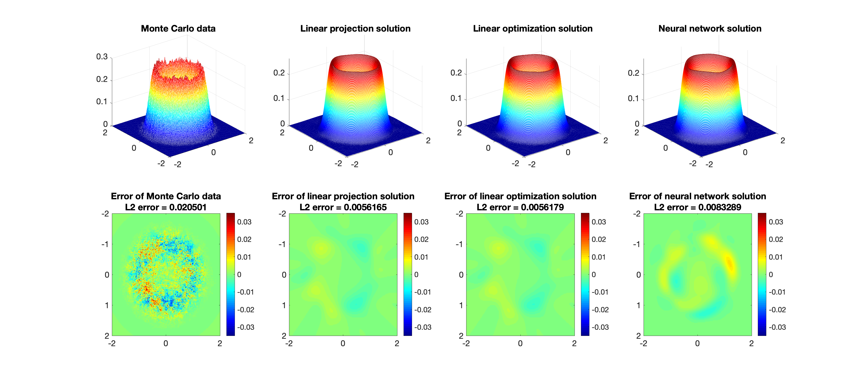
Figure 1. A comparison of probability density function of the invariant measure obtained by Monte Carlo simulation, linear projection method, linear optimization method, and optimization through an artificial neural network. First row: probability density functions. Second row: Distributions of error against the exact solution. (Grid size = $200\times 200$. Sample size of Monte Carlo: $10^{7}$.)

Our first goal is to compare the performance of the neural network representation, solution to the constrained optimization problem, and solution to the unconstrained optimization problem (2.5). In Figure 1, the first column gives a Monte Carlo approximation and its error distribution. As expected, the Monte Carlo approximation is both noisy and inaccurate. Note that the error term of the Monte Carlo approximation has very little spatial correlation. This motivates Assumption (A1). In the second and the third columns of Figure 1 respectively, we see the data-driven solvers (2.4) and (2.5) can clearly “smooth out” the fluctuation in the Monte Carlo approximation. This confirms the convergence result proved in [5] and Theorem 2.1. The last column of Figure 1 show that the artificial neural network method with loss function (3.1) has a similar “smoothing” effect. In the neural network training of this example, we let two sets of collocation points $\mathfrak{X}$ and $\mathfrak{Y}$ be the set of grid points to compare the result. This result validates the use of the loss function (3.1) as a continuous version of the unconstrained optimization problem (2.5). We can see when a grid-based approach is available, it usually has higher accuracy. However, the neural network method is more applicable to higher dimensional problems.

Instead of grid points, the second numerical simulation uses Algorithm 2 with randomly sample collocation points (using Algorithm 2). Figure 2 shows the neural network representations learnt from various amounts of reference points $v(\bm{y}_{j})$. The discrete $L^{2}$ errors is computed with respect to this grid and demonstrated on the title of each subfigures. The neural network is then trained with Algorithm 1, in which the norm of $\mathcal{L}u$ is evaluated at each training point. In order to numerically check the effect of the Fokker-Planck operator in the loss function, we train the neural network without calculating $\mathcal{L}u$, and demonstrate the result in Figure 3. More precisely, in Figure 3, we only use a large training data set $\mathfrak{Y}$. Step 3 in Algorithm 1 is skipped. See Appendix D.2 for details.

In Figure 2, we can see a clear underfitting when using too few reference points. The training result becomes satisfactory when the number of training points is $256$ or larger. As a comparison, if $\mathcal{L}u$ is not added to the loss function, one needs as large as $16384$ training points to reach the same accuracy. This shows the advantage of including $\mathcal{L}u$ into the loss function. The differential operator $\mathcal{L}u$ helps the neural network to find a solution to the Fokker-Planck equation. And the role of reference points is to make sure that the Fokker-Planck solution is the one we actually need. We can train the neural network with only a few hundreds reference points, and the accuracy of the probability density at those reference points does not have to be very high. Similarly to the discrete case in Theorem 2.1, the spatially uncorrelated noise can be effectively removed by training the loss function $L_{2}$. This observation is very important in practice, as in high dimension it is not practical to obtain the probability densities for a very large reference set, and the result from a high dimension Monte Carlo simulation is unlikely to be accurate.

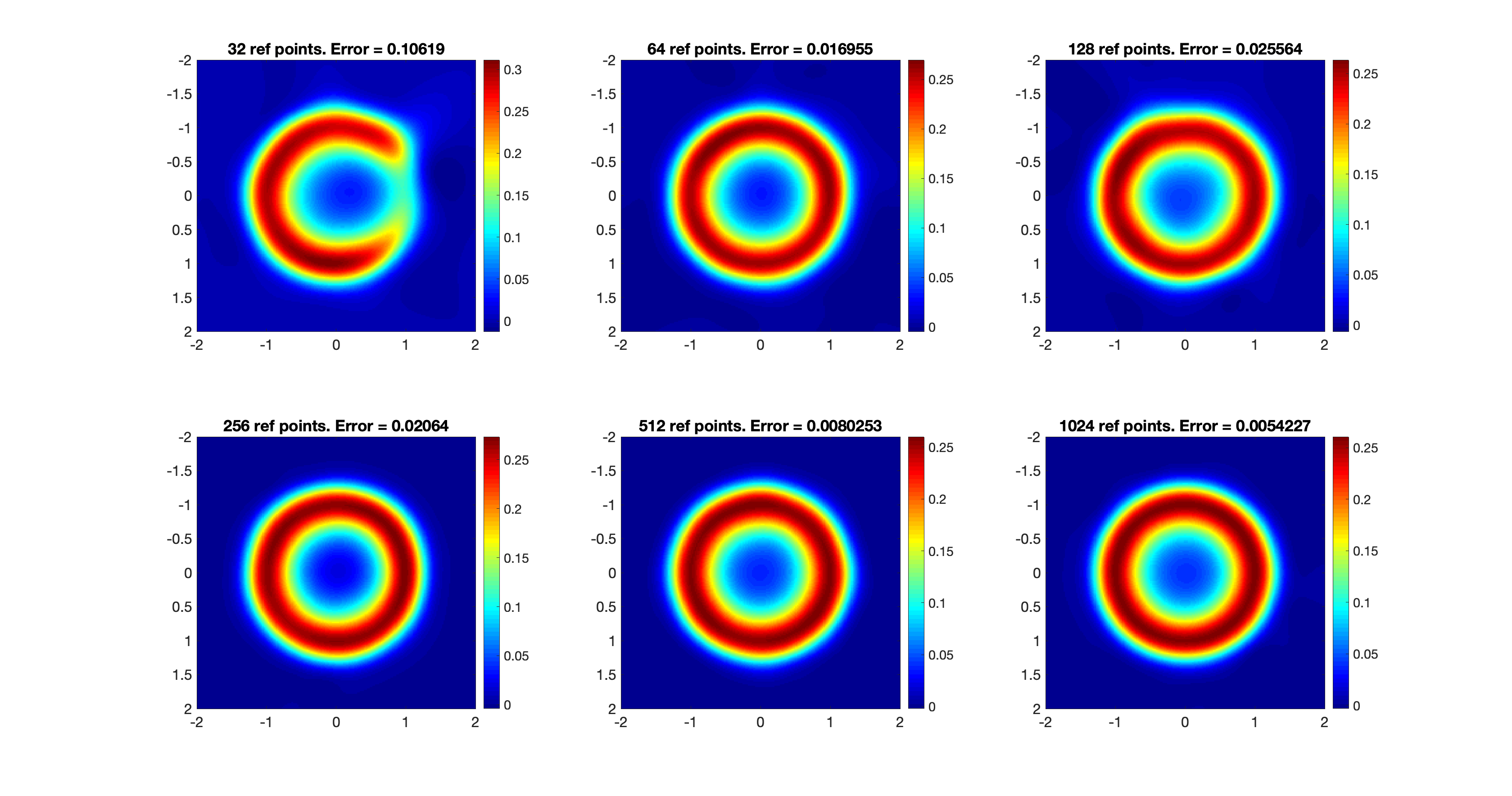
Figure 2. A comparison of different sizes of reference set with $\mathcal{L}u$ being in the loss function. Top left to bottom right: heat map of the invariant probability density function if the “ring model” with $32,64,128,256,512,$ and $1024$ reference points are used. The $L_{2}$ error is shown in the title of each subplot.

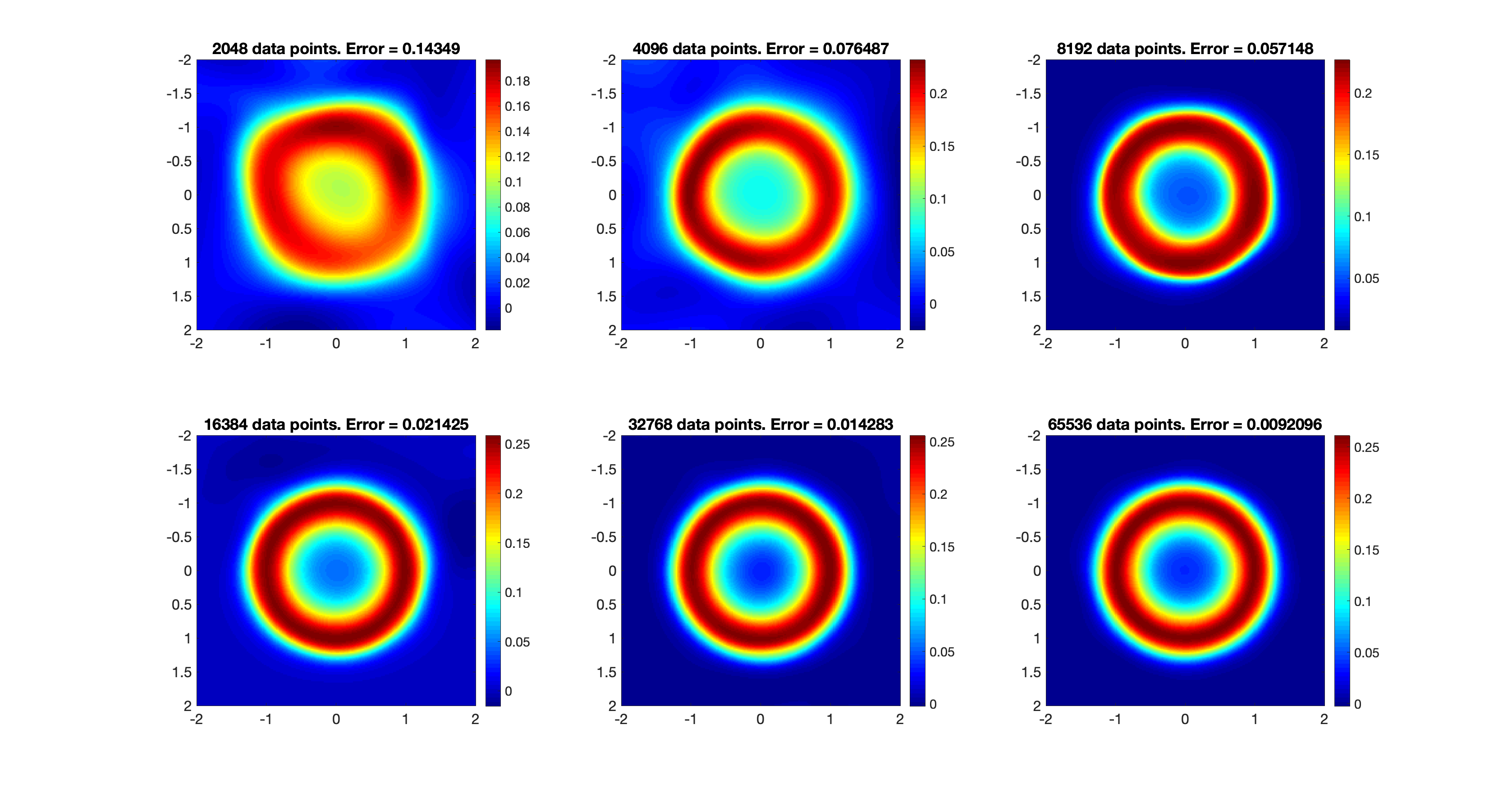
Figure 3. A comparison of different sizes of reference set without $\mathcal{L}u$ being in the loss function. Top left to bottom right: heat map of the invariant probability density function if the “ring model” with 2048, 4096, 8192, 16384, 32768, and 65536 reference points are used. The $L_{2}$ error is shown in the title of each subplot.

4.2. A 2D Gibbs measure

We consider a two dimensional stochastic gradient system

(4.2) $$\left\{\begin{array}[]{l}dX_{t}=(X_{t}^{2}Y_{t}-X_{t}^{5})\,dt+\sigma\,dW^{x}_{t},\\ dY_{t}=(\frac{1}{3}X_{t}^{3}-\frac{7}{3}Y_{t})\,dt+\sigma\,dW^{y}_{t},\end{array}\right.$$

where $W^{x}_{t}$ and $W^{y}_{t}$ are independent Wiener processes, and $\sigma=1$ in this example is the strength of the white noise. The drift part of equation (4.2) is a gradient flow of the potential function

$$V(x,y)=-\frac{1}{3}x^{3}y+\frac{1}{6}x^{6}+\frac{7}{6}y^{2}=\frac{1}{6}(x^{3}-y)^{2}+y^{2}.$$

So the invariant measure of (4.2) is the Gibbs measure with probability density function

$$u(x,y)=\frac{1}{Z}\exp(-2V(x,y)),$$

where $Z=\int_{-\infty}^{\infty}\int_{-\infty}^{\infty}\exp(-2V(x,y))\,dxdy$ is the normalization parameter. We choose this system because $Y_{t}$ is conditionally linear with respect to $X_{t}$. We can use this system to test the conditional Gaussian sampler.

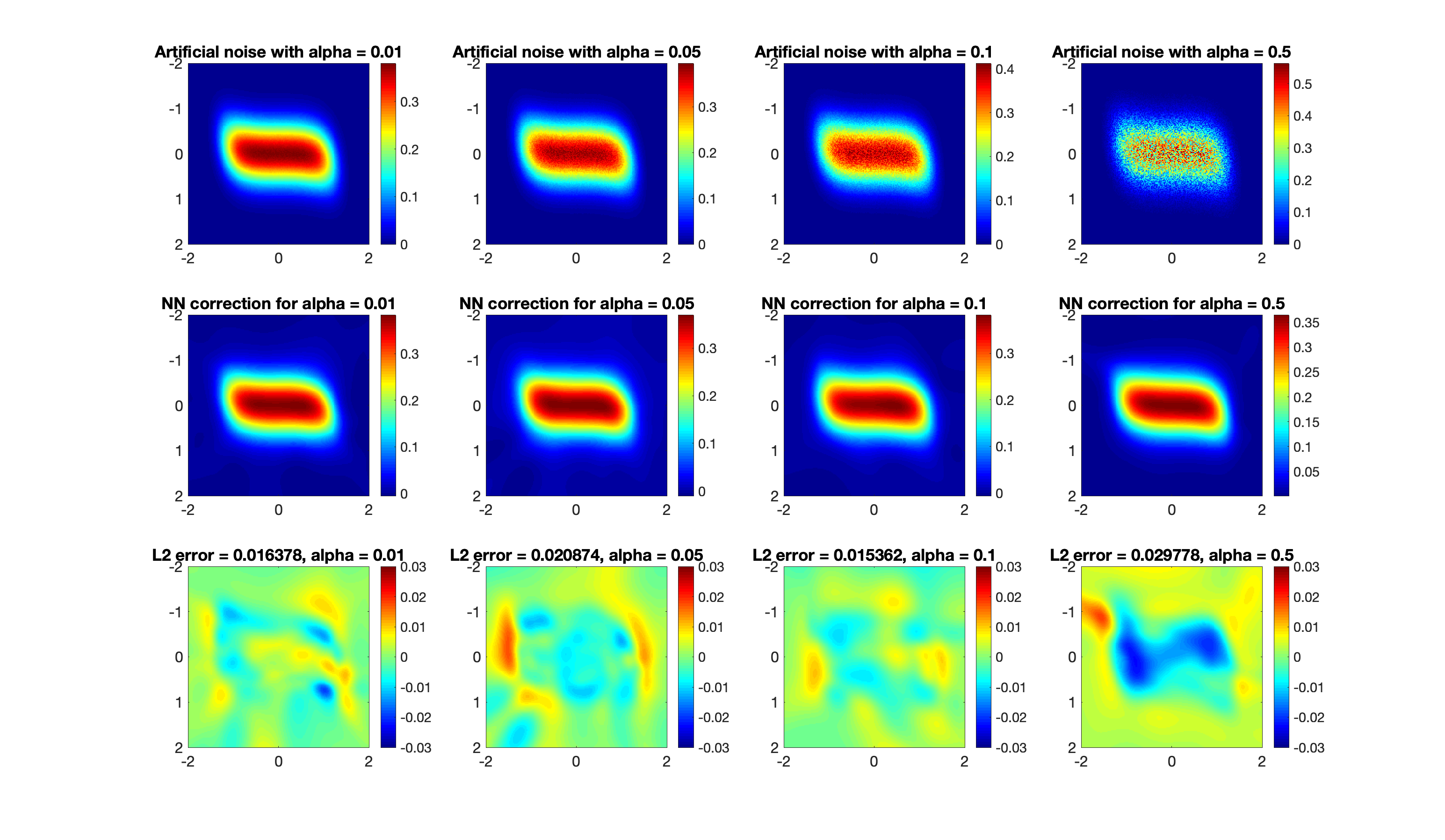
Figure 4. Neural network representations with different level of artificial noise. First row: Artificial noises added to the exact solution. Second row: Neural network approximation with $1024$ reference points and $10000$ training points. Third row: The error of the neural network approximation and the discrete $L_{2}$ error.

One aim of this numerical experiment is to show the unconstrained optimization problem used by the artificial neural network can tolerate spatially uncorrelated noise at a very high level. To demonstrate this, we artificially add a noise to the exact solution $u(x)$ of the Gibbs measure to get the reference data $v$. We first run Algorithm 2 to get four sets of collocation points $\bm{y}_{j},j=1,2,\dots,1024$. Then we generate four sets of reference data $v$ at these collocation points by injecting an artificial noise with maximal relative error $\alpha$, where $\alpha=0.01,0.05,0.1$, and $0.5$. Then we run Algorithm 1 with these sets of reference data $\{v({\bm{y}}_{j})\}_{j=1}^{1024}$. The first row of Figure 4 shows how the artificial noise is applied by increasing $\alpha$ and the second row shows the neural network approximation. Observing from the third row of Figure 4, it is surprising that even when the magnitude of the multiplicative noise is increased to $0.5$, namely, the relative error of the Monte Carlo approximation is $50\%$, the correction $\tilde{\bm{u}}(\cdot,\theta)$ is still quite accurate. This shows our method has high tolerance to spatially uncorrelated noise, which is usually the case of the reference data obtained from Monte Carlo simulations.

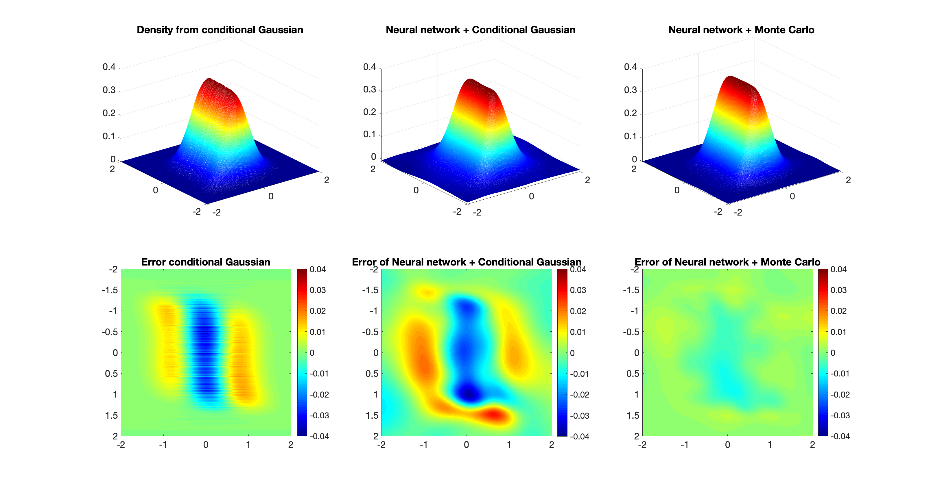
Figure 5. A comparison of the conditional Gaussian method and the direct Monte Carlo method. First column: The invariant probability density function and its error obtained by the conditional Gaussian method. Second column: Top: The invariant probability density function and its error obtained by the neural network approximation, with $1024$ training points whose densities are obtained by Algorithm 4. Bottom: The invariant probability density function and its error obtained by the neural network approximation, with $1024$ training points whose densities are obtained by Monte Carlo simulation.

Then we use the conditional Gaussian sampler (Algorithm 4 in Appendix C) to generate the probability density function. In Figure 5, we can see there is a small but systematic bias in the probability density function given by Algorithm 4. We suspect that this bias comes from the use of one long trajectory in Algorithm 4. As a result, if we use it to generate reference data $v(\bm{y}_{j})$ for ${\bm{y}}_{j}\in\mathfrak{Y}$, the error will be systematic, which is very different from the spatially uncorrelated noise seen in the Monte Carlo result. This systematic bias makes the differential operator $\mathcal{L}u$ in the loss function hard to guide the training, because there are infinitely many functions that solve $\mathcal{L}u=0$. To maintain a minimization of the two parts of the loss function (3.1), a balance between them forces the neural network approximation to produce an approximation biased from the exact solution. In other words, $\bm{e}=\bm{v}-\bm{u}^{*}$ as defined in Section 2.2 for this conditional Gaussian approximation does not satisfy Assumption (A1). Consequently, the convergence of $\mathbb{E}[\bm{z}]=\mathbb{E}[\bar{\bm{u}}-{\bm{u}}^{*}]$ is not guaranteed. However, the conditional Gaussian sampler has its advantage in higher dimensions. See Section 4.4 for more discussion.

4.3. A 4D ring density

Consider a generalization of the stochastic gradient system in Subsection 4.1 in four dimensional state space

(4.3) $$\left\{\begin{array}[]{l}dX_{t}=(-4X_{t}(X_{t}^{2}+Y_{t}^{2}+Z_{t}^{2}+U_{t}^{2}-1)+Y_{t})\,dt+\sigma\,dW^{x}_{t},\\ dY_{t}=(-4Y_{t}(X_{t}^{2}+Y_{t}^{2}+Z_{t}^{2}+U_{t}^{2}-1)-X_{t})\,dt+\sigma\,dW^{y}_{t},\\ dZ_{t}=(-4Z_{t}(X_{t}^{2}+Y_{t}^{2}+Z_{t}^{2}+U_{t}^{2}-1))\,dt+\sigma\,dW^{z}_{t},\\ dU_{t}=(-4U_{t}(X_{t}^{2}+Y_{t}^{2}+Z_{t}^{2}+U_{t}^{2}-1))\,dt+\sigma\,dW^{u}_{t},\end{array}\right.$$

where $W^{x}_{t},W^{y}_{t},W^{z}_{t}$ and $W^{u}_{t}$ are independent Wiener processes, and $\sigma=1$ in this example is the strength of the white noise. The drift part of equation (4.3) is a gradient flow of the potential function

$$V(x,y)=(x^{2}+y^{2}+z^{2}+u^{2}-1)^{2}$$

plus a rotation term orthogonal to the equipotential lines of $V$ in the first two dimensions of variables $x$ and $y$. Hence the invariant measure of (4.3) is

$$u(x,y,z,u)=\frac{1}{Z}\exp(-2V(x,y,z,u)),$$

where $Z=\int_{-\infty}^{\infty}\int_{-\infty}^{\infty}\int_{-\infty}^{\infty}\int_{-\infty}^{\infty}\exp(-2V(x,y,z,u))\,dxdydzdu$ is the normalization parameter. Similar to Subsection 4.1, the rotation term does not change the invariant probability density function, which can be verified by substituting $u(x,y,z,u)$ into the Fokker-Planck equation of (4.3).

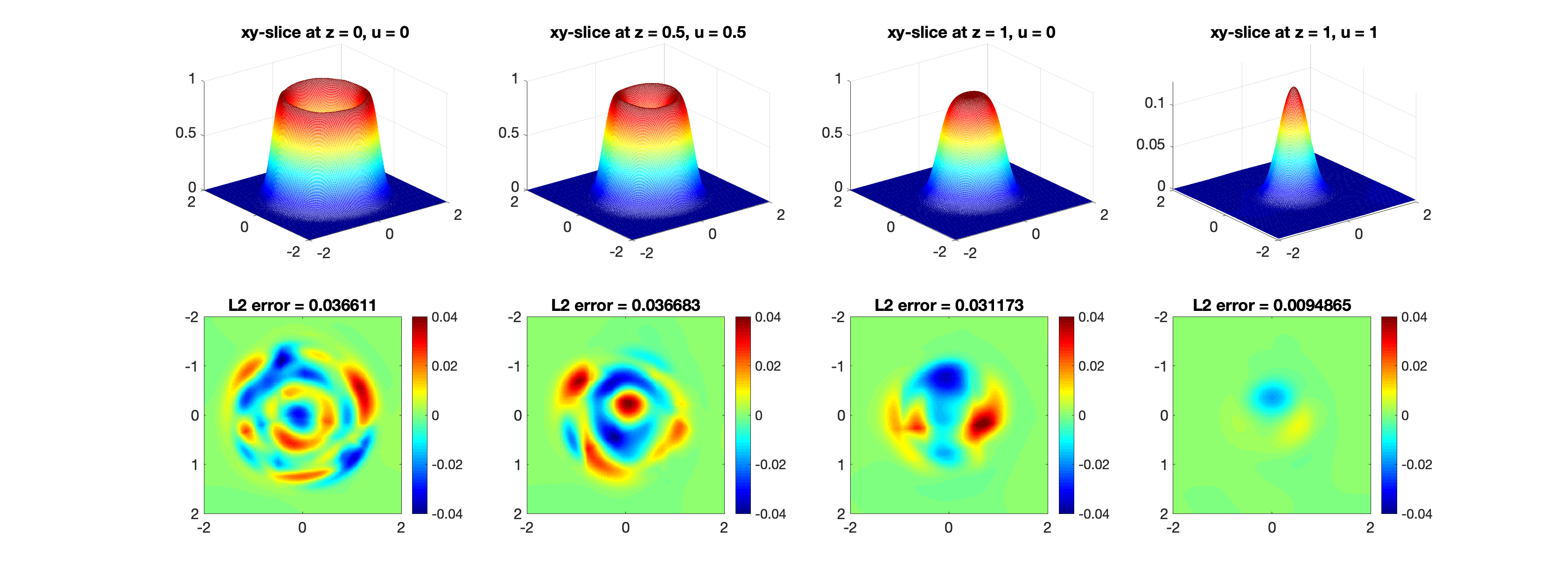
Figure 6. Invariant probability density function of the 4D ring (Equation (4.3)). Total number of reference points is 10000. Probability density at reference points is obtained by direct Monte Carlo method with $10^{10}$ sample points. First row: Invariant probability density functions restricted on the $x$-$y$ slices with $z=0,u=0$. $z=0.5,u=0.5$, $z=1,u=0$, and $z=1,u=1$. Second row: Error of probability density functions when comparing with the exact solution. The discrete $L_{2}$ error is shown in the title of each subplot.

The aim of this example is to demonstrate the accuracy of neural network representation in 4D. The numerical domain is $D=[-2,2]^{2}$. We use Algorithm 2 to sample $10^{4}$ reference points and $10^{5}$ training points. Probability densities at training points are obtained by Algorithm 3. After we get the neural network approximation by Algorithm 1, we evaluate it on the four $x$-$y$ slices for $(z,u)=(0,0),(0.5,0.5),(1,0)$ and $(1,1)$ in Figure 6. Figure 6 also shows the error distributions and the $L^{2}$ error on these slices. The errors at all points in these 4 slices are controlled at a very low level $\leq 0.04$. And the discrete $L^{2}$ errors are satisfactory. Figure 6 illustrates that after training the loss function (3.1) on a sparse set of reference data, this solution function is accurate at any point in $D$. It demonstrates strong representing power of the neural network approximation, both globally and locally. We remark that it is not possible to solve this 4D Fokker-Planck equation with traditional numerical PDE approach. The divide-and-conquer strategy in [5] would be difficult to implement as well, due to the high memory requirement of a 4D mesh.

4.4. A 6D conceptual dynamical model for turbulence

In this subsection, we consider a six dimensional stochastic dynamical system with conditional Gaussian structure as (C.1)-(C.2) with $\bm{X}^{l}_{\mathbf{I}}(t)=X_{t}$ and $\bm{X}^{l}_{\mathbf{II}}(t)=(Y^{(1)}_{t},Y^{(2)}_{t},Y^{(3)}_{t},Y^{(4)}_{t},Y^{(5)}_{t})^{T}$

(4.4) $$\left\{\begin{array}[]{l}dX_{t}=(-0.1X_{t}+0.5+0.25X_{t}(Y^{(1)}_{t}+Y^{(2)}_{t}+Y^{(3)}_{t}+Y^{(4)}_{t}+Y^{(5)}_{t}))\,dt+2\,dW^{x}_{t},\\ dY^{(1)}_{t}=(-0.2Y^{(1)}_{t}-0.25X_{t}^{2})\,dt+0.5\,dW^{(1)}_{t},\\ dY^{(2)}_{t}=(-0.5Y^{(2)}_{t}-0.25X_{t}^{2})\,dt+0.2\,dW^{(2)}_{t},\\ dY^{(3)}_{t}=(-Y^{(3)}_{t}-0.25X_{t}^{2})\,dt+0.1\,dW^{(3)}_{t},\\ dY^{(4)}_{t}=(-2Y^{(4)}_{t}-0.25X_{t}^{2})\,dt+0.1\,dW^{(4)}_{t},\\ dY^{(5)}_{t}=(-5Y^{(5)}_{t}-0.25X_{t}^{2})\,dt+0.1\,dW^{(5)}_{t},\end{array}\right.$$

where $W^{x}_{t}$ and $W^{(i)}_{t},i=1,2,\dots,5$, are independent Wiener processes. This model has been studied in [4] as a numerical example.

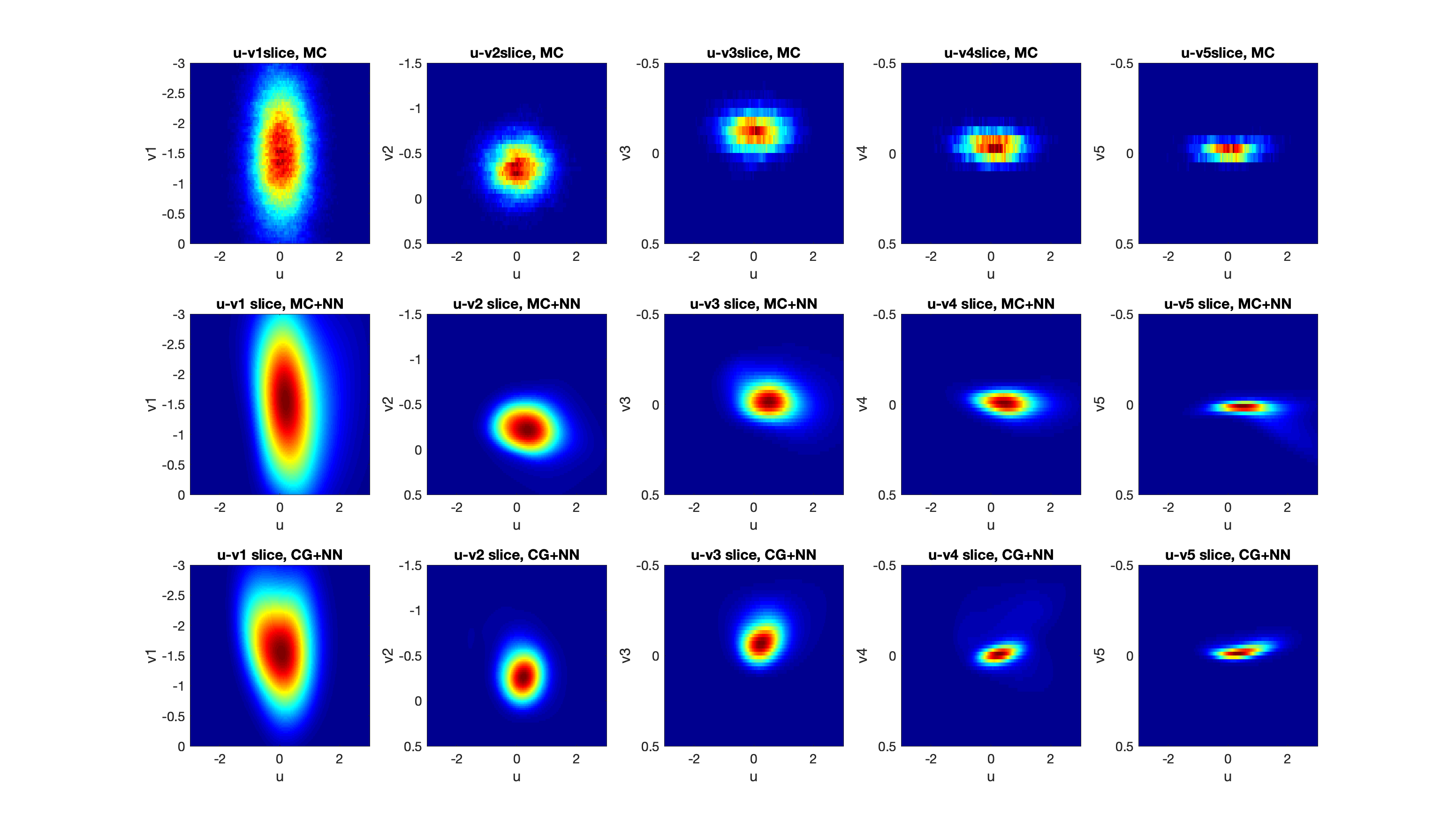
Figure 7. Heat maps of the invariant probability density function of the 6D turbulence model restricted on 2D slices. From left to right: the $i$th plot is the $u$-$v_{i},i=1,2,\dots,5$ slice with $v_{j}=0,j\neq i$. Top row are invariant probability density functions obtained by the direct Monte Carlo method. Middle row and bottom row are the neural network approximation using Algorithm 1 with probability densities $\{v({\bm{y}}_{i})\}$ obtained by Monte Carlo simulation and the conditional Gaussian sampler, respectively.

In this high dimensional system, we compare the direct Monte Carlo approximation and neural network approximation with the reference data obtained from both Monte Carlo and the modified conditional Gaussian sampler in Algorithm 4. It is not possible to visualize a 6D probability density function, so we compare probability densities on the central slices in the 6D state space, namely, the $u$-$v_{i},i=1,2,\dots,5$ hyperplanes with $v_{j}=0,j\neq i$. The first row demonstrates the probability density functions at the five slices obtained by a direct Monte Carlo simulation. The solution has low resolution and low accuracy because It is difficult to collect enough samples in high dimension.

In this example, we generate a reference point set $\mathfrak{Y}$ with size $N^{Y}=20000$ using Algorithm 2. These collocations are very sparse in this six dimensional region $D$. Then we use both Monte Carlo approximation and the conditional Gaussian sampler in Algorithm 4 to generate the probability density $v({\bm{y}}_{i})$ for ${\bm{y}}_{i}\in\mathfrak{Y}$. Note that the simulation time of Monte Carlo sampler is about $100$ times more than the conditional Gaussian sampler. Then in both cases, we use Algorithm 1 to obtain a neural network approximation of the invariant probability measure. After the neural network is trained in the whole region $D$, we evaluate and plot it on the five central slices (see the second and third row in Figure 7). Although a closed-form solution for this example is not possible, we can still see that the solution obtained by three different approaches are not very far away from each other. This confirms the validity of the solutions. The neural network has low demand ($20000$ points) on reference data points and fast training speed (less than one hour). After the training, we can use it to predict the invariant probability density at any point in the domain. This is a remarkable result, because it is impossible to solve such as six dimensional problem by using traditional approaches.

5. Conclusion and Prospective Works

We proposed a neural network approximation method for solving the Fokker-Planck equations. The motivation is that the data-driven method studied in [9, 5] can be converted to a similar unconstrained optimization problem, and a mesh-free neural network solver can be used to solve the “continuous version” of this unconstrained optimization problem. We only present the case of the stationary Fokker-Planck equation that describes the invariant probability measure, because the case of the time-dependent Fokker-Planck equation is analogous. By introducing the differential operator of the Fokker-Planck equation into the loss function, the demand for large training data in the learning process is significantly reduced. Our simulation shows that the neural network can tolerate very high noise in the training data so long as it is spatially uncorrelated. We believe this work provides an effective numerical approach to study many high dimensional stochastic dynamics.

In this paper, the convergence of minimizer of the new unconstrained optimization problem is only carried out for the discrete case. It is tempting to extend this result to the space of functions. The problem becomes trivial and not interesting if we work with the space of $C^{\infty}$ functions and assume that the error term of the Monte Carlo simulation is a spatial white noise. So we need to consider the more realistic case such as the Barron space, and find a more realistic assumption to describe the reference data obtained by the Monte Carlo simulation. We plan to carry out this study in our subsequent work. In the future, we will also apply this method to more complicated but interesting systems such as systems with non-Gaussian Lévy noises and quasi-stationary distributions.

Appendix A Proof of Theorem 2.1

We first need to describe how the “baseline” solution ${\bm{u}^{*}}$ is obtained. Let $\hat{\bm{u}}\in\mathbb{R}^{N^{n}}$ denote the true solution of the Fokker-Planck equation restricted on the rectangular grid $\{x_{i}\}_{i=1}^{N^{n}}$ in $D$, that is, $\hat{\bm{u}}_{i}$ is the solution to equation (2.2) at point $x_{i}$. Then ${\bm{u}}^{*}$ is the numerical solution obtained by the finite difference method such that ${\bm{A}}{\bm{u}}^{*}=0$ and ${\bm{u}}^{*}=\hat{\bm{u}}$ at all grid points on $\partial D$. More precisely, we need to solve a new linear system

$$\begin{bmatrix}{\bm{A}}\\ P_{0}\end{bmatrix}{\bm{u}}^{*}=\begin{bmatrix}{\bm{0}}\\ P_{0}\hat{\bm{u}}\end{bmatrix}\,,$$

where ${\bm{A}}$ is the aforementioned $(N-2)^{n}\times N^{n}$ matrix, $P_{0}$ is an $(N^{n}-(N-2)^{n})\times N^{n}$ matrix such that $P_{0}{\bm{u}}$ gives entries of ${\bm{u}}$ on grid points on $\partial D$. Since the finite difference method is convergent for second order elliptic PDEs with given boundary value, when $h\ll 1$, ${\bm{u}}^{*}$ is a good approximation of $\hat{\bm{u}}$. And the accuracy of ${\bm{u}}^{*}$ is considerable higher than the result of Monte Carlo simulations.

Proof of Theorem 2.1.

Let $F({\bm{u}})={\bm{u}}^{T}{\bm{A}}^{T}{\bm{A}}{\bm{u}}+(\bm{u}-\bm{v})^{T}(\bm{u}-\bm{v})$. It is easy to see that the minimizer solves

$$\frac{\partial F({\bm{u}})}{\partial{\bm{u}}}=2{\bm{A}}^{T}{\bm{A}}{\bm{u}}+2{\bm{u}}-2{\bm{v}}={\bm{0}}\,.$$

Therefore, the quadratic form (2.5) has a unique minimizer $\bar{\bm{u}}=(\bm{I}+\bm{A}^{T}\bm{A})^{-1}\bm{v}$.

Denote $\bm{B}=(\bm{I}+\bm{A}^{T}\bm{A})^{-1}$. Then

$$\bm{B}^{-1}\bm{u}^{*}=(\bm{I}+\bm{A}^{T}\bm{A})\bm{u}^{*}=\bm{u}^{*},$$

and

$$\bm{v}=\bm{B}^{-1}\bar{\bm{u}}=\bm{B}^{-1}\bar{\bm{u}}-\bm{B}^{-1}\bm{u}^{*}+\bm{u}^{*}=\bm{B}^{-1}\bm{z}+\bm{u}^{*}.$$

So $\bm{z}=\bm{B}\bm{e}$. Therefore, $\mathbb{E}[\bm{z}]=0$ by assumption (A1), and $\text{cov}(\bm{z},\bm{z})=\zeta^{2}\bm{B}\bm{B}^{T}=\zeta^{2}\bm{B}^{2}$ by the symmetry of $\bm{B}$. Furthermore,

$$\mathbb{E}[\|\bm{z}\|^{2}_{2}]=\text{Trace}(\text{cov}(\bm{z},\bm{z}))=\zeta^{2}\text{Trace}(\bm{B}^{2})=\zeta^{2}\sum_{k=1}^{M}\lambda_{k}^{2},$$

where $M=N^{n}$ and $\{\lambda_{k}\}_{k=1}^{M}$ are the eigenvalues of $\bm{B}$.

For the sake of simplicity let $M=N^{n}$. Recall that ${\bm{A}}_{h}=h^{2}{\bm{A}}$. Since $\bm{A}_{h}^{T}\bm{A}_{h}$ is symmetric, there is a orthonormal matrix $\bm{Q}$ such that $\bm{A}_{h}^{T}\bm{A}_{h}=\bm{Q}\bm{\Lambda}_{h}\bm{Q}^{T}$, where $\bm{\Lambda}_{h}=\text{diag}\{\lambda^{h}_{1},\cdots\lambda^{h}_{M}\}$ is the diagonal matrix whose diagonal elements are the eigenvalues of $\bm{A}_{h}^{T}\bm{A}_{h}$. A short calculation shows

$$\lambda_{k}=\frac{1}{1+h^{-4}\lambda^{h}_{k}}\,.$$

Since $\bm{A}_{h}^{T}\bm{A}_{h}$ is positive semi-definite and $\bm{A}_{h}\in\mathbb{R}^{(N-2)^{n}\times N^{n}}$ has full rank, $\bm{A}_{h}^{T}\bm{A}_{h}$ has $N^{n}-(N-2)^{n}$ zero eigenvalues, while $r=(N-2)^{n}$ eigenvalues are positive. So for all sufficiently small $h>0$, we have

$$\mathbb{E}[\|\bm{z}\|^{2}_{2}] =\zeta^{2}\sum_{k=1}^{M}\lambda_{k}^{2}=\zeta^{2}\sum_{k=1}^{M}\left(\frac{1}{1+h^{-4}\lambda^{h}_{k}}\right)^{2}$$

$$=\zeta^{2}\left[N^{n}-(N-2)^{n}+\sum_{i=1}^{r}\left(\frac{1}{1+h^{-4}\lambda^{h}_{i}}\right)^{2}\right]\,.$$

Since $\mathbb{E}[\|{\bm{e}}\|^{2}]=\zeta^{2}N^{n}$ and $N=O(h^{-1})$, by Assumption (A2), we have

$$\frac{\mathbb{E}[\|\bm{z}\|^{2}_{2}]}{\mathbb{E}[\|{\bm{e}}\|^{2}]}\leq\frac{N^{n}-(N-2)^{n}}{N^{n}}+O(1)Q(h)\rightarrow 0$$

as $h\rightarrow 0$. ∎

It remains to discuss why Assumption (A2) is a valid assumption. Because ${\bm{A}}$ is obtained by finite difference method, it has the form $\bm{A}=h^{-2}(\bm{A_{0}}(h)+h\bm{A_{1}}(h))$, where ${\bm{A}_{0}}$ (resp. ${\bm{A}_{1}}$) is a constant matrix if $\sigma$ (resp. $f$) is constant. It is extremely difficult to rigorously prove Assumption (A2) when $\sigma$ and $f$ in equation (2.1) are location-dependent. In general, the smallest nonzero eigenvalue is $O(h^{4})$, but other eigenvalues are significantly larger than $O(h^{4})$. There are $O(h^{-n})$ terms in the summation in the definition of $Q(h)$. Hence $Q(h)$ approaches to zero when $h\ll 1$. In Figure 8, we numerically verify Assumption (A2) for 1D and 2D Fokker-Planck equations. We can see that $Q(h)\rightarrow 0$ as $h\rightarrow 0$ in both cases. This numerical result is for $\sigma=\mathrm{Id}_{n}$ and $f=0$. Note that $f$ determines ${\bm{A}_{1}}(h)$, which is only a small perturbation of the matrix ${\bm{A}}(h)$. So we expect Assumption (A2) to hold for any bounded $f$.

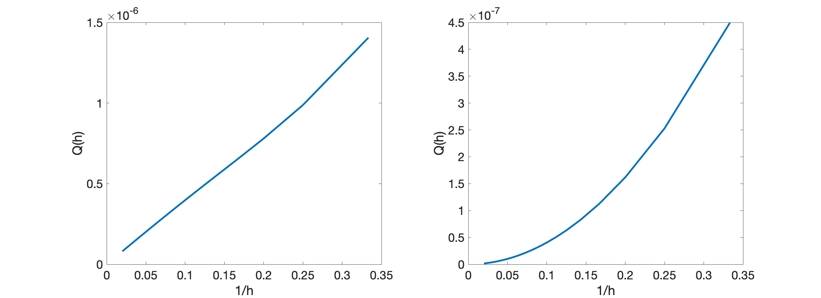
Figure 8. Left: $Q(h)$ vs. $h$ for the discretized 1D Fokker-Planck operator. Right: $Q(h)$ vs. $h$ for the discretized 2D Fokker-Planck operator.

Appendix B Sampling probability densities – direct Monte Carlo.

It remains to discuss the sampling technique to obtain ${\bm{v}(y_{i})}$ for ${\bm{y}_{i}}\in\mathfrak{Y}$. This step is trivial when using traditional grid-based method. One only needs to set up a grid in the numerical domain and count sample points in the neighborhood of each grid from a long trajectory. However, instead of the full space, Algorithm 1 only requires probability densities at thousands of reference points ${\bm{y}_{i}}\in\mathfrak{Y}$. Also a high dimensional grid could occupy an unrealistic amount of memory. So we need to improve the efficiency of the Monte Carlo sampler.

As mentioned in Section 2.1, to obtain a desirable accuracy of the reference data $v(\bm{y}_{j})$ using a Monte Carlo method, one needs to run very long numerical trajectories of (2.1) to guarantee enough points on the trajectories are counted around $\bm{y}_{j}$. On the other hand, when the dimensionality increases, the size of reference set $\mathfrak{Y}$ in the training process also increases. For example, to solve a 6D Fokker-Planck equation, $N^{Y}$ needs to be as large as tens of thousands. If we do not optimize the algorithm, then every time a new sample point is obtained from a long trajectory, one must check whether it belongs to the neighborhood of each collocation points $\bm{y}_{j}\in\mathfrak{Y}$. This will make the long trajectory sampler too slow to be useful.

An alternative approach is to create an $N$ mesh with $N^{n}$ grid points on $D=\prod_{\iota=1}^{n}[a_{\iota},b_{\iota}]$ and denote the vector of grid points by $\bm{y}^{k},k=1,2,\dots,N^{n}$. Let $h_{\iota}=(b_{iota}-a_{iota})/h$ be the grid size. This gives an $n$-dimensional “box” $\prod_{\iota=1}^{n}[{\bm{y}}^{k}_{\iota}-h_{\iota},{\bm{y}}^{k}_{\iota}+h_{\iota}]$ around each mesh point ${\bm{y}}^{k}$. Instead of using Algorithm 2 to sample $\bm{y}_{j}$ directly, we choose the closest mesh point $\bm{y}^{k_{j}}$ for each $\bm{y}_{j}$ given by Algorithm 2. So we have $\mathfrak{Y}=\{\bm{y}^{k_{j}}\},j=1,\cdots,N^{Y}$. With the help of the mesh, we can put a sample point into the corresponding $n$-dimensional “box” after implementing $2n$ comparisons. After running a sufficiently long trajectory, the number of samples in each box gives the approximate probability density at each grid point. Then we can look up the probability density of $\bm{y}^{k_{j}}$ from the corresponding boxes. This approach dramatically improves the efficiency, at the cost of storing a big array with $N^{n}$ points. When $n\geq 4$, this method could have an unrealistically high demand of the memory.

We propose the following “splitting” method to balance the efficiency and the memory pressure. The idea is to split the dimensions in to groups to reduce the size of vector stored in the memory. To be specific, we use $n=6$ as an example to state this method. One can easily generalize it to other dimensions. For $\mathbb{R}^{6}=\mathbb{R}^{3}\times\mathbb{R}^{3}$, we create an array of arrays $\mathcal{Q}$ with $2\times N^{3}$ entries. The first and second $N^{3}$ entries are for the first and second $\mathbb{R}^{3}$, respectively. Each entry of $\mathcal{Q}$ is an array of indices of training points. More precisely, for a collocation point $\bm{y}_{j}=(y^{j}_{1},y^{j}_{2},\dots,y^{j}_{6})\in\mathfrak{Y}$ that is also a mesh point, we denote its index by $(n_{1},n_{2},\dots,n_{6})$, where $n_{\iota}=(y^{j}_{\iota}-a_{\iota})/h_{j},\iota=1,2,\dots,6$. Then we record the numbering $j$ in two arrays corresponding to the $(n_{1}N^{2}+n_{2}N+n_{3})$-th and the $(N^{3}+n_{4}N^{2}+n_{5}N+n_{6})$-th entries of $\mathcal{Q}$. When a sample point $\bm{x}=(x_{1},x_{2},\dots,x_{6})$ is obtained from the Monte Carlo sampler, we compute its mesh index $(n^{\bm{x}}_{1},n^{\bm{x}}_{2},\dots,n^{\bm{x}}_{6})$, where $n^{\bm{x}}_{\iota}=\lfloor(x_{\iota}-a_{\iota})/h_{\iota}+1/2\rfloor,\iota=1,2,\dots,6$. Then we check the arrays at the $(n^{\bm{x}}_{1}N^{2}+n^{\bm{x}}_{2}N+n^{\bm{x}}_{3})$-th and the $(N^{3}+n^{\bm{x}}_{4}N^{2}+n^{\bm{x}}_{5}N+n^{\bm{x}}_{6})$-th entries of $\mathcal{A}$. The sample point ${\bm{x}}$ is associated to the training point ${\bm{y}}_{j}$ if and only if the intersection of the two aforementioned arrays is $j$. See Algorithm 3 for the full detail.

Algorithm 3 Reference data sampling with Monte Carlo method for high dimensional spaces $\mathbb{R}^{6}$

1:Reference set $\mathfrak{Y}=\{{\bm{y}}_{1},\cdots,{\bm{y}}_{N^{Y}}\}$. ${\bm{y}}_{i}$ are grid points.

2:Probability densities $v(\bm{y}_{j})$ at $\bm{y}_{j},j=1,2,\dots,N^{Y}$.

3:Set a zero array $\bm{\eta}$ with length $N^{Y}$ and an array of arrays $\mathcal{Q}$ that contains $2\times N^{3}$ empty arrays.

4:Sample $N^{Y}$ collocation points using Algorithm 2

5:for $j=1$ to $N^{Y}$ do

6:     Compute $n_{\iota}=(y^{j}_{\iota}-a_{\iota})/h_{\iota},\iota=1,2,\dots,6$.

7:     Add $j$ to the $(n_{1}N^{2}+n_{2}N+n_{3})$-th and the $(N^{3}+n_{4}N^{2}+n_{5}N+n_{6})$-th elemental arrays of $\mathcal{Q}$.

8:end for

9:Initialize $\bm{X}(0)$ and run a numerical simulation of equation (2.1)) for sometime $t_{0}$ and “burn in” time $t_{0}$.

10:Reset $\bm{X}(0)=\bm{X}(t_{0})$

11:for $l=1$ to $L$ do

12:     Continue the numerical simulation of (2.1) with step size $\Delta t$ to get a new sample point $\bm{x}=\bm{X}(l\Delta t)$.

13:     Compute $n^{\bm{x}}_{\iota}=\lfloor(x_{\iota}-a_{\iota})/h_{\iota}+1/2\rfloor,\iota=1,2,\dots,6$.

14:     Check the intersection $\mathcal{B}_{\bm{x}}$ of the $(n^{\bm{x}}_{1}N^{2}+n^{\bm{x}}_{2}N+n^{\bm{x}}_{3})$-th and the $(N^{3}+n^{\bm{x}}_{4}N^{2}+n^{\bm{x}}_{5}N+n^{\bm{x}}_{6})$-th elemental arrays of $\mathcal{Q}$.

15:     if $\mathcal{B}_{\bm{x}}=\{j\}$ then

16:         $\bm{\eta}(j)=\bm{\eta}(j)+1$.

17:     end if

18:end for

19:Return $v(\bm{y}_{j})=\bm{\eta}(j)\prod_{\iota=1}^{6}h_{\iota}^{-1}/L,j=1,2,\dots,N^{Y}$.

Appendix C Sampling probability densities – conditional Gaussian sampler.

As discussed before, the direct Monte Carlo method still suffers from the curse of dimensionality. It is more and more difficult to collect enough samples in a higher dimensional box. To maintain the desired accuracy in high dimensional spaces, the requirement of sampling grows exponentially with the dimension. We need to either run much longer numerical trajectories of (2.1) or make the grid more coarse. Otherwise the simulation will give a lot of $v({\bm{y}}_{i})=0$ at reference points ${\bm{y}_{i}}$ whose invariant probability density is not zero. This makes it not applicable as a reference data in the neural network training. For some high dimensional problems with conditional linear structure, the conditional Gaussian framework introduced in [3, 4] can be effectively applied to solve the problem of curse-of-dimensionality. Consider a stochastic differential equation with the following the conditional linear structure

(C.1) $$d\bm{X}_{\mathbf{I}} =[\bm{A}_{0}(t,\bm{X}_{\mathbf{I}})+\bm{A}_{1}(t,\bm{X}_{\mathbf{I}})\bm{X}_{\mathbf{II}}]\,dt+\bm{\Sigma}_{\mathbf{I}}(t,\bm{X}_{\mathbf{I}})\,d\bm{W}_{\mathbf{I}}(t),$$

(C.2) $$d\bm{X}_{\mathbf{II}} =[\bm{a}_{0}(t,\bm{X}_{\mathbf{I}})+\bm{a}_{1}(t,\bm{X}_{\mathbf{I}})\bm{X}_{\mathbf{II}}]\,dt+\bm{\Sigma}_{\mathbf{II}}(t,\bm{X}_{\mathbf{I}})\,d\bm{W}_{\mathbf{II}}(t),$$

where $\bm{X}(t)=(\bm{X}_{\mathbf{I}}(t),\bm{X}_{\mathbf{II}}(t))\in\mathbb{R}^{n_{\mathbf{I}}}\times\mathbb{R}^{n_{\mathbf{II}}}$ is the solution stochastic process. Then given the current path $\bm{X}_{\mathbf{I}}(s),s\leq t$, the conditional distribution of $\bm{X}_{\mathbf{II}}(t)$ is approximated by a Gaussian distribution

$$(\bm{X}_{\mathbf{II}}(t)|\bm{X}_{\mathbf{I}}(s),s\leq t)\sim N(\,\overline{\!{\bm{X}}}_{\mathbf{II}}(t),\bm{R}_{\mathbf{II}}(t)),$$

where the expectation $\,\overline{\!{\bm{X}}}_{\mathbf{II}}(t)$ and variance $\bm{R}_{\mathbf{II}}(t)$ follow the ordinary differential equations

(C.3) $$d\,\overline{\!{\bm{X}}}_{\mathbf{II}} =[\bm{a}_{0}+\bm{a}_{1}\,\overline{\!{\bm{X}}}_{\mathbf{II}}]\,dt+(\bm{R}_{\mathbf{II}}\bm{A}_{1}^{*}(\bm{\Sigma}_{\mathbf{I}}\bm{\Sigma}_{\mathbf{I}}^{*})^{-1}[d\bm{X}_{\mathbf{I}}-(\bm{A}_{0}+\bm{A}_{1}\,\overline{\!{\bm{X}}}_{\mathbf{II}})\,dt],$$

(C.4) $$d\bm{R}_{\mathbf{II}} =[\bm{a}_{1}\bm{R}_{\mathbf{II}}+\bm{R}_{\mathbf{II}}\bm{a}_{1}^{*}+(\bm{\Sigma}_{\mathbf{I}}\bm{\Sigma}_{\mathbf{I}}^{*})-(\bm{R}_{\mathbf{II}}\bm{A}_{1}^{*}(\bm{\Sigma}_{\mathbf{I}}\bm{\Sigma}_{\mathbf{I}}^{*})^{-1}(\bm{R}_{\mathbf{II}}\bm{A}_{1}^{*})^{*}]\,dt.$$

The original algorithm in [4] is for simulating the time evolution of the probability density function. The probability density function is obtained by averaging the conditional probability density of many independent trajectories of equation (2.1). Since the focus of this paper is the invariant probability density function, we make some modification to the conditional Gaussian framework in [4]. The main difference is that we use one long trajectory to simulate the conditional probability density. This is because the speed of convergence of the evolution of transient distribution to the invariant distribution of equation (2.1) is unknown. In a simulation, we don’t know when the probability density function becomes a satisfactory approximation of the invariant probability density function.

In equation (C.1)-(C.2), the first part $\bm{X}_{\mathbf{I}}$ is usually in a relatively low dimension $n_{\mathbf{I}}$. So for this part, a Monte Carlo approximation is reliable. Let $\mathfrak{Y}$ be the set of reference points. Denote the two coordinates of a reference point ${\bm{y}}_{i}\in\mathfrak{Y}$ by ${\bm{y}}_{i}^{\mathbf{I}}$ and ${\bm{y}}_{i}^{\mathbf{II}}$ respectively. Then we run a long numerical trajectory $\bm{X}$, for (C.1)-(C.2) and evaluate the trajectory at discrete times $0=t_{0}<t_{1}<t_{2}<\cdots<t_{I}=T$. Denote the visiting times of $\bm{X}_{\mathbf{I}}$ to an $h$-neighborhood of ${\bm{y}}_{i}^{\mathbf{I}}$ by $t_{k_{1}},\cdots,t_{k_{S(j)}}$. Then at time $t_{k_{i}}$, the conditional probability density of at ${\bm{y}}_{i}^{\mathbf{II}}$ is

(C.5) $$\begin{array}[]{ll}v_{i,j}&=f_{(\bm{y}^{\mathbf{II}}_{j}(t_{k_{i}})|\bm{y}^{\mathbf{I}}_{j}(s),s\leq t_{k_{i}})}(\bm{y}^{\mathbf{II}}_{j})\\ &=\frac{1}{\sqrt{(2\pi)^{n_{\mathbf{II}}}|\bm{R}_{\mathbf{II}}(t_{k_{i}})|}}\exp(-\frac{1}{2}(\bm{y}^{\mathbf{II}}_{j}-\,\overline{\!{\bm{X}}}_{\mathbf{II}}(t_{k_{i}}))^{T}\bm{R}_{\mathbf{II}}(t_{k_{i}})^{-1}(\bm{y}^{\mathbf{II}}_{j}-\,\overline{\!{\bm{X}}}_{\mathbf{II}}(t_{k_{i}})))\end{array}$$

according to the Gaussian distribution $N(\,\overline{\!{\bm{X}}}_{\mathbf{II}}(t_{k_{i}}),\bm{R}_{\mathbf{II}}(t_{k_{i}}))$.This gives a more reliable approximation for the reference data $v(\bm{y}_{j})$

(C.6) $$v(\bm{y}_{j})=\frac{1}{S(j)}\sum_{i=1}^{S(j)}v_{i,j}.$$

See Algorithm 4 for the full detail.

Algorithm 4 Reference data sampling for high dimensional spaces with conditional Gaussian structure

1:Conditional linear stochastic differential equations (C.1) and (C.2).

2:Reference approximation $v(\bm{y}_{j})$ at $\bm{y}_{j}=(\bm{y}^{\mathbf{I}}_{j},\bm{y}^{\mathbf{II}}_{j}),j=1,2,\dots,N^{Y}$.

3:Initialize $\bm{X}(0)$ and run a numerical simulation of equation (C.1)-(C.2) for sometime $t_{0}$ and “burn in”.

4:Reset $\bm{X}(0)=\bm{X}(t_{0})$

5:Continue the numerical simulation of (2.1) for a relatively large $T$ and collect $\bm{X}_{\mathbf{I}}(s),s\leq t$.

6:Run a numerical solver for (C.3) and (C.4) to get $\,\overline{\!{\bm{X}}}_{\mathbf{II}}(t)$ and $\bm{R}_{\mathbf{II}}(t)$.

7:for $j=1$ to $M$ do

8:     Record $\bm{X}(t_{k_{i}}),i=1,2,\dots,S(j)\in B(\bm{y}^{\mathbf{I}}_{j},h)$ in $\mathbb{R}^{n_{\mathbf{I}}}$.

9:     Evaluate $v_{k,j}$ using (C.5).

10:end for

11:Return $v(\bm{y}_{j}),j=1,2,\dots,N^{Y}$ using (C.6).

Appendix D Numerical simulation details

D.1. Parameter of the neural network.

Throughout this paper, we use a small feed-forward neural network with $6$ hidden layers, each of which contains $16,128,128,128,16,4$ neurons respectively, to approximate the solution to Fokker-Planck equation in all numerical examples. The output layer always has one neuron. Number of neurons in the input layer depends on the problem. All activation functions are the sigmoid function. We choose sigmoid function because (1) the solution of the Fokker-Planck equation is everywhere nonnegative and (2) the second order derivative of the neural network output is included in the loss function.

D.2. Numerical example 1.

In Figure 1, the Monte Carlo solution is obtained by running an Euler-Maruyama numerical scheme for (4.1) with $10^{7}$ steps and calculating the empirical probability on a $200\times 200$ mesh of the region $D=[-2,2]\times[-2,2]$. The time step size is $0.001$. Optimization problems in equation (2.4) and (2.5) are solved by linear algebra solvers. The neural network training with loss function 3.1 uses all probability densities at grid points obtained by the same Monte Carlo simulation. The architecture of the artificial neural network is described in Section D.1 with two input neuron and one output neuron.

In Figure 2, Algorithm 2 is used to generate reference points and training points. The number of reference points in six panels of Figure 2 are $32,64,128,256,512$, and $1024$ respectively. The number of training points is $10000$ in all cases. All probability densities $v({\bm{y}}_{i})$ at training points are obtained by Algorithm 3, which runs the Euler-Maruyama scheme for $10^{8}$ steps. Then we train the artificial neural network with loss function (3.1). The architecture of the artificial neural network is described in Section D.1 with two input neuron and one output neuron. The trained neural network is evaluated on a $400\times 400$ grid.

When generating Figure 3, we use the loss function without $\mathcal{L}u$, so there is no training set $\mathfrak{X}$. In six panel of Figure 3, the numbers of reference points $v(\bm{y}_{j})$ with probability densities are 2048, 4096, 8192, 16384, 32768, and 65536, respectively. Reference points are obtained by Algorithm 2. The probability density at each reference point is exact (obtained from the Gibbs density). The architecture of the artificial neural network is described in Section D.1 with two input neuron and one output neuron. The trained neural network is evaluated on a $400\times 400$ grid.

D.3. Numerical example 2.

In Figure 4, Algorithm 2 is used to generate $1024$ reference points and $10000$ training points. Then we artificially inject some noise into the training data. For a reference point ${\bm{y}}_{i}\in\mathfrak{Y}$, we have $v_{i}(\bm{y}_{j})=r_{i}(\bm{y}_{j})u(\bm{y}_{j})$, where $u$ is the Gibbs density, $r_{i}\sim U([1-\alpha,1+\alpha])$ is a random variable uniformly distributed in a range $[1-\alpha,1+\alpha]$. Here, $\alpha$ controls the “strength” of the artificial noise. Four different values $\alpha=0.01,0.05,0.1$ and $0.5$ are used to generate four different reference data sets $\{v({\bm{y}}_{j})\}_{j=1}^{1024}$. The architecture of the artificial neural network is described in Section D.1 with two input neuron and one output neuron. The trained neural network is evaluated on a $400\times 400$ grid.

In Figure 5, the conditional Gaussian simulation is obtained by running Algorithm 4. The trajectory is recorded at $50000$ discrete times. The probability density at $400\times 400$ grid points are evaluated by using Algorithm 4. (Two panels in the first column). Next, Algorithm 2 is used to generate $1024$ reference points and $10000$ training points. The probability densities at those training points are evaluated by running Algorithm 4 (same sample size as above) and Algorithm 3, respectively. Two sets of probability densities at reference points are used in the neural network training (with loss function (3.1)) to generate subplots in the second and third column, respectively. The architecture of the artificial neural network is described in Section D.1 with two input neuron and one output neuron. The trained neural network is evaluated on a $400\times 400$ grid.

D.4. Numerical example 3.

In Figure 6, algorithm 2 is used to sample $10000$ reference points and $10^{5}$ training points in the domain $D=[-2,2]^{4}$. Then we run algorithm 3 with $10^{10}$ steps of the Euler-Maruyama scheme to estimate the probability densities at training points. The values of the probability density function are rescaled on the whole domain $D$ such that the maximum is $1$ (for otherwise the neural network cannot easily learn the distinction among small values). Then we train the artificial neural network with loss function (3.1). The architecture of the artificial neural network is described in Section D.1 with four input neuron and one output neuron. The trained neural network is evaluated at four $(x,y)$-slices for $(z,u)=(0,0),(0.5,0.5),(1,0)$ and $(1,1)$ respectively. Each $(x,y)$ slice contains $400\times 400$ grid points.

D.5. Numerical example 4.

In Figure 7, the numerical domain is $[-3,3]\times[-3,0]\times[-1.5,0.5]\times[-0.5,0.5]\times[-0.5,0.5]\times[-0.5,0.5]\subset\mathbb{R}^{6}$. A direct Monte Carlo simulation that uses $8\times 10^{9}$ steps of Euler-Maruyama scheme is used to generate subplots in the first row. The grid size of the Monte Carlo simpler is $0.05$. Then we use Algorithm 2 to sample $20000$ reference points and $10^{5}$ training points in the domain $D$. Two sets of probability densities at reference points are obtained using two approaches. The first approach uses Algorithm 3 with $4\times 10^{10}$ steps of the Euler-Maruyama scheme. The second approach uses $8\times 10^{5}$ samples from the conditional Gaussian sampler in Algorithm 4. The values of the probability density function are rescaled on the whole domain $D$ such that the maximum is $1$. Then we train two artificial neural networks (with loss function (3.1)) using the same collocation points but two sets of probability densities at reference points. The results are shown in the second and third row of Figure 7 respectively. The architecture of the artificial neural network is described in Section D.1 with six input neuron and one output neuron. The trained neural network is evaluated at five $(u,v_{i})$-slices for $i=1,\cdots,5$ centering at the origin.

References

- [1] Christian Beck, Sebastian Becker, Philipp Grohs, Nor Jaafari, and Arnulf Jentzen, Solving stochastic differential equations and Kolmogorov equations by means of deep learning, arXiv:1806.00421, 2018.
- [2] Christian Beck, Weinan E, and Arnulf Jentzen, Machine learning approximation algorithms for high-dimensional fully nonlinear partial differential equations and second-order backward stochastic differential equations, Journal of Nonlinear Science 29 (2019), 1563–1619.
- [3] Nan Chen and Andrew J Majda, Beating the curse of dimension with accurate statistics for the Fokker-Planck equation in complex turbulent systems, Proceedings of the National Academy of Sciences 114 (2017), no. 49, 12864–12869.
- [4] by same author, Efficient statistically accurate algorithms for the Fokker-Planck equation in large dimensions, Journal of Computational Physics 354 (2018), 242–268.
- [5] Matthew Dobson, Yao Li, and Jiayu Zhai, An efficient data-driven solver for Fokker-Planck equations: algorithm and analysis, arXiv:1906.02600, 2019.
- [6] Weinan E, Chao Ma, and Lei Wu, Barron spaces and the compositional function spaces for neural network models, arXiv:1906.08039, 2019.
- [7] Ingo Gühring, Gitta Kutyniok, and Philipp Petersen, Error bounds for approximations with deep ReLU neural networks in norms, Analysis and Applications 18 (2020), no. 5, 803–859.
- [8] Diederik P. Kingma and Jimmy Ba, Adam: A method for stochastic optimization, 3rd International Conference on Learning Representations, ICLR 2015, San Diego, CA, USA, May 7-9, 2015, Conference Track Proceedings (Yoshua Bengio and Yann LeCun, eds.), 2015.
- [9] Yao Li, A data-driven method for the steady state of randomly perturbed dynamics, Communications in Mathematical Sciences 17 (2019), no. 4, 1045–1059.
- [10] Philipp Petersen and Felix Voigtlaender, Optimal approximation of piecewise smooth functions using deep ReLU neural networks, Neural Networks 108 (2018), 296–330.
- [11] Maziar Raissi, Paris Perdikaris, and George Em Karniadakis, Physics-informed neural networks: A deep learning framework for solving forward and inverse problems involving nonlinear partial differential equations, Journal of Computational Physics 378 (2019), 586–707.
- [12] Justin Sirignano and Konstantinos Spiliopoulos, Dgm: A deep learning algorithm for solving partial differential equations, Journal of Computational Physics 375 (2018), 1339–1364.
- [13] Taiji Suzuki, Adaptivity of deep reLU network for learning in besov and mixed smooth besov spaces: optimal rate and curse of dimensionality, International Conference on Learning Representations, 2019, arXiv:1810.08033.
- [14] Jin-Long Wu, Heng Xiao, and Eric Paterson, Physics-informed machine learning approach for augmenting turbulence models: A comprehensive framework, Phys. Rev. Fluids 3 (2018), 074602.