Testing General Relativity with NuSTAR data of Galactic Black Holes

Abstract

Einstein’s theory of General Relativity predicts that the spacetime metric around astrophysical black holes is described by the Kerr solution. In this work, we employ state-of-the-art relativistic reflection modeling to analyze a selected set of NuSTAR spectra of Galactic black holes to obtain the most robust and precise constraints on the Kerr black hole hypothesis possible today. Our constraints are much more stringent than those from other electromagnetic techniques, and with some sources we find stronger constraints than those currently available from gravitational waves.

1. Introduction

The theory of General Relativity was proposed at the end of 1915 (Einstein, 1916) and so far has successfully passed a large number of observational tests. The theory has been extensively tested in the weak-field regime with experiments in the Solar System and observations of binary pulsars (Will, 2014). The past five years have seen tremendous progress in the study of the strong-field regime and we can now test the predictions of General Relativity with gravitational waves (e.g., Abbott et al., 2016; Yunes et al., 2016; Abbott et al., 2019), X-ray data (e.g., Cao et al., 2018; Tripathi et al., 2019, 2020), and mm and sub-mm Very Long Baseline Interferometry (VLBI) observations (e.g., Psaltis et al., 2020).

In General Relativity and in the absence of exotic matter fields, the spacetime metric around astrophysical black holes should be described well by the Kerr solution (Kerr, 1963). This is the result of the black hole uniqueness theorems in General Relativity (see, e.g., Chruściel et al., 2012) and of the fact that deviations induced by a possible accretion disk, nearby stars, or a black hole non-vanishing electric charge are normally negligible (see, e.g., Bambi et al., 2014; Bambi, 2018). However, macroscopic deviations from the Kerr metric are predicted in a number of scenarios with new physics, including models with macroscopic quantum gravity effects (e.g., Giddings, 2017), models with exotic matter fields (e.g., Herdeiro & Radu, 2014), or in the case General Relativity is not the correct theory of gravity (e.g., Kleihaus et al., 2011). Testing the Kerr metric around astrophysical black holes is thus a test of General Relativity in the strong field regime (but see Psaltis et al., 2008).

We note that electromagnetic and gravitational wave tests are, in general, complementary because they can probe different sectors of the theory (Bambi, 2017). Electromagnetic tests are more suitable to verify the interactions between the gravity and the matter sectors, including particle motion and non-gravitational interactions in a gravitational field (Will, 2014). Gravitational wave tests can probe the gravitational sector itself in the strong and dynamical regime.

The aim of the present work is to analyze the most suitable X-ray data of black holes to test the Kerr black hole hypothesis and to get the most robust constraints possible with the available observational data and theoretical models. Our astrophysical system is shown in Fig. 1 (see, e.g., Bambi et al., 2020). We have a black hole surrounded by a geometrically thin and optically thick cold (up to a few keV for stellar-mass black holes) accretion disk. Every point on the disk emits a blackbody-like spectrum and the whole disk has a multi-temperature blackbody-like spectrum. Thermal photons from the disk inverse Compton scatter off free electrons in the so-called corona, which is a hotter ($\sim$100 keV) gas close to the black hole and the inner part of the accretion disk. The Comptonized photons have a power-law spectrum with a high-energy cutoff and can illuminate the disk, producing the reflection spectrum. The latter is characterized by some fluorescent emission lines in the soft X-ray band, notably the iron K$\alpha$ complex peaked at $\sim$6 keV, and by a Compton hump peaked at 20-30 keV (Ross & Fabian, 2005; García & Kallman, 2010). In the presence of high-quality data and employing the correct astrophysical model, the analysis of these reflection features emitted from the inner part of the accretion disk can be a powerful tool to probe the strong gravity region near the black hole event horizon (Reynolds, 2019; Bambi et al., 2020).

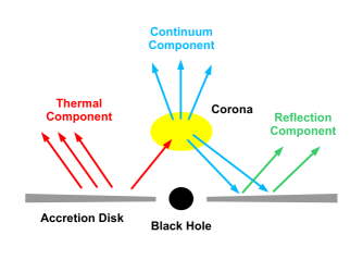
Figure 1.— A black hole is accreting from a geometrically thin and optically thick disk. The disk has a multi-temperature blackbody-like spectrum. Thermal photons from the disk inverse Compton scatter off free electrons in the corona, producing the continuum component. The latter illuminates the disk, generating the reflection component.

The paper is organized as follows. In Section 2, we present our selection of sources and observations. Section 3 is devoted to the data reduction and analysis. In Section 4, we discuss our results and we compare our constraints with those obtained from mm and sub-mm VLBI observations and from gravitational waves. In our study, we employ the Johannsen metric with the deformation parameter $\alpha_{13}$ (Johannsen, 2013); its expression is reported in Appendix A. In principle, we could use any other stationary, axisymmetric, and asymptotically flat non-Kerr black hole metric to constrain the associated deformation parameter and quantify possible deviations from the Kerr geometry. However, rotating black hole solutions beyond General Relativity are normally known either in numerical form or in an expansion on the spin parameter. Since our model currently works only with analytic metrics and we want to analyze the spectra of fast-rotating objects, with spin parameter close to 1, here we have employed a phenomenological metric. We also note that so far our efforts have been mainly focused to improve the astrophysical model to limit/understand the systematic uncertainties, thus devoting less attention to the capabilities of X-ray reflection spectroscopy of constraining specific gravity theories.

2. Selection of the sources/observations

The study of relativistic reflection features can be used to test the Kerr metric around either stellar-mass black holes in X-ray binaries and supermassive black holes in active galactic nuclei (AGN). We note that in some theoretical models deviations from the Kerr metric can be more easily detected in one of the two object classes than in the other one. For example, in higher-curvature theories, such as dynamical Chern-Simons and Einstein-dilaton-Gauss-Bonnet, observations of stellar-mass black holes normally lead to much stronger constraints than those of supermassive black holes, because the curvature at the black hole horizon is inversely proportional to the square of the black hole mass (Yagi & Stein, 2016). We also note that tests with X-ray binaries have some advantages over AGN. The sources are brighter, and so have better statistics. The spectra of AGN often present warm absorbers, which may introduce astrophysical uncertainties in the measurement. In this study, we thus focus on stellar-mass black holes.

NuSTAR (Harrison et al., 2013) is the most suitable X-ray mission for the study of relativistic reflection features of black hole binaries. The data are not affected by pile-up from the brightness of the sources and cover a broad energy band from 3 to 79 keV, so they permit us to analyze both the iron line and the Compton hump. Our starting point is thus the list of all published spin measurements of stellar-mass black holes with NuSTAR data (assuming the Kerr metric) obtained by studying the reflection features of the source. This list is shown in Tab. 1 and we see fourteen objects.

Source	$a_{*}$	Mission(s)	State	Reference
4U 1630–472	$0.985_{-0.014}^{+0.005}$	NuSTAR	Intermediate	King et al. (2014)
Cyg X-1	$>0.83$	NuSTAR+Suzaku	Soft	Tomsick et al. (2014)
	$>0.97$	NuSTAR+Suzaku	Hard	Parker et al. (2015)
	$0.93\sim 0.96$	NuSTAR	Soft	Walton et al. (2016)
EXO 1846–031	$0.997_{-0.002}^{+0.001}$	NuSTAR	Hard intermediate	Draghis et al. (2020)
GRS 1716–249	$>0.92$	NuSTAR+Swift	Hard Intermediate	Tao et al. (2019)
GRS 1739–278	$0.8\pm 0.2$	NuSTAR	Low/Hard	Miller et al. (2015)
GRS 1915+105	$0.98\pm 0.01$	NuSTAR	Low/Hard	Miller et al. (2013)
GS 1354–645	$>0.98$	NuSTAR	Hard	El-Batal et al. (2016)
GX 339–4	$0.95_{-0.08}^{+0.02}$	NuSTAR+Swift	Very High	Parker et al. (2016)
MAXI J1535–571	$>0.84$	NuSTAR	Hard	Xu et al. (2018a)
MAXI J1631–479	$>0.94$	NuSTAR	Soft	Xu et al. (2020)
Swift J1658.2–4242	$>0.96$	NuSTAR+Swift	Hard	Xu et al. (2018b)
Swift J174540.2–290037	$0.92_{-0.07}^{+0.05}$	Chandra+NuSTAR	Hard	Mori et al. (2019)
Swift J174540.7–290015	$0.94_{-0.10}^{+0.03}$	Chandra+NuSTAR	Soft	Mori et al. (2019)
V404 Cyg	$>0.92$	NuSTAR	Hard	Walton et al. (2017)

Table 1List of all published spin measurements of stellar-mass black holes obtained from NuSTAR data and from the analysis of relativistic reflection features of the sources. The fourth column refers to source state during the observation used for the spin measurement. All these spectral states are explicitly mentioned in reference papers in the last column except for V404 Cyg. The spectra of V404 Cyg in Walton et al. (2017) exhibit a very hard power-law ($\Gamma\approx 1.4$) and a weak disk blackbody component, so they can be classified in the hard state.

We want to now select the best sources and observations to get robust tests of the Kerr metric, as some sources/data are problematic and our result could be affected by systematic uncertainties not under control. Cyg X-1 is a complicated source because it is a high mass X-ray binary and the spectrum of the accretion disk of the black hole is strongly absorbed by the wind of the companion star. In the observation of GRS 1716–249 it is unclear whether the disk extends up to the innermost stable circular orbit (ISCO) or is truncated at a somewhat larger radius (Jiang et al., 2020). GRS 1915+105 is another well-known complicated source, where outflows from the accretion disk can absorb the X-ray radiation emitted from the region near the black hole. The observation of MAXI J1535–571 is affected by dust scattering. MAXI J1631–497 was observed in the soft state, where our reflection model for cold disks may have some problem, and the reflection spectrum is strongly affected by a variable and extremely fast disk wind. Swift J174540.2 and Swift J174540.7 are two X-ray transients within 1 pc from Sgr A*, which makes a precise measurement of these sources quite challenging (it is even under debate whether these sources are indeed black hole binaries or not). V404 Cyg is another very complicated source characterized by strong and extremely variable absorption. Eventually, we remain with six sources more suitable (even if not all ideal) for tests of the Kerr black hole hypothesis: 4U 1630–472, EXO 1846–031, GRS 1739–278, GS 1354–645, GX 339–4, and Swift J1658–4242.

3. Data reduction and analysis

3.1. Data reduction

Source	Observation ID	Observation Date	Exposure (ks)	Counts [s-1]
4U 1630–472	40014009001	2013 May 9	14.6	77.5
EXO 1846–031	90501334002	2019 August 3	22.2	148.7
GRS 1739–278	80002018002	2014 March 26	29.7	127.8
GS 1354–645	90101006004	2015 July 11	30.0	51.8
GX 339–4	80001015003	2015 March 11	30.0	208.5
	00081429002	2015 March 11	1.9	35.4
Swift J1658–4242	90401307002	2018 February 16	33.3	34.5
	00810300002	2018 February 16	3.0	4.9

Table 2Summary of the sources and the observations analyzed in the present work.

The observations of the six selected sources are listed in Tab. 2. In the case of GX 339–4 and Swift J1658–4242, the first observation ID refers to the NuSTAR observation, the second one to the Swift observation. We note that these data of GS 1354–645 and GX 339–4 were already analyzed with an earlier version of our reflection model in Xu et al. (2018c) and Tripathi et al. (2021), respectively, but we repeat the analysis here with the latest version of our model (which, among other things, is more accurate for high inclination angles) in order to be able to consistently combine the measurements from the six sources together.

The raw data of the NuSTAR detectors FPMA and FPMB are processed to get cleaned events using the script nupipeline of NuSTAR data analysis Software (NustarDAS) v2.0.0, which is a part of spectral analysis HEASOFT v6.28. We use the latest calibration database CALDB v20200912. The source region, which varies from source to source, is selected such that 90% of its photons lie within. The background region, which has a similar size to the source region, is selected far from the source to avoid inclusion of source photons. The spectrum, ancillary, and response files are created using the module nuproducts of NuSTARDAS.

For the XRT/Swift data, the raw data are processed to cleaned event files using the xrtpipeline script of XRT/Swift data analysis Software (SWXRTDAS) v3.5.0 and CALDB v20200724. The source and background regions are selected in a similar way explained above for the NuSTAR data. The cleaned event files are then used to extract source and background spectra using xselect v2.4g. Ancillary files are generated using xrtmkarf and response matrices are taken from CALDB.

Finally, the source spectrum is grouped depending on the brightness of the source so that $\chi^{2}$ statistics can be applied. XSPEC v12.11.1 is used for spectral analysis and, in what follows, all the errors quoted are at 1-$\sigma$ unless stated otherwise.

3.2. Data analysis

3.2.1 Individual measurements

First, we analyze every source separately. We start by fitting the data with an absorbed power-law (an absorbed power-law + disk blackbody spectrum in the case of GX 339–4) and we show the data to best-fit model ratios for the six sources in Fig. 2. For every source, we clearly see a broad iron line and a Compton hump, indicating that we have a relativistically blurred reflection spectrum. In the case of 4U 1630–472, there is strong absorption at the iron line, but we can still determine that a broad iron line is there.

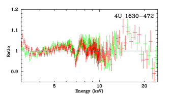
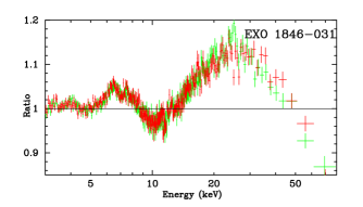
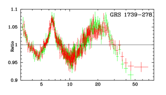
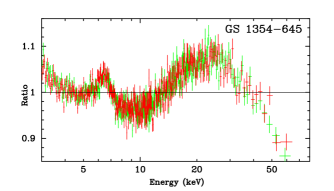
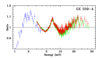
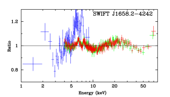
Figure 2.— Data to best-fit model ratio for an absorbed power-law (an absorbed power-law + disk blackbody spectrum in the case of GX 339–4) for the spectra analyzed in this work. Green crosses are for FPMA/NuSTAR data, red crosses are for FPMB/NuSTAR data, and blue crosses are for XRT/Swift data.

For the analysis of the reflection spectrum, we employ relxill_nk (Bambi et al., 2017; Abdikamalov et al., 2019), which is an extension of the relxill package (Dauser et al., 2013; García et al., 2014) to non-Kerr spacetimes. The model and its parameters are briefly reviewed in Appendix B. We use the latest version of relxill_nk, corresponding to v1.4.0. In the case of GX 339–4, the spectrum presents a prominent thermal component of the accretion disk, and thus we also use nkbb (Zhou et al., 2019). relxill_nk and nkbb are the state-of-the-art in, respectively, reflection and thermal models in non-Kerr spacetimes. In our analysis, we assume that the spacetime around these black holes can be described by the Johannsen metric (Johannsen, 2013) with the possible non-vanishing deformation parameter $\alpha_{13}$, while all other deformation parameters are set to zero (see Appendix A for more details). $\alpha_{13}$ is thus used to quantify possible deviations from the Kerr background, which is recovered for $\alpha_{13}=0$. From the analysis of the NuSTAR data of these six sources we want to estimate $\alpha_{13}$ and see whether it is consistent with zero, as is necessary to recover the Kerr metric and is predicted by General Relativity.

We proceed to find the best model for every source. Note that we cannot directly fit the data with the model published in literature for the spin measurement in the Kerr metric because, in principle, deviations from the Kerr background may be able to explain the data with different spectral components. However, we note that eventually we use the best models already used for the spin measurements of these sources, which can be explained with the fact that deviations from the Kerr background due to a non-vanishing $\alpha_{13}$ have their own impact on the spectrum and do not affect the choice of the final model (but such a conclusion may not hold for other deformations from the Kerr metric). Eventually we fit the data with the models listed in Tab. 3.

Source	Model
4U 1630–472	tbabs$\times$xstar$\times$relxilllpCp_nk
EXO 1846–031	tbabs$\times$(diskbb + relxill_nk + gaussian)
GRS 1739–278	tbabs$\times$relxill_nk
GS 1354–645	tbabs$\times$relxillCp_nk
GX 339–4	tbabs$\times$(nkbb + comptt + relxilllp_nk)
Swift J1658.2–4242	tbnew$\times$xstar$\times$(nthComp + relxilllpCp_nk + gaussian)

Table 3List of the models used for every source.

Since even for a single source we have several free parameters in the model, we run Markov Chain Monte-Carlo (MCMC) analyses. We use the python script by Jeremy Sanders employing emcee (MCMC Ensemble sampler implementing Goodman & Weare algorithm). Our results are shown in Tab. 4, where the reported uncertainties correspond to 1-$\sigma$ (for $\alpha_{13}$ we also show the 3-$\sigma$ estimate). The best-fit models and the data to best-fit model ratios of our six sources are shown in Fig. 3. The corner plots resulting from the MCMC analyses are shown in Figs. 4-9.

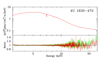
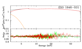
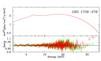
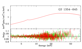
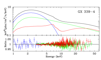
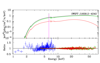
Figure 3.— Best-fit model and data to best-fit model ratio for the spectra analyzed in this work. For the best-fit model plots, the black curve (when present) refers to the total model, the red curve to the relativistic reflection spectrum described by relxill(lp)(Cp)_nk, the orange curve (in EXO 1846–031) to the thermal component described by diskbb, the blue curve (in GX 339–4) to the thermal model nkbb, the green curve to the continuum comptt (in GX 339–4) or nthComp (in Swift J1658.2–4242), and the magenta curve (in Swift J1658.2–4242) is an emission line. In the ratio plots, green crosses are for FPMA/NuSTAR data, red crosses are for FPMB/NuSTAR data, and blue crosses are for XRT/Swift data.

	4U 1630–472	EXO 1846–031	GRS 1739–278	GS 1354–645	GX 339–4	Swift J1658.2–4242
tbabs
$N_{\rm H}$ [$10^{22}$ cm-2]	$5.59^{+0.18}_{-0.13}$	$10.9^{+0.4}_{-0.3}$	$1.92^{+0.15}_{-0.14}$	$0.7^{*}$	$0.88^{+0.02}_{-0.02}$	$21.4^{+0.7}_{-0.6}$
	–	–	$1.70^{+0.15}_{-0.15}$	–	–	–
xstar
$N_{\rm H}$ [$10^{22}$ cm-2]	$35.6^{+1.9}_{-5.9}$	–	–	–	–	$79.3^{+0.3}_{-0.3}$
$\log\xi$ [erg cm s-1]	$4.96^{+0.03}_{-0.05}$	–	–	–	–	$4.84^{+0.12}_{-0.21}$
diskbb
$kT_{\rm in}$ [keV]	–	$0.427^{+0.007}_{-0.009}$	–	–	–	–
nkbb
$M$ [$M_{\odot}$]	–	–	–	–	$12.4^{+1.4}_{-0.7}$	–
$\dot{M}$ [$10^{18}$ g/s]	–	–	–	–	$0.73^{+0.11}_{-0.07}$	–
$D$ [kpc]	–	–	–	–	$10.4^{+1.8}_{-1.0}$	–
comptt
$kT_{0}$ [keV]	–	–	–	–	$0.355^{+0.014}_{-0.011}$	–
$kT_{\rm plasma}$ [keV]	–	–	–	–	$181^{+5}_{-6}$	–
$\tau$	–	–	–	–	$<0.01$	–
nthComp
$kT_{0}$ [keV]	–	–	–	–	–	$0.1^{*}$
$kT_{\rm plasma}$ [keV]	–	–	–	–	–	$38.6^{+0.7}_{-0.7}$
relxill(lp)(Cp)_nk
$h$ $[r_{\rm g}]$	$2.24^{+0.07}_{-0.08}$	–	–	–	$8.0^{+0.5}_{-0.4}$	$2.07^{+0.17}_{-0.05}$
$q_{\rm in}$	–	$7.3^{+0.6}_{-0.6}$	$6.4^{+0.3}_{-0.3}$	$8.9^{+0.8}_{-1.2}$	–	–
$q_{\rm out}$	–	$0.4^{+0.4}_{-0.3}$	$2.10^{+0.05}_{-0.04}$	$0.4^{+0.4}_{-0.3}$	–	–
$R_{\rm br}$ [$r_{\rm g}$]	–	$7.4^{+1.5}_{-1.4}$	$5.70^{+0.21}_{-0.39}$	$5.4^{+1.2}_{-0.9}$	–	–
$a_{*}$	$0.990^{+0.003}_{-0.005}$	$0.9968^{+0.0015}_{-0.0017}$	$0.975^{+0.014}_{-0.018}$	$0.992^{+0.004}_{-0.004}$	$0.9944^{+0.0009}_{-0.0015}$	$0.955^{+0.024}_{-0.022}$
$i$ [deg]	$8^{+6}_{-4}$	$73.4^{+1.3}_{-1.3}$	$15^{+3}_{-3}$	$74.1^{+1.7}_{-2.5}$	$28.5^{+0.78}_{-0.7}$	$64.9^{+1.1}_{-1.6}$
$\Gamma$	$1.40^{+0.04}_{-0.03}$	$2.002^{+0.018}_{-0.013}$	$1.21^{+0.02}_{-0.02}$	$1.67^{+0.02}_{-0.03}$	$2.10^{+0.03}_{-0.03}$	$1.667^{+0.008}_{-0.023}$
$E_{\rm cut}$ [keV]	–	$198^{+4}_{-5}$	$25.3^{+0.5}_{-0.4}$	–	$2gkT_{\rm plasma}$	–
$kT_{\rm e}$ [keV]	$2.42^{+0.09}_{-0.08}$	–	–	$146^{+13}_{-13}$	–	$gkT_{\rm plasma}$
$\log\xi$ [erg cm s-1]	$2.36^{+0.10}_{-0.08}$	$3.47^{+0.04}_{-0.03}$	$3.50^{+0.03}_{-0.03}$	$2.05^{+0.04}_{-0.04}$	$3.63^{+0.05}_{-0.04}$	$2.73^{+0.18}_{-0.16}$
$A_{\rm Fe}$	$1^{*}$	$0.85^{+0.05}_{-0.05}$	$3.3^{+0.4}_{-0.3}$	$0.60^{+0.06}_{-0.05}$	$5.9^{+0.4}_{-0.4}$	$0.95^{+0.23}_{-0.31}$
$R_{\rm f}$	$1.35^{+0.15}_{-0.14}$	$1^{*}$	$0.45^{+0.05}_{-0.07}$	$0.31^{+0.03}_{-0.04}$	–	–
$\alpha_{13}$	$-0.03^{+0.08}_{-0.06}$	$-0.03^{+0.03}_{-0.06}$	$-0.31^{+0.20}_{-0.25}$	$-0.04^{+0.16}_{-0.15}$	$-0.023^{+0.015}_{-0.026}$	$-0.05^{+0.44}_{-0.47}$
$\alpha_{13}$ (3$\sigma$)	$-0.03^{+0.63}_{-0.18}$	$-0.03^{+0.17}_{-0.18}$	$-0.31^{+0.64}_{-0.53}$	$-0.04^{+0.58}_{-0.87}$	$-0.023^{+0.030}_{-0.137}$	$-0.05^{+1.21}_{-0.97}$
gaussian
$E_{\rm line}$	–	$7.01^{+0.04}_{-0.04}$	–	–	–	$6.29^{+0.02}_{-0.03}$
$\chi^{2}_{\nu}$	1224.01/1084	2751.90/2594	1285.84/1112	2895.14/2720	869.15/647	1741.78/1644
	=1.1292	=1.0609	=1.1563	=1.0644	=1.3434	=1.0595

Table 4Summary of the best-fit values of the six sources analyzed in this work.

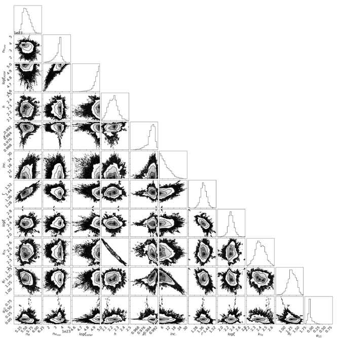
Figure 4.— Corner plot for the free parameter-pairs (excluding calibration constants and component normalization) for 4U 1630–472 after the MCMC run. The 2D plots report the 1-, 2-, and 3-$\sigma$ confidence contours.

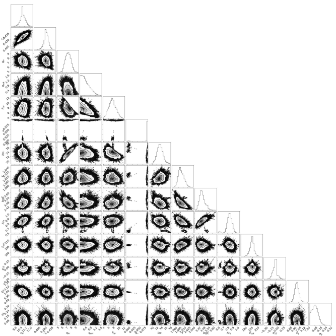
Figure 5.— As in Fig. 4 for EXO 1846–031.

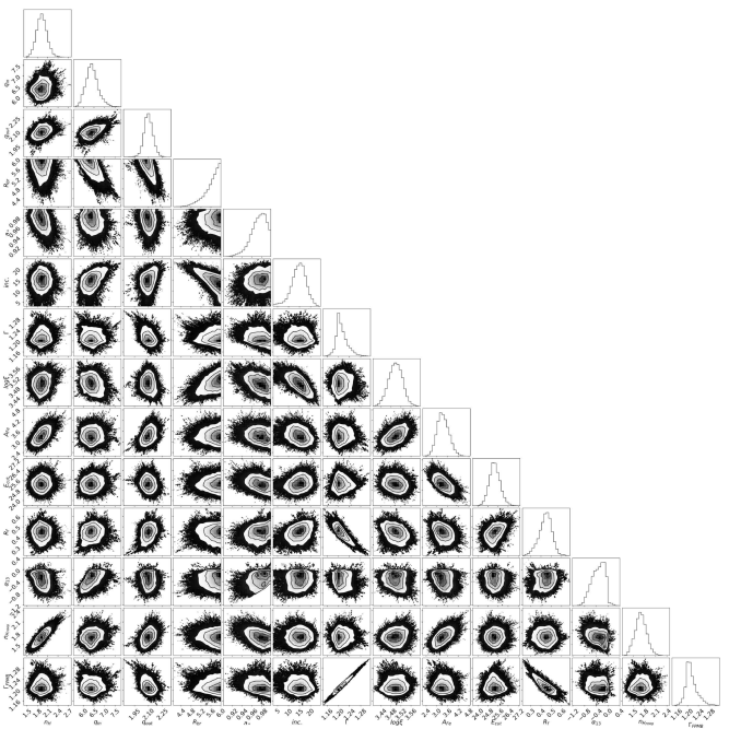
Figure 6.— As in Fig. 4 for GRS 1739–278.

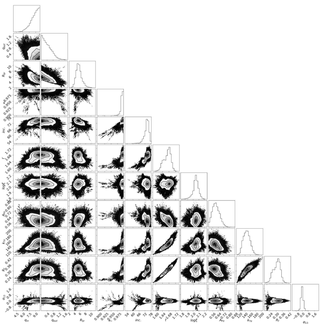
Figure 7.— As in Fig. 4 for GS 1354–645.

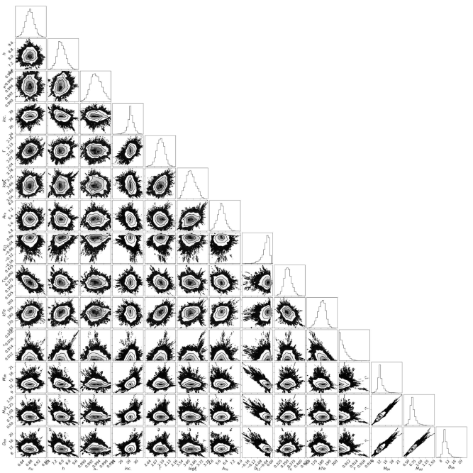
Figure 8.— As in Fig. 4 for GX 339–4.

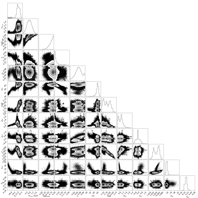
Figure 9.— As in Fig. 4 for Swift J1658.2–4242.

Figure 10.— Histogram of the Johannsen deformation parameter $\alpha_{13}$ resulting from the combination of the measurements from the six sources analyzed in this work. The red solid line marks the estimate of $\alpha_{13}$ and the dashed, dashed-dotted, and dotted lines mark, respectively, the 1-, 2-, and 3-$\sigma$ limits.

	4U 1630–472	EXO 1846–031	GRS 1739–278	GS 1354–645	GX 339–4	Swift J1658.2–4242
xillver
$\chi^{2}_{\nu}$	2609.14/1104	2856.58/2599	1453.92/1118	3116.80/2725	1521.35/649	1858.85/1650
	=2.363	=1.099	=1.300	=1.144	=2.344	=1.126
relxill(Cp)_nk
$\alpha_{13}$	$0.16_{-0.31}^{+0.31}$	$-0.03_{-0.18}^{+0.17}$	$-0.31_{-0.53}^{+0.64}$	$-0.04_{-0.87}^{+0.58}$	$-0.010_{-0.104}^{+0.066}$	$-0.03_{-0.39}^{+0.19}$
$\chi^{2}_{\nu}$	1273.74/1082	2751.90/2594	1283.78/1112	2895.07/2720	874.22/645	1754.14/1642
	=1.177	=1.061	=1.154	=1.065	=1.355	=1.068
relxilllp(Cp)_nk
$\alpha_{13}$	$-0.03_{-0.18}^{+0.63}$	$2.7_{-3.9}^{+1.8}$	$0.4_{-4.9}^{+4.1}$	$0.4_{-1.9}^{+2.1}$	$-0.023_{-0.030}^{+0.137}$	$-0.05_{-0.97}^{+1.21}$
$\chi^{2}_{\nu}$	1224.01/1084	2773.72/2596	1326.45/1114	2936.96/2722	869.15/647	1741.81/1644
	=1.129	=1.068	=1.190	=1.079	=1.346	=1.059

Table 5Summary of $\chi^{2}$s and 3-$\sigma$ measurements of $\alpha_{13}$ modeling the reflection component with xillver, relxill(Cp)_nk, and relxilllp(Cp)_nk.

3.2.2 Combined measurement

If we assume that the value of $\alpha_{13}$ is the same for all black holes, we can combine the six individual measurements to get a joint measurement. Such a possibility would depend on the (unknown) underlying theory. Within the phenomenological framework of the Johannsen metric, it is just an assumption. If astrophysical black holes had more “hairs” than those predicted by General Relativity (e.g. some extra charge), deviations from the Kerr background would be different for every object. In such a case, we should not combine the data to get a joint measurement of $\alpha_{13}$. If some form of the no-hair theorems would still hold in Nature, all astrophysical black holes may share the same deviation from the Kerr solution and the deformation parameter may have the same value for all sources (or very similar value for all sources of the same class, like stellar-mass black holes). In this section, we thus assume this second scenario.

There are also different methods to combine the individual measurements to get a joint measurement of the deformation parameter $\alpha_{13}$. Here we combine the distribution of the six measurements and we get the histogram in Fig. 10. The 1-$\sigma$ joint measurement is

$$\alpha_{13}=-0.04_{-0.21}^{+0.06}\,.$$ (1)

The 3-$\sigma$ measurement is $\alpha_{13}=-0.04_{-0.90}^{+0.93}$.

4. Discussion and conclusions

In our study, we employed state-of-the-art in relativistic reflection modeling to analyze the currently available best X-ray data of reflection dominated spectra of black hole binaries to obtain precise and accurate constraints on the Kerr black hole hypothesis. Our results turn out to be in perfect agreement with the predictions of General Relativity and are summarized in Fig. 11, where we show the 3-$\sigma$ measurements of $\alpha_{13}$ for every source.

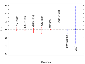
Figure 11.— Summary of the 3-$\sigma$ measurements on the Johannsen deformation parameter $\alpha_{13}$ from the six sources analyzed in this work. We also show the 3-$\sigma$ constraint from GW170608 (Cárdenas-Avendaño et al., 2020) and the 1-$\sigma$ constraint from M87^∗ (Psaltis et al., 2020).

Our constraints are much stronger than that recently obtained from the 2017 observations of the Event Horizon Telescope of the supermassive black holes in the galaxy M87, which is $-3.6<\alpha_{13}<5.9$ at 1-$\sigma$ (Psaltis et al., 2020). Employing the Einstein Equations for the production of gravitational waves, it is possible to constrain $\alpha_{13}$ from the LIGO/Virgo data (Cárdenas-Avendaño et al., 2020). The strongest constraint was obtained from GW170608 and the 3-$\sigma$ measurement is $\alpha_{13}=-0.11\pm 0.79$, which is shown together with our constraints from NuSTAR data in Fig. 11. The constraints obtained here are at worst comparable with the strongest constraint obtained from gravitational waves. For some sources (GX 339–4 and EXO 1846–031), our constraints are much stronger.

We note that the constraints obtained with our technique strongly depend on the specific source and observation, because the morphology of the accretion material and the spectrum of the source can significantly change from source to source and even for the same source from an outburst to another outburst. Gravitational wave tests are less sensitive to the specific event because, in any case, every event is the coalescence of two black holes and effects of the surrounding environment are normally negligible.

To clarify the significance of a relativistic reflection component (again a non-relativistic reflection component that could be modeled by xillver), as well as the impact of the emissivity profile (i.e., broken power-law vs lamppost geometry), in Tab. 5 we show $\chi^{2}$ and measurement of $\alpha_{13}$ for different fits. For all spectra, xillver does not provide an acceptable fit. When we employ a relativistic reflection component, we choose the model providing the lowest $\chi^{2}$ as the best model. We note that, when the best model is relxilllp(Cp)_nk (lamppost geometry), the model with a broken power-law does not provide a too bad fit and the measurement of $\alpha_{13}$ is consistent with that obtained with the lamppost model. The contrary is not true: if the best model is relxill(Cp)_nk (broken power-law emissivity profile), the model with a lamppost geometry cannot constrain the deformation parameter well. Such a result is perfectly understandable: the broken power-law can approximate well the lamppost profile, while the latter may not approximate well the broken power-law. For the sources fit with a broken power-law (EXO 1846–031, GRS 1739–278, and GS 1354–645), we find $q_{\rm out}$ quite low, while at large radii the profile of the lamppost model is similar to a power-law emissivity profile with emissivity index close to 3.

The models employed in our study to fit the spectra of the six sources present a number of simplifications that could, potentially, introduce undesirable systematic uncertainties to make our constraints on the Johannsen deformation parameter $\alpha_{13}$ unreliable. Here we point out that the main systematic uncertainties are well under control for these specific sources.

1. Inner edge of the accretion disk. In our measurements of the Johannsen deformation parameter $\alpha_{13}$ reported in this work, we assume that the inner edge of the accretion disk is at the ISCO radius. While there is a common consensus that this is a good approximation for sources in the soft state with an Eddington-scaled disk luminosity between $\sim$5% to $\sim$30% (Steiner et al., 2010; Kulkarni et al., 2011), the issue is more controversial for sources in the hard state and the disk may be truncated at a larger radius. We note, however, that this assumption has a negligible impact on our measurements of $\alpha_{13}$ because, assuming $R_{\rm in}=R_{\rm ISCO}$, we find that all our sources are very-fast-rotating black holes, with a value of the spin parameter $a_{*}$ close to the maximum limit. The inner edges of the accretion disks of these sources is very close to the black hole. Fitting the data with $R_{\rm in}$ as a free parameter, we recover the same results.

2. Thickness of the disk. The versions of relxill_nk and nkbb employed in our analysis assume that the accretion disk is infinitesimally thin, while in reality the disk has a finite thickness, which increases as the mass accretion rate increases. Reflection and thermal models with accretion disks of finite thickness were presented in Taylor & Reynolds (2018); Abdikamalov et al. (2020); Zhou et al. (2020) and their impact on the estimate of the model parameters was explored. Again, since we found that our sources have a spin parameter close to the maximum limit, the radiative efficiency is very high and the actual thickness of the disk is modest. In such a case, the impact on the constraints on $\alpha_{13}$ is negligible, as it was explicitly shown in Abdikamalov et al. (2020).

3. Radiation from the plunging region. In our model to fit the data, we ignore the radiation emitted from the plunging region. If the Eddington-scaled mass accretion rate is not very low, below 1% for fast-rotating black holes, the plunging region is optically thick (Reynolds & Begelman, 1997). In such a case, the Comptonized photons from the corona should generate a reflection component. However, the gas is highly ionized in the plunging region (Reynolds & Begelman, 1997; Wilkins et al., 2020). The impact of such radiation on the estimate of the Johannsen deformation parameter $\alpha_{13}$ was studied in Cárdenas-Avendaño et al. (2020), where it was shown that for fast-rotating black holes associated with very small plunging regions (which is the case of the sources presented in our study) the impact is negligible for present and near future X-ray data.

4. Disk emissivity profile. The emissivity profile of the accretion disk is an important ingredient to properly model the reflection spectrum of the source and an incorrect emissivity profile can lead to a non-vanishing deformation parameter $\alpha_{13}$ (Zhang et al., 2019). In our study, we tried power law, broken power law, and lamppost model, and eventually we selected the emissivity profile providing the best fit. As we have already discussed, when the best model is the lamppost geometry, the measurement with the broken power-law model is not too different, as the the latter is a more flexible profile and can approximate the lamppost one well. The contrary is not true, and if the spectrum prefers a broken power-law, the fit and the constraints with the lamppost model may be bad.

5. Disk electron density. We fit the data assuming a disk electron density $n_{\rm e}=10^{15}$ cm^-3, which is the default value in relxil_nk. However, such a value is likely too low for the accretion disk of stellar-mass black holes with a relatively high mass accretion rate, which is the case of our sources (Jiang et al., 2019a, b). The impact of the disk electron density on the estimate of $\alpha_{13}$ was explored in previous studies (Tripathi et al., 2021; Zhang et al., 2019), where we did not find any clear bias in the constraint on $\alpha_{13}$ from the value of $n_{\rm e}$, which is consistent with the conclusion in Jiang et al. (2019a, b) that underestimating the disk electron density has no significant impact on the estimate of the black hole spin (assuming the Kerr metric).

6. Returning radiation. Because of the strong light bending near the black hole, reflection radiation emitted from the accretion disk may return to the accretion disk and be reflected again. Since the reflection spectrum depends on the incident one, the reflection radiation returning to the disk cannot be reabsorbed in the emissivity profile induced by the corona. At the moment, there are only some preliminary and incomplete studies on the impact of the returning radiation on the estimate of the model parameters when the effect is not included in the calculations. The effect is more important for sources with the inner edge of the accretion disk very close to the black hole, which is the case for our sources. While we admit that the systematic uncertainties of such an effect is not well under control as of now, we note that it is important for low inclination angles and quite small for edge-on disks (Riaz et al., 2020). In other words, we do not expect that the returning radiation has any relevant impact on our analysis of EXO 1846–031, GS 1354–645, and Swift J1658–4242, while we are currently unable to quantify the impact on the constraint on $\alpha_{13}$ for 4U 1630–472, GRS 1739–278, and GX 339–4.

Last, we wish to point out that our constraints can be improved with the next generation of X-ray observatories. eXTP (Zhang et al., 2016) will provide simultaneous timing, spectral, and polarization measurements of the disk reflection component. Athena (Nandra et al., 2013) will have a much better energy resolution near the iron line.

Acknowledgments – We thank Alejandro Cardenas-Avendano for useful discussions about the constraints from the LIGO/Virgo data. This work was supported by the Innovation Program of the Shanghai Municipal Education Commission, Grant No. 2019-01-07-00-07-E00035, the National Natural Science Foundation of China (NSFC), Grant No. 11973019, and Fudan University, Grant No. JIH1512604. Y.Z. acknowledges the support from China Scholarship Council (CSC 201906100030). D.A. is supported through the Teach@Tübingen Fellowship. J.J. acknowledges the support from Tsinghua Shuimu Scholar Program and Tsinghua Astrophysics Outstanding Fellowship. A.T., C.B., J.J., and H.L. are members of the International Team 458 at the International Space Science Institute (ISSI), Bern, Switzerland, and acknowledge support from ISSI during the meetings in Bern.

Appendix A A. Johannsen metric

For the convenience of the readers, we report here the expression of the Johannsen metric, but more details can be found in the original paper (Johannsen, 2013). In Boyer-Lindquist-like coordinates, the line element is

$$ds^{2} = -\frac{\tilde{\Sigma}\left(\Delta-a^{2}A_{2}^{2}\sin^{2}\theta\right)}{B^{2}}dt^{2}+\frac{\tilde{\Sigma}}{\Delta A_{5}}dr^{2}+\tilde{\Sigma}d\theta^{2}$$ (A1)

$$-\frac{2a\left[\left(r^{2}+a^{2}\right)A_{1}A_{2}-\Delta\right]\tilde{\Sigma}\sin^{2}\theta}{B^{2}}dtd\phi+\frac{\left[\left(r^{2}+a^{2}\right)^{2}A_{1}^{2}-a^{2}\Delta\sin^{2}\theta\right]\tilde{\Sigma}\sin^{2}\theta}{B^{2}}d\phi^{2}\,,$$

where $M$ is the black hole mass, $a=J/M$, $J$ is the black hole spin angular momentum, $\tilde{\Sigma}=\Sigma+f$, and

$$\Sigma=r^{2}+a^{2}\cos^{2}\theta\,,\qquad\Delta=r^{2}-2Mr+a^{2}\,,\qquad B=\left(r^{2}+a^{2}\right)A_{1}-a^{2}A_{2}\sin^{2}\theta\,.$$ (A2)

The functions $f$, $A_{1}$, $A_{2}$, and $A_{5}$ are defined as

$$f=\sum^{\infty}_{n=3}\epsilon_{n}\frac{M^{n}}{r^{n-2}}\,,\quad A_{1}=1+\sum^{\infty}_{n=3}\alpha_{1n}\left(\frac{M}{r}\right)^{n}\,,\quad A_{2}=1+\sum^{\infty}_{n=2}\alpha_{2n}\left(\frac{M}{r}\right)^{n}\,,\quad A_{5}=1+\sum^{\infty}_{n=2}\alpha_{5n}\left(\frac{M}{r}\right)^{n}\,,$$ (A3)

where $\{\epsilon_{n}\}$, $\{\alpha_{1n}\}$, $\{\alpha_{2n}\}$, and $\{\alpha_{5n}\}$ are four infinite sets of deformation parameters without constraints from the Newtonian limit and Solar System experiments. In the present study, we have only considered the deformation parameter $\alpha_{13}$, which has the strongest impact on the reflection spectrum. All other deformation parameters are set to zero.

We remind the readers that the Johannsen metric is a phenomenological deformation from the Kerr solution, and specifically designed for testing the Kerr black hole hypothesis with electromagnetic data. There is no theory from which the metric is derived, so no a priori indications about the value of these deformation parameters. The metric is obtained by imposing that the spacetime is regular outside of the event horizon (no naked singularities, closed time-like curves, etc.) and has a Carter-like constant (i.e., the equations of motion of a test-particle can be written in first-order form). Under these conditions, we get a metric characterized by four free functions ($f$, $A_{1}$, $A_{2}$, and $A_{5}$), which are then written in the form shown in Eq. (A3). The impact of the deformation parameters $\epsilon_{3}$, $\alpha_{13}$, $\alpha_{22}$, and $\alpha_{52}$ on a narrow line was shown in Bambi et al. (2017). Higher order deformation parameters (i.e. $\epsilon_{n}$ with $n\geq 4$, $\alpha_{1n}$ with $n\geq 4$, etc.) have a qualitatively very similar impact on a narrow line and on the full reflection spectrum. Our choice of considering only the deformation parameter $\alpha_{13}$ can thus be seen as a proof of concept of our current capabilities and our results should not be generalized to any generic deformation from the Kerr background.

Appendix B B. The relxill_nk package

relxill_nk (Bambi et al., 2017; Abdikamalov et al., 2019) is an extension of the relxill package (Dauser et al., 2013; García et al., 2014) to non-Kerr spacetimes. The default flavor is relxill_nk, but in the spectral analysis of our work we have also used relxilllp_nk, relxillCp_nk, and relxilllpCp_nk.

The spacetime metric is described by the black hole spin parameter $a_{*}$ and by the Johannsen deformation parameter $\alpha_{13}$, while the black hole mass does not directly enter the calculations of the reflection spectrum. The position of the observer is specified by the inclination angle of the disk with respect to the line of sight of the observer, $i$. In the default flavor relxill_nk, there are no assumptions about the coronal geometry and thus the emissivity profile of the disk is modeled with a broken power-law with three parameters: inner emissivity index $q_{\rm in}$, outer emissivity index $q_{\rm out}$, and breaking radius $R_{\rm br}$. In the lamppost version of the model (the flavors with lp), we assume a lamppost coronal geometry: the corona is a point-like and isotropic source along the black hole spin axis and we have only one parameter, the coronal height $h$. In all flavors, the material of the accretion disk is characterized by the ionization parameter $\xi$ (measured in erg cm s^-1) and the iron abundance $A_{\rm Fe}$ (measured in units of solar iron abundance). In the default flavor relxill_nk, the coronal spectrum is described by a power-law with a high-energy cutoff and we have thus two parameters: the photon index $\Gamma$ and the high-energy cutoff $E_{\rm cut}$. The Cp flavors of the model employ the nthComp model for the description of the coronal spectrum and the high-energy cutoff $E_{\rm cut}$ is replaced by the coronal temperature $kT_{\rm e}$. The reflection fraction, $R_{\rm f}$, is the relative normalization between the reflection spectrum from the disk and the spectrum of the corona. The latter can be omitted (as in our spectral analysis of GX 339–4 and Swift J1658.2–4242), and in such a case the radiation from the corona is described by an external model.

References

- Abbott et al. (2016) Abbott, B. P., Abbott, R., Abbott, T. D., et al. 2016, Phys. Rev. Lett., 116, 221101. doi:10.1103/PhysRevLett.116.221101
- Abbott et al. (2019) Abbott, B. P., Abbott, R., Abbott, T. D., et al. 2019, Phys. Rev. D, 100, 104036. doi:10.1103/PhysRevD.100.104036
- Abdikamalov et al. (2019) Abdikamalov, A. B., Ayzenberg, D., Bambi, C., et al. 2019, ApJ, 878, 91. doi:10.3847/1538-4357/ab1f89
- Abdikamalov et al. (2020) Abdikamalov, A. B., Ayzenberg, D., Bambi, C., et al. 2020, ApJ, 899, 80. doi:10.3847/1538-4357/aba625
- Bambi (2017) Bambi, C. 2017, Reviews of Modern Physics, 89, 025001. doi:10.1103/RevModPhys.89.025001
- Bambi (2018) Bambi, C. 2018, Annalen der Physik, 530, 1700430. doi:10.1002/andp.201700430
- Bambi et al. (2020) Bambi, C., Brenneman, L. W., Dauser, T., et al. 2020, arXiv:2011.04792
- Bambi et al. (2017) Bambi, C., Cárdenas-Avendaño, A., Dauser, T., et al. 2017, ApJ, 842, 76. doi:10.3847/1538-4357/aa74c0
- Bambi et al. (2014) Bambi, C., Malafarina, D., & Tsukamoto, N. 2014, Phys. Rev. D, 89, 127302. doi:10.1103/PhysRevD.89.127302
- Cao et al. (2018) Cao, Z., Nampalliwar, S., Bambi, C., et al. 2018, Phys. Rev. Lett., 120, 051101. doi:10.1103/PhysRevLett.120.051101
- Cárdenas-Avendaño et al. (2020) Cárdenas-Avendaño, A., Nampalliwar, S., & Yunes, N. 2020, Classical and Quantum Gravity, 37, 135008. doi:10.1088/1361-6382/ab8f64
- Cárdenas-Avendaño et al. (2020) Cárdenas-Avendaño, A., Zhou, M., & Bambi, C. 2020, Phys. Rev. D, 101, 123014. doi:10.1103/PhysRevD.101.123014
- Chruściel et al. (2012) Chruściel, P. T., Costa, J. L., & Heusler, M. 2012, Living Reviews in Relativity, 15, 7. doi:10.12942/lrr-2012-7
- Dauser et al. (2013) Dauser, T., Garcia, J., Wilms, J., et al. 2013, MNRAS, 430, 1694. doi:10.1093/mnras/sts710
- Draghis et al. (2020) Draghis, P. A., Miller, J. M., Cackett, E. M., et al. 2020, ApJ, 900, 78. doi:10.3847/1538-4357/aba2ec
- Einstein (1916) Einstein, A. 1916, Annalen der Physik, 354, 769. doi:10.1002/andp.19163540702
- El-Batal et al. (2016) El-Batal, A. M., Miller, J. M., Reynolds, M. T., et al. 2016, ApJ, 826, L12. doi:10.3847/2041-8205/826/1/L12
- García et al. (2014) García, J., Dauser, T., Lohfink, A., et al. 2014, ApJ, 782, 76. doi:10.1088/0004-637X/782/2/76
- García & Kallman (2010) García, J. & Kallman, T. R. 2010, ApJ, 718, 695. doi:10.1088/0004-637X/718/2/695
- Giddings (2017) Giddings, S. B. 2017, Nature Astronomy, 1, 0067. doi:10.1038/s41550-017-0067
- Harrison et al. (2013) Harrison, F. A., Craig, W. W., Christensen, F. E., et al. 2013, ApJ, 770, 103. doi:10.1088/0004-637X/770/2/103
- Herdeiro & Radu (2014) Herdeiro, C. A. R. & Radu, E. 2014, Phys. Rev. Lett., 112, 221101. doi:10.1103/PhysRevLett.112.221101
- Jiang et al. (2019a) Jiang, J., Fabian, A. C., Wang, J., et al. 2019a, MNRAS, 484, 1972. doi:10.1093/mnras/stz095
- Jiang et al. (2019b) Jiang, J., Fabian, A. C., Dauser, T., et al. 2019b, MNRAS, 489, 3436. doi:10.1093/mnras/stz2326
- Jiang et al. (2020) Jiang, J., Fürst, F., Walton, D. J., et al. 2020, MNRAS, 492, 1947. doi:10.1093/mnras/staa017
- Johannsen (2013) Johannsen, T. 2013, Phys. Rev. D, 88, 044002. doi:10.1103/PhysRevD.88.044002
- Kerr (1963) Kerr, R. P. 1963, Phys. Rev. Lett., 11, 237. doi:10.1103/PhysRevLett.11.237
- Kleihaus et al. (2011) Kleihaus, B., Kunz, J., & Radu, E. 2011, Phys. Rev. Lett., 106, 151104. doi:10.1103/PhysRevLett.106.151104
- King et al. (2014) King, A. L., Walton, D. J., Miller, J. M., et al. 2014, ApJ, 784, L2. doi:10.1088/2041-8205/784/1/L2
- Kulkarni et al. (2011) Kulkarni, A. K., Penna, R. F., Shcherbakov, R. V., et al. 2011, MNRAS, 414, 1183. doi:10.1111/j.1365-2966.2011.18446.x
- Miller et al. (2013) Miller, J. M., Parker, M. L., Fuerst, F., et al. 2013, ApJ, 775, L45. doi:10.1088/2041-8205/775/2/L45
- Miller et al. (2015) Miller, J. M., Tomsick, J. A., Bachetti, M., et al. 2015, ApJ, 799, L6. doi:10.1088/2041-8205/799/1/L6
- Mori et al. (2019) Mori, K., Hailey, C. J., Mandel, S., et al. 2019, ApJ, 885, 142. doi:10.3847/1538-4357/ab4b47
- Nandra et al. (2013) Nandra, K., Barret, D., Barcons, X., et al. 2013, arXiv:1306.2307
- Parker et al. (2016) Parker, M. L., Tomsick, J. A., Kennea, J. A., et al. 2016, ApJ, 821, L6. doi:10.3847/2041-8205/821/1/L6
- Parker et al. (2015) Parker, M. L., Tomsick, J. A., Miller, J. M., et al. 2015, ApJ, 808, 9. doi:10.1088/0004-637X/808/1/9
- Psaltis et al. (2020) Psaltis, D., Medeiros, L., Christian, P., et al. 2020, Phys. Rev. Lett., 125, 141104. doi:10.1103/PhysRevLett.125.141104
- Psaltis et al. (2008) Psaltis, D., Perrodin, D., Dienes, K. R., et al. 2008, Phys. Rev. Lett., 100, 091101. doi:10.1103/PhysRevLett.100.091101
- Reynolds (2019) Reynolds, C. S. 2019, Nature Astronomy, 3, 41. doi:10.1038/s41550-018-0665-z
- Reynolds & Begelman (1997) Reynolds, C. S. & Begelman, M. C. 1997, ApJ, 488, 109. doi:10.1086/304703
- Riaz et al. (2020) Riaz, S., Szanecki, M., Niedźwiecki, A., et al. 2021, ApJ, 910, 49. doi:10.3847/1538-4357/abe2a3
- Ross & Fabian (2005) Ross, R. R. & Fabian, A. C. 2005, MNRAS, 358, 211. doi:10.1111/j.1365-2966.2005.08797.x
- Steiner et al. (2010) Steiner, J. F., McClintock, J. E., Remillard, R. A., et al. 2010, ApJ, 718, L117. doi:10.1088/2041-8205/718/2/L117
- Tao et al. (2019) Tao, L., Tomsick, J. A., Qu, J., et al. 2019, ApJ, 887, 184. doi:10.3847/1538-4357/ab5282
- Taylor & Reynolds (2018) Taylor, C. & Reynolds, C. S. 2018, ApJ, 868, 109. doi:10.3847/1538-4357/aae9f2
- Tomsick et al. (2014) Tomsick, J. A., Nowak, M. A., Parker, M., et al. 2014, ApJ, 780, 78. doi:10.1088/0004-637X/780/1/78
- Tripathi et al. (2021) Tripathi, A., Abdikamalov, A. B., Ayzenberg, D., et al. 2021, ApJ, 907, 31. doi:10.3847/1538-4357/abccbd
- Tripathi et al. (2019) Tripathi, A., Nampalliwar, S., Abdikamalov, A. B., et al. 2019, ApJ, 875, 56. doi:10.3847/1538-4357/ab0e7e
- Tripathi et al. (2020) Tripathi, A., Zhou, M., Abdikamalov, A. B., et al. 2020, ApJ, 897, 84. doi:10.3847/1538-4357/ab9600
- Walton et al. (2017) Walton, D. J., Mooley, K., King, A. L., et al. 2017, ApJ, 839, 110. doi:10.3847/1538-4357/aa67e8
- Walton et al. (2016) Walton, D. J., Tomsick, J. A., Madsen, K. K., et al. 2016, ApJ, 826, 87. doi:10.3847/0004-637X/826/1/87
- Wilkins et al. (2020) Wilkins, D. R., Reynolds, C. S., & Fabian, A. C. 2020, MNRAS, 493, 5532. doi:10.1093/mnras/staa628
- Will (2014) Will, C. M. 2014, Living Reviews in Relativity, 17, 4. doi:10.12942/lrr-2014-4
- Xu et al. (2018a) Xu, Y., Harrison, F. A., García, J. A., et al. 2018a, ApJ, 852, L34. doi:10.3847/2041-8213/aaa4b2
- Xu et al. (2018b) Xu, Y., Harrison, F. A., Kennea, J. A., et al. 2018b, ApJ, 865, 18. doi:10.3847/1538-4357/aada03
- Xu et al. (2020) Xu, Y., Harrison, F. A., Tomsick, J. A., et al. 2020, ApJ, 893, 30. doi:10.3847/1538-4357/ab7dc0
- Xu et al. (2018c) Xu, Y., Nampalliwar, S., Abdikamalov, A. B., et al. 2018c, ApJ, 865, 134. doi:10.3847/1538-4357/aadb9d
- Yagi & Stein (2016) Yagi, K. & Stein, L. C. 2016, Classical and Quantum Gravity, 33, 054001. doi:10.1088/0264-9381/33/5/054001
- Yunes et al. (2016) Yunes, N., Yagi, K., & Pretorius, F. 2016, Phys. Rev. D, 94, 084002. doi:10.1103/PhysRevD.94.084002
- Zhang et al. (2016) Zhang, S. N., Feroci, M., Santangelo, A., et al. 2016, Proc. SPIE, 9905, 99051Q. doi:10.1117/12.2232034
- Zhang et al. (2019) Zhang, Y., Abdikamalov, A. B., Ayzenberg, D., et al. 2019, ApJ, 884, 147. doi:10.3847/1538-4357/ab4271
- Zhou et al. (2019) Zhou, M., Abdikamalov, A. B., Ayzenberg, D., et al. 2019, Phys. Rev. D, 99, 104031. doi:10.1103/PhysRevD.99.104031
- Zhou et al. (2020) Zhou, M., Abdikamalov, A. B., Ayzenberg, D., et al. 2020, MNRAS, 496, 497. doi:10.1093/mnras/staa1591