Dynamic Traffic Modeling from Overhead Imagery

Abstract

Our goal is to use overhead imagery to understand patterns in traffic flow, for instance answering questions such as how fast could you traverse Times Square at 3am on a Sunday. A traditional approach for solving this problem would be to model the speed of each road segment as a function of time. However, this strategy is limited in that a significant amount of data must first be collected before a model can be used and it fails to generalize to new areas. Instead, we propose an automatic approach for generating dynamic maps of traffic speeds using convolutional neural networks. Our method operates on overhead imagery, is conditioned on location and time, and outputs a local motion model that captures likely directions of travel and corresponding travel speeds. To train our model, we take advantage of historical traffic data collected from New York City. Experimental results demonstrate that our method can be applied to generate accurate city-scale traffic models.

1 Introduction

Road transportation networks have become extremely large and complex. According to the Bureau of Transportation Statistics [31], there are approximately 6.6 million kilometers of roads in the United States alone. For most individuals, navigating these complex road networks is a daily challenge. A recent study found that the average driver in the U.S. travels approximately $17\,500$ kilometers per year in their vehicle, which equates to more than 290 hours behind the wheel [33].

As such, traffic modeling and analysis has become an increasingly important topic for urban development and planning. The Texas A&M Transportation Institute [26] estimated that in 2017, considering 494 U.S. urban areas, there were 8.8 billion vehicle-hours of delay and 12.5 billion liters of wasted fuel, resulting in a congestion cost of 179 billion dollars. Given these far-reaching implications, there is significant interest in understanding traffic flow and developing new methods to counteract congestion.

Figure 1: Using our approach to dynamically model traffic flow in The Bronx, New York City. (left) Predicted traffic speeds for Monday at 4am and (right) Monday at 8am. Green (red) corresponds to faster (slower).

Numerous cities are starting to equip themselves with intelligent transportation systems, such as adaptive traffic control, that take advantage of recent advances in computer vision and machine learning. For example, Pittsburgh recently deployed smart traffic signals at fifty intersections that use artificial intelligence to estimate traffic volume and optimize traffic flow in real-time. An initial pilot study [27] indicated travel times were reduced by 25%, time spent waiting at signals by 40%, number of stops by 30%, and emissions by 20%. Ultimately, interest in applying machine learning to problems in traffic management continues to grow due to its potential for improving safety, decreasing congestion, and reducing emissions.

Figure 2: In urban environments, traffic speeds change drastically throughout the day. For example, traffic congestion in downtown Cincinnati during the (left) early morning (12am to 7am) is minimal compared to (right) afternoon peak (4pm to 7pm) on a weekday (visualization from [1]). Speeds are shown as percent from free-flow where green (red) is faster (slower).

Direct access to empirical traffic data is useful for planners to analyze congestion in relation to the underlying street network, as well as for validating models and guiding infrastructure investments. Unfortunately, historical information relating time, traffic speeds, and street networks has typically been expensive to acquire and limited to only primary roads. Only very recently has a large corpus of traffic speed data been released to the public. In May of 2019, Uber Technologies, Inc. (an American multinational ridesharing company) announced Uber Movement Speeds [1], a dataset of street speeds collected from drivers of their ridesharing platform. However, even this data has limitations, including: 1) coverage, speed data is only available for 5 large metropolitan cities at the time of release and 2) granularity, not all roads are traversed at all times (or traversed at all). For example, only $29\%$ of road segments in New York City have historical traffic data for Monday at 12pm, considering every Monday in 2018.

In this work, our goal is to use historical traffic speeds to build a complete model of traffic flow for a given city (Figure 2). Traditional approaches for modeling traffic flow assume that the road network is known (i.e., in the form of a graph reflecting the presence and connectivity of road segments) and model road segments individually. However, this approach is limited in that it cannot generalize to new areas and it gives noisy estimates for road segments with few samples. Instead, we explore how image-driven mapping can be applied to model traffic flow directly from overhead imagery. We envision that such a model could be used by urban planners to understand city-scale traffic patterns when the complete road network is unknown or insufficient empirical traffic data is available.

We propose an automatic approach for generating dynamic maps of traffic speeds using convolutional neural networks (CNNs). We frame this as a multi-task learning problem, and design a network architecture that simultaneously learns to segment roads, estimate orientation, and predict traffic speeds. Along with overhead imagery, the network takes as input contextual information describing the location and time. Ultimately, the output of our method can be considered as a local motion model that captures likely directions of travel and corresponding travel speeds. To support training and evaluating our methods, we introduce a new dataset that takes advantage of a year of traffic speeds for New York City, collected from Uber Movement Speeds.

Extensive experiments show that our approach is able to capture complex relationships between the underlying road infrastructure and traffic flow, enabling understanding of city-scale traffic patterns, without requiring the road network to be known in advance. This enables our approach to generalize to new areas. The main contributions of this work are summarized as follows:

• introducing a new dataset for fine-grained road understanding,

• proposing a multi-task CNN architecture for estimating a localized motion model directly from an overhead image,

• integrating location and time metadata to enable dynamic traffic modeling,

• an extensive quantitative and qualitative analysis, including generating dynamic city-scale travel-time maps.

Our approach has several potential real-world applications, including forecasting traffic speeds and providing estimates of historical traffic speeds on roads which were not traversed during a specific time period.

2 Related Work

The field of urban planning [15] seeks to understand urban environments and how they are used in order to guide future decision making. The overarching goal is to shape the pattern of growth as a community expands to achieve a desirable land-use pattern. A major factor here is understanding how the environment influences human activity. For example, research has shown how the physical environment is associated with physical activity (walking/cycling) and subsequently impacts health [24].

Transportation planning is a specific subarea of urban planning that focuses on the design of transportation systems. The goal is to develop systems of travel that align with and promote a desired policy of human activity [19]. Decisions might include how and where to place roads, sidewalks, and other infrastructure to minimize congestion. As such, decades of research has focused on understanding traffic flow, i.e., the interactions of travelers and the underlying infrastructure. For example, Krauß [14] proposes a model of microscopic traffic flow to understand different types of traffic congestion. Meanwhile other work focuses on simulating urban mobility [13].

In computer vision, relevant work seeks to infer properties of the local environment directly from imagery. For example estimating physical attributes like land cover and land use [23, 37], categorizing the type of scene [41], and relating appearance to location [35, 36, 25]. Other work focuses on understanding urban environments. Albert et al. [4] analyze and compare urban environments at the scale of cities using satellite imagery. Dubey et al. [8] explore the relationship between the appearance of the physical environment and the urban perception of its residents by predicting perceptual attributes such as safe and beautiful.

Specific to urban transportation, many studies have explored how to identify roads and infer road networks directly from overhead imagery [20, 18, 17, 5, 32]. Recent methods in this area take advantage of convolutional neural networks for segmenting an overhead image, then generate a graph topology directly from the segmentation output. Mapping roads is an important problem as it can positively impact local communities as well as support disaster response [21, 28]. However, identifying roads is just the first step. Other work has focused on estimating properties of roads, including safety [30].

Understanding how roads are used, in particular traffic speeds, is important for studying driver behavior, improving safety, decreasing collisions, and aiding infrastructure planning. Therefore, several works have tackled the problem of estimating traffic speeds from imagery. Hua et al. [11] detect, track, and estimate traffic speeds for vehicles in traffic videos. Song et al. [29] estimate the free-flow speed of a road segment from a co-located overhead image and corresponding road metadata. Van Etten [9] segments roads and estimates road speed limits. Unlike this previous work, our goal is to dynamically model traffic flow over time.

Similarly, traffic forecasting is an important research area. Abadi et al. [3] propose an autoregressive model for predicting the flows of a traffic network and demonstrate the ability to forecast near-term future traffic flows. Zhang et al. [38] predict crowd flows between subregions of a city based on historical trajectory data, weather, and events. Wang et al. [34] propose a deep learning framework for path-based travel time estimation. These methods typically assume prior knowledge of the spatial connectivity of the road network, unlike our work which operates directly on overhead imagery.

3 A Large Traffic Speeds Dataset

Figure 3: Example traffic speed data from Uber Movement Speeds for New York City (visualized as free-flow speeds for January 2018).

To support training and evaluating our methods, we introduce the Dynamic Traffic Speeds (DTS) dataset that takes advantage of a year of historical traffic speeds for New York City. Our traffic speed data is collected from Uber Movement Speeds [1], a dataset of publicly available aggregated speed data over road segments at hourly frequencies.

3.1 Uber Movement Speeds

During rideshare trips, Uber (via their Uber Driver application) frequently collects GPS data including latitude, longitude, speed, direction, and time. While this data supports many functionalities, it is also stored for offline processing, where it is aggregated and used to derive speed data. Additionally, Uber uses OpenStreetMap as the source of their underlying map data (i.e., road network).

Given the map and GPS data as input, an extensive process is used to 1) match the GPS data to locations on the street network, 2) compute segment traversal speeds using the matched data, and 3) aggregate speeds along each segment. Please refer to the whitepaper [2] for a detailed overview of this process. Ultimately, the publicly released data includes the road segment identifier and average speed along that segment at an hourly resolution. Note that bidirectional roads, represented as line strings, are twinned and a speed estimate is provided for each direction.

3.2 Augmenting with Overhead Imagery

To support our methods, we generated an aligned dataset of overhead images, contained road segments, and historical traffic speeds. We started by collecting road geometries and speed data from Uber Movement Speeds for New York City during the 2018 calendar year. This resulted in over 292 million records, or approximately 22GB (not including road geometries). For reference, there are around 290 thousand road segments in NYC when considering bidirectional roads. Figure 3 shows the free-flow speed along these segments for January 2018, where free-flow speed is defined as the 85th percentile of all recorded traffic speeds.

Starting from a bounding box around New York City, we generated a set of non-overlapping tiles using the standard XYZ style spherical Mercator tile. For each tile, we identified the contained road segments, extracted the corresponding speed data along those segments, and downloaded an overhead image from Bing Maps (filtering out tiles that do not contain any roads). This process resulted in approximately $12\,000$ $$1024$\times$1024$$ overhead images at $\sim 0.3$ meters / pixel. We partitioned these non-overlapping tiles into 85% training, 5% validation, and 10% testing. The result is a large dataset containing overhead images (over 12 billion pixels), road geometries, and traffic speed data (along with other road attributes).

Figure 4 shows some example data: from left to right, an overhead image, the corresponding road mask, and a mask characterizing the traffic speeds at a given time. Notice that, depending on the time, not all roads have valid speed data. For this visualization, road geometries are buffered (converted to polygons) with two meter half width.

3.3 Aggregating Traffic Speeds

For a single road segment, there are a possible $8760$ ($365\times 24$) unique recorded speeds for that segment over the course of a year. When considering all roads, this is a large amount of data. For this work, we instead aggregate speed data for each road segment using day of week and hour of day, retaining the number of samples observed (i.e., the number of days per year that traffic was recorded at that time on a particular segment). This reduces the number of possible traffic speeds to $168$ ($7\times 24$) per segment.

3.4 Discussion

While the current version of the dataset includes only New York City, we are actively working towards expanding it to include other cities where traffic speed data is available (e.g., London, Cincinnati). Further, we plan to incorporate other contextual road attributes (e.g., type of road, surface material, number of lanes) so that our dataset is useful for other tasks in fine-grained road understanding. Our hope is that this dataset will inspire further work in computer vision directed towards traffic modeling, with a positive impact on urban planning and minimizing traffic congestion.

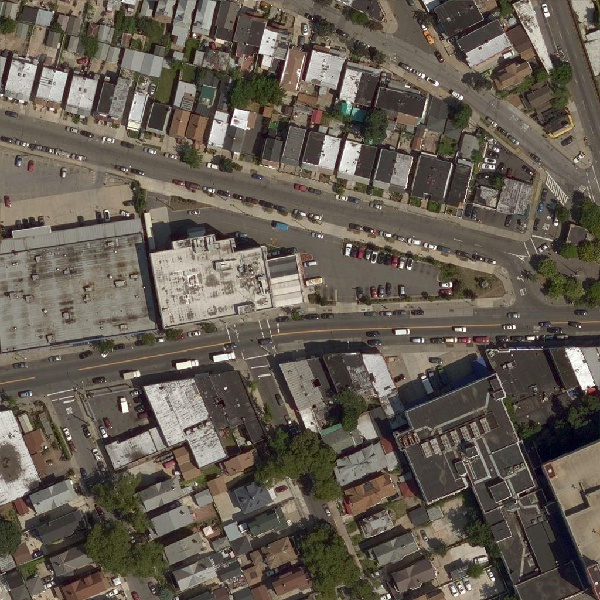
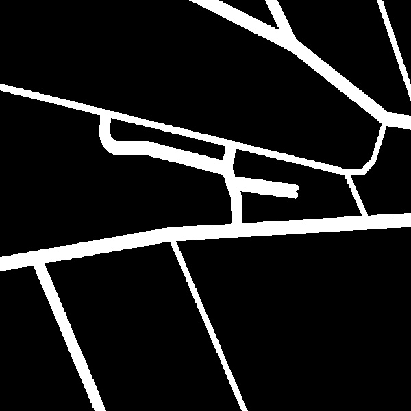
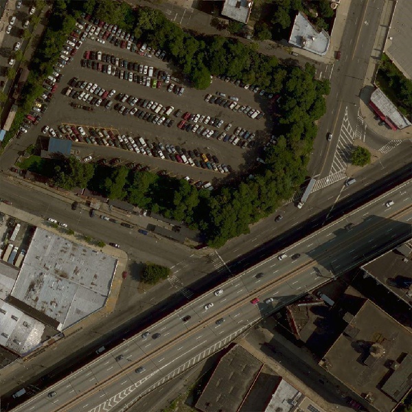
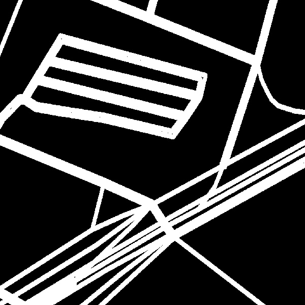
Figure 4: Our dataset: (left) example image, (middle) road mask, and (right) speed mask (rendered using a random time). Notice that speed data is not available for every road at every time.

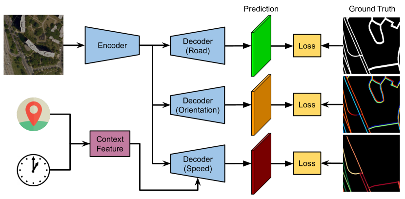
Figure 5: An overview of our network architecture.

4 Modeling Traffic Flow

We propose a novel CNN that fuses high-resolution overhead imagery, location, and time to estimate a dynamic model of traffic flow. We can think of our task as learning a conditional probability distribution over velocity, $P(\vec{v}|S(l),l,t)$, where $l$ is a latitude-longitude coordinate, $S(l)$ is an overhead image centered at that location, and $t$ represents the time.

4.1 Architecture Overview

We propose a multi-task architecture that simultaneously solves three pixel-wise labeling tasks: segmenting roads, estimating orientation, and predicting traffic speeds. Our network (Figure 5) has three inputs: a location, $l$, the time, $t$, and an overhead image, $S(l)$, centered at $l$ (of size $H\times W\times C$). We build on a modern, lightweight, semantic segmentation architecture, LinkNet [7], that follows an encoder/decoder approach with skip connections between every layer. Specifically, we use LinkNet-34, which is LinkNet with a ResNet-34 [10] encoder. For our purposes, we modify the baseline architecture to a multi-task version, with a shared encoder and separate decoder for each task. Though we use LinkNet, our approach would work with any modern encoder/decoder segmentation architecture.

Integrating Location and Time Context

To make location and time-dependent traffic flow predictions, we integrate location and time into the final speed classification layers. We represent location as normalized latitude/longitude coordinates ($\mu=0,\sigma^{2}=1$). Time is parameterized as day of week (0-6) and hour of day (0-23). Each time dimension is represented as an embedding lookup with an embedding dimension of 3. To form a context feature, we concatenate the parameterized location and time embedding outputs together. The context feature is then tiled and fused in the decoder at each of the final two convolutional layers (concatenated on as additional feature channels).

Loss Function

We simultaneously optimize the entire network, in an end-to-end manner, for all three tasks. The final loss function becomes:

$$\mathcal{L}=\mathcal{L}_{road}+\mathcal{L}_{orientation}+\mathcal{L}_{speed}+\alpha_{r}\mathcal{L}_{reg},$$ (1)

where $\mathcal{L}_{road}$, $\mathcal{L}_{orientation}$, and $\mathcal{L}_{speed}$ correspond to the task-specific objective function for road segmentation, orientation estimation, and traffic speed prediction, respectively. Additionally, $\mathcal{L}_{reg}$ is a regularization term that is weighted by a scalar $\alpha_{r}$. In the following sections we detail the specifics of each task, including the architecture and respective loss terms.

4.2 Identifying Presence of Roads

The objective of the first decoder is to segment roads in an overhead image. We represent this as a binary classification task (road vs. not road) resulting in a single output per pixel ($H\times W\times 1$). The output is passed through a sigmoid activation function. We follow recent trends in state-of-the-art road segmentation [42] and formulate the objective function as a combination of multiple individual elements. The objective is:

$$\mathcal{L}_{road}=\mathcal{L}_{bce}+(1-\mathcal{L}_{dice}),$$ (2)

where $\mathcal{L}_{bce}$ is binary cross entropy, a standard loss function used in binary classification tasks, and $\mathcal{L}_{dice}$ is the dice coefficient, which measures spatial overlap.

4.3 Estimating Direction of Travel

The objective of the second decoder is to estimate the direction of travel along the road at each pixel. We represent this as a multi-class classification task over $K$ angular bins, resulting in $K$ outputs per pixel ($H\times W\times K$). A softmax activation function is applied to the output. For this task, the per-pixel loss function is categorical cross entropy:

$$\mathcal{L}_{orientation}=-\log(G(S(l);\Theta)(y)),$$ (3)

where $G(S(l);\Theta)$ represents our CNN as a function that outputs a probability distribution over the $K$ angular bins and $y$ indicates the true label. We compute road orientation, $\theta$, as the angle the road direction vector makes with the positive X axis. The valid range of values is between $-\pi$ and $\pi$ and we generate angular bins by dividing this space uniformly.

4.4 Predicting Traffic Speeds

The objective of the final decoder is to estimate local traffic speeds, taking into account the imagery, the location, and the time. Instead of predicting a single speed value for each pixel, we make angle-dependent predictions. The road speed decoder has $K$ outputs per pixel ($H\times W\times K$) and a softplus output activation, $\log(1+\exp(x))$, to ensure positivity. For a given road angle $\theta$, we compute the estimated speed as an orientation-weighted average using $w_{\mu}=e^{k\cos(\theta-\mu)}$ as the weight for each bin where $\mu$ is the angle of the corresponding bin and $k=25$ is a fixed smoothing factor. Weights are normalized to sum to one. Note that we can predict angle-dependent speeds using either the true angle if known, or the predicted angle.

For traffic speed estimation, we minimize the Charbonnier loss (also known as the Pseudo-Huber loss):

$$\mathcal{L}_{speed}=\delta^{2}(\sqrt{1+(a/\delta)^{2}}-1),$$ (4)

where $y$ and $\hat{y}$ are the observed and predicted values, respectively, and $a=y-\hat{y}$ is their residual. The Charbonnier loss is a smooth approximation of the Huber loss, where $\delta$ controls the steepness. In addition, we add a regularization term, $\mathcal{L}_{reg}$, to reduce noise and encourage spatial smoothness. For this we use the anisotropic version of total variation, $f(x)=(x_{i+1,j}-x_{i,j})^{2}+(x_{i,j+1}-x_{i,j})^{2}$, averaged over all pixels, $i,j$, in the raw output.

Region Aggregation

The target labels for traffic speed are provided as averages over road segments, which means we cannot use a traditional per-pixel loss. The naïve approach would be to assume the speed is constant across the entire road segment, which would lead to over-smoothing and incorrect predictions. Instead, we use a variant of the region aggregation layer [12], adapted to compute the average of the per-pixel estimated speeds over the segment. We optimize our network to generate per-pixel speeds such that the segment averages match the true speed. In practice we predict angle-dependent speeds, compute the orientation-weighted average, and then apply region aggregation; finally, computing the average loss over road segments.

4.5 Implementation Details

Our methods are implemented using PyTorch [22] and optimized using RAdam [16] ($\lambda=10^{-3}$) with Lookahead [39] ($k=5,\alpha=0.5$). We initialize the encoder with weights from a network pretrained on ImageNet. For fairness, we train all networks with a batch size of 6 for 50 epochs, on random crops of size $640\times 640$. We use $K=16$ angular bins and set $\alpha_{r}=10^{-2}$, chosen empirically. For this work, we set $\delta=2$. Our networks are trained in a dynamic manner; instead of rendering a segmentation mask at every possible time, for every training image, we sample a time during training and dynamically render the speed mask. The alternative would be to pregenerate over a million segmentation masks. Additionally, we train the orientation and speed estimation decoders in a sparse manner by sampling pixels along road segments (every one meter along the segment and up to two meters on each side, perpendicularly) and computing orientation from corresponding direction vectors. For road segmentation, we buffer the road geometries (two meter half width) and do not sample. Model selection is performed using the validation set.

5 Evaluation

We train and evaluate our method using the dataset described in Section 3. We primarily evaluate our model for traffic speed estimation, but present quantitative and qualitative results for both road segmentation and orientation estimation.

5.1 Ablation Study

We conducted an extensive ablation study to evaluate the impact of various components of our proposed architecture. For evaluation, we use the reserved test set, but evaluate on a single timestep per image (randomly selected from the observed traffic speeds using a fixed seed). When computing metrics, we represent speeds using kilometers per hour and average predictions along each road segment before comparing to the ground truth.

5.1.1 Impact of Multi-Task Learning

For our first experiment, we quantify the impact of multi-task learning for estimating traffic speeds. In other words, we evaluate whether or not simultaneously performing the road segmentation and orientation estimation tasks improves the results for estimating traffic speeds. We compare our full method (Section 4) to variants with subsets of the multi-task components. The results of this experiment are shown in Table 1 for three metrics: root-mean-square error (RMSE), mean absolute error (MAE) and the coefficient of determination ($R^{2}$).

As observed, the multi-task nature of our architecture improves the final speed predictions. Adding the road segmentation and orientation estimation tasks improves results over a baseline that only estimates traffic speed, with the best performing model integrating both tasks. Our results are in line with previous work [40] that demonstrates multi-task learning can be helpful when the auxiliary tasks are related to the primary task. For the remainder of the ablation study, we only consider our full architecture that performs all three tasks.

Table 1: Evaluating the impact of multi-task learning for traffic speed estimation.

Road	Orientation	RMSE	MAE	$R^{2}$
✗	✗	10.87	8.35	0.442
✗	✓	10.78	8.21	0.452
✓	✗	10.73	8.19	0.456
✓	✓	10.66	8.10	0.464

5.1.2 Impact of Region Aggregation

Next, we consider how region aggregation affects traffic speed estimation. As described in Section 4, the target speeds for the traffic speed estimation task are averages over each road segment. Here we compare two approaches for training using these labels: 1) naïvely replicating the target labels spatially across the entire road segment, and 2) our approach that integrates a variant of the region aggregation layer [12], which enables prediction of per-pixel speeds such that the segment averages match the ground-truth speed label for that segment.

To evaluate both approaches, we average predictions along each road segment and compare to the true traffic speed label. The baseline method achieves an RMSE score of $11.10$, which is worse than our method (RMSE = $10.66$). Additionally, we show some qualitative results of the two approaches in Figure 6. Our method which incorporates region aggregation (top) is better able to capture real-world properties of traffic speed, such as slowing down at intersections or around corners. For the remainder of the ablation study, we only consider methods which were optimized and evaluated using region aggregation.

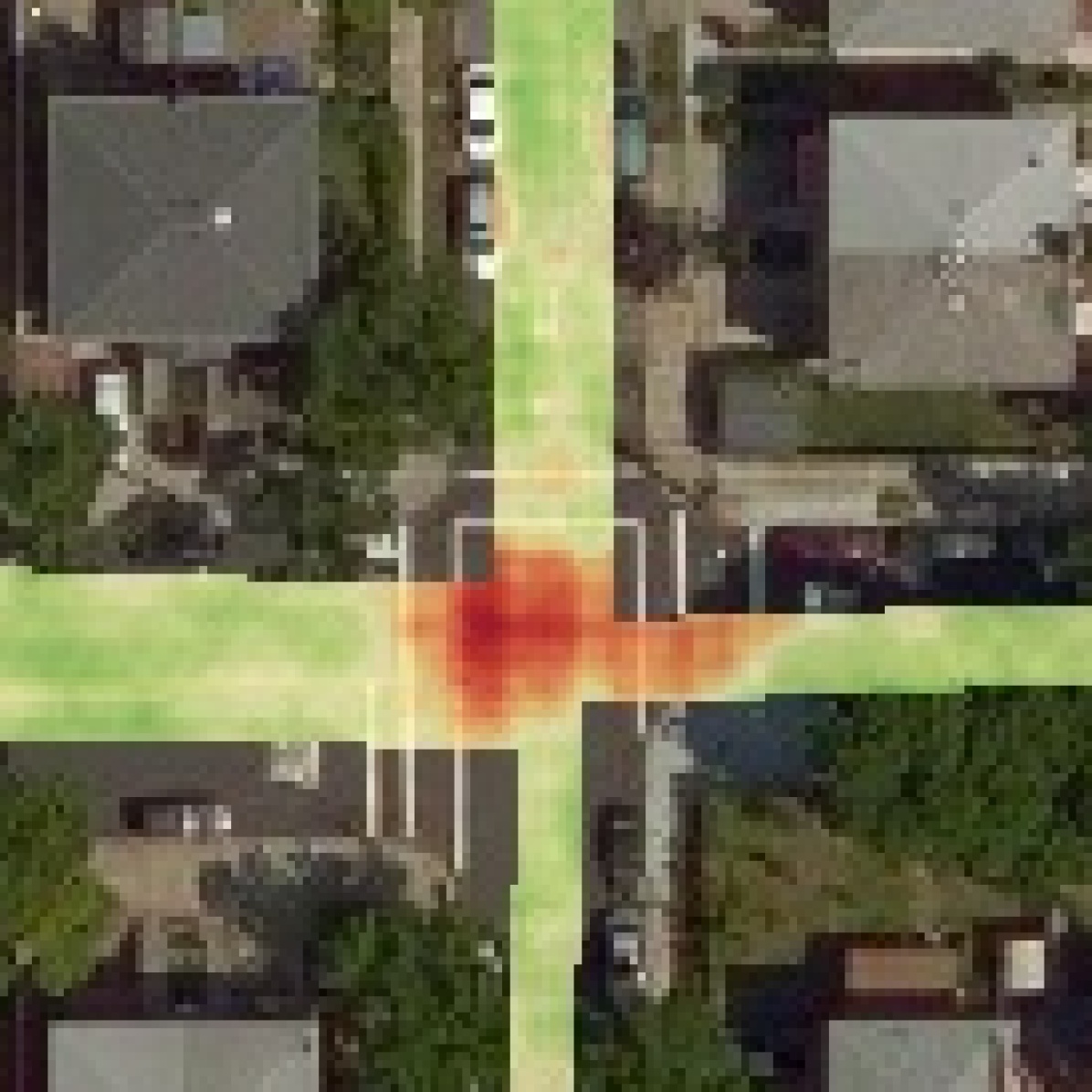
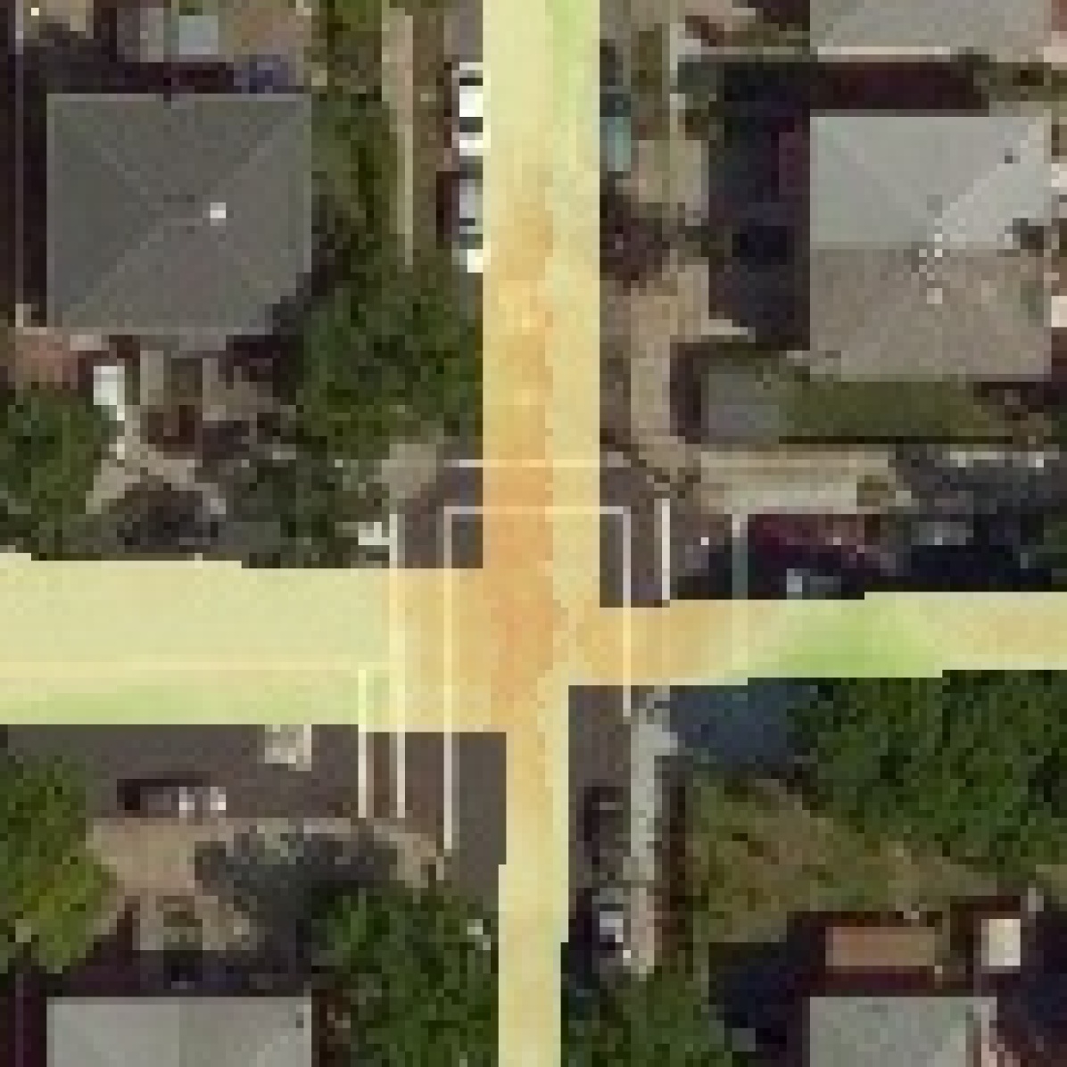
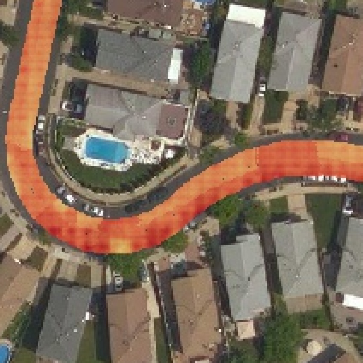
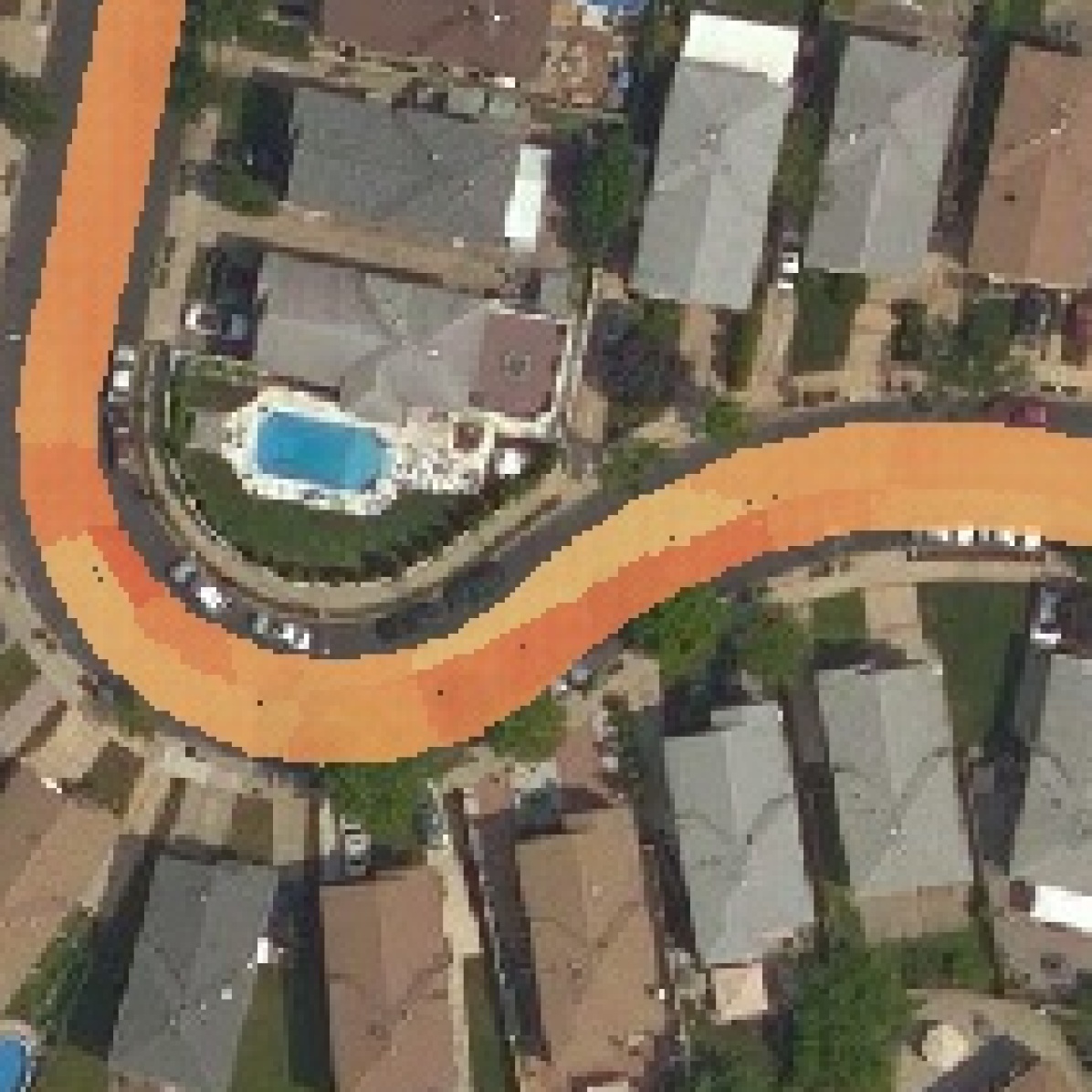
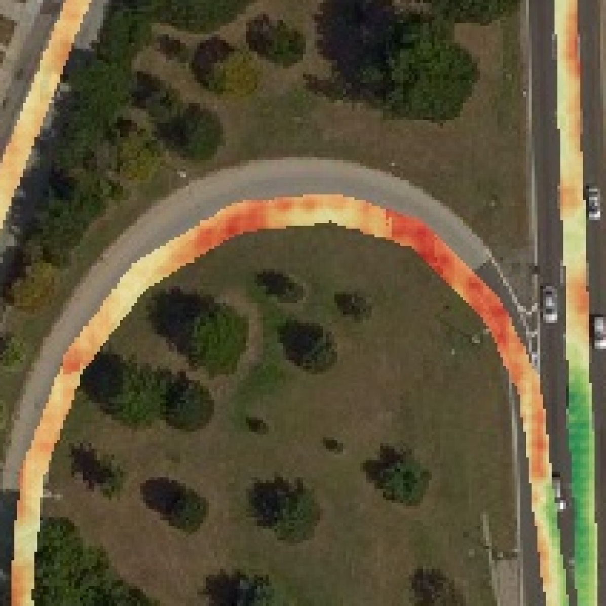
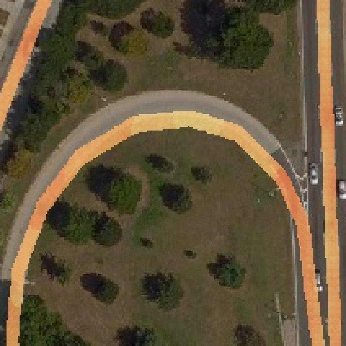
Figure 6: Qualitative examples showing the impact of region aggregation (top) versus no aggregation (bottom).

5.1.3 Impact of Location and Time Context

Finally, we evaluate how integrating location and time context impacts our traffic speed predictions. For this experiment, we compare against several baseline methods that share many low-level components with our proposed architecture. Our full model includes all three components image, loc, and time. For the metadata only approaches, those without image, we use our proposed architecture, but omit all layers prior to concatenating in the context feature.

The results of this experiment are shown in Table 2. Both location and time improve the resulting traffic speed predictions. Our method, which integrates overhead imagery, location, and time, outperforms all other models. Additionally, we show results for road segmentation (F1 score) and orientation estimation (top-1 accuracy). These tasks do not rely on location and time, so their performance is comparable, but our method still performs best.

Table 2: Evaluating the impact of location and time context.

	Road	Orientation	Speed
	(F1 Score)	(Accuracy)	(RMSE)
loc	–	–	13.38
time	–	–	14.06
loc, time	–	–	13.14
image	0.796	75.05%	11.35
image, loc	0.798	75.63%	10.95
image, time	0.798	76.04%	10.68
image, loc, time	0.800	76.32%	10.66

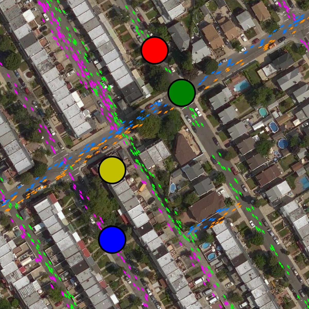
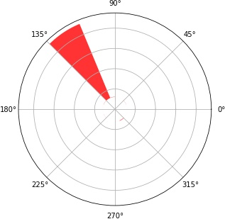
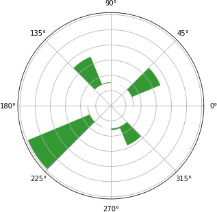
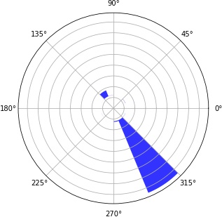
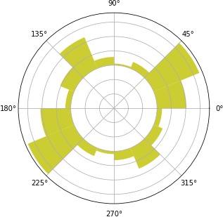
Figure 7: Estimating directions of travel. (left) An overhead image and estimated orientation represented as a flow field. (right) Predicted distributions over orientation for corresponding dots in the image. (top, right) The predicted distribution for the green dot correctly identifies multiple possible directions of travel. This makes sense as the location in the image is at an intersection.

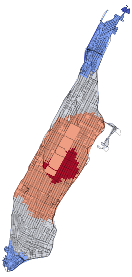
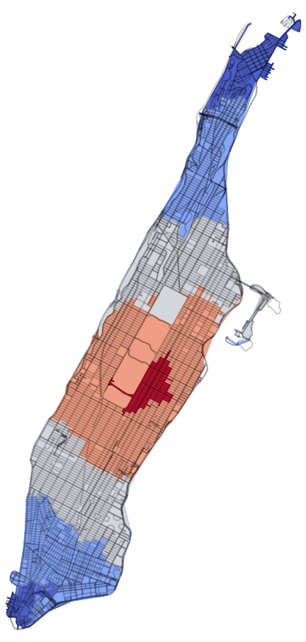
(a) Manhattan

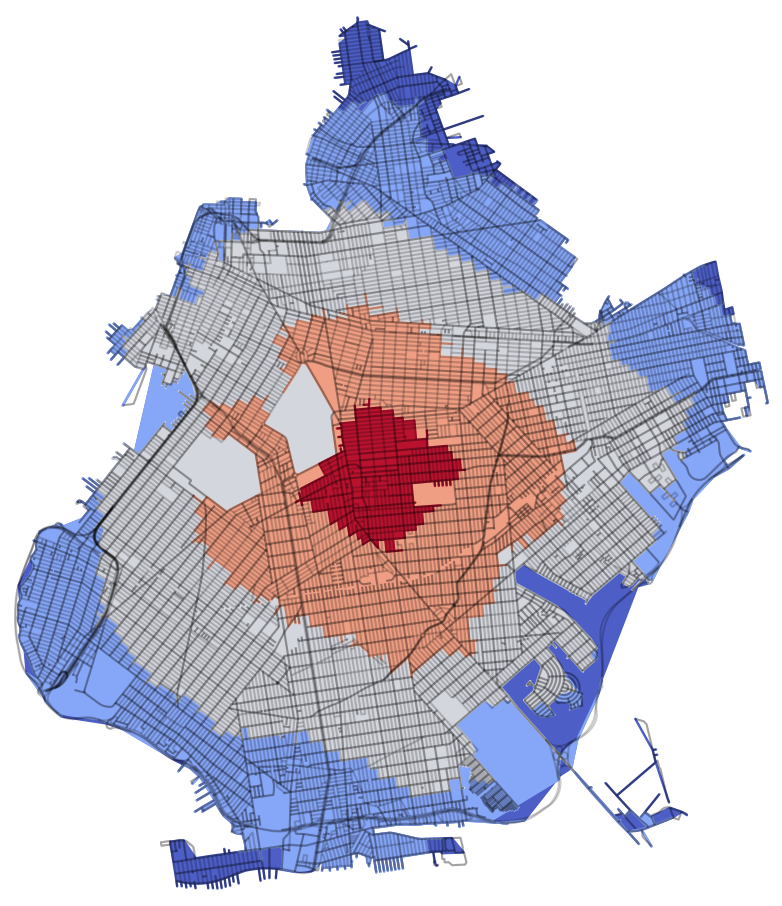
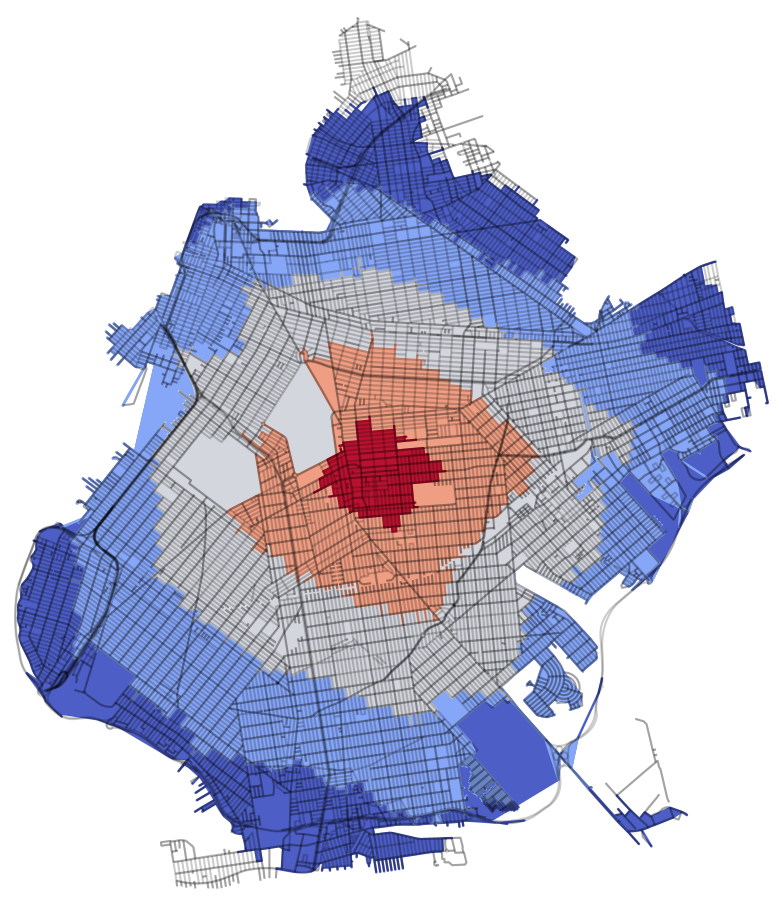
(b) Brooklyn

Figure 8: Isochrone maps obtained by using our approach. Isocontours represent the amount of time that it would take to travel to all locations within the borough, starting from the center. For each borough the maps correspond to (left) Monday at 4am and (right) Monday at 8am. As anticipated, travel is more restrictive at 8am, likely corresponding to rush hour traffic.

5.2 Visualizing Traffic Flow

In this section, we qualitatively evaluate our proposed methods ability to capture spatial and temporal patterns in traffic flow. First, we examine how well our approach is able to estimate directions of travel. Figure 7 (left) visualizes the predicted per-pixel orientation for an overhead image, overlaid as a vector field (colored by predicted angle). As observed, our method is able to capture primary directions of travel, including differences in one way and bidirectional roads. Additionally, Figure 7 (right) shows radial histograms representing the predicted distributions over orientation for corresponding color-coded dots in the overhead image. For example, the predicted distribution for the green dot (top, right), which represents an intersection in the image, correctly identifies several possible directions of travel. Alternatively, the predicted distribution for the yellow dot is more uniform, which makes sense as the location is not a road.

Next, we examine how our model captures temporal trends in traffic flow. Figure 9 visualizes traffic speed predictions for a residential road segment colored in red. Figure 9 (right) shows the predicted speeds for this segment versus the day of the week, with each day representing twenty four hours. As observed, the predicted speeds capture temporal trends both daily, and over the course of the full week. Finally, Figure 1 shows predicted traffic speeds for The Bronx, New York City for Monday at 4am (left) versus Monday at 8am (right). As expected, there is a large slow down likely corresponding to rush hour. These results demonstrate that our model is capturing meaningful patterns in both space and time.

5.3 Application: Generating Travel Time Maps

Our approach can be used to generate dynamic traffic maps at the scale of a city. To demonstrate this, we generate travel time maps at different times. We use OSMnx [6], a library for modeling street networks from OpenStreetMap, to represent the underlying street network topology for New York City as a graph. Our approach is as follows. For each image in our dataset, we estimate traffic speeds at a given time. Then we update the edge weights of the graph (corresponding to each road segment) to represent travel times using the length of each segment in meters and our traffic speed predictions. For any road segment not represented in our dataset, we use the average predicted traffic speed for that time. Figure 8 shows several results, visualized as isochrone maps that depict areas of equal travel time.

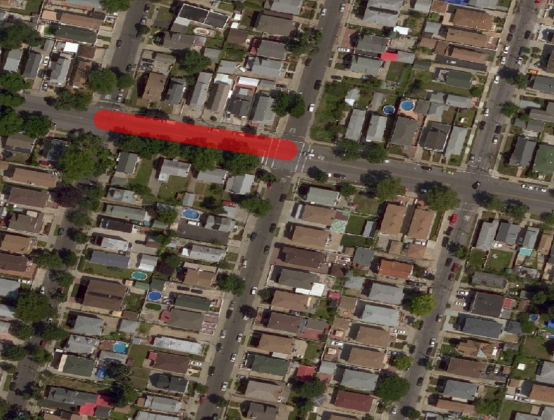
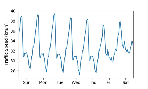
Figure 9: Visualizing how predicted speeds for a segment capture daily and weekly trends.

6 Conclusion

Understanding traffic flow is important and has many potential implications. We developed a method for dynamically modeling traffic flow using overhead imagery. Though our method incorporates time, a unique overhead image is not required for every timestamp. Our model is conditioned on location and time metadata and can be used to render dynamic city-scale traffic maps. To support our efforts, we introduced a novel dataset for fine-grained road understanding. Our hope is that this dataset will inspire further work in the area of image-driven traffic modeling. By simultaneously optimizing for road segmentation, orientation estimation, and traffic speed prediction, our method can be applied for understanding traffic flow patterns in novel areas. Potential applications of our method include assisting urban planners, augmenting routing engines, and for providing a general understanding of how to traverse an environment.

Acknowledgements We gratefully acknowledge the financial support of NSF CAREER grant IIS-1553116.

Supplemental Material :
Dynamic Traffic Modeling from Overhead Imagery

This document contains additional details and experiments related to our methods.

1 Dynamic Traffic Speeds Dataset

We presented a new dataset for fine-grained road understanding containing $11\,902$ non-overlapping overhead images, associated road attributes, and historical traffic data. Figure S1 shows the spatial coverage of our dataset, with yellow, blue, and magenta corresponding to the location of training, testing, and validation images, respectively. Figure S3 shows example images from the dataset along with the road mask and a speed mask rendered using a random time (road segments buffered to two meter half width).

We also report some statistics of the underlying historical traffic speed data. Note that these numbers are computed on the provided aggregated traffic speed data, which is then further aggregated by day of week and hour of day. The average road segment speed in NYC for 2018 (averaging road segments over time first, then averaging across segments) is approximately $30.47$ km/h ($\sigma=11.99$). In Figure S2, we visualize the average road segment speed versus time. Additionally, Figure S4 shows the average speed according to OpenStreetMap’s road type classification.

2 Extended Evaluation

In the main document, we presented an evaluation for traffic speed estimation where each image in the test set was associated with a random time to represent the ground truth speed data. These image/time pairs were then fixed for all methods evaluated. Here we explore a macro evaluation, where we consider the relationship between performance and time. Table S1 shows the results of this experiment for a subset of times. When computing metrics, we select all images in the test set which have at least one segment with empirical traffic speed data at the time of interest. Then, we compute metrics for each time and average the result (treating all times equally). For this experiment, we consider Monday and Saturday and selected the following hours of the day: 12am, 4am, 8am, 12pm, 5pm, and 8pm. Consistent with our earlier results, our method that integrates location and time outperforms an image-only baseline.

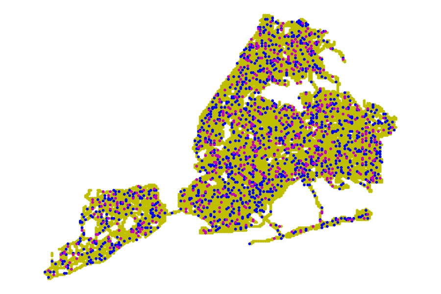
Figure S1: Coverage of our dataset. Each dot corresponds to a non-overlapping overhead image (yellow training, blue testing, magenta validation).

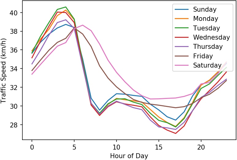
Figure S2: Average road segment speed versus time.

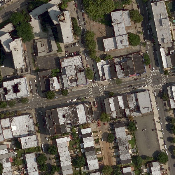
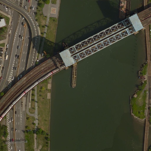
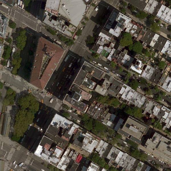
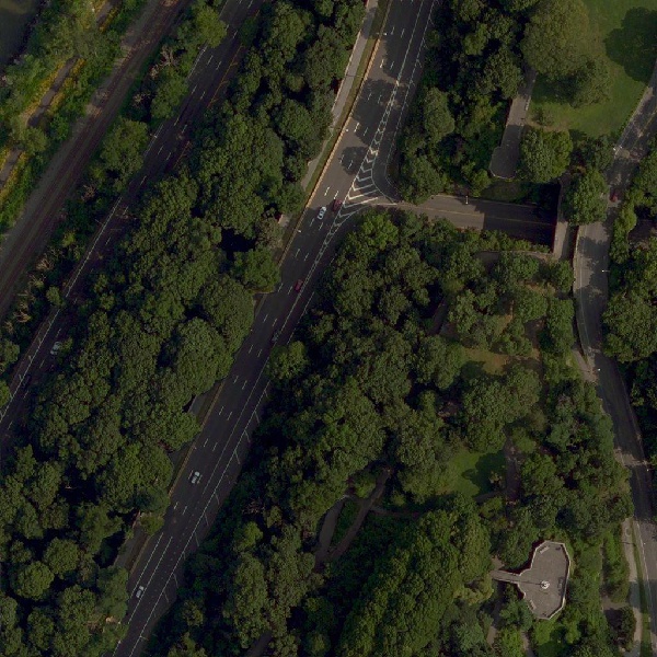
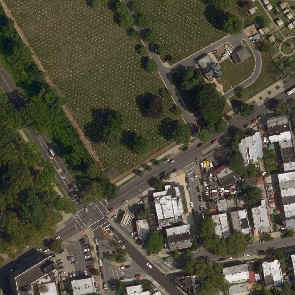
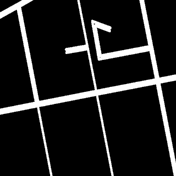
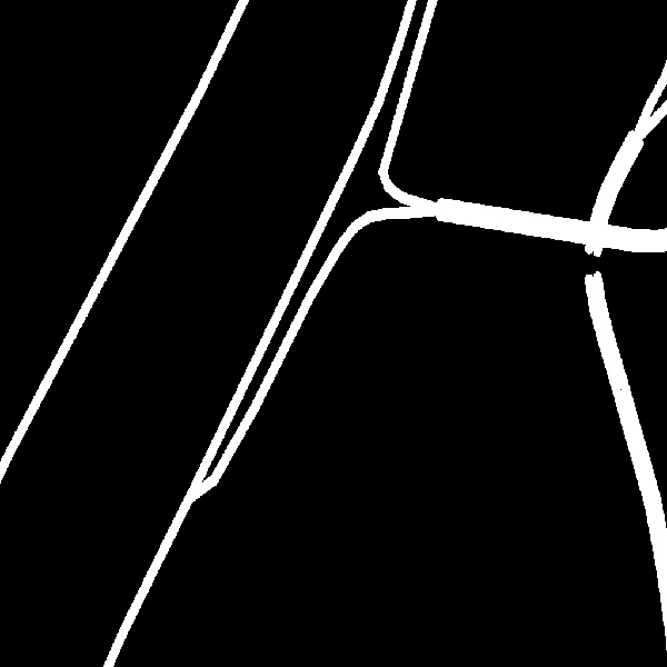
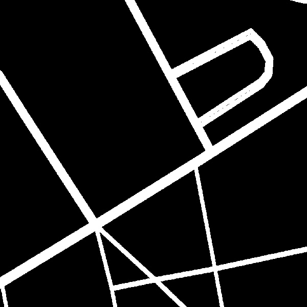
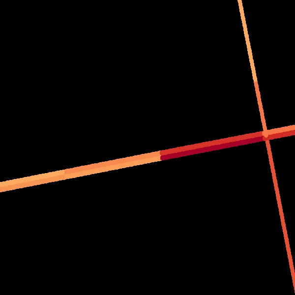
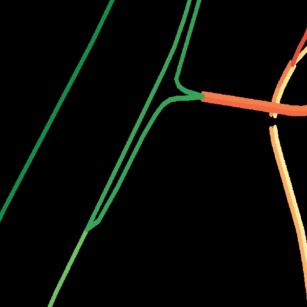
Figure S3: Examples from our dataset: (top) image, (middle) road mask, and (bottom) speed mask rendered using a random time (where red is slower and green faster). Notice that historical speed data is not available for every road at every time.

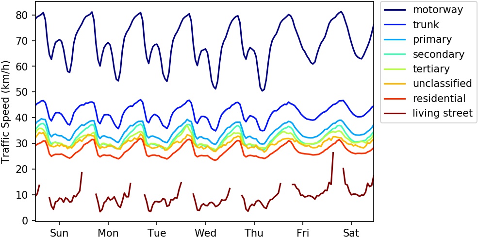
Figure S4: Average road segment speed versus time, where each road is categorized by its OpenStreetMap road type classification.

Table S1: Quantitative evaluation of traffic speed estimation (RMSE).

	image	Ours (uniform)	Ours
Monday (4am)	15.82	13.31	13.24
Monday (12pm)	10.96	10.59	10.41
Saturday (5pm)	10.65	10.39	10.36
Saturday (8pm)	10.43	10.32	10.27
Overall	11.903	11.145	11.134

2.1 Impact of Angle-Dependent Speeds

In our approach, we estimate angle-dependent speeds as opposed to predicting a single speed per location. The intuition behind this idea is that speed tends to depend on direction, e.g., a bridge that crosses over a highway. Following the above evaluation scheme, we compare our strategy of making angle-dependent speed predictions to a baseline that instead uses uniform weights. In other words, we replace the orientation-weighted average with an equal-weighted average. The results are shown in Table S1. Our full approach outperforms the uniform variant.

Shortest Distance	Travel Time (Monday at 4am)	Travel Time (Monday at 8am)

Figure S5: Using dynamic traffic speed predictions to augment route generation. The routes correspond to (left) the shortest path in terms of total length, (middle) travel time on a Monday at 4am, and (right) travel time on a Monday at 8am. Note that for the travel time routes, edge weights are represented by traversal times and computed using the length of the road segment and corresponding traffic speed estimated by our approach.

3 Application: Augmenting Routing Engines

Our method can be applied to generate optimal travel routes that take into account traffic speeds at different times. For this experiment, we use the OSMnx library [6] to represent the underlying road topology. We compute the traversal time of each edge based on the road segment length and our speed estimate. Figure S5 shows the results of this experiment for a route in Queens, New York. Figure S5 (left) shows the route corresponding to shortest overall distance. Figure S5 (middle) shows the route corresponding to the shortest travel time on Monday at 4am. Figure S5 (right) shows the route corresponding to the shortest travel time on Monday at 8am.

4 Additional Results

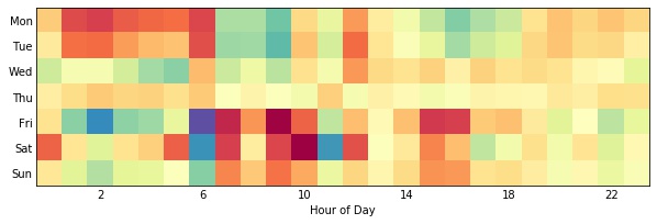
Figure S6: Visualizing the learned time embedding.

Visualizing the Time Embedding

In Figure S6 we visualize the learned time embedding. To form this image, we take the three dimensional embedding for each dimension of time (day of shape $7\times 3$ and hour of shape $24\times 3$) and form a false color image of shape $7\times 24\times 3$ by broadcasting; then average across channels. As observed, the learned embeddings are clearly capturing traffic speed patterns related to time. For example, on Friday and Saturday the embedding reflects much larger values (red) around the middle of the day as opposed to other days of the week. This makes sense as many people work half days on Friday and leave work early or take the family shopping on Saturday. This result also agrees with the temporal patterns for traffic speed shown in Figure S2.

Qualitative Results

Figure S7 shows several example images alongside the ground-truth road mask and the prediction from our approach. Similarly, Figure S8 shows additional examples for orientation estimation, visualized as a flow field for a subset of points.

Image	Target	Prediction	Error

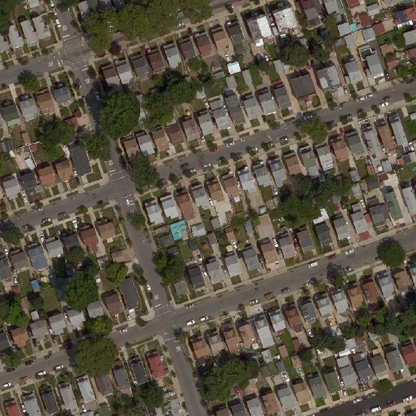
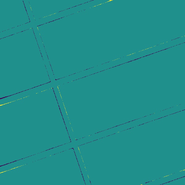
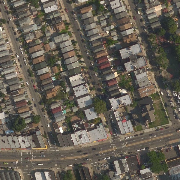
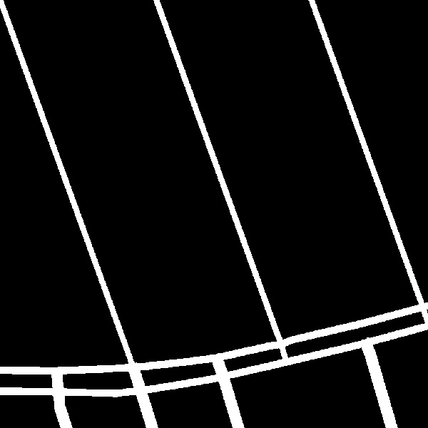
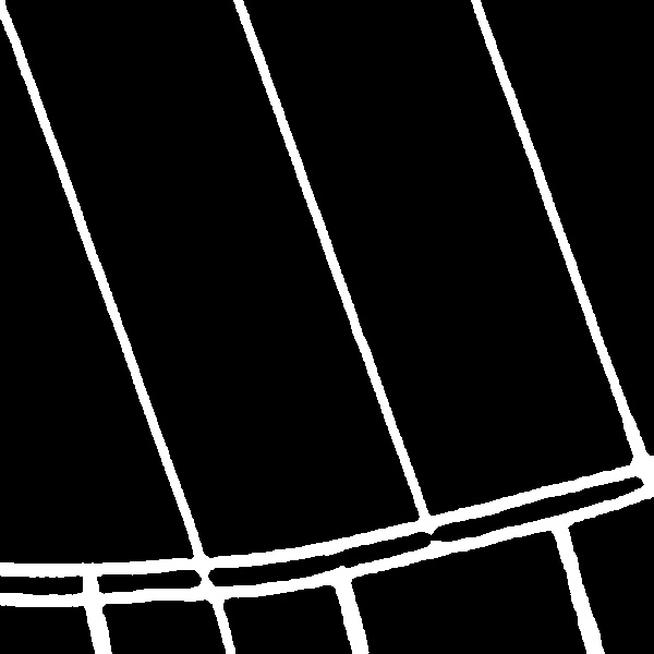
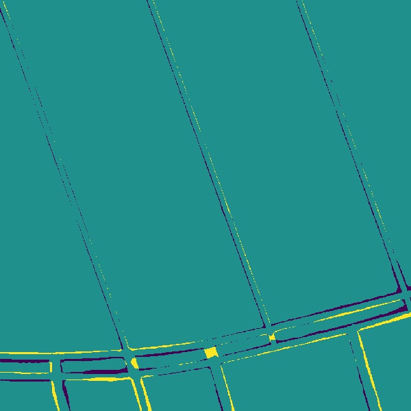
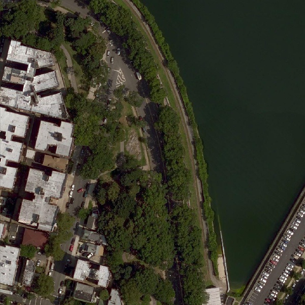
Figure S7: Qualitative results from road segmentation. The error image (right) shows false positives (negatives) color coded as purple (yellow).

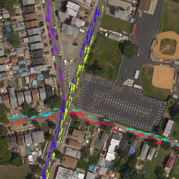
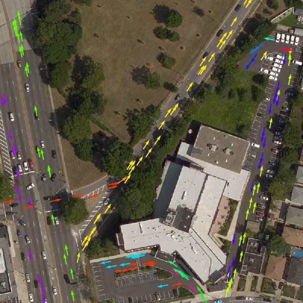
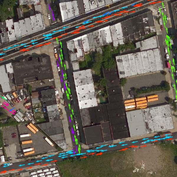
Figure S8: Using our approach to estimate directions of travel (visualized as flow fields).

References

- [1] Data retrieved from Uber Movement, (c) 2020 Uber Technologies, Inc. https://movement.uber.com.
- [2] Uber Movement: Speeds calculation methodology. Technical report, Uber Technologies, Inc., 2019.
- [3] Afshin Abadi, Tooraj Rajabioun, and Petros A Ioannou. Traffic flow prediction for road transportation networks with limited traffic data. IEEE Transactions on Intelligent Transportation Systems, 16(2):653–662, 2014.
- [4] Adrian Albert, Jasleen Kaur, and Marta C Gonzalez. Using convolutional networks and satellite imagery to identify patterns in urban environments at a large scale. In ACM SIGKDD International Conference on Knowledge Discovery and Data Mining, 2017.
- [5] Anil Batra, Suriya Singh, Guan Pang, Saikat Basu, CV Jawahar, and Manohar Paluri. Improved road connectivity by joint learning of orientation and segmentation. In IEEE Conference on Computer Vision and Pattern Recognition, 2019.
- [6] Geoff Boeing. OSMnx: New methods for acquiring, constructing, analyzing, and visualizing complex street networks. Computers, Environment and Urban Systems, 65:126–139, 2017.
- [7] Abhishek Chaurasia and Eugenio Culurciello. LinkNet: Exploiting encoder representations for efficient semantic segmentation. In IEEE Visual Communications and Image Processing, 2017.
- [8] Abhimanyu Dubey, Nikhil Naik, Devi Parikh, Ramesh Raskar, and César A Hidalgo. Deep learning the city: Quantifying urban perception at a global scale. In European Conference on Computer Vision, 2016.
- [9] Adam Van Etten. City-scale road extraction from satellite imagery v2: Road speeds and travel times. In IEEE Winter Conference on Applications of Computer Vision, 2020.
- [10] Kaiming He, Xiangyu Zhang, Shaoqing Ren, and Jian Sun. Deep residual learning for image recognition. In IEEE Conference on Computer Vision and Pattern Recognition, 2016.
- [11] Shuai Hua, Manika Kapoor, and David C Anastasiu. Vehicle tracking and speed estimation from traffic videos. In CVPR Workshop on AI City Challenge, 2018.
- [12] Nathan Jacobs, Adam Kraft, Muhammad Usman Rafique, and Ranti Dev Sharma. A weakly supervised approach for estimating spatial density functions from high-resolution satellite imagery. In ACM SIGSPATIAL International Conference on Advances in Geographic Information Systems, 2018.
- [13] Daniel Krajzewicz, Jakob Erdmann, Michael Behrisch, and Laura Bieker. Recent development and applications of sumo-simulation of urban mobility. International Journal On Advances in Systems and Measurements, 5(3&4), 2012.
- [14] Stefan Krauß. Microscopic modeling of traffic flow: Investigation of collision free vehicle dynamics. PhD thesis, University of Cologne, 1998.
- [15] John M Levy. Contemporary urban planning. Taylor & Francis, 2016.
- [16] Liyuan Liu, Haoming Jiang, Pengcheng He, Weizhu Chen, Xiaodong Liu, Jianfeng Gao, and Jiawei Han. On the variance of the adaptive learning rate and beyond. In International Conference on Learning Representations, 2020.
- [17] Gellért Máttyus, Wenjie Luo, and Raquel Urtasun. DeepRoadMapper: Extracting road topology from aerial images. In IEEE International Conference on Computer Vision, 2017.
- [18] Gellért Máttyus, Shenlong Wang, Sanja Fidler, and Raquel Urtasun. HD Maps: Fine-grained road segmentation by parsing ground and aerial images. In IEEE Conference on Computer Vision and Pattern Recognition, 2016.
- [19] Michael D Meyer and Eric J Miller. Urban transportation planning: a decision-oriented approach. McGraw-Hill, 1984.
- [20] Volodymyr Mnih and Geoffrey E Hinton. Learning to detect roads in high-resolution aerial images. In European Conference on Computer Vision, 2010.
- [21] Illah Nourbakhsh, Randy Sargent, Anne Wright, Kathryn Cramer, Brian McClendon, and Michael Jones. Mapping disaster zones. Nature, 439(7078):787, 2006.
- [22] Adam Paszke, Sam Gross, Francisco Massa, Adam Lerer, James Bradbury, Gregory Chanan, Trevor Killeen, Zeming Lin, Natalia Gimelshein, Luca Antiga, et al. PyTorch: An imperative style, high-performance deep learning library. In Advances in Neural Information Processing Systems, 2019.
- [23] Caleb Robinson, Le Hou, Kolya Malkin, Rachel Soobitsky, Jacob Czawlytko, Bistra Dilkina, and Nebojsa Jojic. Large scale high-resolution land cover mapping with multi-resolution data. In IEEE Conference on Computer Vision and Pattern Recognition, 2019.
- [24] Brian E Saelens, James F Sallis, and Lawrence D Frank. Environmental correlates of walking and cycling: findings from the transportation, urban design, and planning literatures. Annals of Behavioral Medicine, 25(2):80–91, 2003.
- [25] Tawfiq Salem, Scott Workman, and Nathan Jacobs. Learning a dynamic map of visual appearance. In IEEE Conference on Computer Vision and Pattern Recognition, 2020.
- [26] David Schrank, Bill Eisele, and Tim Lomax. 2019 urban mobility report. Technical report, Texas A&M Transportation Institute, 2019.
- [27] Stephen F Smith, Gregory Barlow, Xiao-Feng Xie, and Zachary B Rubinstein. SURTRAC: Scalable urban traffic control. Transportation Research Board Annual Meeting, 2013.
- [28] Robert Soden and Leysia Palen. From crowdsourced mapping to community mapping: The post-earthquake work of OpenStreetMap Haiti. In International Conference on the Design of Cooperative Systems, 2014.
- [29] Weilian Song, Tawfiq Salem, Hunter Blanton, and Nathan Jacobs. Remote estimation of free-flow speeds. In IEEE International Geoscience and Remote Sensing Symposium, 2019.
- [30] Weilian Song, Scott Workman, Armin Hadzic, Xu Zhang, Eric Green, Mei Chen, Reginald Souleyrette, and Nathan Jacobs. FARSA: Fully automated roadway safety assessment. In IEEE Winter Conference on Applications of Computer Vision, 2018.
- [31] Michael J Sprung, Sonya Smith-Pickel, et al. Transportation statistics annual report. Technical report, Bureau of Transportation Statistics, 2018.
- [32] Tao Sun, Zonglin Di, Pengyu Che, Chun Liu, and Yin Wang. Leveraging crowdsourced GPS data for road extraction from aerial imagery. In IEEE Conference on Computer Vision and Pattern Recognition, 2019.
- [33] Tim Triplett, Rob Santos, Sandra Rosenbloom, and Brian Tefft. American driving survey: 2014–2015. Technical report, The American Automobile Association, 2016.
- [34] Dong Wang, Junbo Zhang, Wei Cao, Jian Li, and Yu Zheng. When will you arrive? Estimating travel time based on deep neural networks. In AAAI Conference on Artificial Intelligence, 2018.
- [35] Scott Workman, Richard Souvenir, and Nathan Jacobs. Wide-area image geolocalization with aerial reference imagery. In IEEE International Conference on Computer Vision, 2015.
- [36] Scott Workman, Richard Souvenir, and Nathan Jacobs. Understanding and mapping natural beauty. In IEEE International Conference on Computer Vision, 2017.
- [37] Scott Workman, Menghua Zhai, David J. Crandall, and Nathan Jacobs. A unified model for near and remote sensing. In IEEE International Conference on Computer Vision, 2017.
- [38] Junbo Zhang, Yu Zheng, and Dekang Qi. Deep spatio-temporal residual networks for citywide crowd flows prediction. In AAAI Conference on Artificial Intelligence, 2017.
- [39] Michael R Zhang, James Lucas, Geoffrey Hinton, and Jimmy Ba. Lookahead optimizer: k steps forward, 1 step back. In Advances in Neural Information Processing Systems, 2019.
- [40] Zhanpeng Zhang, Ping Luo, Chen Change Loy, and Xiaoou Tang. Facial landmark detection by deep multi-task learning. In European Conference on Computer Vision, 2014.
- [41] Bolei Zhou, Agata Lapedriza, Aditya Khosla, Aude Oliva, and Antonio Torralba. Places: A 10 million image database for scene recognition. IEEE Transactions on Pattern Analysis and Machine Intelligence, 40(6):1452–1464, 2017.
- [42] Lichen Zhou, Chuang Zhang, and Ming Wu. D-LinkNet: LinkNet with pretrained encoder and dilated convolution for high resolution satellite imagery road extraction. In CVPR Workshop on DeepGlobe, 2018.