A closed form scale bound for the $(\epsilon,\delta)$-differentially private Gaussian Mechanism valid for all privacy regimes

Abstract

The standard closed form lower bound on $\sigma$ for providing $(\epsilon,\delta)$-differential privacy by adding zero mean Gaussian noise with variance $\sigma^{2}$ is $\sigma>\Delta\sqrt{2}(\epsilon^{-1})\sqrt{\log\left(5/4\delta^{-1}\right)}$ for $\epsilon\in(0,1)$. We present a similar closed form bound $\sigma\geq\Delta(\epsilon\sqrt{2})^{-1}\left(\sqrt{az+\epsilon}+s\sqrt{az}\right)$ for $z=-\log(4\delta(1-\delta))$ and $(a,s)=(1,1)$ if $\delta\leq 1/2$ and $(a,s)=(\pi/4,-1)$ otherwise. Our bound is valid for all $\epsilon>0$ and is always lower (better). We also present a sufficient condition for $(\epsilon,\delta)$-differential privacy when adding noise distributed according to even and log-concave densities supported everywhere.

1 Introduction

Differential privacy [4] is an emerging standard for individual data privacy. In essence, differential privacy is a bound on any belief update about an individual on receiving a result of a differentially private randomized computation. Critical for the utility of such results is minimizing the random perturbation required for a given level of privacy.

Formally, let a database $d$ be a collection of record values from some set $V$. Two databases $d$ and $d^{\prime}$ are neighboring if one can be obtained from the other by adding one record. Let $\mathcal{N}$ be the set of all pairs of neighboring databases. Then following Dwork et al. [4, 5] we define differential privacy as follows.

Definition 1 ($(\epsilon,\delta)$-differential privacy [4, 5]).

A randomized algorithm $M$ is called $(\epsilon,\delta)$-differentially private if for any measurable set $S$ of possible outputs and all $(d,d^{\prime})\in\mathcal{N}$

$$\Pr(M(d)\in S)\leq e^{\epsilon}\Pr(M(d^{\prime})\in S)+\delta,$$

where the probabilities are over randomness used in $M$. By $\epsilon$-differential privacy we mean $(\epsilon,0)$-differential privacy.

A standard mechanism for achieving $(\epsilon,\delta)$-differential privacy is that of adding zero mean Gaussian noise to a statistic, called the Gaussian Mechanism. A primary reason for the popularity of the Gaussian Mechanism is that the Gaussian distribution is closed under addition. However, Gaussian noise requires $\delta>0$, which represents a relaxation of the stronger $(\epsilon,0)$-differential privacy that is not uncontroversial [8]. On the positive side, a non-zero $\delta$ allows, among others, for better composition properties than $(\epsilon,0)$-differential privacy [6]. The exploitation of the composition benefits of using Gaussian noise can be observed in an application to deep learning by Abadi et al.[1].

To achieve $(\epsilon,\delta)$-differential privacy, the variance $\sigma^{2}$ is carefully tuned taking into account the sensitivity $\Delta$ of the statistic, i.e., the maximum change in the statistic resulting from adding or removing any individual record from any database. Of prime importance is to minimize $\sigma$ while still achieving $(\epsilon,\delta)$-differential privacy as higher $\sigma$ generally decreases the utility of the now noisy statistic.

In their Theorem A.1 [3], Dwork and Roth state that $(\epsilon,\delta)$-differential privacy is achieved for $\epsilon\in(0,1)$ if

$$\sigma>s(\epsilon,\delta,\Delta)={\frac{{\Delta}\,\sqrt{2}}{{\epsilon}}\sqrt{\log\left({\frac{5}{4\,{\delta}}}\right)}}.$$ (1)

The above bound (1) is essentially the standard closed form used for the Gaussian Mechanism, and we will refer to it as such in the following. Notably, the restriction $\epsilon\in(0,1)$ can present non-obvious pitfalls in addition to the explicit restriction to privacy regimes with $\epsilon<1$. For example consider the representation of $\epsilon$ as a function derived from the standard bound (1) (ignoring strict inequalities)

$$\epsilon(\delta,\sigma,\Delta) ={\frac{{\Delta}\,\sqrt{2}}{{\sigma}}\sqrt{\log\left({\frac{5}{4\,{\delta}}}\right)}}.$$ (2)

A use of the above function can, for example, be found in [11], Section 4. As the magnitude of $\delta$ is associated with the failure of guaranteeing strong $\epsilon$-differential privacy, it is sometimes stated that $\delta$ should be cryptographically small. Now, the function in (2) increases as $\delta>0$ decreases, and for fixed $\sigma$ and $\Delta$, even a relatively large $\delta$ could result in $\epsilon(\delta,\sigma,\Delta)\geq 1$, which might not be obvious. For example, $\epsilon(10^{-1},1,1)>2.24$.

1.1 Main contributions

Our main contributions are twofold:

1. The closed form lower bound on $\sigma$ for achieving $(\epsilon,\delta)$-differential privacy given in Theorem 5. Unlike the standard bound, which is defined for $0<\epsilon<1$, our bound is valid for all $\epsilon>0$. In addition it is always better than the standard bound for $0<\epsilon<1$.

2. The sufficient condition for $(\epsilon,\delta)$-differential privacy for mechanisms that add noise distributed according to an even and log-concave density supported everywhere given in Lemma 2. The condition is also specialized to the zero mean Gaussian distribution in Corollary 1 and the Laplace distribution in Remark 2.

The sufficient condition in point 2. above is inspired by a sufficient condition for zero mean Gaussian noise described by Le Ny and Pappas [7]. We derive their condition from Lemma 2 as Corollary 1.

2 A few more preliminaries

We briefly recapitulate known results. In the following, we will let $\Phi$ and $\phi$ denote the standard Gaussian distribution function and density, respectively.

Definition 2.

The global sensitivity of a real-valued function $q$ on databases is

$$\Delta_{q}=\max_{(d,d^{\prime})\in\mathcal{N}}|q(d)-q(d^{\prime})|.$$

Lemma 1.

Let $X$ be distributed according to density $f:\mathbb{R}\to\mathbb{R}$. For arbitrary but fixed $x,y\in\mathbb{R}$ we have that $\Pr(X+(x-y)\in S)\leq e^{\epsilon}\Pr(X\in S)+\delta$ for all measurable $S$ implies $\Pr(X+x)\in S)\leq e^{\epsilon}\Pr(X+y\in S)+\delta$ for all measurable $S$.

Proof.

Follows directly from that if $S\subseteq\mathbb{R}$ is measurable, so is $r+S$ for any $r\in\mathbb{R}$, including $r=-y$. ∎

3 Our closed form bound

We are now ready to present our main contributions.

Lemma 2.

Let $X$ be a random variable distributed according to even density $f(x)=e^{-\psi(x)}$ where $\psi:\mathbb{R}\to\mathbb{R}$ is convex. Then for a real-valued function $q$ on databases with global sensitivity $\Delta$ and a database $d$, the mechanism returning a variate of $q(d)+sX$ is $(\epsilon,\delta)$-differentially private if

$$\Pr\left(X>\frac{x-\Delta}{s}\right)\leq\delta$$

where

$$x\leq\sup\left\{z\mid\psi\left(\frac{z}{s}\right)-\psi\left(\frac{z-\Delta}{s}\right)\leq\epsilon\right\}.$$

Proof.

First, since $\psi:\mathbb{R}\to\mathbb{R}$ is convex, $f$ is log-concave and supported everywhere. Let $f_{sX+x}$ denote the density of $sX+x$ for $x,s\in\mathbb{R},s>0$, and recall that $f_{sX+x}(w)=s^{-1}f((w-x)/s)$.

Let $d=x-y$. Due to Lemma 1 it is sufficient to show $\Pr(X+d\in S)\leq e^{\epsilon}\Pr(X\in S)+\delta$ in order to prove $\Pr(X+x\in S)\leq e^{\epsilon}\Pr(X+y\in S)+\delta$.

Since $f$ is supported everywhere, we now define for $x,y\in\mathbb{R}$ the likelihood ratio $r$ as

$$r=\frac{f_{sX+d}}{f_{sX}}.$$ (3)

Let $A=\{z\mid r(z)\leq e^{\epsilon}\}=\{z\mid\log(r(z))\leq{\epsilon}\}$ and let $A^{c}$ denote $A$’s complement. Then for measurable $S$

$$\Pr(sX+d\in S) =\Pr(sX+d\in S\cap A)+\Pr(sX+d\in S\cap A^{c}).$$

Applying (3),

$$\Pr(sX+d\in S\cap A) \leq\Pr(sX+d\in S)$$

$$=\int_{S}f_{sX}(w)r(w)dw$$

$$\leq e^{\epsilon}\int_{S}f_{sX}(w)dw=e^{\epsilon}\Pr(sX\in S).$$

Furthermore,

$$\Pr(sX+d\in S\cap A^{c})\leq\Pr(sX+d\in A^{c}).$$

This means that a sufficient condition for $(\epsilon,\delta)$-differential privacy is

$$\Pr(sX+d\in A^{c})\leq\delta.$$ (4)

Since $f$ is log-concave, $f$ is unimodal and $r$ is monotone (see, e.g., [10]). Let $d\geq 0$, since $f$ is unimodal $r$ is non-decreasing and we can write $A=\{w\leq x^{*}\mid x^{*}=\sup\{z\mid\log(r(z))\leq\epsilon\}\}$. Now, let $d\leq 0$. Then $r$ is non-increasing and we can write $A=\{w\geq x_{*}\mid x_{*}=\inf\{z\mid\log(r(z))\leq\epsilon\}\}$. If $f$ is also even, we have that $x_{*}=-x^{*}$, and, consequently, we need only check (4) for either $d\leq 0$ or $d\geq 0$. Let $d\geq 0$. Since

$$\log(r(z)) =\log\left(\frac{f((z-d)/s)}{f(z/s)}\right)$$

$$=\log(f((z-d)/s))-\log(f(z/s))$$

$$=-\psi((z-d)/s)+\psi(z/s).$$

We can write $x^{*}=\sup\{z\mid-\psi((z-d)/s)+\psi(z/s)\leq\epsilon\}$, $A=\{w\leq x^{*}\}$, and $A^{c}=\{w>x^{*}\}$. Using this, we get

$$\Pr(sX+d\in A^{c}) =\Pr(sX+d\in\{w>x^{*}\})$$

$$=\Pr(sX+d>x^{*})=\Pr(X>(x^{*}-d)/s).$$

Furthermore, $P(X>w)$ is monotone and decreasing in $w$, which means if $w\leq x^{*}$ and $d\leq\Delta$, $\Pr(X>(w-\Delta)/s)\leq\delta$ implies $\Pr(X>(x^{*}-d)/s)\leq\delta$. The proof is concluded by noting that the case for $d=y-x$ also follows from the above. ∎

Remark 1.

Lemma 2 above is restricted to even $f$. An extension without this restriction can be obtained by determining conditions for cases $d\geq 0$ and $d\leq 0$ in the proof for Lemma 2 separately. Lemma 2 would then be a corollary of this extension.

Corollary 1.

Let $Z$ be a random variable distributed according to the standard Gaussian distribution. Then for a real-valued function $q$ on databases with global sensitivity $\Delta$ and a database $d$, the mechanism returning a variate of $q(d)+\sigma Z$ is $(\epsilon,\delta)$-differentially private if

$$\Pr\left(Z>\frac{\sigma\epsilon}{\Delta}-\frac{\Delta}{2\sigma}\right)\leq\delta.$$ (5)

Proof.

The standard Gaussian density is $\phi(x)=e^{-\psi(x)}$ for $\psi(x)=\frac{\log\left(2\pi\right)}{2}+\frac{x^{2}}{2}$. It is even and $\psi$ is convex. The equation

$$\psi(x/\sigma)-\psi((x-\Delta)/\sigma)=\epsilon$$

has unique solution

$$x^{*}=\frac{\epsilon\sigma^{2}}{{\Delta}}+\frac{{\Delta}}{2}$$

for $\Delta\geq 0$. Using this solution yields

$$\frac{x^{*}-\Delta}{\sigma}=\frac{\sigma\epsilon}{\Delta}-\frac{\Delta}{2\sigma}.$$

The corollary then follows from Lemma 2. ∎

Remark 2.

For the standard Laplace distribution, $\psi(x)=\log(2)+|x|$, which is convex. Then

$$\psi\left(\frac{x}{s}\right)-\psi\left(\frac{x-\Delta}{s}\right)={\left|\frac{x}{s}\right|}-{\left|\frac{\Delta-x}{s}\right|}=\epsilon$$

reduces to $\frac{\Delta}{s}=\epsilon$ for $x\geq\Delta>0$, and $\sup\{x\mid\psi\left(\frac{x}{\Delta/\epsilon}\right)-\psi\left(\frac{x-\Delta}{\Delta/\epsilon}\right)\leq\epsilon\}=\sup\{x\mid x\geq\Delta\}=\infty$. Applying Lemma 2 we conclude that for the standard Laplace random variable $X$, the mechanism that outputs a variate of $q(d)+\Delta/\epsilon X$ is $(\epsilon,0)$-differentially private.

Lemma 3.

Let $Z$ be a random variable distributed according to the standard Gaussian distribution. Then for $\epsilon>0$, $\Delta>0$, and $\delta\in(0,1)$

$$\Pr\left(Z>\frac{\sigma\epsilon}{\Delta}-\frac{\Delta}{2\sigma}\right)\leq\delta,$$ (5)

holds if and only if $\sigma\geq b$ for

$$b={\frac{{\Delta}}{2\,{\epsilon}}\left(\Phi^{-1}\left(1-\delta\right)+\sqrt{\left(\Phi^{-1}\left(1-\delta\right)\right)^{2}+2\,{\epsilon}}\right)}$$

where $\Phi^{-1}$ is the standard Gaussian quantile function.

Proof.

Let

$$v(\sigma)=\frac{\sigma\epsilon}{\Delta}-\frac{\Delta}{2\sigma}.$$

Then, condition (5) can be written $\Pr(Z>v(\sigma))\leq\delta$. Let

$$l(\sigma) =\Pr\left(Z>v(\sigma)\right)=1-\Phi(v(\sigma))$$

$$\iff$$

$$\Phi(v(\sigma)) =1-l(\sigma)$$

$$\iff$$

$$v(\sigma) =\Phi^{-1}\left(1-l(\sigma)\right).$$ (6)

Recall that we want to find a lower bound for $\sigma$ such that $l(\sigma)\leq\delta<1$. We note that $l(\sigma)$ is decreasing in $\sigma$ if $v$ is increasing in $\sigma$. This is the case since

$$v^{\prime}(\sigma)={\frac{2\,{{\sigma}}^{2}{\epsilon}+{{\Delta}}^{2}}{2\,{\Delta}\,{{\sigma}}^{2}}}$$

is positive for all $\sigma$ and $\Delta>0$, $\epsilon>0$. Hence, we can find the sought lower bound by solving $l(b)=\delta$ for $b$. We do this by substituting $\delta$ for $l(b)$ in (6) and solving for $b>0$, yielding

$$b ={\frac{{\Delta}}{2\,{\epsilon}}\left(\Phi^{-1}\left(1-\delta\right)+\sqrt{\left(\Phi^{-1}\left(1-\delta\right)\right)^{2}+2\,{\epsilon}}\right)}.\qed$$

Remark 3.

Let $Z$ be a standard Gaussian random variable. Recall that $P(|Z|>x)\geq P(Z>x)$. This means that $P(|Z|>x)\leq\delta$ implies $P(Z>x)\leq\delta$. Applying Corollary 1 we conclude that a sufficient condition for adding Gaussian noise to achieve $(\epsilon,\delta)$-differential privacy is

$$\Pr\left(|Z|>\frac{\sigma\epsilon}{\Delta}-\frac{\Delta}{2\sigma}\right)\leq\delta.$$ (7)

Inspecting proof of the standard bound given by Dwork and Roth [3], we note that it is based on fulfilling the condition (7) above. Replacing bound (5) by the bound (7) in Lemma 3 yields that we must have

$$\sigma\geq b ={\frac{{\Delta}}{2\,{\epsilon}}\left(\Phi^{-1}\left(1-\delta/2\right)+\sqrt{\left(\Phi^{-1}\left(1-\delta/2\right)\right)^{2}+2\,{\epsilon}}\right)}>\frac{\Delta}{\sqrt{2\epsilon}}.$$

Since the above holds for all bounds fulfilling (7), this represents a generalization and sharpening of Theorem 4 in [2] that states $\sigma\geq\frac{\Delta}{\sqrt{2\epsilon}}$ for the standard bound.

Lemma 4.

Let $\Phi^{{-1}}$ be the standard Gaussian quantile function. Then for $p\in(0,1)$

$$\Phi^{-1}(p)\leq\sqrt{2}\sqrt{\log\left(\frac{1}{4p\left(1-p\right)}\right)}\cdot\begin{cases}-\frac{\sqrt{\pi}}{2},&p<\frac{1}{2},\\ 1,&p\geq\frac{1}{2}.\end{cases}$$

Proof.

It is well known that $\operatorname{erf}(x)=\operatorname{sign}(x)P(\frac{1}{2},x^{2})$, where $P$ is the regularized gamma function $P(s,x)=\frac{\gamma(s,x)}{\Gamma(s)}$ in which $\Gamma$ and $\gamma$ are the Gamma and lower incomplete Gamma functions, respectively (see, e.g., [9] 7.11.1). From [9] (8.10.11) we have that

$$(1-e^{-\alpha_{a}x})^{a}\leq P\left(a,x\right)\leq(1-e^{-\beta_{a}x})^{a}$$

for

$$\alpha_{a} =\begin{cases}1,&0<a<1,\\ d_{a},&a>1,\end{cases}$$

$$\beta_{a} =\begin{cases}d_{a},&0<a<1,\\ 1,&a>1,\end{cases}$$

$$d_{a} =(\Gamma\left(1+a\right))^{-1/a}.$$

Since $a=1/2$ in our case, get that

$$\operatorname{erf}(x)\geq\begin{cases}-\sqrt{1-{e}^{-\frac{4x^{2}}{\pi}}},&x<0,\\ \sqrt{1-e^{-x^{2}}},&x\geq 0.\end{cases}$$

and consequently

$$\operatorname{erf}^{-1}(x)\leq\begin{cases}-\frac{\sqrt{\pi}}{2}\sqrt{-\log\left(1-x^{2}\right)},&x<0,\\ \sqrt{-\log(1-x^{2})},&x\geq 0.\end{cases}$$

As $\Phi^{-1}(p)=\sqrt{2}\operatorname{erf}^{-1}(2p-1)$, the Lemma follows by substituting the upper bound for $\operatorname{erf}^{-1}$. ∎

Theorem 5 (Gaussian mechanism $(\epsilon,\delta)$-differential privacy).

Let $q$ be a real valued function on databases with global sensitivity $\Delta$, and let $Z$ be a standard Gaussian random variable. Then for $\delta\in(0,1)$ and $\epsilon>0$, the mechanism that returns a variate of $q(d)+\sigma Z$ is $(\epsilon,\delta)$-differentially private if $\sigma\geq b$ where

$$b ={\frac{{\Delta}}{2\,{\epsilon}}\left(\Phi^{-1}\left(1-\delta\right)+\sqrt{\left(\Phi^{-1}\left(1-\delta\right)\right)^{2}+2\,{\epsilon}}\right)}$$ (8)

$$\leq\frac{\Delta}{\epsilon\sqrt{2}}\left(\sqrt{a\log\left(\frac{1}{4\delta\left(1-\delta\right)}\right)+\epsilon}+s\sqrt{a\log\left(\frac{1}{4\delta\left(1-\delta\right)}\right)}\right)$$ (9)

$$\leq\frac{\Delta}{\epsilon\sqrt{2}}(1+s)\sqrt{a\log\left(\frac{1}{4\delta\left(1-\delta\right)}\right)}+\frac{\Delta}{\sqrt{2\epsilon}},$$ (10)

where $\Phi^{-1}$ is the standard Gaussian quantile function and

$$(a,s) =\begin{cases}(1,1),&0<\delta\leq\frac{1}{2},\\ (\frac{\pi}{4},-1),&\frac{1}{2}\leq\delta<1.\end{cases}$$

Proof.

Differential privacy and (8) follows from Corollary 1 and Lemma 3. Applying the bound for $\Phi^{-1}$ from Lemma 4 to $\Phi^{-1}(1-\delta)$ in (8), yields the bound (9) after some elementary manipulations. Bound (10) is achieved by applying the fact that $\sqrt{a+b}\leq\sqrt{a}+\sqrt{b}$ for non-negative $a,b$ to the right hand side of (9). ∎

Remark 4.

For a multidimensional statistic with $\Delta$ determined using the Euclidean norm, adding Gaussian noise with covariance matrix $\sigma^{2}\operatorname{diag}(1,1,\ldots,1)$ is $(\epsilon,\delta)$-differentially private for $\sigma\geq b$ for $b$ given by (8). This follows from Theorem 5 and an argument Dwork and Roth use in their proof of the standard bound (Theorem A.1. in their monograph [3]). This result was also shown by Le Ny and Pappas [7].

4 Illustrating constraints of the standard bound

Here we graphically illustrate that constraining $\epsilon$ from above for the standard bound is indeed needed. From Remark 3, the sufficient condition for privacy the standard bound meets is

$$\Pr(|Z|>v(\sigma,2))\leq\delta$$ (7)

where

$$v(\sigma,y)=\frac{\sigma\epsilon}{\Delta}-\frac{\Delta}{y\sigma}.$$

We further have that for $s$ defined in (1),

$$w(\epsilon,\delta)=v(s(\epsilon,\delta,\Delta),2) ={\frac{\sqrt{2}\left(4\,\log\left({\frac{5}{4\,\delta}}\right)-\epsilon\right)}{4\sqrt{\log\left({\frac{5}{4\,\delta}}\right)}}}$$

which does not depend on $\Delta$. Let

$$g(\epsilon,\delta)=\delta-2(1-\Phi(w(\epsilon,\delta)))=\delta-\Pr(|Z|>w(\epsilon,\delta)).$$

Now, the sign of $g$ determines whether the condition (7) above is met. A plot of $g(\epsilon,\delta)$ can be seen in Figure 1(a). Interestingly, there exist $0<\delta<1$ and $0<\epsilon<1$ such that (7) is violated as $g(0.97,0.97)<-0.005$, suggesting that technically a constraint on $\delta$ is needed to avoid violating (7).

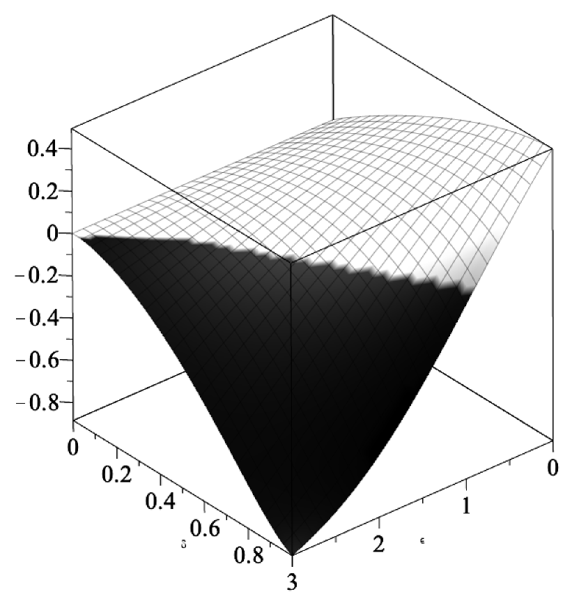
(a)

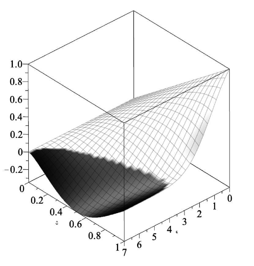
(b)

Figure 1: (1(a)) $g(\epsilon,\delta)$. For the points $(\epsilon,\delta)$ where this quantity is negative, indicated by dark gray, using $\sigma=s(\epsilon,\delta,\Delta)$ violates the sufficient condition (7). (1(b)) $d(\epsilon,\delta)$. Where values are negative, indicated by dark gray, using $\sigma=s(\epsilon,\delta,\Delta)$ violates condition (11) for $(\epsilon,\delta)$-differential privacy.

However, as Balle et al. [2] point out, violating (7) is is not the same as violating $(\epsilon,\delta)$-differential privacy. They show that $(\epsilon,\delta)$-differential privacy is achieved if and only if

$$\Phi\left(\frac{\Delta}{2\sigma}-\frac{\epsilon\sigma}{\Delta}\right)-e^{\epsilon}\Phi\left(-\frac{\Delta}{2\sigma}-\frac{\epsilon\sigma}{\Delta}\right)\leq\delta.$$ (11)

They do not provide a closed form bound based on (11) but provide a numerical algorithm to compute the smallest $\sigma>0$ for which the above holds.

Substituting $s(\epsilon,\delta,\Delta)$ for $\sigma$ in the left side of (11), and subtracting this from $\delta$ yields

$$d(\epsilon,\delta)=\delta-\left(\Phi(-v(s(\epsilon,\delta,\Delta),2))-e^{\epsilon}\Phi(-v(s(\epsilon,\delta,\Delta),-2))\right),$$

which does not depend on $\Delta$. Analogous to $g$ above, the sign of $d$ determines whether (11) and $(\epsilon,\delta)$-differential privacy is violated. A plot of $d(\epsilon,\delta)$ can be seen in Figure 1(b). Negative values indicate failure to be $(\epsilon,\delta)$-differential privacy. The plot suggests that even if the inequality of the standard bound (1) is strict, it is safe to consider it non-strict for $\epsilon\in(0,1)$. What the plot also shows, is that the standard bound does not yield $(\epsilon,\delta)$-differential privacy for all $\epsilon>0$.

5 Comparing the two bounds

The standard bound and our bound differ in both being based on different conditions and how closed form bounds are produced. Specifically, (7) and via the Cramér–Chernoff style tail bound $\Pr(|Z|>x)\leq 2\phi(x)/x$, and (5) and via closed form bound of the inverse error function leading to Lemma 4, respectively.

We now compare the two bounds for the common interval $\epsilon\in(0,1)$.

The ratio of the standard bound (1) and our bound (9) is

$$r(\epsilon,\delta)=\frac{2\sqrt{\log\left(\frac{5}{4\delta}\right)}}{\sqrt{a\log\left(\frac{1}{4\delta\left(1-\delta\right)}\right)+\epsilon}+s\sqrt{a\log\left(\frac{1}{4\delta\left(1-\delta\right)}\right)}}$$ (12)

A value for $r>1$ means that the standard bound is larger than ours. A plot of the ratio $r$ can be seen in Figure 2(a).

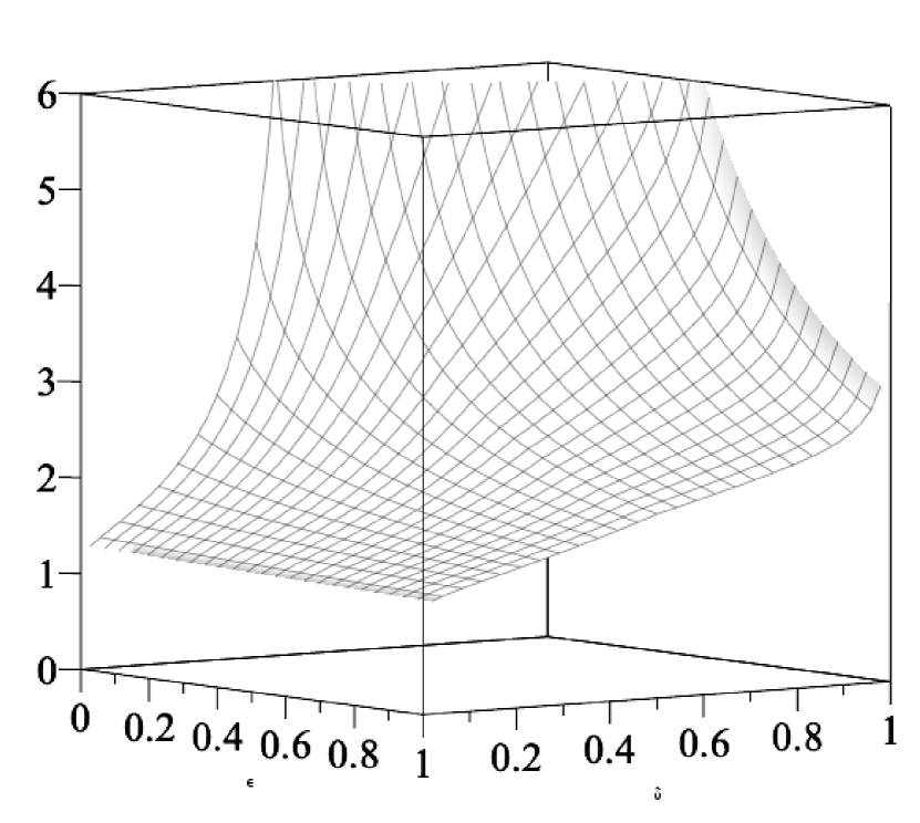
(a)

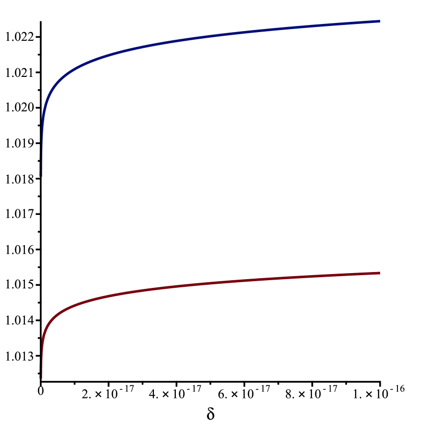
(b)

Figure 2: (2(a)) The ratio $r$ given in (12). Note that all values are at least 1. (2(b)) The functions $\rho_{+}(\delta)=r(0,\delta)$ and $\rho_{-}(\delta)=r(1,\delta)$ giving upper and lower bounds on the ratio $r$ in terms of $\delta$, respectively.

The partial derivative of $r$ in (12) with respect to $\epsilon$ is

$$-\frac{\sqrt{\log\left(\frac{5}{4\delta}\right)}}{\left(\sqrt{a\log\left(\frac{1}{4\delta\left(1-\delta\right)}\right)+\epsilon}+s\sqrt{a\log\left(\frac{1}{4\delta\left(1-\delta\right)}\right)}\right)^{2}\sqrt{a\log\left(\frac{1}{4\delta\left(1-\delta\right)}\right)+\epsilon}}.$$ (13)

This derivative is negative for $\delta>0$ and $\epsilon>0$, meaning that the ratio $r$ decreases as $\epsilon$ increases. It can also be shown that partial derivative of $r$ with respect to $\delta$ is $O(\frac{1}{\delta})$.

We now look at what happens for small $\delta\leq 1/2$. Inspecting $r$, we see that as $\epsilon\to 0$ we get that $r\to\rho_{+}(\delta)$ where

$$\rho_{+}(\delta)=\frac{\sqrt{\log\left(\frac{5}{4\delta}\right)}}{\sqrt{\log\left(\frac{1}{4\delta\left(1-\delta\right)}\right)}},$$

and as $\epsilon\to 1$ we get that $r\to\rho_{-}(\delta)$ where

$$\rho_{-}(\delta)=\frac{2\sqrt{\log\left(\frac{5}{4\delta}\right)}}{\sqrt{\log\left(\frac{1}{4\delta\left(1-\delta\right)}\right)+1}+\sqrt{\log\left(\frac{1}{4\delta\left(1-\delta\right)}\right)}}.$$

Since $r$ is decreasing in $\epsilon$, the functions $\rho_{+}(\delta)$ and $\rho_{-}(\delta)$ provide upper and lower bounds on $r$ for a given value of $\delta\leq 1/2$. Both these functions are increasing in $0<\delta\leq 1/2$ and as $\delta\to 0$ both go towards 1. A plot of $\rho_{+}$ and $\rho_{-}$ for $\delta\leq 10^{-16}$ can be seen in Figure 2(b). As $\rho_{+}(10^{-16})<1.023$, we see that for small $\delta$, the ratio $r$ is not that big. In other words, while our bound (9) is better than the standard bound, it is only slightly better for $\delta$ that can be considered small.

6 Discussion

Simple closed form bounds can be implemented using simple algorithms with low implementation and computational complexity. The benefit of this is a lower potential for errors, as well as decreasing power consumption in low power devices whenever the alternative is using iterative numerical algorithms to compute analytical solutions. Furthermore, closed form relationships are useful in the analysis of processes where privacy mechanisms are components or are applied multiple times.

While our bound is better than the standard bound wherever this is defined, our analysis suggests that for $\delta$ that are small enough to be considered relevant, the improvement is limited. Therefore, we suggest that the main advantage of our bound is that it is valid for all $\epsilon>0$ and that it can be used as a drop in for the standard bound without much difficulty even though it is slightly more complex.

We believe that the condition for $(\epsilon,\delta)$-differential privacy in Lemma 2 is of independent interest as we are able to derive the standard condition for $\epsilon$-differential privacy in the case of Laplace noise.

Our bound (9) is based on the sufficient condition (5). As Balle et al. [2] demonstrate, the optimal $\sigma$ can be gotten through numerically optimizing the sufficient and necessary condition (11). A question we leave unaddressed for now is whether suitable closed form bounds on $\Phi$ can be substituted into (11) to find an even better closed form bound on $\sigma$.

References

- [1] Martín Abadi et al. “Deep Learning with Differential Privacy” In Proceedings of the 2016 ACM SIGSAC Conference on Computer and Communications Security - CCS’16, 2016, pp. 308–318 DOI: 10.1145/2976749.2978318
- [2] Borja Balle and Yu-Xiang Wang “Improving the Gaussian Mechanism for Differential Privacy: Analytical Calibration and Optimal Denoising” 80, Proceedings of Machine Learning Research Stockholmsmässan, Stockholm Sweden: PMLR, 2018, pp. 394–403 URL: http://proceedings.mlr.press/v80/balle18a.html
- [3] Cynthia Dwork and Aaron Roth “The Algorithmic Foundations of Differential Privacy” In Foundations and Trends® in Theoretical Computer Science 9.3–4, 2014, pp. 211–407 DOI: 10.1561/0400000042
- [4] Cynthia Dwork, Frank McSherry, Kobbi Nissim and Adam Smith “Calibrating Noise to Sensitivity in Private Data Analysis” In Proceedings of the Conference on Theory of Cryptography, 2006 DOI: 10.1007/11681878_14
- [5] Cynthia Dwork et al. “Our Data, Ourselves: Privacy Via Distributed Noise Generation” In Advances in Cryptology (EUROCRYPT 2006) 4004 Saint Petersburg, Russia: Springer Verlag, 2006, pp. 486–503 URL: https://www.microsoft.com/en-us/research/publication/our-data-ourselves-privacy-via-distributed-noise-generation/
- [6] P. Kairouz, S. Oh and P. Viswanath “The Composition Theorem for Differential Privacy” In IEEE Transactions on Information Theory 63.6, 2017, pp. 4037–4049
- [7] J. Le Ny and G.. Pappas “Differentially Private Filtering” In IEEE Transactions on Automatic Control 59.2, 2014, pp. 341–354 DOI: 10.1109/TAC.2013.2283096
- [8] Frank McSherry “How Many Secrets Do You Have?”, 2017 URL: https://github.com/frankmcsherry/blog/blob/master/posts/2017-02-08.md
- [9] F… Olver et al. “NIST Digital Library of Mathematical Functions”, 2020 URL: http://dlmf.nist.gov/
- [10] Adrien Saumard and Jon A. Wellner “Log-Concavity and Strong Log-Concavity: A Review”, 2014 arXiv:1404.5886 [math.ST]
- [11] Yu-Xiang Wang, Borja Balle and Shiva Prasad Kasiviswanathan “Subsampled Renyi Differential Privacy and Analytical Moments Accountant” 89, Proceedings of Machine Learning Research PMLR, 2019, pp. 1226–1235 URL: http://proceedings.mlr.press/v89/wang19b.html