Reliable transition properties from excited-state mean-field calculations
Abstract
Delta-self-consistent field theory (SCF) is a conceptually simple and computationally inexpensive method for finding excited states. Using the maximum overlap method to guide optimization of the excited state, SCF has been shown to predict excitation energies with a level of accuracy that is competitive with, and sometimes better than, that of TDDFT. Here we benchmark SCF on a larger set of molecules than has previously been considered, and, in particular, we examine the performance of SCF in predicting transition dipole moments, the essential quantity for spectral intensities. A potential downfall for SCF transition dipoles is origin dependence induced by the nonorthogonality of SCF ground and excited states. We propose and test the simplest correction for this problem, based on symmetric orthogonalization of the states, and demonstrate its use on bacteriochlorophyll structures sampled from the photosynthetic antenna in purple bacteria.
I Introduction
The matrix element of the electric dipole operator between two quantum states, commonly known as a transition dipole moment , is a crucial quantity in simulating spectra and describing excited-state dynamics of molecular systems. The magnitude of the transition dipole moment defines the strength with which a transition between the two states can couple to the electromagnetic field to absorb (or emit) light, while the dipole-dipole interaction between transition dipole moments provides the simplest model for the coupling between excited states on different chromophores.
An important application of this second property is in describing transport of excitons through a network of chromophores, as is seen in the early stages of photosynthesis, as well as synthetic analogues, such as organic polymer light-emitting diodes Barford (2013) and chromophores hosted on DNA scaffolds.Buckhout-White et al. (2014); Hemmig et al. (2016); Olejko and Bald (2017) These systems are often simulated using a Frenkel exciton Hamiltonian, Tretiak et al. (2000); Jordanides, Scholes, and Fleming (2001); Manzano (2013); Bourne Worster et al. (2019)
| (1) |
whose off-diagonal elements, , are the coulomb interaction between the transition dipole moments of the relevant excitation on each chromophore. The light-harvesting antenna in photosynthetic organisms typically contain large numbers of chromophores, which are, themselves, relatively large conjugated organic molecules. For example, the antenna in purple photosynthetic bacteria consists of 3–10 light-harvesting II (LHII) complexes (and one LHI complex) per reaction centre, Trissl, Law, and Cogdell (1999); Scheuring, Rigaud, and Sturgis (2004) each containing 27 (32) bacteriochlorophyll-a (BChla) chromophores of around 140 atoms.Cherezov et al. (2006); Hu et al. (1997) Furthermore, the transition dipole moment of each chromophore, and hence the coupling elements of the Hamiltonian, fluctuate constantly with the vibrations of the molecules. To capture the full time-dependent Hamiltonian, even approximately, calculation of the transition dipole moments should therefore ideally be computationally cheap, as well as reasonably accurate. Current models of exciton dynamics in these systems rely on parameterising the coupling elements from experiment, Tretiak et al. (2000); Ishizaki and Fleming (2009); Mohseni et al. (2013); Wu et al. (2010); Pullerits, Chachisvilis, and Sundström (1996); Pelzer et al. (2014) or use time-dependent density functional theory (TDDFT) to generate representative transition dipole moments from a small handful of chromophores.Stross et al. (2016); Beljonne et al. (2009) On-the-fly TDDFT has been used in this context for a single LHII complex, Sisto et al. (2017) and the present work forms part of a wider effort to scale and refine the approach reported there.
TDDFT Runge and Gross (1984); Casida (1995); Stratmann, Scuseria, and Frisch (1998) is a widely popular method for obtaining the properties, including transition dipole moments, of excited states. Adamo and Jacquemin (2013); Laurent and Jacquemin (2013) With the right choice of exchange-correlation functional and basis set, it yields good accuracy compared to correlated wavefunction methods such as CC2 Sarkar et al. (2020) and EOM-CCSD Caricato et al. (2011); Laurent and Jacquemin (2013), at a much lower computational cost. In TDDFT, excitation energies emerge as the eigenvalues of the Casida equations.Casida (1995); Furche and Burke (2005)
The transition vectors (which arise as eigenvectors) are expressed in a basis of excitations and corresponding de-excitations. Each one can be reshaped into a transition density matrix, with columns and rows , from which the transition properties of the excited state can easily be calculated. The transition dipole moment, for example, is found by tracing the transition density matrix with the dipole operator .
However, TDDFT is still too costly to perform dynamics calculations involving large numbers of BChla chromophores, and this paper amounts to an investigation into how feasible it would be to use the cheaper SCF method. Crucially SCF is not only simpler for the energy evaluation; the excited-state gradient is also available very cheaply because it can be computed using standard ground-state mean-field gradient theory.
SCF is conceptually simple. Excited states are found by promoting an electron from an occupied orbital in the ground state to one of the unoccupied virtual orbitals. The orbitals are then reoptimised for the excited electron configuration using a normal SCF iterative procedure. Hunt and Goddard (1969); Huzinaga and Arnau (1970, 1971); Morokuma and Iwata (1972); Gilbert, Besley, and Gill (2008) Unlike TDDFT, therefore, SCF produces a distinct set of molecular orbitals for the excited state. The transition dipole moment can be calculated as a matrix element between the ground-state and excited determinants.
Initial attempts to locate excited states via an SCF procedure rigidly maintained the orthogonality of the ground and excited states by relaxing the excited state particle (and hole) orbitals within the ground-state virtual space Hunt and Goddard (1969); Huzinaga and Arnau (1970) (or respectively in the virtual and occupied spacesMorokuma and Iwata (1972)). In addition to the convenience of dealing with orthogonal states, these procedures also ensure that relaxing the orbitals does not collapse the excited state wavefunction back down to the ground state. Gilbert et al. later argued that imposing orthogonality in this way led to wavefunctions that were no longer solutions of the full SCF equations and propagated errors and approximations in the ground state. Gilbert, Besley, and Gill (2008) They relaxed the orthogonality condition and searched for high energy solutions to the SCF equations by minimising the energy of the excited state with the added condition that the occupied orbitals at each step of the iterative cycle should overlap as much as possible with their counterparts in the previous iteration. This is known as the maximum overlap method (MOM) and has been shown to be highly successful in finding excited state energies. Gilbert, Besley, and Gill (2008); Barca, Gilbert, and Gill (2018); Hanson-Heine, George, and Besley (2013); Kowalczyk, Yost, and Voorhis (2011) The sizeable test set that we consider in this paper adds to this body of evidence, as well as benchmarking the technique for transition dipole moments.
However, as Gilbert et al. acknowledge in their original paper, allowing non-zero overlap between the ground and excited state can artificially enhance the size of the transition dipole moment (and other transition properties). Nonorthogonality of the states introduces a non-zero transition charge, equal to the size of the overlap. Transition dipole moments calculated from the charged transition density are origin-dependent and therefore have a completely arbitrary magnitude. When the state overlap is very small and the molecule is is positioned with its centre of mass on, or close to, the origin, the error associated with the charged transition density is small, or even negligible. Conversely, if the molecule is positioned far away from the origin, as might be the case for a chromophore located within a larger complex or aggregate centred collectively on the origin, the error associated with this additional charge can quickly escalate. Here we propose and test a simple correction that can be applied to the transition density matrix after the SCF cycle, to restore the orthogonality of the ground and excited state.
II Theory
The transition dipole for an excitation from an initial state to a final state is defined in the standard length gauge as
| (2) |
where is the 3-component dipole operator.
In SCF the states are Slater determinants constructed from spin orbitals with . The orbitals are orthonormal within each state, but, in general, nonorthogonal between states, with inner products . The inner product of the two determinants is the determinant of the orbital inner products:
| (3) |
Following the normal rules for nonorthogonal determinants laid down by Löwdin Löwdin (1955), the transition dipole can be written
| (4) |
where and where denotes matrix adjugate.
Alternatively the value of the transition dipole can be computed from the reduced one-particle transition density matrix:
| (5) |
Here is the one-particle reduced transition density matrix in the atomic-orbital basis, given by
| (6) |
where are the molecular-orbital coefficients for state . For unrestricted calculations the spin summation for the reduced density matrix has additional factors that would be 1 or 0 if a common set of orthonormal orbitals were being used, but here have to be considered explicitly:
| (7) |
where is the analogue of for the spin channel.
As noted above, in SCF, the sets of orbitals and for the ground and excited states are optimised independently, so that the resulting states and are not necessarily orthogonal. As previously recognised in the literature,Gilbert, Besley, and Gill (2008) non-zero overlap between these two states leads to errors in the calculated transition dipole moment. In particular, when states are not exactly orthogonal there is a non-zero transition charge equal to the value of the overlap: . This breaks the origin-independence of the transition dipole moment, making the calculated values virtually meaningless. While the transition charge is sometimes exactly zero (when the ground and excited states are of different symmetries) or very small, any violation of translational invariance is certain to prevent widespread use of transition properties from SCF, and needs to be fixed.
For SCF calculations using Hartree–Fock theory one can clearly proceed by performing nonorthogonal configuration interaction,Thom and Head-Gordon (2009); Malmqvist (1986) not only fixing the transition dipoles but also (presumably) generally improving the quality of the description. On the other hand, for SCF based on DFT, such a procedure is not well defined because the underlying Slater determinants are understood not to be “the” wavefunctions, nor the Hamiltonian to be “the” Hamiltonian.Wu, Cheng, and Van Voorhis (2007) It would be possible to build on the approach developed by Wu et al. in the context of constrained DFT, Wu, Cheng, and Van Voorhis (2007) but that also introduces other choices and approximations.
Here we instead look at the simple expedient of using symmetric orthogonalization to ensure exact orthogonality. Recall that symmetric orthogonalization mixes the two states to make a pair of states that are orthogonal while being as close as possible to the original states, and is defined by the transformation
| (8) |
where and . Based on this transformation, the transition density between the orthogonalized states is given by
| (9) |
where ; this parameter is equal to 1 when , recovering the expected result in this limit. In this work we explore the quality of SCF transition dipoles based on the symmetrically orthogonalized transition density.
III Computational Details
Calculations were performed on a set of 109 small closed-shell molecules containing H, C, N, O and F. These structures are a subset of the benchmark set used in reference,Grimme and Bannwarth (2016) with molecules of 12 atoms or fewer.
Reference energies and transition dipole moments (reported in atomic units) were calculated for the 3 lowest energy singlet excited states of each molecule using EOM-CCSD with an aug-cc-pVTZ basis set. Dunning (1989); Prascher et al. (2011); Kendall, Dunning, and Harrison (1992) The same quantities were also calculated for the 6 lowest energy singlet excited states using TDDFT with the CAM-B3LYP functional Yanai, Tew, and Handy (2004) and aug-cc-pVTZ basis set. CAM-B3LYP has consistently been shown to perform well for prediction of the optical properties of both small molecules Caricato et al. (2011); Sarkar et al. (2020) and a large number of conjugated chromophores of various sizes. Grabarek and Andruniów (2019); Beerepoot et al. (2018); Robinson (2018)
Both EOM-CCSD and TDDFT calculations were performed using Gaussian 16.Frisch et al. (2016) Excited states were cross-referenced between the two methods using the symmetry labels provided by Gaussian. In a small number of cases, the symmetry labelling was unsuccessful or defaulted to a different choice (non-abelian or highest order abelian) of point group between the two methods. In these cases, the excited states were matched by hand based on descent in symmetry and their composition, energy, and transition dipole moment. A full list of symmetries and indices of the selected transitions can be found in the supplementary material.
These data were used to benchmark the performance of SCF in predicting transition properties, both with and without the symmetric orthogonalization correction proposed in equation 9. SCF calculations were performed in the Entos Qcore package,EntosInc. (2 17) with the CAM-B3LYP functional and aug-cc-pVTZ basis set.
We investigated only the HOMO-LUMO singlet transition. Using SCF, we calculated the properties of the state corresponding to the spin-conserving excitation of a HOMO electron into the lowest energy virtual orbital. This does not correspond to a true singlet excitation, which would contain a superposition of and excitations. The spin-purification formula,
| (10) |
was applied to more accurately estimate the true singlet excitation energy. Ziegler, Rauk, and Baerends (1977); Kowalczyk et al. (2013); Hait and Head-Gordon (2020) However, this correction is applied at the end of the SCF cycle and does not affect the composition of the molecular orbitals, which are used to calculate the transition dipole moment. Hait and Head-Gordon (2020)
Since SCF uses a variational principle to optimise the excited state orbitals, a known weakness is that the calculation can converge on the ground state rather than the desired excited state. In most cases, this can be prevented using MOM Gilbert, Besley, and Gill (2008), which selects orbitals to be occupied based on maximum overlap with each occupied molecular orbital in the previous iteration. This stops the orbitals from changing significantly in any particular step of the optimization and helps stabilize the calculation around the excited state stationary points, rather than the global minimum (ground state). However, in a small number of cases, additional help was needed to converge the SCF cycle to the correct excited state. There are a number of well-established techniques to address this issue. We used a combination of Fock-damping, modifying the direct inversion of iterative subspace (DIIS) protocol, Pulay (1980, 1982); Hamilton and Pulay (1985) and starting from an initial guess corresponding to excitation of half an electron.
The properties of the SCF transition were compared to those of the TDDFT transition with the largest coefficient for HOMO-LUMO excitation (based on the orbital indexing in the TDDFT calculation), along with the corresponding EOM-CC transition. For a few molecules this was not an appropriate comparison to make, either because of a reordering of orbitals with very similar energies or because there was no single state dominated by the HOMO-LUMO transition. In these cases, we either selected the correct TDDFT transition by hand or calculated the SCF transition corresponding to the lowest energy TDDFT transition. Full details of these choices can be found in the supplementary material.
IV Results
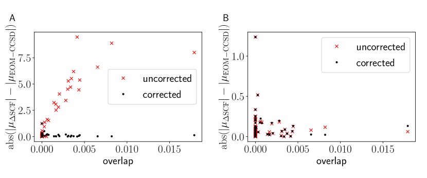
First, we test the effect of applying the symmetric orthogonalization correction, proposed above, to overlapping ground and excited states. Figure 1 shows the error relative to EOM-CCSD in the magnitude of the transition dipole moment, as a function of the ground-excited state overlap for each molecule in the test set using SCF with or without the correction. In panel A, the coordinates of the entire molecule have been translated by 100 Å in each cartesian direction. Physical properties like excitation energy and transition dipole moment should be invariant under this translation; but when there is non-zero overlap between the ground and excited state, the calculation of the transition dipole moment becomes origin-dependent and this coordinate shift introduces an error into the calculated values of .
Although the ground-excited state overlaps are small () for every molecule in the test set, when the molecule is displaced far away from the origin, it is sufficient to produce highly unphysical transition dipoles. Using the symmetric orthogonalization correction, the origin dependence is completely removed and these errors do not arise.
An important consideration is whether applying the correction degrades the accuracy of the SCF calculation in any way. This is difficult to see, since the origin-dependence of the the uncorrected transition dipole moments means that they cannot be taken as a reliable indication of the ‘correct’ SCF transition dipole. However, we note that, by construction, the amount of ground and excited state dipole that are mixed into the transition density (the amount that the correction ‘changes the answer’) scales roughly linearly with the size of the overlap for small overlaps. When the overlap is zero (and the uncorrected SCF transition dipole is therefore already ‘correct’), the symmetric orthogonalization procedure does not change the states, transition density or transition dipole at all. At the largest overlaps present in this test set, the change in the transition dipole that comes from applying the symmetric orthogonalization correction is still very small, as illustrated in panel B of Figure 1.
Note that we do not attach any significance to whether the corrected or uncorrected transition dipole magnitude is closer to the reference value since the uncorrected magnitude can be made to have any value by shifting the coordinates of the molecule. The molecules in this test set are small, with average atomic positions (not center of mass) defining the origin, so we do not expect the uncorrected transition dipole moments to be wildly wrong. However, even shifting the molecule so that its centre-of-mass lies on the origin is sufficient to account for the difference in values seen on the right-hand side of Figure 1. For the larger molecules in the test set, the transition dipole may not span the whole molecule and the concept of the ‘correct’ position or transition dipole for the molecule becomes even less clear.
For the remainder of this paper, the symmetric orthogonalization correction will be applied for all reported SCF transition dipoles.
Figure 2 compares the excitation energy of each molecule calculated using TDDFT and SCF with the value predicted by EOM-CCSD. The energies predicted by SCF are at least as accurate as those predicted using TDDFT, if not slightly more so. TDDFT with CAM-B3LYP has a tendency to slightly underpredict the excitation energy, which is slightly less pronounced in SCF. The exception is one very noticeable outlier, highlighted with a circle in figure 2.
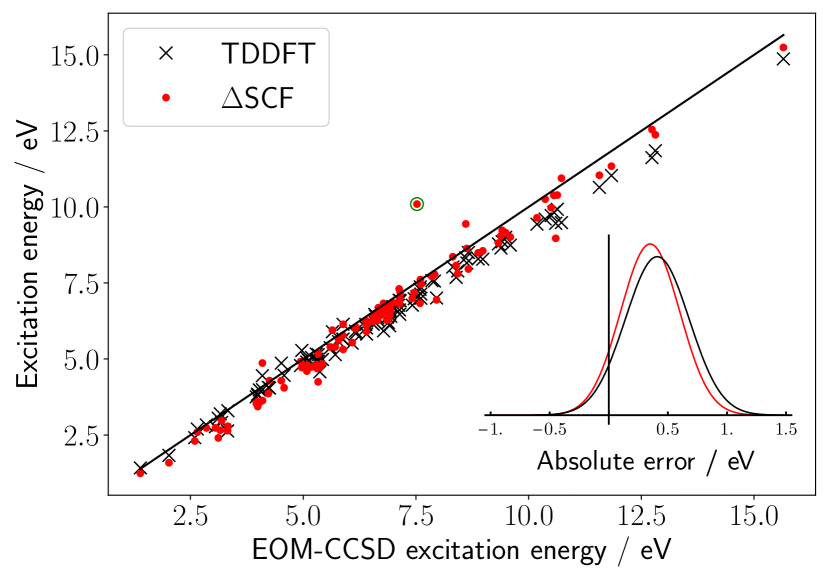
This outlier is a perpendicular ethene dimer, and it serves to illustrate a key situation where SCF may not be an appropriate choice of method. The two highest occupied molecular orbitals in the ground state of the ethene dimer are degenerate, representing the -bonding orbital on each monomer. The two lowest unoccupied molecular orbitals are similarly very close in energy and are in-phase and out-of-phase combinations of the -antibonding orbitals on each molecule. Both EOM-CCSD and TDDFT predict that the two lowest energy excitations of the ethene dimer are degenerate linear combinations of the local excitations with an excitation energy of 7.5 eV and transition dipole moments in the and directions (the principal axis being ). SCF, by construction, cannot capture the mixed nature of these excitations, and instead predicts a excitations with energies around 7 and 10 eV (shown) and transition dipoles in the plane.
Excluding the outlier, the mean error in the SCF excitation energies compared to EOM-CCSD is 0.35, with a standard deviation of 0.25 (table 1). For TDDFT, the mean error is 0.41, with a standard deviation of 0.27. For excitation energies, SCF is therefore clearly worth considering as a cheap and accurate alternative to TDDFT. This is in good agreement with earlier studies benchmarking SCF excitation energies for large organic dyes.Kowalczyk, Yost, and Voorhis (2011); Terranova and Bowler (2013)
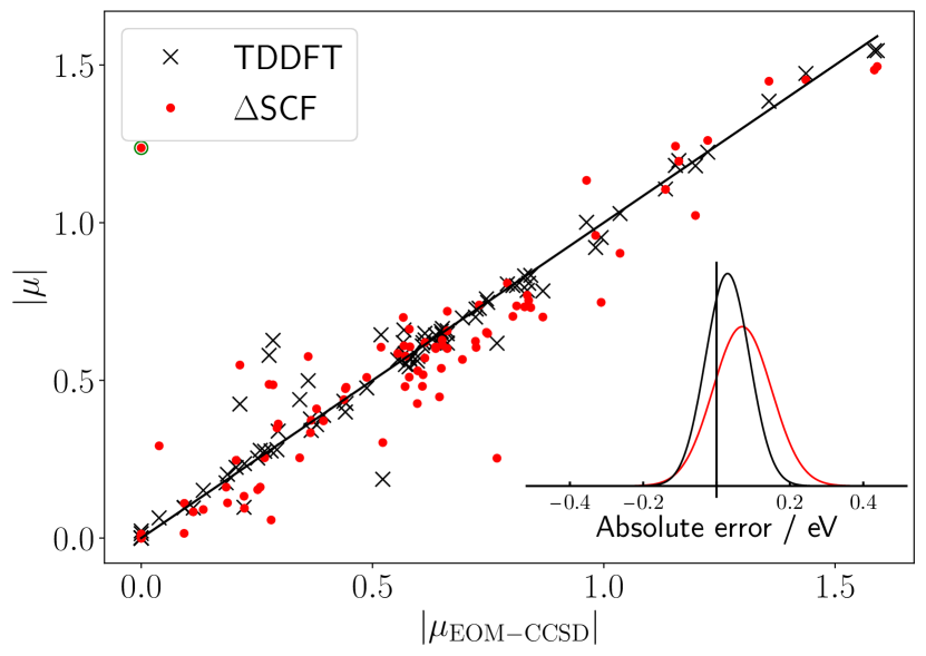
Figure 3 makes the same comparison for . By eye, SCF produces slightly more scatter around the EOM-CCSD reference than TDDFT but has a broadly similar accuracy. This is borne out in a more detailed numerical analysis. The mean error in for SCF compared to EOM-CCSD is 0.07, with a standard deviation of 0.08 (table 1). For TDDFT, the mean error is 0.03, with a standard deviation of 0.06.
There is, again, a single obvious outlier where SCF apparently performs far worse than TDDFT. This outlier corresponds to a stretched version of the benzene molecule. Like the ethene dimer described above, the lowest energy excitation of this structure is a roughly equal mix of HOMO to LUMO and HOMO1 to LUMO+1 transitions. In this case, however, both HOMO and HOMO1 and LUMO and LUMO+1 are exactly degenerate and this creates some flexibility in the definition of the transition and its dipole moment. The transition dipole moment found by SCF agrees very well with that for an excitation that is an equal mix of HOMO to LUMO+1 and HOMO1 to LUMO, which, given the degeneracy of the states, is an equally valid choice. This outlier should therefore be viewed not as a failure of SCF but as a reminder that there isn’t one correct transition dipole moment when degenerate states are involved.
This test set contains two other structures for benzene, with slightly different bond lengths. For these variations, coupled cluster and TDDFT find nearly pure, degenerate HOMO to LUMO and HOMO1 to LUMO+1 transitions, for which SCF predicts very accurate transition dipoles.
Having established the performance of SCF vs. TDDFT, we move on to look at the performance of SCF in calculating the transition properties of the 27 BChla in the LHII complex of purple bacteria. We take the structures of the chromophores from a single snapshot of the molecular dynamics simulation by Stross et al. Stross et al. (2016) This chromophore is too large to treat with EOM-CCSD, so we use TDDFT as our reference, bearing in mind its performance on the test set of smaller molecules. We use the PBE0 functional Adamo and Barone (1999); Perdew, Burke, and Ernzerhof (1996) and Def2-SVP basis set Weigend and Ahlrichs (2005), in line with Ref. 18.
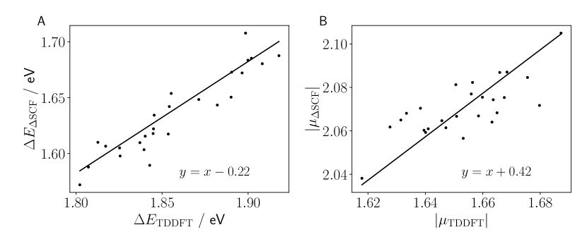
As shown in Figure 2, the excitation energies calculated using SCF correlate extremely well with those predicted by TDDFT and lie well within the range of error of TDDFT. This suggests both that the SCF excitation energies are accurate and that small variations in the energy between the different chromophores are physically meaningful.
By contrast, there is a significant difference between the magnitude of the transition dipoles predicted by TDDFT and SCF, with SCF predicting magnitudes that are, on average, 0.42 a.u. larger. This is larger than the average error expected for TDDFT and SCF compared to EOM-CCSD but within the full range of errors observed for the test set of small molecules. We note that the difference between TDDFT and SCF will have contributions from the error in both methods and it is not clear from figure 4 which will be the largest contribution. However, while it appears that the error in the SCF transition dipole moment is towards the higher end of what we might expect, it is reassuring that the values remain well-correlated with those from TDDFT. This suggests that SCF could be used to create a valid pictures of how the transition dipoles of each chromophore change over the course of a molecular dynamics simulation.
One chromophore is missing from figure 4, as the SCF calculation collapsed back to the ground state. This is a hazard of the SCF method, and we plan to keep working on robustness, including for example by implementing the initial maximum overlap methodBarca, Gilbert, and Gill (2018) (IMOM) based on orbitals from an initial averaged calculation.
V Discussion
We have benchmarked the excitation energies and transition dipole magnitudes predicted by SCF for a large set of small organic molecules. In line with previous work on larger, organic chromophores, we have shown that SCF predicts excitation energies with a very similar accuracy to TDDFT, compared to a highly accurate EOM-CCSD reference. TDDFT still outperforms SCF in predicting the magnitudes of transition dipoles but the error in the SCF predictions are sufficiently small that it can still be considered a useful alternative when TDDFT is too computationally demanding or when speed is of greater importance than higher precision. In contrast to earlier studies, we have focused on testing a large number of different molecules, rather than a range of functionals and basis sets.
A potential downside of many excited state SCF methods, including the MOM, used here, is that the excited state molecular orbitals are optimised independently of the ground state orbitals and there is consequently no guarantee that the ground and excited state will be orthogonal. In their paper first introducing the MOM, Gilbert et al. argue that orthogonality is not an expected property of SCF states, which are approximations of the exact quantum states Gilbert, Besley, and Gill (2008). They further demonstrate that the MOM tends to converge on excited states that only overlap with the ground state by a small amount. Nevertheless, even a small overlap can introduce a problematic origin dependence into the calculation of the transition dipole moment, particularly when the relevant part of the molecule is not close to the origin of the coordinate axis. We have demonstrated that performing a symmetric orthogonalization of the ground and excited states produced by the SCF optimization is a simple way to remove these small overlaps without introducing error into the calculation of the excitation energy or significantly changing the identity of the states. We have demonstrated the use of this correction in the context of simulating photosynthetic antenna complexes, which consist of multiple chromophores arranged into a larger aggregate structure. In a molecular dynamics simulation, for example, these complexes would typically be centred globally on the origin, with each individual chromophore therefore being displaced well away from the origin. Applying our simple correction to the transition density matrix is significantly more straightforward than recentering every single chromophore (whilst also keeping track of its original position relative to all the other chromophores). We anticipate that this trick will be extremely useful in the application of cheaper excited-state SCF methods to biological systems.
We have seen that the greatest potential for SCF to fail occurs when the transition of interest is highly mixed in nature. This is not surprising, since SCF is constructed to deal with transitions between a single occupied ground state orbital and a single (relaxed) virtual orbital. Highly mixed transitions usually occur when there are low-lying virtual orbitals of the same symmetry with very similar energies. By calculating the energies and symmetries of the molecular orbitals (programs like Gaussian provide an option to do this automatically), a simple inspection would identify molecules with a greater risk of highly mixed transitions, helping to determine whether SCF could be appropriately used. Furthermore, large molecules, for which TDDFT may become prohibitively expensive, typically have much lower symmetry than the small molecules considered here, greatly reducing the chances that near-degenerate molecular orbitals of the same symmetry will exist.
Looking forward, we suggest that there is potential to further improve the ability of SCF to predict accurate transition dipole moments. Previous work by Kowalczyk et al. Kowalczyk, Yost, and Voorhis (2011) demonstrates that much of the error in SCF excitation energies arises from spin contamination and that this effect is more pronounced for functionals with a smaller amount of exact exchange. While excitation energies can be, at least partially, corrected for spin contamination using the spin purification formula described above, this correction does not extend to the molecular orbitals used to calculate the transition density, and related properties. We hypothesise that the performance of SCF for transition dipoles could be improved by incorporating spin purification into the calculation of the molecular orbitals. This could be done, for example, by minimising the spin-purified energy in the SCF cycle, rather than applying the correction at the end of the energy calculation. Trialling such a procedure is, however, beyond the scope of the current study.
| Error in | Error in | |||
|---|---|---|---|---|
| SCF | TDDFT | SCF | TDDFT | |
| mean | 0.35 | 0.41 | 0.07 | 0.03 |
| std. dev. | 0.25 | 0.27 | 0.08 | 0.06 |
| min. | 0.01 | 0.02 | 0.00 | 0.00 |
| max. | 1.63 | 1.24 | 0.52 | 0.34 |
Acknowledgements.
We gratefully acknowledge the funding agencies that supported this work: O.F. is funded by the U.S. Department of Energy (DE-FOA-0001912). S.B.W. is supported by a research fellowship from the Royal Commission for the Exhibition of 1851References
- Barford (2013) W. Barford, “Excitons in conjugated polymers: a tale of two particles.” The Journal of Physical Chemistry A 117, 2665–71 (2013).
- Buckhout-White et al. (2014) S. Buckhout-White, C. M. Spillmann, W. R. Algar, A. Khachatrian, J. S. Melinger, E. R. Goldman, M. G. Ancona, and I. L. Medintz, “Assembling programmable FRET-based photonic networks using designer DNA scaffolds,” Nature Communications 5, 5615 (2014).
- Hemmig et al. (2016) E. A. Hemmig, C. Creatore, B. Wunsch, L. Hecker, P. Mair, M. A. Parker, S. Emmott, P. Tinnefeld, U. F. Keyser, and A. W. Chin, “Programming Light-Harvesting Efficiency Using DNA Origami,” Nano Letters 16, 2369–2374 (2016).
- Olejko and Bald (2017) L. Olejko and I. Bald, “FRET efficiency and antenna effect in multi-color DNA origami-based light harvesting systems,” RSC Adv. 7, 23924–23934 (2017).
- Tretiak et al. (2000) S. Tretiak, C. Middleton, V. Chernyak, and S. Mukamel, “Exciton Hamiltonian for the Bacteriochlorophyll System in the LH2 Antenna Complex of Purple Bacteria,” Journal of Physical Chemistry B 104, 4519–4528 (2000).
- Jordanides, Scholes, and Fleming (2001) X. J. Jordanides, G. D. Scholes, and G. R. Fleming, “The Mechanism of Energy Transfer in the Bacterial Photosynthetic Reaction Center,” The Journal of Physical Chemistry B 105, 1652–1669 (2001).
- Manzano (2013) D. Manzano, “Quantum Transport in Networks and Photosynthetic Complexes at the Steady State,” PLoS ONE 8, 1–8 (2013).
- Bourne Worster et al. (2019) S. Bourne Worster, C. Stross, F. M. W. C. Vaughan, N. Linden, and F. R. Manby, “Structure and Efficiency in Bacterial Photosynthetic Light Harvesting,” The Journal of Physical Chemistry Letters 10, 7383–7390 (2019).
- Trissl, Law, and Cogdell (1999) H. W. Trissl, C. J. Law, and R. J. Cogdell, “Uphill energy transfer in LH2-containing purple bacteria at room temperature,” Biochimica et Biophysica Acta - Bioenergetics 1412, 149–172 (1999).
- Scheuring, Rigaud, and Sturgis (2004) S. Scheuring, J. L. Rigaud, and J. N. Sturgis, “Variable LH2 stoichiometry and core clustering in native membranes of Rhodospirillum photometricum,” EMBO Journal 23, 4127–4133 (2004).
- Cherezov et al. (2006) V. Cherezov, J. Clogston, M. Z. Papiz, and M. Caffrey, “Room to move: Crystallizing membrane proteins in swollen lipidic mesophases,” Journal of Molecular Biology 357, 1605–1618 (2006).
- Hu et al. (1997) X. Hu, T. Ritz, A. Damjanović, and K. Schulten, “Pigment Organization and Transfer of Electronic Excitation in the Photosynthetic Unit of Purple Bacteria,” The Journal of Physical Chemistry B 101, 3854–3871 (1997).
- Ishizaki and Fleming (2009) A. Ishizaki and G. R. Fleming, “Theoretical examination of quantum coherence in a photosynthetic system at physiological temperature,” Proceedings of the National Academy of Sciences 106, 17255–17260 (2009).
- Mohseni et al. (2013) M. Mohseni, A. Shabani, S. Lloyd, Y. Omar, and H. Rabitz, “Geometrical effects on energy transfer in disordered open quantum systems,” Journal of Chemical Physics 138 (2013), 10.1063/1.4807084.
- Wu et al. (2010) J. Wu, F. Liu, Y. Shen, J. Cao, and R. J. Silbey, “Efficient energy transfer in light-harvesting systems, I: Optimal temperature, reorganization energy and spatial-temporal correlations,” New Journal of Physics 12 (2010), 10.1088/1367-2630/12/10/105012.
- Pullerits, Chachisvilis, and Sundström (1996) T. Pullerits, M. Chachisvilis, and V. Sundström, “Exciton Delocalization Length in the B850 Antenna of Rhodobacter sphaeroides,” The Journal of Physical Chemistry 100, 10787–10792 (1996).
- Pelzer et al. (2014) K. M. Pelzer, T. Can, S. K. Gray, D. K. Morr, and G. S. Engel, “Coherent transport and energy flow patterns in photosynthesis under incoherent excitation,” The Journal of Physical Chemistry B 118, 2693–2702 (2014).
- Stross et al. (2016) C. Stross, M. W. Van der Kamp, T. A. A. Oliver, J. N. Harvey, N. Linden, and F. R. Manby, “How Static Disorder Mimics Decoherence in Anisotropy Pump-Probe Experiments on Purple-Bacteria Light Harvesting Complexes,” The Journal of Physical Chemistry B 120, 11449–11463 (2016).
- Beljonne et al. (2009) D. Beljonne, C. Curutchet, G. D. Scholes, and R. J. Silbey, “Beyond förster resonance energy transfer in biological and nanoscale systems,” Journal of Physical Chemistry B 113, 6583–6599 (2009).
- Sisto et al. (2017) A. Sisto, C. Stross, M. W. van der Kamp, M. O’Connor, S. McIntosh-Smith, G. T. Johnson, E. G. Hohenstein, F. R. Manby, D. R. Glowacki, and T. J. Martinez, “Atomistic non-adiabatic dynamics of the LH2 complex with a GPU-accelerated ab initio exciton model,” Physical Chemistry Chemical Physics 19, 14924–14936 (2017).
- Runge and Gross (1984) E. Runge and E. K. U. Gross, “Density-Functional Theory for Time-Dependent Systems,” Physical Review Letters 52, 997–1000 (1984).
- Casida (1995) M. E. Casida, “Time-dependent density-functional response theory for molecules,” Recent advances in density functional methods, part 1. , 1–34 (1995).
- Stratmann, Scuseria, and Frisch (1998) R. E. Stratmann, G. E. Scuseria, and M. J. Frisch, “An efficient implementation of time-dependent density-functional theory for the calculation of excitation energies of large molecules,” Journal of Chemical Physics 109, 8218–8224 (1998).
- Adamo and Jacquemin (2013) C. Adamo and D. Jacquemin, “The calculations of excited-state properties with time-dependent density functional theory,” Chemical Society Reviews 42, 845–856 (2013).
- Laurent and Jacquemin (2013) A. D. Laurent and D. Jacquemin, “TD-DFT benchmarks: A review,” International Journal of Quantum Chemistry 113, 2019–2039 (2013).
- Sarkar et al. (2020) R. Sarkar, M. Boggio-Pasqua, P.-F. Loos, and D. Jacquemin, “Benchmarking TD-DFT and Wave Function Methods for Oscillator Strengths and Excited-State Dipole Moments,” arXiv:2011.13233v1 , 27–30 (2020).
- Caricato et al. (2011) M. Caricato, G. W. Trucks, M. J. Frisch, and K. B. Wiberg, “Oscillator strength: How does TDDFT compare to EOM-CCSD?” Journal of Chemical Theory and Computation 7, 456–466 (2011).
- Furche and Burke (2005) F. Furche and K. Burke, “Chapter 2 Time-Dependent Density Functional Theoryin Quantum Chemistry,” Annual Reports in Computational Chemistry 1, 19–30 (2005).
- Hunt and Goddard (1969) s. W. J. Hunt and W. A. Goddard, “Excited States of H2O using improved virtual orbitals,” Chemical Physics Letters 3, 414–418 (1969).
- Huzinaga and Arnau (1970) S. Huzinaga and C. Arnau, “Virtual orbitals in Hartree-Fock theory,” Physical Review A 1, 1285–1288 (1970).
- Huzinaga and Arnau (1971) S. Huzinaga and C. Arnau, “Virtual orbitals in hartree-fock theory. II,” The Journal of Chemical Physics 54, 1948–1951 (1971).
- Morokuma and Iwata (1972) K. Morokuma and S. Iwata, “Extended Hartree-Fock theory for excited states,” Chemical Physics Letters 16, 192–197 (1972).
- Gilbert, Besley, and Gill (2008) A. T. Gilbert, N. A. Besley, and P. M. Gill, “Self-consistent field calculations of excited states using the maximum overlap method (MOM),” Journal of Physical Chemistry A 112, 13164–13171 (2008).
- Barca, Gilbert, and Gill (2018) G. M. Barca, A. T. Gilbert, and P. M. Gill, “Simple Models for Difficult Electronic Excitations,” Journal of Chemical Theory and Computation 14, 1501–1509 (2018).
- Hanson-Heine, George, and Besley (2013) M. W. Hanson-Heine, M. W. George, and N. A. Besley, “Calculating excited state properties using Kohn-Sham density functional theory,” Journal of Chemical Physics 138 (2013), 10.1063/1.4789813.
- Kowalczyk, Yost, and Voorhis (2011) T. Kowalczyk, S. R. Yost, and T. V. Voorhis, “Assessment of the SCF density functional theory approach for electronic excitations in organic dyes,” Journal of Chemical Physics 134 (2011), 10.1063/1.3530801.
- Löwdin (1955) P.-O. Löwdin, “Quantum Theory of Many-Particle Systems. I. Physical Interpretations by Means of Density Matrices, Natural Spin-Orbitals, and Convergence Problems in the Method of Configurational Interaction,” Physical Review 97, 1474–1489 (1955).
- Thom and Head-Gordon (2009) A. J. Thom and M. Head-Gordon, “Hartree-Fock solutions as a quasidiabatic basis for nonorthogonal configuration interaction,” Journal of Chemical Physics 131, 1–6 (2009).
- Malmqvist (1986) P. . Malmqvist, “Calculation of transition density matrices by nonunitary orbital transformations,” International Journal of Quantum Chemistry 30, 479–494 (1986).
- Wu, Cheng, and Van Voorhis (2007) Q. Wu, C.-L. Cheng, and T. Van Voorhis, “Configuration interaction based on constrained density functional theory: A multireference method,” The Journal of Chemical Physics 127, 164119 (2007).
- Grimme and Bannwarth (2016) S. Grimme and C. Bannwarth, “Ultra-fast computation of electronic spectra for large systems by tight-binding based simplified Tamm-Dancoff approximation (sTDA-xTB),” Journal of Chemical Physics 145 (2016), 10.1063/1.4959605.
- Dunning (1989) T. H. Dunning, “Gaussian basis sets for use in correlated molecular calculations. I. The atoms boron through neon and hydrogen,” The Journal of Chemical Physics 90, 1007–1023 (1989).
- Prascher et al. (2011) B. P. Prascher, D. E. Woon, K. A. Peterson, T. H. Dunning, and A. K. Wilson, “Gaussian basis sets for use in correlated molecular calculations. VII. Valence, core-valence, and scalar relativistic basis sets for Li, Be, Na, and Mg,” Theoretical Chemistry Accounts 128, 69–82 (2011).
- Kendall, Dunning, and Harrison (1992) R. A. Kendall, T. H. Dunning, and R. J. Harrison, “Electron affinities of the first-row atoms revisited. Systematic basis sets and wave functions,” The Journal of Chemical Physics 96, 6796–6806 (1992).
- Yanai, Tew, and Handy (2004) T. Yanai, D. P. Tew, and N. C. Handy, “A new hybrid exchange-correlation functional using the Coulomb-attenuating method (CAM-B3LYP),” Chemical Physics Letters 393, 51–57 (2004).
- Grabarek and Andruniów (2019) D. Grabarek and T. Andruniów, “Assessment of Functionals for TDDFT Calculations of One- and Two-Photon Absorption Properties of Neutral and Anionic Fluorescent Proteins Chromophores,” Journal of Chemical Theory and Computation 15, 490–508 (2019).
- Beerepoot et al. (2018) M. T. Beerepoot, M. M. Alam, J. Bednarska, W. Bartkowiak, K. Ruud, and R. Zaleśny, “Benchmarking the Performance of Exchange-Correlation Functionals for Predicting Two-Photon Absorption Strengths,” Journal of Chemical Theory and Computation 14, 3677–3685 (2018).
- Robinson (2018) D. Robinson, “Comparison of the Transition Dipole Moments Calculated by TDDFT with High Level Wave Function Theory,” Journal of Chemical Theory and Computation 14, 5303–5309 (2018).
- Frisch et al. (2016) M. J. Frisch, G. W. Trucks, H. B. Schlegel, G. E. Scuseria, M. A. Robb, J. R. Cheeseman, G. Scalmani, V. Barone, G. A. Petersson, H. Nakatsuji, X. Li, M. Caricato, A. V. Marenich, J. Bloino, B. G. Janesko, R. Gomperts, B. Mennucci, H. P. Hratchian, J. V. Ortiz, A. F. Izmaylov, J. L. Sonnenberg, D. Williams-Young, F. Ding, F. Lipparini, J. F. Egidi, . Goings, B. Peng, A. Petrone, T. Henderson, D. Ranasinghe, V. G. Zakrzewski, J. Gao, N. Rega, G. Zheng, W. Liang, M. Hada, M. Ehara, K. Toyota, R. Fukuda, J. Hasegawa, M. Ishida, T. Nakajima, Y. Honda, O. Kitao, H. Nakai, T. Vreven, K. Throssell, J. A. Montgomery Jr., J. E. Peralta, F. Ogliaro, M. J. Bearpark, J. J. Heyd, E. N. Brothers, K. N. Kudin, V. N. Staroverov, T. A. Keith, R. Kobayashi, J. Normand, K. Raghavachari, A. P. Rendell, J. C. Burant, S. S. Iyengar, J. Tomasi, M. Cossi, J. M. Millam, M. Klene, C. Adamo, R. Cammi, J. W. Ochterski, R. L. Martin, K. Morokuma, O. Farkas, J. B. Foresman, and D. J. Fox, “Gaussian 16,” (2016).
- EntosInc. (2 17) EntosInc., “Qcore,” URL: https://www.entos.ai (accessed: 2020-12-17).
- Ziegler, Rauk, and Baerends (1977) T. Ziegler, A. Rauk, and E. J. Baerends, “On the calculation of multiplet energies by the hartree-fock-slater method,” Theoretica Chimica Acta 43, 261–271 (1977).
- Kowalczyk et al. (2013) T. Kowalczyk, T. Tsuchimochi, P. T. Chen, L. Top, and T. Van Voorhis, “Excitation energies and Stokes shifts from a restricted open-shell Kohn-Sham approach,” Journal of Chemical Physics 138 (2013), 10.1063/1.4801790.
- Hait and Head-Gordon (2020) D. Hait and M. Head-Gordon, “Excited State Orbital Optimization via Minimizing the Square of the Gradient: General Approach and Application to Singly and Doubly Excited States via Density Functional Theory,” Journal of Chemical Theory and Computation 16, 1699–1710 (2020).
- Pulay (1980) P. Pulay, “Convergence acceleration of iterative sequences. the case of scf iteration,” Chemical Physics Letters 73, 393–398 (1980).
- Pulay (1982) P. Pulay, “Improved SCF convergence acceleration,” Journal of Computational Chemistry 3, 556–560 (1982).
- Hamilton and Pulay (1985) T. P. Hamilton and P. Pulay, “Direct inversion in the iterative subspace (DIIS) optimization of open-shell, excited-state, and small multiconfiguration SCF wave functions,” The Journal of Chemical Physics 84, 5728–5734 (1985).
- Terranova and Bowler (2013) U. Terranova and D. R. Bowler, “ Self-Consistent Field Method for Natural Anthocyanidin Dyes,” Journal of Chemical Theory and Computation 9, 3181–3188 (2013).
- Adamo and Barone (1999) C. Adamo and V. Barone, “Toward reliable density functional methods without adjustable parameters: The PBE0 model,” Journal of Chemical Physics 110, 6158–6170 (1999).
- Perdew, Burke, and Ernzerhof (1996) J. P. Perdew, K. Burke, and M. Ernzerhof, “Generalized gradient approximation made simple,” Physical Review Letters 77, 3865–3868 (1996).
- Weigend and Ahlrichs (2005) F. Weigend and R. Ahlrichs, “Balanced basis sets of split valence, triple zeta valence and quadruple zeta valence quality for H to Rn: Design and assessment of accuracy,” Physical Chemistry Chemical Physics 7, 3297–3305 (2005).