Top and Beauty synergies in SMEFT-fits at present and future colliders

Abstract

We perform global fits within Standard Model Effective Field Theory (SMEFT) combining top-quark pair production processes and decay with $b\rightarrow s$ flavor changing neutral current transitions and $Z\to b\bar{b}$ in three stages: using existing data from the LHC and $B$–factories, using projections for the HL-LHC and Belle II, and studying the additional new physics impact from a future lepton collider. The latter is ideally suited to directly probe $\ell^{+}\ell^{-}\rightarrow t\bar{t}$ transitions. We observe powerful synergies in combining both top and beauty observables as flat directions are removed and more operators can be probed. We find that a future lepton collider significantly enhances this interplay and qualitatively improves global SMEFT fits.

I Introduction

Physics beyond the Standard Model (BSM) has and is being intensively searched for at the Large Hadron Collider (LHC) and predecessor machines. However, despite the large amount of data analyzed, no direct detection of BSM particles has been reported to date. Thus, BSM physics could be feebly interacting only, has signatures not covered by the standard searches, or is simply sufficiently separated from the electroweak scale. The latter scenario opens up a complementary approach to hunt for BSM physics at high energy colliders, in a similar spirit as the high luminosity flavor physics programs in pursuit of the precision frontiers with indirect searches. In this regard, the Standard Model Effective Field Theory (SMEFT) offers both a systematic and model-independent way to parametrize BSM contributions in terms of higher-dimensional operators constructed out of Standard Model (SM) fields and consistent with SM symmetries. At energies below the scale of BSM physics, $\Lambda$, this framework allows to perform global fits which could give hints for signatures of BSM physics in different observables and sectors simultaneously.

In recent years, this approach played a crucial role in the top-quark sector of SMEFT Degrande et al. (2018); Chala et al. (2019); Durieux et al. (2015); Aguilar-Saavedra (2011); D’Hondt et al. (2018); Durieux et al. (2018a); Buckley et al. (2015, 2016); de Beurs et al. (2018); Brown et al. (2019); Barducci et al. (2018); Hartland et al. (2019); Maltoni et al. (2019); Durieux et al. (2019); Neumann and Sullivan (2019); Brivio et al. (2020); Dror et al. (2016). The SMEFT framework also allows the combination of top-quark data with $B$ data Bißmann et al. (2020a); Aoude et al. (2020); Fox et al. (2008); Grzadkowski and Misiak (2008); Drobnak et al. (2012); Brod et al. (2015), which, thanks to different sensitivities, significantly improves constraints on SMEFT coefficients Bißmann et al. (2020a).

In this work, we extend previous works and analyze sensitivities to semileptonic four-fermion operators. The reason for doing so goes way beyond of making the fit more model-independent: Firstly, semileptonic four-fermion operators are presently of high interest as they are the agents of the flavor anomalies, hints of a breakdown of the SM in semileptonic $b\to s$ decay data Bifani et al. (2019). Secondly, these operators provide contact interactions of top quarks and leptons, which could be studied ideally at future lepton colliders, e.g. ILC Amjad et al. (2015, 2013), CLIC Abramowicz et al. (2019) or FCC Abada et al. (2019), as discussed in Refs. Kane et al. (1992); Atwood and Soni (1992); Grzadkowski et al. (1997); Brzezinski et al. (1999); Boos et al. (2000); Jezabek et al. (2000); Grzadkowski and Hioki (2000); Janot (2015); Röntsch and Schulze (2015); Khiem et al. (2015); Englert and Russell (2017); Durieux et al. (2018b); Cao and Yan (2015). We intend to specifically work out and detail the interplay of constraints for operators with gauge bosons, that is, covariant derivatives in the SMEFT language, and four fermion operators in top-pair production processes, $Z\to b\bar{b}$ and $b\to s$ transitions for three stages: today, combining existing LHC, $Zbb$ and $B$-factory data, near future, adding projections from HL-LHC Atl (2019) and Belle II Altmannshofer et al. (2019), and the far future, putting all together with lepton collider input, for the concrete example of CLIC Abramowicz et al. (2019); we investigate how a future lepton collider impacts constraints and opens up new directions for testing BSM physics precisely.

This work is organized as follows: In Sec. II we introduce the dimension-six SMEFT operators considered in this work and the low-energy effective field theories (EFTs) employed to compute SM and BSM contributions to $B$ observables. We also present the matching between SMEFT and weak effective theory (WET) and highlight how $SU(2)_{L}$ invariance of the SMEFT Lagrangian allows to relate top-quark physics and $b\rightarrow s$ flavor-changing neutral currents (FCNCs). In Sec. III we discuss the sensitivity of different observables to the various effective operators considered. Fits to present top-quark, $Zbb$, and $B$ data are presented in Sec. IV. We analyze how the complementary sensitivity of the observables from top-quark, $Zbb$, and $B$ sectors improves constraints on the SMEFT coefficients. In Sec. V we consider different future scenarios, and detail on the question how measurements at a future lepton collider can provide additional information on SMEFT coefficients. In Sec. VI we conclude. Additional information is provided in several appendices.

II Effective theory setup

In this section we give the requisite EFT setup to describe BSM contributions to top-quark and beauty observables. We introduce the SMEFT Lagrangian in Sec. II.1, and identify the effective operators contributing to interactions of third-generation quarks. Consequences for FCNCs that arise from flavor mixing are worked out in Sec. II.2, where we also highlight the complementarity between contributions from up-type and down-type quarks. The matching conditions for $B$ observables in the low energy effective Lagrangian in terms of SMEFT coefficients are detailed in Sec. II.3.

II.1 SMEFT dimension-six operators

At energies sufficiently below the scale of new physics, $\Lambda$, the effects of new interactions and BSM particles can be described by a series of higher-dimensional effective operators with mass dimension $d>4$ Weinberg (1979); Buchmuller and Wyler (1986). These operators are built out of SM fields and respect the symmetries of the SM. The SMEFT Lagrangian $\mathcal{L}_{\text{SMEFT}}$ is obtained by adding these $d$-dimensional operators $O_{i}^{(d)}$ together with corresponding Wilson coefficients $C_{i}^{(d)}$ to the SM Lagrangian $\mathcal{L}_{\text{SM}}$. The $C_{i}^{(d)}$ encode the BSM couplings and, in order to be dimensionless, require a factor of $\Lambda^{4-d}$. The leading SMEFT contributions arise at dimension six:

$$\mathcal{L}_{\textmd{SMEFT}}=\mathcal{L}_{\textmd{SM}}+\sum_{i}\frac{C^{(6)}_{i}}{\Lambda^{2}}O_{i}^{(6)}+\mathcal{O}\left(\Lambda^{-4}\right)\,.$$ (1)

Contributions from odd-dimensional operators lead to lepton- and baryon-number violation Degrande et al. (2013); Kobach (2016) and are neglected in this work. In the following, we employ the Warsaw basis Grzadkowski et al. (2010) of dimension-six operators, and consider operators with gauge bosons

$$\begin{aligned} &O_{\varphi q}^{(1)}=\left(\varphi^{\dagger}i\overleftrightarrow{D}_{\mu}\varphi\right)\left(\bar{q}_{L}\gamma^{\mu}q_{L}\right)\,,\quad O_{\varphi q}^{(3)}=\left(\varphi^{\dagger}i\overleftrightarrow{D}_{\mu}^{I}\varphi\right)\left(\bar{q}_{L}\tau^{I}\gamma^{\mu}q_{L}\right)\,,\\ &O_{uB}=\left(\bar{q}_{L}\sigma^{\mu\nu}u_{R}\right)\tilde{\varphi}B_{\mu\nu}\,,\quad O_{uW}=\left(\bar{q}_{L}\sigma^{\mu\nu}\tau^{I}u_{R}\right)\tilde{\varphi}W_{\mu\nu}^{I}\,,\quad O_{uG}=\left(\bar{q}_{L}\sigma^{\mu\nu}T^{A}u_{R}\right)\tilde{\varphi}G_{\mu\nu}^{A}\,,\\ &O_{\varphi u}=\left(\varphi^{\dagger}i\overleftrightarrow{D}_{\mu}\varphi\right)\left(\bar{u}_{R}\gamma^{\mu}u_{R}\right)\,,\quad\end{aligned}$$ (2)

and semileptonic four-fermion operators

$$\begin{aligned} &O_{lq}^{(1)}=\left(\bar{l}_{L}\gamma_{\mu}l_{L}\right)\left(\bar{q}_{L}\gamma^{\mu}q_{L}\right)\,,\quad O_{lq}^{(3)}=\left(\bar{l}_{L}\gamma_{\mu}\tau^{I}l_{L}\right)\left(\bar{q}_{L}\gamma^{\mu}\tau^{I}q_{L}\right)\,,\quad O_{qe}=\left(\bar{q}_{L}\gamma_{\mu}q_{L}\right)\left(\bar{e}_{R}\gamma^{\mu}e_{R}\right)\,,\\ &O_{eu}=\left(\bar{e}_{R}\gamma_{\mu}e_{R}\right)\left(\bar{u}_{R}\gamma^{\mu}u_{R}\right)\,,\quad O_{lu}=\left(\bar{l}_{L}\gamma_{\mu}l_{L}\right)\left(\bar{u}_{R}\gamma^{\mu}u_{R}\right)\,.\end{aligned}$$ (3)

Here, $q_{L}$, $l_{L}$ are the quark and lepton $SU(2)_{L}$ doublets, and $u_{R}$, $e_{R}$ the up-type quark and charged lepton $SU(2)_{L}$ singlets, respectively. Flavor indices that exist for each SM fermion field are suppressed here for brevity but will be discussed in Sec. II.2. With $B_{\mu\nu}$, $W^{I}_{\mu\nu}$ and $G^{A}_{\mu\nu}$ we denote the gauge field strength tensors of $U(1)_{Y}$, $SU(2)_{L}$ and $SU(3)_{C}$, respectively. $T^{A}=\lambda^{A}/2$ and $\tau^{I}/2$ are the generators of $SU(3)_{C}$ and $SU(2)_{L}$ in the fundamental representation with $A=1,\dots,8$ and $I=1,2,3$, and $\lambda^{A}$ and $\tau^{I}$ are the Gell–Mann and Pauli matrices, respectively. The SM Higgs doublet is denoted by $\varphi$ with its conjugate given as $\tilde{\varphi}=i\tau^{2}\varphi$, $\left(\varphi^{\dagger}i\overleftrightarrow{D}_{\mu}\varphi\right)=i\varphi^{\dagger}(D_{\mu}\varphi)-i(D_{\mu}\varphi^{\dagger})\varphi$ and $\left(\varphi^{\dagger}i\overleftrightarrow{D}_{\mu}^{I}\varphi\right)=i\varphi^{\dagger}\tau^{I}(D_{\mu}\varphi)-i(D_{\mu}\varphi^{\dagger})\tau^{I}\varphi$.

Further dimension-six operators exist that contribute at subleading order to top-quark observables such as dipole operators $O_{dX}$ with $X=B,W,G$ and right-handed $b$ quarks, with contributions suppressed by $m_{b}/m_{t}$. We neglect those as well as all other SMEFT operators involving right-handed down-type quarks. Scalar and tensor operators $O^{(1/3)}_{lequ}$ are not included in our analysis since these operators do not give any relevant contributions at $\mathcal{O}(\Lambda^{-2})$ for the interactions considered in this work Durieux et al. (2019); Durieux et al. (2018b). Contributions from four-quark operators to $t\bar{t}\gamma$, $t\bar{t}Z$ and $t\bar{t}$ production are neglected as $t\bar{t}$ production at the LHC is dominated by the $gg$ channel Buckley et al. (2016) . In addition we also neglect leptonic dipole operators, i.e., vertex corrections to lepton currents because they are severely constrained by $Z$-precision measurements Zyla et al. (2020).

Note that dipole operators are in general non-hermitian which allows for complex-valued Wilson coefficients. However, the dominant interference terms are proportional only to the real part of the coefficients. For the sake of simplicity, we thus assume all coefficients to be real-valued.

II.2 Flavor and mass basis

The dimension-six operators (2), (3) are given in the flavor basis. In general, quark mass and flavor bases are related by unitary transformations $S^{k}_{L/R}$, $k=u,d$,

$$u_{L/R}^{i}=\left(S^{u}_{L/R}\right)_{ij}u^{\prime j}_{L/R}\,,\quad d_{L/R}^{i}=\left(S^{d}_{L/R}\right)_{ij}d^{\prime j}_{L/R}\,,$$ (4)

where $u^{\prime}$ and $d^{\prime}$ denote up- and down-type quarks in the mass basis, respectively, and $i,j=1,2,3$ are flavor indices. The CKM matrix $V$ is then given as

$$V=\left(S^{u}_{L}\right)^{\dagger}S^{d}_{L}\,.$$ (5)

The rotation matrices of right handed quarks $S_{R}^{u/d}$ can simply be absorbed in the flavor-basis Wilson coefficient $C_{i}$, giving rise to coefficients in the mass basis, denoted by $\hat{C}_{i}$ Aebischer et al. (2016). In contrast, the flavor rotations $S^{u/d}_{L}$ of quark doublets relate different physical processes by $SU(2)_{L}$-symmetry. Consider a contribution involving a doublet quark current with $SU(2)_{L}$-singlet structure, i.e., the $C^{(1)}O^{(1)}$ terms with quark flavor indices restored. For instance,

$$\begin{aligned} C_{\varphi q}^{(1)ij}O_{\varphi q}^{(1)ij}&=C_{\varphi q}^{(1)ij}\left(\varphi^{\dagger}i\overleftrightarrow{D}_{\mu}\varphi\right)\left(\bar{u}_{L}^{i}\gamma^{\mu}u_{L}^{j}+\bar{d}_{L}^{i}\gamma^{\mu}d_{L}^{j}\right)\\ &=C_{\varphi q}^{(1)ij}\left(\varphi^{\dagger}i\overleftrightarrow{D}_{\mu}\varphi\right)\left(\left(S^{u\dagger}_{L}\right)_{ki}\bar{u}_{L}^{\prime k}\gamma^{\mu}\left(S^{\vphantom{\dagger}u}_{L}\right)_{jl}u_{L}^{\prime l}+\left(S^{d\dagger}_{L}\right)_{mi}\bar{d}_{L}^{\prime m}\gamma^{\mu}\left(S^{\vphantom{\dagger}d}_{L}\right)_{jn}d_{L}^{\prime n}\right)\\ &=\hat{C}_{\varphi q}^{(1)kl}\left(\varphi^{\dagger}i\overleftrightarrow{D}_{\mu}\varphi\right)\left(\bar{u}_{L}^{\prime k}\gamma^{\mu}u_{L}^{\prime l}+V^{\dagger}_{mk}V^{\vphantom{\dagger}}_{ln}\bar{d}_{L}^{\prime m}\gamma^{\mu}d_{L}^{\prime n}\right)\,.\end{aligned}$$ (6)

Since we are interested in top-quark physics, in the last line we have chosen to work in the up-mass basis, the basis in which up-quark flavor and mass bases are identical and flavor mixing is entirely in the down-sector. Irrespective of this choice for the mass basis, $C^{(1)ij}_{\varphi q}$ induces in general contributions to both $u^{i}-u^{j}$ and $d^{i}-d^{j}$ transitions. In the up mass basis, $d^{i}-d^{j}$ transitions come with additional CKM-matrix elements. Contributions involving a doublet quark current with $SU(2)_{L}$-triplet structure, i.e. the $C^{(3)}O^{(3)}$ terms have an additional minus sign between the up-sector and down-sector currents,

$$\begin{aligned} C_{\varphi q}^{(3)ij}O_{\varphi q}^{(3)ij}&=\hat{C}_{\varphi q}^{(3)kl}\left(\varphi^{\dagger}i\overleftrightarrow{D}_{\mu}^{3}\varphi\right)\left(\bar{u}_{L}^{\prime k}\gamma^{\mu}u_{L}^{\prime l}-V^{\dagger}_{mk}V^{\vphantom{\dagger}}_{ln}\bar{d}_{L}^{\prime m}\gamma^{\mu}d_{L}^{\prime n}\right)\,.\end{aligned}$$ (7)

As a result, up-type and down-type quarks probe different combinations of $C^{(1)}$ and $C^{(3)}$, a feature recently also exploited in probing lepton flavor universality and conservation with processes involving neutrinos Bause et al. (2020). Further details on SMEFT coefficients and operators in the up-mass basis are given in App. B and App. C, respectively.

In this analysis, we only consider contributions from (flavor basis) Wilson coefficients with third generation quarks, $\hat{C}_{i}^{33}$. Such hierarchies may arise in BSM scenarios with enhanced couplings to third-generation quarks, similar to the top-philic scenario discussed in Ref. Barducci et al. (2018). As can be seen in Eqs. (6), (7), flavor mixing induces contributions to $d_{L}^{i}\rightarrow d_{L}^{j}$ transitions for $i\neq j$ with CKM suppressions $V_{ti}V_{tj}^{*}$, just like the SM. In this work, we include FCNC data from $b\rightarrow s$ transitions, while $s\to d$ transitions do presently not yield more significant constraints Aoude et al. (2020), and are not considered further. This leaves us with eleven real-valued SMEFT coefficients for the global fits

$$\begin{aligned} \hat{C}^{33}_{uB}\,,\enskip\hat{C}^{33}_{uG}\,,\enskip\hat{C}^{33}_{uW}\,,\enskip\hat{C}^{(1)33}_{\varphi q}\,,\enskip\hat{C}^{(3)33}_{\varphi q}\,,\enskip\hat{C}^{33}_{\varphi u}\,,\enskip\hat{C}^{33}_{eu}\,,\enskip\hat{C}^{33}_{lu}\,,\enskip\hat{C}^{33}_{qe}\,,\enskip\hat{C}^{(1)33}_{lq}\,,\enskip\hat{C}^{(3)33}_{lq}\,,\end{aligned}$$ (8)

defined in the up-mass basis.

Lepton universality does not have to be assumed for fits to present data since the bulk of the existing $b$–physics precision distributions is with muons. In the future, Belle II is expected to deliver both $b\to se^{+}e^{-}$ and $b\to s\mu^{+}\mu^{-}$ distributions, and to shed light on the present hints that electrons and muons may be more different than thought Hiller (2014). In the far future, the $b\to se^{+}e^{-}$ results can be combined with $t\bar{t}$-production data from an $e^{+}e^{-}$-collider; the muon ones could be combined with data from a muon collider, to improve the prospects for lepton flavor-specific fits. We also note that lepton flavor violating operators could also be included in the future. On the other hand, once data on dineutrino modes are included in the fit, assumptions on lepton flavor are in order, since the branching ratios are measured in a flavor-inclusive way:

$${\cal{B}}(b\to s\nu\bar{\nu})=\sum_{i,j}{\cal{B}}(b\to s\nu_{i}\bar{\nu}_{j})\,.$$ (9)

Universality dictates that the total dineutrino branching ratio is given by three times a flavor-specific one, ${\cal{B}}(b\to s\nu\bar{\nu})=3{\cal{B}}(b\to s\nu_{i}\bar{\nu}_{i})$. Here, $i$ is fixed, but could be any of the three flavors. We do assume universality when we include dineutrino modes in the fits to future data.

As is customary, in the following we use rescaled coefficients and drop the superscript for brevity

$$\tilde{C}_{i}=\frac{v^{2}}{\Lambda^{2}}\hat{C}_{i}^{33}\,,$$ (10)

where $v=$246\text{\,}\mathrm{GeV}$$ is the Higgs vacuum expectation value. To highlight $SU(2)_{L}$ complementary between top and beauty, we introduce

$$\tilde{C}_{lq}^{\pm}=\tilde{C}^{(1)}_{lq}\pm\tilde{C}^{(3)}_{lq}\,,\quad\tilde{C}_{\varphi q}^{\pm}=\tilde{C}^{(1)}_{\varphi q}\pm\tilde{C}^{(3)}_{\varphi q}\,.$$ (11)

The sensitivities are illustrated in Fig. 1.

Figure 1: Sensitivities to $\tilde{C}_{lq}^{\pm}$ and $\tilde{C}_{\varphi q}^{\pm}$, defined in (11), in top-quarks with charged leptons (upper row), and beauty with charged leptons and neutrinos (lower row). The black circles denote SMEFT operators, wavy lines are electroweak gauge bosons.

II.3 Matching and Running: SMEFT and WET

To constrain the Wilson coefficients of the SMEFT operators in Eqs. (2) and (3) using $B$ physics measurements, the SMEFT Lagrangian has to be matched onto the WET Lagrangian, see App. A for details. The procedure to compute BSM contributions at the scale $\mu_{b}$ in terms of coefficients given at a higher scale $\mu$ is described in detail in Ref. Bißmann et al. (2020a) and adapted here. Throughout this work, we consider values for Wilson coefficients at the scale $\mu=1\,\textmd{TeV}$.

II.3.1 SMEFT RGE

The values of the Wilson coefficients depend on the energy scale $\mu$ of the process considered. The renormalization group equations (RGEs) allow to combine measurements at different scales in one analysis. The RGEs for Eqs. (2) and (3) have been computed in Refs. Jenkins et al. (2013a, b); Jenkins et al. (2014); Alonso et al. (2014). We include these effects at one-loop level by applying the wilson Aebischer et al. (2018) package.

II.3.2 Matching SMEFT onto WET

Flavor rotations allow for contributions from $\hat{C}_{i}^{33}$ coefficients to $b\to s$ transitions whenever two $SU(2)_{L}$ quark doublets are present in the operator. We obtain finite tree level contributions from $O^{(1)}_{\varphi q}$, $O^{(3)}_{\varphi q}$, $O^{(1)}_{lq}$, $O^{(3)}_{lq}$ and $O_{qe}$ to the WET coefficients of the semileptonic four-fermion operators $O_{9,10,L}$, defined in App. A, as Aebischer et al. (2016); Buras et al. (2015):

$$\begin{aligned} \Delta C_{9}^{\textmd{tree}}&=\frac{\pi}{\alpha}\left[\tilde{C}^{(1)}_{lq}+\tilde{C}^{(3)}_{lq}+\tilde{C}_{qe}+\left(-1+4\sin^{2}\theta_{w}\right)\left(\tilde{C}^{(1)}_{\varphi q}+\tilde{C}^{(3)}_{\varphi q}\right)\right]\simeq\frac{\pi}{\alpha}\left[\tilde{C}_{lq}^{+}+\tilde{C}_{qe}\right]\,,\\ \Delta C_{10}^{\textmd{tree}}&=\frac{\pi}{\alpha}\left[-\tilde{C}^{(1)}_{lq}-\tilde{C}^{(3)}_{lq}+\tilde{C}_{qe}+\tilde{C}^{(1)}_{\varphi q}+\tilde{C}^{(3)}_{\varphi q}\right]=\frac{\pi}{\alpha}\left[-\tilde{C}_{lq}^{+}+\tilde{C}_{\varphi q}^{+}+\tilde{C}_{qe}\right]\,,\\ \Delta C_{L}^{\textmd{tree}}&=\frac{\pi}{\alpha}\left[\tilde{C}^{(1)}_{lq}-\tilde{C}^{(3)}_{lq}+\tilde{C}^{(1)}_{\varphi q}+\tilde{C}^{(3)}_{\varphi q}\right]=\frac{\pi}{\alpha}\left[\tilde{C}_{lq}^{-}+\tilde{C}_{\varphi q}^{+}\right]\,,\end{aligned}$$ (12)

where $\sin^{2}\theta_{w}=0.223$ denotes the weak mixing angle. We used for $\Delta C_{9}^{\textmd{tree}}$ in the second step the well-know suppression of $Z$-penguins due to the numerical smallness of the $Z$’s vector coupling to charged leptons Buchalla et al. (2000).

In addition to these dominant contributions, SMEFT operators induce contributions to WET dipole operators $O_{7,8}$, semileptonic operators $O_{9,10,L}$ and $|\Delta B|=2$ mixing at one-loop level Aebischer et al. (2016); Bobeth et al. (2017); Dekens and Stoffer (2019); Endo et al. (2020); Hurth et al. (2019); Aoude et al. (2020):

$$\begin{aligned} \Delta C_{7}^{\textmd{loop}}=&\frac{\sqrt{2}m_{t}}{m_{W}}\left[\tilde{C}_{uW}E_{7}^{uW}(x_{t})+\tilde{C}_{uW}^{*}F_{7}^{uW}(x_{t})+\frac{\cos\theta_{w}}{\sin\theta_{w}}\left(\tilde{C}_{uB}E_{7}^{uB}(x_{t})+\tilde{C}_{uB}^{*}F_{7}^{uB}(x_{t})\right)\right]\\ &+E_{7}^{\varphi q}(x_{t})\tilde{C}_{\varphi q}^{(1)}+E_{7}^{\varphi q(3)}(x_{t})\tilde{C}_{\varphi q}^{(3)}\end{aligned}$$ (13)

$$\begin{aligned} \Delta C_{8}^{\textmd{loop}}=&\frac{\sqrt{2}m_{t}}{m_{W}}\left[\tilde{C}_{uW}E_{8}^{uW}(x_{t})+\tilde{C}_{uW}^{*}F_{8}^{uW}(x_{t})-\frac{g}{g_{s}}\left(\tilde{C}_{uG}E_{8}^{uG}(x_{t})+\tilde{C}_{uG}^{*}F_{8}^{uG}(x_{t})\right)\right]\\ &+E_{8}^{\varphi q}(x_{t})\tilde{C}_{\varphi q}^{(1)}+E_{8}^{\varphi q(3)}(x_{t})\tilde{C}_{\varphi q}^{(3)}\,,\end{aligned}$$ (14)

$$\begin{aligned} \Delta C_{9}^{\textmd{loop}}=&\sqrt{2}\frac{m_{t}}{m_{W}}\left[\left(\frac{Y_{uW}(x_{t})}{\sin^{2}\theta_{w}}-Z_{uW}(x_{t})\right)\text{Re}(\tilde{C}_{uW})-\frac{\cos\theta_{w}}{\sin\theta_{w}}Z_{uB}(x_{t})\text{Re}(\tilde{C}_{uB})\right]\\ &+\frac{1}{\sin^{2}\theta_{w}}\left\{I_{1}(x_{t})\left[\tilde{C}_{eu}+\tilde{C}_{lu}+(-1+4\sin^{2}\theta_{w})\tilde{C}_{\varphi u}\right]+I_{2}(x_{t})\left[\tilde{C}_{qe}+\tilde{C}_{lq}^{(1)}\right]\right.\\ &+\left.I^{lq}(x_{t})\tilde{C}_{lq}^{(3)}+\left[(-1+4\sin^{2}\theta_{w})I_{2}(x_{t})\tilde{C}^{(1)}_{\varphi q}+I_{1}^{\varphi q}(x_{t})\tilde{C}^{(3)}_{\varphi q}\right]\right\}\end{aligned}$$ (15)

$$\begin{aligned} \Delta C_{10}^{\textmd{loop}}=&-\frac{\sqrt{2}}{\sin^{2}\theta_{w}}\frac{m_{t}}{m_{W}}Y_{uW}(x_{t})\text{Re}(\tilde{C}_{uW})\\ &+\frac{1}{\sin^{2}\theta_{w}}\left\{I_{1}(x_{t})\left[\tilde{C}_{eu}-\tilde{C}_{lu}+\tilde{C}_{\varphi u}\right]+I_{2}(x_{t})\left[\tilde{C}_{qe}-\tilde{C}_{lq}^{(1)}\right]\right.\\ &\left.-I^{lq}(x_{t})\tilde{C}_{lq}^{(3)}+\left[I_{2}(x_{t})(x_{t})\tilde{C}^{(1)}_{\varphi q}+I_{2}^{\varphi q}(x_{t})\tilde{C}^{(3)}_{\varphi q}\right]\right\}\end{aligned}$$ (16)

$$\begin{aligned} \Delta C_{L}^{\textmd{loop}}=&I_{uW}^{\nu}\text{Re}(\tilde{C}_{uW})+I^{\nu(1)}_{\varphi q}\tilde{C}^{(1)}_{\varphi q}+I^{\nu(3)}_{\varphi q}\tilde{C}^{(3)}_{\varphi q}+I^{\nu}_{lu}(\tilde{C}_{\varphi u}+\tilde{C}_{lu})+I^{\nu(1)}_{lq}\tilde{C}^{(1)}_{lq}+I^{\nu(3)}_{lq}\tilde{C}^{(3)}_{lq}\,,\end{aligned}$$ (17)

$$\begin{aligned} \Delta C_{1,tt}^{\textmd{mix, loop}}=&+\sqrt{2}\frac{m_{t}}{m_{W}}\text{Re}(\tilde{C}_{uW})\frac{9x_{t}}{4}\left(\frac{x_{t}+1}{(x_{t}-1)^{2}}-\frac{2x_{t}}{(x_{t}-1)^{3}}\log x_{t}\right)+4S_{0}(x_{t})\tilde{C}_{\varphi q}^{(3)}\\ &+H_{1}(x_{t})\tilde{C}^{(1)}_{\varphi q}+H_{2}(x_{t})\tilde{C}^{(3)}_{\varphi q}\,,\end{aligned}$$ (18)

which are present also in absence of CKM-mixing, and with $x_{t}=m_{t}^{2}/m_{W}^{2}$. Explicit expressions for the $x_{t}$-dependent functions can be found in Refs. Aebischer et al. (2016); Bobeth et al. (2017); Dekens and Stoffer (2019); Endo et al. (2020); Hurth et al. (2019); Aoude et al. (2020). For completeness, we also give these functions in App. D.

Note that there is sensitivity, although only at the one-loop level, to the semileptonic operators with up-type singlet quarks, $O_{eu}$ and $O_{lu}$. The numerical values of the matching conditions at $\mu_{W}=m_{W}$ are computed with wilson following Ref. Dekens and Stoffer (2019) and are provided in App. E. In the actual analysis, RGE effects in SMEFT and WET are taken into account as well.

II.3.3 WET RGE

We employ flavio Straub (2018) and wilson to compute the values of the SM and BSM contributions at the scale $\mu_{b}$.

III Observables

In this section we give details on how theory predictions and distributions for top-observables (Sec. III.1), $Z\to b\bar{b}$ transitions (Sec. III.2), and $B$- physics (Sec. III.3) are obtained, and discuss the sensitivities of the observables to SMEFT coefficients (Sec. III.4).

III.1 Top-quark observables

We employ the Monte Carlo (MC) generator MadGraph5_aMC@NLO Alwall et al. (2014) to compute the $t\bar{t}$, $t\bar{t}\gamma$ and $t\bar{t}Z$ production cross sections at the LHC and the $t\bar{t}$ production cross section and the forward-backward symmetry at CLIC in LO QCD. The cross sections can be parametrized in terms of the Wilson coefficients as

$$\sigma=\sigma^{\mathrm{SM}}+\sum_{i}\tilde{C}_{i}\sigma_{i}^{\text{int.}}+\sum_{i\leq j}\tilde{C}_{i}\tilde{C}_{j}\sigma_{ij}^{\text{BSM}}\,,$$ (19)

where $\sigma_{i}^{\textmd{int.}}$ and $\sigma_{ij}^{\text{BSM}}$ denote interference terms between SM and dimension-six operators and purely BSM terms, respectively. The forward-backward asymmetry is defined as

$$A_{\textmd{FB}}=\frac{\sigma_{\textmd{FB}}}{\sigma}\,,\quad\sigma_{\textmd{FB}}=\int_{-1}^{1}\textmd{d}\cos\theta\,\textmd{sign}(\cos\theta)\frac{d\sigma}{d\cos\theta}\,,$$ (20)

where $\theta$ denotes the angle between the three-momenta of the top quark and the positron in the center-of-mass frame. BSM contributions in both numerator and denominator are parametrized according to Eq. (19).

To obtain $\sigma_{i}^{\textmd{int.}}$ and $\sigma_{ij}^{\text{BSM}}$ we utilize the dim6top_LO UFO model Barducci et al. (2018). For the computation of the fiducial cross sections of $t\bar{t}\gamma$ production we generate samples as a $2\rightarrow 7$ process including BSM contributions in the top-quark decay. The fiducal acceptances are obtained by showering the events with PYTHIA8 Sjöstrand et al. (2015) and performing an event selection at particle level with MadAnalysis Conte et al. (2013, 2014); Dumont et al. (2015). For the jet clustering we apply the anti-$k_{t}$ algorithm Cacciari et al. (2008) with radius parameter $R=0.4$ using FastJet Cacciari et al. (2012). The computation is discussed in detail in Ref. Bißmann et al. (2020a).

We compute the helicity fractions according to Ref. Zhang and Willenbrock (2011) with the difference that we also include quadratic contributions. In our analysis, we consider only $O_{uW}$ as only this operator gives contributions $\mathcal{O}(\Lambda^{-2})$ that are not suppressed by a factor $m_{b}/m_{t}$. The top-quark decay width is computed following Ref. Zhang (2014) including quadratic contributions.

III.2 $Zb\bar{b}$ observables

To compute $Z\rightarrow b\bar{b}$ observables we employ MadGraph5_aMC@NLO together with the dim6top_LO UFO model for both the forward-backward asymmetry $A^{0,b}_{\textmd{FB}}$ and the ratio of partial widths for $Z\rightarrow f\bar{f}$

$$R_{b}=\frac{\Gamma_{b\bar{b}}}{\Gamma_{\textmd{had}}}\,,\quad\Gamma=\Gamma^{\textmd{SM}}+\sum_{i}\tilde{C}_{i}\Gamma_{i}^{\textmd{int}}+\sum_{i\leq j}\tilde{C}_{i}\tilde{C}_{j}\Gamma_{ij}^{\textmd{BSM}}\,.$$ (21)

BSM contributions to $A^{0,b}_{\textmd{FB}}$ are computed using Eq. (20), and for $R_{b}$ we include BSM contributions in both numerator and denominator.

III.3 $B$-physics observables

For observables in $b\rightarrow s\gamma$ and $b\rightarrow s\ell^{+}\ell^{-}$ transitions we employ flavio together with the wilson package to compute the BSM contributions in terms of $\Delta\bar{C}_{i}^{(0)}(\mu_{W})$ at the scale $\mu_{W}=m_{W}$. For $b\to s\nu\bar{\nu}$ the Wilson coefficient $C_{L}$ does not run. BSM contributions are considered at LO in $\alpha_{s}$ and run with wilson in the WET basis from the scale $\mu_{W}$ to $\mu_{b}$, at which the observables are computed. To compute the observables for different values of the SMEFT Wilson coefficients $\tilde{C}_{i}$, they are run from the scale $\mu$ to $\mu_{W}$ and matched onto the WET basis according to Eqs. (12)-(16).

Branching ratios of $b\rightarrow s\nu\bar{\nu}$ transitions are computed via Buras et al. (2015)

$$\text{BR}(B\rightarrow K^{(*)}\nu\bar{\nu})=\text{BR}(B\rightarrow K^{(*)}\nu\bar{\nu})_{\textmd{SM}}\frac{\left|\Delta C_{L}(\mu_{b})-C_{L}(\mu_{b})_{\textmd{SM}}\right|}{C_{L}(\mu_{b})_{\textmd{SM}}}\,,$$ (22)

where

$$\begin{aligned} \text{BR}(B^{+}\rightarrow K^{+}\nu\bar{\nu})_{\textmd{SM}}&=(4.0\pm 0.5)\times 10^{-6}\,,\\ \quad\text{BR}(B^{0}\rightarrow K^{0*}\nu\bar{\nu})_{\textmd{SM}}&=(9.2\pm 1.0)\times 10^{-6}\,,\end{aligned}$$ (23)

and $C_{L}(\mu_{b})_{\textmd{SM}}=\frac{X_{s}}{\sin^{2}\theta_{w}}$ with $X_{s}=1.469\pm 0.017$, and lepton flavor universality is assumed.

We also consider the $B_{s}-\bar{B}_{s}$ mass difference $\Delta M_{s}$, which can be computed as Di Luzio et al. (2019)

$$\Delta M_{s}=\Delta M_{s}^{\textmd{SM}}\left|1+\frac{\Delta C_{1,tt}^{\text{mix}}(\mu_{W})}{S_{0}(x_{t})}\right|\,,$$ (24)

where $S_{0}$ denotes the Inami-Lim function. We employ the SM value $\Delta M_{s}^{\textmd{SM}}=\left(18.4^{+0.7}_{-1.2}\right)~{}\textmd{ps}^{-1}$ Di Luzio et al. (2019).

III.4 Sensitivity to BSM contributions

Process	Observable	Two-fermion operators	Four-fermion operators
$pp\rightarrow t\bar{t}$	$\sigma^{\textmd{inc}}$	$\tilde{C}_{uG}$	-
$pp\rightarrow t\bar{t}\gamma$	$\sigma^{\textmd{fid}}$	$\tilde{C}_{uB}$, $\tilde{C}_{uW}$, $\tilde{C}_{uG}$	-
$pp\rightarrow t\bar{t}Z$	$\sigma^{\textmd{inc}}$	$\tilde{C}_{uB}$, $\tilde{C}_{uW}$, $\tilde{C}_{uG}$, $\tilde{C}_{\varphi q}^{-}$, $\tilde{C}_{\varphi u}$	-
$t\rightarrow bW$	$F_{0,L}$	$\tilde{C}_{uW}$	-
Top decay	$\Gamma_{t}$	$\tilde{C}^{(3)}_{\varphi q}$, $\tilde{C}_{uW}$	-
$Z\rightarrow b\bar{b}$	$A_{FB}^{b}$, $R_{b}$, $\sigma_{\textmd{had}}$	$\tilde{C}^{+}_{\varphi q}$	-
$b\rightarrow s\gamma$	BR	$\left[\tilde{C}_{uB}\right]$, $\left[\tilde{C}_{uW}\right]$, $\left\{\tilde{C}_{uG}\right\}$, $\left[\tilde{C}_{\varphi q}^{(3)}\right]$	-
$b\rightarrow s\ell^{+}\ell^{-}$	BR, $A_{\textmd{FB}}$, $P^{(\prime)}_{i}$, $S_{i}$, $F_{L}$, $d\textmd{BR}/dq^{2}$	$\left[\tilde{C}_{uB}\right]$, $\left[\tilde{C}_{uW}\right]$, $\left\{\tilde{C}_{uG}\right\}$, $\tilde{C}_{\varphi q}^{+(*)}$, $\left[\tilde{C}_{\varphi q}^{(3)}\right]$	$\tilde{C}_{lq}^{+(*)}$, $\tilde{C}_{qe}^{(*)}$
$b\rightarrow s\nu\bar{\nu}$	BR	$\tilde{C}_{\varphi q}^{+(**)}$	$\tilde{C}_{lq}^{-(*)}$
Mixing	$\Delta M_{s}$	$\left[\tilde{C}_{uW}\right]$, $\left\{\tilde{C}_{uG}\right\}$, $\left[\tilde{C}_{\varphi q}^{(1)}\right]$, $\left[\tilde{C}_{\varphi q}^{(3)}\right]$	-
$e^{+}e^{-}\rightarrow t\bar{t}$	$\sigma$, $A_{\textmd{FB}}$	$\tilde{C}_{uB}$, $\tilde{C}_{uW}$, $\left\{\tilde{C}_{uG}\right\}$, $\tilde{C}_{\varphi q}^{-}$, $\tilde{C}_{\varphi u}$	$\tilde{C}_{eu}$, $\tilde{C}_{qe}$, $\tilde{C}_{lu}$, $\tilde{C}_{lq}^{-}$

Table 1: SMEFT contributions to the observables included in the fit. Coefficients without parentheses arise at tree level. Coefficients marked as $[\tilde{C}_{i}]$ contribute only at one-loop level to $B$ physics observables while contributions marked as $\{\tilde{C}_{i}\}$ are induced by SMEFT and WET running at $\mathcal{O}(\alpha_{s})$ only. Coefficients $\tilde{C}_{i}^{(*)}$ and $\tilde{C}_{i}^{(**)}$ receive contributions at one-loop level that change their tree-level definitions, see Eqs.(25), (26).

In Tab. 1 we summarize which linear combinations of SMEFT Wilson coefficients contribute to each observable. Contributions denoted in square brackets $[\tilde{C}_{i}]$ are induced at one-loop level only, while those written as $\{\tilde{C}_{i}\}$ contribute only via RGE evolution. Tree-level coefficients marked with an asterisk receive additional contribution at one-loop level, which are suppressed by at least one order of magnitude, see Eqs.(25),(26) and Appendix E for details.

Total cross sections of the top-quark production channels, the top-quark decay width, and the helicity fractions measured at the LHC allow to test six coefficients of the operators in Eq. (2), namely, $\tilde{C}_{uB}$, $\tilde{C}_{uW}$, $\tilde{C}_{uG}$, $\tilde{C}_{\varphi u}$, $\tilde{C}_{\varphi q}^{(1)}$, and $\tilde{C}^{(3)}_{\varphi q}$ . While $t\bar{t}Z$ production is only sensitive to the linear combination $\tilde{C}^{-}_{\varphi q}$ (see Eq. (11)), the total decay width is sensitive to $\tilde{C}^{(3)}_{\varphi q}$. Thus, including data from top-quark decay allows to test $\tilde{C}^{(1)}_{\varphi q}$ and $\tilde{C}^{(3)}_{\varphi q}$ individually. Note that contributions from $\tilde{C}_{uG}$ to any of the $B$-physics and lepton collider observables we consider arise only from RGE evolution at $\mathcal{O}(\alpha_{s})$ and mixing.

Observables of $Z\rightarrow b\bar{b}$ decay are sensitive to $\tilde{C}^{+}_{\varphi q}$, and the other operators considered here do not contribute to this process.

Including $b\rightarrow s$ observables allows to put new and stronger constraints on SMEFT coefficients. The interplay of $b\rightarrow s\gamma$ transitions with $t\bar{t}\gamma$ has been worked out in Bißmann et al. (2020a). BSM contributions to the former are induced at one-loop level by $\tilde{C}_{uB}$, $\tilde{C}_{uW}$, $\tilde{C}_{uG}$, and $\tilde{C}^{(3)}_{\varphi q}$.

For $b\rightarrow s\ell^{+}\ell^{-}$ transitions, tree level contributions to $\Delta C_{9,10}$ arise from $\tilde{C}^{+}_{\varphi q}$, $\tilde{C}^{+}_{lq}$, defined in Eq. (11), and $\tilde{C}_{qe}$. The latter cancels, however, in the left-chiral combination $\Delta C_{9}-\Delta C_{10}$, which is the one that gives the dominant interference term in semileptonic $B$ decays with the SM. We therefore expect only little sensitivity to $\tilde{C}_{qe}$ from these modes. On the other hand, this highlights the importance of $B_{s}\to\mu\mu$, which is sensitive to $C_{10}$ only. At one-loop level, all eleven SMEFT operators considered here contribute to $\Delta C_{9,10}$ ($\tilde{C}_{uG}$ only via mixing). In the case of $\tilde{C}^{(1)}_{\varphi q}$, $\tilde{C}_{\varphi u}$, $\tilde{C}^{(1)}_{lq}$, $\tilde{C}^{(3)}_{lq}$, $\tilde{C}_{lu}$, $\tilde{C}_{qe}$, $\tilde{C}_{eu}$, and partially $\tilde{C}^{(3)}_{\varphi q}$, these contributions can simply be absorbed by redefining the fit degrees of freedom

$$\begin{aligned} \tilde{C}^{+(*)}_{lq}&=\tilde{C}^{+}_{lq}+\frac{\alpha}{\pi\sin^{2}\theta_{w}}\left(I_{1}(x_{t})\tilde{C}_{lu}+I_{2}(x_{t})\tilde{C}^{+}_{lq}\right)\,,\\ \tilde{C}^{(*)}_{qe}&=\tilde{C}_{qe}+\frac{\alpha}{\pi\sin^{2}\theta_{w}}\left(I_{1}(x_{t})\tilde{C}_{eu}+I_{2}(x_{t})\tilde{C}_{qe}\right)\,,\\ \tilde{C}^{+(*)}_{\varphi q}&=\tilde{C}^{+}_{\varphi q}+\frac{\alpha}{\pi\sin^{2}\theta_{w}}\left(I_{1}(x_{t})\tilde{C}_{\varphi u}+I_{2}(x_{t})\tilde{C}^{+}_{\varphi q}\right)\,.\end{aligned}$$ (25)

Numerically, these loop-level corrections are typically below percent-level compared to tree-level contributions. For the remaining contributions from $\tilde{C}^{(3)}_{\varphi q}$, $\tilde{C}_{uB}$, $\tilde{C}_{uW}$ (and $\tilde{C}_{uG}$) to $\Delta C_{9,10}$ such a redefinition is not possible and additional degrees of freedom arise. However, these remaining contributions to $\Delta C_{9,10}$ are at least one order of magnitude smaller than the tree-level ones.

At tree level, $b\rightarrow s\nu\bar{\nu}$ transitions are sensitive to $\tilde{C}^{+}_{\varphi q}+\tilde{C}^{-}_{lq}$. Additional loop-level contributions by $\tilde{C}_{uW}$, $\tilde{C}^{(1)}_{\varphi q}$, $\tilde{C}^{(3)}_{\varphi q}$, $\tilde{C}_{\varphi u}$, $\tilde{C}^{(1)}_{lq}$, $\tilde{C}^{(3)}_{lq}$ and $\tilde{C}_{lu}$ can be absorbed into $\tilde{C}^{+(**)}_{\varphi q}$ and $\tilde{C}^{-(*)}_{lq}$:

$$\begin{aligned} \tilde{C}^{+(**)}_{\varphi q}&=\tilde{C}^{+}_{\varphi q}-\sqrt{2}\frac{\alpha m_{t}}{\pi m_{W}}I_{uW}^{\nu}\tilde{C}_{uW}-\frac{\alpha}{\pi}I^{\nu(3)}_{\varphi q}(x_{t})\tilde{C}_{\varphi q}^{(3)}+\frac{\alpha}{\pi}\left(I^{\nu}_{lu}(x_{t})\tilde{C}_{\varphi u}+I^{\nu(1)}_{\varphi q}\tilde{C}_{\varphi q}^{(1)}\right)\,,\\ \tilde{C}^{-(*)}_{lq}&=\tilde{C}^{-}_{lq}+\frac{\alpha}{\pi}\left(I^{\nu}_{lu}(x_{t})\tilde{C}_{lu}+I^{\nu(1)}_{lq}(x_{t})\tilde{C}^{(1)}_{lq}\right)+\frac{\alpha}{\pi}I^{\nu(3)}_{lq}(x_{t})\tilde{C}^{(3)}_{lq}\,.\end{aligned}$$ (26)

Dineutrino observables depend only on the sum of these coefficients. Meson mixing is sensitive at one-loop level to $\tilde{C}_{uW}$, $\tilde{C}^{(1)}_{\varphi q}$, and $\tilde{C}^{(3)}_{\varphi q}$ while contributions from $\tilde{C}_{uG}$ arise only through SMEFT $\mathcal{O}(\alpha_{s})$ RGE evolution. Electroweak RGE effects in $B$ physics Feruglio et al. (2017) as well as in top-quark physics are included in the numeric fits but are not shown here for clarity.

In summary, while all SMEFT coefficients contribute to the $B$ physics observables considered, these effects are mostly induced at one-loop level and thus naturally suppressed. Notable exceptions are tree-level contributions from $\tilde{C}^{+}_{\varphi q}$, $\tilde{C}^{+}_{lq}$, $\tilde{C}_{qe}$, and $\tilde{C}^{-}_{lq}+\tilde{C}^{+}_{\varphi q}$. In addition, $\tilde{C}_{uB}$ is important as it contributes with sizable coefficient to $\Delta C_{7}$ Bißmann et al. (2020a). Thus, we expect that $B$ physics data constrains these SMEFT-coefficients rather strongly, and the others much less.

Measurements of top-quark pair production cross sections and the forward-backward asymmetry at a lepton collider are sensitive to four linear combinations of two-fermion operators $\tilde{C}_{uB}$, $\tilde{C}_{uW}$, $\tilde{C}^{-}_{\varphi q}$, and $\tilde{C}_{\varphi u}$. The sensitivity to $\tilde{C}_{uG}$ is smaller because contributions arise only through RGE evolution. While these coefficients affect the $ttZ$ and $tt\gamma$ vertex, four-fermion operators can also contribute in following linear combinations: $\tilde{C}^{-}_{lq}$, $\tilde{C}_{qe}$, $\tilde{C}_{eu}$, and $\tilde{C}_{lu}$. Thus, combining $\ell^{+}\ell^{-}\rightarrow t\bar{t}$ observables with top-quark ones at LHC and $B$ physics observables allows to test the complete 11-dimensional parameter space. In particular, coefficients $\tilde{C}_{eu}$ and $\tilde{C}_{lu}$ remain only poorly constrained by Belle II and the HL-LHC. A summary of the dominant contributions to the different observables is illustrated in Fig. 2.

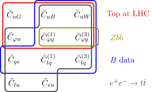
Figure 2: Schematic overview of dominant contributions from SMEFT coefficients to the different sets of observables considered in this work. Subleading contributions at one-loop level as well as mixing-induced ones from $\tilde{C}_{uG}$ are neglected.

IV Fits to present data

We employ EFTfitter Castro et al. (2016), which is based on the Bayesian Analysis Toolkit - BAT.jl Schulz et al. (2021), to constrain the Wilson coefficients in a Bayesian interpretation. We include systematic and statistical experimental and SM theory uncertainties. All uncertainties on the measured observables are assumed to be Gaussian distributed. The procedure of our fit is detailed in our previous analyses in Refs. Bißmann et al. (2020a, b), and is based on Ref. Castro et al. (2016).

BSM contributions are parametrized as in (19), which includes quadratic dimension-six terms. While these purely BSM contributions are formally of higher order in the EFT expansion, $\mathcal{O}(\Lambda^{-4})$, it has been shown Bißmann et al. (2020b); Hartland et al. (2019) that the inclusion of such quadratic terms has only a negligible effect on constraints of coefficients for which the linear term in the EFT expansion gives the dominant contribution, as expected in regions where the EFT is valid.

We include measurements of observables from both top-quark pair production processes and top-quark decay at the LHC, $Z\to b\bar{b}$ transitions, and $b\rightarrow s$ transitions from different experiments. Measurements of the same observable from different experiments can in principle be correlated Aaboud et al. (2019a). Correlations are included as long as they are provided, comprising mainly bin-to-bin correlations and correlations between the $W$ boson helicity fractions. Unknown correlations can affect the result of the fit significantly Bißmann et al. (2020b). Therefore, we follow a strategy similar to the ones of Refs. Durieux et al. (2019); Brivio et al. (2020) and include only the most precise measurement of an observable in the fit. Especially, if no complete correlation matrices for differential distributions are given by the experiments, we do not include these measurements in the analysis. For $B$ physics observables, a variety of measurements have been combined by the Heavy Flavour Averaging Group (HFLAV) Amhis et al. (2019). Wherever possible, we include their averaged experimental values in our analysis. For all remaining unknown correlations between different observables, we make the simplifying assumptions that the measurements included in the fit are uncorrelated.

We work out current constraints from top-quark measurements in Sec. IV.1, from $Z\to b\bar{b}$ data in Sec. IV.2, from $B$-physics in Sec. IV.3, and perform a global analysis in Sec. IV.4.

IV.1 Current constraints from top-quark measurements at the LHC

Process	Observable	$\sqrt{s}$	Int. luminosity	Experiment	Ref.	SM Ref.
$t\bar{t}\gamma$	$\sigma^{\mathrm{fid}}(t\bar{t}\gamma,1\ell)\,,\ \sigma^{\mathrm{fid}}(t\bar{t}\gamma,2\ell)$	13 TeV	36.1 $\textmd{fb}^{-1}$	ATLAS	Aaboud et al. (2019b)	Aaboud et al. (2019b); Melnikov et al. (2011)
$t\bar{t}Z$	$\sigma^{\mathrm{inc}}(t\bar{t}Z)$	13 TeV	77.5 $\textmd{fb}^{-1}$	CMS	Sirunyan et al. (2020a)	Frixione et al. (2015); de Florian et al. (2016); Frederix et al. (2018)
$t\bar{t}$	$\sigma^{\textmd{inc}}(t\bar{t})$	13 TeV	36.1 $\textmd{fb}^{-1}$	ATLAS	Aad et al. (2019)	Czakon and Mitov (2014)
	$F_{0}\,,\ F_{L}$	8 TeV	20.2 $\textmd{fb}^{-1}$	ATLAS	Aaboud et al. (2017)	Czarnecki et al. (2010)
	$\Gamma_{t}$	8 TeV	20.2 $\textmd{fb}^{-1}$	ATLAS	Aaboud et al. (2018)	Gao et al. (2013)

Table 2: Considered observables for top-quark processes at the LHC and references for the corresponding measurements and SM calculations.

In Tab. 2 we summarize the measurements and the corresponding SM predictions of the top-quark observables at the LHC included in the fit. This dataset comprises measurements of fiducal cross sections $\sigma^{\textmd{fid}}(t\bar{t}\gamma,1\ell)$ ($\sigma^{\textmd{fid}}(t\bar{t}\gamma,2\ell)$) of $t\bar{t}\gamma$ production in the single lepton (dilepton) channel, inclusive cross sections $\sigma^{\textmd{inc}}(t\bar{t})$ and $\sigma^{\textmd{inc}}(t\bar{t}Z)$ of $t\bar{t}$ and $t\bar{t}Z$ production, respectively, measurements of the $W$ boson helicity fractions $F_{0,L}$, and a measurement of the total top-quark decay width $\Gamma_{t}$. The SM predictions for $t\bar{t}\gamma$ cross sections include NLO QCD corrections Refs. Aaboud et al. (2019b); Melnikov et al. (2011), while predictions for $t\bar{t}Z$ cross sections are computed at NLO QCD including electroweak corrections Frixione et al. (2015); de Florian et al. (2016); Frederix et al. (2018). For $t\bar{t}$ production, the SM prediction at NNLO QCD is taken from Ref. Aad et al. (2019), and has been computed following Ref. Czakon and Mitov (2014). Predictions for helicity fractions and the total decay width include NNLO QCD corrections Czarnecki et al. (2010); Gao et al. (2013).

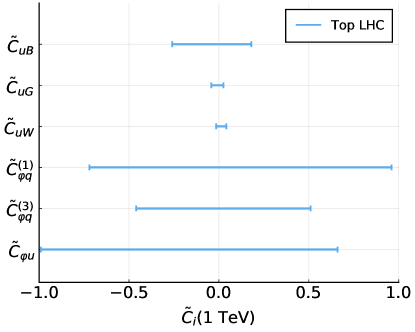
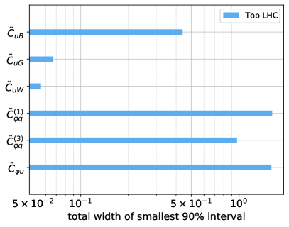
Figure 3: Constraints on SMEFT Wilson coefficients $\tilde{C}_{i}$ from the measurements of top-quark observables in Tab. 2. Shown are the marginalized smallest intervals containing $90\text{\,}\mathrm{\char 37\relax}$ posterior probability (left) and the total width of these intervals (right) obtained in a fit of six coefficients to top-quark data. For all coefficients we choose a uniform distribution in the interval $-1\leq\tilde{C}_{i}\leq 1$ as the prior probability.

In Fig. 3 we give constraints on SMEFT Wilson coefficients detailed in Tab. 1 obtained in a fit of six coefficients to the data in Tab. 2. The strongest constraints are found for $\tilde{C}_{uG}$ and $\tilde{C}_{uW}$, which are at the level of $\mathcal{O}(10^{-2})$ and stem from measurements of $t\bar{t}$ production cross sections and the $W$ boson helicity fractions, respectively. Constraints on $\tilde{C}_{uB}$, which are dominated by $t\bar{t}\gamma$ measurements, are at the level of $\mathcal{O}(10^{-1})$. Including measurements of the top-quark decay width allows constraining $\tilde{C}^{(3)}_{\varphi q}$ to a level of $\mathcal{O}(1)$. Given present data, results are limited by large experimental uncertainties. Both $\tilde{C}^{(1)}_{\varphi q}$ and $\tilde{C}_{\varphi u}$ remain almost unconstrained by the measurements of $t\bar{t}Z$ production due to a strong correlation between their contributions and larger uncertainties of measurements and theory predictions.

IV.2 Constraints from $Zbb$ measurements

Precision measurements of $Z$ pole observables have been performed at LEP 1 and SLC, and the results are collected in Ref. Zyla et al. (2020). In our analysis, we focus on those that are sensitive to BSM contributions which affect the $Zb\bar{b}$ vertex. The measurements included are those of the forward-backward asymmetry and the ratio of partial widths for $Z\rightarrow f\bar{f}$ Schael et al. (2006)

$$A^{0,b}_{FB}{}^{\textmd{Exp}}=0.0996\pm 0.0016\,,\quad R_{b}{}^{\textmd{Exp}}=0.21629\pm 0.00066\,.$$ (27)

The corresponding SM values are given as Schael et al. (2006); Zyla et al. (2020)

$$A^{0,b}_{FB}{}^{\textmd{SM}}=0.1030\pm 0.0002\,,\quad R_{b}^{\textmd{SM}}=0.21581\pm 0.00002\,.$$ (28)

These observables are sensitive to BSM contributions from $\tilde{C}^{+}_{\varphi q}$, which alter the $Zb\bar{b}$ vertex, and allow to derive strong constraints on this coefficient.

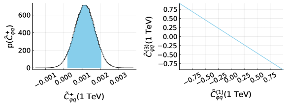
Figure 4: Results of fits to $Zb\bar{b}$ data considering $\tilde{C}^{+}_{\varphi q}$ (left) and $\tilde{C}^{(1)}_{\varphi q}$ and $\tilde{C}^{(3)}_{\varphi q}$ (right) as degrees of freedom. Shown are the one-dimensional (left) and two-dimensional (right) projection of the posterior distribution obtained in fits of one and two coefficients, respectively. Colored areas correspond to the smallest intervals containing 90 % of the posterior distribution. For the prior we consider an interval $-1\leq\tilde{C}_{i}\leq 1$.

The results of a fit of one ($\tilde{C}^{+}_{\varphi q}$) and two ($\tilde{C}^{(1)}_{\varphi q}$, $\tilde{C}^{(3)}_{\varphi q}$) coefficients to $Zb\bar{b}$ data are shown in Fig. 4. As can be seen, this dataset strongly constrains $\tilde{C}^{+}_{\varphi q}$ to a level of $\mathcal{O}(10^{-3})$. Due to the deviations from the SM present in $A^{0,b}_{FB}$ we observe deviations of about $2\,\sigma$ in $\tilde{C}^{+}_{\varphi q}$. Considering results in the $\tilde{C}^{(1)}_{\varphi q}$-$\tilde{C}^{(3)}_{\varphi q}$ plane we find, as expected, strong correlations, and only a very small slice of the two-dimensional parameter space is allowed by present data.

IV.3 Current constraints from $B$ physics measurements

Process	Observable	$q^{2}$ bin [GeV2]	Experiment	Ref.	SM Ref.
$\bar{B}\rightarrow X_{s}\gamma$	BR${}_{E_{\gamma}>1.6~{}\textmd{GeV}}$	-	HFLAV	Amhis et al. (2019)	Misiak et al. (2015)
$B^{0}\rightarrow K^{*}\gamma$	BR	-	HFLAV	Amhis et al. (2019)	Straub (2018)
$B^{+}\rightarrow K^{*+}\gamma$	BR	-	HFLAV	Amhis et al. (2019)	Straub (2018)
$\bar{B}\rightarrow X_{s}\ell^{+}\ell^{-}$	BR	${[1,6]}$	BaBar	Lees et al. (2014)	Huber et al. (2015)
	$A_{\textmd{FB}}$	${[1,6]}$	Belle	Sato et al. (2016)	Huber et al. (2015)
$B_{s}\rightarrow\mu^{+}\mu^{-}$	BR	-	LHCb	Archilli (2021)	Straub (2018)
${B}^{0}\rightarrow K^{*}\mu^{+}\mu^{-}$	$F_{L}\,,\ P_{1}\,,\ P_{2}\,,\ P_{3}\,,$ $\ P_{4}^{\prime}\,,\ P_{5}^{\prime}\,,\ P_{6}^{\prime}\,,\ P_{8}^{\prime}$	${[1.1,6]}$	LHCb	Aaij et al. (2020)	Straub (2018)
${B}^{0}\rightarrow K\mu^{+}\mu^{-}$	$d\text{BR}/dq^{2}$	${[1,6]}$	LHCb	Aaij et al. (2014)	Straub (2018)
${B}^{+}\rightarrow K^{+}\mu^{+}\mu^{-}$	$d\text{BR}/dq^{2}$	${[1,6]}$	LHCb	Aaij et al. (2014)	Straub (2018)
${B}^{+}\rightarrow K^{+*}\mu^{+}\mu^{-}$	$d\text{BR}/dq^{2}$	${[1,6]}$	LHCb	Aaij et al. (2014)	Straub (2018)
${B}_{s}\rightarrow\phi\mu^{+}\mu^{-}$	$F_{L}\,,\ S_{3}\,,\ S_{4}\,,\ S_{7}$	${[1,6]}$	LHCb	Aaij et al. (2015a)	Straub (2018)
${\Lambda}_{b}\rightarrow\Lambda\mu^{+}\mu^{-}$	$d\text{BR}/dq^{2}$	${[15,20]}$	LHCb	Aaij et al. (2015b)	Straub (2018)
$B_{s}-\bar{B}_{s}$ mixing	$\Delta M_{s}$	-	HFLAV	Amhis et al. (2019)	Di Luzio et al. (2019)

Table 3: $B$-physics measurements included in the fit. For observables measured in $q^{2}$ bins (where $q^{2}$ denotes the squared invariant dilepton mass) we include only one bin due to unknown correlations between different bins for consistency.

In Tab. 3 we give the $B$ physics observables and the corresponding references of the measurements and SM predictions considered in our fit. This dataset includes both inclusive and exclusive branching ratios of $b\rightarrow s\gamma$ transitions, total and differential branching ratios of various $b\rightarrow s\mu^{+}\mu^{-}$ processes, inclusive branching ratios and asymmetries of $b\rightarrow s\ell^{+}\ell^{-}$ transitions, and angular distributions of $B^{0}\to K^{*}\mu^{+}\mu^{-}$ and $B_{s}\to\phi\mu^{+}\mu^{-}$. In the case of $B_{s}\to\mu^{+}\mu^{-}$, we consider the latest results presented by the LHCb collaboration Archilli (2021). We compute SM predictions and uncertainties with flavio Straub (2018). In addition, we also include the mass difference $\Delta M_{s}$ measured in $B_{s}-\bar{B}_{s}$ mixing, with SM prediction from Ref. Di Luzio et al. (2019). Note that we do not take into account measurements of the $B\rightarrow K^{(*)}\nu\bar{\nu}$ branching ratios as only upper limits are presently available by Belle Lutz et al. (2013) and BaBar Lees et al. (2013), which can not be considered in EFTfitter.

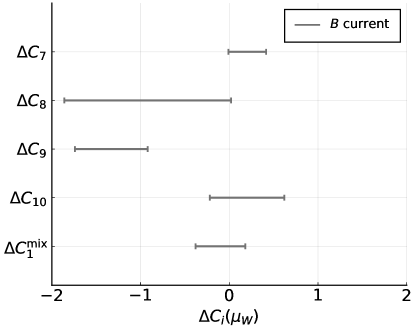
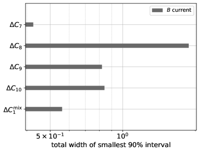
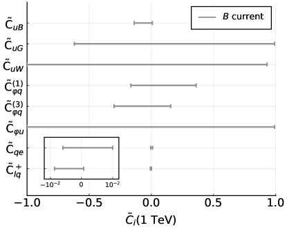
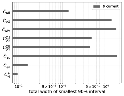
Figure 5: Constraints on WET coefficients $\Delta C_{i}$ at the scale $\mu=\mu_{W}$ (upper plots) and on SMEFT coefficients (lower plots) from measurements of $B$ observables in Tab. 3. Shown are the marginalized smallest intervals containing $90\text{\,}\mathrm{\char 37\relax}$ of the posterior probability (left) and the total width of these intervals (right) obtained in a fit of five WET (upper plots) and eight SMEFT coefficients (lower plots) to the data. The fit is performed using a uniform distribution over the interval $-2\leq\Delta C_{i}\leq 2$ ($-1\leq\tilde{C}_{i}\leq 1$) as a prior for the WET (SMEFT) coefficients.

In Fig. 5 (upper plots) we give constraints on BSM contributions $\Delta C_{i}$ to WET coefficients at the scale $\mu_{W}=m_{W}$ from a fit of five coefficients to the data in Tab. 3. The strongest constraints exist for $\Delta C^{\textmd{mix}}_{1}$ and $\Delta C_{7}$ for which the width of the smallest $90\text{\,}\mathrm{\char 37\relax}$ interval is about $5.5\times 10^{-1}$ and $4\times 10^{-1}$, respectively. The weakest constraints are obtained for $\Delta C_{8}$ as this coefficient contributes via mixing only. For $\Delta C_{9}$ we observe deviations from the SM. This effect stems mainly from measurements of angular distributions of $b\rightarrow s\mu^{+}\mu^{-}$ by LHCb and is widely known and discussed in literature, see e.g. Ref. Aebischer et al. (2019) for a detailed discussion. The exact deviation from the SM depends on the measurements considered in the fit. For the observables in Tab. 3 we find deviations mostly in $\Delta C_{9}$ while $\Delta C_{10}$ is SM like. The constraints on the WET coefficients $\Delta C_{i}$ can be translated into constraints on eight SMEFT coefficients (Fig. 5, lower plots) discussed in more detail in the next subsection, which are strongly correlated due to the matching conditions, see Eqs. (12)-(18). Nevertheless, strong constraints at the level of $\mathcal{O}(10^{-2})$ are found for the four-fermion coefficients. Constraints on the remaining coefficients are around one ($\tilde{C}_{uB}$, $\tilde{C}^{(1)}_{\varphi q}$, $\tilde{C}^{(3)}_{\varphi q}$) to two ($\tilde{C}_{uG}$, $\tilde{C}_{uW}$, $\tilde{C}_{\varphi u}$) orders of magnitude weaker. Note that deviations from the SM, which are present in the one-dimensional projection of the posterior distribution of $\Delta C_{9}$, can not be seen in the one-dimensional results in the SMEFT basis. This is due to the strong correlations among the SMEFT coefficients induced by the matching conditions.

IV.4 Combined fit to current data

Combining top-quark, $Zbb$, and $B$ observables allows to constrain a larger number of SMEFT coefficients compared to fits using only the individual datasets. Specifically, the coefficients constrained by data in Tabs. 2 and 3 and $Zbb$ data are

$$\tilde{C}_{uB}\,,\quad\tilde{C}_{uG}\,,\quad\tilde{C}_{uW}\,,\quad\tilde{C}_{\varphi q}^{(1)}\,,\quad\tilde{C}_{\varphi q}^{(3)}\,,\quad\tilde{C}_{\varphi u}\,,\quad\tilde{C}_{qe}\,,\quad\tilde{C}_{lq}^{+}\,.$$ (29)

From the fit of these eight coefficients to the combined dataset we obtain the results shown in Fig. 6.

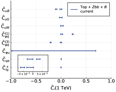
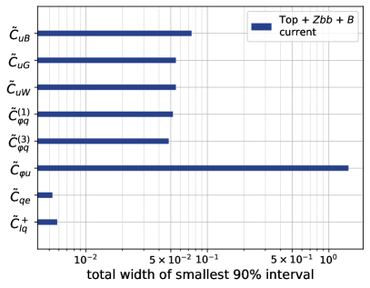
Figure 6: Constraints on SMEFT coefficients $\tilde{C}_{i}$ in Eq. (29) from a fit of eight coefficients to top-quark data in Tab. 2, $Zbb$ data, and $B$ physics data in Tab. 3. Shown are the smallest intervals containing $90\text{\,}\mathrm{\char 37\relax}$ posterior probability (left) and the total width of these intervals (right). For the prior we assume a uniform distribution over the interval $-1\leq\tilde{C}_{i}\leq 1$.

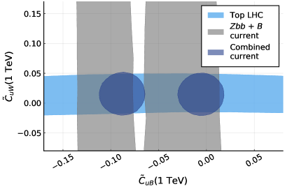
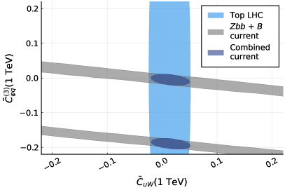
Figure 7: Examples for two-dimensional posterior distributions of SMEFT coefficients $\tilde{C}_{i}$ in Eq. (29) obtained in a fit of eight coefficients to top-quark data (light blue), $B$ physics data (grey) and the combined dataset including $Zbb$ data (blue). Shown are the smallest intervals containing $90\text{\,}\mathrm{\char 37\relax}$ of the posterior distribution. For the prior we assume a uniform distribution over the interval $-1\leq\tilde{C}_{i}\leq 1$.

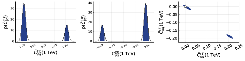
Figure 13: One-dimensional (left, middle) and two-dimensional (right) projections of the posterior distribution for $\tilde{C}^{(1)}_{\varphi q}$ and $\tilde{C}^{(3)}_{\varphi q}$. Results are obtained for a fit of eight SMEFT coefficients in Eq. (29) to the combined set of present top-quark, $Zb\bar{b}$, and $B$ physics data. The star in the rightmost plot denotes the SM point.

The strongest constraints are on $\tilde{C}_{qe}$ and $\tilde{C}^{+}_{lq}$, whose width of the smallest interval is around $(5-6)\times 10^{-3}$. This is expected, since both coefficients give sizable contributions to $\Delta C_{9}$ and $\Delta C_{10}$ at tree level (12). For $\tilde{C}_{uB}$, $\tilde{C}_{uG}$, $\tilde{C}_{uW}$, $\tilde{C}^{(1)}_{\varphi q}$ and $\tilde{C}^{(3)}_{\varphi q}$ the constraints are about one order of magnitude weaker, with a width of around $(5-7)\times 10^{-2}$. While constraints on $\tilde{C}_{uG}$ and $\tilde{C}_{uW}$ coincide with those derived from fits to top-quark data, the combination of the three datasets significantly tightens constraints on the other three coefficients. For $\tilde{C}_{uB}$ this enhancement stems from different sensitivities of top-quark and $B$ data, as already discovered in Ref. Bißmann et al. (2020a). The effect of the different datasets is shown in detail in Fig. 7 (left), where we give the two-dimensional projection of the posterior distributions obtained in fits to different datasets in the $\tilde{C}_{uB}$-$\tilde{C}_{uW}$ plane. Here, the effects are even more pronounced compared to Ref. Bißmann et al. (2020a), since a larger set of $B$ observables is considered here. Constraints on $\tilde{C}^{(1)}_{\varphi q}$ and $\tilde{C}^{(3)}_{\varphi q}$ (Fig. 6) are tightened by the inclusion of $Zbb$ data, which strongly constraints $\tilde{C}^{+}_{\varphi q}$, as well as the strong constraints on $\tilde{C}^{(3)}_{\varphi q}$, which arise from the combination of top-quark and $B$ physics data (see Fig. 7). As can be seen, in the combined fit the SM is included in the smallest intervals containing 90 % of the posterior distribution of $\tilde{C}^{(1)}_{\varphi q}$ and $\tilde{C}^{(3)}_{\varphi q}$, which is shown in detail in Fig. 13. The weakest constraints are found for $\tilde{C}_{\varphi u}$, since contributions to $B$ physics data are strongly suppressed, and $t\bar{t}Z$ production offers only a limited sensitivity, as we can already see in Fig. 3.

Interestingly, we find two solutions for several coefficients; one of which is SM like, while the other one deviates from the SM: $\tilde{C}_{uB}$, $\tilde{C}^{(1)}_{\varphi q}$, $\tilde{C}^{(3)}_{\varphi q}$, and the four-fermion coefficients $\tilde{C}_{qe}$ and $\tilde{C}^{+}_{lq}$. As can be seen in Fig. 7, the second solutions stem from the correlations between the coefficients introduced by matching the SMEFT basis onto the WET basis. Since the number of degrees of freedom is smaller in WET, correlations among the coefficients arise. Inclusion of top-quark data reduces these correlations, however, for the five coefficients the sensitivity of top-quark observables does not suffice to exclude the non-SM branches completely given present data and theory predictions. Without further input this ambiguity cannot be resolved.

We compare our results to those reported in a recent study on $b\rightarrow s\ell^{+}\ell^{-}$ transitions Ciuchini et al. (2020). In contrast to our analysis, operators are defined in a basis of diagonal down-type quark Yukawa couplings, which leads to an additional factor of $1/(V_{tb}V_{ts}^{*})$. Taking this factor into account, the results from Ciuchini et al. (2020) correspond to $\tilde{C}^{+}_{lq},\tilde{C}_{qe}\sim 10^{-3}$, consistent with Fig. 6. Repeating our fit with $\tilde{C}_{qe}$ and $\tilde{C}^{+}_{lq}$ only, we find agreement with Ref. Ciuchini et al. (2020).

We also comment on Drell-Yan production at the LHC. Amongst the couplings with top-quark focus considered in this works, (8), this concerns $\tilde{C}_{\varphi q}^{+}$, $\tilde{C}_{qe}$ and $\tilde{C}_{lq}^{+}$, just like $b\to s\ell^{+}\ell^{-}$ and $Z\to b\bar{b}$. Drell-Yan limits from existing data and a $3000\,\mbox{fb}^{-1}$ future projection for the semileptonic four-fermion operators with $b$-quarks are at the level of $\mathcal{O}(10^{-2})$ Greljo and Marzocca (2017); Fuentes-Martin et al. (2020), and weaker than in the combined fit, Fig. 6. Note, with the flavor of the initial quarks in $pp$-collisions undetermined an actual measurement of a quark flavor-specific coefficient is not possible. A detailed study of the implications of Drell-Yan processes for a global fit is beyond the scope of this work.

V Impact of future colliders

Both the HL-LHC operating at $14~{}$TeV with an integrated luminosity of $3000~{}$fb^-1 Atl (2019) and Belle II at $50~{}$ab^-1 Altmannshofer et al. (2019) are going to test the SM at the next level of precision. In Sec. V.1, we work out the impact of future measurements at these facilities on the SMEFT Wilson coefficients.

A first study of top-quark physics at the proposed lepton collider CLIC has been provided in Ref. Abramowicz et al. (2019). CLIC is intended to operate at three different center-of-mass energies: 380 GeV, 1.4 TeV, and 3 TeV and two different beam polarizations are foreseen by the accelerator design: a longitudinal polarization of $\pm 80\,\%$ for the electron beam and no polarization of the positron beam. We investigate the impact of measurements with the currently foreseen precision of such a lepton collider on the constraints of SMEFT Wilson coefficients in Sec. V.2.

We combine existing data with HL-LHC, Belle II and CLIC projections in Sec. V.3.

V.1 Expected constraints from HL-LHC and Belle II

For the expected experimental uncertainties at the HL-LHC and Belle II we adopt estimates of the expected precision by ATLAS, CMS and Belle II collaborations ATLAS (2018); Atl (2019); CMS (2018a, b); Altmannshofer et al. (2019). If no value for the systematic uncertainties is given, we assume that these uncertainties shrink by a factor of two compared to the current best measurement, which is the case for the $t\bar{t}$ and $t\bar{t}Z$ cross sections, the $W$ boson helicity fractions, and the top-quark decay width. In addition, we make the assumption that theory uncertainties shrink by a factor of two compared to the current SM uncertainties due to improved MC predictions and higher-order calculations. We summarize the observables and references for the expected experimental and theory precision at HL-LHC and Belle II in Tab. 4. For the purpose of the fit, we consider present central values of measurements for the future projections. If no measurement is available, we consider the SM for central values.

For fiducial cross sections of $t\bar{t}\gamma$ production, an analysis with the expected uncertainties is provided in Refs. ATLAS (2018); Atl (2019). For both the dilepton and single-lepton cross section we consider the precision of the channel with the largest experimental uncertainty as our estimate. For $t\bar{t}Z$ production we follow the analysis in Refs. CMS (2018a); Atl (2019) and scale statistical uncertainties according to the luminosity. For systematic uncertainties we assume for simplicity a reduction by a factor of 2. For estimating the expected precision of the total $t\bar{t}$ production cross section, we base our assumptions on the study of differential $t\bar{t}$ cross sections in Ref. CMS (2018b); Atl (2019). For the uncertainties we apply the same assumptions as for $t\bar{t}Z$. As the $W$ boson helicity fractions and the top-quark decay width are not discussed in Ref. Atl (2019), we treat them in the same way as the $t\bar{t}$ cross section for simplicity.

Process	Observable	$q^{2}$ bin [GeV2]	Experiment	Ref.	SM Ref.
$t\bar{t}\gamma$	$\sigma^{\mathrm{fid}}(t\bar{t}\gamma,1\ell)\,,\ \sigma^{\mathrm{fid}}(t\bar{t}\gamma,2\ell)$	-	ATLAS	ATLAS (2018); Atl (2019)	Aaboud et al. (2019b); Melnikov et al. (2011)
$t\bar{t}Z$	$\sigma^{\mathrm{inc}}(t\bar{t}Z)$	-	CMS	CMS (2018a); Atl (2019)	Frixione et al. (2015); de Florian et al. (2016); Frederix et al. (2018)
$t\bar{t}$	$\sigma^{\textmd{inc}}(t\bar{t})$	-	CMS	CMS (2018b); Atl (2019)	Czakon and Mitov (2014)
	$F_{0}\,,\ F_{L}$	-	-	-	Czarnecki et al. (2010)
	$\Gamma_{t}$	-	-	-	Gao et al. (2013)
$\bar{B}\rightarrow X_{s}\gamma$	BR${}_{E_{\gamma}>1.6~{}\textmd{GeV}}$	-	Belle II	Altmannshofer et al. (2019)	Misiak et al. (2015)
$B^{0}\rightarrow K^{*}\gamma$	BR	-	Belle II	Altmannshofer et al. (2019)	Straub (2018)
$B^{+}\rightarrow K^{+*}\gamma$	BR	-	Belle II	Altmannshofer et al. (2019)	Straub (2018)
$\bar{B}\rightarrow X_{s}\ell^{+}\ell^{-}$	BR, $A_{\textmd{FB}}$	${[3.5,6]}$	Belle II	Altmannshofer et al. (2019)	Huber et al. (2015)
${B}^{0}\rightarrow K^{*}\mu^{+}\mu^{-}$	$F_{L}$ , $P_{1}\,,\ P_{2}\,,\ P_{3}\,,$ $P_{4}^{\prime}\,,\ P_{5}^{\prime}\,,\ P_{6}^{\prime}\,,\ P_{8}^{\prime}$	${[1.1,2.5]}$, ${[2.5,4]}$, ${[4,6]}$	Belle II	Altmannshofer et al. (2019)	Straub (2018)
${B}^{0}\rightarrow K^{(*)}\nu\bar{\nu}$	BR	-	Belle II	Altmannshofer et al. (2019)	Straub (2018)

Table 4: Overview of observables considered at future HL-LHC and Belle II projections. For each process we denote the references for the experimental projection and the SM prediction. In case of the [1.1,2.5] $q^{2}$ bin for ${B}^{0}\rightarrow K^{*}\mu^{+}\mu^{-}$ we consider the Belle II projection of the [1.0,2.5] bin for the expected experimental uncertainties.

For measurements of $b\rightarrow s$ transitions we take the estimates in Ref. Altmannshofer et al. (2019) into account. For the $b\rightarrow s\gamma$ inclusive branching ratio we take the precision for the BR($\bar{B}\rightarrow X_{s}\gamma)_{E_{\gamma}>1.9~{}\textmd{GeV}}$ measurement and assume that the same uncertainties apply for $E_{\gamma}>1.6~{}\textmd{GeV}$. In case of $B^{(+)}\rightarrow K^{(+)*}\gamma$, we directly include the estimated precision in Ref. Altmannshofer et al. (2019). Similarly, for the inclusive decay $\bar{B}\rightarrow X_{s}\ell^{+}\ell^{-}$ we use the expected precision for the $3.5~{}\textmd{GeV}^{2}\leq q^{2}\leq 6~{}\textmd{GeV}^{2}$ bin. We also considered other bins for this observable and found very comparable sensitivity. Finally, for $B\rightarrow K^{*}\mu^{+}\mu^{-}$ we include the angular distribution observable $P^{(\prime)}_{i}$ in different $q^{2}$ bins, and study the implications of the anomalies found in present data of $b\rightarrow s\mu^{+}\mu^{-}$ angular distributions.

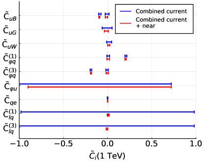
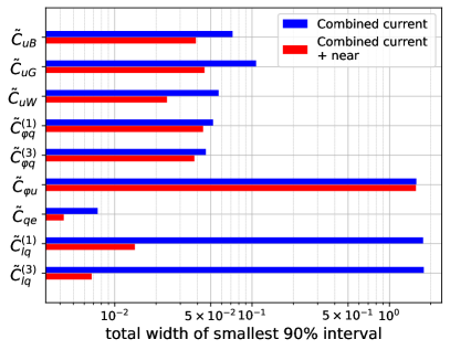
Figure 8: Constraints on coefficients $\tilde{C}_{i}$ from fits of nine coefficients to current top-quark and $B$ measurements in Tabs. 2 and 3 (blue) and to current measurments and projections of top-quark and $B$ observables in Tabs. 2-4 (red). Shown are the marginalized smallest intervals containing $90\text{\,}\mathrm{\char 37\relax}$ posterior probability (left) and the total widths of these intervals (right).

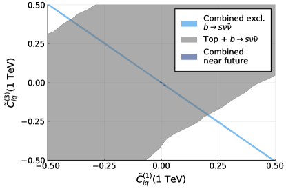
Figure 9: Two-dimensional projection of the posterior distribution in the $\tilde{C}^{(1)}_{lq}$-$\tilde{C}^{(3)}_{lq}$ plane. Shown are smallest intervals containing $90\text{\,}\mathrm{\char 37\relax}$ of the posterior distribution obtained in fits of nine coefficients in the near future projection combining top-quark observables with all beauty observables except $b\rightarrow s\nu\bar{\nu}$ ones (light blue), only with $b\rightarrow s\nu\bar{\nu}$ ones (grey), and the combined set (dark blue).

Combining top-quark and $B$ observables at HL-LHC and Belle II allows to test a total of nine SMEFT coefficients, see Fig. 8. In order to derive these constraints with EFTfitter, we have chosen a smaller prior $|\tilde{C}_{i}|\leq 0.1$ for the four-fermion coefficients because the posterior distribution lies only in a very small region, and a larger prior would lead to convergence issues. At this point, we neglect subleading contributions from $\tilde{C}_{eu}$ and $\tilde{C}_{lu}$, which are considered in Sec. V.3. As can be seen, the observables strongly constrain all coefficients except for $\tilde{C}_{\varphi u}$, which is only very weakly constrained, $\mathcal{O}(1)$, due to the low sensitivity in both $t\bar{t}Z$ and $B$ observables. Conversely, the strongest constraints are found for the four-fermion coefficients, around $4\times 10^{-3}$ and $(7-15)\times 10^{-3}$ for $\tilde{C}_{qe}$ and $\tilde{C}^{(1,3)}_{lq}$, respectively. The inclusion of $b\rightarrow s\nu\bar{\nu}$ observables allows to test $\tilde{C}^{(1)}_{lq}$ and $\tilde{C}^{(3)}_{lq}$ independently due to the orthogonal sensitivity compared to $b\rightarrow s\ell^{+}\ell^{-}$ observables, as indicated in Fig. 9. We observe that the interval obtained in the combined fit is significantly smaller than expected from the simple overlay of constraints from $b\rightarrow s\nu\bar{\nu}$ and $b\rightarrow s\ell^{+}\ell^{-}$ observables. The reason is, that the posterior distribution is constrained in the multi-dimensional hyperspace, and the combination significantly reduces correlations among different coefficients. In addition, we find that two solutions for $\tilde{C}^{(1)}_{lq}$ and $\tilde{C}^{(3)}_{lq}$ are allowed: one is close to the SM, while the other is around $\tilde{C}^{(1)}_{lq}\sim-\tilde{C}^{(3)}_{lq}\sim 10^{-3}$, and deviates strongly from the SM. Without further input, this ambiguity can not be resolved. Constraints on the remaining coefficients $\tilde{C}_{uB}$, $\tilde{C}_{uG}$, $\tilde{C}_{uW}$, $\tilde{C}^{(1)}_{\varphi q}$, and $\tilde{C}^{(3)}_{\varphi q}$ are in the range $(2-5)\times 10^{-2}$. Here, the higher precision in the near-future scenario tightens constraints on $\tilde{C}_{uB}$ ($t\bar{t}\gamma$ and $b\rightarrow s\gamma$), $\tilde{C}_{uG}$ ($t\bar{t}$), and $\tilde{C}_{uW}$ (helicity fractions) by a factor of around 2, while constraints on $\tilde{C}^{(1,3)}_{\varphi q}$ remain mostly unchanged. Note that the inclusion of additional measurements in the near-future projection does not suffice to resolve the second solutions observed for several coefficients.

V.2 CLIC projections

In Tab. 5 we list the top-quark observables for the CLIC future projections considered in this work. This set comprises total cross sections of $t\bar{t}$ production and forward-backward asymmetries $A_{\textmd{FB}}$ as observables for different energy stages and beam polarizations Abramowicz et al. (2019). We use the current SM predictions as nominal values, which include NLO QCD corrections Durieux et al. (2018b).

In Fig. 10 we give the results for a fit to the CLIC projections in Tab. 5. A smaller prior $|\tilde{C}_{i}|\leq 0.1$ is employed for the four-fermion coefficients due to the small size of the posterior distribution. We explicitly checked that we do not remove any solutions. Constraints on $\tilde{C}_{uG}$, which contributes via mixing only, are at the level of $4\times 10^{-1}$, and weaker compared to the ones on the remaining Wilson coefficients. For $\tilde{C}^{-}_{\varphi q}$ and $\tilde{C}_{\varphi u}$ the width of the smallest $90\text{\,}\mathrm{\char 37\relax}$ interval is at the level of $10^{-1}$. In comparison, constraints on $\tilde{C}_{uB}$ and $\tilde{C}_{uW}$ are found to be stronger by one order of magnitude. Even tighter constraints are obtained for four-fermion interactions, where the width of the smallest interval is at the level of $(2-6)\times 10^{-4}$.

Observable	$\sqrt{s}$	Polarization ($e^{-},e^{+}$)	Ref. experiment	SM Ref.
$\sigma_{t\bar{t}}$, $A_{\textmd{FB}}$	380 GeV	$(\pm$80\text{\,}\mathrm{\char 37\relax}$,0)$	Abramowicz et al. (2019)	Durieux et al. (2018b)
$\sigma_{t\bar{t}}$, $A_{\textmd{FB}}$	1.4 TeV	$(\pm$80\text{\,}\mathrm{\char 37\relax}$,0)$	Abramowicz et al. (2019)	Durieux et al. (2018b)
$\sigma_{t\bar{t}}$, $A_{\textmd{FB}}$	3 TeV	$(\pm$80\text{\,}\mathrm{\char 37\relax}$,0)$	Abramowicz et al. (2019)	Durieux et al. (2018b)

Table 5: Observables at different energies and polarizations for $t\bar{t}$ production at CLIC Abramowicz et al. (2019). SM predictions are taken from Durieux et al. (2018b).

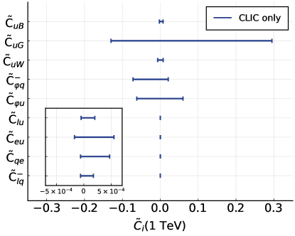
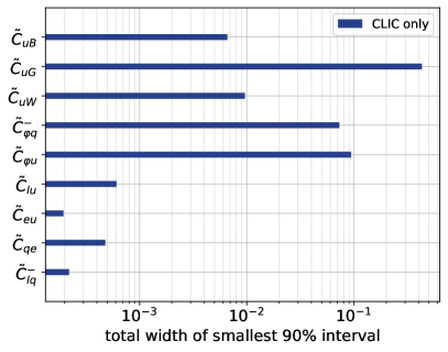
Figure 10: Constraints on coefficients $\tilde{C}_{i}$ from a fit of nine coefficients to CLIC observables in Tab. 5. Shown are the marginalized smallest intervals containing $90\text{\,}\mathrm{\char 37\relax}$ posterior probability (left) and the total widths of these intervals (right).

Interestingly, while Fig. 10 shows results of a fit treating $\tilde{C}^{-}_{lq}$ as a degree of freedom, the inclusion of RGE effects on $\tilde{C}^{(1)}_{lq}$ and $\tilde{C}^{(3)}_{lq}$ allows to distinguish both coefficients. The reason is that they develop differently under the RGE flow where corrections are at the level of $\mathcal{O}(1)\,\%$. Thus, both coefficients can be constrained simultaneously to a level of $\mathcal{O}(10^{-2})$, as shown in detail in Fig. 11.

V.3 Combined fit

Combining measurements and near-future projections of top-quark physics and $B$ physics in Tabs. 2-4 with the projections for top-quark observables at a CLIC-like lepton collider allows to constrain all eleven SMEFT coefficients considered in this analysis.

In Fig. 11 we give results from fits of all eleven coefficients to current data (Tabs. 2, 3, and $Zb\bar{b}$ data) and near-future projections (Tab. 4) (light blue), to CLIC projections for top-quark observables (Tab. 5) (grey) and the combined set (blue). It can be observed that the fit to the combined set of observables allows to constrain all eleven SMEFT Wilson coefficients. Flat directions in the parameter space of the coefficients are removed in the global fit. The strongest constraints are obtained for the four-fermion operators and are at the level of $\mathcal{O}(10^{-4})$. Constraints on the other operators are weaker and at the level of $\mathcal{O}(10^{-1})$ for $\tilde{C}_{\varphi u}$ and $\mathcal{O}(10^{-2})$ for the remaining coefficients.

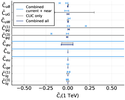
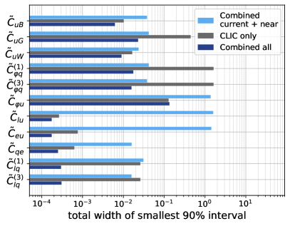
Figure 11: Constraints on coefficients $\tilde{C}_{i}$ obtained fitting eleven coefficients to top-quark and $B$ data and near-future projections at HL-LHC and Belle II in Tabs. 2-4 and CLIC future projections in Tab. 5. Shown are the marginalized smallest intervals containing $90\text{\,}\mathrm{\char 37\relax}$ posterior probability (left) and the total widths of these intervals (right).

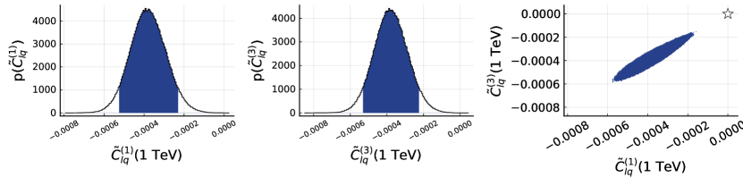
Figure 14: One-dimensional (left, middle) and two-dimensional (right) projections of the posterior distribution for $\tilde{C}^{(1)}_{lq}$ and $\tilde{C}^{(3)}_{lq}$. Results are obtained for a fit of all eleven coefficients in Eq. (8) to the combined set of present data, near future projections, and CLIC projections for top-quark observables. The star in the rightmost plot denotes the SM point.

As learned previously, combining different sets of observables yields stronger constraints on all coefficients. In the case of $\tilde{C}_{\varphi q}^{(1)}$ and $\tilde{C}_{\varphi q}^{(3)}$, which are already strongly constrained by present data and Belle II and HL-LHC projections, additional constrains derived from CLIC projections are orthogonal to those from the remaining observables, see Fig. 12 (left). This tightens the constraints by a factor of two and allows to exclude the second solution. Similarly, the second solution for $\tilde{C}_{uB}$ still present in the near-future scenario is removed as well. The improvement is particularly significant for $\tilde{C}^{(1)}_{lq}$ and $\tilde{C}^{(3)}_{lq}$. While $b\to s\ell^{+}\ell^{-}$ and $b\rightarrow s\nu\bar{\nu}$ observables allow to test both coefficients simultaneously, the inclusion of CLIC observables is mandatory to remove the second solution, see Fig. 12 (right). Correlations, which are induced by CLIC observables, between both coefficients are still present, and sizable deviations from the SM can be found, which is shown in more detail in Fig. 14 in App. F.

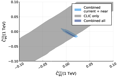
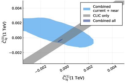
Figure 12: Examples for two-dimensional marginalized posterior distributions of SMEFT coefficients $\tilde{C}_{i}$ obtained in a fit of all eleven coefficients to top-quark and $B$ data in Tabs. 2-4 (light blue), top-quark observables at CLIC in Tab. 5 (grey) and the combined set (blue). Shown are the smallest regions containing $90\text{\,}\mathrm{\char 37\relax}$ posterior probability. Constraints from the fit on the combined set are so strong that the smallest $90\text{\,}\mathrm{\char 37\relax}$ region is barely visible in the $\tilde{C}^{(1)}_{lq}$-$C^{(3)}_{lq}$ plane (plot to the right).

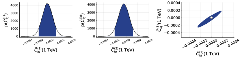
Figure 15: The same as in Fig. 14 but assuming SM central values for $b\to s$ observables at Belle II.

These deviations stem from the assumption that Belle II confirms present LHCb data. Interestingly, even though CLIC observables strongly constrain $\tilde{C}^{-}_{lq}$ (assuming that the SM value is measured), the exact position of the smallest 90 % interval on the $\tilde{C}^{(1)}_{\ell q}\sim-\tilde{C}^{(3)}_{\ell q}$ subspace is determined by Belle II results (Fig. 14). A scenario, in which we assume SM values for Belle II observables, is shown in Fig. 15 in App. F, and we find agreement with the SM in this case. While indeed constraints from CLIC projections and top-quark and $B$ data and projections in the near-future scenario have a different sensitivity, the $90\text{\,}\mathrm{\char 37\relax}$ region for $\tilde{C}^{(1)}_{lq}$ and $\tilde{C}^{(3)}_{lq}$ is significantly smaller than expected by simply overlaying the constraints obtained in fits to the two individual datasets. The reason is that constraints are combined in the full eleven-dimensional hyperspace, and Fig. 12 only shows two-dimensional projections.

As anticipated in Sec. II.2 the full, global fit results including CLIC projections are obtained assuming lepton-flavor universality. While in BSM scenarios where lepton generations couple differently the results cannot be applied directly, the findings on the orthogonality of the constraints and synergies between top and beauty continue to hold.

VI Conclusions

We performed fits within SMEFT to top-quark pair production, decay, $Z\to b\bar{b}$ transitions, and $b\rightarrow s$ transitions. We highlight how each of the individual datasets constrains different sets of Wilson coefficients of dimension-six operators affecting top-quark physics at present and future colliders. Extending previous works Bißmann et al. (2020a), we put an emphasis on semileptonic four-fermion operators, which are of high interest as they may be anomalous according to current flavor data and moreover are essentially unconstrained for top quarks. $SU(2)_{L}$ invariance leads to relations between up-type and down-type quark observables, a well-known feature with recent applications in semileptonic processes within SMEFT Bause et al. (2020). Here, we exploit this symmetry link between top and beauty observabes at the LHC and a future lepton collider.

Using existing data in Tabs. 2 and 3 as well as $Zbb$ data we constrain eight SMEFT Wilson coefficients with results shown in Fig. 6. Combining complementary constraints significantly improves the fits compared to using individual datasets alone, see Fig. 7. Going beyond existing data, we entertain a near-future scenario with measurements from Belle II and the HL-LHC, and one with an additional lepton collider. While measurements of top-quark observables at the HL-LHC allow to put stronger constraints on the same set of coefficients already tested by present top-quark measurements, a notable qualitative improvement in the near future is the expected observation of $b\to s\nu\bar{\nu}$ transitions at Belle II, which together with lepton universality allows to probe four-fermion operators in new ways: orthogonal to $b\to s\ell^{+}\ell^{-}$ and very similar as in contact interactions of leptons and top quarks, see Fig. 1. Thus, in this near-future scenario a combined fit would allow to probe nine SMEFT coefficients with estimated precision shown in Fig. 8. Combining the present data and projections for near-future experiments together with projections for a CLIC-like lepton collider, a combined fit enables to constrain the eleven SMEFT coefficients considered in this work, see Eq. (8), as shown in Fig. 11. The second solution for $\tilde{C}^{(1)}_{lq}$ and $\tilde{C}^{(3)}_{lq}$ present in fits in the near-future scenario, see Fig. 8, could be removed by lepton collider measurements, as demonstrated in Fig. 12. We stress that a lepton collider allows to probe the coefficients $\tilde{C}_{\varphi u}$, $\tilde{C}_{lu}$ $\tilde{C}_{eu}$, which would otherwise remain loosely constrained in the fit. In the combined fit, constraints on four-fermion coefficients are obtained at the level of $\mathcal{O}(10^{-4})$.

To conclude, in order to extract the strongest constraints on SMEFT coefficients from a global fit of the SMEFT top-quark sector and of relevance to the $b$-anomalies, different collider setups as well as $SU(2)_{L}$ relations have to be employed to remove flat directions and to test all possible sources of BSM contributions simultaneously. The present study clearly demonstrates the strong new physics impact of a future lepton collider.

Note added: During the finalization of this project a preprint appeared by CMS in which SMEFT coefficients are constrained by top production in association with leptons at the $\sqrt{s}=13$ TeV LHC with $41.5\,\mbox{fb}^{-1}$ Sirunyan et al. (2020b). The constraints on four-fermion coefficients $\tilde{C}_{qe}$ and $\tilde{C}^{-}_{lq}$ are more than one order of magnitude weaker compared to ours using current data, Fig. 6. However, the CMS-analysis is sensitive to $\tilde{C}_{eu}$, $\tilde{C}_{lu}$, otherwise unconstrained by present data. A study of the future physics potential of this type of analysis would be desirable, however, requires detector-level simulations and is beyond the scope of this work.

Appendix A Weak effective theory

At energies below the scale $\mu_{W}\sim m_{W}$, physical processes are described by the Weak Effective Theory (WET). All BSM particles which are heavier than $m_{W}$ as well as the top quark and the $W$, $Z$ and Higgs bosons are integrated out. Both $b\rightarrow s\ell^{+}\ell^{-}$ and $b\rightarrow s\gamma$ transitions are described by the following Lagrangian:

$$\mathcal{L}_{\text{WET}}^{bs}=\frac{4G_{F}}{\sqrt{2}}V_{ts}^{*}V_{tb}\sum_{i=1}^{10}C_{i}(\mu)Q_{i}(\mu)\,.$$ (30)

Here, $G_{F}$ is the Fermi-constant, $C_{i}$ are Wilson coefficients and $Q_{i}$ are the corresponding effective operators which are defined as follows:

$$\begin{aligned} Q_{1}&=(\bar{s}_{L}\gamma_{\mu}T^{a}c_{L})(\bar{c}_{L}\gamma^{\mu}T^{a}b_{L})\,,&Q_{2}&=(\bar{s}_{L}\gamma_{\mu}c_{L})(\bar{c}_{L}\gamma^{\mu}b_{L})\,,\\ Q_{3}&=(\bar{s}_{L}\gamma_{\mu}b_{L})\sum_{q}(\bar{q}\gamma^{\mu}q)\,,&Q_{4}&=(\bar{s}_{L}\gamma_{\mu}T^{a}b_{L})\sum_{q}(\bar{q}\gamma^{\mu}T^{a}q)\,,\\ Q_{5}&=(\bar{s}_{L}\gamma_{\mu}\gamma_{\nu}\gamma_{\sigma}b_{L})\sum_{q}(\bar{q}\gamma^{\mu}\gamma^{\nu}\gamma^{\sigma}q)\,,&Q_{6}&=(\bar{s}_{L}\gamma_{\mu}\gamma_{\nu}\gamma_{\sigma}T^{a}b_{L})\sum_{q}(\bar{q}\gamma^{\mu}\gamma^{\nu}\gamma^{\sigma}T^{a}q)\,,\\ Q_{7}&=\frac{e}{16\pi^{2}}m_{b}(\bar{s}_{L}\sigma^{\mu\nu}b_{R})F_{\mu\nu}\,,&Q_{8}&=\frac{g_{s}}{16\pi^{2}}m_{b}(\bar{s}_{L}\sigma^{\mu\nu}T^{a}b_{R})G^{a}_{\mu\nu}\,,\\ Q_{9}^{ij}&=\frac{e^{2}}{16\pi^{2}}(\bar{s}_{L}\gamma_{\mu}b_{L})(\bar{\ell}^{i}\gamma^{\mu}\ell^{j})\,,&Q_{10}^{ij}&=\frac{e^{2}}{16\pi^{2}}(\bar{s}_{L}\gamma_{\mu}b_{L})(\bar{\ell}^{i}\gamma^{\mu}\gamma_{5}\ell^{j})\,,\end{aligned}$$ (31)

with chiral left (right) projectors $L$ ($R$) and the field strength tensor of the photon $F_{\mu\nu}$. We denote charged leptons with $\ell$ and neglect contributions proportional to the subleading CKM-matrix element $V_{ub}$ and to the strange-quark mass.

The effective Lagrangian for $b\rightarrow s\bar{\nu}\nu$ transitions can be written as

$$\mathcal{L}_{\text{WET}}^{\nu}=\frac{4G_{F}}{\sqrt{2}}V_{ts}^{*}V_{tb}\sum_{i,j=1}^{3}\left(C_{L}^{ij}(\mu)Q_{L}^{ij}(\mu)+C_{R}^{ij}(\mu)Q_{R}^{ij}(\mu)\right)\,,$$ (32)

with effective operators

$$\begin{aligned} Q_{L}^{ij}=\frac{e^{2}}{16\pi^{2}}(\bar{s}_{L}\gamma_{\mu}b_{L})(\bar{\nu}^{i}\gamma^{\mu}(1-\gamma_{5})\nu^{j})\,,\quad Q_{R}^{ij}=\frac{e^{2}}{16\pi^{2}}(\bar{s}_{R}\gamma_{\mu}b_{R})(\bar{\nu}^{i}\gamma^{\mu}(1-\gamma_{5})\nu^{j})\,.\end{aligned}$$ (33)

Assuming flavor universality, only diagonal terms $i=j$ contribute, and all three flavors couple with identical strength. The $B_{s}-\bar{B}_{s}$ mass difference $\Delta M_{s}$ can be described as

$$\mathcal{L}_{\text{WET}}^{\textmd{mix}}=\frac{G_{F}^{2}m_{W}^{2}}{16\pi^{2}}Q_{1}^{\textmd{mix}}\left|V_{tb}V_{ts}^{*}\right|^{2}C_{1,tt}^{\textmd{mix}}\,,$$ (34)

with the effective operator

$$Q_{1}^{\textmd{mix}}=\left(\bar{s}_{L}\gamma_{\mu}b_{L}\right)\left(\bar{s}_{L}\gamma^{\mu}b_{L}\right)\,.$$ (35)

Appendix B SMEFT coefficients in the mass basis

In the up-mass basis we absorb the unitary rotations $S_{L,R}^{u}$ between the flavor and mass basis into the Wilson coefficients. The ones of the operators (2) are then given as

$$\begin{aligned} \hat{C}_{\varphi q}^{(1)ij}&=\hat{C}_{\varphi q}^{(1)kl}\left(S^{u\dagger}_{L}\right)_{ik}\left(S^{\vphantom{\dagger}u}_{L}\right)_{lj}\,,\enskip&\hat{C}_{\varphi q}^{(3)ij}&=\hat{C}_{\varphi q}^{(3)kl}\left(S^{u\dagger}_{L}\right)_{ik}\left(S^{\vphantom{\dagger}u}_{L}\right)_{lj}\,,\\ \hat{C}_{uB}^{ij}&=\hat{C}_{uB}^{kl}\left(S^{u\dagger}_{L}\right)_{ik}\left(S^{\vphantom{\dagger}u}_{R}\right)_{lj}\,,\enskip&\hat{C}_{uW}^{ij}&=\hat{C}_{uW}^{kl}\left(S^{u\dagger}_{L}\right)_{ik}\left(S^{\vphantom{\dagger}u}_{R}\right)_{lj}\,,\enskip\\ \hat{C}_{uG}^{ij}&=\hat{C}_{uG}^{kl}\left(S^{u\dagger}_{L}\right)_{ik}\left(S^{\vphantom{\dagger}u}_{R}\right)_{lj}\,,\enskip&\hat{C}_{\varphi u}^{ij}&=\hat{C}_{\varphi u}^{kl}\left(S^{u\dagger}_{R}\right)_{ik}\left(S^{\vphantom{\dagger}u}_{R}\right)_{lj}\,.\enskip\end{aligned}$$ (36)

Similarly, we obtain for the coefficients of the four-fermion operators (3)

$$\begin{aligned} \hat{C}^{(1)ij}_{lq}&=C^{(1)kl}_{lq}\left(S^{u\dagger}_{L}\right)_{ik}\left(S^{\vphantom{\dagger}u}_{L}\right)_{lj}\,,\enskip&\hat{C}^{(3)ij}_{lq}&=C^{(3)kl}_{lq}\left(S^{u\dagger}_{L}\right)_{ik}\left(S^{\vphantom{\dagger}u}_{L}\right)_{lj}\,,\\ \hat{C}^{ij}_{qe}&=C^{kl}_{qe}\left(S^{u\dagger}_{L}\right)_{ik}\left(S^{\vphantom{\dagger}u}_{L}\right)_{lj}\,,&\hat{C}^{ij}_{eu}&=C^{kl}_{eu}\left(S^{u\dagger}_{R}\right)_{ik}\left(S^{\vphantom{\dagger}u}_{R}\right)_{lj}\,,\enskip\\ \hat{C}^{ij}_{lu}&=C^{kl}_{lu}\left(S^{u\dagger}_{R}\right)_{ik}\left(S^{\vphantom{\dagger}u}_{R}\right)_{lj}\,.\end{aligned}$$ (37)

Appendix C SMEFT operators in the mass basis

In the up-mass eigenbasis, with coefficients defined according to Eq. (36) we find for the effective operators in Eq. (2)

$$\begin{aligned} \hat{C}_{\varphi q}^{(1)ij}\hat{O}_{\varphi q}^{(1)ij}=&\hat{C}_{\varphi q}^{(1)ij}\left(\varphi^{\dagger}i\overleftrightarrow{D}_{\mu}\varphi\right)\left(\bar{u}_{L}^{\prime i}\gamma^{\mu}u_{L}^{\prime j}+V^{\dagger}_{ki}V^{\vphantom{\dagger}}_{il}\bar{d}_{L}^{\prime k}\gamma^{\mu}d_{L}^{\prime l}\right)\,,\\ \hat{C}_{\varphi q}^{(3)ij}\hat{O}_{\varphi q}^{(3)ij}=&\hat{C}_{\varphi q}^{(3)ij}\left(\varphi^{\dagger}i\overleftrightarrow{D}_{\mu}^{3}\varphi\right)\left(\bar{u}_{L}^{\prime i}\gamma^{\mu}u_{L}^{\prime j}-V^{\dagger}_{ki}V^{\vphantom{\dagger}}_{jl}\bar{d}_{L}^{\prime k}\gamma^{\mu}d_{L}^{\prime l}\right)+\dots\,,\\ \hat{C}_{uB}^{ij}\hat{O}_{uB}^{ij}=&\hat{C}_{uB}^{ij}\left(\bar{u}^{\prime i}_{L}\sigma^{\mu\nu}u_{R}^{\prime j}\right)\frac{h+v}{\sqrt{2}}B_{\mu\nu}+\textmd{h.c.}\,,\\ \hat{C}_{uW}^{ij}\hat{O}_{uW}^{ij}=&\hat{C}_{uW}^{ij}\left[\left(\bar{u}^{\prime i}_{L}\sigma^{\mu\nu}u_{R}^{\prime j}\right)\frac{h+v}{\sqrt{2}}W^{3}_{\mu\nu}+V^{{\dagger}}_{ki}\left(\bar{d}^{\prime k}_{L}\sigma^{\mu\nu}u_{R}^{\prime j}\right)\frac{h+v}{\sqrt{2}}W^{-}_{\mu\nu}\right]+\textmd{h.c.}\,,\\ \hat{C}_{uG}^{ij}\hat{O}_{uG}^{ij}=&\hat{C}_{uG}^{ij}\left(\bar{u}^{\prime i}_{L}\sigma^{\mu\nu}T^{A}u_{R}^{\prime j}\right)\frac{h+v}{\sqrt{2}}G_{\mu\nu}^{A}+\textmd{h.c.}\,,\\ \hat{C}_{\varphi u}^{ij}\hat{O}_{\varphi u}^{ij}=&\hat{C}_{\varphi u}^{ij}\left(\varphi^{\dagger}i\overleftrightarrow{D}_{\mu}\varphi\right)\left(\bar{u}_{R}^{i}\gamma^{\mu}u_{R}^{j}\right)\,.\end{aligned}$$ (38)

Similarly, we find for the four-fermion operators in Eq. (3) with coefficients defined in Eq. (37)

$$\begin{aligned} \hat{C}_{lq}^{(1)ij}\hat{O}_{lq}^{(1)ij}=&\hat{C}_{lq}^{(1)ij}\left(\bar{l}_{L}\gamma_{\mu}l_{L}\right)\left(\bar{u}_{L}^{\prime i}\gamma^{\mu}u_{L}^{\prime j}+V^{\dagger}_{ki}V^{\vphantom{\dagger}}_{il}\bar{d}_{L}^{\prime k}\gamma^{\mu}d_{L}^{\prime l}\right)\,,\\ \hat{C}_{lq}^{(3)ij}\hat{O}_{lq}^{(3)ij}=&\hat{C}_{lq}^{(3)ij}\left(\bar{l}_{L}\gamma_{\mu}\tau^{3}l_{L}\right)\left(\bar{u}_{L}^{\prime i}\gamma^{\mu}u_{L}^{\prime j}-V^{\dagger}_{ki}V^{\vphantom{\dagger}}_{il}\bar{d}_{L}^{\prime k}\gamma^{\mu}d_{L}^{\prime l}\right)+\dots\,,\\ \hat{C}_{qe}^{(1)ij}\hat{O}_{qe}^{(1)ij}=&\hat{C}_{qe}^{(1)ij}\left(\bar{e}_{R}\gamma_{\mu}e_{R}\right)\left(\bar{u}_{L}^{\prime i}\gamma^{\mu}u_{L}^{\prime j}+V^{\dagger}_{ki}V^{\vphantom{\dagger}}_{il}\bar{d}_{L}^{\prime k}\gamma^{\mu}d_{L}^{\prime l}\right)\,,\\ \hat{C}_{eu}^{ij}\hat{O}_{eu}^{ij}=&\hat{C}_{eu}^{ij}\left(\bar{e}_{R}\gamma_{\mu}e_{R}\right)\left(\bar{u}_{R}^{\prime i}\gamma^{\mu}u_{R}^{\prime j}\right)\,,\\ \hat{C}_{lu}^{ij}\hat{O}_{lu}^{ij}=&\hat{C}_{lu}^{ij}\left(\bar{l}_{L}\gamma_{\mu}l_{L}\right)\left(\bar{u}_{R}^{\prime i}\gamma^{\mu}u_{R}^{\prime j}\right)\,.\end{aligned}$$ (39)

These results are in agreement with Ref. Aebischer et al. (2016).

Appendix D Analytic formulas for one-loop matching

The contributions from $\tilde{C}^{(i)}_{\varphi q}$ to $C_{7}$ and $C_{8}$ are taken from Dekens and Stoffer (2019):

$$E_{7}^{\varphi q}(x_{t}) =\frac{1}{27}(2\cos^{2}\theta_{w}+1)\,,$$ (40)

$$E_{7}^{\varphi q(3)}(x_{t}) =\frac{8x_{t}^{3}+5x_{t}^{2}-7x_{t}}{12(x_{t}-1)^{3}}+\frac{x_{t}^{2}(2-3x_{t})}{2(1-x_{t})^{4}}\log x_{t}+\frac{1}{54}(-4\cos^{2}\theta_{w}+67)\,,$$ (41)

$$E_{8}^{\varphi q}(x_{t}) =\frac{1}{9}(2\cos^{2}\theta_{w}+1)\,,$$ (42)

$$E_{8}^{\varphi q(3)}(x_{t}) =-\frac{x_{t}(x_{t}^{2}-5x_{t}-2)}{4(x_{t}-1)^{3}}-\frac{3}{2}\frac{x_{t}^{2}}{(x_{t}-1)^{4}}\log x_{t}+\frac{1}{9}(2\cos^{2}\theta_{w}+1)\,.$$ (43)

The remaining functions relevant for contributions from dipole operators read Aebischer et al. (2016)

$$\begin{aligned} E_{7}^{uW}(x_{t})&=\frac{-9x_{t}^{3}+63x_{t}^{2}-61x_{t}+19}{48\left(x_{t}-1\right)^{3}}+\frac{\left(3x_{t}^{4}-12x_{t}^{3}-9x_{t}^{2}+20x_{t}-8\right)\ln\left(x_{t}\right)}{24\left(x_{t}-1\right)^{4}}\\ &+\frac{1}{8}\ln\left(\frac{m_{W}^{2}}{\mu_{W}^{2}}\right)\,,\end{aligned}$$ (44)

$$F_{7}^{uW}(x_{t})=\frac{x_{t}\left(2-3x_{t}\right)\ln\left(x_{t}\right)}{4\left(x_{t}-1\right)^{4}}-\frac{3x_{t}^{3}-17x_{t}^{2}+4x_{t}+4}{24\left(x_{t}-1\right)^{3}}\,,$$ (45)

$$E_{7}^{uB}(x_{t})=-\frac{1}{8}\ln\left(\frac{m_{W}^{2}}{\mu_{W}^{2}}\right)-\frac{\left(x_{t}+1\right)^{2}}{16\left(x_{t}-1\right)^{2}}-\frac{x_{t}^{2}\left(x_{t}-3\right)\ln\left(x_{t}\right)}{8\left(x_{t}-1\right)^{3}}\,,$$ (46)

$$F_{7}^{uB}(x_{t})=-\frac{1}{8}\,,$$ (47)

$$E_{8}^{uW}(x_{t})=\frac{3x_{t}^{2}-13x_{t}+4}{8\left(x_{t}-1\right)^{3}}+\frac{\left(5x_{t}-2\right)\ln\left(x_{t}\right)}{4\left(x_{t}-1\right)^{4}}\,,$$ (48)

$$F_{8}^{uW}(x_{t})=\frac{x_{t}^{2}-5x_{t}-2}{8\left(x_{t}-1\right)^{3}}+\frac{3x_{t}\ln\left(x_{t}\right)}{4\left(x_{t}-1\right)^{4}}\,,$$ (49)

$$E_{8}^{uG}(x_{t})=E_{7}^{uB}(x_{t})\,,$$ (50)

$$F_{8}^{uG}(x_{t})=F_{7}^{uB}(x_{t})\,.$$ (51)

The following functions relevant for the matching of up-type dipole operators on $C_{9}$ and $C_{10}$ are taken from Ref. Aebischer et al. (2016) and read

$$Y_{uW}(x_{t}) =\frac{3x_{t}}{4(x_{t}-1)}-\frac{3x_{t}}{4(x_{t}-1)^{2}}\ln\left(x_{t}\right)\,,$$ (52)

$$Z_{uW}(x_{t}) =\frac{99x_{t}^{3}-136x_{t}^{2}-25x_{t}+50}{36(x_{t}-1)^{3}}-\frac{24x_{t}^{3}-45x_{t}^{2}+17x_{t}+2}{6(x_{t}-1)^{4}}\ln\left(x_{t}\right)\,,$$ (53)

$$Z_{uB}(x_{t}) =-\frac{x_{t}^{2}+3x_{t}-2}{4(x_{t}-1)^{2}}+\frac{3x_{t}-2}{2(x_{t}-1)^{3}}\ln\left(x_{t}\right)\,.$$ (54)

Contributions for both four-fermion operators and operators with two Higgs bosons can be parametrized in terms of functions Endo et al. (2020)

$$K_{0}(x,\mu) =-\frac{x}{32}\left[\ln\frac{\mu^{2}}{m_{W}^{2}}+\frac{3(x+1)}{2(x-1)}-\frac{x^{2}-2x+4}{(x-1)^{2}}\ln x\right]\,,$$ (55)

$$K_{1}(x,\mu) =\frac{x}{16}\left[\ln\frac{\mu^{2}}{m_{W}^{2}}+\frac{x-7}{2(x-1)}-\frac{x^{2}-2x-2}{(x-1)^{2}}\ln x\right]\,,$$ (56)

$$K_{2}(x,\mu) =-\frac{x}{8}\left[\ln\frac{\mu^{2}}{m_{W}^{2}}+1-\ln x\right]\,,$$ (57)

$$J_{2}(x) =\frac{x}{8}\,,$$ (58)

$$J_{3}(x,\mu) =-\frac{3}{16}x_{t}\left[\ln\frac{\mu^{2}}{m_{W}^{2}}+\frac{x_{t}+3}{2(x_{t}-1)}-\frac{x_{t}^{2}+1}{(x_{t}-1)^{2}}\ln x_{t}\right]\,,$$ (59)

$$B(x) =\frac{3}{16}x\left[\frac{1}{x-1}-\frac{1}{(x-1)^{2}}\ln x\right]\,,$$ (60)

$$D(x) =-\frac{2}{9}\ln x-\frac{x}{72}\left[\frac{82x^{2}-151x+63}{(x-1)^{3}}-\frac{10x^{3}+59x^{2}-138x+63}{(x-1)^{4}}\ln x\right]\,.$$ (61)

With these definitions, the functions appearing in the matching to $C_{9}$ and $C_{10}$ read Endo et al. (2020)

$$\begin{aligned} I_{1}(x_{t})&=-J_{2}(x_{t})-2K_{0}(x_{t},\mu_{W})\\ &=\frac{x_{t}}{16}\left[\ln\frac{\mu^{2}}{m_{W}^{2}}-\frac{x_{t}-7}{2(x_{t}-1)}-\frac{x_{t}^{2}-2x_{t}+4}{(x_{t}-1)^{2}}\ln x_{t}\right].\end{aligned}$$ (62)

$$\begin{aligned} I_{2}(x_{t})=&J_{2}(x_{t})+K_{2}(x_{t},\mu_{w})+K_{0}(x_{t},\mu)\\ =&-\frac{x_{t}}{32}\left(5\ln\frac{\mu_{W}^{2}}{m_{W}^{2}}+\frac{3(x_{t}+1)}{2(x_{t}-1)}-\frac{5x_{t}^{2}-10x_{t}+8}{(x_{t}-1)^{2}}\ln x_{t}\right)\,,\end{aligned}$$ (63)

$$\begin{aligned} I^{lq}(x_{t})=&-J_{2}(x_{t})+K_{2}(x_{t},\mu_{w})+K_{0}(x_{t},\mu)\\ =&-\frac{x_{t}}{32}\left(8+5\ln\frac{\mu_{W}^{2}}{m_{W}^{2}}+\frac{3(x_{t}+1)}{2(x_{t}-1)}-\frac{5x_{t}^{2}-10x_{t}+8}{(x_{t}-1)^{2}}\ln x_{t}\right)\,,\end{aligned}$$ (64)

$$\begin{aligned} I_{1}^{\varphi q}(x_{t})=&(-1+4\sin^{2}\theta_{w})\left(J_{2}(x_{t})+2J_{3}(x_{t})-K_{1}(x_{t})-3K_{0}(x_{t},\mu)\right)\\ &+2\left(B(x_{t})+2\sin^{2}\theta_{w}D(x_{t})\right)\\ =&(-1+4\sin^{2}\theta_{w})\frac{x_{t}}{32}\left(4-11\ln\frac{\mu_{W}^{2}}{m_{W}^{2}}-\frac{5x_{t}+13}{2(x_{t}-1)}+\frac{11x_{t}^{2}+2x_{t}-4}{(x_{t}-1)^{2}}\ln x_{t}\right)\\ &+\frac{3}{8}x\left[\frac{1}{x_{t}-1}-\frac{1}{(x_{t}-1)^{2}}\ln x_{t}\right]+\sin^{2}\theta_{w}\left\{-\frac{8}{9}\ln x_{t}\right.\\ &-\left.\frac{x_{t}}{18}\left[\frac{82x_{t}^{2}-151x_{t}+63}{(x_{t}-1)^{3}}-\frac{10x_{t}^{3}+59x_{t}^{2}-138x_{t}+63}{(x_{t}-1)^{4}}\ln x_{t}\right]\right\}\,,\end{aligned}$$ (65)

$$\begin{aligned} I_{2}^{\varphi q}(x_{t})=&\left(J_{2}(x_{t})+2J_{3}(x_{t})-K_{1}(x_{t})-3K_{0}(x_{t},\mu)\right)+2B(x_{t})\\ =&\frac{x_{t}}{32}\left(4-11\ln\frac{\mu_{W}^{2}}{m_{W}^{2}}-\frac{5x_{t}+37}{2(x_{t}-1)}+\frac{11x_{t}^{2}+2x_{t}+8}{(x_{t}-1)^{2}}\ln x_{t}\right)\,,\end{aligned}$$ (66)

where we neglected CKM-suppressed contributions $\sim|V_{ts}|^{2},\sim|V_{td}|^{2}$, which are smaller by a factor of at least $\sim 10^{-3}$.

The functions $H_{i}$ relevant for the matching of $\tilde{C}^{(1)}_{\varphi q}$ and $\tilde{C}^{(3)}_{\varphi q}$ onto $C_{1}^{\textmd{mix}}$ read Bobeth et al. (2017)

$$H_{1}(x_{t}) =-\frac{x_{t}-7}{4(x_{t}-1)}-\frac{x_{t}^{2}-2x_{t}+4}{2(x_{t}-1)^{2}}\ln x_{t}\,,$$ (67)

$$H_{1}(x_{t}) =+\frac{7x_{t}-25}{4(x_{t}-1)}-\frac{x_{t}^{2}-14x_{t}+4}{2(x_{t}-1)^{2}}\ln x_{t}\,.$$ (68)

Finally, functions relevant for the matching of SMEFT coefficients onto $C_{L}$ at one-loop level are taken from Dekens and Stoffer (2019). Here, we give results with all evanescent coefficients set to 1:

$$\begin{aligned} I^{\nu}_{uW}&=\frac{m_{t}}{m_{W}\sin^{2}\theta_{w}}\left(-\frac{3(x_{t}-2)}{4\sqrt{2}(x_{t}-1)}-\frac{3x_{t}\ln x_{t}}{\sqrt{2}(x_{t}-1)^{2}}\right)\,,\end{aligned}$$ (69)

$$\begin{aligned} I^{\nu(1)}_{\varphi q}&=\frac{1}{\sin^{2}\theta_{w}}\left(\frac{x_{t}}{8}-\frac{3x_{t}(x_{t}+1)}{32(x_{t}-1)}-\frac{x_{t}(x_{t}^{2}-2x_{t}+4)\ln\frac{\mu_{W}^{2}}{m_{t}^{2}}}{16(x_{t}-1)^{2}}+\frac{3x_{t}\ln\frac{\mu_{W}^{2}}{m_{W}^{2}}}{16\left(x_{t}-1\right)^{2}}\right.\\ &+\left.\frac{(2m_{W}^{2}+m_{Z}^{2})}{8m_{W}^{2}}-\frac{3x_{t}\ln\frac{\mu_{W}^{2}}{m_{t}^{2}}}{8}\right)\,,\end{aligned}$$ (70)

$$\begin{aligned} I^{\nu(3)}_{\varphi q}&=\frac{1}{\sin^{2}\theta_{w}}\left(-\frac{x_{t}}{8}+\frac{5x_{t}(x_{t}-7)}{32(x_{t}-1)}+\frac{x_{t}(7x_{t}^{2}-2x_{t}-20)\ln\frac{\mu_{W}^{2}}{m_{t}^{2}}}{16(x_{t}-1)^{2}}-\frac{3x_{t}(4x_{t}-9)\ln\frac{\mu_{W}^{2}}{m_{W}^{2}}}{16\left(x_{t}-1\right)^{2}}\right.\\ &+\left.\frac{19m_{W}^{2}+m_{Z}^{2}}{8m_{W}^{2}}-\frac{3\ln\frac{mu_{W}^{2}}{m_{W}^{2}}}{8}+\frac{3m_{W}^{2}\ln\frac{\mu_{W}^{2}}{m_{W}^{2}}}{4m_{W}}\right)\,,\end{aligned}$$ (71)

$$\begin{aligned} I^{\nu}_{lu}&=\frac{1}{\sin^{2}\theta_{w}}\left(-\frac{x_{t}(x_{t}-7)}{32(x_{t}-1)}+\frac{(x_{t}^{3}-2x_{t}^{2}+4x_{t})\ln\frac{\mu_{w}^{2}}{m_{t}^{2}}}{16(x_{t}-1)^{2}}-\frac{3x_{t}\ln\frac{\mu_{w}^{2}}{m_{W}^{2}}}{16(x_{t}-1)^{2}}\right)\,,\end{aligned}$$ (72)

$$\begin{aligned} I^{\nu(1)}_{lq}&=\frac{1}{\sin^{2}\theta_{w}}\left(\frac{x_{t}}{8}-\frac{3x_{t}(x_{t}+1)}{32(x_{t}-1)}-\frac{x_{t}(x_{t}^{2}-2x_{t}+4)\ln\frac{\mu_{W}^{2}}{m_{t}^{2}}}{16(x_{t}-1)^{2}}+\frac{3x_{t}\ln\frac{\mu_{W}^{2}}{m_{W}^{2}}}{16\left(x_{t}-1\right)^{2}}\right.\\ &+\left.\frac{11(2m_{W}^{2}+m_{Z}^{2})}{48m_{W}^{2}}+\frac{(2m_{W}^{2}+m_{Z}^{2})\ln\frac{\mu_{W}^{2}}{m_{Z}^{2}}}{8m_{W}}\right)\,,\end{aligned}$$ (73)

$$\begin{aligned} I^{\nu(3)}_{lq}&=\frac{1}{\sin^{2}\theta_{w}}\left(\frac{x_{t}}{8}-\frac{3x_{t}(x_{t}+1)}{32(x_{t}-1)}-\frac{x_{t}(x_{t}^{2}-26x_{t}+28)\ln\frac{\mu_{W}^{2}}{m_{t}^{2}}}{16(x_{t}-1)^{2}}+\frac{3x_{t}(8x_{t}-9)\ln\frac{\mu_{W}^{2}}{m_{W}^{2}}}{16\left(x_{t}-1\right)^{2}}\right.\\ &+\left.\frac{-154m_{W}^{2}-11m_{Z}^{2}}{48m_{W}^{2}}-\frac{3\ln\frac{mu_{W}^{2}}{m_{W}^{2}}}{2}-\frac{(2m_{W}^{2}+m_{Z}^{2})\ln\frac{\mu_{W}^{2}}{m_{Z}^{2}}}{8m_{W}}\right)\,.\end{aligned}$$ (74)

Appendix E Numerical matching conditions

The numerical values of the tree-level matching conditions in Eq. (12) read at $\mu_{W}=m_{W}$

$$\begin{aligned} \Delta C_{9}^{\textmd{tree}}&=402.1\left[\tilde{C}^{1}_{lq}+\tilde{C}^{3}_{lq}+\tilde{C}_{qe}\right]-44.53\left(\tilde{C}^{1}_{\varphi q}+\tilde{C}^{3}_{\varphi q}\right)\,,\\ \Delta C_{10}^{\textmd{tree}}&=402.1\left[-\tilde{C}^{1}_{lq}-\tilde{C}^{3}_{lq}+\tilde{C}_{qe}+\tilde{C}^{1}_{\varphi q}+\tilde{C}^{3}_{\varphi q}\right]\,,\\ \Delta C_{L}^{\textmd{tree}}&=402.1\left[\tilde{C}^{1}_{lq}-\tilde{C}^{3}_{lq}+\tilde{C}^{1}_{\varphi q}+\tilde{C}^{3}_{\varphi q}\right]\,.\end{aligned}$$ (75)

For the one-loop contributions in Eqs. (13)-(18) we obtain at $\mu_{W}=m_{W}$

$$\begin{aligned} \Delta C_{7}^{\textmd{loop}}=&-2.31\tilde{C}_{uB}+0.0925\tilde{C}_{uW}--0.132\tilde{C}_{\varphi q}^{(1)}+1.12\tilde{C}_{\varphi q}^{(3)}\,,\end{aligned}$$ (76)

$$\begin{aligned} \Delta C_{8}^{\textmd{loop}}=&-0.669\tilde{C}_{uG}+0.271\tilde{C}_{uW}+0.392\tilde{C}^{(1)}_{\varphi q}+1.05\tilde{C}^{(3)}_{\varphi q}\,,\end{aligned}$$ (77)

$$\begin{aligned} \Delta C_{9}^{\textmd{loop}}=&2.170\tilde{C}_{uW}+2.512\tilde{C}_{uB}-1.81\tilde{C}_{\varphi q}^{(1)}-1.96\tilde{C}_{\varphi q}^{(3)}+0.148\tilde{C}_{\varphi u}\\ &-1.898\left(\tilde{C}_{eu}+\tilde{C}_{lu}\right)-2.242\left(\tilde{C}^{(1)}_{lq}-\tilde{C}_{qe}\right)-4.444\tilde{C}^{(3)}_{lq}\,,\end{aligned}$$ (78)

$$\begin{aligned} \Delta C_{10}^{\textmd{loop}}=&-7.54\tilde{C}_{uW}+12.8\tilde{C}_{\varphi q}^{(1)}-3.43\tilde{C}_{\varphi q}^{(3)}-1.90\tilde{C}_{\varphi u}-1.90\left(\tilde{C}_{eu}-\tilde{C}_{lu}\right)\\ &-2.242\left(\tilde{C}^{(1)}_{lq}-\tilde{C}_{qe}\right)+4.444\tilde{C}^{(3)}_{lq}\,,\end{aligned}$$ (79)

$$\begin{aligned} \Delta C_{L}^{\textmd{loop}}=&-2.88\tilde{C}_{uW}+14.9\tilde{C}_{\varphi q}^{(1)}+0.332\tilde{C}_{\varphi q}^{(3)}-1.90\left(\tilde{C}_{\varphi u}+\tilde{C}_{lu}\right)\\ &+4.622\tilde{C}^{(1)}_{lq}+1.033\tilde{C}^{(3)}_{lq}\,,\end{aligned}$$ (80)

$$\begin{aligned} \Delta C_{1,tt}^{\textmd{mix, loop}}=&4.12\tilde{C}_{uW}+14.8\tilde{C}_{\varphi q}^{(1)}+11.6\tilde{C}_{\varphi q}^{(3)}\,.\end{aligned}$$ (81)

Appendix F Auxiliary Plots

References

- Degrande et al. (2018) C. Degrande, F. Maltoni, K. Mimasu, E. Vryonidou, and C. Zhang, JHEP 10, 005 (2018), eprint 1804.07773.
- Chala et al. (2019) M. Chala, J. Santiago, and M. Spannowsky, JHEP 04, 014 (2019), eprint 1809.09624.
- Durieux et al. (2015) G. Durieux, F. Maltoni, and C. Zhang, Phys. Rev. D 91, 074017 (2015), eprint 1412.7166.
- Aguilar-Saavedra (2011) J. Aguilar-Saavedra, Nucl. Phys. B 843, 638 (2011), [Erratum: Nucl.Phys.B 851, 443–444 (2011)], eprint 1008.3562.
- D’Hondt et al. (2018) J. D’Hondt, A. Mariotti, K. Mimasu, S. Moortgat, and C. Zhang, JHEP 11, 131 (2018), eprint 1807.02130.
- Durieux et al. (2018a) G. Durieux, J. Gu, E. Vryonidou, and C. Zhang, Chin. Phys. C 42, 123107 (2018a), eprint 1809.03520.
- Buckley et al. (2015) A. Buckley, C. Englert, J. Ferrando, D. J. Miller, L. Moore, M. Russell, and C. D. White, Phys. Rev. D 92, 091501 (2015), eprint 1506.08845.
- Buckley et al. (2016) A. Buckley, C. Englert, J. Ferrando, D. J. Miller, L. Moore, M. Russell, and C. D. White, JHEP 04, 015 (2016), eprint 1512.03360.
- de Beurs et al. (2018) M. de Beurs, E. Laenen, M. Vreeswijk, and E. Vryonidou, Eur. Phys. J. C 78, 919 (2018), eprint 1807.03576.
- Brown et al. (2019) S. Brown, A. Buckley, C. Englert, J. Ferrando, P. Galler, D. J. Miller, L. Moore, M. Russell, C. White, and N. Warrack, PoS ICHEP2018, 293 (2019), eprint 1901.03164.
- Barducci et al. (2018) D. Barducci et al. (2018), eprint 1802.07237.
- Hartland et al. (2019) N. P. Hartland, F. Maltoni, E. R. Nocera, J. Rojo, E. Slade, E. Vryonidou, and C. Zhang, JHEP 04, 100 (2019), eprint 1901.05965.
- Maltoni et al. (2019) F. Maltoni, L. Mantani, and K. Mimasu, JHEP 10, 004 (2019), eprint 1904.05637.
- Durieux et al. (2019) G. Durieux, A. Irles, V. Miralles, A. Peñuelas, R. Pöschl, M. Perelló, and M. Vos, JHEP 12, 098 (2019), eprint 1907.10619.
- Neumann and Sullivan (2019) T. Neumann and Z. E. Sullivan, JHEP 06, 022 (2019), eprint 1903.11023.
- Brivio et al. (2020) I. Brivio, S. Bruggisser, F. Maltoni, R. Moutafis, T. Plehn, E. Vryonidou, S. Westhoff, and C. Zhang, JHEP 02, 131 (2020), eprint 1910.03606.
- Dror et al. (2016) J. A. Dror, M. Farina, E. Salvioni, and J. Serra, JHEP 01, 071 (2016), eprint 1511.03674.
- Bißmann et al. (2020a) S. Bißmann, J. Erdmann, C. Grunwald, G. Hiller, and K. Kröninger, Eur. Phys. J. C 80, 136 (2020a), eprint 1909.13632.
- Aoude et al. (2020) R. Aoude, T. Hurth, S. Renner, and W. Shepherd (2020), eprint 2003.05432.
- Fox et al. (2008) P. J. Fox, Z. Ligeti, M. Papucci, G. Perez, and M. D. Schwartz, Phys. Rev. D 78, 054008 (2008), eprint 0704.1482.
- Grzadkowski and Misiak (2008) B. Grzadkowski and M. Misiak, Phys. Rev. D 78, 077501 (2008), [Erratum: Phys.Rev.D 84, 059903 (2011)], eprint 0802.1413.
- Drobnak et al. (2012) J. Drobnak, S. Fajfer, and J. F. Kamenik, Nucl. Phys. B 855, 82 (2012), eprint 1109.2357.
- Brod et al. (2015) J. Brod, A. Greljo, E. Stamou, and P. Uttayarat, JHEP 02, 141 (2015), eprint 1408.0792.
- Bifani et al. (2019) S. Bifani, S. Descotes-Genon, A. Romero Vidal, and M.-H. Schune, J. Phys. G 46, 023001 (2019), eprint 1809.06229.
- Amjad et al. (2015) M. Amjad et al., Eur. Phys. J. C 75, 512 (2015), eprint 1505.06020.
- Amjad et al. (2013) M. Amjad, M. Boronat, T. Frisson, I. Garcia, R. Poschl, E. Ros, F. Richard, J. Rouene, P. Femenia, and M. Vos (2013), eprint 1307.8102.
- Abramowicz et al. (2019) H. Abramowicz et al. (CLICdp), JHEP 11, 003 (2019), eprint 1807.02441.
- Abada et al. (2019) A. Abada et al. (FCC), Eur. Phys. J. ST 228, 261 (2019).
- Kane et al. (1992) G. L. Kane, G. Ladinsky, and C. Yuan, Phys. Rev. D 45, 124 (1992).
- Atwood and Soni (1992) D. Atwood and A. Soni, Phys. Rev. D 45, 2405 (1992).
- Grzadkowski et al. (1997) B. Grzadkowski, Z. Hioki, and M. Szafranski, pp. 1113–1135 (1997), eprint hep-ph/9712357.
- Brzezinski et al. (1999) L. Brzezinski, B. Grzadkowski, and Z. Hioki, Int. J. Mod. Phys. A 14, 1261 (1999), eprint hep-ph/9710358.
- Boos et al. (2000) E. Boos, M. Dubinin, M. Sachwitz, and H. Schreiber, Eur. Phys. J. C 16, 269 (2000), eprint hep-ph/0001048.
- Jezabek et al. (2000) M. Jezabek, T. Nagano, and Y. Sumino, Phys. Rev. D 62, 014034 (2000), eprint hep-ph/0001322.
- Grzadkowski and Hioki (2000) B. Grzadkowski and Z. Hioki, Nucl. Phys. B 585, 3 (2000), [Erratum: Nucl.Phys.B 894, 585–587 (2015)], eprint hep-ph/0004223.
- Janot (2015) P. Janot, JHEP 04, 182 (2015), eprint 1503.01325.
- Röntsch and Schulze (2015) R. Röntsch and M. Schulze, JHEP 08, 044 (2015), eprint 1501.05939.
- Khiem et al. (2015) P. Khiem, E. Kou, Y. Kurihara, and F. Le Diberder (2015), eprint 1503.04247.
- Englert and Russell (2017) C. Englert and M. Russell, Eur. Phys. J. C 77, 535 (2017), eprint 1704.01782.
- Durieux et al. (2018b) G. Durieux, M. Perelló, M. Vos, and C. Zhang, JHEP 10, 168 (2018b), eprint 1807.02121.
- Cao and Yan (2015) Q.-H. Cao and B. Yan, Phys. Rev. D 92, 094018 (2015), eprint 1507.06204.
- Atl (2019) CERN Yellow Rep. Monogr. 7, Addendum (2019), eprint 1902.10229.
- Altmannshofer et al. (2019) W. Altmannshofer et al. (Belle-II), PTEP 2019, 123C01 (2019), [Erratum: PTEP 2020, 029201 (2020)], eprint 1808.10567.
- Weinberg (1979) S. Weinberg, Physica A 96, 327 (1979).
- Buchmuller and Wyler (1986) W. Buchmuller and D. Wyler, Nucl. Phys. B 268, 621 (1986).
- Degrande et al. (2013) C. Degrande, N. Greiner, W. Kilian, O. Mattelaer, H. Mebane, T. Stelzer, S. Willenbrock, and C. Zhang, Annals Phys. 335, 21 (2013), eprint 1205.4231.
- Kobach (2016) A. Kobach, Phys. Lett. B 758, 455 (2016), eprint 1604.05726.
- Grzadkowski et al. (2010) B. Grzadkowski, M. Iskrzynski, M. Misiak, and J. Rosiek, JHEP 10, 085 (2010), eprint 1008.4884.
- Bißmann et al. (2020b) S. Bißmann, J. Erdmann, C. Grunwald, G. Hiller, and K. Kröninger, Phys. Rev. D 102, 115019 (2020b), eprint 1912.06090.
- Zyla et al. (2020) P. Zyla et al. (Particle Data Group), PTEP 2020, 083C01 (2020).
- Aebischer et al. (2016) J. Aebischer, A. Crivellin, M. Fael, and C. Greub, JHEP 05, 037 (2016), eprint 1512.02830.
- Bause et al. (2020) R. Bause, H. Gisbert, M. Golz, and G. Hiller (2020), eprint 2007.05001.
- Hiller (2014) G. Hiller, APS Physics 7, 102 (2014).
- Jenkins et al. (2013a) E. E. Jenkins, A. V. Manohar, and M. Trott, Phys. Lett. B 726, 697 (2013a), eprint 1309.0819.
- Jenkins et al. (2013b) E. E. Jenkins, A. V. Manohar, and M. Trott, JHEP 10, 087 (2013b), eprint 1308.2627.
- Jenkins et al. (2014) E. E. Jenkins, A. V. Manohar, and M. Trott, JHEP 01, 035 (2014), eprint 1310.4838.
- Alonso et al. (2014) R. Alonso, E. E. Jenkins, A. V. Manohar, and M. Trott, JHEP 04, 159 (2014), eprint 1312.2014.
- Aebischer et al. (2018) J. Aebischer, J. Kumar, and D. M. Straub, Eur. Phys. J. C 78, 1026 (2018), eprint 1804.05033.
- Buras et al. (2015) A. J. Buras, J. Girrbach-Noe, C. Niehoff, and D. M. Straub, JHEP 02, 184 (2015), eprint 1409.4557.
- Buchalla et al. (2000) G. Buchalla, G. Hiller, and G. Isidori, Phys. Rev. D 63, 014015 (2000), eprint hep-ph/0006136.
- Bobeth et al. (2017) C. Bobeth, A. J. Buras, A. Celis, and M. Jung, JHEP 07, 124 (2017), eprint 1703.04753.
- Dekens and Stoffer (2019) W. Dekens and P. Stoffer, JHEP 10, 197 (2019), eprint 1908.05295.
- Endo et al. (2020) M. Endo, S. Mishima, and D. Ueda (2020), eprint 2012.06197.
- Hurth et al. (2019) T. Hurth, S. Renner, and W. Shepherd, JHEP 06, 029 (2019), eprint 1903.00500.
- Straub (2018) D. M. Straub (2018), eprint 1810.08132.
- Alwall et al. (2014) J. Alwall, R. Frederix, S. Frixione, V. Hirschi, F. Maltoni, O. Mattelaer, H. S. Shao, T. Stelzer, P. Torrielli, and M. Zaro, JHEP 07, 079 (2014), eprint 1405.0301.
- Sjöstrand et al. (2015) T. Sjöstrand, S. Ask, J. R. Christiansen, R. Corke, N. Desai, P. Ilten, S. Mrenna, S. Prestel, C. O. Rasmussen, and P. Z. Skands, Comput. Phys. Commun. 191, 159 (2015), eprint 1410.3012.
- Conte et al. (2013) E. Conte, B. Fuks, and G. Serret, Comput. Phys. Commun. 184, 222 (2013), eprint 1206.1599.
- Conte et al. (2014) E. Conte, B. Dumont, B. Fuks, and C. Wymant, Eur. Phys. J. C 74, 3103 (2014), eprint 1405.3982.
- Dumont et al. (2015) B. Dumont, B. Fuks, S. Kraml, S. Bein, G. Chalons, E. Conte, S. Kulkarni, D. Sengupta, and C. Wymant, Eur. Phys. J. C 75, 56 (2015), eprint 1407.3278.
- Cacciari et al. (2008) M. Cacciari, G. P. Salam, and G. Soyez, JHEP 04, 063 (2008), eprint 0802.1189.
- Cacciari et al. (2012) M. Cacciari, G. P. Salam, and G. Soyez, Eur. Phys. J. C 72, 1896 (2012), eprint 1111.6097.
- Zhang and Willenbrock (2011) C. Zhang and S. Willenbrock, Phys. Rev. D 83, 034006 (2011), eprint 1008.3869.
- Zhang (2014) C. Zhang, Phys. Rev. D 90, 014008 (2014), eprint 1404.1264.
- Di Luzio et al. (2019) L. Di Luzio, M. Kirk, A. Lenz, and T. Rauh, JHEP 12, 009 (2019), eprint 1909.11087.
- Feruglio et al. (2017) F. Feruglio, P. Paradisi, and A. Pattori, JHEP 09, 061 (2017), eprint 1705.00929.
- Castro et al. (2016) N. Castro, J. Erdmann, C. Grunwald, K. Kröninger, and N.-A. Rosien, Eur. Phys. J. C 76, 432 (2016), eprint 1605.05585.
- Schulz et al. (2021) O. Schulz, F. Beaujean, A. Caldwell, C. Grunwald, V. Hafych, K. Kröninger, S. La Cagnina, L. Röhrig, and L. Shtembari, SN COMPUT. SCI 2, 210 (2021), eprint 2008.03132.
- Aaboud et al. (2019a) M. Aaboud et al. (ATLAS, CMS), JHEP 05, 088 (2019a), eprint 1902.07158.
- Amhis et al. (2019) Y. S. Amhis et al. (HFLAV) (2019), updated results and plots available at https://hflav.web.cern.ch/, eprint 1909.12524.
- Aaboud et al. (2019b) M. Aaboud et al. (ATLAS), Eur. Phys. J. C 79, 382 (2019b), eprint 1812.01697.
- Melnikov et al. (2011) K. Melnikov, M. Schulze, and A. Scharf, Phys. Rev. D 83, 074013 (2011), eprint 1102.1967.
- Sirunyan et al. (2020a) A. M. Sirunyan et al. (CMS), JHEP 03, 056 (2020a), eprint 1907.11270.
- Frixione et al. (2015) S. Frixione, V. Hirschi, D. Pagani, H. S. Shao, and M. Zaro, JHEP 06, 184 (2015), eprint 1504.03446.
- de Florian et al. (2016) D. de Florian et al. (LHC Higgs Cross Section Working Group) (2016), eprint 1610.07922.
- Frederix et al. (2018) R. Frederix, S. Frixione, V. Hirschi, D. Pagani, H.-S. Shao, and M. Zaro, JHEP 07, 185 (2018), eprint 1804.10017.
- Aad et al. (2019) G. Aad et al. (ATLAS) (2019), eprint 1910.08819.
- Czakon and Mitov (2014) M. Czakon and A. Mitov, Comput. Phys. Commun. 185, 2930 (2014), eprint 1112.5675.
- Aaboud et al. (2017) M. Aaboud et al. (ATLAS), Eur. Phys. J. C 77, 264 (2017), [Erratum: Eur.Phys.J.C 79, 19 (2019)], eprint 1612.02577.
- Czarnecki et al. (2010) A. Czarnecki, J. G. Korner, and J. H. Piclum, Phys. Rev. D 81, 111503 (2010), eprint 1005.2625.
- Aaboud et al. (2018) M. Aaboud et al. (ATLAS), Eur. Phys. J. C 78, 129 (2018), eprint 1709.04207.
- Gao et al. (2013) J. Gao, C. S. Li, and H. X. Zhu, Phys. Rev. Lett. 110, 042001 (2013), eprint 1210.2808.
- Schael et al. (2006) S. Schael et al. (ALEPH, DELPHI, L3, OPAL, SLD, LEP Electroweak Working Group, SLD Electroweak Group, SLD Heavy Flavour Group), Phys. Rept. 427, 257 (2006), eprint hep-ex/0509008.
- Misiak et al. (2015) M. Misiak et al., Phys. Rev. Lett. 114, 221801 (2015), eprint 1503.01789.
- Lees et al. (2014) J. Lees et al. (BaBar), Phys. Rev. Lett. 112, 211802 (2014), eprint 1312.5364.
- Huber et al. (2015) T. Huber, T. Hurth, and E. Lunghi, JHEP 06, 176 (2015), eprint 1503.04849.
- Sato et al. (2016) Y. Sato et al. (Belle), Phys. Rev. D 93, 032008 (2016), [Addendum: Phys.Rev.D 93, 059901 (2016)], eprint 1402.7134.
- Archilli (2021) F. Archilli (LHCb), 55th Rencontres de Moriond 2021 (2021), URL http://moriond.in2p3.fr/2021/EW/slides/3_flavour_01_archilli.pdf.
- Aaij et al. (2020) R. Aaij et al. (LHCb), Phys. Rev. Lett. 125, 011802 (2020), eprint 2003.04831.
- Aaij et al. (2014) R. Aaij et al. (LHCb), JHEP 06, 133 (2014), eprint 1403.8044.
- Aaij et al. (2015a) R. Aaij et al. (LHCb), JHEP 09, 179 (2015a), eprint 1506.08777.
- Aaij et al. (2015b) R. Aaij et al. (LHCb), JHEP 06, 115 (2015b), [Erratum: JHEP 09, 145 (2018)], eprint 1503.07138.
- Lutz et al. (2013) O. Lutz et al. (Belle), Phys. Rev. D 87, 111103 (2013), eprint 1303.3719.
- Lees et al. (2013) J. Lees et al. (BaBar), Phys. Rev. D 87, 112005 (2013), eprint 1303.7465.
- Aebischer et al. (2019) J. Aebischer, J. Kumar, P. Stangl, and D. M. Straub, Eur. Phys. J. C 79, 509 (2019), eprint 1810.07698.
- Ciuchini et al. (2020) M. Ciuchini, M. Fedele, E. Franco, A. Paul, L. Silvestrini, and M. Valli (2020), eprint 2011.01212.
- Greljo and Marzocca (2017) A. Greljo and D. Marzocca, Eur. Phys. J. C 77, 548 (2017), eprint 1704.09015.
- Fuentes-Martin et al. (2020) J. Fuentes-Martin, A. Greljo, J. Martin Camalich, and J. D. Ruiz-Alvarez (2020), eprint 2003.12421.
- ATLAS (2018) ATLAS (ATLAS), ATL-PHYS-PUB-2018-049 (2018).
- CMS (2018a) CMS (CMS), CMS-PAS-FTR-18-036 (2018a).
- CMS (2018b) CMS (CMS), CMS-PAS-FTR-18-015 (2018b).
- Sirunyan et al. (2020b) A. M. Sirunyan et al. (CMS) (2020b), eprint 2012.04120.