We combine ALEPH and OPAL results for the spectral distributions measured in $\tau\to\pi^{-}\pi^{0}\nu_{\tau}$, $\tau\to 2\pi^{-}\pi^{+}\pi^{0}\nu_{\tau}$ and $\tau\to\pi^{-}3\pi^{0}\nu_{\tau}$ decays with (i) recent BaBar results for the analogous $\tau\to K^{-}K^{0}\nu_{\tau}$ distribution and (ii) estimates of the contributions from other hadronic $\tau$-decay modes obtained using CVC and electroproduction data, to obtain a new and more precise non-strange, inclusive vector, isovector spectral function. The BaBar $K^{-}K^{0}$ and CVC/electroproduction results provide us with alternate, entirely data-based input for the contributions of all exclusive modes for which ALEPH and OPAL employed Monte-Carlo-based estimates. We use the resulting spectral function to determine $\alpha_{s}(m_{\tau})$, the strong coupling at the $\tau$ mass scale, employing finite energy sum rules. Using the fixed-order perturbation theory (FOPT) prescription, we find $\alpha_{s}(m_{\tau})=0.3077\pm 0.0075$, which corresponds to the five-flavor result $\alpha_{s}(M_{Z})=0.1171\pm 0.0010$ at the $Z$ mass. While we also provide an estimate using contour-improved perturbation theory (CIPT), we point out that the FOPT prescription is to be preferred for comparison with other $\alpha_{s}$ determinations employing the $\overline{{\rm MS}}$ scheme, especially given the inconsistency between CIPT and the standard operator product expansion recently pointed out in the literature. Additional experimental input on the dominant $2\pi$ and $4\pi$ modes would allow for further improvements to the current analysis.

I Introduction

Since the calculation of the term of order $\alpha_{s}^{4}$ in the Adler function [2], there has been a revived interest in the determination of the strong coupling, $\alpha_{s}(m_{\tau})$, at the $\tau$ mass scale $m_{\tau}$, from non-strange hadronic $\tau$ decays. Two LEP experiments, ALEPH [3, 4, 5] and OPAL [6] conducted measurements of hadronic $\tau$ decays from which the inclusive non-strange vector ($V$) and axial ($A$) isovector spectral functions were extracted with high accuracy as a function of the squared invariant mass $s$. A third experiment, CLEO, also used $V$ and $A$ inclusive spectral data in an early determination of $\alpha_{s}(m_{\tau})$ [7], but these data have not been made publicly available.

Most determinations of $\alpha_{s}$ since Ref. [2] have been based on the ALEPH data, the most recent of these using the 2013 version of this data [5, 9, 10], in which an earlier problem [11] with the data covariance matrix was corrected [5]. An exception is the determination of $\alpha_{s}$ in Ref. [12], which was based on the OPAL data. This was later updated in Ref. [13] for changes in the exclusive-mode $\tau$ branching fractions (BFs) since the original 1998 OPAL publication. The determinations based on the ALEPH [9] and OPAL [13] data are consistent with each other, leading Ref. [9] to quote a weighted average as the best result taking the determination from both data sets into account. While this weighted average should be reliable, it was not based on a fit of the combined ALEPH and OPAL data, and compatibility of the two $\alpha_{s}$ values does not test the compatibility of the two data sets directly.

Clearly, what one would like to do instead is to combine the two data sets to produce a single data set whose spectral functions and corresponding covariance matrices reflect locally, i.e., in an $s$-dependent manner, the combined constraints of the ALEPH and OPAL data. The process of combining the data sets tests for their compatibility, and the result is a data set with smaller errors than either of the two data sets alone. In this sense, the combined spectral functions will be the “best available” extracted from hadronic $\tau$ decays. A number of hadronic quantities useful for hadron phenomenology, such as $\alpha_{s}$, certain low-energies constants of chiral perturbation theory and operator product expansion condensates can then be determined from the $V$ and $A$ spectral functions.

In this paper, we begin this program by constructing the combined inclusive non-strange $V$ spectral function, and using this to obtain the most precise value of the strong coupling that can be obtained from the combined ALEPH and OPAL hadronic $\tau$-decay data in the $V$ channel, supplemented with $e^{+}e^{-}\to hadrons$ cross-section data for some small but non-negligible residual exclusive modes. The process of combining the two spectral functions involves several steps, and includes updating the normalizations of exclusive channels using updated BFs, before the two data sets are combined.

There are two reasons for limiting ourselves to the $V$ spectral function in this paper. The first is that the $V$ channel is dominated by the $2\pi$ and $4\pi$ decay modes, while the remaining channels, including those for which ALEPH and OPAL used Monte-Carlo (MC) input, play a much smaller relative role in the $V$ than in the $A$ channel. For OPAL, all $V$-channel modes apart from the dominant $2\pi$ and $4\pi$ channels, $\pi^{-}\pi^{0}$, $\pi^{-}3\pi^{0}$ and $2\pi^{-}\pi^{+}\pi^{0}$, are listed as having a MC source [6]. For ALEPH, MC simulations are used for the $K^{-}K^{0}$, $K\overline{K}2\pi$ and $6\pi$ $V$ contributions with the simulation also used for the part of the $\omega\pi^{-}$ distribution not reconstructed in the $2\pi^{-}\pi^{+}\pi^{0}$ mode [3, 4, 5].

A second important reason for focusing on the $V$ channel is that the CVC (conserved vector current) relation between the $\tau$-based $V$ spectral function and $I=1$ hadronic $e^{+}e^{-}$ cross section contributions allows almost all of the smaller, but still numerically relevant, contributions from exclusive modes other than the dominant $2\pi$ and $4\pi$ ones to be significantly improved using recent high-precision exclusive-mode $e^{+}e^{-}\rightarrow hadrons$ cross-section data. The use of CVC and electroproduction data paves the way for an almost fully experimental, and in this sense improved, determination of the $V$ spectral function. Such CVC improvements are, of course, not possible in the $A$ channel, which, in addition, receives larger relative contributions from higher-multiplicity exclusive modes for which exclusive-mode spectral function contributions and covariances were not provided by OPAL and ALEPH.

For these reasons, we postpone a discussion of the $A$ case to a future work. As far as the determination of $\alpha_{s}$ is concerned, we found, in previous work, that, while the addition of the $A$ channel to the analysis provided a nice consistency check [9, 12, 13], it did not help reduce the error on $\alpha_{s}$. We thus consider the determination of $\alpha_{s}$ using an updated version of the $V$ spectral function alone to be of interest.

There are thus two parts to the work reported in this paper. In the first part, we update the determination of the inclusive non-strange $V$ spectral function. This itself involves two steps. First, we combine, and hence update, the results for the contributions from the exclusive modes for which ALEPH and OPAL data is publicly available (the dominant $2\pi$ and $4\pi$ modes), using the method employed to combine exclusive-mode $e^{+}e^{-}\rightarrow hadrons$ $R(s)$ data from different experiments and described in detail in Ref. [14]. Second, we use recent results for $\tau\rightarrow K^{-}K^{0}\nu_{\tau}$, together with CVC and recent exclusive-mode $e^{+}e^{-}\rightarrow hadrons$ cross section results, to improve the determination of the contributions from the remaining modes, which in this paper we will refer to as the “residual” modes. In the second part of the paper, we apply the strategy developed in Refs. [9, 12, 13] to extract $\alpha_{s}(m_{\tau})$ from the improved inclusive $V$ non-strange spectral function obtained in the first part.

The determination of $\alpha_{s}$ from $V$ and/or $A$ spectral functions makes use of finite energy sum rules (FESRs), which allow us to relate $\alpha_{s}$ at the $\tau$ scale through the Adler function, calculated in QCD perturbation theory, to integrals of the spectral function from threshold to the $\tau$ mass [15, 16, 17, 18, 19, 20, 21, 22, 23]. Even so, with the strong coupling at scales around the $\tau$ mass being rather large, these sum rules are “contaminated” by non-perturbative effects. These non-perturbative effects are clearly visible in the experimental data, since the shape of the experimental inclusive spectral function does not agree with perturbation theory. As a result of the presence of resonances, the experimental spectral functions oscillate around the perturbative predictions, with these oscillations remaining visible for $s$ close to $m_{\tau}^{2}$. Several methods have been designed for dealing with these non-perturbative effects. The oldest method (the “truncated OPE” strategy) employs weight functions assumed to suppress the effects of the observed “duality violating” resonant oscillations and assumes the reliability of a truncation in dimension of operator product expansion (OPE) contributions required to make the analysis practical [23, 24]. A newer method, the “DV-model strategy,” instead takes quark-hadron duality violations (DVs), i.e., collective resonance effects, into account, and requires only very mild assumptions about the behavior of the OPE [12, 25]. While it is not straightforward to ascertain the reliability of estimates of non-perturbative effects, self-consistency tests show that the truncated OPE strategy leads to unreliable results, with a theoretical uncertainty arising from the neglect of higher-order OPE terms and of DV contributions that is not accounted for [26, 27, 28]. We will thus employ the DV-model strategy, which was first developed in Ref. [12] and thoroughly tested in Refs. [9, 12, 13], and for which to date no inconsistencies have been found.

This paper is organized as follows. In Sec. II we give a brief overview of FESRs, i.e., the theory needed to extract $\alpha_{s}$ from spectral function input. Then, in Sec. III, we review the ALEPH and OPAL data sets, describe in detail how we combine their publicly available results for the dominant $2\pi$ and $4\pi$ modes, and outline the use of new $\tau\rightarrow K^{-}K^{0}\nu_{\tau}$ data and CVC to improve the determination of contributions from the remaining residual $V$ exclusive modes. In Sec. IV we present the results for $\alpha_{s}(m_{\tau})$ obtained from DV-model-strategy-based fits to our updated, inclusive, non-strange $I=1$, $V$ spectral function. Finally, Sec. V contains our conclusions and prospects for future progress.

II Theory overview

In Sec. II.1, we briefly recapitulate the use of FESRs to extract $\alpha_{s}$ from spectral function input and define our theoretical framework. The choice of sum rules employed in our fits is discussed in Sec. II.2. In Sec. II.3 we argue that fixed-order perturbation theory (FOPT) should be favored over contour-improved perturbation theory (CIPT) [29, 30], if the goal is to convert our result for $\alpha_{s}(m_{\tau})$ to a value at the $Z$ mass to be compared to $\overline{\rm MS}$ values of $\alpha_{s}(M_{Z})$ obtained from other sources. We also explain how we estimate the systematic error associated with the necessary truncation of perturbation theory beyond order $\alpha_{s}^{4}$.

II.1 Finite energy sum rules

The sum-rule analysis starts from the current-current correlation functions

$$\Pi_{\mu\nu}(q) = i\int d^{4}x\,e^{iqx}\langle 0|T\left\{J_{\mu}(x)J^{\dagger}_{\nu}(0)\right\}|0\rangle$$

$$= \left(q_{\mu}q_{\nu}-q^{2}g_{\mu\nu}\right)\Pi^{(1)}(q^{2})+q_{\mu}q_{\nu}\Pi^{(0)}(q^{2})$$

$$= \left(q_{\mu}q_{\nu}-q^{2}g_{\mu\nu}\right)\Pi^{(1+0)}(q^{2})+q^{2}g_{\mu\nu}\Pi^{(0)}(q^{2})\ ,$$

where $J_{\mu}$ stands for the non-strange vector ($V$) current $\overline{u}\gamma_{\mu}d$ or axial ($A$) current $\overline{u}\gamma_{\mu}\gamma_{5}d$, and the superscripts $(0)$ and $(1)$ label spin. The decomposition in the third line is useful because $\Pi^{(1+0)}(q^{2})$ and $q^{2}\Pi^{(0)}(q^{2})$ are free of kinematic singularities. With $s=q^{2}$, the spectral function

$$\rho^{(1+0)}(s)=\frac{1}{\pi}\;\mbox{Im}\,\Pi^{(1+0)}(s)\ ,$$ (2)

and the known analytical properties of $\Pi^{(1+0)}(z)$, application of Cauchy’s theorem to the contour in Fig. 1 implies the FESR

$$I^{(w)}_{V/A}(s_{0})\equiv\frac{1}{s_{0}}\int_{0}^{s_{0}}ds\,w(s)\,\rho^{(1+0)}_{V/A}(s)=-\frac{1}{2\pi i\,s_{0}}\oint_{|z|=s_{0}}dz\,w(z)\,\Pi^{(1+0)}_{V/A}(z)\ .$$ (3)

The sum rule is valid for any $s_{0}>0$ and any weight $w(s)$ analytic inside and on the contour [15, 16, 17, 18, 19, 20, 21]. In this paper, we will always choose $w(z)$ to be polynomial in $z$.

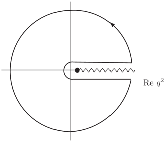
Figure 1: Analytic structure of $\Pi^{(1+0)}(q^{2})$ in the complex $s=q^{2}$ plane. There is a cut on the positive real axis starting at $s=q^{2}=4m_{\pi}^{2}$ (a pole at $s=q^{2}=m_{\pi}^{2}$ and a cut starting at $s=9m_{\pi}^{2}$) for the $V$ ($A$) case. The solid curve shows the contour used in Eq. (3).

The flavor-$ud$ $V$ and $A$ spectral functions can be experimentally determined from the differential versions of the ratios

$$R_{V/A;ud}={\frac{\Gamma[\tau\rightarrow({\rm hadrons})_{V/A;ud}\nu_{\tau}(\gamma)]}{\Gamma[\tau\rightarrow e\bar{\nu}_{e}\nu_{\tau}(\gamma)]}}\ ,$$ (4)

of the hadronic decay width induced by the relevant current to that for the electron mode. Explicitly [31],

$${\frac{dR_{V/A;ud}(s)}{ds}}=12\pi^{2}|V_{ud}|^{2}S_{EW}\,{\frac{1}{m_{\tau}^{2}}}\left[w_{T}(s;m_{\tau}^{2})\rho_{V/A;ud}^{(1+0)}(s)-w_{L}(s;m_{\tau}^{2})\rho_{V/A;ud}^{(0)}(s)\right]\ ,$$ (5)

where $S_{EW}$ is a short-distance electroweak correction and

$$w_{T}(s;s_{0}) = \left(1-\frac{s}{s_{0}}\right)^{2}\left(1+2\,\frac{s}{s_{0}}\right)\ ,$$ (6)

$$w_{L}(s;s_{0}) = 2\,\frac{s}{s_{0}}\left(1-\frac{s}{s_{0}}\right)^{2}\ .$$

With the exception of the known pion-pole part of $\rho_{A;ud}^{(0)}$, the spectral functions $\rho_{V/A;ud}^{(0)}$ are chirally suppressed, $\rho_{V/A;ud}^{(0)}(s)=O[(m_{d}\mp m_{u})^{2}]$, and can be neglected in the non-strange case. The spectral functions $\rho^{(1+0)}_{V/A;ud}(s)$ can thus be determined directly from $dR_{V/A;ud}(s)/ds$ for any positive value of $s\leq m_{\tau}^{2}$, allowing us to apply the FESR (3) for arbitrary $s_{0}\leq m_{\tau}^{2}$ and arbitrary analytic weight $w(s)$ to the data. As in Ref. [9], we will denote the experimental spectral integral on the left-hand side of Eq. (3) by $I_{V/A;\rm ex}^{(w)}(s_{0})$ and the theoretical representation of the contour integral on the right-hand side by $I_{V/A;\rm th}^{(w)}(s_{0})$.

For large enough $|s|=s_{0}$, and sufficiently far away from the positive real axis, $\Pi^{(1+0)}(s)$ can be approximated by the OPE

$$\Pi^{(1+0)}_{\rm OPE}(z)=\sum_{k=0}^{\infty}\frac{C_{2k}(z)}{(-z)^{k}}\ ,$$ (7)

where the logarithmic $z$ dependence of the OPE coefficients $C_{2k}$ can be calculated in perturbation theory.

For the $k=0$ term, it is convenient to consider, instead of $\Pi(z)$, the Adler function $D(z)\equiv-z\,d\Pi(z)/dz$, which is finite and independent of the renormalization scale $\mu$. Accordingly, the $k=0$ contribution to the right-hand side of Eq. (3) can be expressed in terms of the Adler function via partial integration. The $k=0$ contribution $D_{0}(z)$ to $D(z)$ takes the form

$$D_{0}(z)\equiv-z\,\frac{dC_{0}(z)}{dz}=\frac{1}{4\pi^{2}}\sum_{n=0}^{\infty}\left(\frac{\alpha_{s}(\mu^{2})}{\pi}\right)^{n}\sum_{m=1}^{n+1}mc_{nm}\left(\log\frac{-z}{\mu^{2}}\right)^{m-1}\ ,$$ (8)

where the coefficients $c_{nm}$ are known to order $\alpha_{s}^{4}$ [2]. The independence of $D_{0}(z)$ on $\mu$ implies that only the coefficients $c_{n1}$ are independent; the $c_{nm}$ with $m>1$ can be expressed in terms of $c_{n1}$ through use of the renormalization group. In the $\overline{\rm MS}$ scheme, $c_{01}=c_{11}=1$, $c_{21}=1.63982$, $c_{31}=6.37101$ and $c_{41}=49.07570$, for three flavors [2]. While $c_{51}$ is not known at present, we will use the estimate $c_{51}=283$ of Ref. [33], with a 50% uncertainty. For the running of $\alpha_{s}$ we use the four-loop $\overline{\rm MS}$ $\beta$-function, but we have checked that using five-loop running instead [34, 35] leads to differences of order $10^{-4}$ or less in our results for $\alpha_{s}(m_{\tau})$.

The $C_{2k}$ with $k\geq 1$ are different for the $V$ and $A$ channels, and, for $k>1$, contain non-perturbative $D=2k$ condensate contributions. As in Refs. [12, 13], we will neglect purely perturbative quark-mass contributions to $C_{2k}$, $k\geq 1$, as they are numerically very small for the non-strange FERSs we consider in this paper. We will also neglect the $z$-dependence of the coefficients $C_{2k}$ for $k>1$. For a more detailed discussion of our treatment of the $D>0$ OPE contributions, we refer to Ref. [12].

Perturbation theory, and in general the OPE, breaks down near the positive real $s=q^{2}$ axis [36]. If this were not the case, Eq. (3) would establish a direct correspondence between the OPE and the resonant behavior of the experimental spectral function, generally referred to as quark-hadron duality. We account for the breakdown of this duality by replacing the right-hand side of Eq. (3) by

$$-\frac{1}{2\pi is_{0}}\oint_{|z|=s_{0}}dz\,w(z)\,\left(\Pi^{(1+0)}_{\rm OPE}(z)+\Delta(z)\right)\ ,$$ (9)

with

$$\Delta(z)\equiv\Pi^{(1+0)}(z)-\Pi^{(1+0)}_{\rm OPE}(z)\ ,$$ (10)

where $\Delta(z)\equiv\Delta_{V/A}(z)$ defines the quark-hadron duality violating contribution to $\Pi^{(1+0)}(z)\equiv\Pi_{V/A}^{(1+0)}(z)$. If $\Delta(z)$ decays fast enough for $|z|\to\infty$, Eq. (9) can be rewritten as [37]

$$I_{\rm th}^{(w)}(s_{0})=-\frac{1}{2\pi is_{0}}\oint_{|s|=s_{0}}dz\,w(z)\,\Pi^{(1+0)}_{\rm OPE}(z)-\frac{1}{s_{0}}\,\int_{s_{0}}^{\infty}ds\,w(s)\,\frac{1}{\pi}\,\mbox{Im}\,\Delta(s)\ .$$ (11)

The imaginary parts $\frac{1}{\pi}\,\mbox{Im}\,\Delta_{V/A}(s)$ can be interpreted as the duality-violating parts $\rho_{V/A}^{\rm DV}(s)$ of the $V/A$ spectral functions, and represent the resonance-induced, oscillatory parts of the spectral functions not captured by the OPE.

In Ref. [25], we developed a theoretical framework for quark-hadron duality violations in terms of a generalized Borel–Laplace transform of $\Pi(q^{2})$ and hyperasymptotics, building on earlier work [38, 39, 40, 41]. In the chiral limit, and assuming that for high energies the spectrum becomes Regge-like in the $N_{c}\to\infty$ limit, we showed that the asymptotic form of $\rho_{V/A}^{\rm DV}(s)$ for large $s$ can be parametrized as

$$\rho_{V/A}^{\rm DV}(s)=\frac{1}{\pi}\,\mbox{Im}\,\Delta_{V/A}(s)=e^{-\delta_{V/A}-\gamma_{V/A}s}\sin(\alpha_{V/A}+\beta_{V/A}s)\ ,$$ (12)

up to slowly varying logarithmic corrections in the argument of the sine factor, and with $\gamma\sim 1/N_{c}$ small but non-zero. The parameters $\beta_{V/A}$ are directly related to the Regge slopes in the $V$ and $A$ channels, and the parameters $\gamma_{V/A}$ to the (asymptotic) ratio of the width and the mass of the resonances in those channels. While the framework of Ref. [25] is rather general, and the derivation of Eq. (12) is based on generally accepted conjectures about QCD (primarily Regge behavior), it does not provide a derivation from first principles. This introduces a certain model dependence in our analysis which, however, can be tested by fits to the data. Such tests, in particular, will provide information about the values of $s$ above which this asymptotic form is likely to be sufficiently accurate. We emphasize, however, that modifications to the parametrization of Eq. (12) are constrained by the general framework of Ref. [25].

Equation (12) introduces, in addition to $\alpha_{s}$ and the $D\geq 4$ OPE condensates, four new parameters in each channel: $\delta_{V/A},\gamma_{V/A},\alpha_{V/A}$ and $\beta_{V/A}$. This can be compared to the truncated-OPE approach in which DVs are neglected. Since resonance-induced oscillations are clearly visible in the experimental spectral data, and their dynamical effect is comparable in size to the $\alpha_{s}$-dependent dynamical effect of perturbative corrections to the ($\alpha_{s}$-independent) parton model contribution [26], this approach also assumes a model: one in which the parameters $\delta_{V/A}$ are effectively set to infinity by hand. This is a stronger assumption, and one that has been shown to fail a number of subsequent, more stringent data-based tests [26, 27].

In summary, as in Refs. [12, 13], we will assume that Eq. (12) holds for $s\geq s_{\rm min}$, with $s_{\rm min}$ to be determined from fits to the data. This assumes of course that the $s_{\rm min}$ for which this assumption is valid includes a region below $m_{\tau}^{2}$, i.e., that both the OPE (7) and the DV parametrization (12) can be used in some interval below $m_{\tau}^{2}$.

II.2 Choice of weight functions and the OPE

The logarithmic $s$ dependence of the OPE coefficients $C_{D}(s)$ is calculable in perturbation theory. Because the running of $\alpha_{s}$ becomes visible only at non-leading order in $\alpha_{s}$, this $s$ dependence is an ${\cal O}(\alpha_{s}^{2})$ effect in the chiral limit. Such effects were found to be safely negligible for $D>0$ in the sum-rule analysis of the OPAL data reported in Ref. [12], and we will thus ignore them for $D>0$ in the present analysis as well. With this simplification, a term in a weight $w(z)$ proportional to the monomial $z^{n}$ picks out the $D>0$ OPE contribution with $D=2k=2(n+1)$ in the sum rule (3). The choice of a polynomial weight $w(z)$ thus projects the sum rule on a finite number of $D>0$ terms in the OPE.

In this paper, we will consider the weights $w(z)=w_{n}(z/s_{0})$ with

$$w_{0}(y) = 1\ ,$$ (13)

$$w_{2}(y) = 1-y^{2}\ ,$$

$$w_{3}(y) = (1-y)^{2}(1+2y)\ ,$$

$$w_{4}(y) = (1-y^{2})^{2}\ ,$$

where the subscript indicates the degree of the polynomial. These weights explore OPE terms with $D\leq 10$, and form a linearly independent basis for polynomials up to degree four without a linear term. The weight $w_{0}(y)$ projects only the $D=0$ term of the OPE (i.e., pure perturbation theory), the weight $w_{2}(y)$ projects, in addition, $D=6$, $w_{3}(y)$ projects $D=0$, $D=6$ and $D=8$, while $w_{4}(y)$ projects $D=0$, $D=6$ and $D=10$. As the OPE itself diverges as an expansion in $1/z$, it is safer to include sum rules with low-degree weights such as $w_{0}(y)$ and $w_{2}(y)$ in the analysis, and check for consistency among sum rules with different weights. We note that $w_{3}(s/s_{0})=w_{T}(s;s_{0})$, cf.   Eq. (6).

None of these weights contain a term linear in $z$, and thus the $D=4$ OPE term does not contribute to the sum rules with these weights. This choice is motivated by the results of Ref. [44], in which a renormalon-model-based study suggested that perturbation theory is particularly unstable for sum rules with weights containing such a linear term.

The weights $w_{2,3,4}(y)$ are “pinched,” i.e., they have zeroes at $z=s_{0}$, and thus suppress contributions from the region near the timelike point $z=s_{0}$ on the contour, and hence also the relative importance of integrated DV contributions [46, 47]. The weight $w_{2}(y)$ has a single zero at $z=s_{0}$ (a single pinch), while the weights $w_{3}(y)$ and $w_{4}(y)$ are doubly pinched, i.e., have a double zero at $z=s_{0}$.

II.3 Perturbative uncertainties and FOPT vs. CIPT

It has become common practice to consider different resummations of perturbation theory in order to obtain insight into the effect of neglecting terms beyond those explicitly included in evaluating the $D=0$ (i.e., perturbative) contribution to the right-hand side of Eq. (3). The two most commonly used resummation prescriptions are fixed-order perturbation theory (FOPT), in which the scale $\mu$ in Eq. (8) is chosen to be fixed at $\mu^{2}=s_{0}$, and contour-improved perturbation theory (CIPT) [29, 30], a partial resummation obtained by choosing $\mu^{2}$ equal to $-z$ point by point along the contour. In the CIPT prescription, the coupling is run along the contour $|z|=s_{0}$, using the four- (or five-)loop beta function; as a result, only terms with $m=1$ survive in Eq. (8). The two prescriptions lead to significantly different values of $\alpha_{s}$, with the difference being comparable to the combination of all other errors [9, 13], but more significant, since the results obtained with different prescriptions using the same data are highly correlated.

The choice of such a prescription is entangled with the choice of renormalization scheme, since the choice of scheme also affects higher orders in perturbation theory. Both FOPT and CIPT prescriptions are usually considered to be $\overline{\rm MS}$ schemes, but clearly, if the choice between FOPT and CIPT is rephrased as a choice of scheme, these two schemes are different. Since $\alpha_{s}$ is not a physically measurable quantity, ideally, one would like to choose a scheme, and a prescription, which corresponds to the scheme chosen to quote other determinations of $\alpha_{s}$ (such as that from $Z$ decay itself), so that a direct comparison is possible at $M_{Z}$.

In our case, the experimental quantities from which we determine $\alpha_{s}$ are the spectral integrals $I^{(w)}_{\rm ex}(s_{0})$, in which $s_{0}$ is varied between $s_{0}=s_{\rm min}$ and $s_{0}=m_{\tau}^{2}$. Apart from DVs, which appear in a transseries beyond the OPE, these quantities are then expressed in terms of the OPE, which at $D=0$ is parametrized by $\alpha_{s}(\mu)$ and the ratio of scales $s_{0}/\mu^{2}$, while at $D\geq 4$ also the condensates enter. This leads to the theoretical representations $I^{(w)}_{\rm th}(s_{0},s_{0}/\mu^{2},\alpha_{s}(\mu))$, which are then to be equated with $I^{(w)}_{\rm ex}(s_{0})$. Since $I^{(w)}_{\rm ex}(s_{0})$ is an observable with a single physical scale, $s_{0}$, the natural choice is to choose the scale $\mu$ equal to the scale of the observable, i.e., to choose $\mu^{2}=s_{0}$. This corresponds directly to the way the scale is chosen for other determinations of $\alpha_{s}$. For instance, the hadronic $Z$-decay rate can be expressed perturbatively in terms of $\alpha_{s}(\mu)$ in the $\overline{\rm MS}$ scheme, and in that case, the natural choice of scale is $\mu=M_{Z}$. This leads us to conclude that, in the case of hadronic $\tau$ decays, the prescription most directly comparable with other determinations is FOPT. We emphasize that we do not claim to know which prescription, at a given order, gives the best approximation to the QCD answer for $I^{(w)}_{\rm ex}(s_{0})$. This may depend on the weight $w$, and on the order in perturbation theory [44]. The point is to choose a scheme that corresponds most closely to the scheme employed in other determinations of $\alpha_{s}$ at the $Z$-mass. Of course, it is necessary to estimate the systematic uncertainty inherent in the truncation of perturbation theory, and we will return to this point at the end of this subsection.

Before we do this, we present an additional reason for using FOPT as the prescription to be used in the FESR determination of $\alpha_{s}$ from hadronic $\tau$ decays. It is well known that perturbation theory for the Adler function, and for the quantities $I^{(w)}_{\rm th}(s_{0})$, is not convergent. Attempts to go beyond perturbation theory using Borel resummation techniques lead to ambiguities in the Borel sum that necessitate the introduction of $D>0$ terms in the OPE [48]. The most well-known example is that of the leading infrared renormalon in massless QCD. This leads to the $D=2k=4$ term in Eq. (7), which removes the ambiguity associated with this renormalon. The appearance of $D>0$ terms in Eq. (7) is thus intricately connected to resummations of perturbation theory.

In Ref. [49], it was shown that, in general, the FOPT and CIPT series lead to different Borel sums, with different analytical properties. Moreover, it was pointed out that this different analytical behavior of the Borel sums for $I^{(w)}_{\rm th}(s_{0})$ appears to invalidate the correspondence between infrared renormalons and the $D>0$ terms in the OPE in the case of CIPT. The Borel sum for the CIPT series does not allow for the usual renormalon ambiguities that in the case of FOPT are in one-to-one correspondence with terms in the OPE. Thus, there is a mismatch between the use of CIPT, and the representation of $\Pi^{(1+0)}(z)$ by the OPE, Eq. (7). This mismatch between the Borel sum and the OPE does not happen in FOPT.

This observation casts strong doubts on the consistency of using the OPE (7) in the case of CIPT. Again, this does not settle the issue of whether the (Borel sum of) FOPT or CIPT provides a better approximation to QCD. But it does imply that it is theoretically inconsistent to apply the OPE in the form (7) if one uses CIPT in the evaluation of the $D=0$ perturbative contributions, and therefore casts doubts on all CIPT-based extractions of $\alpha_{s}$. We are thus led to the conclusion that FOPT should be taken as the preferred choice for analyzing hadronic $\tau$ decays using the OPE. While we will provide determinations of $\alpha_{s}(m_{\tau})$ employing both FOPT and CIPT (ignoring the OPE subtleties in the case of CIPT) we will quote the FOPT value as our final result, to be compared with other $\overline{\rm MS}$ determinations of $\alpha_{s}$. We will also give a CIPT value based on fits to $I^{(w)}_{\rm ex}(s_{0})$, allowing the reader to compare to earlier CIPT results and assess the impact of changes in the input inclusive $V$ spectral function.

We will determine the systematic error associated with the use and truncation of perturbation theory for our FOPT value of $\alpha_{s}(m_{\tau})$ as follows. First, as already indicated in Sec. II.1, we will vary the estimated value for $c_{51}=283$ by plus or minus 50%. This interval for $c_{51}$ includes all estimates available in the literature by a rather wide margin. The variation by $\pm 50\%$ was proposed in Ref. [33], and the estimate of Ref. [2] falls well inside this interval. Subsequent estimates of both the central value and the uncertainty of $c_{51}$ are also generously covered by the $\pm 50\%$ variation [50, 51]. This choice of range, of course, provides an estimate only for the impact of the uncertainty in the value of the unknown coefficient $c_{51}$, and might constitute an underestimate of the total perturbative error. At present, the perturbative expansion for the Adler function has been calculated to order $\alpha_{s}^{4}$. An alternate, potentially more conservative, estimate of the perturbative error can thus also be obtained by omitting the ${\cal O}(\alpha_{s}^{4})$ contribution altogether, i.e., by setting $c_{4m}=0$ (as well as $c_{nm}=0$ for all $n>4$) in Eq. (8). Finally, since our FOPT determination employs a range of $s_{0}$ varying between $s_{\rm min}$ and $m_{\tau}^{2}$, a third sensible estimate of the perturbative error can be obtained by considering, instead of just $\mu^{2}=s_{0}$, also the alternate choices $\mu^{2}=s_{\rm min}$, $\mu^{2}=m_{\tau}^{2}$ and $\mu^{2}=2s_{0}$ for the scale $\mu$. We will take the largest of the variations in $\alpha_{s}$ obtained by applying all three methods above as our best estimate for the systematic error associated with the necessary truncation of perturbation theory. We do not combine the errors obtained by using these three methods, as this would correspond to a double-counting of the estimated perturbative uncertainties. We will, however, add an independent measure of the uncertainty associated with the use of perturbation theory based on the comparison of the central values obtained from fits with different weights, as explained in more detail in Sec. IV.3.

III Data

In this section, we construct an updated version of the inclusive, non-strange $V$ spectral function, $\rho_{ud;V}(s)$, using publicly available ALEPH [3, 4, 5, 52] and OPAL [6] $\tau$ data for the contributions of the dominant $2\pi$ and $4\pi$ exclusive modes, recent BaBar $\tau$-decay results [53] for the contribution of the $K^{-}K^{0}$ mode, and $e^{+}e^{-}\rightarrow hadrons$ cross section data as input to CVC evaluations of the contributions of the remaining exclusive modes.

In Refs. [3, 4, 5, 6], the inclusive $V$ and $A$ invariant-mass-squared distributions were constructed as sums of (i) the measured (and publicly available) distributions for the main exclusive modes in the channel and (ii) the sum of small contributions from the remaining “residual” exclusive modes. The publicly available exclusive-mode distributions are normalized to then-current exclusive-mode BFs. While the accompanying inclusive-sum correlation matrices include the contributions from then-current exclusive-mode BF uncertainties and correlations for the main exclusive modes, the exclusive-mode correlation matrices are provided with the BF-uncertainty-induced contributions omitted, allowing subsequently improved BF information for these modes to be incorporated at a later time.

The $V$ channel modes for which ALEPH and OPAL provide exclusive-mode distribution and correlation information are $\pi^{-}\pi^{0}$, $\pi^{-}3\pi^{0}$ and $\pi^{-}\pi^{+}\pi^{-}\pi^{0}$. For the $A$ channel, ALEPH provides distribution and correlation information for only the two $3\pi$ modes, $2\pi^{-}\pi^{+}$ and $\pi^{-}2\pi^{0}$, while OPAL provides this information, in addition, for one of the three $5\pi$ modes, $2\pi^{-}\pi^{+}2\pi^{0}$. While all exclusive-mode distributions are normalized to then-current values of the corresponding exclusive-mode BFs, the $s$-dependences of some of the residual-mode distributions are taken from Monte Carlo. For OPAL, this is true for all but the $\pi^{-}\pi^{0}\omega(\rightarrow{\rm\mbox{non-}3}\pi)$ residual $A$ mode. For ALEPH, the use of the Monte Carlo simulations is explicitly identified as entering the $6\pi$, $K^{-}K^{0}$, $K\bar{K}\pi\pi$ and $\pi^{-}\omega(\rightarrow{\rm\mbox{non-}3}\pi)$ contributions to the $V$ channel and the $K\bar{K}\pi$ and $K\bar{K}\pi\pi$ contributions to the $A$ channel. Since the information made publicly available by ALEPH and OPAL does not include the individual BF-normalized residual exclusive-mode distributions used by the collaborations in determining their final inclusive-sum results, it is not possible to update those residual-mode contributions to reflect subsequent improvements in our knowledge of the exclusive-mode BFs and/or new information on the $s$-dependence of exclusive-mode distributions for which Monte Carlo was previously employed. Improvements to the residual-mode contributions must, therefore, come from other sources. The dominant $V$ and $A$ channel modes (those for which both ALEPH and OPAL exclusive-mode distributions are available) represent 98.0% of the inclusive $V$ channel BF and 94.2% of the continuum inclusive $A$ channel BF.

Improving the treatment of residual-mode contributions is much easier for the $V$ channel than for the $A$ channel. The reason is that, strongly motivated by the drive to improve the determination of the Standard-Model hadronic vacuum polarization contribution to the anomalous magnetic moment of the muon, there has been an intensive program of collider and $B$-factory experiments aimed at determining the $e^{+}e^{-}\rightarrow hadrons$ cross-sections for all exclusive modes contributing to the inclusive $R(s)$ ratio in the region below $s\simeq 4$ GeV². A sizeable fraction of these exclusive modes can be uniquely classified as either $I=0$ or $I=1$ using $G$-parity. The CVC relation between the bare cross section for the electroproduction of the neutral member, $X^{0}$, of the exclusive-mode isotriplet $X$, $\sigma^{b}_{X}(s)\equiv\sigma^{b}[e^{+}e^{-}\rightarrow X^{0}]$, and the contribution of the charged isospin partner, $X^{-}$, to $\rho_{ud;V}(s)$,

$$\left[\rho_{ud;V}(s)\right]_{X^{-}} = {\frac{s\,\sigma^{b}_{X}(s)}{8\pi^{3}\alpha_{EM}^{2}}}$$ (14)

then allows the cross section results for those exclusive residual modes with $I=1$ to be used to determine the corresponding exclusive residual-mode contributions to $\rho_{ud;V}(s)$. Eq. (14) is valid up to isospin-breaking (IB) corrections which, in the absence of narrow interfering resonances, should be of the order a percent or so, and hence numerically negligible on the scale of the experimental errors on the already small residual-mode contributions. This strategy, of using CVC to improve the determination of an otherwise poorly determined $V$ exclusive-mode $\tau$ spectral function contribution, was pioneered by ALEPH [52], which used the BaBar Dalitz-plot-analysis separation of $I=0$ and $I=1$ contributions to the $e^{+}e^{-}\rightarrow K\bar{K}\pi$ cross sections [54] to determine the $V$ part of the $\tau\rightarrow K\bar{K}\pi\nu_{\tau}$ distribution, and hence the separation of that distribution into its $V$ and $A$ components. The CVC relation allows us to dramatically improve the vast majority of the residual-mode contributions to the $V$ spectral function. This is especially helpful in the case of contributions from higher-multiplicity modes, whose $\tau$-decay distributions lie at higher $s$, increasingly close to the $\tau$ kinematic endpoint, and with, as a result, increasingly reduced statistical precision.

The main $V$ residual mode for which such a CVC improvement is not possible is $K^{-}K^{0}$, where the $e^{+}e^{-}\rightarrow K\bar{K}$ cross sections contain both $I=0$ and $I=1$ contributions, and it is not possible to identify only the $I=1$ component. Fortunately, for this channel, BaBar [53] has recently published a rather precise determination of the unit-normalized $\tau\rightarrow K^{-}K_{S}\nu_{\tau}$ number distribution, allowing the residual-mode $K^{-}K^{0}$ contribution to $\rho_{ud;V}(s)$, to be determined directly, without the use of CVC.

Using CVC and the recent BaBar $\tau$ $K^{-}K^{0}$ results, 99.95% by BF of the inclusive $V$ spectral function can be determined directly from experiment. The remaining $0.05\%$ represents only 2.4% by BF of the already small sum of residual-mode contributions. CVC improvements are, of course, impossible for $A$ channel residual-mode distributions. This, and the larger relative role played by residual-mode contributions in the $A$ channel, are the primary reasons for our focus on the $V$ channel in this paper.

The rest of this section is organized as follows. First, in Sec. III.1, we specify the sources of external input employed in our update of $\rho_{ud;V}(s)$. Next, in Sec. III.2, we outline the procedure used for combining the publicly available data from ALEPH and OPAL for the dominant $2\pi$ and $4\pi$ exclusive-modes, following closely that described in Ref. [14] for combining exclusive-mode $e^{+}e^{-}$ cross sections from different experiments. Details of our updates of the individual residual exclusive-mode contributions are provided in Sec. III.3. Finally, the resulting updated version of $\rho_{ud;V}(s)$, is presented in Sec. III.4.

III.1 External input

As noted above, we employ publicly available results for the non-residual ($\pi^{-}\pi^{0}$, $\pi^{-}3\pi^{0}$ and $\pi^{-}\pi^{+}\pi^{-}\pi^{0}$) exclusive-mode distributions and correlations provided by the ALEPH [3, 4, 5, 52] and OPAL [6] collaborations.

ALEPH quotes results in the form of exclusive-mode, BF-normalized contributions, $dB_{X}(s)/ds$, to the differential BF distribution $dB(s)/ds$. The corresponding contributions to $\rho_{ud;V}(s)$, $\rho^{X}_{ud;V}(s)$, follow from

$$\rho^{X}_{ud;V}(s)\, =\,{\frac{m_{\tau}^{2}}{12\pi^{2}B_{e}S_{\rm EW}|V_{ud}|^{2}w_{T}(s;m_{\tau}^{2})}}\,{\frac{dB_{X}(s)}{ds}}$$ (15)

$$=\,{\frac{B_{X}m_{\tau}^{2}}{12\pi^{2}B_{e}S_{\rm EW}|V_{ud}|^{2}w_{T}(s;m_{\tau}^{2})}}\,{\frac{1}{N_{X}}}{\frac{dN_{X}(s)}{ds}}$$

where $B_{X}$ is the BF for exclusive mode $X$, ${\frac{1}{N_{X}}}{\frac{dN_{X}(s)}{ds}}$ is the corresponding experimental unit-normalized number distribution, and $B_{e}$ is the $\tau^{-}\rightarrow e^{-}\nu_{\tau}\bar{\nu}_{e}$ BF. ALEPH results for $dB_{X}(s)/ds$ are updated by rescaling to the current value of $B_{X}$. Current values of the external parameters, $B_{e}$, $S_{\rm EW}$, $V_{ud}$ and $m_{\tau}$ are then used to obtain the updated results for $\rho^{X}_{ud;V}(s)$.

OPAL quotes results in the form of the exclusive-mode contributions $\rho^{X}_{ud;V}(s)$. These were obtained from the experimentally measured unit-normalized number distributions via Eq. (15), using then-current values of the exclusive-mode BFs, $B_{X}$, and the external inputs $B_{e}$, $S_{\rm EW}$, $V_{ud}$ and $m_{\tau}$. The underlying unit-normalized distributions are reconstituted using the values for the exclusive-mode BFs and external inputs quoted by OPAL, and converted to equivalent updated versions of the $\rho^{X}_{ud;V}(s)$ using current values for these inputs.

We employ the following values for the external parameters appearing in Eq. (15): for $B_{e}$, the lepton-universality-improved HFLAV 2019 [55] result $B_{e}=0.17814(22)$; for $m_{\tau}$ and $|V_{ud}|$, the PDG 2020 [56] results $m_{\tau}=1.77686(12)$ GeV and $|V_{ud}|=0.97370(14)$; and, for $S_{\rm EW}$, the result $S_{\rm EW}=1.0201(3)$ [57].

For the exclusive-mode BFs and the correlations between them we employ HFLAV 2019 [55] results. Note that HFLAV quotes a result for the $\pi^{-}\pi^{+}\pi^{-}\pi^{0}$ BF which excludes $K^{0}$ contributions but not the small “wrong-current” $A$ $\pi^{-}\pi^{0}\omega(\rightarrow\pi^{+}\pi^{-})$ contribution. The $V$ part of the $\pi^{-}\pi^{+}\pi^{-}\pi^{0}$ BF is obtained by removing this $A$ “contamination” using the HFLAV $\pi^{-}\pi^{0}\omega$ BF and 2020 PDG [56] result for the IB $\omega\rightarrow\pi^{-}\pi^{+}$ BF. Similar wrong-current corrections are made to the correlations between the BFs.

Specifics of the experimental inputs used in the determination of the residual-mode contributions to $\rho_{ud;V}(s)$ are detailed in Sec. III.3 below.

III.2 Combining the ALEPH and OPAL $2\pi$ and $4\pi$ data

We begin with the updated versions of the ALEPH and OPAL exclusive-mode distributions, $\rho^{X}_{ud;V}(s)$, with $X=\pi^{-}\pi^{0}$, $\pi^{-}3\pi^{0}$ and $\pi^{-}\pi^{+}\pi^{-}\pi^{0}$, obtained as outlined in the previous subsection. Ideally, we would like to combine the results for each of these exclusive modes separately, first combining the ALEPH and OPAL unit-normalized number distributions (which are independent of the BFs) and then multiplying the resulting combined exclusive distributions by the corresponding BFs. It turns out, however, that this is not possible. The reason is that the correlation matrices for the $\pi^{-}3\pi^{0}$ and $\pi^{-}\pi^{+}\pi^{-}\pi^{0}$ distributions for both experiments have zero eigenvalues, i.e., 100% correlations between different bins, and hence are not invertible. This prevents us from combining the ALEPH and OPAL data for the individual $4\pi$ modes in the manner described below. If, however, we first sum the contributions from all three modes, we find that the correlation matrices for the resulting three-mode-sums are well behaved for both ALEPH and OPAL. We thus combine the ALEPH and OPAL exclusive-mode results by first summing, for each experiment separately, the contribution to $\rho_{ud;V}(s)$ and the corresponding covariance matrices from $\pi^{-}\pi^{0}$, $\pi^{-}3\pi^{0}$ and $\pi^{-}\pi^{+}\pi^{-}\pi^{0}$, using updated versions of the exclusive-mode BFs, and then combining those results using the method outlined below.

Following Ref. [14], we choose a number of clusters, distributed over the interval $0<s\leq m_{\tau}^{2}$. We assign a number of consecutive ALEPH and OPAL data points to each cluster $m$, $m=1,\dots,N_{\rm cl}$, with $N_{\rm cl}$ the total number of clusters; $N_{m}$ will be the total number of data points in cluster $m$. If the collective ALEPH and OPAL data points are parametrized by pairs $(s_{i},d_{i})$, where $d_{i}$ is the ALEPH or OPAL data point for the spectral function assigned to the $s$-value $s_{i}$, we define weighted cluster averages

$$s^{(m)}=\sum_{i\in m}\frac{s_{i}}{\sigma^{2}_{i}}\Bigg{/}\sum_{i\in m}\frac{1}{\sigma^{2}_{i}}\ ,$$ (16)

where the sum is over all data points in cluster $m$ and $\sigma^{2}_{i}$ is the variance of $d_{i}$, i.e., the $\sigma^{2}_{i}$ are the diagonal elements of the covariance matrix $C_{ij}$ for the spectral-function data points $d_{i}$. The set of $s^{(m)}$ then constitutes the values of $s$ at which the combined spectral function $\rho^{(m)}$ will be defined.

The values of $\rho^{(m)}$ will be determined by linear interpolation, minimizing

$$\chi^{2}(\rho)=\sum_{i=1}^{N}\sum_{j=1}^{N}\left(d_{i}-R(s_{i};\rho)\right)C^{-1}_{ij}\left(d_{j}-R(s_{j};\rho)\right)\ ,$$ (17)

where $N=\sum_{m=1}^{N_{\rm cl}}N_{m}$ is the total number of (ALEPH and OPAL) data points, and the piece-wise linear function $R(s;\rho)$ is defined by

$$R(s;\rho)=\rho^{(m)}+\frac{s-s^{(m)}}{s^{(m+1)}-s^{(m)}}\left(\rho^{(m+1)}-\rho^{(m)}\right)\ ,\quad s^{(m)}\leq s\leq s^{(m+1)}\ ,\quad 1\leq m<N_{\rm cl}\ ,$$ (18)

where $\rho$ is the vector of fit parameters $\rho^{(m)}$, $m=1,\dots,N_{\rm cl}$. At the boundaries, we extrapolate:

$$R(s;\rho) = \rho^{(N_{\rm cl}-1)}+\frac{s-s^{(N_{\rm cl}-1)}}{s^{(N_{\rm cl})}-s^{(N_{\rm cl}-1)}}\left(\rho^{(N_{\rm cl})}-\rho^{(N_{\rm cl}-1)}\right)\ ,\qquad s\geq s^{(N_{\rm cl})}\ ,$$ (19)

$$R(s;\rho) = \rho^{(1)}+\frac{s-s^{(1)}}{s^{(2)}-s^{(1)}}\left(\rho^{(2)}-\rho^{(1)}\right)\ ,\qquad\qquad\qquad\qquad\ s\leq s^{(1)}\ .$$

Minimizing $\chi^{2}(\rho)$ yields the linear equations

$$\sum_{i=1}^{N}\sum_{j=1}^{N}\left(d_{i}-R(s_{i};\rho)\right)C^{-1}_{ij}\,\frac{\partial R(s_{j};\rho)}{\partial\rho^{(m)}}=0\ ,\qquad 1\leq m\leq N_{\rm cl}\ ,$$ (20)

which can be solved for the $\rho^{(m)}$, with the cluster covariance matrix ${\cal C}_{mn}$ given by

$${\cal C}_{mn}^{-1}=\sum_{i=1}^{N}\sum_{j=1}^{N}\frac{\partial R(s_{i};\rho)}{\partial\rho^{(m)}}\,C^{-1}_{ij}\,\frac{\partial R(s_{j};\rho)}{\partial\rho^{(n)}}\ .$$ (21)

The procedure for combining exclusive spectral functions followed in Ref. [14] is more complicated than the one outlined above. The inclusion of uncertainties in the BFs in the covariance matrices can lead to a bias in the fit [58], and the method employed in Ref. [14] adjusts for this bias [59]. However, for this to work, we would need to combine each channel separately, because multiplication by the exclusive-mode BF is needed in each channel to turn the normalized distribution into the corresponding contribution to $\rho_{ud;V}(s)$. This path is not available to us, because, as explained above, only the sum of the $\pi^{-}\pi^{0}$, $\pi^{-}3\pi^{0}$ and $\pi^{-}\pi^{+}\pi^{-}\pi^{0}$ spectral distributions can be combined. This sum incorporates three different branching fractions, one for each exclusive channel. The effect of the BF uncertainties is, however, very small numerically. We have checked that their inclusion changes central values of the combined three-mode contribution to $\rho_{ud;V}(s)$ by less than 0.5%, while the errors on this contribution are about one percent larger with than without inclusion of BF uncertainties, and the cluster values $s^{(m)}$ are essentially unaffected. It is thus safe to ignore potential bias issues associated with the incorporation of BF uncertainties. The same is true for the impact of the uncertainties in the external normalizing factors $V_{ud}$, $S_{\rm EW}$, and $B_{e}$. The errors on $V_{ud}$ and $S_{\rm EW}$ are completely negligible, while the error on $B_{e}$, at about 0.1% is small enough that it does not lead to a discernible bias.

In order to obtain an optimal combined data set, one needs to choose the clusters judiciously. Clearly, the maximum number of clusters one can choose is equal to the sum of the total number of ALEPH and OPAL data points. However, such a choice is not useful. One would find a $\chi^{2}$ per degree of freedom (dof) much smaller than one, but this is not what one expects if one averages two independent experiments. Since both ALEPH and OPAL measured the spectral function over the same range in $s$, the number of clusters should be chosen not larger than the number of data points in each of the experiments, and, given that these two experiments are independent, one expects a $\chi^{2}/$dof of order one. The goal is thus to choose a set of clusters not larger than the number of data points in either experiment that leads to a value of $\chi^{2}(\rho)/\mbox{dof}\approx 1$. Of course, narrower clusters should be used in regions where the spectral function changes rapidly, such as around the $\rho$-meson peak.

In addition to the “global” $\chi^{2}(\rho)$ function defined in Eq. (17), we have also looked at $\chi^{2}_{(m)}$, the “local” $\chi^{2}$ function for each cluster, since the local $\chi^{2}_{(m)}$ values may reveal discrepancies in the data sets that are hidden in the global $\chi^{2}$. The local $\chi^{2}_{(m)}$ is defined as in Eq. (17), but with both the data points $(s_{i},d_{i})$ and the data covariance matrix restricted to those data points contained in cluster $m$. We then evaluate all $\chi^{2}_{(m)}$ on the solution $\rho^{(m)}$, $m=1,\dots,N_{\rm cl}$, obtained by minimizing the global $\chi^{2}(\rho)$. Clearly, the global $\chi^{2}(\rho)$ is not equal to the sum over all clusters of the local $\chi^{2}_{(m)}$, because the full data covariance matrix $C$ contains entries correlating data points in different clusters. If, for a cluster $k$, $\chi^{2}_{(k)}/$dof$>1$, this indicates a fluctuation or a local discrepancy between the ALEPH and OPAL data.

At this stage, we will have obtained a partially-inclusive combined spectral function and associated covariance matrix for the sum of the $\pi^{-}\pi^{0}$, $\pi^{-}3\pi^{0}$ and $\pi^{-}\pi^{+}\pi^{-}\pi^{0}$ modes. We still need to add the residual-mode contributions to obtain our final, updated version of $\rho_{ud;V}(s)$. The determination of the residual-mode contributions is detailed in the next subsection.

III.3 Residual Mode Updates

In this section we provide details of the input used to update the residual exclusive-mode contributions to $\rho_{ud;V}(s)$, i.e., all modes other than $\pi^{-}\pi^{0}$, $\pi^{-}3\pi^{0}$ or $\pi^{-}\pi^{+}\pi^{-}\pi^{0}$. The modes considered in this work are (i) those included in both the OPAL and ALEPH analyses, $\pi^{-}\omega(\rightarrow{\rm\mbox{non-}3}\pi)$, $K^{-}K^{0}$, $\eta\pi^{-}\pi^{0}$, $K\bar{K}\pi$, $3\pi^{-}2\pi^{+}\pi^{0}$, and $2\pi^{-}\pi^{+}3\pi^{0}$, (ii) those included in the ALEPH analysis but not the OPAL analysis, $(3\pi)^{-}\omega(\rightarrow{\rm\mbox{non-}3}\pi)$ and $K\bar{K}\pi\pi$, and (iii) small additional $\pi^{-}5\pi^{0}$ and $\eta\omega\pi+\eta 4\pi$ contributions inferrable from the corresponding $e^{+}e^{-}$ cross sections using CVC, and not included in either of the OPAL or ALEPH analyses.

Note that, where the $e^{+}e^{-}\rightarrow hadrons$ cross sections used to infer, via CVC, the corresponding contributions to $\rho_{ud;V}(s)$, are given in dressed form in the original publications, these have been corrected for vacuum polarization effects to obtain the corresponding bare cross sections required as input to the CVC relation. Statistical and systematic errors on the cross sections are those reported in the relevant references. Additional information, if any, provided by the collaborations is specified below.

All results for $\tau$ exclusive-mode BFs quoted below are obtained using basis-mode BF and correlation information from the 2019 HFLAV compilation [55].

We now turn to a more detailed discussion of the determination of the residual exclusive-mode contributions to $\rho_{ud;V}(s)$. The discussion is organized mode by mode, in the order of decreasing residual-mode BF. Readers interested only in the final result for the inclusive spectral function may skip these details and jump directly to Sec. III.4 below.

III.3.1 The $\pi^{-}\omega(\rightarrow\mbox{non-}3\pi)$ contribution

The $\pi^{-}\omega(\rightarrow{\rm\mbox{non-}3}\pi)$ contribution to $\rho_{ud;V}(s)$ is obtained using CVC, BaBar results [60] for the $e^{+}e^{-}\rightarrow\pi^{0}\omega$ cross sections, and the 2020 PDG value, $0.107(6)$, for the $\omega\rightarrow{\rm\mbox{non-}3}\pi$ BF. The BaBar cross sections are in good agreement with, and have significantly smaller errors than, those reported by SND [61]. The BaBar results produce a CVC prediction of $0.0188(19)$ for the $\tau\rightarrow\pi^{-}\omega\nu_{\tau}$ BF, in excellent agreement with the HFLAV 2019 result, $0.01955(65)$. The contribution to $\rho_{ud;V}(s)$ implied by the BaBar cross sections has been rescaled by the ratio of the HFLAV to the CVC BF to normalize it to the HFLAV 2019 $\tau$ BF. The BF corresponding to the resulting $\pi^{-}\omega(\rightarrow{\rm\mbox{non-}3}\pi)$ contribution to $\rho_{ud;V}(s)$ is $0.00209(14)$.

III.3.2 The $\eta\pi^{-}\pi^{0}$ contribution

The $e^{+}e^{-}\rightarrow\eta\pi^{+}\pi^{-}$ cross sections have been measured by SND [62, 63], BaBar [64, 65] and CMD-3 [66], with the results from all three collaborations in excellent agreement (see, for example, Figure 7 of Ref. [66]). Since CMD-3 has provided us with the corresponding covariances [67], we employ the CMD-3 [66] cross section data as input to our CVC determination of the $\eta\pi^{-}\pi^{0}$ contribution to $\rho_{ud;V}(s)$. As noted by CMD-3, the SND, BaBar and CMD-3 cross sections produce CVC predictions for the $\tau\rightarrow\eta\pi^{-}\pi^{0}\nu_{\tau}$ BF, $0.00156(11)$, $0.00163(8)$ and $0.00168(13)$, respectively, which are in good agreement, but which lie between $1.3$ and $2.3$ $\sigma$ high compared to the corresponding HFLAV 2019 result, $0.001386(72)$. Since the HFLAV 2019 $\tau$ average is strongly dominated by a single (Belle [68]) experiment, we have normalized the residual-mode $\eta\pi^{-}\pi^{0}$ contribution using a BF value, $0.00153(12)$ obtained by averaging, with PDG-style error inflation, the results of the three CVC predictions and the HFLAV 2019 result.

III.3.3 The $K^{-}K^{0}$ contribution

The $K^{-}K^{0}$ contribution to $\rho_{ud;V}(s)$ is obtained using BaBar results [53] for the unit-normalized $\tau\rightarrow K^{-}K_{s}\nu_{\tau}$ number distribution, normalized to the HFLAV 2019 value of the $\tau\rightarrow K^{-}K^{0}\nu_{\tau}$ BF, $0.001483(34)$.

III.3.4 The $K\bar{K}\pi$ contribution

Determining the $K\bar{K}\pi$ contribution to $\rho_{ud;V}(s)$ is less straightforward since the measured distribution in $\tau\rightarrow K\bar{K}\pi\nu_{\tau}$ is a sum of $V$ and $A$ contributions, while the $e^{+}e^{-}\rightarrow K\bar{K}\pi$ cross sections are sums of $I=0$ and $I=1$ contributions. The $V$ and $A$ contributions to $\tau\rightarrow K\bar{K}\pi\nu_{\tau}$ cannot be separated without an angular analysis, which has not been carried out to date. BaBar [54], however, has succeeded in using a Dalitz-plot analysis to separate the $I=0$ and $I=1$ parts of the $e^{+}e^{-}\rightarrow KK^{*}\rightarrow K\bar{K}\pi$ cross sections, which, with the smaller $e^{+}e^{-}\rightarrow\pi^{0}\phi\rightarrow\pi^{0}K\bar{K}$ contributions, dominate the $e^{+}e^{-}\rightarrow K\bar{K}\pi$ cross section at CM energies below $m_{\tau}$. ALEPH [52] has previously used the $I=1$ $V$ cross sections extracted in this analysis, together with CVC, to determine the $V$ component of the $\tau\rightarrow K\bar{K}\pi\nu_{\tau}$ BF. Following the ALEPH strategy, we obtain the sum of the contributions from the three $K\bar{K}\pi$ states to $\rho_{ud;V}(s)$ using CVC, the $I=1$ $e^{+}e^{-}\rightarrow KK^{*}\rightarrow K\bar{K}\pi$ and $e^{+}e^{-}\rightarrow\pi^{0}\phi$ cross sections measured by BaBar [54], standard vacuum-polarization corrections to convert these to the corresponding bare cross sections, and the 2020 PDG value for the $\phi\rightarrow K\bar{K}$ BF.

III.3.5 The $6\pi$ contributions

The sum of the three $6\pi$ mode contributions to $\rho_{ud;V}(s)$ is obtained using CVC in conjunction with the measured $e^{+}e^{-}\rightarrow 6\pi$ and $\pi^{+}\pi^{-}\pi^{0}\eta$ cross sections. The $\pi^{+}\pi^{-}\pi^{0}\eta$ cross sections are required because the IB $\eta\rightarrow\pi^{+}\pi^{-}\pi^{0}$ and $3\pi^{0}$ decays cause the $G$-parity negative, $I=0$ $\pi^{+}\pi^{-}\pi^{0}\eta$ state to also populate the experimental $2\pi^{-}2\pi^{+}2\pi^{0}$ and $\pi^{-}\pi^{+}4\pi^{0}$ distributions. These “wrong current” contributions must be removed in order to obtain the $I=1$ components of these distributions to which the CVC relation may be applied. We employ BaBar [69] and CMD-3 [70] results for the $e^{+}e^{-}\rightarrow 3\pi^{-}3\pi^{+}$ cross sections, BaBar [69] results for the unsubtracted $e^{+}e^{-}\rightarrow 2\pi^{-}2\pi^{+}2\pi^{0}$ cross sections, the preliminary SND results reported in Ref. [71] for the unsubtracted $e^{+}e^{-}\rightarrow\pi^{-}\pi^{+}4\pi^{0}$ cross sections, and CMD-3 [72] and SND [73] results for the $e^{+}e^{-}\rightarrow\pi^{+}\pi^{-}\pi^{0}\eta$ cross sections. The three-mode $I=1$ $6\pi$ cross section sum produces a CVC prediction of $0.000280(35)$ for the sum of the $V$ components of the $\tau\rightarrow 3\pi^{-}2\pi^{+}\pi^{0}\nu_{\tau}$, $\tau\rightarrow 2\pi^{-}\pi^{+}3\pi^{0}\nu_{\tau}$ and $\tau\rightarrow\pi^{-}5\pi^{0}\nu_{\tau}$ BFs.

III.3.6 The $K\bar{K}\pi\pi$ contributions

No direct experimental determination of the $K\bar{K}\pi\pi$ contributions to $\rho_{ud;V}(s)$ is currently available. Even were $\tau\rightarrow K\bar{K}\pi\pi\nu_{\tau}$ distribution results publicly available, no obvious strategy exists for splitting this distribution into its separate $V$ and $A$ parts. The BF situation is, moreover, incomplete for $\tau\rightarrow K\bar{K}\pi\pi\nu_{\tau}$ decays, with HFLAV listing BFs for only two of the five possible $K\bar{K}\pi\pi$ $\tau$ modes [55].

The experimental situation is more complete for $e^{+}e^{-}\rightarrow K\bar{K}\pi\pi$, with cross sections available for all six $K\bar{K}\pi\pi$ final states. These cross sections are, however, at-present-unknown admixtures of $I=0$ and $I=1$ contributions, with no known method for separating the $I=0$ and $I=1$ components. This precludes a CVC determination of the $K\bar{K}\pi\pi$ contribution to $\rho_{ud;V}(s)$. The unseparated $I=0+1$ cross sections, and the resulting full $I=0+1$ six-mode sum, are, however, rather accurately known. In what follows we rely on the results for this sum obtained in Ref. [14] as part of the recent dispersive determination of the hadronic vacuum polarization contribution to the anomalous magnetic moment of the muon, and provided to us by the authors [74].

In Ref. [3, 4, 5, 52], ALEPH employed a maximally conservative approach to the $K\bar{K}\pi\pi$ contribution to $\rho_{ud;V}(s)$, assigning $50\pm 50\%$ of the $V+A$ $\tau\rightarrow K\bar{K}\pi\pi\nu_{\tau}$ distribution to $\rho_{ud;V}(s)$. With current HFLAV 2019 values, the sum of the two currently known $\tau\rightarrow K\bar{K}\pi\pi\nu_{\tau}$ BFs (those for $\tau\rightarrow\pi^{-}\pi^{0}K^{0}\bar{K}^{0}\nu_{\tau}$ and $\tau\rightarrow\pi^{-}\pi^{0}K^{-}K^{+}\nu_{\tau}$) is $0.0004154(1207)$. The ALEPH choice would thus correspond to a $V$ contribution to the all-modes $\tau\rightarrow K\bar{K}\pi\pi\nu_{\tau}$ BF sum, from these two modes only, of $0.000208(60)(208)$, where the first error is 50% of the error on the HFLAV $V+A$ sum and the second represents the assigned 100% uncertainty on the separation of the $V+A$ sum into $V$ and $A$ components.

In contrast, if one makes the analogous maximally conservative assessment and assigns $50\pm 50\%$ of the six-mode sum of $I=0+1$ $e^{+}e^{-}\rightarrow K\bar{K}\pi\pi$ cross sections to $I=1$, the CVC relation yields a sum of the contributions from all $K\bar{K}\pi\pi$ modes to $\rho_{ud;V}(s)$ which corresponds to an all-modes $V$ $\tau\rightarrow K\bar{K}\pi\pi\nu_{\tau}$ BF sum of $0.000154(5)(154)$, where the second error reflects the assigned, maximally conservative 100% $I=0/1$ separation uncertainty. Since this constraint on the $V$ $K\bar{K}\pi\pi$ contribution is stronger than that resulting from the alternate maximally conservative assessment based on the two measured $\tau\rightarrow K\bar{K}\pi\pi\nu_{\tau}$ BFs, we employ the CVC assessment and assign as the $K\bar{K}\pi\pi$ contribution to $\rho_{ud;V}(s)$, $50\pm 50\%$ of the result obtained by applying the CVC relation to the full six-mode $I=0+1$ $e^{+}e^{-}\rightarrow K\bar{K}\pi\pi$ cross section sum. The CVC determination has the additional advantage that it includes contributions from all $K\bar{K}\pi\pi$ modes, even those for which the corresponding $\tau$ BFs are currently unknown.

III.3.7 The $(3\pi)^{-}\omega(\rightarrow{\rm\mbox{non-}3}\pi)$ contributions

Contributions to $\rho_{ud;V}(s)$ from the last of the $V$ residual modes considered by ALEPH, $(3\pi)^{-}\omega(\rightarrow{\rm\mbox{non-}3}\pi)$, can be obtained from the corresponding $(3\pi)^{-}\omega(\rightarrow 3\pi)$ contributions using the known values of the $\omega\rightarrow 3\pi$ and $\omega\rightarrow{\rm\mbox{non-}3}\pi$ BFs. While the relevant $\tau$-decay distributions have not yet been measured, BaBar [69] has determined both the $e^{+}e^{-}\rightarrow\pi^{-}\pi^{+}\pi^{0}\omega(\rightarrow\pi^{-}\pi^{+}\pi^{0})$ contribution to the $e^{+}e^{-}\rightarrow 2\pi^{-}2\pi^{+}2\pi^{0}$ cross sections and the “wrong-current” $I=0$ $\omega(\rightarrow\pi^{-}\pi^{+}\pi^{0})\eta(\rightarrow\pi^{-}\pi^{+}\pi^{0})$ component of that contribution [75]. We subtract this wrong-current contribution to obtain the $I=1$ contributions to the $\pi^{-}\pi^{+}\pi^{0}\omega(\rightarrow\pi^{-}\pi^{+}\pi^{0})$ cross sections, use 2020 PDG versions of the $\omega$-decay BFs to obtain the corresponding $I=1$ contributions to the $\pi^{-}\pi^{+}\pi^{0}\omega(\rightarrow{\rm\mbox{non-}3}\pi)$ cross sections, and the CVC relation to determine the corresponding contributions to $\rho_{ud;V}(s)$.

$3\pi^{0}\omega(\rightarrow 3\pi)$ contributions are also, in principle, present in the $e^{+}e^{-}\rightarrow\pi^{-}\pi^{+}4\pi^{0}$ cross sections. The preliminary SND results for the latter [71] do not include an assessment of the $e^{+}e^{-}\rightarrow 3\pi^{0}\omega(\rightarrow 3\pi)$ substate contribution. The following argument, however, shows these contributions, though not measured, must be small enough to be ignored in our CVC determination of the residual-mode $(3\pi)^{-}\omega(\rightarrow{\rm\mbox{non-}3}\pi)$ contribution to $\rho_{ud;V}(s)$.

Explicitly, HFLAV 2019 results for the BFs of the $\tau\rightarrow 2\pi^{-}\pi^{+}\omega\nu_{\tau}$ and $\tau\rightarrow\pi^{-}2\pi^{0}\omega\nu_{\tau}$ modes yield a value of $0.000155(18)$ for the $\tau\rightarrow(3\pi)^{-}\omega\nu_{\tau}$ BF sum. Applying the CVC relation to the $I=1$ component of the BaBar $e^{+}e^{-}\rightarrow\pi^{-}\pi^{+}\pi^{0}\omega(\rightarrow\pi^{-}\pi^{+}\pi^{0})$ cross sections, one finds a CVC prediction for the contribution to the two-mode $\tau$ BF sum of $0.000172(25)$, compatible within errors with the full 2-mode $\tau\rightarrow(3\pi)^{-}\omega$ HFLAV BF result. We conclude that $I=1$ $3\pi^{0}\omega(\rightarrow\pi^{-}\pi^{+}\pi^{0})$ contributions to the $e^{+}e^{-}\rightarrow\pi^{-}\pi^{+}4\pi^{0}$ cross sections, which would produce a further increase in the CVC prediction for the full 2-mode $\tau$ BF sum, must be numerically small. We thus determine the $(3\pi)^{-}\omega(\rightarrow{\rm\mbox{non-}3}\pi)$ contribution to $\rho_{ud;V}(s)$ by (i) applying the CVC relation to the $I=1$ part of the BaBar results for the $e^{+}e^{-}\rightarrow\pi^{-}\pi^{+}\pi^{0}\omega(\rightarrow\pi^{-}\pi^{+}\pi^{0})$ cross sections, (ii) dividing those result by the $\omega\rightarrow 3\pi$ BF [56] to obtain the corresponding all-modes $\tau\rightarrow(3\pi)^{-}\omega\nu_{\tau}$ contribution to $\rho_{ud;V}(s)$, (iii) rescaling this result to normalize it to the HFLAV 2019 result for the $\tau\rightarrow(3\pi)^{-}\omega\nu_{\tau}$ BF, and (iv) multiplying this result by the $\omega\rightarrow{\rm\mbox{non-}3}\pi$ BF [56] to obtain the final $(3\pi)^{-}\omega(\rightarrow{\rm\mbox{non-}3}\pi)$ contribution.

III.3.8 The $\pi^{-}\eta\omega(\rightarrow{\rm\mbox{non-}3}\pi)$ and $\eta 4\pi$ contributions

The final $V$ residual-mode contribution we consider is that produced by the $\pi^{-}\eta\omega(\rightarrow{\rm\mbox{non-}3}\pi)$ and $\eta(4\pi)^{-}$ modes. This is evaluated using CVC and BaBar results for the $e^{+}e^{-}\rightarrow\pi^{0}\eta\omega$ [76], $e^{+}e^{-}\rightarrow\eta 2\pi^{-}2\pi^{+}$ [77] and $e^{+}e^{-}\rightarrow\eta\pi^{-}\pi^{+}2\pi^{0}$ [76] cross sections. SND results with significantly larger errors, also exist for the $e^{+}e^{-}\rightarrow\pi^{0}\eta\omega$ cross sections [78].

The results of Ref. [76] show that the contribution from $e^{+}e^{-}\rightarrow\pi^{0}\eta\omega(\rightarrow 3\pi)$ saturates the $e^{+}e^{-}\rightarrow\eta\pi^{-}\pi^{+}2\pi^{0}$ cross section below $s=m_{\tau}^{2}$. We thus take the sum of $e^{+}e^{-}\rightarrow\eta 2\pi^{-}2\pi^{+}$ and $e^{+}e^{-}\rightarrow\pi^{0}\eta\omega$ cross sections as input to the CVC relation, obtaining, as a result, the sum of $\eta(4\pi)^{-}$ and $\pi^{-}\eta\omega(\rightarrow{\rm\mbox{non-}3}\pi)$ contributions to $\rho_{ud;V}(s)$, which we identify by the short-hand label $\eta\omega\pi\eta 4\pi$ in what follows.

The resulting contribution to $\rho_{ud;V}(s)$ corresponds to a very small, $0.0000017(2)$, result for the associated $\tau$ BF sum. This provides further support for the expectation that contributions from additional higher-multiplicity $V$ residual modes not included in the present analysis will be entirely numerically negligible in the region below $s=m_{\tau}^{2}$.

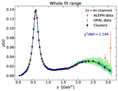
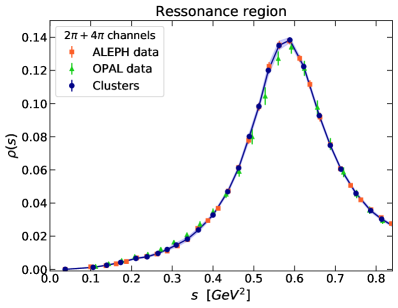
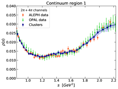
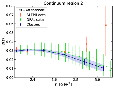
Figure 2: Result of the fit for the 68-cluster combination of the $2\pi+4\pi$ channels. The error bars represents non-inflated errors while inflated errors are represented by the blue band.

III.4 The inclusive $V$ non-strange spectral function.

The main decision to be made when combining the data into clusters is the choice of the clusters themselves. One possibility is the basis of the strategy used in Ref. [14]. In this strategy, small groups of data points consecutive in $s$ are assigned to clusters, after which each cluster is assigned an $s$ value according to Eq. (16). The algorithm described in Sec. III.2 is then applied. The choice of clusters can then be varied to find the combination which has both a $\chi^{2}/{\rm dof}$ close to unity and small errors on the sum-rule integrals $I^{(w)}_{\rm ex}(s_{0})$. A choice of too few data points per cluster could lead to an erratic point-to-point behavior that would not reflect any gain of information, while a choice of too many data points per cluster could lead to a loss of information. However, we should keep in mind that we are concerned with only two datasets for the $2\pi+4\pi$ contribution to the spectral function that will be combined, with one data set (ALEPH) being more precise than the other (OPAL). It is then reasonable to consider a combination largely based on the ALEPH energy bins, such that the majority of clusters contains at least one ALEPH data point. The cluster sizes near the $\rho$ peak will be narrower and widen with increasing $s$, since the ALEPH bin widths increase with $s$ in the region above the $\rho$ peak.

In order to construct the full covariance matrix $C$ to be used in the fit of Eq. (17) we first combine the covariances for the $2\pi$ and $4\pi$ $dB/ds$ distributions from ALEPH and OPAL, assuming at this stage no correlations between the two data sets. Then BF errors, as well as their correlations, are added into the full covariance matrix. This introduces correlations between ALEPH and OPAL. With the full covariance matrix and a choice of clusters in hand, the fit to Eq. (17) can be carried out.

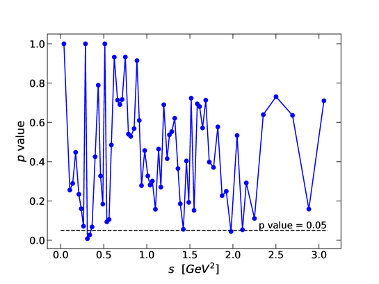
Figure 3: $p$-value distribution by cluster for the 68-cluster combination shown in Fig. 2.

Our final combination contains 68 clusters (a number not too far below the 79 bins of the 2013 ALEPH data set) and yields a $\chi^{2}$ per degree of freedom close to the unity:

$$\chi^{2}_{\rm min}/{\rm dof}=1.144\ ,$$ (22)

with a good $p$ value of $15\%$. The result of this fit, together with the ALEPH and OPAL data sets is shown in Fig. 2, where the error bars are the non-inflated errors obtained from Eq. (21), and the blue band represents the inflated errors obtained through local-$\chi^{2}$ inflation. The local $p$ value for each cluster is shown in Fig. 3. In the rest of this paper, we will choose to work with non-inflated errors. One expects fluctuations in $p$ value when combining these two data sets, and the local $p$ value is never unacceptably small. There is thus no reason to assume that values of the local $\chi^{2}/$dof signal discrepancies between the ALEPH and OPAL data. As we will see in Sec. IV, inflating the errors has no effect on $\alpha_{s}$.

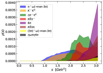
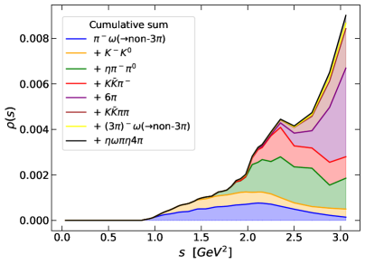
Figure 4: Residual modes contributions to the spectral function. Left panel: individual modes; right panel: cumulative residual-mode sums.

We explored different choices of the clusters, with the number of clusters $N_{\rm cl}$ ranging from 52 to 79 (the latter equaling the number of bins in the ALEPH data set). We found no significantly better fits with $N_{\rm cl}>68$. This is not surprising, because 68 is not much less than the total number of ALEPH data points, which form the more precise data set. In fact, we found equally good fits with $N_{\rm cl}<68$. However, we wish to have sufficiently many values of $I^{(w)}_{\rm exp}(s_{0})$ available to probe stability of the sum-rule fits to $I^{(w)}_{\rm exp}(s_{0})$ (cf.   Sec. IV), and thus do not want to choose $N_{\rm cl}$ too small.

With the combined $2\pi+4\pi$ spectral function in hand, the residual modes we need to add to obtain the inclusive spectral function, in order of decreasing BF size, are $\pi^{-}\omega(\to{\rm\mbox{non-}}3\pi)$, $K^{-}K^{0}$, $\eta\pi^{-}\pi^{0}$, $K\bar{K}\pi^{-}$, $6\pi$, $K\bar{K}2\pi$, $(3\pi)^{-}\omega(\to{\rm\mbox{non-}}3\pi)$ and $\eta\omega\pi\eta 4\pi$. In order to add these modes, a linear interpolation to the cluster $s^{(m)}$ values is performed individually for each mode. In the left panel of Fig. 4 the individual contribution to the spectral function for each residual mode is shown, while the right panel shows the cumulative effect, beginning with the $\pi^{-}\omega(\to{\rm\mbox{non-}}3\pi)$ contribution, then adding $K^{-}K^{0}$, then $\eta\pi^{-}\pi^{0}$, and so on. From these figures we also see that the residual modes $(3\pi)^{-}\omega(\to{\rm\mbox{non-}}3\pi)$ and $\eta\omega\pi\eta 4\pi$ with the smallest BFs already give negligible contributions to the inclusive spectral function total. This observation supports the conclusion already noted above that omitted contributions from yet-higher-multiplicity modes can be safely neglected in the region up to $s=m_{\tau}^{2}$ relevant to the current analysis.

Finally, the inclusive spectral function $\rho_{ud;V}(s)$ is given by the sum of the contributions from the combined $2\pi+4\pi$ and interpolated residual modes. Figure 5 shows the individual contributions as well as the sum. Notice that the residual modes give only a small contribution, which, moreover, is located toward the end of the $\tau$-decay spectrum. The final spectral function is displayed in Tab. 1 with inflated and non-inflated errors for the $2\pi+4\pi$ contribution.

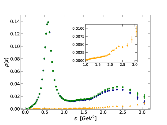
Figure 5: The non-strange $V$ combined spectral function. Total residual-mode contribution (yellow triangles), $2\pi+4\pi$ contribution (blue circles) and the total inclusive spectral function (green squares). The inset shows a blow up of the sum of residual-mode contributions above $s=1$ GeV².

$s$	$2\pi^{2}\rho_{ud;V}(s)$	$s$	$2\pi^{2}\rho_{ud;V}(s)$	$s$	$2\pi^{2}\rho_{ud;V}(s)$	$s$	$2\pi^{2}\rho_{ud;V}(s)$
0.038	0.000(00)(00)	0.106	0.024(04)(04)	0.139	0.049(06)(06)	0.174	0.082(07)(07)
0.211	0.131(09)(07)	0.238	0.150(10)(07)	0.265	0.190(16)(09)	0.288	0.236(11)(11)
0.310	0.290(26)(10)	0.337	0.360(24)(11)	0.364	0.470(25)(14)	0.400	0.647(16)(16)
0.436	0.926(20)(20)	0.463	1.208(24)(24)	0.489	1.583(42)(31)	0.512	1.942(37)(37)
0.536	2.372(63)(38)	0.562	2.668(52)(32)	0.588	2.733(32)(32)	0.622	2.417(33)(33)
0.661	1.832(29)(29)	0.688	1.478(22)(22)	0.714	1.195(21)(21)	0.751	0.905(19)(19)
0.787	0.700(17)(17)	0.814	0.599(16)(16)	0.853	0.484(14)(14)	0.886	0.413(12)(12)
0.912	0.382(10)(10)	0.939	0.343(11)(10)	0.976	0.310(10)(10)	1.012	0.272(10)(10)
1.038	0.273(10)(10)	1.065	0.267(10)(10)	1.100	0.257(12)(09)	1.137	0.254(09)(09)
1.164	0.243(10)(09)	1.197	0.251(10)(10)	1.237	0.248(09)(09)	1.263	0.259(09)(09)
1.290	0.266(10)(10)	1.325	0.276(10)(10)	1.362	0.284(10)(10)	1.389	0.279(13)(10)
1.425	0.299(18)(11)	1.460	0.291(10)(10)	1.488	0.292(13)(10)	1.515	0.305(11)(11)
1.549	0.298(15)(11)	1.586	0.319(11)(11)	1.614	0.319(11)(11)	1.648	0.313(11)(11)
1.685	0.335(12)(12)	1.726	0.355(13)(13)	1.775	0.394(13)(13)	1.825	0.413(15)(15)
1.874	0.461(17)(14)	1.923	0.488(18)(15)	1.978	0.541(31)(18)	2.049	0.589(20)(20)
2.111	0.618(46)(24)	2.156	0.640(23)(21)	2.251	0.664(30)(22)	2.353	0.696(25)(25)
2.501	0.681(29)(29)	2.692	0.594(44)(44)	2.882	0.474(79)(64)	3.057	0.383(78)(78)

Table 1: Total inclusive spectral function multiplied by $2\pi^{2}$. First errors are inflated errors, while second errors are not inflated. We recall that the parton-model value for $2\pi^{2}\rho_{ud;V}(s)$ is ${1\over 2}$.

Having obtained the combined inclusive spectral function, we can compare the moments $I^{(w)}_{\rm ex}(s_{0})$ which result to those obtained using the ALEPH and OPAL versions of $\rho_{ud;V}(s)$. We expect these to be consistent with one another, of course, but also expect the errors for the combined case to be the smallest. In Table 2 we compare values of the $I^{(w)}_{\rm ex}(s_{0})$ for $w=w_{0}$, $w_{2}$ and $w_{3}$ at $s_{0}=s_{0}^{*}\approx 1.5$ GeV² and $s_{0}=s_{0}^{**}\approx 2.9$ GeV². With the binning of the three data sets being somewhat different, the central values cannot be directly compared, because the spectral moments in the table have been computed at slightly different $s_{0}$ values on each line. However, the errors can be compared, as they vary only very slowly with $s_{0}$. The table thus indicates the gain in precision for spectral moments obtained from using the combined spectral function, instead of the ALEPH or OPAL spectral functions. It should also be borne in mind that the errors quoted for the ALEPH and OPAL entries in this table do not include additional, difficult-to-quantify systematic uncertainties associated with the use by ALEPH and OPAL of MC for the $s$-dependences of some of the residual exclusive-mode $\rho_{ud;V}(s)$ contributions. This additional systematic is absent from the evaluations of the spectral moments using our updated $\rho_{ud;V}(s)$ since the $s$-dependences of the numerically relevant contributions from all but the very small residual $K\overline{K}\pi\pi$ mode (where, instead, maximally conservative experimental constraints are used) are now based on direct experimental input.

	combined	ALEPH	OPAL
$I^{(w_{0})}_{\rm ex}(s_{0}^{*})$	0.03137(14)	0.03145(17)	0.03140(46)
$I^{(w_{0})}_{\rm ex}(s_{0}^{**})$	0.02952(29)	0.03133(65)	0.03030(170)
$I^{(w_{2})}_{\rm ex}(s_{0}^{*})$	0.02362(10)	0.02370(13)	0.02371(23)
$I^{(w_{2})}_{\rm ex}(s_{0}^{**})$	0.02016(8)	0.02081(14)	0.02038(27)
$I^{(w_{3})}_{\rm ex}(s_{0}^{*})$	0.01774(8)	0.01783(11)	0.01788(17)
$I^{(w_{3})}_{\rm ex}(s_{0}^{**})$	0.01574(6)	0.01614(8)	0.01580(14)

Table 2: Comparison of the spectral moments $I^{(w)}_{\rm ex}(s_{0})$ for $w=w_{0}$, $w=w_{2}$ and $w=w_{3}$ at two values of $s_{0}$, for the combined, the ALEPH, and the OPAL versions of the non-strange $V$ spectral function. We choose $s_{0}^{*}$ to be the closest value larger than or equal to $1.5$ GeV² for each case (combined, ALEPH, OPAL), and $s_{0}^{**}$ to be the closest value smaller than or equal to $2.9$ GeV² for each case. Note that, because the values of $s_{0}^{*}$ and $s_{0}^{**}$ are slightly different for the three cases, the central values cannot be directly compared. The errors can, however, be compared, as they vary slowly with $s_{0}$.

IV The strong coupling

In this section, we turn to the determination of $\alpha_{s}(m_{\tau})$ from the $V$ non-strange spectral function (and associated covariances) obtained in the previous section. We first briefly outline our strategy in Sec. IV.1, then present our results in Sec. IV.2. Further analysis and discussion of these results is contained in Sec. IV.3.

IV.1 Strategy

The $V$ spectral integrals $I^{(w)}_{\rm exp}(s_{0})$ for successive values of $s_{0}$ are highly correlated. Very strong correlations also exist between $I^{(w)}_{\rm exp}(s_{0})$ with different weights $w$. We find that it is possible to carry out standard $\chi^{2}$ fits taking into account all correlations when we limit ourselves to the weight $w_{0}$, while this is not the case when fits to combinations of two different weights over the same interval in $s_{0}$ are considered.

We will thus carry out two types of fits. First, since we need sensitivity to the DV parameters in Eq. (12) [12], we will always include the spectral integrals with the unpinched weight $w_{0}$ in our fits. Our most basic fit is a single-weight $\chi^{2}$ fit to $I^{(w_{0})}_{\rm exp}(s_{0})$ over an interval $s_{0}\in[s_{\rm min},s_{max}]$, where we will always choose $s_{max}$ equal to the largest of the cluster $s^{(m)}$ values. Since this is a non-linear fit, errors determined from the second-derivative matrix at $\chi^{2}_{\rm min}$ are not necessarily very meaningful, and we instead determine errors by varying each parameter such that $\chi^{2}=\chi^{2}_{\rm min}+1$. In all cases, we find that these errors are approximately symmetric, and so take the average of the negative and positive errors as our estimate for the error on each parameter. Because correlations are fully taken into account, we will also provide the $p$ value of these fits, and use this to determine optimal values of $s_{\rm min}$.

In the second class of fit, we carry out combined two-weight fits to $I^{(w_{0})}_{\rm exp}(s_{0})$ and one of the $I^{(w_{n})}_{\rm exp}(s_{0})$, with $n=2$, $3$ or $4$. These fits serve as consistency checks on the fits to $I^{(w_{0})}_{\rm exp}(s_{0})$ alone. For these fits, the combined two-weight correlation matrix is too singular to allow a fully correlated fit to be carried out. Thus, as in Refs. [9, 12, 13], we carry out “block-diagonal” fits, using a quadratic form in which all correlations between different $s_{0}$ values for each spectral integral are retained, but not those between spectral integrals with different weights. All correlations are fully included after the fit, when we obtain parameter error estimates for such block-diagonal fits by linear error propagation, as summarized in the appendix of Ref. [12]. To distinguish it from a true $\chi^{2}$ function, we will refer to the quadratic form minimized in this type of fit as the fit quality $Q^{2}$. The distinction is relevant since $Q^{2}$ is, in general, not a $\chi^{2}$-distributed quantity. While this makes it more difficult to characterize, in a quantitative manner, the quality of such a fit, the relative “goodness” of two such fits involving the same pair of weights, but different values of $s_{\rm min}$, can still be assessed by comparing the optimized results for their $Q^{2}$ values per degree of freedom. We emphasize again that the full data covariance matrix, including now also correlations between spectral moments with different weights, is taken into account in the error propagation.

A final complication is caused by the fact that the correlation matrices for $I^{(w_{3})}_{\rm exp}(s_{0})$ and $I^{(w_{4})}_{\rm exp}(s_{0})$ turn out to have very small eigenvalues, for the relevant values of $s_{\rm min}$, precluding even the block-diagonal fits with these moments if the full set of cluster values $s^{(m)}$ is used for the $s_{0}$ values in the fit. It turns out that this problem can be solved by “thinning” the data, as will be described in more detail in the following subsection. We emphasize again that these two-moment fits serve primarily as consistency checks on the fully correlated fits to $I^{(w_{0})}_{\rm exp}(s_{0})$.

IV.2 Results

We begin with fits to $I^{(w_{0})}_{\rm exp}(s_{0})$, using Eq. (3) with the right-hand side of this equation replaced by Eq. (11) with $w=w_{0}=1$. For the reasons explained in Sec. II.3 we will focus on FOPT, although we will briefly quote values obtained using CIPT as well.

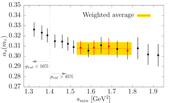
Figure 6: $\alpha_{s}(m_{\tau})$ of Table 3 as a function of $s_{\rm min}$. The yellow area correspond to the average reported in Eq. (23); this average is computed from the data points indicated in red (see text). The thin vertical dashed line separates the regions in which the $p$ values shown in Table 3 are smaller than 16% (to the left), from the region where they are larger than 45% (to the right).

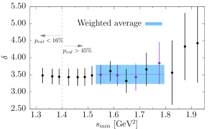
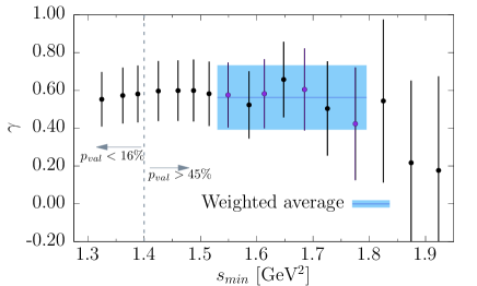
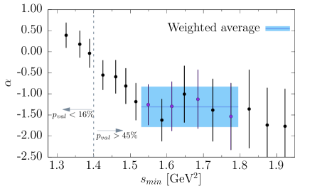
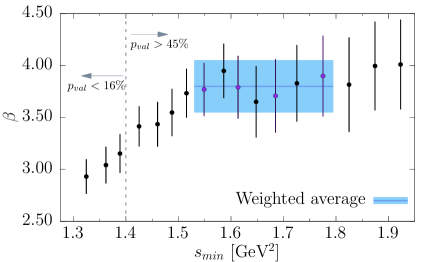
Figure 7: DV parameters of Table 3 as a function of $s_{\rm min}$. The blue areas correspond to the averages reported in Eq. (23); these averages are computed from the data points indicated in purple (see text). $\beta$ and $\gamma$ are in GeV^-2. The thin vertical dashed line separates the regions in which the $p$ values shown in Table 3 are smaller than 16% (to the left), from the region where they are larger than 45% (to the right).

$~{}~{}s_{\rm min}$	$\chi^{2}$/dof	$p$ value	$~{}~{}\alpha_{s}(m_{\tau})$	$~{}~{}~{}~{}\,\delta$	$\gamma$	$\alpha$	$\beta$
1.3246	30.71/22	0.10	0.3263(72)	3.48(22)	0.55(14)	$-$0.39(30)	2.93(17)
1.3619	28.56/21	0.12	0.3232(71)	3.46(23)	0.57(15)	$-$0.18(32)	3.04(18)
1.3886	26.63/20	0.15	0.3206(70)	3.45(23)	0.58(15)	$-$0.04(34)	3.15(19)
1.4251	17.96/19	0.53	0.3149(65)	3.43(25)	0.60(16)	$-$0.55(35)	3.41(19)
1.4602	17.91/18	0.46	0.3145(67)	3.43(25)	0.60(16)	$-$0.59(40)	3.43(22)
1.4877	16.43/17	0.49	0.3123(67)	3.44(26)	0.60(16)	$-$0.81(42)	3.55(23)
1.5154	12.69/16	0.70	0.3091(64)	3.48(28)	0.58(17)	$-$1.18(44)	3.73(24)
1.5490	12.57/15	0.64	0.3085(66)	3.50(28)	0.58(17)	$-$1.26(48)	3.77(26)
1.5863	9.97/14	0.76	0.3056(64)	3.61(30)	0.52(18)	$-$1.62(51)	3.95(26)
1.6136	7.65/13	0.87	0.3084(72)	3.49(31)	0.58(18)	$-$1.29(59)	3.79(30)
1.6479	6.52/12	0.89	0.3109(82)	3.32(35)	0.66(20)	$-$1.00(68)	3.65(35)
1.6849	6.27/11	0.85	0.3097(83)	3.43(40)	0.61(22)	$-$1.13(71)	3.71(36)
1.7256	5.71/10	0.84	0.3072(83)	3.66(49)	0.50(25)	$-$1.38(75)	3.83(37)
1.7752	5.51/9	0.79	0.3056(87)	3.84(62)	0.42(30)	$-$1.54(80)	3.90(39)
1.8249	5.33/8	0.72	0.308(11)	3.56(95)	0.54(44)	$-$1.36(96)	3.82(47)
1.8744	4.15/7	0.76	0.302(11)	4.3(1.0)	0.22(45)	$-$1.74(91)	4.00(44)
1.9230	4.13/6	0.66	0.301(12)	4.4(1.2)	0.18(52)	$-$1.77(92)	4.01(45)
1.9779	0.676/5	0.98	0.294(10)	5.4(1.1)	$-$0.19(45)	$-$1.58(85)	3.97(41)

Table 3: Results of fits to $I^{(w_{0})}_{\rm exp}(s_{0})$ employing the combined spectral function with 68 clusters, with $s_{\rm max}=3.0574$ GeV², $s_{\rm min}$ in GeV² and $\beta$ and $\gamma$ in GeV^-2.

The results ofour FOPT fits to $I^{(w_{0})}_{\rm exp}(s_{0})$ are shown in Table 3 for a range of $s_{\rm min}$ values lying between $1.3246$ and $1.9779$ GeV². The dependence of the fit results on $s_{\rm min}$ is also displayed in Fig. 6 for $\alpha_{s}(m_{\tau})$, and Fig. 7 for the DV parameters. Our first task is to determine the range of values of $s_{\rm min}$ from which to obtain our best estimate of $\alpha_{s}(m_{\tau})$. This selection is based on several observations. First, while all $p$ values are acceptable, those for $s_{\rm min}\in[1.4251,1.9779]$ GeV² are very good. Second, all fit parameters, including, in particular $\alpha$ and $\beta$, become stable for $s_{\rm min}\geq 1.5490$ GeV², while the fits become distinctly less accurate for $s_{\rm min}\geq 1.8249$ GeV², as the number of data points available to the fit becomes smaller. Finally, we observe that the $p$ value abruptly drops for $s_{\rm min}=1.3886$ GeV² and becomes systematically smaller if $s_{\rm min}$ is lowered below this value, signalling the expected breakdown of the theory description for low $s_{0}$. The results of our fits are based on the spectral function without error inflation in the combined 2$\pi$ +4$\pi$ channels. Inflating the errors only produces even higher $p$ values while leaving the fit parameters essentially unchanged. For example, for the fit with $s_{\rm min}=1.5863$ GeV² with error inflation we find a $p$ value of 88% and $\alpha_{s}(m_{\tau})=0.3053(66)$, to be compared with 76% and $\alpha_{s}(m_{\tau})=0.3056(64)$ given in Table 3.

Results for the parameters obtained from fits with nearby $s_{\rm min}$ are, of course, highly correlated. We will take the correlated average of the parameter values at $s_{\rm min}=1.5490$ GeV², $1.6136$ GeV², $1.6849$ GeV² and $1.7752$ GeV² as our best estimate for the value of each parameter, thinning out the seven points on the interval between $1.5490$ GeV² and $1.7752$ GeV² to lessen the impact of the very strong correlations between the parameter values at neighboring $s_{\rm min}$. With this strategy, we find the parameter values (statistical errors only)

$$\alpha_{s}(m_{\tau}) = 0.3077(65)\ ,\qquad(w_{0}\ ,\ \mbox{FOPT})$$ (23)

$$\delta = 3.51(28)\ ,$$

$$\gamma = 0.57(17)\ \mbox{GeV}^{-2}\ ,$$

$$\alpha = -1.31(48)\ ,$$

$$\beta = 3.81(26)\ \mbox{GeV}^{-2}\ .$$

The points used in obtaining these averages are those marked in red and purple in the shaded regions of Figs. 6 and 7, respectively.

We note that taking a straight average of the seven values inside the yellow window in Fig. 6 between $s_{\rm min}=1.5490$ and $1.7752$ GeV², and taking the smallest parameter error on this interval as the error on this average yields $\alpha_{s}(m_{\tau})=0.3080(64)$, a result almost identical to that in Eq. (23). We will take the result shown in Eq. (23) as our central value, with the slightly larger error shown there.

The fit to $I^{(w_{0})}_{\rm exp}(s_{0})$ for $s_{\rm min}=1.5490$ GeV² is displayed in the left panel of Fig. 8. The right panel of the same figure shows a comparison of the representation for $\rho_{ud;V}(s)$ obtained using the parameters of this fit with the combined experimental result obtained in Sec. III.

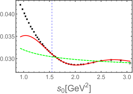
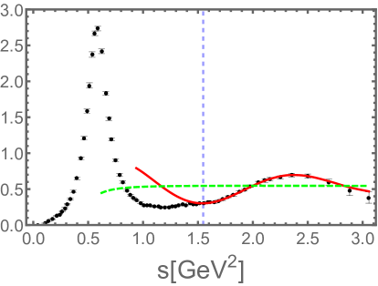
Figure 8: The spectral moment $I^{(w_{0})}_{\rm exp}(s_{0})$ from the fit with $s_{\rm min}=1.5490$ GeV² in Table 3 (left panel), and the resulting spectral function (right panel), multiplied by $2\pi^{2}$. The black symbols denote data points, the red solid curve the fit, and the green dashed curve the OPE part of the fit.

We have also carried out these fits using the CIPT prescription for the $D=0$ perturbative contributions, finding the values (again, statistical errors only)

$$\alpha_{s}(m_{\tau}) = 0.3239(87)\ ,\qquad(w_{0}\ ,\ \mbox{CIPT})$$ (24)

$$\delta = 3.35(28)\ ,$$

$$\gamma = 0.65(18)\ \mbox{GeV}^{-2}\ ,$$

$$\alpha = -1.33(49)\ ,$$

$$\beta = 3.80(26)\ \mbox{GeV}^{-2}\ .$$

We do not show figures equivalent to Figs. 6, 7 and 8, as they would look very similar. As is the case in all $\tau$-based $\alpha_{s}$ determinations, the CIPT value is about 5 percent larger than the FOPT value. The statistical error on the FOPT and CIPT values are about 2.1 and 2.6 percent, respectively. We note that the DV-parameter values are not significantly different between the FOPT and CIPT fits.

$~{}~{}s_{\rm min}$	$Q^{2}$/dof	$~{}~{}\alpha_{s}(m_{\tau})$	$~{}~{}~{}~{}\,\delta$	$\gamma$	$\alpha$	$\beta$	$10^{2}c_{6}$
1.5490	26.2/34	0.3085(67)	3.49(28)	0.58(17)	$-$1.44(52)	3.85(27)	$-$0.60(12)
1.5863	22.7/32	0.3073(69)	3.50(29)	0.58(18)	$-$1.57(58)	3.92(30)	$-$0.62(13)
1.6136	18.5/30	0.3101(80)	3.36(31)	0.65(18)	$-$1.24(68)	3.76(35)	$-$0.55(17)
1.6479	15.5/28	0.3117(89)	3.31(35)	0.67(20)	$-$1.08(78)	3.68(40)	$-$0.52(20)
1.6849	15.1/26	0.3106(90)	3.42(40)	0.62(21)	$-$1.20(81)	3.74(41)	$-$0.55(20)
1.7256	13.7/24	0.3082(90)	3.70(48)	0.49(24)	$-$1.44(85)	3.85(42)	$-$0.62(19)
1.7752	13.5/22	0.3076(97)	3.76(61)	0.46(29)	$-$1.50(91)	3.88(45)	$-$0.64(21)

Table 4: Results of block-diagonal fits to $I^{(w_{0})}_{\rm exp}(s_{0})$ and $I^{(w_{2})}_{\rm exp}(s_{0})$ employing the combined spectral function with 68 clusters, with $s_{\rm max}=3.0574$ GeV², $s_{\rm min}$ in GeV², $\beta$ and $\gamma$ in GeV^-2, $c_{6}$ in GeV⁶. Errors have been computed using linear error propagation.

In Table 4, we present the results for the block-diagonal simultaneous fits to $I^{(w_{0})}_{\rm exp}(s_{0})$ and $I^{(w_{2})}_{\rm exp}(s_{0})$, restricting our attention to the seven values of $s_{\rm min}$ used in obtaining the results in Eqs. (23) above. Taking a straight average of the seven values between $s_{\rm min}=1.5490$ GeV² and $1.7752$ GeV², and taking the smallest parameter error on this interval as the error on this average, we find the parameter values (statistical errors only)

$$\alpha_{s}(m_{\tau}) = 0.3091(69)\ ,\qquad(w_{0}\ \&\ w_{2}\ ,\ \mbox{FOPT})$$ (25)

$$\delta = 3.51(29)\ ,$$

$$\gamma = 0.58(18)\ \mbox{GeV}^{-2}\ ,$$

$$\alpha = -1.35(58)\ ,$$

$$\beta = 3.81(30)\ \mbox{GeV}^{-2}\ ,$$

$$c_{6} = -0.0059(13)\ \mbox{GeV}^{6}\ .$$

These parameter values are in excellent agreement with those in Eq. (23); of course, $c_{6}$ is new.

$~{}~{}s_{\rm min}$	$Q^{2}$/dof	$~{}~{}\alpha_{s}(m_{\tau})$	$~{}~{}~{}~{}\,\delta$	$\gamma$	$\alpha$	$\beta$	$10^{2}c_{6}$	$10^{2}c_{8}$
1.5490	3.23/7	0.3070(70)	3.37(34)	0.66(21)	$-$1.80(62)	4.05(33)	$-$0.71(12)	1.23(20)
1.5863	2.11/7	0.3068(74)	3.37(34)	0.66(21)	$-$1.88(73)	4.10(38)	$-$0.72(13)	1.25(22)
1.6136	2.19/5	0.3097(83)	3.38(35)	0.64(21)	$-$1.55(83)	3.92(43)	$-$0.66(15)	1.15(28)
1.6479	1.96/5	0.3076(82)	3.44(41)	0.63(23)	$-$1.72(83)	4.01(43)	$-$0.71(15)	1.24(27)
1.6849	1.33/5	0.3048(80)	3.62(46)	0.54(25)	$-$2.13(89)	4.22(45)	$-$0.78(14)	1.37(26)
1.7256	2.03/3	0.311(11)	3.41(70)	0.63(34)	$-$1.40(1.06)	3.85(53)	$-$0.65(23)	1.12(43)
1.7752	1.81/3	0.309(11)	3.4(1.0)	0.66(48)	$-$1.52(1.09)	3.91(54)	$-$0.68(25)	1.19(50)

Table 5: Results of block-diagonal fits to $I^{(w_{0})}_{\rm exp}(s_{0})$ and $I^{(w_{3})}_{\rm exp}(s_{0})$ employing the combined spectral function with 68 clusters, with $s_{\rm max}=3.0574$ GeV², $s_{\rm min}$ in GeV², $\beta$ and $\gamma$ in GeV^-2, $c_{6}$ in GeV⁶, $c_{8}$ in GeV⁸. Errors have been computed using linear error propagation. For each fit, every third value of $I^{(w_{0})}_{\rm exp}(s_{0})$ and $I^{(w_{3})}_{\rm exp}(s_{0})$ was used, starting from $s_{0}=s_{\rm min}$.

$~{}~{}s_{\rm min}$	$Q^{2}$/dof	$~{}~{}\alpha_{s}(m_{\tau})$	$~{}~{}~{}~{}\,\delta$	$\gamma$	$\alpha$	$\beta$	$10^{2}c_{6}$	$10^{2}c_{10}$
1.5490	2.89/7	0.3069(70)	3.37(34)	0.66(21)	$-$1.79(62)	4.04(33)	$-$0.69(12)	1.56(33)
1.5863	1.80/7	0.3065(74)	3.37(34)	0.66(21)	$-$1.87(73)	4.09(38)	$-$0.70(13)	1.60(38)
1.6136	1.90/5	0.3097(83)	3.38(35)	0.64(21)	$-$1.52(84)	3.91(44)	$-$0.64(16)	1.41(48)
1.6479	1.70/5	0.3076(82)	3.43(41)	0.63(23)	$-$1.69(83)	3.99(43)	$-$0.69(16)	1.57(48)
1.6849	1.10/5	0.3046(80)	3.61(46)	0.55(25)	$-$2.11(89)	4.21(45)	$-$0.76(15)	1.83(47)
1.7256	1.75/3	0.311(11)	3.39(70)	0.64(34)	$-$1.3(1.1)	3.82(53)	$-$0.62(24)	1.34(83)
1.7752	1.56/3	0.309(11)	3.3(1.0)	0.68(48)	$-$1.5(1.1)	3.89(55)	$-$0.65(27)	1.4(1.0)

Table 6: Results of block-diagonal fits to $I^{(w_{0})}_{\rm exp}(s_{0})$ and $I^{(w_{4})}_{\rm exp}(s_{0})$ employing the combined spectral function with 68 clusters, with $s_{\rm max}=3.0574$ GeV², $s_{\rm min}$ in GeV², $\beta$ and $\gamma$ in GeV^-2, $c_{6}$ in GeV⁶, $c_{10}$ in GeV¹⁰. For each fit, every third value of $I^{(w_{0})}_{\rm exp}(s_{0})$ and $I^{(w_{3})}_{\rm exp}(s_{0})$ was used, starting from $s_{0}=s_{\rm min}$.

In the case of simultaneous block-diagonal fits to $I^{(w_{0})}_{\rm exp}(s_{0})$ and $I^{(w_{n})}_{\rm exp}(s_{0})$ with $n=3,\ 4$, we find that the correlation matrices for the spectral moments with the doubly pinched weights $w_{3,4}$ have very small eigenvalues, leading to unstable fits with very large $Q^{2}$ values (equal to about 16 per degree of freedom for $s_{\rm min}\sim 1.6$ GeV²). The smallest eigenvalue in each such case is around $10^{-10}$, orders of magnitude smaller than the smallest eigenvalue for the set of $I^{(w_{2})}_{\rm exp}(s_{0})$ or $I^{(w_{0})}_{\rm exp}(s_{0})$ integrals, which are around $10^{-6}$ and $10^{-5}$, respectively. We find that if we “thin” the set of integrals used in the fit, starting at a given $s_{\rm min}$ and including only every second, third, etc., of the available higher $s_{0}$, the $Q^{2}/$dof drops rapidly to a value below $1$, and the fit stabilizes as we increase the degree of thinning. Tables 5 and 6 show the results of these fits for the cases $n=3$ and $n=4$, always thinning by a factor 3. Comparing the results of tables  3, 4, 5 and 6, we find good consistency among all these fits. Using the simplified averaging procedure employed above for $n=2$, we find the following parameter values (statistical errors only)

$$w_{0}\ \&\ w_{3}\qquad w_{0}\ \&\ w_{4}$$

$$\alpha_{s}(m_{\tau})\ \ = \ 0.3080(70)\qquad 0.3079(70)\quad(\mbox{FOPT})\ ,$$ (26)

$$\delta\ \ = \ \!\!\!\!\!\!3.43(34)\qquad 3.41(34)\ ,$$

$$\gamma\ \ = \ \!\!\!\!\!\!0.63(21)\qquad 0.64(21)\qquad[\mbox{GeV}^{-2}]\ ,$$

$$\alpha\ \ = \ \!\!\!\!\!\!\!\!\!\!\!-1.71(62)\qquad \!\!\!\!\!-1.68(62)\ ,$$

$$\beta\ \ = \ \!\!\!\!\!\!4.01(33)\qquad 3.99(33)\hskip 23.33147pt[\mbox{GeV}^{-2}]\ ,$$

$$c_{6}\ \ = \ \!\!\!\!\!\!\,-0.0070(12)\qquad \!\!\!\!\!-0.0068(12)\hskip 12.23447pt[\mbox{GeV}^{6}]\ ,$$

$$c_{8}\ \ = \!\!\!\!\!\!\!\!\!\!\!\,0.0122(20) \mbox{---}\hskip 53.49132pt[\mbox{GeV}^{8}]\ ,$$

$$c_{10}\ \ = 0.0153(33)\quad[\mbox{GeV}^{10}]\ .$$ —

where the first, respectively, second, column corresponds to a simultaneous fit to $I^{(w_{0})}_{\rm exp}(s_{0})$ and $I^{(w_{3})}_{\rm exp}(s_{0})$, respectively, $I^{(w_{0})}_{\rm exp}(s_{0})$ and $I^{(w_{4})}_{\rm exp}(s_{0})$. The results for those parameters also determined in the earlier fits also show good consistency with the values obtained in those earlier fits, reported in Eqs. (23) and (25). In addition, the values for the OPE coefficient $c_{6}$ shown in Tables 5 and 6 are consistent with those shown in Table 4. This constitutes an additional non-trivial consistency check.

We end this subsection with a comment. For reasons already explained, we did not construct the axial equivalent of the new inclusive spectral function $\rho_{ud;V}$ obtained in Sec. III, and thus did not carry out simultaneous fits to the $V$ and $A$ spectral functions. This precludes us from testing consistency between vector and axial channels, and from carrying out tests based on the Weinberg sum rules, as we did in Refs. [9, 12, 13]. Here we point out that such tests were always successful in the separate analyses of the ALEPH and OPAL non-strange inclusive spectral functions. We also note that our most precise results for $\alpha_{s}$ were always obtained from purely $V$ channel fits.

IV.3 Analysis

To finalize our result for $\alpha_{s}(m_{\tau})$, an estimate is required for the error resulting from the use of the four- or five-loop-truncated perturbation theory. This is obtained following the approach outlined at the end of Sec. II.3. We focus on the single-weight fit to $I^{(w_{0})}_{\rm exp}(s_{0})$ with $s_{\rm min}=1.5490$ GeV².

It turns out that among the various strategies for estimating this error discussed in Sec. II.3, varying $c_{51}$ by $\pm 50\%$ around thecentral value $c_{51}=283$ yields the largest, and thus most conservative, estimate of the truncation error. Symmetrizing the slightly asymmetric result produces an uncertainty of $\pm 0.0026$ on $\alpha_{s}(m_{\tau})$. Alternate error estimates based on removing order-$\alpha_{s}^{5}$ terms (i.e., setting $c_{5m}=0$), or removing both order-$\alpha_{s}^{4}$ and order-$\alpha_{s}^{5}$ terms (i.e., setting both $c_{4m}=0$ and $c_{5m}=0$) lead to differences equal to or smaller than the differences obtained from the $50\%$ variation in $c_{51}$ noted above.

These observations apply to the perturbative representation for $I^{(w_{0})}_{\rm th}(s_{0})$, and do not necessarily apply to spectral moments with other weights. Since moments with different weights have different perturbative behaviors [44, 45], we will take the difference between the values of $\alpha_{s}$ in Eqs. (23) and (25) to reflect an independent source of perturbative error. We multiply this difference by a factor two to take into account the fact that one of the two weights entering the fit leading to Eq. (25), $w_{0}$, was also used in obtaining the results quoted in Eqs. (23). This leads to an additional perturbative uncertainty of $\pm 0.0028$ on $\alpha_{s}$.

Combining the statistical error of Eq. (23) and the two perturbative uncertainties discussed above in quadrature, we obtain our final result for $\alpha_{s}$ at the $\tau$ mass scale:

$$\alpha_{s}(m_{\tau}) = 0.3077\pm 0.0065_{\rm stat}\pm 0.0038_{\rm pert}$$

$$= 0.3077\pm 0.0075\qquad\qquad(n_{f}=3\ ,\ \mbox{FOPT})\ ,$$

where the subscripts “stat” and “pert” refer to the statistical and the perturbative error, respectively.

As we explained in Sec. II, the $\tau$ scale is sufficiently low that non-perturbative effects are expected to be potentially non-negligible. For $I^{(w_{0})}_{\rm exp}(s_{0})$ non-perturbative contributions are generated by DVs, corresponding to the second term on the right-hand side of Eq. (11). It is interesting to quantify these effects. Even though the moment is dominated by perturbation theory, we find that the non-perturbative part of $I^{(w_{0})}_{\rm th}(s_{0})$, which is the moment most sensitive to non-perturbative effects, oscillates with an amplitude typically of order 20% of the $\alpha_{s}$-dependent part of the perturbative contribution (obtained by subtracting the $\alpha_{s}$-independent parton-model piece) with varying $s_{0}$.

The non-perturbative effect is thus small but significant, and this is not surprising. The non-perturbative part accounts for the oscillation seen in the spectral function in Fig. 8 (red curve), which cannot be accounted for by the OPE (green dashed curve). We believe that it is unlikely that any variation of the DV ansatz (12) that does an equally good job of fitting the data would lead to a variation in $\alpha_{s}$ larger than the error we obtained in Eq. (IV.3). It is clear that the data show the existence of non-zero DVs and, while a first-principles derivation from QCD does not exist, the main features of a DV ansatz cannot be taken to be arbitrary. As already pointed out in Sec. II, a minimal set of assumptions, based on commonly accepted properties of QCD such as, e.g., Regge behavior, leads to the parametrization (12) [25].

In fact, we have quantitative information on this issue, from the fits involving $I^{(w_{n})}_{\rm exp}(s_{0})$ with $n=2,3,4$, because of the single pinch in $w_{2}$, and the double pinch in $w_{3,4}$, which suppress DVs at different rates. Comparing the values of $\alpha_{s}(m_{\tau})$ in Eqs. (25) and (IV.2) to the value in Eq. (23), we see that the central value of $\alpha_{s}(m_{\tau})$ varies by no more than 0.0004, i.e., 0.13% of the central value, to be compared with the 2.3% relative error in Eq. (IV.3). Such variations are much smaller than we would expect were the larger DV contributions to the $w_{0}$ sum rule to have been incorrectly represented by the DV ansatz Eq. (12).

Running the result of Eq. (IV.3) to the $Z$-mass scale using the standard self-consistent combination of five-loop running [34, 35] with four-loop matching [79, 80] at the charm and bottom thresholds ($2m_{c}(m_{c})$ and $2m_{b}(m_{b})$, respectively, with $\overline{\rm MS}$ masses from the PDG [56]) we obtain the corresponding $n_{f}=5$ result

$$\alpha_{s}(m_{Z})=0.1171\pm 0.0010\qquad(n_{f}=5\ ,\ \mbox{FOPT})\ .$$ (28)

With five-loop running and four-loop matching the uncertainty due to the running is very small. If we perform the matching at $m_{c}(m_{c})$ and $m_{b}(m_{b})$ we find a shift of just 0.00009, which does not contribute to the final uncertainty.

To conclude this section, we compare our new value of $\alpha_{s}(m_{\tau})$ given in Eq. (IV.3) with those obtained from analyses of the ALEPH data [9], the OPAL data [13], and from $e^{+}e^{-}\to hadrons$ below $2$ GeV [81], where the latter was based on the combined electroproduction spectral data of Ref. [14]. These previously obtained values are

$$\alpha_{s}(m_{\tau}) = 0.325\pm 0.018\qquad(\mbox{OPAL\ data})\ ,$$ (29)

$$\alpha_{s}(m_{\tau}) = 0.296\pm 0.010\qquad(\mbox{ALEPH\ data})\ ,$$

$$\alpha_{s}(m_{\tau}) = 0.298\pm 0.017\qquad(e^{+}e^{-}\mbox{\ data})\ .$$

Previously, we quoted a weighted average of the two $\tau$-based values in Eq. (29), of the ALEPH-based and OPAL-based results, $\alpha_{s}(m_{\tau})=0.303\pm 0.009$, as our best determination from $\tau$ decays. This value and the values shown in Eq. (29) are in good agreement with our new, more precise value in Eq. (IV.3).

A direct comparison with other recent determinations of $\alpha_{s}$ from $\tau$ decays [5, 10] is problematic because they are all based on the truncated OPE strategy, which was shown in Refs. [26, 27] to be contaminated by uncontrolled systematic effects arising mainly from the neglect of unknown higher-order terms in the OPE in Refs. [5, 6, 7, 10]. The values of Refs. [5, 10] are also highly correlated, since they are based on the same general strategy and the same ALEPH data set. We note that the values of Refs. [5, 10] are significantly larger than ours $\alpha_{s}(m_{Z})=0.1199\pm 0.0015$, from Ref. [5] and $\alpha_{s}(m_{Z})=0.1197\pm 0.0015$, from Ref. [10].

V Conclusion

The determination of the strong coupling from hadronic $\tau$ decays has the potential to provide one of the most precise values among the many determinations from different methods that have appeared in the literature. It thus makes sense to aim for a determination from the combined experimental information available, and this is what we set out to do in this paper. This led us to construct a new non-strange vector, isovector spectral function, which is presented in Table 1 and Fig. 5.

In order to construct this spectral function, we combined the $\tau\to\pi^{-}\pi^{0}\nu_{\tau}$, $\tau\to 2\pi^{-}\pi^{+}\pi^{0}\nu_{\tau}$ and $\tau\to\pi^{-}3\pi^{0}\nu_{\tau}$ experimental data available from the ALEPH and OPAL collaborations, using the method employed before in Ref. [14]. The sum of these contributions constitutes 98% of the spectral function as measured by branching fraction.

Details of the contributions from the remaining exclusive channels, a number of which were estimated using Monte-Carlo, were not provided by ALEPH or OPAL. We have replaced the estimates for these residual-mode contributions using recent $\tau$ results for the $K^{-}K^{0}$ mode and the large amount of data now available, via CVC, from electroproduction experiments for the remaining residual modes, with conservative estimates of the systematic errors associated with this approach. As measured by the spectral moments shown in Table 2, this leads to a more accurate determination of the spectral function $\rho_{ud;V}(s)$, especially in the upper part of the $\tau$ kinematic range. This is a consequence of the fact that electroproduction data are not kinematically limited near the $\tau$ mass. We emphasize that the inclusive spectral function which results is a sum of $s$-dependent exclusive-mode contributions, all of which are now obtained from experiment and none of which require Monte-Carlo input any more.

One of the most important applications of this new combined data set is a determination of the strong coupling $\alpha_{s}$ at the $\tau$ mass scale. We employed previously developed methods using finite-energy sum rules to extract a new estimate of the $\overline{\rm MS}$ value of $\alpha_{s}(m_{\tau})$ from these data, which, when evolved to the $Z$ mass scale, produces a five-flavor result with an estimated precision of about 0.8%. Our final result is $\alpha_{s}(m_{Z})=0.1171\pm 0.0010$. We also revisited the question of how to best estimate the effect of truncating the perturbative expansion for the moments involved in these sum rules, arguing that, for a direct comparison with values obtained from other methods, the fixed-order resummation scheme is the appropriate one. Because the perturbative Adler function is known to a high order, $\alpha_{s}^{4}$, and the QCD $\beta$ function is known to an even higher order, $\alpha_{s}^{5}$, we arrived at a systematic error reflecting the use of perturbation theory which is quite small, 1.2% at the $\tau$ mass. We did not carry out an analysis of the perturbative error for CIPT, because of the issues discussed in Sec. II.3. For the same reasons, we emphasize that averaging the FOPT and CIPT values, or taking their difference as a measure of the perturbative error, would be misleading.

In order to carry out the analysis, we had to rely on the DV ansatz (12), and this introduces a model element into our framework. We note in this regard that, while no derivation of Eq. (12) from QCD exists, there are strong theoretical arguments supporting this ansatz based on commonly accepted conjectures about the spectrum of QCD [25], cf.   Sec. II.1. The consistency of the results of the fits presented above, which employ spectral moments with varying degrees of DV suppression, moreover, supports the consistency of our approach, as discussed in more detail in Sec. IV.3.

Our approach can be subjected to further tests when more precise $\tau$-decay data become available. With the strategy employed above, more precise data for just the low-multiplicity decay channels $\tau\to\pi^{-}\pi^{0}\nu_{\tau}$, $\tau\to 2\pi^{-}\pi^{+}\pi^{0}\nu_{\tau}$ and $\tau\to\pi^{-}3\pi^{0}\nu_{\tau}$ would produce further improvements to the inclusive non-strange vector isovector spectral function and allow for much higher precision tests of our framework. High-precision data for $\tau\to\pi^{-}\pi^{0}\nu_{\tau}$ are, in fact, already available [82], implying that similar data for the two four-pion channels would potentially have a significant impact on the determination of $\alpha_{s}$ from non-strange hadronic $\tau$ decays.

Finally, the new spectral function can also be used in other applications. It can be used to put constraints on low-energy constants in chiral perturbation theory, with next-to-next-to-leading-order theoretical representations being available [83, 84, 85]. Additional low-energy constants would become accessible were an updated non-strange axial vector spectral function to be obtained. Such an update is, however, more difficult, given the absence of any analogue of the electroproduction data used in improving many of the vector residual-mode contributions. We leave the consideration of the axial channel to future work.

Acknowledgments

We thank Alex Keshavarzi for discussions. We thank the ICTP South American Institute for Fundamental Research (SAIFR) at IFT-UNESP, where this work was initiated, for hospitality. DB is supported by the São Paulo Research Foundation (FAPESP) Grant No. 2015/20689-9 and by CNPq Grant No. 309847/2018-4. MG and WS are supported by the U.S. Department of Energy, Office of Science, Office of High Energy Physics, under Award No. DE-SC0013682. MVR is supported by FAPESP grant No. 2019/16957-9. KM is supported by a grant from the Natural Sciences and Engineering Research Council of Canada. SP is supported by CICYTFEDER-FPA2017-86989-P and by Grant No. 2017 SGR 1069. IFAE is partially funded by the CERCA program of the Generalitat de Catalunya.

References

- [1]
- [2] P. A. Baikov, K. G. Chetyrkin and J. H. Kühn, Order QCD Corrections to and Decays, Phys. Rev. Lett. 101, 012002 (2008) [arXiv:0801.1821 [hep-ph]].
- [3] R. Barate et al. [ALEPH Collaboration], Measurement of the spectral functions of axial-vector hadronic tau decays and determination of alpha(S)(M**2(tau)), Eur. Phys. J. C 4, 409 (1998).
- [4] S. Schael et al. [ALEPH Collaboration], Branching ratios and spectral functions of tau decays: Final ALEPH measurements and physics implications, Phys. Rept. 421, 191 (2005) [arXiv:hep-ex/0506072].
- [5] M. Davier, A. Hoecker, B. Malaescu, C. Z. Yuan and Z. Zhang, Update of the ALEPH non-strange spectral functions from hadronic decays, Eur. Phys. J. C 74, 2803 (2014) [arXiv:1312.1501 [hep-ex]].
- [6] K. Ackerstaff et al. [OPAL Collaboration], Measurement of the strong coupling constant alpha(s) and the vector and axial-vector spectral functions in hadronic tau decays, Eur. Phys. J. C 7, 571 (1999) [arXiv:hep-ex/9808019].
- [7] T. Coan et al. [CLEO], Measurement of from tau decays, Phys. Lett. B 356, 580 (1995).
- [8] S. Anderson et al. [CLEO], Hadronic structure in the decay , Phys. Rev. D 61, 112002 (2000) [arXiv:hep-ex/9910046 [hep-ex]].
- [9] D. Boito, M. Golterman, K. Maltman, J. Osborne and S. Peris, The strong coupling from the revised ALEPH data for hadronic decays, Phys. Rev. D 91, 034003 (2015) [arXiv:1410.3528 [hep-ph]].
- [10] A. Pich and A. Rodríguez-Sánchez, Determination of the QCD coupling from ALEPH decay data, Phys. Rev. D 94, 034027 (2016) [arXiv:1605.06830 [hep-ph]].
- [11] D. R. Boito, O. Catà, M. Golterman, M. Jamin, K. Maltman, J. Osborne and S. Peris, Duality violations in tau hadronic spectral moments, Nucl. Phys. B Proc. Suppl. 218, 104 (2011) [arXiv:1011.4426 [hep-ph]].
- [12] D. Boito, O. Catà, M. Golterman, M. Jamin, K. Maltman, J. Osborne and S. Peris, A new determination of from hadronic decays, Phys. Rev. D 84, 113006 (2011) [arXiv:1110.1127 [hep-ph]].
- [13] D. Boito, M. Golterman, M. Jamin, A. Mahdavi, K. Maltman, J. Osborne and S. Peris, An Updated determination of from decays, Phys. Rev. D 85, 093015 (2012) [arXiv:1203.3146 [hep-ph]].
- [14] A. Keshavarzi, D. Nomura and T. Teubner, Muon and : a new data-based analysis, Phys. Rev. D 97, 114025 (2018) [arXiv:1802.02995 [hep-ph]].
- [15] R. Shankar, Determination of the Quark-Gluon Coupling Constant, Phys. Rev. D 15, 755 (1977).
- [16] R. G. Moorhouse, M. R. Pennington and G. G. Ross, What Can Asymptotic Freedom Say About ?, Nucl. Phys. B 124, 285 (1977).
- [17] K. G. Chetyrkin and N. V. Krasnikov, Constraints on the Behavior of the Hadron Annihilation Cross-Section in Asymptotically Free Theories and in Theories with Anomalous Dimensions, Nucl. Phys. B 119, 174 (1977).
- [18] K. G. Chetyrkin, N. V. Krasnikov and A. N. Tavkhelidze, Finite Energy Sum Rules for the Cross-Section of Annihilation Into Hadrons in QCD, Phys. Lett. B 76, 83 (1978).
- [19] N. V. Krasnikov, A. A. Pivovarov and N. N. Tavkhelidze, The Use of Finite Energy Sum Rules for the Description of the Hadronic Properties of QCD, Z. Phys. C 19, 301 (1983).
- [20] E. G. Floratos, S. Narison and E. de Rafael, Spectral Function Sum Rules in Quantum Chromodynamics. 1. Charged Currents Sector, Nucl. Phys. B 155, 115 (1979).
- [21] R. A. Bertlmann, G. Launer and E. de Rafael, Gaussian Sum Rules in Quantum Chromodynamics and Local Duality, Nucl. Phys. B 250, 61 (1985).
- [22] E. Braaten, QCD Predictions for the Decay of the tau Lepton, Phys. Rev. Lett. 60, 1606 (1988).
- [23] E. Braaten, S. Narison, and A. Pich, QCD analysis of the hadronic width, Nucl. Phys. B 373, 581 (1992).
- [24] F. Le Diberder and A. Pich, Testing QCD with tau decays, Phys. Lett. B 289, 165 (1992).
- [25] D. Boito, I. Caprini, M. Golterman, K. Maltman and S. Peris, Hyperasymptotics and quark-hadron duality violations in QCD, Phys. Rev. D 97, 054007 (2018) [arXiv:1711.10316 [hep-ph]].
- [26] D. Boito, M. Golterman, K. Maltman and S. Peris, Strong coupling from hadronic decays: A critical appraisal, Phys. Rev. D 95, 034024 (2017) [arXiv:1611.03457 [hep-ph]].
- [27] D. Boito, M. Golterman, K. Maltman and S. Peris, Evidence against naive truncations of the OPE from hadrons below charm, Phys. Rev. D 100, 074009 (2019) [arXiv:1907.03360 [hep-ph]].
- [28] D. Boito, M. Golterman, K. Maltman and S. Peris, Determining from hadronic decay: the pitfalls of truncating the OPE, SciPost Phys. Proc. 1, 053 (2019) [arXiv:1811.01581 [hep-ph]].
- [29] A. A. Pivovarov, Renormalization group analysis of the tau-lepton decay within QCD, Z. Phys. C 53, 461 (1992) [Sov. J. Nucl. Phys. 54, 676 (1991)] [Yad. Fiz. 54, 1114 (1991)] [arXiv:hep-ph/0302003].
- [30] F. Le Diberder and A. Pich, The perturbative QCD prediction to R(tau) revisited, Phys. Lett. B 286, 147 (1992).
- [31] Y.-S. Tsai, Decay Correlations of Heavy Leptons in Lepton+ Lepton-, Phys. Rev. D 4, 2821 (1971) [Erratum, ibid. D 13, 771 (1976)].
- [32] M. Jamin, Contour-improved versus fixed-order perturbation theory in hadronic tau decays, JHEP 0509, 058 (2005) [hep-ph/0509001].
- [33] M. Beneke and M. Jamin, and the hadronic width: fixed-order, contour-improved and higher-order perturbation theory, JHEP 0809, 044 (2008) [arXiv:0806.3156 [hep-ph]].
- [34] P. A. Baikov, K. G. Chetyrkin and J. H. Kühn, Five-Loop Running of the QCD coupling constant, Phys. Rev. Lett. 118, 082002 (2017) [arXiv:1606.08659 [hep-ph]].
- [35] F. Herzog, B. Ruijl, T. Ueda, J. A. M. Vermaseren and A. Vogt, The five-loop beta function of Yang-Mills theory with fermions, JHEP 1702, 090 (2017) [arXiv:1701.01404 [hep-ph]].
- [36] E. C. Poggio, H. R. Quinn, S. Weinberg, Smearing the Quark Model, Phys. Rev. D 13, 1958 (1976).
- [37] O. Catà, M. Golterman, S. Peris, Possible duality violations in tau decay and their impact on the determination of alpha(s), Phys. Rev. D 79, 053002 (2009) [arXiv:0812.2285 [hep-ph]].
- [38] B. Blok, M. A. Shifman and D. X. Zhang, An illustrative example of how quark-hadron duality might work, Phys. Rev. D 57, 2691 (1998) [Erratum, ibid. D 59, 019901 (1999)] [arXiv:hep-ph/9709333].
- [39] I. I. Y. Bigi, M. A. Shifman, N. Uraltsev and A. I. Vainshtein, Heavy flavor decays, OPE and duality in two-dimensional ’t Hooft model, Phys. Rev. D 59, 054011 (1999) [hep-ph/9805241].
- [40] M. A. Shifman, Quark hadron duality, [hep-ph/0009131].
- [41] M. Golterman, S. Peris, B. Phily and E. de Rafael, Testing an approximation to large N(c) QCD with a toy model, JHEP 0201, 024 (2002) [hep-ph/0112042].
- [42] O. Catà, M. Golterman, S. Peris, Duality violations and spectral sum rules, JHEP 0508, 076 (2005) [hep-ph/0506004].
- [43] O. Catà, M. Golterman, S. Peris, Unraveling duality violations in hadronic tau decays, Phys. Rev. D 77, 093006 (2008) [arXiv:0803.0246 [hep-ph]].
- [44] M. Beneke, D. Boito and M. Jamin, Perturbative expansion of tau hadronic spectral function moments and extractions, JHEP 1301, 125 (2013) [arXiv:1210.8038 [hep-ph]].
- [45] D. Boito and F. Oliani, Renormalons in integrated spectral function moments and extractions, Phys. Rev. D 101, 074003 (2020) [arXiv:2002.12419 [hep-ph]].
- [46] K. Maltman, Constraints on hadronic spectral functions from continuous families of finite energy sum rules, Phys. Lett. B 440, 367 (1998) [hep-ph/9901239].
- [47] C. A. Dominguez and K. Schilcher, Chiral sum rules and duality in QCD, Phys. Lett. B 448, 93 (1999) [hep-ph/9811261].
- [48] M. Beneke, Renormalons, Phys. Rept. 317, 1 (1999) [hep-ph/9807443].
- [49] A. H. Hoang and C. Regner, Borel Representation of Hadronic Spectral Function Moments in Contour-Improved Perturbation Theory, arXiv:2008.00578 [hep-ph].
- [50] D. Boito, P. Masjuan and F. Oliani, Higher-order QCD corrections to hadronic decays from Padé approximants, JHEP 08, 075 (2018) [arXiv:1807.01567 [hep-ph]].
- [51] I. Caprini, Higher-order perturbative coefficients in QCD from series acceleration by conformal mappings, Phys. Rev. D 100, 056019 (2019) [arXiv:1908.06632 [hep-ph]].
- [52] M. Davier, S. Descotes-Genon, A. Höcker, B. Malaescu and Z. Zhang, The determination of from decays revisited, Eur. Phys. J. C 56, 305 (2008) [arXiv:0803.0979 [hep-ph]].
- [53] J. P. Lees et al. [BaBar Collaboration], Measurement of the spectra function for the decay, Phys. Rev. D 98, 032010 (2018) [arXiv:1806.10280 [hep-ex]].
- [54] B. Aubert, et al. [BaBar Collaboration], Measurements of , and cross sections using initial state radiation events, Phys. Rev. D 77, 092002 (2008) [arXiv:0710.4451 [hep-ex]].
- [55] Y. Amhis, et al. [HFLAV Collaboration], Averages of -hadron, -hadron and -lepton properties as of 2018, arXiv:1909.12524 [hep-ex].
- [56] P. A. Zyla, et al. [Particle Data Group], Prog. Theor. Exp. Phys. 2020, 083C01 (2020).
- [57] J. Erler, Electroweak radiative corrections to semileptonic tau decays, Rev. Mex. Fis. 50, 200 (2004) [hep-ph/0211345].
- [58] G. D’Agostini, On the use of the covariance matrix to fit correlated data, Nucl. Instrum. Meth. A 346, 306 (1994).
- [59] R. D. Ball et al. [NNPDF], Fitting Parton Distribution Data with Multiplicative Normalization Uncertainties, JHEP 05, 075 (2010) [arXiv:0912.2276 [hep-ph]].
- [60] J. P. Lees et al. [BaBar Collaboration], Measurement of the cross section using initial-state radiation at BABAR, Phys. Rev. D96, 092009 (2017) [arXiv:1709.01171 [hep-ex]].
- [61] M. Achasov et al. [SND Collaboration], Updated measurement of the cross section with the SND detector, Phys. Rev. D 94, 112001 (2016) [arXiv:1610.00235 [hep-ex]].
- [62] V. M. Aulchenko, et al. [SND Collaboration], Measurement of the cross section in the center-of-mass energy range 1.22-2.00 GeV with the SND detector at the VEPP-2000 collider, Phys. Rev. D 91, 052013 (2015) [arXiv:1412.1971 [hep-ex]].
- [63] M. N. Achasov, et al. [SND Collaboration], Measurement of the cross section with the SND detector at the VEPP-2000 collider, Phys. Rev. D 97, 012008 (2018) [arXiv:1711.08862 [hep-ex]].
- [64] J. P. Lees, et al. [BaBar Collaboration], Study of the process using initial state radiation, Phys. Rev. D 97, 052007 (2018) [arXiv:1801.02960 [hep-ex]].
- [65] J. P. Lees, et al. [BaBar Collaboration] Study of the reactions and at center-of-mass energies from threshold to 4.35 GeV using initial-state radiation, Phys. Rev. D 98, 112015 [arXiv:1810.11962 [hep-ex]].
- [66] S. S. Gribanov, et al., Measurement of the cross section with the CMD-3 detector at the VEPP-2000 collider, JHEP 01, 112 (2020) [arXiv:1907.08002 [hep-ex]].
- [67] We thank Sergei Gribanov for providing the inverse error matrix for the results of Ref. [66].
- [68] K. Inami, et al. [Belle Collaboration], Precise measurement of hadronic tau-decays with an eta meson, Phys. Lett. B 672, 209 (2009) [arXiv:0811.0088 [hep-ex]].
- [69] B. Aubert, et al. [BaBar Collaboration], The , and cross sections at center-of-mass energies from production threshold to 4.5 GeV measured with initial-state radiation, Phys. Rev. D 73, 052003 (2006) [arXiv:hep-ex/0602006].
- [70] P. A. Lukin, et al. [CMD-3 Collaboration], Study of the process in the C.M. energy range 1.5-2.0 GeV with the CMD-3 detector, Phys. Lett. B 723, 82 (2013) [arXiv:1302.0053 [hep-ex]].
- [71] M. N. Achasov, et al. [SND Collaboration], Recent results from SND detector at VEPP-2000 collider, EPJ Web Conf. 212, 04002 (2019)
- [72] R. R. Akhmetshin, et al. [CMD-3 Collaboration], Study of the process in the c.m. energy range 1394-2005 MeV with the CMD-3 detector, Phys. Lett. B 773, 2015 (2017) [arXiv:1706.06267 [hep-ex]].
- [73] M. N. Achasov, et al. [SND Collaboration], Measurement of the cross section below 2 GeV, Phys. Rev. D 99, 112004 (2019) [arXiv:1903.09307 [hep-ex]].
- [74] Thanks to Alex Keshavarzi for providing us with the results of the full six-mode cross section sum which result from the analysis of then-existing experimental cross sections reported in Ref. [14].
- [75] We thank Eugeny Solodov for providing tables of these cross sections, which are shown in Figures 18 and 19 of Ref. [69], but not explicitly tabulated there.
- [76] J. P. Lees, et al. [BaBar Collaboration], Study of the reactions and at center-of-mass energies from threshold to 4.35 GeV using initial-state radiation, Phys. Rev. D 98, 112015 (2018) [arXiv:1810.11962 [hep-ex]].
- [77] B. Aubert, et al. [BaBar Collaboration], The , , and cross sections measured with initial-state radiation, Phys. Rev. D 76, 092005 (2007) (Erratum ibid. 77, 119902 (2008)) [arXiv:0708.2461 [hep-ex]].
- [78] M. N. Achasov, et al. [SND Collaboration], Study of the process in the energy range GeV with the SND detector, Phys. Rev. D 94, 032010 (2016) [arXiv:1606.06481 [hep-ex]].
- [79] Y. Schröder and M. Steinhauser, Four-loop decoupling relations for the strong coupling, JHEP 01, 051 (2006) [arXiv:hep-ph/0512058 [hep-ph]].
- [80] K. G. Chetyrkin, J. H. Kühn and C. Sturm, QCD decoupling at four loops, Nucl. Phys. B 744, 121 (2006) [arXiv:hep-ph/0512060 [hep-ph]].
- [81] D. Boito, M. Golterman, A. Keshavarzi, K. Maltman, D. Nomura, S. Peris and T. Teubner, Strong coupling from hadrons below charm, Phys. Rev. D 98 074030 (2018) [arXiv:1805.08176 [hep-ph]].
- [82] M. Fujikawa et al. [Belle], High-Statistics Study of the Decay, Phys. Rev. D 78, 072006 (2008) [arXiv:0805.3773 [hep-ex]].
- [83] E. Golowich and J. Kambor, Inverse moment chiral sum rules, Phys. Rev. D 53, 2651 (1996) [arXiv:hep-ph/9509304 [hep-ph]].
- [84] E. Golowich and J. Kambor, Chiral sum rules to second order in quark mass, Phys. Rev. Lett. 79, 4092 (1997) [arXiv:hep-ph/9707341 [hep-ph]].
- [85] G. Amoros, J. Bijnens and P. Talavera, Two point functions at two loops in three flavor chiral perturbation theory, Nucl. Phys. B 568, 319 (2000) [arXiv:hep-ph/9907264 [hep-ph]].